FIAN/TD-07/04

ITEP/TH-33/04

Non-Abelian Vortices in N=1* Gauge Theory

V. Markov^a,d , A. Marshakov^b,c and A. Yung^a,c

^aPetersburg Nuclear Physics Institute, Gatchina, Russia

^bTheory Department, Lebedev Physics Institute, Moscow, Russia

^cInstitute of Theoretical and Experimental Physics, Moscow, Russia

^dHelmholtz Institut für Strahen und Kernphysik, Bonn University, Germany

Abstract

We consider the ${\cal N}=1^{*}$ supersymmetric $SU(2)$ gauge theory and demonstrate that the $Z_{2}$ vortices in this theory acquire orientational zero modes, associated with the rotation of magnetic flux inside $SU(2)$ group, and turn into the non-Abelian strings, when the masses of all chiral fields become equal. These non-Abelian strings are not BPS-saturated. We study the effective theory on the string world sheet and show that it is given by two-dimensional non-supersymmetric $O(3)$ sigma model. The confined ’t Hooft-Polyakov monopole is seen as a junction of the $Z_{2}$-string and anti-string, and as a kink in the effective world sheet sigma model. We calculate its mass and show that besides the four-dimensional confinement of monopoles, they are also confined in the two-dimensional theory: the monopoles stick to anti-monopoles to form the meson-like configurations on the strings they are attached to.

1 Introduction

The idea of confinement as a dual Meissner effect upon condensation of monopoles was suggested many years ago by ’t Hooft, Mandelstam and Polyakov [1]. Understanding of the electomagnetic duality in ${\cal N}=2\;$supersymmetric gauge theories allowed Seiberg and Witten to present the quantitative description of this phenomenon [2, 3].

Recall, first, the basic idea of the confinement mechanism [1]. Once magnetic (electric) charges condense, the electric (magnetic) flux is confined in the Abrikosov-Nielsen-Olesen (ANO) flux tube [4] connecting heavy trial electric (magnetic) charge and anti-charge. The energy of the ANO string increases lineary with its length. This ensures the linear increasing confining potential between the heavy electric (magnetic) charges and anti-charges.

Later studies of confinement in ${\cal N}=2\;$QCD showed [5, 6, 7, 8, 9] that generally confinement in this theory is essentially Abelian. At the first stage, the gauge group is broken down to an Abelian subgroup at larger scale by VEV’s of the adjoint scalars. Then the Abelian subgroup is broken down completely (or to its discrete subgroup) at much smaller energy scale by condensation of the quarks or monopoles. At the second stage the Abelian ANO flux tubes are formed leading to the confinement of magnetic or electric charges respectively.

However if one thinks of understanding the confinement mechanism in real QCD or in ${\cal N}=1\;$gauge theories, a somewhat different pattern of the gauge symmetry breaking without this ”Abelization” is probably needed [10]. In particular, the flux tubes should have some non-Abelian features, which were recently found in [11] in the context of ${\cal N}=2\;$QCD with the gauge group $SU(2)\times U(1)$ with two flavors of quarks, perturbed by the Fayet-Iliopoulos (FI) term [12] of the $U(1)$ factor, (more generally $SU(N)\times U(1)$ gauge group with $N$ flavors of quarks, see also [13]; similar results in three dimensions were obtained in [14]). At large values of the quark masses the vacuum where both flavors of squarks condense is in the weak coupling regime, and quasiclassical analysis is applicable. Flux tubes in this vacuum were found in [10], and it was demonstrated in [11] that in the limit of equal quark masses the diagonal $SU(2)$ subgroup of global gauge and flavor groups (called $SU(2)_{C+F}$) remains unbroken both by condensates of adjoint and fundamental scalars. It turns out, that existence of this unbroken subgroup ensures, that elementary BPS flux tubes acquire the orientational modes, associated with the rotation of the color magnetic flux, and these modes make the strings to be non-Abelian

Let us note that the flux tubes in non-Abelian theories at weak coupling were studied in numerous papers in recent years [16, 17, 18, 19, 20, 21]. In particular, the $Z_{N}$ strings associated with the center of gauge group were constructed. However, in all these constructions the flux was always directed along a fixed vector (in the Cartan subalgebra), and no moduli which could govern its orientation in the group space were ever found.

In this paper we suggest the simpler model for non-Abelian strings (compare to [11, 14]). We consider the ${\cal N}=1$^∗ supersymmetric $SU(2)$ gauge theory, or the ${\cal N}=4\;$theory with the mass terms for three ${\cal N}=1$ chiral superfields, and we take two equal masses, say $m_{1}=m_{2}=m$, while the third mass $m_{3}$ is generically distinct. The ${\cal N}=4\;$supersymmetry is the broken down to ${\cal N}=1$, unless $m_{3}=0$ when the theory has ${\cal N}=2\;$supersymmetry and becomes ${\cal N}=2\;$gauge theory with adjoint matter (more strictly two flavors of adjoint matter with equal masses).

Classically the vacuum structure of this theory was studied in [22], while the quantum effects were taken into account in [23], using the parallels between the Seiberg-Witten theories and integrable systems [24], of which the deformed ${\cal N}=4\;$theory together with the integrable Calogero-Moser family is the most elegant example (see also [25]). The ${\cal N}=4\;$theory with $SU(2)$ gauge group has three vacua, for small coupling $g\ll 1$ one of these vacua is in the weak coupling. All three adjoint scalars condense in this vacuum, therefore it is called Higgs vacuum [22, 23]. Other two vacua of the theory are always in the strong coupling, for small $m_{3}$ these are the monopole and dyon vacua of the perturbed ${\cal N}=2\;$theory [2].

In this paper we concentrate on the Higgs vacuum in the weak coupling regime. In this vacuum the gauge group $SU(2)$ is broken down to $Z_{2}$ by the adjoint scalar VEV’s, therefore there are stable $Z_{2}$ non-BPS flux tubes associated with the $\pi_{1}(SU(2)/Z_{2})=Z_{2}$. Note, that as soon as electric (color) charges develop VEV’s, the $Z_{2}$ strings carry magnetic fluxes and give rise to the confinement of monopoles. In the $SU(2)$ theory there is a ’t Hooft-Polyakov monopole [26] with a unit magnetic charge. Since the $Z_{2}$-string’s charge is $1/2$, it cannot end on a monopole (and this is the reason for the stability of $Z_{2}$ strings). Instead, the confined monopole appears to be a junction of the $Z_{2}$-string and anti-string (monopoles as string junctions were considered earlier in [27, 28, 29] and recently as junctions of the non-Abelian BPS strings in [13, 30]). Note that it was shown in [31, 32, 10, 33, 34] that in different models the monopole fluxes match those of the flux tubes, hence the monopoles can be confined by one or several strings.

We show that at the special value $m_{3}=m$ there is a diagonal $O(3)_{C+F}$ subgroup of the global gauge group $SU(2)$ and flavor $O(3)$ group, unbroken by vacuum condensates. Like in [11, 14], the presence of this group leads to emergence of orientational zero modes of the $Z_{2}$-strings associated with rotation of the color magnetic flux of a string inside the $SU(2)$ gauge group, which makes a $Z_{2}$ string genuinely non-Abelian.

Next, we derive the two-dimensional effective theory for the orientational zero modes on the string world sheet. It turn out to be (a non-supersymmetric!) two-dimensional $O(3)$ sigma model . Note, that effective world sheet theory for the BPS non-Abelian strings, considered in [14, 11, 29, 13, 30], is the ${\cal N}=2\;$SUSY $O(3)$ sigma model (or the ${\cal N}=2\;$SUSY $CP^{N-1}$ model for the gauge group $SU(N)\times U(1)$). Here we deal with the non-BPS strings therefore the effective world sheet theory is not supersymmetric (to be called just $O(3)$ sigma model in what follows). We also consider the case when $m_{3}$ is not exactly equal to $m$, with $\Delta m\equiv|m_{3}-m|\ll m$. In this case a shallow potential in the sigma model is generated, which makes it classically massive.

Then we discuss the confined monopole or a junction of non-Abelian $Z_{2}$-strings. We identify this monopole as an $O(3)$ sigma model kink [29, 13, 30] and calculate its mass. Classically the mass of this monopole vanishes in the limit $\Delta m\to 0$, while its size become infinite (cf. with [39]). We show, however, that this does not happen in quantum theory. When the non-perturbative effects in the $O(3)$ sigma model are taken into account, the monopole mass is determined by the dynamical scale of the $O(3)$ sigma model $\Lambda_{\sigma}$, and its size remains finite (of order of $\Lambda_{\sigma}^{-1}$).

Finally, we demonstrate that besides the four-dimensional confinement, which ensures that the monopoles are attached to the strings, they are also confined in the two-dimensional sense. Namely, the monopoles stick to the anti-monopoles on the string they are attached to, and form a meson-like configuration.

The paper is organized as follows. In Sect. 2 we review the ${\cal N}=1$^∗ gauge theory near the Higgs vacuum. In Sect. 3 we construct solutions for the Abelian $Z_{2}$-strings. First, we consider the Abelian limit of small $m_{3}$, when the theory has ${\cal N}=2\;$supersymmetry and possesses the whole tower of ANO Abelian BPS strings. When we increase $m_{3}$, all strings with multiple winding numbers become unstable, and we are left with lightest stable $Z_{2}$-strings. In Sect. 4 we take the limit $m_{3}=m$ and construct the orientational zero modes of the non-Abelian $Z_{2}$-strings. In Sect. 5 we derive the effective world sheet theory for these strings and in Sect. 6 consider its dynamics. Sect. 7 contains our conclusions.

2 The model

In terms of ${\cal N}=1\;$supermultiplets, the ${\cal N}=4\;$supersymmetric gauge theory with the $SU(2)$ gauge group contains a vector multiplet, consisting of the gauge field $A_{\mu}^{a}$ and gaugino $\lambda^{\alpha a}$, and three chiral multiplets $\Phi^{a}_{A}$, $A=1,2,3$, all in the adjoint representation of the gauge group, with $a=1,2,3$ being the $SU(2)$ color index. The superpotential of the ${\cal N}=4\;$gauge theory reads

$$\begin{array}[]{c}W_{{\cal N}=4}=-\frac{\sqrt{2}}{g^{2}}\varepsilon_{abc}\Phi_{1}^{a}\Phi_{2}^{b}\Phi_{3}^{c}.\end{array}$$ (2.1)

One can deform this theory, breaking ${\cal N}=4\;$supersymmetry down to ${\cal N}=2$, by adding the mass terms with equal masses $m$, say for the first two flavors of the adjoint matter

$$\begin{array}[]{c}W_{{\cal N}=2}={m\over 2g^{2}}\sum_{A=1,2}\left(\Phi_{A}^{a}\right)^{2}\end{array}$$ (2.2)

Then the third flavor combines with the vector multiplet to form a ${\cal N}=2\;$vector supermultiplet, while the first two flavors (2.2) can be treated as ${\cal N}=2$ massive adjoint matter. One can further break supersymmetry down to ${\cal N}=1$, adding a mass term to the $\Phi_{3}$ multiplet

$$\begin{array}[]{c}W_{{\cal N}=1^{*}}={m_{3}\over 2g^{2}}\left(\Phi_{3}^{a}\right)^{2}\end{array}$$ (2.3)

Then bosonic part of the action reads

$$\begin{array}[]{c}S_{{\cal N}=1^{*}}={1\over g^{2}}\int d^{4}x\left(\frac{1}{4}\left(F_{\mu\nu}^{a}\right)^{2}+\sum_{A}\left|D^{\rm adj}_{\mu}\ \Phi_{A}^{a}\right|^{2}+\frac{1}{2}\sum_{A,B}\left[(\bar{\Phi}_{A}\bar{\Phi}_{B})(\Phi_{A}\Phi_{B})-(\bar{\Phi}_{A}\Phi_{B})(\bar{\Phi}_{B}\Phi_{A})\right]+\right.\\ \left.+\sum_{A}\left|\frac{1}{\sqrt{2}}\varepsilon_{abc}\varepsilon^{ABC}\Phi^{b}_{B}\Phi^{c}_{C}-m_{A}\Phi^{a}_{A}\right|^{2}\right)+\ {\rm fermionic\ \ terms},\end{array}$$ (2.4)

where $F_{\mu\nu}^{a}=\partial_{\mu}A_{\nu}^{a}-\partial_{\nu}A_{\mu}^{a}+\varepsilon^{abc}A_{\mu}^{b}A_{\nu}^{c}$, $D^{\rm adj}_{\mu}\ \Phi_{A}^{a}=\partial_{\mu}\Phi^{a}_{A}+\varepsilon^{abc}A_{\mu}^{b}\Phi^{c}_{A}$, and we use the same notations $\Phi^{a}_{A}$ for the scalar components of the corresponding chiral superfields.

In this paper we are going to study the so called Higgs vacuum of the theory (2.4), when all three adjoint scalars develop the VEV’s of the order of $m,\sqrt{mm_{3}}$. The scalar condensates $\Phi^{a}_{A}$ can be written in the form of the following 3$\times$3 color-flavor matrix (convenient for the $SU(2)$ gauge group and three ${\cal N}=4\;$”flavors”)

$$\begin{array}[]{c}\langle\Phi_{A}^{a}\rangle=\frac{1}{\sqrt{2}}\left(\begin{array}[]{ccc}\sqrt{mm_{3}}&0&0\\ 0&\sqrt{mm_{3}}&0\\ 0&0&m\end{array}\right),\end{array}$$ (2.5)

and these VEV’s break completely the $SU(2)$ gauge group. The masses of the W-bosons $A_{\mu}^{1,2}$ are

$$\begin{array}[]{c}m^{2}_{1,2}=m^{2}+mm_{3},\end{array}$$ (2.6)

while the mass of the ”photon” $A_{\mu}^{3}$ is

$$\begin{array}[]{c}m^{2}_{\gamma}=2mm_{3}.\end{array}$$ (2.7)

In what follows, we will be especially interested in a particular point of the parameter space of the theory where $m_{3}=m$. For this value of $m_{3}$, (2.5) turns to be a symmetric color-flavor locked [40] vacuum

$$\begin{array}[]{c}\langle\Phi_{A}^{a}\rangle=\frac{m}{\sqrt{2}}\left(\begin{array}[]{ccc}1&0&0\\ 0&1&0\\ 0&0&1\end{array}\right),\end{array}$$ (2.8)

This symmetric vacuum respect global $O(3)_{C+F}$ symmetry

$$\begin{array}[]{c}\Phi\rightarrow O\Phi O^{-1},\;\;\;A_{\mu}^{a}\rightarrow O^{ab}A_{\mu}^{b},\end{array}$$ (2.9)

which combine transformations from the global color and flavor groups. As we see later, it is this symmetry that is responsible for the presence of non-Abelian strings in the vacuum (2.8).

Now let us study the mass spectrum of the theory around the vacuum (2.8). From (2.6) and (2.7) we see that masses of all gauge bosons are equal and given by

$$\begin{array}[]{c}m^{2}_{g}=2m^{2}.\end{array}$$ (2.10)

This means, in particular, that at the point $m_{3}=m$ we loose all traces of the ”Abelization” in our theory present at other values of $m_{3}$, see more details below.

To find masses of adjoint scalars consider the mass matrix coming from (2.4). For $m_{3}=m$ its 18 eigenvectors (if count the real degrees of freedom) are combined as follows: 3 states have zero mass, these states are ”eaten” by the Higgs mechanism; other 3 states have the same mass (2.10) as the gauge bosons. They become superpartners of the gauge bosons in 3 massive vector ${\cal N}=1\;$supermultiplets. Other 6 (=3$\times$2) states acquire the masses

$$\begin{array}[]{c}m^{2}_{1}=m^{2},\end{array}$$ (2.11)

while the remaining 6 states acquire the mass

$$\begin{array}[]{c}m^{2}_{2}=4m^{2}.\end{array}$$ (2.12)

These states are the scalar components of the 3+3 chiral ${\cal N}=1\;$supermultiplets with the masses (2.11) and (2.12), the factor 3 everywhere stands for the color multiplicity (since the states come in triplets of the unbroken at $m_{3}=m$ color-flavor symmetry (2.9)).

To conclude this section let us note that the coupling $g$ in (2.4) is ${\cal N}=4\;$coupling constant. It does not run in ${\cal N}=4\;$theory at scales above $m$ and we take it to be small

$$\begin{array}[]{c}g\ll 1.\end{array}$$ (2.13)

At the scale $m$ the gauge group $SU(2)$ is broken in the vacuum (2.8) by the scalar VEV’s. As we see later, the running of the coupling constant below scale $m$ is determined by the beta-function of the effective two-dimensional sigma model.

3 Abelian strings

In this section we consider strings or magnetic flux tubes in the model (2.4). We start with the limit of small $m_{3}$ in which the low energy effective theory of (2.4) is ${\cal N}=2\;$QED and consider Abelian ANO strings [4] in this theory. Then we increase $m_{3}$ and embed the ANO strings into the full non-Abelian theory (2.4). We will find that only the Abelian strings with minimal winding number (the $Z_{2}$ strings) remain stable in the full theory (2.4).

3.1 U(1) truncation and ${\cal N}=2\;$limit

In fact in the limit of small $m_{3}$ the mass term (2.3) does not break ${\cal N}=2\;$supersymmetry [6, 7], the model reduces to ${\cal N}=2\;$QED with a FI term. At $m_{3}=0$ the theory has a Coulomb branch parameterized by arbitrary VEV of $\Phi^{a}_{3}$ which by gauge rotation can be directed, say, along the third axis in color space, $\langle\Phi^{a}_{3}\rangle=\delta^{a3}\langle a\rangle$. Thus the $SU(2)$ group is broken down to $U(1)$ and the theory becomes essentially Abelian.

The Coulomb branch has singular points where some matter adjoint fields or monopoles or dyons become massless [2, 3]. These singular points become isolated vacua once small parameter $m_{3}$ is introduced.

In this paper we will concentrate at the singular point in which adjoint matter becomes massless. At non-zero $m_{3}$ this point corresponds to ${\cal N}=1\;$Higgs vacuum (2.5). At small ${\cal N}=4\;$coupling $g^{2}$ this vacuum is in the weak coupling regime. Let us work out the effective low energy theory in this vacuum. As soon as $SU(2)$ group is broken down to $U(1)$, the W-boson supermultiplets become heavy. Thus our low energy theory is ${\cal N}=2\;$QED. It includes the third color component of the gauge supermultiplet, neutral scalar $a$ as well as its fermionic superpartner.

Now let us see which matter fields become massless in the Higgs vacuum at $m_{3}=0$. To do this we analyzes the mass matrix of the matter fields given by superpotentials (2.1), (2.2). It is easy to check that at the point $a=m/\sqrt{2}$ we have two eigenvectors with zero mass, which can be parameterized as

$$\begin{array}[]{c}\left(\begin{array}[]{ccc}1&0&0\\ 0&1&0\\ 0&0&0\end{array}\right)\;\;\;\;{\rm and}\;\;\;\;\left(\begin{array}[]{ccc}0&-1&0\\ 1&0&0\\ 0&0&0\end{array}\right),\end{array}$$ (3.1)

in the $3\times 3$ matrix notation (2.5) for $\Phi^{a}_{A}$.

Thus our low energy effective QED besides $U(1)$ gauge multiplet includes the following bosonic mater fields

$$\begin{array}[]{c}\Phi_{A}^{a}=\left(\begin{array}[]{ccc}{g\over 2}\left(\chi+\tilde{\chi}\right)&-{g\over 2i}\left(\chi-\tilde{\chi}\right)&0\\ {g\over 2i}\left(\chi-\tilde{\chi}\right)&{g\over 2}\left(\chi+\tilde{\chi}\right)&0\\ 0&0&a\end{array}\right)\end{array}$$ (3.2)

The normalization here is chosen to ensure standard kinetic terms for the charged chiral fields $\chi$ and $\tilde{\chi}$ which belong to a matter hypermultiplet of ${\cal N}=2\;$SUSY QED. The superpotential (2.1), (2.2) now turns to be

$$\begin{array}[]{c}W_{QED}=-\sqrt{2}{\chi}a\tilde{\chi}+m{\chi}\tilde{\chi}.\end{array}$$ (3.3)

and we see that two flavors of adjoint matter of ${\cal N}=4\;$theory form a single flavor of standard charged hypermultiplet (with unit charge) in the low energy effective ${\cal N}=2\;$SQED.

Now let us restore a small mass term (2.3) for the $a$-field. The bosonic action of the model acquires the form

$$\begin{array}[]{c}S_{QED}=\int d^{4}x\left({1\over 4g^{2}}(F_{\mu\nu}^{3})^{2}+|D_{\mu}\chi|^{2}+|D_{\mu}\bar{\tilde{\chi}}|^{2}+{1\over g^{2}}|\partial_{\mu}a|^{2}+V(\chi,\tilde{\chi},a)\right)\end{array}$$ (3.4)

with the long derivative $D_{\mu}=\partial_{\mu}-iA^{3}_{\mu}$ and potential

$$\begin{array}[]{c}V(\chi,\tilde{\chi},a)=2g^{2}\left|\chi\tilde{\chi}-\frac{m_{3}}{\sqrt{2}g^{2}}a\right|^{2}+2\left|a-\frac{m}{\sqrt{2}}\right|^{2}\left(|\chi|^{2}+|\tilde{\chi}|^{2}\right)+\frac{g^{2}}{2}\left(|\chi|^{2}-|\tilde{\chi}|^{2}\right)^{2},\end{array}$$ (3.5)

where the last contribution to the r.h.s. comes from the D-terms.

The vacuum of this theory is given by

$$\begin{array}[]{c}\langle a\rangle=\frac{m}{\sqrt{2}},\\ \langle\chi\rangle=\langle\bar{\tilde{\chi}}\rangle=\frac{1}{g}\sqrt{\frac{mm_{3}}{2}}.\end{array}$$ (3.6)

This model possesses the standard ANO $U(1)$ strings [4].

Consider, first, the ”BPS case” when $m_{3}\ll m$, then the mass term for the field $a=\Phi_{3}$ reduces to the FI term [7] with the FI parameter

$$\begin{array}[]{c}\xi=\frac{mm_{3}}{g^{2}}.\end{array}$$ (3.7)

This limit corresponds to keeping only the constant term in the expansion of $a$ near its VEV in the first term of the potential (3.5), i.e.

$$\begin{array}[]{c}\left.\frac{m_{3}a}{\sqrt{2}g^{2}}\right|_{a=\frac{m}{\sqrt{2}}}\ \longrightarrow\ \frac{mm_{3}}{2g^{2}}=\frac{\xi}{2}.\end{array}$$ (3.8)

With this truncation the theory (3.4) is just (a bosonic part of) ${\cal N}=2\;$QED, and it has a BPS Abelian ANO string solutions. To find the string with winding number $n=1$ (which we are interested in also in the non BPS case below) one takes the standard ansatz

$$\begin{array}[]{c}\chi=\frac{1}{\sqrt{2}}\phi(r)e^{i\alpha},\\ \tilde{\chi}=\frac{1}{\sqrt{2}}\phi(r)e^{-i\alpha},\\ a=\frac{m}{\sqrt{2}},\\ A^{3}_{i}={\varepsilon_{ij}x_{j}\over r^{2}}\left(f(r)-1\right),\ \ \ \ i,j=1,2\end{array}$$ (3.9)

where $(x_{1},x_{2})$ are co-ordinates in the plane orthogonal to the string axis, while $r=\sqrt{x_{1}^{2}+x_{2}^{2}}$ and $\alpha=\arctan(x_{2}/x_{1})$ are polar coordinates in this plane. The profile functions in (3.9) satisfy the first order equations [41]

$$\begin{array}[]{c}r\phi^{\prime}-f\phi=0,\\ \frac{1}{r}f^{\prime}-g^{2}(\phi^{2}-\xi)=0,\end{array}$$ (3.10)

where primes denote derivatives with respect to $r$. These equations should be supplemented by the boundary conditions

$$\begin{array}[]{c}\phi(0)=0,\ \ \ \ \phi(\infty)=\sqrt{\xi}\\ f(0)=1,\ \ \ \ f(\infty)=0.\end{array}$$ (3.11)

The tension of the BPS string with winding number $n=1$ is given by

$$\begin{array}[]{c}T_{BPS}=2\pi\xi=\frac{2\pi mm_{3}}{g^{2}}.\end{array}$$ (3.12)

Strings in the limit of small $m_{3}$ of ${\cal N}=1$^∗ theory were also studied in the last paper of ref. [33].

3.2 $Z_{2}$ strings

Now let us increase $m_{3}$, breaking ${\cal N}=2\;$supersymmetry down to ${\cal N}=1\;$. Still it is clear that the deformed theory has ANO strings, however, they are no longer BPS saturated; what happens is that the short BPS string multiplet of ${\cal N}=2\;$SUSY becomes a long non-BPS string multiplet of ${\cal N}=1\;$theory [7]. The number of states in the string multiplet remains the same (2 bosonic + 2 fermionic).

As $m_{3}$ increases and reaches values of the order of $m$, the fields from the QED Lagrangian (3.4) cannot be considered as ”light”, eventually their masses ($\sim\sqrt{mm_{3}}$) become of the same order as the masses of ”heavy” non-Abelian fields. Thus the QED description is no longer valid and we should study the full non-Abelian theory (2.4). Nevertheless, one can use the QED truncation (3.4) at the classical level to look for the Abelian strings embedded into non-Abelian theory.

The necessary modification now is to introduce a new profile function for the field $a$, since we cannot use (3.8) any longer, and field $a$ cannot remain constant on the string solution. The modified ansatz for the Abelian string embedded in the non-Abelian theory is

$$\begin{array}[]{c}\chi=\frac{1}{\sqrt{2}}\phi(r)e^{i\alpha},\\ \tilde{\chi}=\frac{1}{\sqrt{2}}\phi(r)e^{-i\alpha},\\ a=a_{0}(r),\\ A^{3}_{i}={\varepsilon_{ij}x_{j}\over r^{2}}\left(f(r)-1\right),\ \ \ \ i,j=1,2\end{array}$$ (3.13)

and the profile functions here satisfy now the non-BPS second order differential equations

$$\begin{array}[]{c}\phi^{\prime\prime}+{1\over r}\phi^{\prime}-{1\over r^{2}}f^{2}\phi=\phi\left(g^{2}\phi^{2}-\sqrt{2}m_{3}a_{0}\right)+2\phi\left(a_{0}-\frac{m}{\sqrt{2}}\right)^{2},\\ a_{0}^{\prime\prime}+{1\over r}a_{0}^{\prime}=-\frac{m_{3}}{\sqrt{2}}\left(g^{2}\phi^{2}-\sqrt{2}m_{3}a_{0}\right)+2g^{2}\phi^{2}\left(a_{0}-\frac{m}{\sqrt{2}}\right),\\ f^{\prime\prime}-{1\over r}f^{\prime}=2g^{2}f\phi^{2}.\end{array}$$ (3.14)

with the boundary conditions

$$\begin{array}[]{c}\phi(0)=0,\ \ \ \ \phi(\infty)=\sqrt{\xi}\\ a_{0}^{\prime}(0)=0,\ \ \ \ a_{0}(\infty)=\frac{m}{\sqrt{2}},\\ f(0)=1,\ \ \ \ f(\infty)=0.\end{array}$$ (3.15)

The boundary conditions for the profile functions $\phi(r)$ and $f(r)$ are standard for the Higgs and magnetic field on the vortex solution. The extra profile function $a_{0}(r)$ saturates its VEV at $r=\infty$, while the boundary condition $a_{0}^{\prime}(0)=0$ deserves a special comment. Expanding equations (3.14) near the origin, one finds two solutions for $a_{0}$ with the behavior $a_{0}\sim{\rm const}$ and $a_{0}\sim\log{r}$ at $r\to 0$. The second solution gives rise to an infinite tension and the condition $a_{0}^{\prime}(0)=0$ selects the first one.

To get the string tension we substitute the solution (3.13) into the action (2.4), the result is

$$\begin{array}[]{c}T=2\pi\int_{0}^{\infty}rdr\left[\frac{f^{\prime 2}}{2g^{2}r^{2}}+\phi^{\prime 2}+\frac{a_{0}^{\prime 2}}{g^{2}}+\frac{f^{2}\phi^{2}}{r^{2}}+\frac{g^{2}}{2}\left(\phi^{2}-\frac{\sqrt{2}m_{3}a_{0}}{g^{2}}\right)^{2}+2\phi^{2}\left(a_{0}-\frac{m}{\sqrt{2}}\right)^{2}\right]\end{array}$$ (3.16)

In the BPS limit $m_{3}\ll m$ or $m_{3}\to 0$ with $\frac{mm_{3}}{g^{2}}=\xi={\rm fixed}$, eqs. (3.14) possess a solution $a_{0}(r)=\frac{m}{\sqrt{2}}={\rm const}$, together with $\phi$ and $f$ satisfying (3.10); the integral (3.16) then can be easily calculated and gives $\left.T\right|_{m_{3}\to 0}=2\pi\xi f(0)$ which coincides with (3.12) due to (3.15). We will also see in Sect. 3.4 that for small $m_{3}\ll m$ the numeric solutions to (3.14) do not differ too much from the solutions to the first order equations (3.10).

It is worth noting that only the elementary strings with winding numbers $n=\pm 1$ are stable when embedded in the non-Abelian theory. These are the so called $Z_{2}$ strings (and anti-strings) with the half-charges in the monopole units, associated with the center of the $SU(2)$ gauge group

$$\begin{array}[]{c}\pi_{1}(SO(3))=Z_{2}.\end{array}$$ (3.17)

These strings correspond to winding around a semicircle on the ”equator” of the $SU(2)$ group space $S_{3}$, clearly this trajectory with ”fixed ends” cannot be shrunk to a point.

Instead all strings with multiple winding numbers become unstable at $m_{3}\sim m$, see, for example [32, 42]. Say, the string with winding number $n=2$ correspond to winding along the whole equator on the $SU(2)$ sphere. This trajectory can be shrunk to zero by contracting the loop towards either north or south poles.

Finally, let us rewrite the string solution in the singular gauge. In this gauge scalar fields do not wind at infinity and the string flux come from the small circle around the string axis. One has

$$\begin{array}[]{c}\chi=\bar{\tilde{\chi}}=\frac{1}{\sqrt{2}}\phi(r),\ \ \ \ \ a=a_{0}(r),\\ A^{3}_{i}=\frac{\varepsilon_{ij}x_{j}}{r^{2}}\,f(r),\ \ \ \ i,j=1,2.\end{array}$$ (3.18)

This form of the string solution will be used in the next section.

3.3 Large $m_{3}$ limit

Although we are mostly interested in this paper in the strings at particular value $m_{3}=m$, it is rather instructive to consider also the limit of large $m_{3}$, $m_{3}\gg m$. The Abelian string in ${\cal N}=2\;$QED (3.4) in the limit of $m_{3}\gg m$ were studied in detail in [7].

In the limit of large $m_{3}$ one can integrate out the field $a$ in (3.4), this results in the following scalar potential for fields $\chi$ and $\tilde{\chi}$ (cf. with [7])

$$\begin{array}[]{c}\left.V(q,\tilde{q})\right|_{m_{3}\to\infty}\ =\ \frac{g^{2}}{2}\left(|\chi|^{2}-|\tilde{\chi}|^{2}\right)^{2}+{4g^{4}\over m_{3}^{2}}\left(|\chi|^{2}+|\tilde{\chi}|^{2}\right)\left|\tilde{\chi}\chi-\frac{\xi}{2}\right|^{2}\end{array}$$ (3.19)

This potential has a minimum at $\langle\chi\rangle=\langle\tilde{\chi}\rangle=0$ with unbroken $U(1)$ gauge group as well as that one from (3.6) with broken gauge group by $\langle\chi\rangle=\langle\tilde{\chi}\rangle=\sqrt{\xi\over 2}$, and below we concentrate only on the later one.

Calculating the $4\times 4$ mass matrix, following from (3.19) near this vacuum, we get one zero eigenvalue (corresponding to the state ”eaten” by the Higgs mechanism). Another one equals to $m_{\gamma}^{2}=2mm_{3}$, (corresponding to the scalar superpartner of the photon (2.7)), while two other eigenvalues are

$$\begin{array}[]{c}m_{H}^{2}=4m^{2}.\end{array}$$ (3.20)

and correspond to the mass of a single ${\cal N}=1\;$chiral multiplet, containing two real scalars.

Consider now the ANO vortex in the QED with potential (3.19). From symmetry between $\chi$ and $\tilde{\chi}$ it is clear that the classical solution can be found, using the ansatz (3.18) with a single complex scalar $\phi$. The mass of the Higgs scalar $\phi$ is given by (3.20). At $m_{3}\gg m$ we have

$$\begin{array}[]{c}m_{H}\ll m_{\gamma}.\end{array}$$ (3.21)

This condition means that we got the case of the extreme type I superconductor with the Higgs mass much less then the mass of the photon. Strings in this limit are studied in [43, 7]. It turns out that the main contribution to the string tension comes from the logarithmically wide region of intermediate $r$, $m_{\gamma}^{-1}\ll r\ll m_{H}^{-1}$. In this region the Higgs field is essentially free and has typical two-dimensional solution with logarithmic behavior.

The result for the string tension with minimal winding is [43]

$$\begin{array}[]{c}T_{I}=\frac{2\pi\xi}{\log{m_{\gamma}\over m_{H}}}=\frac{T_{BPS}}{\log{m_{\gamma}\over m_{H}}},\end{array}$$ (3.22)

which comes from the kinetic energy of the scalar field (”surface” energy). The details of the scalar potential become essential only in the region $r\sim{1\over m_{H}}$, but the ”volume” energy coming from this region is suppressed by extra powers of $\log{m_{\gamma}\over m_{H}}$ as compared with the one in (3.22), see [43, 7].

Hence, we conclude that at large $m_{3}\gg m$ our effective QED behaves as a type I superconductor and the string tension of the ANO vortex is given by

$$\begin{array}[]{c}T_{I}\ \mathrel{\mathop{\simeq}\limits_{{m_{3}\to\infty}}}\ \frac{4\pi}{g^{2}}\ \frac{mm_{3}}{\log{m_{3}\over 2m}},\end{array}$$ (3.23)

where we have expressed the FI parameter $\xi$ and particle masses in terms of $m$ and $m_{3}$ using (3.7), (2.7) and (3.20). In the next section we compare the numeric result for the string tension (3.16) with (3.23) at large $m_{3}$.

3.4 Numeric solutions

In this section we discuss the numeric solutions to the equations for the string profile functions (3.14).

Figure 1: Numeric solutions at small $\mu=m_{3}/m$. At the top picture we have three non-BPS (normalized) profile functions $\bar{\phi}(x)$, $\bar{a}_{0}(x)$ and $f(x)$ calculated numerically for $\mu=0.3$. For comparison we present (at the bottom picture) the BPS profile functions (at $\mu=0$) for $\bar{\phi}(x)$ and $f(x)$, together with $\bar{a}_{0}(x)\equiv 1$.

Figure 2: Numeric solutions for the profile functions at the non-Abelian point $m_{3}=m$ ($\mu=1$) for the functions $\bar{\phi}(x)$, $\bar{a}_{0}(x)$, and $f(x)$.

To solve the system of differential equations (3.14) with the boundary conditions imposed at two points (3.15), we have used a variable order and a variable step size within the finite difference method with deferred corrections [44]. Global error estimates were produced to control the computation.

To simplify numeric calculations we have also introduced the normalized (to their VEV’s, i.e. $\bar{\phi},\bar{a}_{0}\to 1$ at $r\to\infty$) profile functions

$$\begin{array}[]{c}\bar{\phi}=\frac{g\phi}{\sqrt{mm_{3}}},\;\;\;\bar{a}_{0}=\frac{\sqrt{2}a_{0}}{m}.\end{array}$$ (3.24)

of the dimensionless variable

$$\begin{array}[]{c}x=mr.\end{array}$$ (3.25)

In this variables the string equations (3.14) have the only remaining free dimensionless parameter $\mu={m_{3}\over m}$; and we study the profile functions and string tension at different values of this parameter.

To check our methods we started with the limit of small $\mu={m_{3}\over m}$. For $\mu=0.3$ we plot solutions of non-BPS equations (3.14) together with solutions of BPS equations (3.10) at fig. 1 as functions of the $x$-variable (3.25). One can see that the profile functions for the non-BPS $Z_{2}$-string are indeed very close to those for the BPS string. In particular, $\bar{a}_{0}$ does not go much away from unity (note that for the BPS string $\bar{a}_{0}\equiv 1$). However, we are mostly interested to study the strings at $m_{3}=m$ or $\mu=1$. Solutions for profile functions for this case are shown at fig. 2. We see that they are already essentially different from the BPS case solutions.

Figure 3: Numeric solution for the string tension $T_{N}=\frac{g^{2}}{2\pi m^{2}}\,T$ as function of the parameter $\mu={m_{3}\over m}$. We present the result of numeric computation (the main solid line) for the tension of $Z_{2}$ string together with its limiting cases. The dashdotted line near the origin is the (normalized and dimensionless) tension of BPS string (3.12), (see fig. 4 for more details) while the dashed line in the upper right corner corresponds (again normalized and dimensionless) to the extreme type I string (3.23), (see again details at fig. 4).

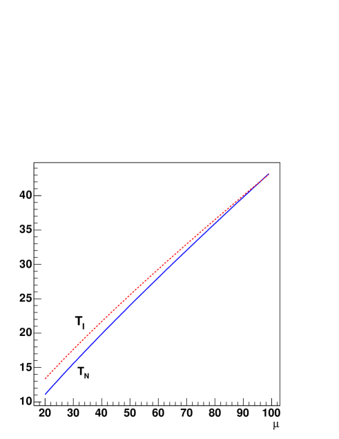
Figure 4: More details for the tensions at small and large values of $\mu$. The solid line $T_{N}$ at both pictures corresponds to the numeric result for the tension of $Z_{2}$ string, dashdoted line $T_{BPS}$ at the top picture is the tension of BPS string, while the dashed line $T_{I}$ at the bottom picture corresponds to extreme type I string.

The dependence of the string tension $T$ (3.16) on $m_{3}$ is shown at fig. 3, where we plotted dimensionless quantity $\frac{g^{2}}{2\pi m^{2}}\,T$ versus the ratio $\mu={m_{3}\over m}$. The numeric result ”interpolates” between the tension of the BPS string (3.12) near the origin and the tension (3.23) of the extreme type I string in the large $m_{3}$ limit. Indeed, we see from fig. 3 (and more details at fig. 4) that at small $\mu$ (small $m_{3}$) the tension of $Z_{2}$ string goes very close to the linear dependence of the BPS string tension of ${\cal N}=2\;$QED (3.4), truncated according to eq. (3.8). In particular, even at $\mu=1$ the difference of tensions of these two strings is about ten percent. Note also that the tension of $Z_{2}$ string is always smaller then the BPS bound, in accordance with the expected [7] type I superconductivity in ${\cal N}=2\;$QED (3.4). Moreover, at large $\mu$ or $m_{3}\gg m$ the tension of the $Z_{2}$ string in our numeric solution becomes indeed very close to the tension of extreme ANO string of type I, given by the logarithmic formula (3.23); one can see this in the region of large $\mu={m_{3}\over m}$ at fig. 3 and in more details at fig. 4.

4 Non-Abelian strings

When $m_{3}$ approaches $m$ the theory acquires additional symmetry. In this case the scalar VEV’s take the form (2.8), which respect the global combined color-flavor symmetry (2.9). On the other hand, the string solution (3.18) itself is not invariant under this symmetry. This means that applying rotation (2.9) we generate the whole class of string solutions with the same tension. In other words the symmetry (2.9) generates orientational zero modes of the string. Namely, embedding the Abelian $Z_{2}$-string (3.18) into the non-Abelian theory via (3.2) and applying the combined color-flavor rotation, one gets

$$\Phi_{A}^{a}=O\left(\begin{array}[]{ccc}\frac{g}{\sqrt{2}}\phi&0&0\\ 0&\frac{g}{\sqrt{2}}\phi&0\\ 0&0&a_{0}\end{array}\right)O^{-1}=\frac{g}{\sqrt{2}}\phi\delta^{a}_{A}+n_{a}n_{A}\left(a_{0}-\frac{g}{\sqrt{2}}\phi\right),$$

$$\begin{array}[]{c}A^{a}_{i}=n_{a}\;\frac{\varepsilon_{ij}x_{j}}{r^{2}}\,f(r),\ \ \ \ i,j=1,2,\end{array}$$ (4.1)

where we introduced the the unit orientation vector $n_{a}$ as

$$\begin{array}[]{c}n_{a}=O^{a}_{b}\delta^{b3}=O^{a}_{3}.\end{array}$$ (4.2)

The solution (4.1) interpolates between Abelian $Z_{2}$ string (3.18) for which ${\vec{n}}=(0,0,1)$ and anti-string with ${\vec{n}}=(0,0,-1)$.

We see that the flux of the string is determined now by an arbitrary vector $n_{a}$ in the color space. This makes our string really non-Abelian. As soon as the symmetry $O(3)_{C+F}$ is not broken in the vacuum, the rotations in (4.1) do not correspond to any gauge generators ”eaten” by the Higgs mechanism, these rotations indeed correspond to the physical orientational zero modes of the non-Abelian string. To verify this, one can explicitly construct the gauge invariant $n_{a}$-dependent operators.

As an example, consider the “non-Abelian” field strength (to be denoted by bold letters) [45, 13],

$$\begin{array}[]{c}({\bf{F}}_{3}^{*})_{AB}=\frac{2}{m^{2}}\,\varepsilon^{abc}\bar{\Phi}_{A}^{a}F_{3}^{*b}\Phi^{c}_{B}\,,\end{array}$$ (4.3)

where the subscript 3 marks the $z$-axis, of direction of the string, and $F_{3}^{*a}={\textstyle{1\over 2}}\varepsilon_{ij}F^{a}_{ij}$; it is by definition gauge invariant. Eq. (4.1) implies that on string solution

$$\begin{array}[]{c}({\bf{F}}_{3}^{*})_{AB}=\varepsilon_{ABc}n_{c}\,\frac{g^{2}\phi^{2}}{m^{2}}\,\frac{1}{r}\,\frac{df}{dr}\,.\end{array}$$ (4.4)

¿From this formula we readily infer the physical meaning of the orientational moduli $\vec{n}$: the direction of the flux of the color-magnetic field (defined in the gauge-invariant way, see (4.3)) in the flux tube is determined by $n_{a}$. For Abelian strings (3.18) only the component with $A,B=1,2$ of the color-magnetic flux does not vanish.

Our analysis in this section is almost parallel to constructions in ref. [11] where non-Abelian strings were found in ${\cal N}=2\;$SQCD with the gauge group $SU(2)\times U(1)$. However, the essential difference is that strings of ref. [11] topologically exist due to winding around the $U(1)$ factor of the gauge group, more precisely they are associated with $\pi_{1}(SU(2)\times U(1)/Z_{2})=Z$. Therefore, one can say that these strings are Abelian in the sense of their Abelian topological origin. Still, they are non-Abelian in the sense of the presence of orientational zero modes associated with the rotation of the string flux inside the gauge group.

In contrast, our strings here are associated with $\pi_{1}(SO(3))=Z_{2}$. Therefore they are non-Abelian both in the sense of their non-Abelian winding and in the sense of the presence of orientational zero modes.

5 Effective world sheet theory

In this section we consider the low energy effective theory on the string world sheet associated with ”slow” dynamics of orientational zero modes. We will find that the orientational zero modes are effectively described by two-dimensional $O(3)$ sigma model. However, unlike the BPS case of refs. [14, 11, 13, 30], the sigma model appearing here is non-supersymmetric, and this leads to different physical properties of our four-dimensional theory.

5.1 Kinetic term

Assume that the orientational collective coordinates $n_{a}$ are slow varying functions of the string world-sheet coordinates $x_{k}$, $k=0,3$. Then, moduli $n_{a}$ become the fields on the world sheet of a two-dimensional sigma model. Since the vector $n_{a}$ parametrizes the string zero modes, there is no potential term in this sigma model. We begin with the kinetic term (cf. with [11, 13]).

To obtain the kinetic term let us substitute the solution (4.1), depending upon the moduli $n_{a}$, into the action (2.4) assuming that the fields acquire a dependence on the ”slow” coordinates $(t,z)$ via $n_{a}(t,z)$. Technically it is convenient to work with the solution (4.1) in the singular gauge, and proceeding to this gauge we immediately find that we should modify the solution.

Indeed, the solution (4.1) was obtained as an $O(3)_{C+F}$ rotation of the Abelian string (3.18). Now we make this rotation locally (i.e. depending on $(t,z)$), therefore, the $(t,z)$ components of gauge potential $(A_{0},A_{3})$ do not necessarily vanish, and they should be added to the ansatz. This situation is quite familiar (see e.g. [38, 42, 11]), since one routinely encounters it in the soliton studies.

To begin with, let us rewrite the $O(3)_{C+F}$ rotation in $SU(2)$-terms, using the representation

$$\begin{array}[]{c}O^{ab}=\frac{1}{2}{\rm Tr}\left(\tau^{a}U\tau^{b}U^{-1}\right).\end{array}$$ (5.1)

It is easy to check that vector $n_{a}$ satisfies the relation

$$\begin{array}[]{c}n_{a}\tau^{a}=U\tau^{3}U^{-1}.\end{array}$$ (5.2)

Next, we propose an ansatz for the $k=0,3$ components of the gauge potential

$$\begin{array}[]{c}A_{k}^{a}\tau^{a}=-2i\,\left(\partial_{k}U\right)\,U^{-1}\,\rho(r)\,,\qquad k=0,3\,,\end{array}$$ (5.3)

where a new profile function $\rho(r)$ (depending only upon the transverse radius $r=\sqrt{x_{1}^{2}+x_{2}^{2}}$) is introduced. In terms of the moduli fields $n_{a}$ one can write

$$\begin{array}[]{c}A_{k}^{a}=-\varepsilon^{abc}\,n_{b}\,\partial_{k}n_{c}\,\rho(r)\,.\end{array}$$ (5.4)

using a particular choice for the matrix $U\in SU(2)$ (satisfying ${\rm Tr}\left(\tau^{3}U^{-1}\partial_{k}U\right)=0$), which is not uniquely defined by a vector ${\vec{n}}\in SU(2)/U(1)$ [13].

The profile function $\rho(r)$ in (5.4) is determined through a minimization procedure (cf. [38, 42]) which generates a separate equation of motion for $\rho$. The kinetic term for $n_{a}$ comes from the gauge and matter kinetic terms in (2.4). Using (4.1) and (5.4), we find for the $k=0,3$, $i=1,2$ components of the $SU(2)$ gauge field strength

$$\begin{array}[]{c}F_{ki}=\frac{\tau^{a}}{2}\left(\partial_{k}n_{a}\,\frac{\varepsilon_{ij}x_{j}}{r^{2}}\,f\left(1-\rho\right)+\varepsilon^{abc}n_{b}\partial_{k}n_{c}\,\frac{x_{i}}{r}\,\,\frac{d\rho}{dr}\right).\end{array}$$ (5.5)

We see that in order to get a finite contribution from ${\rm Tr}\ F_{ki}^{2}$ in the action one has to impose

$$\begin{array}[]{c}\rho(0)=1\end{array}$$ (5.6)

and also $\rho(r)$ should vanish at infinity

$$\begin{array}[]{c}\rho(\infty)=0.\end{array}$$ (5.7)

Substituting (5.5) into the action (2.4) and including, in addition, the kinetic term for adjoint matter, we arrive at

$$\begin{array}[]{c}S^{(1+1)}=\frac{\beta}{2}\,\int dt\,dz\,\left(\partial_{k}\,n_{a}\right)^{2}\,,\end{array}$$ (5.8)

where the sigma-model coupling constant $\beta$ is given by the normalization integral

$$\begin{array}[]{c}\beta=\frac{2\pi}{g^{2}}\,\int_{0}^{\infty}rdr\left[\left(\frac{d\rho}{dr}\right)^{2}+\frac{1}{r^{2}}\,f^{2}\,\left(1-\rho\right)^{2}+\right.\\ +\left.2\left(a_{0}(1-\rho)-\frac{g}{\sqrt{2}}\phi\right)^{2}+2\left(a_{0}-\frac{g}{\sqrt{2}}\phi(1-\rho)\right)^{2}\right].\end{array}$$ (5.9)

The functional (5.9) must be minimized with respect to $\rho$ with the boundary conditions given by (5.7), (5.6). Varying (5.9) with respect to $\rho$ one readily obtains the second-order equation which the function $\rho$ must satisfy,

$$\begin{array}[]{c}-\frac{d^{2}\rho}{dr^{2}}-\frac{1}{r}\,\frac{d\rho}{dr}-\frac{1}{r^{2}}\,f^{2}\left(1-\rho\right)+2\rho\left(a_{0}^{2}+\frac{g^{2}}{2}\phi^{2}\right)-2\left(a_{0}-\frac{g}{\sqrt{2}}\phi\right)^{2}=0.\end{array}$$ (5.10)

Taking into account this equation we rewrite the sigma model coupling (5.9) as

$$\begin{array}[]{c}\beta=\frac{2\pi}{g^{2}}\,I,\end{array}$$ (5.11)

where normalization integral $I$ is given by

$$\begin{array}[]{c}I=2\int^{\infty}_{0}rdr\;\left[\left(a_{0}-\frac{g}{\sqrt{2}}\phi\right)^{2}+\sqrt{2}g\rho\phi a_{0}\right].\end{array}$$ (5.12)

We see that the two-dimensional coupling constant is determined by the four-dimensional non-Abelian coupling. This is quite similar to what was observed for BPS non-Abelian string in [13].

We solve eq. (5.10) numerically using the numeric solutions for the string profile functions, see Sect. 3.4. The result for $\rho$ is shown at fig. 5. Note that the first derivative of $\rho$ does not vanish at $r=0$ similar to the BPS case, see [11]. Substituting the solution for $\rho$ in (5.12) we find

$$\begin{array}[]{c}I\simeq 0.78\end{array}$$ (5.13)

Note that in the BPS case the similar normalization integral is equal to one [13]. The explanation of this is related to equality of the monopole mass on the Coulomb branch to the one in the confinement phase present for the case of BPS strings [13, 30]. In the theory at hand we don’t have such an equality as we will explain in Sect. 6.

Figure 5: Numeric solution for the profile function $\rho$.

In summary, the effective world-sheet theory describing dynamics of the string orientational zero modes is $O(3)$ sigma model. The symmetry of this model reflects the presence of the global $O(3)_{C+F}$ symmetry in the microscopic theory. The coupling constant of this sigma model is determined by minimization of the action (5.9) for the profile function $\rho$. The minimal value of $I$ is given by (5.13).

Clearly, the action (5.8) describes the low-energy limit. In principle, the zero-mode interaction has higher derivative corrections which run in powers of

$$\begin{array}[]{c}\frac{\partial}{m}\,,\end{array}$$ (5.14)

where $m$ gives the order of magnitude of masses of the gauge/matter multiplets in our microscopic $O(3)$ theory. The sigma model (5.8) is adequate at scales below $m$ where higher-derivative corrections are negligibly small.

The same scale $m^{-1}$ determines the thickness of the strings we deal with. In other words, the effective sigma model action (5.8) is applicable at the length scales above $m^{-1}$, which, thus, plays the role of an ultraviolet cutoff for the model (5.8).

5.2 $m_{3}\neq m$

To facilitate contact between the microscopic and macroscopic theories, it is instructive to start from a deformed microscopic theory so that the string orientational moduli are lifted already at the classical level. Thus, let us drop the assumption $m_{3}=m$ and introduce a small mass difference. We will assume that

$$\begin{array}[]{c}\Delta m\equiv\left|m_{3}-m\right|\ll m\,.\end{array}$$ (5.15)

At $m_{3}\neq m$ the flavor (global) $O(3)$ symmetry of the microscopic theory is explicitly broken down to $O(2)\cong U(1)$ (corresponding to rotations around the third axis in the $SU(2)/U(1)$ coset space). Correspondingly, the moduli of the non-Abelian string are lifted, i.e. the sigma-model acquires some mass terms.

Let us derive the effective two-dimensional world sheet theory for the case of $m_{3}\neq m$. As already discussed in Sect. 3.2, the solutions of the equations of motion (3.14) with the minimal windings $n=\pm 1$ directly correspond to the $Z_{2}$ string and anti-string. Note that both equations of motion (3.14) and boundary conditions (3.15) are written for arbitrary $m$ and $m_{3}$; the solution for the $Z_{2}$ string is written in terms of the profile functions in (3.18), while the solution for the $Z_{2}$ anti-string can be obtained from (3.18) by $f\to-f$.

At small $\Delta m$ one can still introduce the orientational quasi-moduli $n_{a}$. In terms of the effective two-dimensional world sheet theory $\Delta m\neq 0$ leads to a shallow potential for the quasi-moduli $n_{a}$. The two minima of the potential at $n=\{0,0,\pm 1\}$ would correspond directly to the $Z_{2}$ string and anti-string.

Let us derive this potential in the leading approximation in $\Delta m$, this can be done just by substituting the string solution (4.1) into the potential in the action (2.4). Keeping the linear in $\Delta m$ terms, one gets

$$\begin{array}[]{c}S^{(1+1)}=\frac{\beta}{2}\,\int dt\,dz\,\left(\left(\partial_{k}\,n_{a}\right)^{2}\,+\gamma m_{0}\Delta m(1-n^{2}_{3})+{\rm const}\right),\end{array}$$ (5.16)

where $m_{0}={\textstyle{1\over 2}}(m+m_{3})$ while the constant $\gamma$ is given by the ratio

$$\begin{array}[]{c}\gamma=\frac{I_{1}}{I}\simeq 0.8,\end{array}$$ (5.17)

where $I$ is the normalization integral (5.12), with the numeric value (5.13), while

$$\begin{array}[]{c}I_{1}=4\int_{0}^{\infty}rdr\left|a_{0}^{2}-\frac{g^{2}}{2}\phi^{2}\right|\end{array}$$ (5.18)

and after substituting the numeric results for the profile functions (see Sect. 3.4) into (5.18) one finds

$$\begin{array}[]{c}I_{1}\simeq 0.63\end{array}$$ (5.19)

Note, that in linear in $\Delta m$ approximation we do not need to modify the string solution (4.1), since, as usually, corrections to the string solution contribute only in the quadratic in $\Delta m$ order, due to equations of motion, and in this approximation, the integral (5.18) was calculated, putting $m_{3}=m$.

To extract the $(\Delta m)^{2}$ corrections to the potential in (5.16) one has to modify the string solution introducing a new profile function like it is done in [13] for the case of BPS string. We have checked that already in $(\Delta m)^{2}$ order the potential has a complicated $n_{3}$-dependence: generally it contains an infinite series in powers of $(1-n^{2}_{3})$.

The theory in (5.16) is massive deformation of the $O(3)$ sigma model. The potential in (5.16) is similar to the one arising in the case of non-Abelian BPS strings, see [29, 13, 30]; however, the difference is that for the BPS case the potential appears only at the quadratic order in $\Delta m$ while in (5.16) it arises already in linear order. The reason is that in the BPS case the world sheet theory has ${\cal N}=2\;$supersymmetry and the (twisted) superpotential is proportional to $\Delta m$, that ensures the bosonic potential proportional to $(\Delta m)^{2}$. Note, that the non-analytic dependence of the potential in (5.16) on the mass difference $\Delta m=\left|m_{3}-m\right|$ cannot appear in supersymmetric sigma model.

5.3 Fermionic zero modes

As we already explained in Sect. 2 in the ${\cal N}=2\;$limit of small $m_{3}$ our string solution is 1/2-BPS saturated. This means that, four charges (out of the eight supercharges of the four-dimensional ${\cal N}=2\;$algebra) act on the string solution (3.9) trivially, while the remaining four charges generate the four fermionic zero modes (called supertranslational, since they are superpartners to the two translational bosonic zero modes). The corresponding four fermionic moduli are superpartners to the coordinates $(x^{(0)}_{1},x^{(0)}_{2})$ of the ”string center”, and the four SUSY charges, vanishing on the BPS string solution, turn (after we consider moduli as slow functions of the world sheet co-ordinates $(z,t)$) into the four generators of the two-dimensional ${\cal N}=2$ supersymmetry algebra; the supertranslational fermionic zero modes for the $U(1)$ ANO string in were studied in [7].

As we increase $m_{3}$, the ${\cal N}=2\;$supersymmetry breaks down to ${\cal N}=1\;$, and the string solution is no longer BPS-saturated. Still the number of the fermionic zero modes does not jump: all four generators of the ${\cal N}=1\;$SUSY algebra act now non-trivially on the solution and, therefore, produce the same number of the ”supertranslational” (do not have, in fact, any supersymmetry in the world sheet theory at $m_{3}\neq 0$) fermionic zero modes [7]. These ”supertranslational” modes decouple from the internal dynamics and they are not essential for our purposes below.

Approaching the point $m_{3}=m$, our theory acquires an additional symmetry (2.9), responsible for appearance of orientational zero modes of the string, described by the $O(3)$ sigma model (5.8). As we already mentioned, one should not expect world sheet supersymmetry at $m_{3}\neq 0$, and nothing special happens at the point $m_{3}=m$: supersymmetry is still absent in the world sheet theory. Therefore, we do not expect any ”superorientational” fermionic zero modes to appear at the point $m_{3}=m$, and we expect that the internal string dynamics is described by the non-supersymmetric version of the $O(3)$ sigma model (5.8). This is extremely important for the physical conclusions of the Sect. 6 below.

Note, that the properties of the world sheet theory we consider are essentially different from the case of non-Abelian strings, considered in [11, 13]. For that non-Abelian BPS string four supercharges act trivially on the string solution and turn into the SUSY generators in the effective world sheet theory. The four ”superorientational” fermionic zero modes were found in [13], the corresponding four fermionic moduli are superpartners of bosonic variables $n_{a}$ in the effective world sheet ${\cal N}=2\;$$O(3)$ sigma model. It is also useful to notice, that the world-sheet supersymmetry imposes serious restrictions to the possible form of the potential in the massive deformation of the sigma-model, while our conclusions of Sect. 5.2 rather point out that the potential in (5.16) ( as well as generic form of corrections arising beyond the linear approximation in $\Delta m$) is inconsistent with the world-sheet supersymmetry.

6 World sheet dynamics

In the previous section we show that the internal world sheet dynamics of our non-Abelian string is described in terms of the (massive deformation of) $O(3)$ sigma model. Although this theory is asymptotically free and runs into strong coupling regime its physics is well understood. In this section we review some known results about $O(3)$ sigma model and interpret them in terms of strings in four-dimensional ${\cal N}=1$^∗ theory.

6.1 Quasiclassical limit

Let us start with the case of massive $O(3)$ sigma model at $m_{3}\neq m$. The sigma model (5.16) is asymptotically free [46]; at large distances (low energies) it gets into the strong coupling regime. The running coupling constant as a function of the energy scale $E$ at one-loop is given by

Figure 6: Beta-function of four-dimensional (microscopic) and two-dimensional (macroscopic) theory. At energies $E\gg m$ the coupling does not run due to conformal invariance of ${\cal N}=4$ theory and equals to some bare value $g_{0}$. At the scales below $m$ the running of coupling is determined by two-dimensional world-sheet theory and goes towards the strong-coupling regime.

$$\begin{array}[]{c}4\pi\beta=4\ln{\left(\frac{E}{\Lambda_{\sigma}}\right)}+\cdots,\end{array}$$ (6.1)

where $\Lambda_{\sigma}$ is the dynamical scale of the sigma model. As was mentioned previously, the ultraviolet cut-off of the sigma model at hand is determined by $m$. At this UV cut-off scale Eq. (5.11) holds. Hence,

$$\begin{array}[]{c}\Lambda^{4}_{\sigma}=m^{4}e^{-\frac{8\pi^{2}}{g^{2}}\,I}.\end{array}$$ (6.2)

Note that in the microscopic theory, due to the VEV’s of the squark fields, the coupling constant is frozen at $m$. There are no logarithms in microscopic theory neither above this scale (because of conformal invariance of ${\cal N}=4\;$theory) nor below it, however below $m$ the logarithms of the macroscopic theory take over, see fig. 6.

Consider, first, the $O(3)$ sigma model in the quasiclassical regime of large $\Delta m$; to be more precise take $\Delta m\gg\Lambda_{\sigma}$ (note that we always assume that $\Delta m\ll m$). The coupling constant of the $O(3)$ sigma model is frozen at $\Delta m$. Therefore in the region of large $\Delta m$, $\Delta m\gg\Lambda_{\sigma}$ the inverse coupling $\beta$ is large and we can study the model in the quasiclassical approximation.

The potential of the $O(3)$ sigma model is derived in Sect. 5.2 and the result is schematically presented at fig. 7. This potential is very similar to the potential in the case of BPS non-Abelian string, and the analysis below will be rather close to those presented in [29, 13, 30].

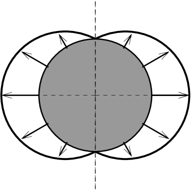
Figure 7: The meridian slice of the target space sphere ${\vec{n}}\in S^{2}$ of the $O(3)$ sigma-model. Arrows present the scalar potential in (5.16), with their lengths being the strength of the potential. Two vacua of the model are seen at the north and south poles $n_{3}=\pm 1$ of the sphere.

The potential has two vacua at the north ($n_{3}=1$) and south ($n_{3}=-1$) poles. These vacua correspond to Abelian $Z_{2}$-string and anti-string, see (3.13). There is a sigma model kink (domain wall in the world sheet theory), interpolating between two vacua of massive $O(3)$ sigma model. This kink is interpreted as a monopole which provides a junction of the $Z_{2}$-string and anti-string. Remember that monopole has magnetic charge one while $Z_{2}$-string and anti-string have charges $\pm 1/2$; therefore the string cannot end on a monopole (and this is a reason for the stability of $Z_{2}$-strings), and a monopole can appear only as a junction of $Z_{2}$-string and anti-string. Note also, that in the Higgs vacuum monopoles do not exist as a free states. They are in the confinement phase, attached to ANO strings carrying their magnetic fluxes.

The similar identification of a two-dimensional sigma model kink as confined four-dimensio-nal monopole was presented in refs. [29, 13, 30] for the case of BPS monopoles, and a lot of arguments was presented in favor of this interpretation. In particular, in [13] the first order equations for the 1/4-BPS string junction were explicitly solved and the solution was shown to be determined in terms of the kink solution of massive $O(3)$ sigma model. Moreover, the masses of four-dimensional monopole and two-dimensional kink were shown to coincide for these solutions .

Here we do not have explicit analytic solutions, but we will use this identification to calculate the mass of monopole in the confinement phase. First, rewriting the action (5.16) in the holomorphic representation upon stereographic projection, one gets

$$\begin{array}[]{c}S^{(1+1)}=2\beta\,\int dt\,dz\,\frac{\left|\partial_{k}\,w\right|^{2}\,+\gamma m_{0}\Delta m|w|^{2}}{(1+|w|^{2})^{2}},\end{array}$$ (6.3)

where $w$ is a complex field. Two classical vacua are now located at $w=0$ (north pole) and $w=\infty$ (south pole). Note that the model (6.3) has $U(1)$ symmetry $w\to e^{i\theta}w$, since the potential of massive deformation of the sigma model (5.16), as we already mentioned, does not break $O(3)_{C+F}$ completely, leaving $U(1)$-rotations do not acting on $n_{3}$.

The kink solution, interpolating between two classical vacua is now easy to find. It is a static solution depending only on the coordinate $z$. In one-dimensional case the equations of motion can be always integrated by energy conservation law, and for the kink in (6.3) we get the first-order equation

$$\begin{array}[]{c}\partial_{z}w=-\sqrt{\gamma m_{0}\Delta m}\,w\end{array}$$ (6.4)

with the solution, given by

$$\begin{array}[]{c}w(z)=\exp\left(-\sqrt{\gamma m_{0}\Delta m}\,(z-z_{0})-i\theta\right).\end{array}$$ (6.5)

Here $z_{0}$ is the center of kink, while $\theta$ is an arbitrary phase; in fact, these two parameters enter only in the combination $\sqrt{\gamma m_{0}\Delta m}z_{0}-i\theta$, so that the notion of the kink center gets complexified.

Now, substituting the kink solution into the action (6.3), one gets the mass of the kink

$$\begin{array}[]{c}M_{\rm kink}=2\beta\sqrt{\gamma m_{0}\Delta m}.\end{array}$$ (6.6)

As we already explained, the kink mass (6.6) should be identified with the mass of the confined monopole providing a junction of $Z_{2}$-string and anti-string. Expressing the kink mass in terms of parameters of four-dimensional theory, using (5.11) and (5.17), one gets the mass of confined monopole

$$\begin{array}[]{c}M_{\rm m}^{\rm conf}=\frac{4\pi}{g^{2}}\sqrt{m\Delta m\,I_{1}I}\left(1+O\left(\frac{\Delta m}{m}\right)\right).\end{array}$$ (6.7)

with the numeric coefficient $\sqrt{I_{1}I}\simeq 0.7$ (see (5.13) and (5.19)). On the Coulomb branch at $m_{3}=0$, the monopole mass is given by the Seiberg-Witten formula, which in the weak coupling regime reads

$$\begin{array}[]{c}M_{\rm m}^{\rm Coulomb}=\frac{4\pi}{g^{2}}\,m.\end{array}$$ (6.8)

Comparing two results (6.7) and (6.8) for the monopole masses, one finds that when moving into the Higgs phase by increasing $m_{3}$, the monopole confines and its mass decreases: given at small $\Delta m$ by (6.7). Classically, in the non-Abelian point $m_{3}=m$ it vanishes, while the monopole size becomes infinite; however, in the next section we find, that this does not happen in quantum theory, due to the (two-dimensional) non-perturbative instanton effects on the string world sheet.

To conclude this section, let us discuss the physical meaning of extra modulus $\theta$ of the kink solution (6.5). There is a continuous family of solitons, interpolating between the north and south poles of the target space sphere, see fig. 7. The soliton trajectory can follow any meridian, due to unbroken $U(1)$ symmetry. After quantization, the phase $\theta$ leads to the whole tower of ”dyonic” states [48, 49] with the non-zero charge with respect to unbroken $U(1)$ symmetry.

6.2 Quantum limit

In this section we consider the quantum theory at $\Delta m\to 0$. As we already discussed, the non-Abelian string in ${\cal N}=1$^∗ theory is a non BPS string, and therefore its world sheet dynamics is described in terms of the non supersymmetric $O(3)$ sigma model (5.8). Now, let us review the known results on the $O(3)$ sigma model and interpret them in terms of strings and monopoles in our original four dimensional theory.

The exact spectrum of the non-supersymmetric $O(3)$ sigma model was found long ago in [50]. Moreover, it was shown in ref. [51] that the main features of the exact solution can be qualitatively understood in terms of the $1/N$ expansion of $CP^{N-1}$ models, if one formally puts $N=2$ . It turns out that the dynamics of the $O(3)$ sigma models for supersymmetric and non-supersymmetric cases are rather different. Below we remind these differences, which lead to quite different properties of the non-Abelian non-BPS strings from the BPS strings studied in [13].

In the $CP^{1}$ formulation the action of the $O(3)$ sigma model (5.8) reads

$$\begin{array}[]{c}S_{O(3)}=\frac{\beta}{2}\int dtdz|{\cal D}_{k}Z_{l}|^{2},\end{array}$$ (6.9)

where $Z_{i}$ is the complex doublet of $SU(2)$, constrained by $\sum_{l}|Z_{l}|^{2}=1$, while the covariant derivative ${\cal D}_{k}=\partial_{k}-i{\cal A}_{k}$ contains a two dimensional non-dynamical $U(1)$ gauge field ${\cal A}_{k}$. This is a particular case of the $CP^{N-1}$ model, where in the action (6.9) $Z_{l}$ should be treated as $N$-component complex field in the fundamental representation of $SU(N)$. The $1/N$-expansion yields two main results [51]: the field $Z_{i}$ acquires a mass of order of $\Lambda_{\sigma}$, and the $U(1)$ gauge field ${\cal A}_{k}$ acquires at one loop level the standard kinetic term.

Classically the vector $n_{a}$ can be directed anywhere on the sphere $S^{2}$, so one naively expects the spontaneous breaking of the $SU(2)$ symmetry and the massless Goldstone modes. However, the first of the observations above shows, that the spontaneous $SU(2)$ symmetry breaking does not occur in quantum theory and there are no massless particles. The second result implies confinement for $Z_{l}$ fields [51]. The reason is that the Coulomb potential between two charges in two dimensions is linear in the distance between these charges

$$\begin{array}[]{c}V_{\rm Coulomb}^{\rm 2d}=\Lambda^{2}_{\sigma}|z_{1}-z_{2}|,\end{array}$$ (6.10)

where $z_{1}$ and $z_{2}$ are positions of the charges. In fact, the exact spectrum of $O(3)$ sigma model [50] contains one triplet, which is interpreted as $\bar{Z}Z$-meson in the adjoint representation of global $SU(2)$.

Before interpreting these results in terms of strings and monopoles in four dimensional theory, let us remind the similar results for the ${\cal N}=2\;$supersymmetric $O(3)$ sigma model [51]. The presence of the world-sheet fermions drastically changers the above outlined picture. The fermions generate a mass of the order of $\Lambda_{\sigma}$ for the $U(1)$ gauge field via the anomalous one loop diagram. Thus, the linear potential (6.10) is screened and there is no confinement, in accordance with the exact spectrum of ${\cal N}=2\;$$O(3)$ sigma model, which contains doublets of $SU(2)$, interpreted as massive $Z_{l}$ particles.

In fact, in the ${\cal N}=2\;$$O(3)$ sigma model there are two vacua, and this is easy to understand. One can start with massive deformation of the sigma model in quasiclassical regime, like we did in previous section (cf. also with [48, 13]). Then two vacua are just the north and south poles at fig. 7, corresponding, as we know, to two elementary Abelian strings with minimal windings in four dimensions. When we reduce the mass parameter $\Delta m$ the number of vacua in supersymmetric version of the model does not change due to the Witten index [55]. Thus, in massless case we still have two quantum vacua in the supersymmetric sigma model, to be interpreted as two elementary non-Abelian strings [13]. The order parameter to distinguish between these two vacua is the bifermionic condensate generated by instantons [56].

As soon as we have two vacua at $\Delta m=0$ we still have a kink (in fact two kinks [54]) interpolating between them. This kink is interpreted as a quantum version of the non-Abelian monopole, providing 1/4-BPS string junction between two elementary strings. Classically this monopole would have infinite size and zero mass, but this does not happen in quantum theory. There is no massless states in $O(3)$ sigma model, therefore the kink/monopole has finite size (of the order of $\Lambda_{\sigma}^{-1}$) and non-vanishing mass (of the order of $\Lambda_{\sigma}$), given by the anomalous term in ${\cal N}=2\;$superalgebra [13]. The kink of ${\cal N}=2\;$$O(3)$ sigma model is a doublet of global $SU(2)$ and can be interpreted as a $Z_{l}$-particle in the $CP^{1}$ formulation (6.9) [51], see also [54]. Thus, we conclude that confined non-Abelian BPS monopoles are associated with the $Z_{l}$ fields in the two-dimensional world sheet $CP^{1}$ sigma model.

Now let us return to our case of the non BPS string, described by non supersymmetric $O(3)$ sigma model. First, in the $O(3)$ sigma model there is the only vacuum state, and therefore the only non-Abelian string with minimal tension in four dimensional theory. Second, as soon as there are no different vacuum states in the world-sheet theory, there is no room for the kinks interpolating between them. Hence, there is no non-Abelian monopoles in the limit $\Delta m=0$; where do they disappear?

First, the absence of two elementary strings is easy to understand. Due to mixing, two vacua of the $O(3)$ sigma model present at large $\Delta m$ are split, and in the limit $\Delta m=0$ we end up with two energy levels with the energy gap of the order of $\Lambda_{\sigma}$. Thus we do have the only one non-Abelian string with minimal tension, the other tension is larger. Note, that the splitting of the order of $\sim\Lambda^{2}_{\sigma}$ is rather small, compare to the classical tension of each string ($\sim m^{2}/g^{2}$).

Still, one can have junction of the ”minimal” string with the exited string, and this junction should be again interpreted as a non-Abelian monopole. However, since the exited string carries more energy, one would expect that a monopole comes together with an anti-monopole in a meson-like configuration, see fig. 8. The total energy of such object is determined by length of the exited string between monopole and anti-monopole times the tension difference between two lightest strings. This gives the energy $\sim\Lambda^{2}_{\sigma}|z_{1}-z_{2}|$, where $z_{1}$ and $z_{2}$ are positions of monopole and anti-monopole, or we immediately recognize the confining potential (6.10).

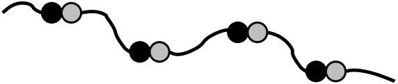
Figure 8: Two-dimensional confinement of monopoles (black dots) and anti-monopoles (grey dots) on the string.

As we already mentioned, the $O(3)$ sigma model kink is interpreted as a $Z_{l}$-particle in the $CP^{1}$ description. In (non supersymmetric) $O(3)$ sigma model the $Z_{l}$-particles are confined. Now we see, that the above conclusion that monopole and anti-monopole form a meson-like configuration on the string (see fig. 8) is in a complete accordance with known results about the confinement of $Z_{l}$-particles/kinks in the $O(3)$ sigma model.

Since kinks (or the $Z_{l}$-particles) of the $O(3)$ sigma model are in the doublet representation of the global unbroken $SU(2)_{C+F}$, the kink-anti-kink meson can be either scalar or triplet of $SU(2)_{C+F}$. Clearly, the scalar is unstable, because kink and anti-kink with the ”opposite” quantum numbers can annihilate each other. However, they cannot annihilate each other when forming a triplet state and, as we already mentioned, the exact spectrum of $O(3)$ model indeed consists of the stable massive triplets of $SU(2)_{C+F}$ [50]. In four dimensions these states correspond to the (attached to the string) stable monopole-anti-monopole mesons in the triplet representation of the unbroken $SU(2)_{C+F}$.

To avoid confusion we would like to stress that monopoles are in the confinement phase in the Higgs vacuum we consider in this paper. This four-dimensional confinement implies that monopoles do not exist as free states, but they are attached to strings carrying magnetic flux. We see now, that on top of this four-dimensional confinement, we have an ”extra” two-dimensional confinement in the $O(3)$ sigma model, which additionally forces monopoles and anti-monopoles to form a meson-like configuration on the string they are attached to (see fig. 8).

7 Conclusions

In this paper we presented a simplest model for the non-Abelian strings. We have considered the ${\cal N}=4$ supersymmetric $SU(2)$ gauge theory, perturbed by the mass terms for the chiral multiplets, in the Higgs vacuum. We have shown that at the special value of mass parameters $m_{3}=m$ the theory has an unbroken global $O(3)_{C+F}$ symmetry, responsible for the appearance of orientational zero modes of the $Z_{2}$ strings, associated with the rotation of their color fluxes inside the $SU(2)$ group. The presence of these zero modes makes the $Z_{2}$ strings non-Abelian.

We have worked out the effective theory on the world sheet of the non-Abelian string. It turn out to be the two-dimensional (non-supersymmetric) $O(3)$ sigma model. Then we have translated the results for the $O(3)$ sigma model to the physics of strings in four dimensions. Like in [29, 13, 30], the confined ’t Hooft-Polyakov monopole is identified with the kink of two-dimensional $O(3)$ sigma model, and this allowed us to calculate its mass. In particular, we demonstrated that besides the four dimensional confinement, which ensures that monopole is a $Z_{2}$-string junction, the monopoles are also confined in the two-dimensional sense. Namely, monopoles and anti-monopoles form meson-like configuration on the string they are attached to. The spectrum of the theory contains these stable monopole-anti-monopole mesons in the triplet representation of $O(3)_{C+F}$.

Since there are no experimental signs for ”Abelization” in the real world QCD, it is plausible to expect that the non-Abelian strings, like we discussed here and in [14, 11], can be also responsible for the confinement there. The orientational modes of the non-Abelian string appear due to the presence of unbroken global color-flavor symmetry ($O(3)_{C+F}$ in the model considered above) and ensure the ”de-Abelization” of the string.

All results of this paper concern the Higgs vacuum at weak coupling, i.e. in the Higgs vacuum the color electric (adjoint) charges condense, giving rise to the non-Abelian magnetic strings and confinement of monopoles. However, it is well known that ${\cal N}=1$^∗ theory has the $SL(2,Z)$ duality group [57, 23]. In particular, the S-duality transformation was analyzed in [23] at small $m_{3}$, and it was shown that it exchanges the Higgs and monopole vacua. Thus, the confinement of monopoles in the Higgs vacuum is mapped to the confinement of W-bosons and quarks (if we introduce quarks) in the monopole vacuum.

Can we extrapolate this picture to large $m_{3}$? In particular, can we get the non-Abelian electric $Z_{2}$-strings in the monopole vacuum by S-duality transformation from the non-Abelian magnetic $Z_{2}$-strings in the Higgs vacuum? Unfortunately, this is hard to do. The duality transformations at arbitrary $m_{3}$ were studied in [58, 59], and it was shown that BPS-data like chiral condensates and domain wall tensions in the Higgs and monopole vacua are mapped one into another by S-duality. However, the strings we found are not BPS, they become BPS strings only in the ”Abelian” limit of small $m_{3}$ (and in this limit the Abelian quark confinement in the monopole vacuum is well understood [2, 5, 60, 7]). Therefore, it hard at the moment to make any conclusion on the existence and properties of $Z_{2}$-strings in the monopole vacuum just from S-duality. Moreover, the S-duality transformation maps small $g$ to large $1/g$. Thus, say, the Higgs vacuum at small $g$ is mapped to the monopole vacuum at large bare ${\cal N}=4\;$coupling, and this is not what can be analyzed by our methods. It would be nice to study the theory, starting from the small bare ${\cal N}=4\;$coupling (of course the running coupling at the monopole vacuum is always large).

Let us finally point out, that the $O(3)$ sigma model, which is a world-sheet theory for the effective string in the perturbed $SU(2)$ ${\cal N}=4$ theory near the color-flavor locked vacuum, is similar in certain aspects to the string ”spin” sigma-models, arising in the $SU(2)$ flavor sector of the ${\cal N}=4$ Yang-Mills theory in the context of the AdS/CFT correspondence [61]. At the moment the pictures for the effective and fundamental string sigma-models are still essentially different: the effective string sigma-model is not conformal and runs into strong coupling, where quantum effects change drastically the naive classical picture, while on the fundamental string sigma-model side only the predictions of the classical theory can be used in some cases. However, one can still hope that these two ways, when the world-sheet sigma-models arise in the supersymmetric Yang-Mills theory, are complementary realizations of the same phenomenon; the string/gravity dual of the ${\cal N}=1$^∗ theory itself was studied in [62].

References

-
[1]
G. t’ Hooft, in Proceed. of the Europ. Phys. Soc. 1975, ed. by
A.Zichichi (Editrice Compositori, Bologna, 1976) p. 1225.
S. Mandelstam, Phys. Rep. 23C 145 (1976);
A. Polyakov, Nucl. Phys. B120 (1977) 429. - [2] N. Seiberg and E. Witten, Nucl. Phys. B426, 19 (1994), (E) B430, 485 (1994) [hep-th/9407087].
- [3] N. Seiberg and E. Witten, Nucl. Phys. B431, 484 (1994) [hep-th/9408099].
-
[4]
A. Abrikosov, Sov. Phys. JETP 32 1442 (1957)
[Reprinted in Solitons and Particles, Eds. C. Rebbi and G. Soliani
(World Scientific, Singapore, 1984), p. 356];
H. Nielsen and P. Olesen, Nucl. Phys. B61 45 (1973) [Reprinted in Solitons and Particles, Eds. C. Rebbi and G. Soliani (World Scientific, Singapore, 1984), p. 365]. - [5] M. Douglas and S. Shenker, Nucl. Phys. B447 (1995) 271-296, hep-th/9503163.
- [6] A. Hanany, M. J. Strassler and A. Zaffaroni, Nucl. Phys. B 513, 87 (1998) [hep-th/9707244].
- [7] A. I. Vainshtein and A. Yung, Nucl. Phys. B 614, 3 (2001) [hep-th/0012250].
- [8] M. Strassler, Prog. Theor. Phys. Suppl. 131, 439 (1998) [hep-th/9803009];
- [9] A. Yung, in Proceedings of the XXXIV PNPI Winter School, Repino, St. Petersburg, 2000 [hep-th/0005088].
- [10] A. Marshakov and A. Yung, Nucl. Phys. B 647, 3 (2002) [hep-th/0202172].
- [11] R. Auzzi, S. Bolognesi, J. Evslin, K. Konishi and A. Yung, Nucl. Phys. B 673, 187 (2003) hep-th/0307287.
- [12] P. Fayet and J. Iliopoulos, Phys. Lett. B 51, 461 (1974).
- [13] M. Shifman and A. Yung, ”Non-Abelian string junctions as confined monopoles”, hep-th/0403149.
- [14] A. Hanany and D. Tong, JHEP 0307, 037 (2003) [hep-th/0306150].
- [15] M. Eto, M. Nitta, and N. Sakai, Effective theory on non-Abelian vortices in six dimensions, hep-th/0405161.
- [16] H. J. de Vega and F. A. Schaposnik, Phys. Rev. Lett. 56, 2564 (1986); Phys. Rev. D 34, 3206 (1986).
- [17] J. Heo and T. Vachaspati, Phys. Rev. D 58, 065011 (1998) [hep-ph/9801455].
- [18] P. Suranyi, Phys. Lett. B 481, 136 (2000) [hep-lat/9912023].
- [19] F. A. Schaposnik and P. Suranyi, Phys. Rev. D 62, 125002 (2000) [hep-th/0005109].
- [20] M. A. C. Kneipp and P. Brockill, Phys. Rev. D 64, 125012 (2001) [hep-th/0104171].
- [21] K. Konishi and L. Spanu, Int. J. Mod. Phys. A 18, 249 (2003) [hep-th/0106175].
- [22] C. Vafa and E. Witten, Nucl. Phys. B 432, 3 (1994) [hep-th/9408074].
- [23] R. Donagi and E. Witten, Nucl. Phys. B 460, 299 (1996) [hep-th/9510101].
- [24] A. Gorsky, I. Krichever, A. Marshakov, A. Mironov and A. Morozov, Phys.Lett. B355 (1995) 466-477, hep-th/9505035.
-
[25]
E. J. Martinec,
Phys. Lett. B 367 (1996) 91
[arXiv:hep-th/9510204];
A. Gorsky and A. Marshakov, Phys. Lett. B 375 (1996) 127 [arXiv:hep-th/9510224];
H. Itoyama and A. Morozov, Nucl. Phys. B 477 (1996) 855 [arXiv:hep-th/9511126];
E. D’Hoker and D. H. Phong, Nucl. Phys. B 513 (1998) 405 [arXiv:hep-th/9709053]. - [26] G. ’t Hooft, Nucl. Phys. B 79, 276 (1974); A. M. Polyakov, Pisma Zh. Eksp. Teor. Fiz. 20, 430 (1974) [JETP Lett. 20, 194 (1974)].
- [27] M. Hindmarsh and T. W. B. Kibble, Phys. Rev. Lett. 55, 2398 (1985).
- [28] A. E. Everett and M. Aryal, Phys. Rev. Lett. 57, 646 (1986).
- [29] D. Tong, Phys. Rev. D 69, 065003 (2004) [hep-th/0307302].
- [30] A. Hanany and D. Tong, JHEP 0404, 066 (2004) [hep-th/0403158].
- [31] F. A. Bais, Phys. Lett. 98B 437 (1981)
- [32] J. Preskill and A. Vilenkin, Phys. Rev D 47 2324 (1993)
- [33] M. A. C. Kneipp, Phys. Rev. D 68, 045009 (2003) [hep-th/0211049]; Phys. Rev. D 69, 045007 (2004) [hep-th/0308086].
-
[34]
R. Auzzi, S. Bolognesi, J. Evslin and K. Konishi,
Nucl. Phys. B686, 119 (2004)
[hep-th/0312233];
R. Auzzi, S. Bolognesi, J. Evslin, K. Konishi and H. Murayama, Nonabelian monopoles, hep-th/0405070. - [35] S.-T. Hong and A. Niemi, Topological aspects of dual superconductors, cond-mat/0405663.
- [36] E. Witten, Nucl. Phys. B249, 557 (1985)
- [37] M. Hindmarsh, Phys. Lett. B 225, 127 (1989).
- [38] M. G. Alford, K. Benson, S. R. Coleman, J. March-Russell and F. Wilczek, Nucl. Phys. B 349, 414 (1991).
- [39] E. J. Weinberg, Nucl. Phys. B 167, 500 (1980); Nucl. Phys. B 203, 445 (1982).
- [40] K. Bardakci and M. B. Halpern, Phys. Rev. D 6, 696 (1972).
- [41] E. B. Bogomolny, Yad. Fiz. 24, 861 (1976) [Sov. J. Nucl. Phys. 24, 449 (1976), reprinted in Solitons and Particles, Eds. C. Rebbi and G. Soliani (World Scientific, Singapore, 1984), p. 389].
- [42] M. Shifman and A. Yung, Phys. Rev. D 66, 045012 (2002), [hep-th/0205025].
- [43] A. Yung, Nucl. Phys. B 562, 191 (1999) [hep-th/9906243].
- [44] U. Ascher, R. Mattheij and R. Russell, ”Numerical Solution of Boundary Value Problems for Ordinary Differential Equations.” SIAM Classics in Applied Mathematics 13 (1995).
- [45] M. Shifman and A. Yung, Phys. Rev. D 70, 025013 (2004) [hep-th/0312257].
- [46] A. M. Polyakov, Phys. Lett. B 59, 79 (1975).
- [47] Y. Isozumi, M. Nitta, K. Ohashi and N. Sakai, All Exact Solutions of a 1/4 Bogomol’nyi-Prasad-Sommerfield Equation, hep-th/0405129.
- [48] N. Dorey, JHEP 9811, 005 (1998) [hep-th/9806056].
- [49] A. Losev and M. Shifman, Phys. Rev. D 68, 045006 (2003) [hep-th/0304003].
- [50] A. Zamolodchikov and Al. Zamolodchikov, Ann. Phys. 120 (1979) 253.
- [51] E. Witten, Nucl. Phys. B 149, 285 (1979)
- [52] L. Alvarez-Gaumé and D. Z. Freedman, Commun. Math. Phys. 91, 87 (1983); S. J. Gates, Nucl. Phys. B 238, 349 (1984); S. J. Gates, C. M. Hull and M. Roček, Nucl. Phys. B 248, 157 (1984).
-
[53]
R. Shankar and E. Witten,
Phys. Rev. D 17, 2134 (1978) ;
E. Witten, Nucl. Phys. B 142, 285 (1978);
R. Shankar and E. Witten, Nucl. Phys. B 141, 349 (1978). - [54] K. Hori and C. Vafa, Mirror symmetry, hep-th/0002222.
- [55] E. Witten, Nucl. Phys. B 202, 253 (1982).
- [56] V. Novikov, M. Shifman, A. Vainshtein, V. Zakharov, Phys. Reports 116, 103 (1984).
-
[57]
C. Montonen and D. Olive,
Phys. Lett. B 72 117 (1977);
P. Goddard, J. Nuyts and D. Olive, Nucl. Phys. B 125, 1 (1977). - [58] N. Dorey, JHEP 9907 021 (1999) [hep-th/9906011].
- [59] N. Dorey and S. Kumar, JHEP 0002 006 (1999) [hep-th/0001103].
- [60] W. Fuertes and J. Guilarte, Phys. Lett. B 437 82 (1998) [hep-th/9807218].
-
[61]
S. Frolov and A. A. Tseytlin,
Phys. Lett. B 570 (2003) 96
[arXiv:hep-th/0306143];
M. Kruczenski, arXiv:hep-th/0311203;
V. A. Kazakov, A. Marshakov, J. A. Minahan and K. Zarembo, JHEP 0405 (2004) 024 [arXiv:hep-th/0402207];
M. Kruczenski, A. V. Ryzhov and A. A. Tseytlin, Nucl. Phys. B 692 (2004) 3 [arXiv:hep-th/0403120]. - [62] J. Polchinski and M. Strassler, The string dual of a confining four-dimensional gauge theory, hep-th/0003136.