Abstract

We discuss and compare at length the results of two methods used recently to describe the thermodynamics of Taub-NUT solutions in a deSitter background. In the first approach ($\mathbb{C}$-approach), one deals with an analytically continued version of the metric while in the second approach ($\mathbb{R}$-approach), the discussion is carried out using the unmodified metric with Lorentzian signature. No analytic continuation is performed on the coordinates and/or the parameters that appear in the metric. We find that the results of both these approaches are completely equivalent modulo analytic continuation and we provide the exact prescription that relates the results in both methods. The extension of these results to the AdS/flat cases aims to give a physical interpretation of the thermodynamics of nut-charged spacetimes in the Lorentzian sector. We also briefly discuss the higher dimensional spaces and note that, analogous with the absence of hyperbolic nuts in AdS backgrounds, there are no spherical Taub-Nut-dS solutions.

1 Introduction

The construction of conserved charges in a deSitter (dS) background is in general not well-defined for several reasons. One is that such spaces do not have spatial infinity the way that asymptotically flat or anti de Sitter (AdS) spacetimes do. Another reason is that it is impossible to define a global Killing vector that is everywhere timelike. In fact, there is a Killing vector that is timelike inside the cosmological horizon and spacelike outside it.

However, motivated in part by the possible analogy with the AdS/CFT correspondence, we expect to be able to construct holographic duals of asymptotically dS spacetimes [1]. The specific prescription given in ref. [2] introduced counterterms on spatial boundaries at past and future infinity that yielded a finite action for deSitter backgrounds. One can thus compute a stress tensor on the past/future boundary and consequently a conserved quantity associated with each Killing vector there.

The conserved charge associated with the Killing vector $\frac{\partial}{\partial t}$ is interpreted as the conserved mass. With this definition, the maximal mass conjecture – that any asymptotically dS spacetime with mass greater than that of pure dS space has a cosmological singularity – was proposed in ref. [2]. This conjecture was partly based on the Bousso N-bound [3, 4], which is the conjecture that any asymptotically dS spacetime will have an entropy no greater than the entropy $\pi l^{2}$ of pure dS with cosmological constant $\Lambda=\frac{3}{l^{2}}$.

The maximal mass conjecture has been verified for topological dS solutions and their dilatonic variants and for the Schwarzschild-dS black hole up to nine dimensions [5, 6, 7] and, recently, for the class of Kerr-deSitter spacetimes [8]; however, it is violated (along with the N-bound conjecture) in locally asymptotic deSitter spacetimes with NUT charge under certain conditions [9, 10, 11].

The preceding results rely on the relationships between various thermodynamic quantities at past/future infinity. In asymptotically flat or AdS settings, such relationships may be established using the path-integral formalism of semi-classical quantum gravity [12]. For spaces with rotation or NUT charge, such relationships depend upon how one analytically continues these parameters into a Euclidean section.

In asymptotically dS spacetimes the situation is even more delicate. Analytic continuation in the rotating case requires special care [13]. More recently it was noted that although the computation of conserved quantities does not depend upon such analytic continuation, the path-integral foundations of thermodynamics at asymptotic past/future infinity does, and that there are two apparently distinct ways of expressing the metric, depending on which set of Wick rotations is chosen [9, 10].

In one approach (referred to as the $\mathbb{R}$-approach), the analysis is carried out using the unmodified metric with Lorentzian signature; no analytic continuation is performed on the coordinates and/or the parameters that appear in the metric.

In the alternative $\mathbb{C}$-approach one deals with an analytically continued version of the metric and at the end of the computation all the final results are analytically continued back to the Lorentzian sector. However, the simple analytic continuation of Euclidian time into the Lorentzian time $T\rightarrow it$ fails in many physically interesting cases (for example, if the spacetimes are manifestly not static, or even in the stationary cases). While this is a known issue in rotating spacetimes [13], it is shown most strikingly in the case of nut-charged spacetimes. Consider for example the asymptotically flat Taub-NUT spacetime. As it is well known [14, 15, 16], this spacetime is nonsingular only if we make the time coordinate $t$ periodic with period $8\pi n$, in order to eliminate the Misner string singularity. To obtain the Euclidian sector we perform the analytic continuation of the time coordinate $t\rightarrow iT$ and of the nut parameter $n\rightarrow iN$. To keep the Euclidian section non-singular, that is in order to eliminate a possible conical singularity that would appear in the $\left(r,T\right)$ section, a constraint relating the mass to the nut charge must be imposed, consistent with the preceding periodicity requirements (which imply $\beta=8\pi N$). For the Taub-Nut solution this is $m=N$ whereas for the Taub-Bolt solution $m=\frac{5}{4}N$ [15]. However, the physical interpretation of the results in terms of the parameters appearing in the Lorentzian sector is somewhat problematic since a naive analytic continuation would send $T\rightarrow it$ and $N\rightarrow in$ and render imaginary the physical quantities of interest.

Nut-charged spacetimes do have the reputation of being a ‘counterexample to almost anything’ in General Relativity [14], so that it is natural to regard the above analytic continuations with suspicion. Certainly the presence of the closed timelike curves in the Lorentzian sector is a less than desirable feature to have. However, it is precisely this feature that makes them more interesting. Recently these spaces have been receiving increased attention as testbeds in the AdS/CFT conjecture [17, 18]. Another very interesting result concerns a non-trivial embedding of the Taub-NUT geometry in heterotic string theory, with a full conformal field theory definition (CFT) [19]. It was found that the nutty effects were still present even in the exact geometry, computed by including all the effects of the infinite tower of massive string states that propagate in it. This might be a sign that string theory can very well live even in the presence of nonzero nut charge, and that the possibility of having closed timelike curves in the background can still be an acceptable physical situation. Furthermore, in asymptotically dS settings, regions near past/future infinity do not have CTCs, and nut-charged asymptotically dS spacetimes have been shown to yield counter-examples to some of the conjectures advanced in the still elusive dS/CFT paradigm [1]- such as the maximal mass conjecture and Bousso’s entropic N-bound conjecture (for a review see [20]). For these reasons we believe that a more detailed study of these spaces and, in particular, a study of the thermodynamics of nut-charged spacetimes is worthwhile and still has new things to teach us, if only to point out where our theories can fail.

Our main goal in this paper is to clarify the relationship between the $\mathbb{R}$ and $\mathbb{C}$ approaches, with an eye toward understanding how to physically interpret the results obtained in each case. We find that the results of both these approaches are completely equivalent modulo analytic continuation. Furthermore, we provide an exact prescription that relates the results in both methods. Extending our methods to asympotically AdS/flat cases yields a physical interpretation of the thermodynamics of nut-charged spacetimes in the Lorentzian sector. We discuss the constraints that appear by imposing the first law of thermodynamics. We find that the first law will hold precisely for the (asymptotically AdS) Bolt and Nut solutions that we obtain in the $\mathbb{C}$-and $\mathbb{R}$-approaches, which we take as a sign of the validity of our results regarding the thermodynamics of the Lorentzian Taub-NUT-(A)dS solutions. We also briefly discuss the case of higher dimensional nut-charged spacetimes.

This paper is organized as follows. Since our approach to the thermodynamics of the nut-charged spaces is based on the direct application of the Gibbs-Duhem relation, in the next section we recall the counterterm method, which is used to compute the conserved quantities in asymptotically dS-spacetimes. Next we briefly review the thermodynamics of $4$-dimensional Taub-NUT-dS, using both the $\mathbb{C}$-and $\mathbb{R}$-approaches. Upon comparison we find complete equivalence between these approaches modulo an analytic continuation and we provide the prescription that relates the results in both cases. This prescription of analytic continuation furnishes the connection between the thermodynamics in Lorentzian signature ($\mathbb{R}$-approach) and the thermodynamics of the Taub-NUT solutions in the analytically continued regime ($\mathbb{C}$-approach) in which the signature is no longer Lorentzian. We consider the extension of our results to higher dimensional nut-charged spaces as well as to the case of the Taub-NUT solutions in $AdS$ and flat backgrounds. The final section is dedicated to some concluding remarks.

2 The counterterm method in deSitter backgrounds

For a general asymptotically dS spacetime, the action can be decomposed into three distinct parts

$$I=I_{B}+I_{\partial B}+I_{ct}$$ (1)

where the bulk ($I_{B}$) and boundary ($I_{\partial B}$) terms are the usual ones, given by

$$I_{B} = \frac{1}{16\pi}\int_{\mathcal{M}}d^{d+1}x~{}\sqrt{-g}\left({R}-2\Lambda+\mathcal{L}_{M}(\Phi)\right)$$ (2)

$$I_{\partial B} = -\frac{1}{8\pi}\int_{\partial\mathcal{M}^{\pm}}d^{d}x~{}\sqrt{\gamma^{\pm}}\Theta^{\pm}$$ (3)

where $\partial\mathcal{M}^{\pm}$ represents future/past infinity, and $\int_{\partial\mathcal{M}^{\pm}}=\int_{\partial\mathcal{M}^{-}}^{\partial\mathcal{M}^{+}}$ represents an integral over a future boundary minus an integral over a past boundary, with the respective metrics $\gamma^{\pm}$ and extrinsic curvatures $\Theta^{\pm}$ (working in units where $G=1$). The quantity $\mathcal{L}_{M}(\Phi)$ in (2) is the Lagrangian for the matter fields, which we shall not be considering here. The bulk action is over the $(d+1)$-dimensional manifold $\mathcal{M}$, and the boundary action is the surface term necessary to ensure well-defined Euler-Lagrange equations. For an asymptotically dS spacetime, the boundary $\partial\mathcal{M}$ will be a union of Euclidean spatial boundaries at early and late times.

The counter-term action $I_{ct}$ in (1) appears in the context of the dS/CFT correspondence conjecture due to the counterterm contributions from the boundary quantum CFT [21, 22]. It has a universal form for both the AdS and dS cases and it can be generated by an algorithmic procedure, without reference to a background metric, with the result [5]

$$I_{ct} = -\int d^{d}x\sqrt{\gamma}\bigg{[}-\frac{d-1}{l}+\frac{l\mathsf{\Theta}(d-3)}{2(d-2)}\mathsf{R}-\frac{l^{3}\mathsf{\Theta}(d-5)}{2(d-2)^{2}(d-4)}\left(\mathsf{R}_{ab}\mathsf{R}^{ab}-\frac{d}{4(d-1)}\mathsf{R}^{2}\right)$$ (4)

$$-\frac{l^{5}\mathsf{\Theta}(d-7)}{(d-2)^{3}(d-4)(d-6)}\left(\frac{3d+2}{4(d-1)}\mathsf{RR}^{ab}\mathsf{R}_{ab}-\frac{d(d+2)}{16(d-1)^{2}}\mathsf{R}^{3}\right.$$

$$\left.-2\mathsf{R}^{ab}\mathsf{R}^{cd}\mathsf{R}_{acbd}-\frac{d}{4(d-1)}\nabla_{a}\mathsf{R}\nabla^{a}\mathsf{R}+\nabla^{c}\mathsf{R}^{ab}\nabla_{c}\mathsf{R}_{ab}\right)+\ldots\bigg{]}$$

with $\mathsf{R}$ the curvature of the induced metric $\gamma$ and $\Lambda={\textstyle\frac{d(d-1)}{2l^{2}}}$. The step-function $\mathsf{\Theta}\left(x\right)$ is unity provided $x>0$ and vanishes otherwise. For example, in four ($d=3$) dimensions, only the first two terms appear, and only these are needed to cancel divergent behavior in $I_{B}+I_{\partial B}$ near past and future infinity.

Varying the action with respect to the boundary metric $h_{ij}$ gives us the boundary stress-energy tensor:

$$T^{\pm ij} = \frac{2}{\sqrt{h^{\pm}}}\frac{\delta I}{\delta h^{\pm ij}}$$ (5)

If the boundary geometries have an isometry generated by a Killing vector $\xi^{\pm\mu}$, then $T_{ab}^{\pm}\xi^{\pm b}$ is divergence free, from which it follows that the quantity

$$\mathfrak{Q}{}^{\pm}=\oint_{\Sigma^{\pm}}d^{d-1}\varphi^{\pm}\sqrt{\sigma^{\pm}}n^{\pm a}T_{ab}^{\pm}\xi^{\pm b}$$ (6)

is conserved between histories of constant $t$, whose unit normal is given by $n^{\pm a}$. The $\varphi^{a}$ are coordinates describing closed surfaces $\Sigma$, where we write the boundary metric(s) of the spacelike tube(s) as

$$h_{ab}^{\pm}d\hat{x}^{\pm a}d\hat{x}^{\pm b}=d\hat{s}^{\pm 2}=N_{T}^{\pm 2}dT^{2}+\sigma_{ab}^{\pm}\left(d\varphi^{\pm a}+N^{\pm a}dT\right)\left(d\varphi^{\pm b}+N^{\pm b}dT\right)$$ (7)

where $\nabla_{\mu}T$ is a spacelike vector field that is the analytic continuation of a timelike vector field. Physically this means that a collection of observers on the hypersurface all observe the same value of $\mathfrak{Q}$ provided this surface has an isometry generated by $\xi^{b}$.

If $\partial/\partial t$ is itself a Killing vector, then we define

$$\mathfrak{M}{}^{\pm}=\oint_{\Sigma^{\pm}}d^{d-1}\varphi^{\pm}\sqrt{\sigma^{\pm}}N_{T}^{\pm}n^{\pm a}n^{\pm b}T_{ab}^{\pm}$$ (8)

as the conserved mass associated with the future/past surface $\Sigma^{\pm}$ at any given point $t$ on the spacelike future/past boundary. Since all asymptotically de Sitter spacetimes must have an asymptotic isometry generated by $\partial/\partial t$, there is at least the notion of a conserved total mass ${}\mathfrak{M}^{\pm}$ for the spacetime in the limit that $\Sigma^{\pm}$ are future/past infinity.

In order to compute the thermodynamic relationships between conserved quantities in asymptotically de Sitter spacetimes, we must deal with the analytic continuation of the metric into a Euclidean section. In this setting there are several ways to express the metric, depending on which set of Wick rotations is chosen. In the first approach, one deals with an analytically continued version of the metric that involves not only a complex rotation of the (spacelike) $t$ coordinate  ($t\rightarrow iT$), but also an analytic continuation of the rotation and nut charge parameters (if any) in the metric, yielding a metric of signature ($-,-,+,+,\ldots$). Upon calculation, this will give rise to a negative action, and hence a negative definite energy. One must also periodically identify $T$ with period $\beta$ in order to eliminate possible conical singularities in the $\left(-,-\right)$ section of the metric. This is the so-called $\mathbb{C}$-approach, since it involves a rotation into the complex plane. One advantage of using this approach is that $T$ is a ‘time’ coordinate and the conserved quantity associated with the Killing vector $\partial/\partial T$ can be identified unambiguously with a total mass of the system.

In the $\mathbb{R}$-approach, the analysis is carried out using the unmodified metric with Lorentzian signature; no analytic continuation is performed on the coordinates and/or the parameters that appear in the metric. This option appears because the $t$ coordinate is spacelike outside the cosmological horizon, and so (a semi-classical path-integral) evaluation of thermodynamic quantities at past/future infinity does not necessarily require its analytical continuation [9]. Instead, one evaluates the action at past/future infinity, imposing periodicity in $t$, consistent with regularity at the cosmological horizon (given by the surface gravity of the cosmological horizon of the $\left(+,-\right)$ section). There is no need to analytically continue either the rotation parameters or nut charges to complex values, and consequently there is no need to analytically continue any results to extract a physical interpretation.

The main thermodynamic relation is an extension of the Gibbs-Duhem relation

$$S=\beta\mathfrak{M}-I_{cl}$$ (9)

to asymptotically de Sitter spacetimes. For a discussion of its path-integral foundation, see ref. [20].

As a simple application of this formalism consider the Scharwzschild-dS solution in $4$-dimensions, outside the cosmological horizon

$$ds^{2}=-\frac{d\tau^{2}}{F(\tau)}+F(\tau)dt^{2}+\tau^{2}d\Omega_{2}^{2}$$

where

$$F(\tau)=\left(\frac{\tau^{2}}{l^{2}}+\frac{2m}{\tau}-1\right)$$

Working in the Lorentzian signature (what we call the $\mathbb{R}$-approach bellow) we obtain the following results for action and the conserved mass [5]:

$$I_{SdS}=-\frac{\left(m+\frac{\tau_{+}^{3}}{l^{2}}\right)\beta_{r}}{2},~{}~{}~{}\mathfrak{M}=-m,$$

Here $\tau_{+}$ is the radius of the cosmological horizon and $\beta_{r}=\int dt$ .

If the range of the $t$-coordinate is infinite the action will in general diverge. It is however tempting to impose a periodicity of the time coordinate even in the Lorentzian sector that is consistent with the periodicity of the analytically continued time $t\rightarrow iT$. We therefore turn to the $\mathbb{C}$-approach, in which the new metric has signature $(-,-,+,+)$. The sector $(\tau,T)$ will have a conical singularity unless the $T$ coordinate is periodically identified with period

$$\beta_{c}=\frac{4\pi}{|F^{\prime}(\tau_{+})|}$$ (10)

Since under the analytic continuation $T\rightarrow it$ the periodicity $\beta_{c}$ remains unaffected, there is no obstruction in considering a similar condition in the Lorentzian sector as well; by continuity we must require that $\beta_{r}=\beta_{c}$. This will render finite all the physical quantities of interest and allow a definition of the entropy in the Lorentzian sector by means of the extended Gibbs-Duhem relation (9). The result is $S=\pi\tau_{+}^{2}$, equal to one quarter of the area of the cosmological horizon.

While the Schwarzschild-dS case is somehow trivial, in the sense that the equivalence between the $\mathbb{C}$- and $\mathbb{R}$- approaches fixes an otherwise arbitrary periodicity in the spacelike $t$ coordinate, this method has been recently extended to the non-trivial case of four-dimensional Kerr-dS spacetimes [8]. In nut-charged spacetimes the situation is considerably less trivial, since there are independent geometric reasons for fixing the periodicity of $t$ in the $\mathbb{R}$-approach, i.e. in the Lorentzian sector. We turn to this situation for the remainder of the paper.

3 Thermodynamics of Taub-NUT-dS spaces

In asymptotically (A)dS/flat spacetimes with nut charge there is an additional periodicity constraint for $t$ that arises from demanding the absence of Misner-string singularities. When matched with the periodicity $\beta$, this yields an additional consistency criterion that relates the mass and nut parameters, the solutions of which produce generalizations of asymptotically flat Taub-Bolt/Nut space to the asymptotically (A)dS case. These solutions can be classified by the dimensionality of the fixed point sets of the Killing vector $\xi=\partial/\partial t$ that generates a $U(1)$ isometry group. In $(d+1)$-dimensions, if this fixed point set dimension is $\left(d-1\right)$ then the solution is called a Bolt solution; if the dimensionality is less than this then the solution is called a Nut solution. If $d=3$, Bolts have dimension $2$ and Nuts have dimension $0$. However if $d>3$ then Nuts with larger dimensionality can exist [23, 24, 25]. Note that fixed point sets need not exist; indeed there are parameter ranges of nut-charged asymptotically dS spacetimes that have no Bolts [11].

It is well known that the Taub-NUT spaces are plagued by quasiregular singularities [26], which correspond to the end-points of incomplete and inextensible geodesics that spiral infinitely around a topologically closed spatial dimension. However, since the Riemann tensor and all its derivatives remain finite in all parallelly propagated orthonormal frames we take the point of view that these mildest of singularities are not what is meant by a cosmological singularity. We shall ignore them when discussing the singularity structure of the Taub-NUT solutions. We also note that for asymptotically dS spacetimes that have no Bolts quasiregular singularities are absent [11].

For simplicity we shall concentrate mainly on the four-dimensional case. However, as we shall see in the last section, our results can be easily generalized to higher dimensional situations.

Consider the spherical Taub-NUT-dS solution, which is constructed as a circle fibration over the sphere in de Sitter background:

$$ds^{2}=V(\tau)(dt+2n\cos\theta d\phi)^{2}-\frac{d\tau^{2}}{V(\tau)}+(\tau^{2}+n^{2})(d\theta^{2}+\sin^{2}\theta d\phi^{2})$$ (11)

where

$$V(\tau)=\frac{\tau^{4}+(6n^{2}-l^{2})\tau^{2}+2ml^{2}\tau-n^{2}(3n^{2}-l^{2})}{(\tau^{2}+n^{2})l^{2}}$$ (12)

As noted in the previous section, there are two different approaches to describe the thermodynamics of such solutions, namely the $\mathbb{C}$- and the $\mathbb{R}$-approach depending on the various analytic continuations that can be done.

3.1 The $\mathbb{C}$-approach results

In the $\mathbb{C}$-approach one analytically continues the coordinates in the $(t,\tau)$ sector such that the signature in this section becomes $(++)$ or $(--)$. One way to accomplish this is to analytically continue the coordinate $t\rightarrow iT$ and the nut charge parameter $n\rightarrow iN$. One obtains the metric:

$$ds^{2}=-F(\tau)(dT-2N\cos\theta d\phi)^{2}-\frac{d\tau^{2}}{F(\tau)}+(\tau^{2}-N^{2})(d\theta^{2}+\sin^{2}\theta d\phi^{2})$$ (13)

where now

$$F(\tau)=\frac{\tau^{4}-(6N^{2}+l^{2})\tau^{2}+2ml^{2}\tau-N^{2}(3N^{2}+l^{2})}{(\tau^{2}-N^{2})l^{2}}$$ (14)

The conserved mass associated with this solution is [9, 10]

$$\mathcal{M}_{c}=-m$$ (15)

independently of whether the function $F(\tau)$ has any roots. Note that if we take $m<0$, this will violate the maximal mass conjecture. When $F(\tau)$ has roots the parameters $\left(m,N\right)$ are constrained relative to one another by additional periodicity requirements. Even in this case the maximal mass conjecture can be violated [9, 10].

Notice that indeed the signature of the metric becomes in this case $(--++)$. When analysing the singularity structure of such spaces we have to take into account the presence of Misner string singularities as well as the possible conical singularities in the $(T,\tau)$ sector. To eliminate the Misner string singularity we impose the condition that the coordinate $T$ has in general the periodicity $\frac{8\pi N}{q}$, where $q$ is a positive integer which will also determine the topological structure of these solutions (see also [27]). To see this, notice that regularity of the $1$-form $(dT-2N\cos\theta d\phi)$ is achieved once we set the periodicity of $t$ to be given compatible with the integrals of $2N\sin\theta d\theta\wedge d\phi$ over all $2$-cycles in the base manifold. In $4$-dimensions the base is $S^{2}$ thence the value of the integral is $8\pi N$. While one could simply consider the Bolt solution corresponding to $q=1$, if $q>1$ then the topology of the Bolt solution is in general that of an $R^{2}/Z_{q}$ fibration over $S^{2}$. In order to get rid of the conical singularities in the $(T,\tau)$ sector we require the coordinate $T$ be periodically identified with periodicity given by $\beta_{c}=\frac{4\pi}{|F^{\prime}(\tau_{c})|}$, where $\tau_{c}$ is a root of $F(\tau)$, i.e. $F(\tau_{c})=0$, provided that such a root exists. For consistency, we have to match the values of the two obtained periodicities and this yields the condition:

$$\beta_{c}=\frac{4\pi}{|F^{\prime}(\tau_{c})|}=\frac{8\pi|N|}{q}$$ (16)

After some algebra, it can be readily checked that in this case we obtain

$$m=m_{c}=-\frac{\tau_{c}^{4}-(l^{2}+6N^{2})\tau_{c}^{2}-N^{2}(l^{2}+3N^{2})}{2l^{2}\tau_{c}}$$

where

$$\tau_{c}^{\pm}=\frac{ql^{2}\pm\sqrt{q^{2}l^{4}+48N^{2}l^{2}+144N^{4}}}{12|N|}$$

In order to satisfy the condition $|\tau_{c}|>\left|N\right|$ we must consider the positive sign in the preceding expression for $N>0$, and the negative sign for $N<0$ and in the last case we should also require $q=1$.

Working at future infinity it can be shown that if function $F(\tau)$ has roots then we obtain the action, respectively the entropy:

$$I_{c}=-\frac{\beta_{c}(\tau_{c}^{3}-3N^{2}\tau_{c}+m_{c}l^{2})}{2l^{2}},~{}~{}~{}~{}~{}~{}~{}S_{c}=\frac{\beta_{c}(\tau_{c}^{3}-3N^{2}\tau_{c}-m_{c}l^{2})}{2l^{2}}$$ (17)

A more detailed account of the thermodynamics of these solutions can be found in [9, 10]. An interesting path-integral study of these solutions aimed at their cosmological interpretations appeared in [27]. However, while $\tau=\tau_{c}^{+}$ is the largest root of the upper branch solutions, it can easily be checked that for all lower branch solutions the function $F(\tau,\tau_{c}^{-})$ has always two roots $\tau_{1}$ and $\tau_{2}$ such that $\tau_{1}<\tau_{c}^{-}<\tau_{2}$. Hence these solutions, though they apparently respect the first law of thermodynamics, are not valid dS-bolt solutions. Rather they are the analytic continuation of lower-branch AdS-bolt solutions, as we shall see below. Furthermore, they have no counterpart in the $\mathbb{R}$-approach, as we shall also see.

3.2 The $\mathbb{R}$-approach results

In the $\mathbb{R}$-approach one does not analytically continue either the coordinates or the parameters in the metric. Instead one directly uses the metric in the Lorentzian signature

$$V(\tau)=\frac{\tau^{4}+(6n^{2}-l^{2})\tau^{2}+2ml^{2}\tau-n^{2}(3n^{2}-l^{2})}{(\tau^{2}+n^{2})l^{2}}$$ (18)

where $n$ is the nut charge. In [9] the conserved mass was found to be

$$\mathcal{M}_{r}=-m$$ (19)

for arbitrary values of the parameters $\left(m,n\right)$. Again, setting $m<0$ will violate the maximal mass conjecture.

Notice that in this case the coordinate $t$ parameterizes a circle fibered over the $2$-sphere with coordinates $(\theta,\phi)$. In the $\mathbb{R}$ -approach one imposes directly the periodicity condition on the spacelike coordinate $t$:

$$\beta_{r}=\frac{4\pi}{|V^{\prime}(\tau_{r})|}=\frac{8\pi n}{k}$$ (20)

for points where $V(\tau_{r})=0$ (provided that $\tau_{r}$ exists) with $k$ a positive integer. Since these surfaces are two-dimensional (they are the usual Lorentzian horizons) we shall still refer to as ‘bolts’. From the above condition one obtains:

$$m=m_{r}=-\frac{\tau_{r}^{4}+(6n^{2}-l^{2})\tau_{r}^{2}+n^{2}(l^{2}-3n^{2})}{2l^{2}\tau_{r}}$$ (21)

where now

$$\tau_{r}^{\pm}=\frac{kl^{2}\pm\sqrt{k^{2}l^{4}-144n^{4}+48n^{2}l^{2}}}{12n}$$ (22)

In order to have real roots we must impose the condition that the discriminant above be positive. This restricts the possible values of $n$ and $l$ such that:

$$|n|\leq\left(\frac{2+\sqrt{4+k^{2}}}{12}\right)^{\frac{1}{2}}l$$

Provided that such $\tau_{r}$ exists we obtain

$$I_{r}=-\frac{\beta_{r}(m_{r}l^{2}+\tau_{r}^{3}+3n^{2}\tau_{r})}{2l^{2}},~{}~{}~{}~{}~{}~{}~{}S_{r}=-\frac{\beta_{r}(m_{r}l^{2}-3n^{2}\tau_{r}-\tau_{r}^{3})}{2l^{2}}$$ (23)

for the action and entropy respectively. Although the additional periodicity constraint (16) imposes further restrictions, the maximal mass conjecture can again be violated for certain values of the parameters [9, 10]. It can be readily checked the first law of thermodynamics is satisfied for both the upper ($\tau_{r}^{+}$)and lower ($\tau_{r}^{-}$) branch solutions. However, as in the previous situation using the $\mathbb{C}$-approach, the function $V(\tau)$ will always have two roots $\tau_{1}$ and $\tau_{2}$ such that $\tau_{1}<\tau_{r}^{-}<\tau_{2}$. That the first law holds for the lower branch is a direct consequence of the fact that this solution can be regarded as the analytic continuation $l\rightarrow il$ of one of the Bolt solutions in the Taub-NUT AdS case (see equation (49) bellow), for which the first law holds.

In what follows we shall restrict our analysis only to the upper branch solutions given by $\tau_{r}^{+}$.

3.3 From the $\mathbb{C}$-approach to the $\mathbb{R}$-approach

As we have seen above we have two apparently distinct approaches for describing thermodynamics of Taub-NUT-dS spaces. In the $\mathbb{C}$-approach we consider the analytic continuation of the spacelike $t$ coordinate and of the nut parameter. While this procedure will generally lead to a ‘wrong signature’ metric, this is simply a consequence of the fact that we work in the region outside the cosmological horizon; the metric inside the cosmological horizon has Euclidian signature. The signature in the $(T,\tau)$ sector is in this case $(-,-)$ and we impose a periodicity of the coordinate $T$ in order to get rid of the possible conical singularities in this sector. When matched with the periodicity required by the absence of the Misner string singularity, this will fix, in general, the form of the mass parameter and the location of the nuts and bolts. We can now use the counterterm method to compute conserved quantities and study the thermodynamics of these solutions.

On the other hand, in the $\mathbb{R}$-approach we work directly with the fields defined in the Lorentzian signature section. There is a periodicity of the spacelike coordinate $t$ that appears from the requirement that there are no Misner string singularities; however since the signature in the $(t,\tau)$ sector is now $(+,-)$ there are no conical singularities to be eliminated, so that there is no apparent reason to impose an extra condition as in (20). Indeed, in the absence of the Hopf-type fibration the coordinate $t$ is not periodic.

However, there is no a-priori obstruction in formally satisfying eq. (20), and then using the counterterm method to compute the conserved quantities and study the thermodynamics of these solutions as it was done in refs. [9, 10]. We shall show in what follows that in general the $\mathbb{R}$-approach results are just the analytic continuation of the $\mathbb{C}$-approach results and vice-versa. We shall later show that this affords a physical interpretation of the thermodynamics of Lorentzian nut-charged spacetimes.

To motivate this claim we consider the followings. In order to obtain a Euclidian signature (positive or negative definite) in the $(t,\tau)$ sector we must perform the analytic continuations $t\rightarrow iT$ and $n\rightarrow iN$. However, since the function $V(\tau)$ depends only on $n$ and not on $t$ its analytic continuation will be given by:

$$F(\tau)=\frac{\tau^{4}-(6N^{2}+l^{2})\tau^{2}+2ml^{2}\tau-N^{2}(3N^{2}+l^{2})}{(\tau^{2}-N^{2})l^{2}}$$ (24)

It is readily seen that using these analytical continuations we obtain the metric used in the $\mathbb{C}$-approach. The key point to notice here is that we can go back to the Lorentzian section by again employing the analytic continuations $T\rightarrow it$ and $N\rightarrow in$. Since only even powers of $n$ appear we are guaranteed that the above continuations will take us from the Lorentzian section to the ‘Euclidian’ one and back.

In the $\mathbb{C}$-approach it makes sense to consider the removal of conical singularities in the $(T,\tau)$ sector (since the signature of the metric in that sector is $(--)$), as well as to match this periodicity condition with the one arising by requiring the absence of Misner string singularities. Hence we are fully entitled to impose the condition:

$$\beta_{c}=\frac{4\pi}{|F^{\prime}(\tau_{c})|}=\frac{8\pi N}{q}$$ (25)

where $q$ is a positive integer and $\tau_{c}$ is such that $F(\tau_{c})=0$.

Let us consider now the effect of the analytic continuations $T\rightarrow it$ and $N\rightarrow in$ on the above condition. Since nothing depends on $T$ explicitly, all that matters is the effect of the analytic continuation of the nut charge. If we continue $N\rightarrow in$ we obtain $V(\tau)=F(\tau)|_{N=in}$. Thus in the above periodicity condition we obtain

$$\left(\frac{4\pi}{|F^{\prime}(\tau_{c})|}\right)_{N=in}=\frac{4\pi}{|V^{\prime}(\tau_{r})|}$$ (26)

where now $\tau_{r}$ is such that $V(\tau_{r})=F(\tau_{c})=0$. Hence $\beta_{r}=(\beta_{c})_{N=in}$. However, as we can see from the second equality in (25) we can consistently analytically continue $N\rightarrow in$ only if we also continue $q\rightarrow ik$. Again this assures us that $\beta_{r}=(\beta_{c})_{N=in}$ and that it is real.

Thus the prescription to get the $\mathbb{R}$-results from the $\mathbb{C}$-results is as follows: using the $\mathbb{C}$-results perform the analytic continuations $T\rightarrow it$, $N\rightarrow in$ and $q\rightarrow ik$. A naive analytic continuation only of $T$ and $N$ but without continuing $q$ is simply inconsistent: from eq. (25) the left hand side remains real while the right hand side becomes complex!

Let us check this prescription by obtaining the $\mathbb{R}$-results starting from the $\mathbb{C}$-results for the thermodynamic quantities given above. Consider first the location of the bolts in the $\mathbb{C}$-approach:

$$\tau_{c}^{+}=\frac{ql^{2}+\sqrt{q^{2}l^{4}+48N^{2}l^{2}+144N^{4}}}{12N}$$ (27)

If we perform $N\rightarrow in$ and $q\rightarrow ik$ we obtain $\tau_{c}\rightarrow\tau_{r}$ where:

$$\tau_{r}^{+}=\frac{kl^{2}+\sqrt{k^{2}l^{4}-144n^{4}+48n^{2}l^{2}}}{12n}$$ (28)

This is indeed the location of the ‘bolt’ in the $\mathbb{R}$-approach as we can see from (22).

Performing the analytic continuations $N\rightarrow in$ and $\tau^{+}_{c}\rightarrow\tau^{+}_{r}$ in the expression for the mass parameter in the $\mathbb{C}$-approach we obtain $m_{c}\rightarrow m_{r}$ where:

$$m_{r}=-\frac{(\tau^{+}_{r})^{4}+(6n^{2}-l^{2})(\tau^{+}_{r})^{2}+n^{2}(l^{2}-3n^{2})}{2l^{2}\tau^{+}_{r}}$$ (29)

which again is the mass parameter from the $\mathbb{R}$-approach. Notice that if we naively analytically continue $N\rightarrow in$ and ignore the condition $q\rightarrow ik$ we obtain imaginary values for the corresponding results in the $\mathbb{R}$-approach. However both the above analytic continuations conspire to always produce real quantities in the final results.

A closer look at the expressions for the action, conserved mass and the entropy in the $\mathbb{C}$-approach shows that if we perform the continuations $N\rightarrow in$, $\tau^{+}_{c}\rightarrow\tau^{+}_{r}$ and $m_{c}\rightarrow m_{r}$ we obtain the respective expressions from the $\mathbb{R}$-approach.

4 No dS NUTs

It is known that in the asymptotically AdS/flat case, besides the usual Taub-Bolt solutions, one can also obtain the so-called Taub-Nut solutions. For these solutions the fixed-point set of the Killing vector $\frac{\partial}{\partial T}$ is zero-dimensional.

Superficially, a similar situation appears to hold in the $\mathbb{C}$-approach in dS backgrounds [9]. This can happen only if $\tau_{c}=N$ in the above equations, that is if $F(\tau_{c}=N)=0$ and also

$$\frac{4\pi}{|F^{\prime}(\tau_{c}=N)|}=\frac{8\pi N}{q}$$ (30)

are satisfied. Although such an equation has solutions, we find that the situation is more somewhat complicated than previously described in ref. [9].

Solving (30) we find $q=1$, i.e. the periodicity of the $T$ coordinate is $8\pi N$, while the mass parameter becomes:

$$m_{c}=\frac{N(l^{2}+4N^{2})}{l^{2}}$$ (31)

and indeed $\tau_{c}=N$ is a fixed point set of zero dimensionality. However it is not the largest root of the function $F(\tau)$ as given in (24). Instead this nut is contained within a larger cosmological ‘bolt’ horizon located at $\tau=\tau_{ch}=\sqrt{4N^{2}+l^{2}}-N$. In this sense there are no dS NUTs, i.e. no outmost cosmological horizons that are dimension zero fixed point sets of the Killing vector $\frac{\partial}{\partial T}$.

Note, however that if we insert this value for the mass parameter into eqs. (15) and subsequently (9) we obtain the action and respectively the entropy:

$$I_{c}=-\frac{4\pi N^{2}(l^{2}+2N^{2})}{l^{2}},~{}~{}~{}~{}~{}~{}~{}S_{c}=-\frac{4\pi N^{2}(l^{2}+6N^{2})}{l^{2}}$$ (32)

These values correspond to those derived for the Taub-Nut-dS solution studied in [9], and it is straightforward to show that the first law of thermodynamics is obeyed.

However the physical interpretation of this solution is not as a Taub-Nut in dS background, since the use of such formulae is predicated on $\tau_{c}=N$ being the largest root of $F$. Rather this solution is the AdS-NUT under the analytic continuation $l\rightarrow il$ (see (38) below). We shall discuss the corresponding solution when we address the AdS case.

It is straightforward to show that the putative ‘bolt’ solution, with $\tau_{ch}=\sqrt{4N^{2}+l^{2}}-N$, yields an entropy that does not respect the first law of thermodynamics. This presumably is a consequence of the fact that we eliminated the conical singularity at the root $\tau_{c}=N$, by fixing the periodicity of the Euclidian time $T$ to be $8\pi N$, while leaving a conical singularity that can not be eliminated at the outer root $\tau_{ch}$! However, upon further inspection we find that if we choose to eliminate the conical singularity at the outer root and fix the periodicity of the Euclidian time coordinate to be $\beta_{c}=\frac{4\pi}{|F^{\prime}(\tau_{ch})|}$, we still obtain a singular space. This is because the Misner string singularity cannot be simultaneously eliminated unless we impose a relationship between the nut charge and the cosmological constant. Furthermore, the entropy (as computed via the counterterm method) does not satisfy the first law. The difficulties in ascribing a consistent thermodynamic interpretation to this solution make its physical relevance a dubious prospect.

5 Taub-NUT solutions in $AdS/$flat backgrounds

Motivated by the results of the previous sections we shall now extend our prescription to describe the thermodynamics of the Taub-NUT solutions in $AdS$ or flat backgrounds. To our knowledge, the thermodynamics of such solutions has been discussed only in the $\mathbb{C}$-approach (i.e. in Euclidian regime) in [16, 17, 18, 28, 29]. To begin with, let us recall the metric of the Taub-NUT AdS solution in four dimensions:

$$ds^{2}=-V(r)(dt-2n\cos\theta d\phi)^{2}+V^{-1}(r)dr^{2}+(r^{2}+n^{2})d\Omega^{2}$$ (33)

where $d\Omega^{2}=d\theta^{2}+\sin^{2}\theta d\phi^{2}$ is the metric on the sphere $S^{2}$ and

$$V(r)=\frac{r^{4}+(l^{2}+6n^{2})r^{2}-2mrl^{2}-n^{2}(l^{2}+3n^{2})}{l^{2}(n^{2}+r^{2})}$$ (34)

This metric is a solution of the vacuum Einstein field equations with negative cosmological constant $\lambda=-\frac{3}{l^{2}}$. In the limit $l\rightarrow\infty$ it reduces to the usual asymptotically (locally) flat Taub-NUT solution.

In the $\mathbb{C}$-approach we analytically continue the time coordinate $t\rightarrow iT$ and the nut charge $n\rightarrow iN$. We obtain a Euclidian signature metric of the form:

$$ds^{2}=F(r)(dT-2N\cos\theta d\phi)^{2}+F^{-1}(r)dr^{2}+(r^{2}-N^{2})d\Omega^{2}$$ (35)

where

$$F(r)=\frac{r^{4}+(l^{2}-6N^{2})r^{2}-2mrl^{2}+N^{2}(l^{2}-3N^{2})}{l^{2}(r^{2}-N^{2})}$$ (36)

When discussing the singularity structure of these spaces we must impose two regularity conditions. First, removal of the Misner string singularities leads us to periodically identify the coordinate $T$ with period $\frac{8\pi N}{q}$, where $q$ is a non-negative integer. Now, if we match this value with the periodicity obtained by removing the conical singularities at the roots $r_{c}$ of the function $F(r)$ we obtain in general

$$\beta_{c}=\frac{4\pi}{F^{\prime}(r_{c})}=\frac{8\pi N}{q}$$ (37)

Again we have two distinct cases to consider: in the Taub-Nut solution we impose $r_{c}=N$ (which makes the fixed-point set of the isometry $\partial_{T}$ zero-dimensional), whereas for the bolt solutions $r_{c}=r_{b\pm}>N$ (for which the fixed-point set of $\partial_{T}$ is two-dimensional).

For the Taub-Nut solution $r_{c}=N$, the periodicity of the coordinate $T$ is found to be $8\pi N$, i.e. $q=1$, and the value of the mass parameter is:

$$m_{c}=\frac{N(l^{2}-4N^{2})}{l^{2}}$$

The action and entropy are:

$$I_{c}=\frac{4\pi N^{2}(l^{2}-2N^{2})}{l^{2}},~{}~{}~{}~{}~{}~{}~{}S_{c}=\frac{4\pi N^{2}(l^{2}-6N^{2})}{l^{2}}$$ (38)

while the specific heat $C=-\beta_{c}\partial_{\beta_{c}}S$ is given by:

$$C_{c}=\frac{8\pi N^{2}(12N^{2}-l^{2})}{l^{2}}$$

Notice that the energy $\mathfrak{M}=m$ becomes negative if $N>\frac{l}{2}$ while the action becomes negative for $N>\frac{l}{\sqrt{2}}$ . When this latter inequality is saturated we recover the Euclidian AdS spacetime. The entropy is negative if $N>\frac{l}{\sqrt{6}}$ while for $N<\frac{l}{\sqrt{12}}$ the specific heat becomes negative, which signals thermodynamic instabilities. Therefore, it has been argued in ref. [29] that in order to obtain physically relevant solutions with both positive entropy and specific heat one should restrict the values of the nut charge such that:

$$\frac{l}{\sqrt{12}}\leq N\leq\frac{l}{\sqrt{6}}$$ (39)

The other possibility corresponds to the Bolt solutions, for which $r=r_{c}>N$. In this case the periodicity of the coordinate $T$ is $\frac{8\pi N}{q}$, with $q$ a non-negative integer. While value $q=1$ is somehow singled out as it leads to identical periodicity with the one from the Nut solution, other values $q>1$ are allowed as well. For a general $q$ the topology on the boundary is that of a lens space $S^{3}/Z_{q}$, while the topology of the Bolt is in general that of an $R^{2}/Z_{q}$-fibration over $S^{2}$. The value of the mass parameter is

$$m_{c}=\frac{r_{c}^{4}+(l^{2}-6N^{2})r_{c}^{2}+N^{2}(l^{2}-3N^{2})}{2l^{2}r_{c}}$$ (40)

while the location of the bolts is given by:

$$r_{c}=\frac{ql^{2}\pm\sqrt{q^{2}l^{4}-48N^{2}l^{2}+144N^{4}}}{12N}$$ (41)

Notice that the condition $r_{c}>N$ restricts the values of the NUT charge parameter $N$ such that (for $q=1$):

$$N\leq\left(\frac{1}{6}-\frac{\sqrt{3}}{12}\right)^{\frac{1}{2}}l$$ (42)

For the bolt solutions the action is given by [28]

$$I_{c}=-\frac{\pi(r_{c}^{4}-l^{2}r_{c}^{2}+N^{2}(3N^{2}-l^{2}))}{3r_{c}^{2}-3N^{2}+l^{2}}$$ (43)

and the entropy is

$$S_{c}=\frac{\pi(3r_{c}^{4}+(l^{2}-12N^{2})r_{c}^{2}+N^{2}(l^{2}-3N^{2}))}{3r_{c}^{2}+l^{2}-3N^{2}}$$ (44)

Note that the properties of the bolt solution with $r>r_{b+}$ are very different from those of the bolt solution with $r>r_{b-}$. It can be shown that the upper branch solution $r>r_{b+}$ is thermally stable whereas the lower branch $r>r_{b-}$ is thermally unstable [28, 29].

We shall now apply our prescription to convert all $\mathbb{C}$-results to the corresponding results in the $\mathbb{R}$-approach, for which the metric used has the Lorentzian signature.

Since we do not perform any analytic continuations in the $\mathbb{R}$-approach, the metric that we use is given by (33). The periodicity condition for the coordinate $t$ is then given by:

$$\frac{4\pi}{|V^{\prime}(r_{r})|}=\frac{8\pi n}{k}$$ (45)

where $V(r_{r})=0$ and $k$ is a positive integer.

6 Euclidian to Lorentzian

Before we plunge into the details of the Euclidian to Lorentzian transition by analytical continuation it is necessary first to discuss what is to become the first law of the thermodynamics in this process.

6.1 When is the first law of thermodynamics satisfied?

It has been recently argued in [30] that there is a breakdown of the entropy/area relationship for nut-charged AdS-spacetimes and that this result does not depend on the removal of Misner string singularities (if present) but rather is entirely a consequence of the first law of thermodynamics.

In the Euclidian sector (or the $\mathbb{C}$-approach) the argument goes as follows: using the counterterm method for a general bolt located at $r=r_{c}$ we compute

$$I_{c}=\frac{\beta_{c}}{2l^{2}}(l^{2}m_{c}+3N^{2}r_{c}-r_{c}^{3})$$

for the action, where $\beta_{c}=\frac{4\pi}{|F^{\prime}(r_{c})|}$ is the periodicity of the Euclidian time coordinate and $r_{c}$ is the biggest root of $F(r)$ given in (35). This fixes the value of the mass parameter to be that given by (40). Using the boundary stress-energy tensor we can compute the conserved mass for this solution as being given by $\mathfrak{M}=m_{c}$ [29, 30]. We define now the entropy $S_{c}=\beta_{c}m_{c}-I_{c}$ by using the Gibbs-Duhem relation. It is easy to see that in order for the first law of thermodynamics $dS_{c}=\beta_{c}dm_{c}$ to hold in this case we must have:

$$m_{c}=\partial_{\beta_{c}}I_{c}$$ (46)

For generic values of $r_{c}$ we find that the above relation is not satisfied in general. However, if we assume a functional dependence $r_{c}=r_{c}(N)$ then the first law is satisfied if and only if $r_{c}$ is given by (41) where now $q$ is a constant of integration or $r_{c}=\pm n$.

We can see now that we are guaranteed to have satisfied the first law of thermodynamics for the Nut and Bolt solutions in AdS backgrounds, even though no Misner-string singularities have been explicitly removed. We also find that using the expressions from (41) we obtain $\beta=\frac{8\pi|N|}{q}$. Now, removal of Misner-string singularities forces the parameter $q$ to be an integer, but this is not required in order to satisfy the first law.

Let us consider next the restrictions imposed by the first law of thermodynamics in the $\mathbb{R}$-approach, i.e. in the Lorentzian solutions. Using the counterterm method for the Lorentzian solution given in (33) with a ’bolt’ located at $r_{r}$, which is a root of (34), we obtain the action:

$$I_{r}=\frac{\beta_{r}}{2l^{2}}(l^{2}m_{r}-3n^{2}r_{r}-r_{r}^{3})$$

Here we set $\beta_{r}=\frac{4\pi}{|V^{\prime}(r_{r})|}$ to be the periodicity of the time coordinate, though there is no direct justification for this. We find the value of the mass parameter $m_{r}$ to be

$$m_{r}=\frac{r_{r}^{4}+(l^{2}+6n^{2})r_{r}^{2}-n^{2}(l^{2}+3n^{2})}{2l^{2}r_{r}}$$ (47)

Using the boundary stress-energy tensor we can compute the conserved mass for this solution as being given by $\mathfrak{M}=m_{r}$. We can now define the entropy $S_{r}=\beta_{r}m_{r}-I_{r}$ by using the Gibbs-Duhem relation. It is easy to see that in order for the first law of thermodynamics $dS_{r}=\beta_{r}dm_{r}$ to hold in this case we must have:

$$m_{r}=\partial_{\beta_{r}}I_{r}$$

Again, for generic values of $r_{r}$ we find that the above relation is not satisfied in general. However if we assume a functional dependence $r_{r}=r_{r}(n)$ then the first law is satisfied if and only if:

$$r_{r}=\frac{kl^{2}\pm\sqrt{k^{2}l^{4}-48n^{2}l^{2}-144n^{4}}}{12n}$$ (48)

where $k$ is a constant of integration. As we shall see in the next section, this is precisely the location of the Lorentzian bolt solutions, when $k$ is an integer. The first law of thermodynamics will be automatically satisfied for these solutions. It is interesting to note that using the expressions from (47) and (48) we obtain $\beta=\frac{8\pi|n|}{k}=\frac{4\pi}{|V^{\prime}(r_{r})|}$. If we impose the further requirement that Misner string singularities be removed then $k$ must be an integer.

6.2 The Bolt case

Let us consider now the analytic continuation of the bolt solutions from the $\mathbb{C}$-approach. In this case we perform the analytic continuations $T\rightarrow it$, $N\rightarrow in$ together with $q\rightarrow ik$. From (41) we obtain the location of the Lorentzian ‘bolts’ at:

$$r_{r}=\frac{kl^{2}\pm\sqrt{k^{2}l^{4}-48n^{2}l^{2}-144n^{4}}}{12n}$$ (49)

the value of the mass parameter is:

$$m_{r}=\frac{r_{r}^{4}+(l^{2}+6n^{2})r_{r}^{2}-n^{2}(l^{2}+3n^{2})}{2l^{2}r_{r}}$$ (50)

while the periodicity of the time coordinate $t$ is given by $\beta_{r}=\frac{8\pi n}{k}$.

In order to obtain real values for $r_{r}$ we must require that the discriminant is non-negative. This leads to the condition:

$$n\leq n_{max}=\left(\frac{\sqrt{4+k^{2}}-2}{12}\right)^{\frac{1}{2}}l$$ (51)

Then there is a maximum value $n_{max}$ of the nut charge for which the bolt solutions are physically acceptable. This means that below a certain temperature $T_{min}=\frac{k}{8\pi n_{max}}$ the bolt solutions do not exist.

If we analytically continue the action and the entropy of the bolt solutions we obtain:

$$I_{r}=-\frac{\pi(r_{r}^{4}-l^{2}r_{r}^{2}+n^{2}(3n^{2}+l^{2}))}{3r_{r}^{2}+3n^{2}+l^{2}}$$ (52)

respectively

$$S_{r}=\frac{\pi(3r_{r}^{4}+(l^{2}+12n^{2})r_{r}^{2}-n^{2}(l^{2}+3n^{2}))}{3r_{r}^{2}+l^{2}+3n^{2}}$$ (53)

The specific heats can be computed using $C=-\beta\partial_{\beta}S=-n\partial_{n}S$ ; for brevity we shall not list here their explicit expressions.

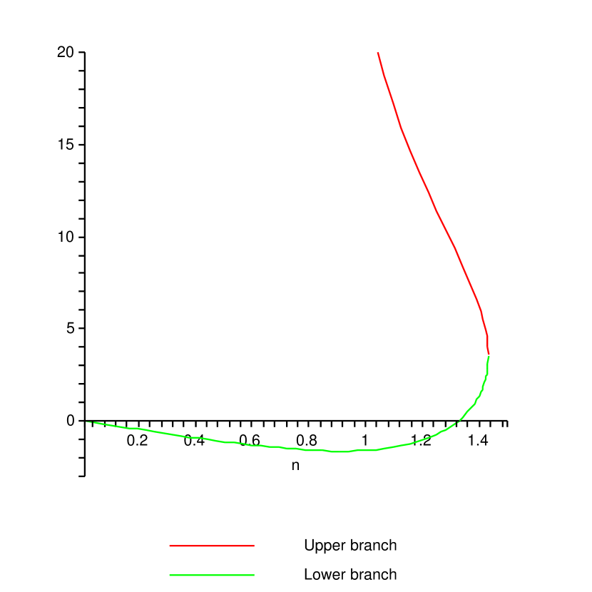
Figure 1: Plot of the upper ($r_{b}=r_{b+}$) and lower ( $r_{b}=r_{b-}$) TB masses (for $k=10$, $l=\sqrt{3}$).

In figure 1 we plot the masses of the upper branch ($r>r_{b+}$) and the lower branch ($r>r_{b-}$) solutions as a function of the nut parameter $n$. We can see that there is a range for the nut charge for which the mass of the lower branch solution becomes negative, while the mass of the upper branch solution is always positive.

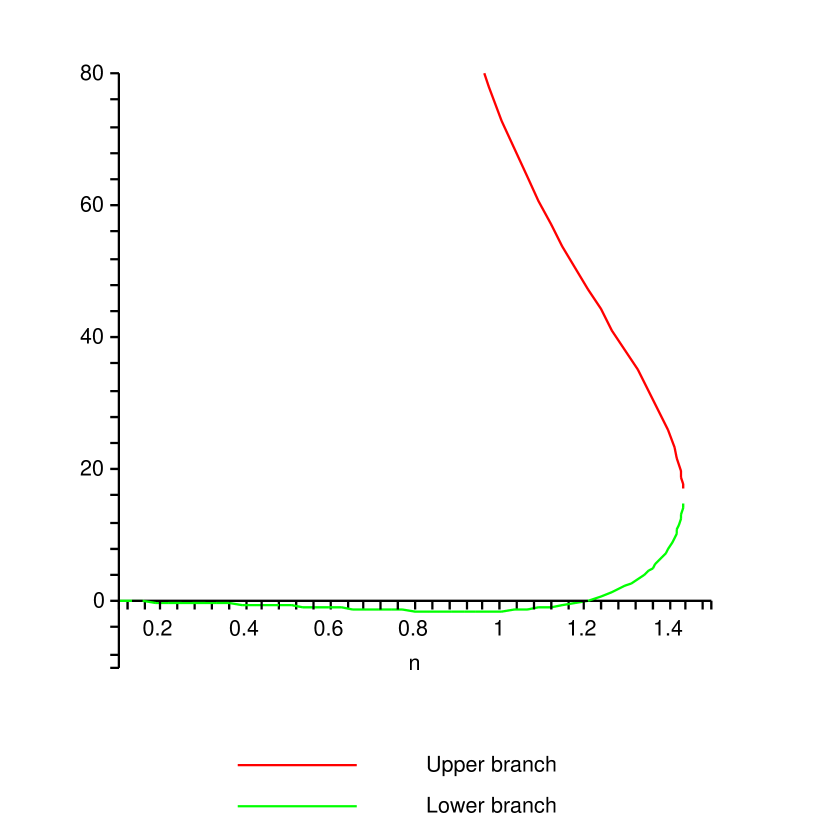
Figure 2: Plot of the upper ($r_{b}=r_{b+}$) and lower ( $r_{b}=r_{b-}$) TB entropies (for $k=10$, $l=\sqrt{3}$).

We plot the entropy as a function of the nut charge in figure 2, including the lower branch solutions. As is obvious from this figure, the entropy for the lower branch does become negative if $n<1.19355$. The entropy for the upper branch solutions is always positive.

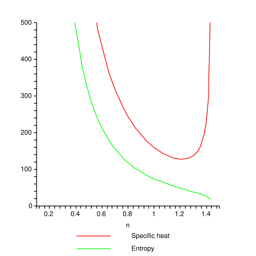
Figure 3: Plot of the upper branch bolt entropy and specific heat (for $k=10$, $l=\sqrt{3}$).

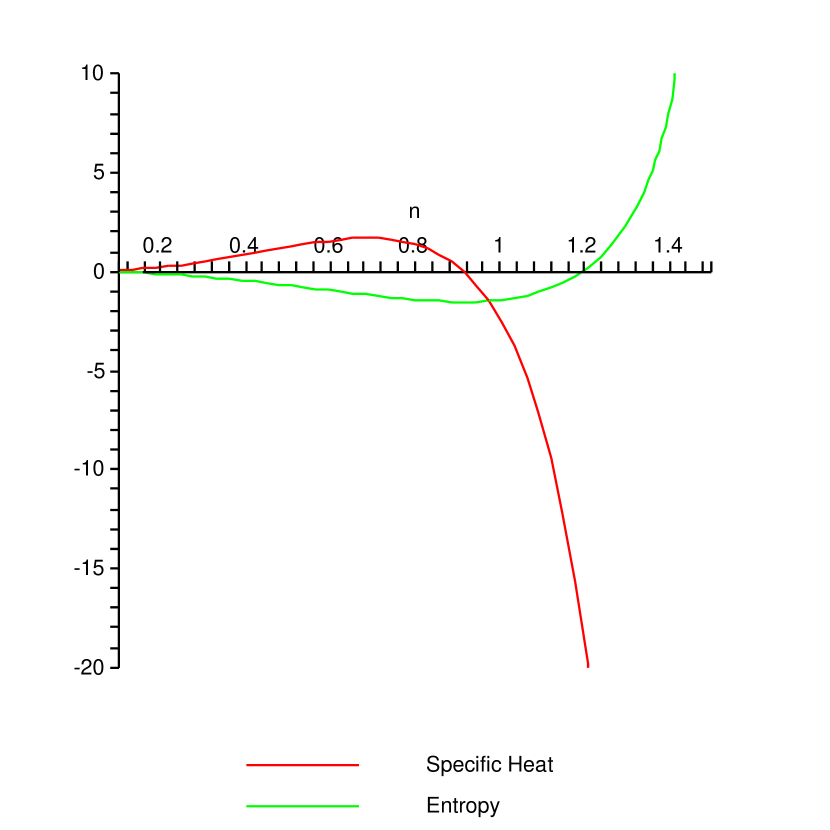
Figure 4: Plot of the lower branch bolt entropy and specific heat (for $k=10$, $l=\sqrt{3}$).

In figure 3 we plot the entropy and the specific heat versus the nut charge for the upper branch solutions. In this case the entropy and the specific heat are always positive. In figure 4 we plot the entropy and the specific heat as a function of the nut charge for the lower branch bolt solutions. We can see again that the entropy is negative if $n<1.19355$ while the specific heat is positive if $n<0.91338$ and negative otherwise, implying that the Lorentzian version of the lower branch solutions is thermally unstable. In both cases the specific heat diverges near $T=T_{min}$ (or $n=n_{max}$).

6.3 The Nut case

As we have seen above in the $\mathbb{C}$-approach, besides the usual Bolt solutions, one can also obtain the so-called Nut-solutions. For these solutions the fixed-point set of the Killing vector $\frac{\partial}{\partial T}$ is zero-dimensional. This can happen only if $\tau_{c}=N$ in the above equations, that is if $F(\tau_{c}=N)=0$ and also

$$\frac{4\pi}{|F^{\prime}(\tau_{c}=N)|}=\frac{8\pi N}{q}$$ (54)

are satisfied. Recall that $q=1$ for the Nut solution in the $\mathbb{C}$-approach.

However, since we are interested in the analytic continuations that could take the $\mathbb{C}$-results to the $\mathbb{R}$-results we shall slightly modify our ansatz using the lesson learned in dealing with the Bolt cases. Namely, instead of focussing on $\tau_{c}=N$ (which clearly becomes imaginary when we analytically continue $N\rightarrow in$) we shall look for a solution of the form $\tau_{c}=pN$ where $p$ is a positive real number. Then the usual Taub-Nut solution in the $\mathbb{C}$-approach corresponds to $p=1$, while other values of $p>1$ correspond to Bolt-type solutions.

The limit $p=1$ must be treated with special care since in the Nut solution $\tau_{c}=N$ is a double root of the numerator of $F(r)$, while in the Bolt case we assume that $\tau_{c}$ is a single root. The difference arises when computing the periodicity $\beta_{c}=\frac{4\pi}{|F^{\prime}(pN)|}$; accounting for the double root, it turns out that one should multiply by $2$ the result from the Bolt case in order to recover the correct periodicity of the Nut.

It is easy to check now that the above conditions will fix the periodicity of the coordinate $T$ to be $\beta_{c}=\frac{8\pi N}{q}$ where now $q$ is a complicated function of $p$, $l$ and $N$ while the value of the mass parameter is given by

$$m_{c} = \frac{N[(1+p^{2})l^{2}+(p^{4}-6p^{2}-3)N^{2}]}{2pl^{2}}$$ (55)

Using the counterterm method, for a bolt located at $r_{c}=pN$ we obtain:

$$I_{c} = \frac{\pi N^{2}[(p^{2}+1)l^{2}-(p^{4}+3)N^{2}]}{l^{2}+3N^{2}(p^{2}-1)}$$

$$S_{c} = \frac{\pi N^{2}[(p^{2}+1)l^{2}-3(p^{4}+3)N^{2}]}{l^{2}-3N^{2}(p^{2}-1)}$$ (56)

Notice that in the limit $p\rightarrow 1$ one recovers the previous expressions for the action and respectively the entropy of the Taub-Nut-AdS solution (38) up to the factor of $2$, as explained above.

Let us apply now our prescription from going from the $\mathbb{C}$-approach to the $\mathbb{R}$-approach. In this case we shall analytically continue $N\rightarrow in$ and also $q\rightarrow ik$ (which in the Nut case corresponds in fact to $p\rightarrow-ip$). Then the location of the nut becomes $\tau_{r}=pn$ in the $\mathbb{R}$-approach, yielding a real value for $\tau_{r}$, while the value of the mass parameter is also real

$$m_{r}=\frac{n[(p^{4}+6p^{2}-3)n^{2}-l^{2}(1-p^{2})]}{2pl^{2}}$$ (57)

Now the periodicity of the coordinate $t$ is given by $\frac{8\pi n}{|k|}$, with $k=(q)_{p=-ip}$. For $p=1$ we obtain:

$$k=2\left(\frac{6n^{2}}{l^{2}}+1\right)$$ (58)

while value of the mass parameter is $m_{r}=\frac{2n^{3}}{l^{2}}$, the action is

$$I_{r}=-\frac{4\pi n^{4}}{l^{2}+6n^{2}}$$ (59)

However, since the location of the ‘bolt’ $r=n$ is not of the form (48) unless we assume a relationship between $n$ and $l$ we conclude that the first law of thermodynamics is not satisfied for the Lorentzian Taub-Nut-AdS solution in the $\mathbb{R}$-approach.

6.4 The flat-space limit

Leaving the more detailed study of the thermodynamics of the above solutions for future work, let us now briefly discuss the case in which the cosmological constant vanishes. Notice that this condition corresponds to $l\rightarrow\infty$ and in this limit we recover the Taub-NUT solutions in a flat background. Special care must be taken when discussing the analytic continuation from the Euclidian sector to the Lorentzian one. Let us consider first the Lorentzian Taub-Nut-AdS solution. In the limit $l\rightarrow\infty$ we obtain the action $I_{r}=0$, the conserved mass is also zero in this limit. These results are in agreement with the expectation that the only way to have $r=n$ as a root of the Lorentzian function

$$F(r)=\frac{r^{2}-2mr-n^{2}}{r^{2}+n^{2}}$$

is to take $m=0$.

In the bolt case we obtain by analytic continuation $r_{r}=\frac{2n}{k}$ and the mass parameter is

$$m_{r}=n\frac{4-k^{2}}{4k}$$

while the action and the entropy are given by:

$$I_{r}=\pi n^{2}\frac{4-k^{2}}{k^{2}},~{}~{}~{}~{}~{}S_{r}=\pi n^{2}\frac{4-k^{2}}{k^{2}},~{}~{}~{}~{}~{}C_{r}=2\pi n^{2}\frac{k^{2}-4}{k^{2}}$$ (60)

As in the Euclidian sector we have $q=1$ (since if $q>1$ then $r_{b}$ is less than $n$) this will fix $k=1$ in the above relations. Further, note that although these expressions satisfy the first law of thermodynamics, the entropy and specific heat for the Lorentzian bolt in the flat spacetime have opposite signs, which means that the solution is thermally unstable. This is not unexpected if we recall that the Taub-NUT solutions in flat background correspond to the lower-branch Taub-NUT-AdS solutions, which are thermodynamically unstable.

7 Higher dimensional Taub-NUT-dS spaces

The above results can be easily extended to higher dimensional Taub-NUT spacetimes. For simplicity we shall focus only on the asymptotically de Sitter spacetimes.

First, let us notice the absence of higher dimensional Taub-Nut-dS solutions, which is a result analogous with that stating the absence of hyperbolic nuts in $AdS$-backgrounds [18, 33]. Quite generally we can see this by observing the behaviour of the function $F(\tau)$ near the root $\tau_{c}=N$. Since $F(\tau)$ takes negative values for points $\tau>\tau_{c}$ we deduce that there always exists a larger root of $F(\tau)$ that will contain the nut. Therefore, in our discussion we shall refer only to the higher-dimensional Bolt solutions. An analysis as the one performed in Section (6.1) assures us that the first law is satisfied in both approaches.

An analysis of the thermodynamics of the higher-dimensional Taub-NUT-dS spaces has been presented in [20]. It has been shown there that the thermodynamic behaviour of both the $\mathbb{R}$-approach and $\mathbb{C}$-approach quantities are qualitatively the same in $4s$-dimensions, a behaviour that is distinct from the common behaviour in $4s+2$ dimensions. This means that spaces of dimensionality $8,12,16,...$ have the same qualitative thermodynamic behaviour as the four-dimensional case, while spaces of dimensionality $10,14,18,...$ have the same behaviour as the six-dimensional case. We shall now illustrate equivalence of the two approaches in six-dimensions; the other $4s+2$ higher-dimensional cases are analogous.

The Taub-NUT-dS metric in six dimensions, constructed over an $S^{2}\times S^{2}$ base is given by:

$$ds^{2}=V(\tau)(dt+2n\cos\theta_{1}d\varphi_{1}+2n\cos\theta_{2}d\varphi_{2})^{2}-\frac{d\tau^{2}}{V(\tau)}+(\tau^{2}+n^{2})(d\Omega_{1}^{2}+d\Omega_{2}^{2})$$

where

$$V(\tau) = \frac{3\tau^{6}-(l^{2}-15n^{2})\tau^{4}-3n^{2}(2l^{2}-15n^{2})\tau^{2}+3n^{4}(l^{2}-5n^{2})+6ml^{2}\tau}{3(\tau^{2}+n^{2})^{2}l^{2}}$$

$$d\Omega_{i}^{2} = d\theta_{i}^{2}+\sin^{2}\theta_{i}d\varphi_{i}^{2}$$ (61)

Removal of the Misner string singularities in the metric forces us to take $12\pi|n|$ as the periodicity of the time coordinate. Similar with the $4$-dimensional case, we shall impose an extra periodicity $\frac{4\pi}{|V^{\prime}(\tau_{r})|}$. Matching the two values leads to the condition:

$$\beta_{r}=\frac{4\pi}{|V^{\prime}(\tau_{r})|}=\frac{12\pi|n|}{k}$$

where $V(\tau_{r})=0$ and $k$ is a positive integer. This fixes the bolt location to be given by the formula:

$$\tau_{r}=\frac{kl^{2}+\sqrt{k^{2}l^{4}-900n^{4}+180n^{2}l^{2}}}{30n}$$

and by requiring real values for $\tau_{r}$ we must restrict the allowed range of the nut charge to be:

$$|n|\leq l\frac{\sqrt{90+30\sqrt{k^{2}+9}}}{30}$$

In the $\mathbb{C}$-approach we make the analytic continuations $t\rightarrow iT$ and $n\rightarrow iN$. Then the function $V(\tau)$ is continued to $F(\tau)$ . Imposing the periodicity condition

$$\beta_{c}=\frac{4\pi}{|F^{\prime}(\tau_{c})|}=\frac{12\pi|N|}{q}$$

where $\tau_{c}$ is a root of $F(\tau)$ we find

$$\tau_{c}=\frac{ql^{2}+\sqrt{q^{2}l^{4}+900N^{4}+180N^{2}l^{2}}}{30N}$$

It is easy to see now that starting, for instance, with the $\mathbb{C}$-quantities and using the analytic continuations $N\rightarrow in$ and $q\rightarrow ik$ we recover the corresponding $\mathbb{R}$-quantities and vice-versa. This equivalence extends to all thermodynamic quantities computed using the counterterm approach.

8 Discussion

The work of this paper was motivated by the observation that the path-integral formalism can be extended to asymptotically de Sitter spacetimes to describe quantum correlations between timelike histories, providing a foundation for gravitational thermodynamics at past/future infinity [9]. The key result is the generalization (9) of the Gibbs-Duhem relation to asymptotically dS spacetimes.

In order to employ this relation it is necessary to analytically continue the spacetime near past/future infinity.  There are two apparently distinct ways of doing this – the $\mathbb{R}$-approach and the $\mathbb{C}$-approach. The $\mathbb{C}$-approach is closest to the more traditional method of obtaining Euclidian sections for asymptotically flat and AdS spacetime. The $\mathbb{R}$-approach refers to the Lorentzian section, and makes use of the path integral formalism only insofar as the generalized Gibbs-Duhem relation (9) is employed.

The main result of this paper is the demonstration that the $\mathbb{R}$ and $\mathbb{C}$-approaches are equivalent, in the sense that we can start from the $\mathbb{C}$-approach results and derive by consistent analytic continuations (i.e., using a well-defined prescription for performing the analytic continuations) all the results from the $\mathbb{R}$-approach. There are no a-priori obstacles in taking the opposite view, in which the $\mathbb{C}$-approach results are derived from the respective $\mathbb{R}$-approach results. However, one could still argue that the $\mathbb{C}$-approach is the more basic one, as in it the periodicity conditions appear more naturally than in the $\mathbb{R}$-approach.

On the other hand, the $\mathbb{R}$-approach, when used without the justification that comes from the $\mathbb{C}$-approach, raises some interesting questions. Even applied to simple cases such as the Schwarzschild-dS solution, one may take the view that in the absence of the nut charge one could still consider a periodicity on the time coordinate in the Lorentzian sector given by $\beta_{r}=8\pi m$. A more orthodox interpretation would be that $\beta_{r}$ in the Lorentzian sector is simply the inverse temperature (as related by the surface gravity of the black hole horizon) and is not related to a real periodicity of the time coordinate. Whether or not this is indeed a necessary condition remains to be seen.

Using this equivalence we then proposed an interpretation of the thermodyamic behaviour of nut-charged spacetimes. In the asymptotically dS case, we showed that while a subset of the Bolt solutions can have a sensible physical interpretation, the same does not hold for the Taub-Nut-dS solutions. Indeed, in the putative Taub-Nut-dS solution the nut is always enclosed in a larger cosmological ‘bolt’ and moreover it does not have a Lorentzian counterpart (i.e. it has no equivalent solution in the $\mathbb{R}$-approach). From these facts we conclude that there are no Taub-Nut-dS solutions. This situation holds despite the fact that a naive application of (9) to this case yields thermodynamic quantities that respect the first law of thermodynamics. Rather these quantities are the analytic continuations of their AdS counterparts under $l\rightarrow il$. Similar remarks apply to the lower-branch dS bolt cases. We have also found that this situation holds in higher dimensions: there are no Taub-Nut-dS solutions, in analogy with the non-existence of the hyperbolic nuts in AdS backgrounds [29].

Moreover, the $\mathbb{C}$-approach has been previously applied with success to more general cases - it has been proven to be very useful when treating for instance asymptotically AdS or flat Taub-NUT spaces. In particular, we have shown here that starting from the well-known results regarding the thermodynamics of the Nut and Bolt solutions in the Euclidian Taub-NUT-AdS case (which corresponds to our $\mathbb{C}$-approach) we can consistently make analytic continuations back to the Lorentzian sections, yielding a physical interpretation of the thermodynamics of such spacetimes. However, this holds only for the bolt solutions; we found that the Lorentzian AdS-Nut solution did not respect the first law of thermodynamics, rendering the physical interpretation of the Nut solution dubious at best.

We close by commenting on recent results concerning these spacetimes. It has been shown that there exist broad ranges of parameter space for which nut-charged spacetimes violate both the maximal mass conjecture and the N-bound, in both four dimensions and in higher dimensions. However it was subsequently argued [32] that even if the Taub-NUT-dS spaces do violate the maximal mass conjecture they also suffer of causal pathologies. However, this is not necessarily the case. As noted above in both the $\mathbb{R}$ and $\mathbb{C}$-approaches the maximal mass conjecture can be violated by choosing the parameter $m<0$, independent of whether or not the metric function has any roots [9, 28]. A detailed discussion of this situation has appeared recently [11], where it was emphasized that globally hyperbolic asymptotically dS spacetimes exist that violate the maximal mass conjecture. In the present context this will take place whenever the parameters $m$ and $N$ are such that the function (12) has no roots [20].

If horizons are present, the maximal mass conjecture and N-bound can both be violated and we have shown that this holds consistently for both approaches. Although these cases have regions containing closed timelike curves (CTC’s), our computations pertain to regions where CTCs are absent, namely outside the cosmological horizon. However, one could argue that such spacetimes are causally unstable. Whether any spacetimes containing horizons exist that violate one or both conjectures and that satisfy rigid constraints of causal stability remains an open question.

In AdS backgrounds it would be interesting to understand how the AdS-CFT correspondence works in this case, since the Lorentzian section of the Taub-NUT spaces contains closed timelike curves and so it is causally pathological. In fact it was recently noted [30, 33, 34, 35] that the boundary metric for the four-dimensional Lorentzian Taub-NUT-AdS spacetime is in fact the three-dimensional Gödel metric. This metric also has a bad reputation as being causally ill-behaved since for generic values of the parameters, the Gödel spacetime admits $CTC$’s through every point. The meaning of a quantum field theory in this background is still an open problem.

Recently the authors of [8] used successfully the $\mathbb{R}$-approach methods to study the Kerr-dS space-times. As the metric is stationary in this case and the continuation to the complex section involves the analytical continuation of the rotation parameter $a\rightarrow ia$, it would be interesting to see if there is a similar prescription for the analytical continuation of the results from the $\mathbb{R}$-approach and the $\mathbb{C}$-approach and vice-versa. Other interesting extensions of the present work could involve the study of the electric and magnetic charged versions of the Taub-NUT solutions (with or without rotation). A new set of nut-charged solutions in Einstein-Maxwell theory has been presented recently in [36, 37] and it would be interesting to see how one could extend our analysis to these spaces.

Acknowledgements

CS would like to thank Brenda Chng, Tomasz Konopka and Dumitru Astefanesei for valuable discussions during the completion of this work. This work was supported in part by the Natural Sciences & Engineering Research Council of Canada.

References

- [1] A. Strominger, “The dS/CFT correspondence,” JHEP 0110, 034 (2001) [arXiv:hep-th/0106113].
- [2] V. Balasubramanian, J. de Boer and D. Minic, “Holography, time and quantum mechanics,” [arXiv:gr-qc/0211003].
- [3] R. Bousso, JHEP 9907, 004 (1999); JHEP 0011, 038 (2000).
- [4] R. Bousso, O. DeWolfe and R. C. Myers, “Unbounded entropy in spacetimes with positive cosmological constant,” Found. Phys. 33, 297 (2003) [arXiv:hep-th/0205080].
- [5] A.M. Ghezelbash and R.B. Mann, JHEP 0201, 005 (2002).
- [6] R.G. Cai, Y.S. Myung and Y.Z. Zhang Phys. Rev. D65, 084019 (2002).
- [7] D. Astefanesei, R. Mann and E. Radu, “Reissner-Nordstroem-de Sitter black hole, planar coordinates and dS/CFT,” JHEP 0401, 029 (2004) [arXiv:hep-th/0310273].
- [8] A. M. Ghezelbash and R. B. Mann, “Entropy and mass bounds of Kerr-de Sitter spacetimes,” arXiv:hep-th/0412300.
- [9] R. Clarkson, A. M. Ghezelbash and R. B. Mann, “Entropic N-bound and maximal mass conjectures violation in four dimensional Taub-Bolt(NUT)-dS spacetimes,” Nucl. Phys. B 674, 329 (2003) [arXiv:hep-th/0307059].
- [10] R. Clarkson, A. M. Ghezelbash and R. B. Mann, “Mass, Action And Entropy Of Taub-Bolt-Ds Spacetimes,” Phys. Rev. Lett. 91, 061301 (2003) [arXiv:hep-th/0304097].
- [11] M. T. Anderson,“Existence and stability of even dimensional asymptotically de Sitter spaces,” [arXiv:gr-qc/0408072].
- [12] G.W. Gibbons and S.W. Hawking, Phys. Rev. D 15, 2752 (1977); J.D. Brown and J.W. York, Phys. Rev. D 47, 1407 (1993); J.D. Brown, J. Creighton and R.B. Mann, Phys. Rev. D 50, 6394 (1994); J. Creighton and R.B. Mann, Phys.Rev.D 52 (1995) 4569.
- [13] J.D. Brown, E. A. Martinez and J.W. York, Phys. Rev. Lett. 66 (1991) 2281; I.S. Booth and R.B. Mann Phys. Rev. Lett. 81 (1998) 5052.
- [14] C. W. Misner, J. Math. Phys. 4 (1963) 924; C. W. Misner, in Relativity Theory and Astrophysics I: Relativity and Cosmology, edited by J. Ehlers, Lectures in Applied Mathematics, vol. 8 (American Mathematical Society, Providence, RI, 1967), p. 160.
- [15] D. N. Page “Taub-NUT instanton with a Horizon” Phys. Lett. B 78 (1978) 249-251.
- [16] R. B. Mann, “Misner string entropy,” Phys. Rev. D 60, 104047 (1999) [arXiv:hep-th/9903229].
- [17] S. W. Hawking, C. J. Hunter and D. N. Page “Nut Charge, Anti-de Sitter Space and Entropy” Phys. Rev. D 59 (1999) 044033 [hep-th/9809035].
- [18] A. Chamblin, R. Emparan, C. V. Johnson and R. C. Myers, “Large N phases, gravitational instantons and the NUTs and bolts of AdS holography,” Phys. Rev. D 59, 064010 (1999) [arXiv:hep-th/9808177].
- [19] C. V. Johnson and H. G. Svendsen, “An exact string theory model of closed time-like curves and cosmological singularities,” Phys. Rev. D 70, 126011 (2004) [arXiv:hep-th/0405141].
- [20] R. Clarkson, A. M. Ghezelbash and R. B. Mann “A Review of the N-bound and the Maximal Mass Conjectures Using NUT-Charged dS Spacetimes” Int.J.Mod.Phys. A19 (2004) 3987-4036 [arXiv:hep-th/0408058].
- [21] V. Balasubramanian and P. Kraus, Commun. Math. Phys. 208, 413 (1999).
- [22] M. Henningson and K. Skenderis, JHEP 9807, 023 (1998); S.Y. Hyun, W.T. Kim and J. Lee, Phys. Rev. D59, 084020 (1999).
- [23] R. Mann and C. Stelea, “Nuttier (A)dS black holes in higher dimensions,” Class. Quantum. Grav. 21 1-25 (2004), [arXiv:hep-th/0312285].
- [24] H. Lu, D. N. Page and C. N. Pope, “New inhomogeneous Einstein metrics on sphere bundles over Einstein-Kaehler manifolds,” [arXiv:hep-th/0403079].
- [25] R. B. Mann and C. Stelea, “New Multiply Nutty Spacetimes,” [arXiv:hep-th/0508203].
- [26] D.A. Konkowski, T.M. Helliwell and L.C. Shepley, Phys. Rev. D31, 1178 (1985); D.A. Konkowski and T.M. Helliwell, Phys. Rev. D31, 1195 (1985).
- [27] L. G. Jensen, J. Louko and P. J. Ruback, “Biaxial Bianchi Type Ix Quantum Cosmology,” Nucl. Phys. B 351, 662 (1991).
- [28] R. Clarkson, L. Fatibene and R. B. Mann, “Thermodynamics of (d+1)-dimensional NUT-charged AdS spacetimes,” Nucl. Phys. B 652, 348 (2003) [arXiv:hep-th/0210280].
- [29] R. Emparan, C. V. Johnson and R. C. Myers, “Surface terms as counterterms in the AdS/CFT correspondence,” Phys. Rev. D 60, 104001 (1999) [arXiv:hep-th/9903238].
- [30] D. Astefanesei, R. B. Mann and E. Radu, “Breakdown of the entropy / area relationship for NUT-charged spacetimes,” [arXiv:hep-th/0406050].
- [31] P. Hoxha, R. R. Martinez-Acosta and C. N. Pope, “Kaluza-Klein consistency, Killing vectors, and Kaehler spaces,” Class. Quant. Grav. 17, 4207 (2000) [arXiv:hep-th/0005172].
- [32] V. Balasubramanian, “Accelerating universes and string theory,” Class. Quant. Grav. 21, S1337 (2004) [arXiv:hep-th/0404075].
- [33] D. Astefanesei, R. B. Mann and E. Radu, “Nut charged space-times and closed timelike curves on the boundary,” [arXiv:hep-th/0407110].
- [34] D. Astefanesei and E. Radu “Quantum effects in a rotating spacetime”, Int. J. Mod. Phys. D 11 715 (2002), [arXiv:gr-qc/0112029].
- [35] E. Radu “Gravitating non-abelian solutions with NUT charge” Phys. Rev. D 67 084030 (2003) [arXiv:hep-th/0211120].
- [36] R. B. Mann and C. Stelea, “New Taub-NUT-Reissner-Nordstroem spaces in higher dimensions,” [arXiv:hep-th/0508186].
- [37] A. M. Awad, “Higher dimensional Taub-NUTs and Taub-bolts in Einstein-Maxwell gravity,” [arXiv:hep-th/0508235].