Variational solution of the Yang-Mills Schrödinger equation in Coulomb gauge

Abstract

The Yang-Mills Schrödinger equation is solved in Coulomb gauge for the vacuum by the variational principle using an ansatz for the wave functional, which is strongly peaked at the Gribov horizon. A coupled set of Schwinger-Dyson equations for the gluon and ghost propagators in the Yang-Mills vacuum as well as for the curvature of gauge orbit space is derived and solved in one-loop approximation. We find an infrared suppressed gluon propagator, an infrared singular ghost propagator and a almost linearly rising confinement potential.

I Introduction

To understand the low energy sector of QCD is one of the most challenging problems in quantum field theory. Nowadays, quantum field theory and, in particular, QCD is usually studied within the functional integral approach. This approach is advantagous for a perturbative calculation, where it leads automatically to a Feynman diagrammatic expansion. Within this approach asymptotic freedom of QCD was shown R1 , which manisfests itself in deep inelastic scattering experiments. In addition, the functional integral approach is the basis for numerical lattice calculations R2 , the only rigorous non-perturbative approach available at the moment. These lattice methods have provided considerable insights into the nature of the Yang-Mills vacuum. Lattice investigations performed over the last decade, have accumulated evidence for two confinement scenarios: the dual Meissner effect based on a condensate of magnetic monopoles R3 and the vortex condensation picture R4 (For a recent review see ref. R5 ). In both cases the Yang-Mills functional integral is dominated in the infrared sector by topological field configurations (magnetic monopoles RX1 or center vortices RX2 ), which seem to account for the string tension, i.e. for the confining force. Yet another confinement mechanism was proposed by Gribov R22 , further elaborated by Zwanziger R23 and tested in lattice calculations R24 . This mechanism is based on the infrared dominance of the field configurations near the Gribov horizon in Coulomb gauge. This mechanism of confinement is compatible with the center vortex and magnetic pictures, given the fact, that lattice center vortex and magnetic monopole configurations lie on the Gribov horizon R26 .
Despite the great successes of lattice calculations in the exploration of strong interaction physics R6 , a complete understanding of the Yang-Mills theory will probably not be provided by the lattice simulations alone, but requires also analytical tools. Despite of its success in quantum field theory, in particular in perturbation theory and its appeal in semi-classical and topological considerations R9 , the path integral approach may not be the most economic method for analytic studies of non-perturbative physics. As an example consider the hydrogen atom. Calculating its electron spectrum exactly in the path integral approach is exceedingly complicated R7 , while the exact spectrum can be obtained easily by solving the Schrödinger equation. One might therefore wonder, whether the Schrödinger equation is also the appropriate tool to study the low-energy sector of Yang-Mills theory, and in particular of QCD.
The Yang-Mills Schrödinger equation is based on the canonical quantization in Weyl gauge $A_{0}=0$ R8 , where Gauß’ law has to be enforced as a constraint to the wave functional to guarantee gauge invariance. The implementation of Gauß’ law is crucial. This is because any violation of Gauß’ law generates spurious color charges during the time evolution. These spurious color charges can screen the actual color charges and thereby spoil confinement . Several approaches have been advocated to explicitly resolve Gauß’ law by changing variables resulting in a description in terms of a reduced number of unconstrained variables. This can be accomplished either by choosing a priori gauge invariant variables R10 or by fixing the gauge, for example, to unitary gauge R11 , to Coulomb gauge R12 or to a modified version of axial gauge R13 . In particular, the Yang-Mills Hamiltonian resulting after eliminating the gauge degrees of freedom in Coulomb gauge, was derived in ref. R12 . Alternatively, one has attempted to project the Yang-Mills wave functional onto gauge invariant states (which a priori fulfill Gauß’ law) R14 . The equivalence between gauge fixing and projection onto gauge invariant states can be seen by noticing that the Faddeev-Popov determinant provides the Haar measure of the gauge group R15 .
In this paper we will variationally solve the stationary Yang-Mills Schrödinger equation in Coulomb gauge for the vacuum. Such a variational approach was previously studied in refs. R16 , R17 , where a Gaussian ansatz for the Yang-Mills wave functional was used. Our approach is conceptually simular to, but differs essentially from refs. R16 ; R17 in two respects: i) we use a different ansatz for the trial wave functional and ii) we include fully the curvature of the space of gauge orbits induced by the Faddeev-Popov determinant. We use a vacuum wave functional, which is strongly peaked at the Gribov horizon. Such a wave functional is motivated by the results of ref. R19 and by the fact, that the dominant infrared degrees of freedom like center vortices lie on the Gribov horizon R26 . The Faddeev-Popov determinant was completely ignored in ref. R16 and only partly included in ref. R17 . (In addition, ref. R17 uses the angular approximation). We will find however, that a full inclusion of the curvature induced by the Faddeev-Popov determinant is absolutely crucial and vital for the infrared regime and, in particular, for the confinement property of the Yang-Mills theory. The organization of the paper is as follows:

In section II we briefly review the hamiltonian formulation of Yang-Mills theory in Coulomb gauge and fix our notation. In section III we present our vacuum wave functional and calculate the relevant expectation values. The vacuum energy functional is calculated and minimized in section IV resulting in a set of coupled Schwinger-Dyson equations for the gluon energy, the ghost and Coulomb form factors and the curvature in gauge orbit space. The asymptotic behaviours of these quantities in both the ultraviolet and infrared regimes are investigated in section V. Section VI is devoted to the renormalization of the Schwinger-Dyson equations. The numerical solutions to the renormalized Schwinger-Dyson equations are presented in section VII. Finally in section VIII we present our results for the static Coulomb potential. Our conclusions are given in section IX. A short summary of our results has been previously reported in ref. R9a .

II Hamiltonian formulation of Yang-Mills theory in Coulomb gauge

The canonical quantization of gauge theory is usually performed in the Weyl gauge $A_{0}=0$. In this gauge the spatial components of the gauge field ${\bf{A}}({\bf x})$ are the “cartesian” coordinates and the corresponding canonically conjugated momenta

$$\Pi^{a}_{k}({\bf x})=\frac{\delta}{i\delta A^{a}_{k}({\bf x})}\hskip 2.84544pt,$$ (1)

defined by the equal time commutation relation

$$\left[A^{a}_{k}({{\bf x}}),\Pi^{b}_{l}({\bf y})\right]=i\delta^{ab}\delta_{kl}\delta\left({\bf x}-{\bf y}\right)$$ (2)

represent the color electric field. The Yang-Mills Hamiltonian is then given by

$$H=\frac{1}{2}\int d^{3}x\left[\Pi^{a}_{k}({\bf x})^{2}+B^{a}_{k}({\bf x})^{2}\right]\hskip 2.84544pt,$$ (3)

where

$$B_{k}=\frac{1}{2}\epsilon_{kij}F_{ij}\hskip 2.84544pt,\hskip 2.84544ptgF_{ij}=\left[D_{i},D_{j}\right]\hskip 2.84544pt,\hskip 2.84544ptD_{i}=\partial_{i}+gA_{i}$$ (4)

is the colormagnetic field with $F_{ij}$ being the non-Abelian field strength and $D_{i}$ the covariant derivative. We use anti-hermitian generators $T^{a}$ of the gauge group with normalization $tr(T^{a}T^{b})=-\frac{1}{2}\delta^{ab}$ $(A=A^{a}T^{a})$.
The Hamiltonian (3) is invariant under spatial gauge transformations $U({\bf x})$

$$A\to A^{U}=UAU^{\dagger}+\frac{1}{g}U\partial U^{\dagger}\hskip 2.84544pt.$$ (5)

Accordingly the Yang-Mills wave functional $\Psi[A]=\langle A|\Psi\rangle$ can change only by a phase, which is given by

$$\Psi[A^{U}]=e^{i\Theta n[U]}\Psi[A]\hskip 2.84544pt,$$ (6)

where $\Theta$ is the vacuum angle and $n[U]$ denotes the winding number of the mapping $U({\bf x})$ from the 3-dimensional space ${\mathbb{R}}^{3}$ (compactified to $S_{3}$) into the gauge group. In this paper we will not be concerned with topological aspects of gauge theory and confine ourselves to “small” gauge transformations with $n[U]=0$.
Invariance of the wave functional under “small” gauge transformations is guaranteed by Gauß’ law

$$\hat{D}_{k}(A)\Pi_{k}\Psi[A]=\rho_{m}\hskip 2.84544pt,$$ (7)

where $\rho_{m}$ is the color density of the matter (quark) field and $\hat{D}_{i}(A)$ denotes the covariant derivative in the adjoint representation of the gauge group

$$\hat{D}_{i}(A)=\partial_{i}+g\hat{A}_{i}\hskip 2.84544pt,\hskip 2.84544pt\hat{A}_{i}=A^{a}_{i}\hat{T}^{a}\hskip 2.84544pt,\hskip 2.84544pt(\hat{T}^{a})^{bc}=f^{bac}$$ (8)

with $f^{abc}$ being the structure constant of the gauge group. Throughout the paper we use a hat “^” to denote quantities defined in the adjoint representation of the gauge group. The Gauß’ law constraint (7) on the Yang-Mills wave functional can be resolved by fixing the residual gauge invariance, eq. (5). This eliminates the unphysical gauge degrees of freedom and amounts to a change of coordinates from the “cartesian” coordinates to curvilinear ones, which introduces a non-trivial Jacobian (Faddeev-Popov determinant) ${\cal{J}}[A]$. In this paper we shall use the Coulomb gauge

$$\partial_{k}A_{k}({\bf x})=0\hskip 2.84544pt.$$ (9)

In this gauge the physical degrees of freedom are the transversal components of the gauge fields

$$A^{\perp}_{i}({{\bf x}})=t_{ij}({{\bf x}})A_{j}({{\bf x}})\hskip 2.84544pt,$$ (10)

where

$$t_{ij}({\bf x})=\delta_{ij}-\frac{\partial_{i}\partial_{j}}{\partial^{2}}$$ (11)

is the transversal projector. The corresponding canonical momentum is given by

$$\Pi^{\perp a}_{i}({\bf x})=t_{ik}({\bf x})\frac{\delta}{i\delta A^{a}_{k}({\bf x})}:=\frac{\delta}{i\delta A^{\perp a}_{i}({\bf x})}$$ (12)

and satisfies the equal-time commutation relation

$$\left[A^{\perp a}_{i}({\bf x})\hskip 2.84544pt,\hskip 2.84544pt\Pi^{\perp b}_{j}({\bf x}^{\prime})\right]=i\delta^{ab}t_{ij}({\bf x})\delta\left({{\bf x}-{\bf x}^{\prime}}\right)\hskip 2.84544pt$$ (13)

In Coulomb gauge (9) the Yang-Mills Hamiltonian is given by R12

$$H = \frac{1}{2}\int d^{3}x\left[{\cal{J}}^{-1}[A^{\perp}]\Pi^{a}_{i}({\bf x}){\cal{J}}[A^{\perp}]\Pi^{a}_{i}({\bf x})+B^{a}_{i}({{\bf x}})^{2}\right]$$ (14)

$$+\frac{g^{2}}{2}\int d^{3}x\int d^{3}x^{\prime}{\cal{J}}^{-1}[A^{\perp}]\rho^{a}({\bf x})F^{ab}\left({{\bf x}},{{\bf x}^{\prime}}\right){\cal{J}}[A^{\perp}]\rho^{b}({{\bf x}^{\prime}})\hskip 2.84544pt.$$

where

$${\cal{J}}[A^{\perp}]=Det\left(-\partial_{i}\hat{D}_{i}\right)\hskip 2.84544pt$$ (15)

is the Faddeev-Popov determinant with $\hat{D_{k}}\equiv\hat{D_{k}}(A^{\perp})$ .

The kinetic part of the hamiltonian (first term) is reminiscent to the functional version of the Laplace-Beltrami operator in curvilinear space. The magnetic energy (second term) represents the potential for the gauge field. Finally, the last term arises by expressing the kinetic part of eq. (3) in terms of the transversal gauge potentials (curvilinear coordinates) satisfying the Coulomb gauge, i.e. by resolving Gauß’ law R12 . This term describes the interaction of static non-Abelian color (electric) charges with density

$$\rho^{a}({{\bf x}})=-\hat{A}^{\perp ab}_{i}({{\bf x}})\Pi^{b}_{i}({{\bf x}})+\rho^{a}_{m}({\bf x})$$ (16)

through the Coulomb propagator

$$F^{ab}\left({{\bf x},{\bf x}^{\prime}}\right)=\langle{{\bf x}}a|\left(-\hat{D}_{i}\partial_{i}\right)^{-1}(-\partial^{2})\left(-\hat{D}_{j}\partial_{j}\right)^{-1}|{{\bf x}^{\prime}}b\rangle\hskip 2.84544pt\hskip 2.84544pt$$ (17)

which is the non-Abelian counter part of the usual Coulomb propagator $\langle{{\bf x}}|\frac{1}{-\partial^{2}}|{{\bf x}^{\prime}}\rangle$ in QED and reduces to the latter for the perturbative vacuum $A^{\perp}=0$. If not stated otherwise, in the following we will assume $\rho_{m}=0$.

Since the Hamiltonian (14) does not change when ${\cal{J}}[A^{\perp}]$ is multiplied by a constant we can rescale the Jacobian ${\cal{J}}$ by the irrelevant constant $Det\left(-\partial^{2}\right)$

$${\cal{J}}[A^{\perp}]=\frac{Det\left(-\hat{D}_{i}\partial_{i}\right)}{Det\left(-{\partial^{2}}\right)}$$ (18)

such that ${\cal{J}}[A^{\perp}=0]=1$.
The Faddeev-Popov matrix $\left(-\hat{D}_{i}\partial_{i}\right)$ represents the metric tensor in the color space of gauge connections satisfying the Coulomb gauge. Accordingly its determinant enters the measure of the integration over the space of transversal gauge connections and the matrix element of an observable $O[A^{\perp},\Pi]$ between wave functionals $\Psi_{1}[A^{\perp}],\Psi_{2}[A^{\perp}]$ is defined by

$$\langle\Psi_{1}|O|\Psi_{2}\rangle=\int{\cal D}A^{\perp}{\cal{J}}[A^{\perp}]\Psi^{*}_{1}[A^{\perp}]O[A^{\perp},\Pi]\Psi_{2}[A^{\perp}]\hskip 2.84544pt.$$ (19)

Here, the integration is over transversal gauge potentials $A^{\perp}$ only. The same expression (19) is obtained by starting from the matrix element in Weyl gauge (with gauge invariant wave functionals) and implementing the Coulomb gauge by means of the Faddeev-Popov method.

Like in the treatment of spherically symmetric systems in quantum mechanics it is convenient to introduce “radial” wave functions by

$$\tilde{\Psi}[A^{\perp}]={\cal{J}}^{\frac{1}{2}}[A^{\perp}]\Psi[A^{\perp}]$$ (20)

and transform accordingly the observables

$$\tilde{O}={\cal{J}}^{\frac{1}{2}}[A^{\perp}]O{\cal{J}}^{-\frac{1}{2}}[A^{\perp}]\hskip 2.84544pt.$$ (21)

Formally, the Jacobian then disappears from the matrix element

$$\langle\Psi_{1}|O|\Psi_{2}\rangle=\int DA^{\perp}\tilde{\Psi}_{1}^{*}[A^{\perp}]\hskip 2.84544pt\tilde{O}\hskip 2.84544pt\tilde{\Psi}_{2}[A^{\perp}]:=\langle\tilde{\Psi}_{1}|\tilde{O}|\tilde{\Psi}_{2}\rangle\hskip 2.84544pt.\hskip 2.84544pt\hskip 2.84544pt$$ (22)

In the present paper we are interested in the vacuum structure of Yang-Mills theory. The vacuum wave functional, defined as solution to the Yang-Mills Schrödinger equation

$$H\Psi=E\Psi$$ (23)

for the lowest energy eigenstate, can be obtained from the variational principle

$$\frac{\langle\Psi|H|\Psi\rangle}{\langle\Psi|\Psi\rangle}\longrightarrow\mbox{min}\hskip 2.84544pt.$$ (24)

To work out the expectation value of the Hamiltonian $\tilde{H}={\cal{J}}^{\frac{1}{2}}H{\cal{J}}^{-\frac{1}{2}}$ it is convenient to perform a partial (functional) integration in the kinetic and Coulomb terms. Assuming as usual that the emerging surface terms vanish, one finds

$$\langle\Psi|H|\Psi\rangle=\langle\tilde{\Psi}|\tilde{H}|\tilde{\Psi}\rangle=E_{k}+E_{p}+E_{c}\hskip 2.84544pt,$$ (25)

where

$$E_{k} =\frac{1}{2}\int{\cal D}A^{\perp}\int d^{3}x\left[\tilde{\Pi}^{a}_{i}({\bf x})\tilde{\Psi}[A^{\perp}]\right]^{*}\left[\tilde{\Pi}^{a}_{i}({\bf x})\tilde{\Psi}[A^{\perp}]\right]$$ (26)

$$E_{p} =\frac{1}{2}\int{\cal D}A^{\perp}\int d^{3}x\hskip 2.84544pt\tilde{\Psi}^{*}[A^{\perp}]B^{a}_{i}({\bf x})^{2}\tilde{\Psi}[A^{\perp}]$$ (27)

$$E_{c} =-\frac{g^{2}}{2}\int{\cal D}A^{\perp}\int d^{3}x\int d^{3}x^{\prime}\left[\tilde{\Pi}^{c}_{i}({\bf x})\tilde{\Psi}[A^{\perp}]\right]^{*}\hat{A}^{\perp ca}_{i}({\bf x})F^{ab}({\bf x},{\bf x}^{\prime})\hat{A}^{\perp bd}_{j}({\bf x}^{\prime})\left[\tilde{\Pi}^{d}_{j}({\bf x}^{\prime})\tilde{\Psi}[A^{\perp}]\right]\hskip 2.84544pt,$$ (28)

where $\tilde{\Pi}$ is defined below in eq. (II). Note, integration is over the transversal part $A^{\perp}$ only. In order to prevent the equations from getting cluttered we will in the following often write $A$ instead of $A^{\perp}$, and $\Pi$ instead of $\Pi^{\perp}$, but it will be always clear from the context, when the transversal part is meant.

The transformed momentum operator $\tilde{\Pi}^{a}_{i}(x)$ is explicitly given by

$$\tilde{\Pi}^{a}_{k}({\bf x}) ={\cal{J}}^{\frac{1}{2}}[A^{\perp}]\Pi^{\perp a}_{k}({\bf x}){\cal{J}}^{-\frac{1}{2}}[A^{\perp}]$$

$$=\Pi^{\perp a}_{k}({\bf x})-\frac{1}{2}\Pi^{\perp a}_{k}({\bf x})\ln{\cal{J}}[A^{\perp}]$$

$$=\Pi^{\perp a}_{k}({\bf x})+\frac{g}{2i}t_{kl}({\bf x})\hskip 2.84544pttr\left[\hat{T}^{a}\left(\partial^{{\bf y}}_{l}G({\bf y},{\bf x})\right)_{{\bf y}={\bf x}}\right]\hskip 2.84544pt,$$ (29)

where we have introduced the inverse of the Faddeev-Popov operator

$$G=\left(-\hat{D}_{i}\partial_{i}\right)^{-1}\hskip 2.84544pt,$$ (30)

which is a matrix in color and coordinate space

$$\langle{\bf x}a|G|{\bf x}^{\prime}b\rangle=\langle{\bf x}a|\left(-\hat{D}_{i}\partial_{i}\right)^{-1}|{\bf x}^{\prime}b\rangle:=G^{ab}\left({\bf x},{\bf x}^{\prime}\right)\hskip 2.84544pt.$$

Its vacuum expectation value (to be defined below) represents the ghost propagator. Expanding this quantity in terms of the gauge field, we obtain

$$G=\left(-{\partial^{2}}-g\hat{A}_{i}\partial_{i}\right)^{-1}=G_{0}\sum\limits^{\infty}_{n=0}\left(g\hat{A}_{i}\partial_{i}G_{0}\right)^{n}\hskip 2.84544pt,$$ (31)

where

$$G_{0}\left({\bf x},{\bf x}^{\prime}\right)=\langle{\bf x}|\left(-{\partial^{2}}\right)^{-1}|{\bf x}^{\prime}\rangle=\frac{1}{4\pi|{\bf x}-{\bf x}^{\prime}|}$$ (32)

is the free ghost propagator, which is nothing but the ordinary static Coulomb propagator in QED.
From the expansion, eq. (31), it is seen, that the ghost propagator satisfies the identity

$$G=G_{0}+G_{0}g\hat{A}_{i}\partial_{i}G\hskip 2.84544pt,$$ (33)

where we have used the usual short hand matrix notation in functional and color space.

III The vacuum wave functional and propagators

So far all our considerations have been exact, i.e. no approximation has been introduced. To proceed further, we have to specify the (vacuum) wave functional $\tilde{\Psi}[A]$.

III.1 The vacuum wave functional

Inspired by the known exact wave functional of QED in Coulomb gauge R18 , we will consider a Gaussian ansatz in the transversal gauge fields

$$\tilde{\Psi}[A]=\langle A|\omega\rangle={\cal N}\exp\left[-\frac{1}{2}\int d^{3}x\int d^{3}x^{\prime}A^{\perp a}_{i}({\bf x})\omega({\bf x},{\bf x}^{\prime})A^{\perp a}_{i}({\bf x}^{\prime})\right]\hskip 2.84544pt,$$ (34)

where ${\cal N}$ is a normalization constant chosen so that $\langle\tilde{\Psi}|\tilde{\Psi}\rangle=1$. By translational and rotational invariance the integral kernel in the exponent of the Gaussian wave functional $\omega({\bf x},{\bf x}^{\prime})$ can depend only on $|{\bf x}-{\bf x}^{\prime}|$. For simplicity we have chosen the integral kernel $\omega({\bf x},{\bf x}^{\prime})$ to be a color and Lorentz scalar. This is justified by isotropy of color and Lorentz space.
Of course, such a Gaussian ansatz is ad hoc at this stage and can be justified only a posteriori. Let us also stress, that we are using the Gaussian ansatz, eq. (34), for the radial wave function $\tilde{\Psi}[A]$, eq. (20), which is normalized with a “flat” integration measure, see eq. (22). The original wave function

$$\Psi[A]={\cal{J}}^{-\frac{1}{2}}[A]\tilde{\Psi}[A]$$ (35)

contains besides the Gaussian $\tilde{\Psi}[A]$ (34) an infinite power series in the gauge potential $A$. Furthermore, since the Jacobian ${\cal{J}}[A]$ (Faddeev-Popov determinant) vanishes at the Gribov horizon, our wave functional is strongly peaked at the Gribov horizon. It is well known, that the infrared dominant configurations come precisely from the Gribov horizon R19 . In addition, the center vortices, which are believed to be the “confiner” in the Yang-Mills vacuum R4 all live on the Gribov horizon R26 . Furthermore, the wave functional (35), being divergent on the Gribov horizon, identifies all gauge configurations on the Gribov horizon, in particular those which are gauge copies of the same orbit. This identification is absolutely necessary to preserve gauge invariance. (The identificaton of all gauge configurations on the Gribov horizon also topologically compactifies the first Gribov region.) Therefore we prefer to make the Gaussian ansatz for the radial wave function $\tilde{\Psi}[A]$, instead for $\Psi[A]$. Our wave functional thus drastically differs from the one used in refs. R16 , R17 , where an Gaussian ansatz was used for $\Psi[A]$.

We should also mention that the wave functional although being divergent at the Gribov horizon it is obviously normalizable. In principle, a wave functional being peaked at the Gribov horizon can of course have a more general form than the one given by eq. (35). A somewhat more general wave functional

$$\Psi[A]={\cal{J}}^{-\alpha}[A]\tilde{\Psi}[A]$$ (36)

would leave the power $\alpha$ as a variational parameter, which is then determined by minimizing the vacuum energy (density). This would lead to a more optimized wave functional, which for $\alpha>0$ still expresses the dominance of the field configurations on the Gribov horizon. Such investigations are under way. In the present paper we restrict however ourselves to $\alpha=\frac{1}{2}$, which simplifies the calculations a lot.

We will use the Gaussian ansatz (34) as a trial wave function for the Yang-Mills vacuum and determine the integral kernel $\omega({\bf x},{\bf x}^{\prime})$ from the variational principle, minimizing the vacuum energy density. The use of the Gaussian wave functional makes the calculation feasible in the sense that Wick’s theorem holds: the expectation value of an ensemble of field operators can be expressed by the free (static) gluon propagator

$$\langle A^{\perp a}_{i}({\bf x})A^{\perp b}_{j}({\bf x}^{\prime})\rangle_{\omega} := \langle\omega|A^{\perp a}_{i}({\bf x})A^{\perp b}_{j}({\bf x}^{\prime})|\omega\rangle$$ (37)

$$= \frac{1}{2}\delta^{ab}t_{ij}({\bf x})\omega^{-1}({\bf x},{\bf x}^{\prime})\hskip 2.84544pt.$$

The expectation value of an odd number of field operators obviously vanishes for the Gaussian wave functional.
To facilitate the evaluation of expectation values of field operators, we introduce the generating functional

$$Z[j] = \langle\tilde{\Psi}|\exp\left[{\int d^{3}xj^{a}_{i}({\bf x})A^{\perp a}_{i}({\bf x})}\right]|\tilde{\Psi}\rangle$$ (38)

$$= {\cal N}^{2}\int DA^{\perp}\exp\left[-\int d^{3}x\int d^{3}x^{\prime}A^{\perp a}_{i}({\bf x})\omega({\bf x},{\bf x}^{\prime})A^{\perp a}_{i}({\bf x}^{\prime})+\int d^{3}xj^{a}_{i}({\bf x})A^{\perp a}_{i}({\bf x})\right]\hskip 2.84544pt$$

where the normalization constant ${\cal N}$ guarantees that $Z[j=0]=1$. Carrying out the Gaussian integral one obtains

$$Z[j]=\exp\left[\frac{1}{4}\int d^{3}x\int d^{3}x^{\prime}j^{a}_{i}({\bf x})t_{ij}({\bf x})\omega^{-1}({\bf x},{\bf x}^{\prime})j^{a}_{j}({\bf x}^{\prime})\right]\hskip 2.84544pt.$$ (39)

The expectation value of any functional of the gauge field, $O[A]$, is then given by

$$\langle O[A]\rangle_{\omega} = \langle\omega|O[A]|\omega\rangle=\left(O\left[\frac{\delta}{\delta j}\right]Z[j]\right)_{j=0}\hskip 2.84544pt.$$ (40)

This is basically the functional form of Wick’s theorem. An alternative form of this theorem, which will be usefull in the following, can be obtained by using the identity

$$F\left(\frac{\partial}{\partial x}\right)G(x)=\left[G\left(\frac{\partial}{\partial y}\right)F(y)e^{xy}\right]_{y=0}\hskip 2.84544pt.$$ (41)

which can be proved by Fourier transformation. Applying this to eq. (40) we obtain

$$\langle O[A]\rangle_{\omega}=\left\{\exp\left[\frac{1}{4}{\int d^{3}x\int d^{3}x^{\prime}\frac{\delta}{\delta A^{\perp a}_{i}({\bf x})}t_{ij}({\bf x})\omega^{-1}\left({\bf x},{\bf x}^{\prime}\right)\frac{\delta}{\delta A^{\perp a}_{j}({\bf x}^{\prime})}}\right]O[A]\right\}_{A=0}\hskip 2.84544pt.$$ (42)

Since the kernel $\omega({\bf x},{\bf x}^{\prime})$ depends only on $|{\bf x}-{\bf x}^{\prime}|$, it is convenient to go to momentum space by Fourier transformation

$$A^{a}({\bf x})=\int\frac{d^{3}k}{(2\pi)^{3}}e^{i{\bf k}{\bf x}}A^{a}({\bf k})\hskip 2.84544pt.$$ (43)

In momentum space the wave functional (34) reads

$$\langle A|\omega\rangle={\cal N}\exp\left[-\frac{1}{2}\int\frac{d^{3}k}{(2\pi)^{3}}A^{a}_{i}({\bf k})t_{ij}({\bf k})\omega({\bf k})A^{a}_{j}(-{\bf k})\right]\hskip 2.84544pt$$ (44)

and the free gluon propagator (37) becomes

$$\langle\omega|A^{a}_{i}({\bf k})A_{j}(-{\bf k}^{\prime})|\omega\rangle=\delta^{ab}\frac{t_{ij}({\bf k})}{2\omega({\bf k})}(2\pi)^{3}\delta({\bf k}-{\bf k}^{\prime})\hskip 2.84544pt,$$ (45)

where $\omega({\bf k})$ represents the energy of a gluon with momentum ${\bf k}$. In order that our trial wave function, eq. (34), is integrable $\omega({\bf k})$ has to be strictly positive definite.

III.2 The ghost propagator and the ghost-gluon vertex

For later use, let us consider the vacuum expectation value of the inverse Faddeev-Popov operator (30)

$$\langle\omega|G|\omega\rangle=\langle G\rangle_{\omega}:=G_{\omega}\hskip 2.84544pt,$$ (46)

which we refer to as ghost propagator, although we will not explicitly introduce ghost fields. They are not needed in the present operator approach. In the functional integral in Coulomb gauge, eq. (46) would enter as the propagator of the ghost field. Taking the expectation value of eq. (33) and using the fact, that the free ghost propagator $G_{0}$ does not depend on the dynamical gauge field, so that $G_{0}|\omega\rangle=|\omega\rangle G_{0}$, we obtain

$$G_{\omega}=G_{0}+G_{0}\left\langle g\hat{A}_{i}\partial_{i}G\right\rangle_{\omega}\hskip 2.84544pt.$$ (47)

The latter expectation value can be worked out, in principle, by inserting the expansion (31) and using Wick’s theorem. The result can be put into a compact form by defining the one particle irreducible ghost self-energy $\Sigma$ by

$$\left\langle g\hat{A}_{i}\partial_{i}G\right\rangle_{\omega}=\Sigma\langle G\rangle_{\omega}=\Sigma G_{\omega}\hskip 2.84544pt.$$ (48)

It is then seen that $G_{\omega}$ satisfies the usual Dyson equation

$$G_{\omega}=G_{0}+G_{0}\Sigma G_{\omega}\hskip 2.84544pt.$$ (49)

We will later also need the functional derivative of the ghost propagator

$$\left\langle\frac{\delta}{\delta A^{a}_{k}({\bf x})}G\left({{\bf x}}_{1},{{\bf x}}_{2}\right)\right\rangle_{\omega}=-\left\langle\int d^{3}y_{1}\int d^{3}y_{2}G\left({{\bf x}}_{1},{{\bf y}}_{1}\right)\frac{\delta G^{-1}\left({\bf y}_{1},{\bf y}_{2}\right)}{\delta A^{a}_{k}({{\bf x}})}G\left({\bf y}_{2},{{\bf x}}_{2}\right)\right\rangle_{\omega}\hskip 2.84544pt.$$ (50)

This expectation value can in principle be evaluated by using the expansion (49) for the ghost propagator and applying Wick’s theorem. The emerging Feynman diagrams have the generic structure illustrated in figure 1. They describe the propagation of the ghost followed by an interaction with an external gluon and subsequent propagation of the ghost.

Figure 1: Diagrammatic expansion of the ghost-gluon vertex. Throughout the paper full and curly lines stand, respectively, for the full ghost and gluon propagators. Furthermore, dots and fat dots represent, repectively, bare and full ghost-gluon vertices.

We therefore define the ghost-gluon vertex $\Gamma^{a}_{k}({\bf x})$ by

$$\left\langle\frac{\delta}{\delta A^{a}_{k}({{\bf x}})}G\left({{\bf x}}_{1},{{\bf x}}_{2}\right)\right\rangle_{\omega}=\int d^{3}y_{1}\int d^{3}y_{2}G_{\omega}\left({{\bf x}}_{1},{{\bf y}}_{1}\right)\Gamma^{a}_{k}\left({\bf y}_{1},{\bf y}_{2};{{\bf x}}\right)G_{\omega}\left({\bf y}_{2},{{\bf x}}_{2}\right)\hskip 2.84544pt.$$ (51)

The ghost-gluon vertex $\Gamma^{a}_{k}({\bf x})$ is given by the series of diagrams shown in figure 1. Comparison of eqs. (50) and (51) shows, that the leading order contribution to $\Gamma^{a}_{k}({\bf x})$, which we refer to as bare vertex $\Gamma^{0,a}_{k}({\bf x})$, is given by

$$\Gamma^{0,a}_{k}\left({{\bf x}}_{1},{{\bf x}}_{2};{\bf y}\right) = -\frac{\delta G^{-1}\left({{\bf x}}_{1},{{\bf x}}_{2}\right)}{\delta A^{a}_{k}({\bf y})}=\frac{\delta}{\delta A^{a}_{k}({\bf y})}\langle{{\bf x}}_{1}|g\hat{A}^{\perp}_{i}\partial_{i}|{{\bf x}}_{2}\rangle=g\frac{\delta}{\delta A^{a}_{k}({\bf y})}\hat{A}^{\perp}_{i}({{\bf x}}_{1})\partial^{x_{1}}_{i}\delta\left({{\bf x}}_{1}-{{\bf x}}_{2}\right)$$ (52)

$$= gt_{kl}({\bf y})\delta({\bf y}-{{\bf x}}_{1})\hat{T}^{a}\partial^{x_{1}}_{l}\delta\left({{\bf x}}_{1}-{{\bf x}}_{2}\right)\hskip 2.84544pt$$

or in momentum space

$$\Gamma^{0,a}_{k}({{\bf x}}_{1},{{\bf x}}_{2};{\bf y}) =\int\frac{d^{3}k}{(2\pi)^{3}}\int\frac{d^{3}q}{(2\pi)^{3}}\Gamma^{0,a}_{k}({\bf q},{\bf k})e^{i{\bf k}({\bf y}-{{\bf x}}_{1})}\cdot e^{i{\bf q}({{\bf x}}_{1}-{{\bf x}}_{2})}$$ (53)

by

$$\Gamma^{0,a}_{k}({\bf q},{\bf k}) =ig\hat{T}^{a}t_{kl}({\bf k})q_{l}\hskip 2.84544pt.$$ (54)

III.3 The ghost self-energy

The ghost self-energy $\Sigma$ is conveniently evaluated from its defining equation (48) by using Wick’s theorem in the form of eq. (42)

$$\Sigma G_{\omega}=\left\langle g\hat{A}_{k}\partial_{k}G\right\rangle_{\omega} = \left\{\exp\left[\frac{1}{4}{\int d^{3}x\int d^{3}x^{\prime}\frac{\delta}{\delta A^{\perp a}_{i}({\bf x})}t_{ij}({\bf x})\omega^{-1}\left({\bf x},{\bf x}^{\prime}\right)\frac{\delta}{\delta A^{\perp a}_{j}({\bf x}^{\prime})}}\right]g\hat{A}_{k}\partial_{k}G\right\}_{A=0}\hskip 2.84544pt$$ (55)

$$= \left\{\left[\exp\left(\frac{1}{4}{\int d^{3}x\int d^{3}x^{\prime}\frac{\delta}{\delta A^{\perp a}_{i}({\bf x})}t_{ij}({\bf x})\omega^{-1}\left({\bf x},{\bf x}^{\prime}\right)\frac{\delta}{\delta A^{\perp a}_{j}({\bf x}^{\prime})}}\right),g\hat{A}_{k}\partial_{k}\right]G\right\}_{A=0}\hskip 2.84544pt.$$

Using now the relation

$$\left[e^{f\left(\frac{\delta}{\delta A}\right)},A\right]=\left[f\left(\frac{\delta}{\delta A}\right),A\right]e^{f\left(\frac{\delta}{\delta A}\right)}\hskip 2.84544pt.$$ (56)

and expressing $\frac{\delta}{\delta A}g\hat{A}_{k}\partial_{k}$ via eq. (30) as $-\frac{\delta}{\delta A}G^{-1}$ , where the latter quantity represents in view of eq. (52) the bare ghost-gluon vertex $\Gamma^{0}$ , we find

$$\int d^{3}x_{3}\Sigma({{\bf x}}_{1},{{\bf x}}_{3})G_{\omega}({{\bf x}}_{3},{{\bf x}}_{2}) = \left\{\frac{1}{2}\int d^{3}y_{1}\int d^{3}y_{2}\int d^{3}x_{3}\hskip 2.84544pt\frac{\delta}{\delta A^{\perp c}_{k}({{\bf y}}_{1})}t_{kl}({{\bf y}}_{1})\omega^{-1}\left({{\bf y}}_{1},{{\bf y}}_{2}\right)\Gamma_{l}^{0,c}\left({{\bf x}}_{1},{{\bf x}}_{3};{{\bf y}}_{2}\right)\right.$$ (57)

$$\left.\exp\left[\frac{1}{4}{\int d^{3}x\int d^{3}x^{\prime}\frac{\delta}{\delta A^{\perp a}_{i}({\bf x})}t_{ij}({\bf x})\omega^{-1}\left({\bf x},{\bf x}^{\prime}\right)\frac{\delta}{\delta A^{\perp a}_{j}({\bf x}^{\prime})}}\right]G\left({{\bf x}}_{3},{{\bf x}}_{2}\right)\right\}_{A=0}\hskip 2.84544pt.$$

Since $\Gamma^{0}$ and $\omega$ are independent of $A$ the variational derivatives act only on $G\left({{\bf x}}_{3},{{\bf x}}_{2}\right)$ and we obtain

$$\int d^{3}x_{3}\Sigma({{\bf x}}_{1},{{\bf x}}_{3})G_{\omega}({{\bf x}}_{3},{{\bf x}}_{2}) = \frac{1}{2}\int d^{3}y_{1}\int d^{3}y_{2}\int d^{3}x_{3}\hskip 2.84544ptt_{kl}({{\bf y}}_{1})\omega^{-1}\left({{\bf y}}_{1},{{\bf y}}_{2}\right)\Gamma_{l}^{0,c}\left({{\bf x}}_{1},{{\bf x}}_{3};{{\bf y}}_{2}\right)$$ (58)

$$\left\langle\frac{\delta}{\delta A^{\perp c}_{k}({{\bf y}}_{1})}G\left({{\bf x}}_{3},{{\bf x}}_{2}\right)\right\rangle_{\omega}$$

where we have again used Wick’s theorem (42). Finally expressing the remaining expectation value by means of the defining equation for the ghost-gluon vertex (51) we obtain for the full ghost self-energy

$$\Sigma({{\bf x}}_{1},{{\bf x}}_{2})=\int d^{3}y_{1}\int d^{3}y_{2}\int d^{3}x_{3}\int d^{3}x_{4}\hskip 2.84544ptD_{kl}^{ab}\left({{\bf y}}_{1},{{\bf y}}_{2}\right)\Gamma_{l}^{0,b}\left({{\bf x}}_{1},{{\bf x}}_{3};{{\bf y}}_{2}\right)G_{\omega}\left({{\bf x}}_{3},{{\bf x}}_{4}\right)\Gamma_{k}^{a}\left({{\bf x}}_{4},{{\bf x}}_{2};{{\bf y}}_{1}\right)$$ (59)

where we have introduced the short hand notation

$$D_{kl}^{ab}\left({{\bf y}}_{1},{{\bf y}}_{2}\right)=\frac{1}{2}t_{kl}({{\bf y}}_{1})\omega^{-1}\left({{\bf y}}_{1},{{\bf y}}_{2}\right)\delta^{ab}$$ (60)

for the gluon propagator. Note that $\Gamma_{k}^{a}$ and $G_{\omega}$ are both off-diagonal matrices in the adjoint representation. Only the gluon propagator (60), (45) is color diagonal due to our spezific ansatz (34), choosing $\omega$ color independent. The ghost self-energy $\Sigma$ (59) is diagrammatically illustrated in figure 2. Investigations (in Landau gauge R28 ) show that vertex dressing is a subleading effect [36]. Therefore we will use in the present paper the so-called rainbow-ladder approximation, replacing the full ghost-gluon vertex $\Gamma$ by its bare one $\Gamma^{0}$ (52). Then the ghost self-energy becomes

$$\Sigma^{ab}\left({{\bf x}}_{1},{{\bf x}}_{2}\right) = \frac{1}{2}\delta^{ab}N_{C}g^{2}t_{kl}({{\bf x}}_{2})\omega^{-1}\left({{\bf x}}_{2},{{\bf x}}_{1}\right)$$ (61)

$$\partial_{k}^{x_{1}}\partial_{l}^{x_{2}}G_{\omega}\left({{\bf x}}_{1},{{\bf x}}_{2}\right)$$

where we have used

$$\left(\hat{T}^{c}\hat{T}^{c}\right)^{ab}=-\delta^{ab}N_{C}\hskip 2.84544pt.$$ (62)

III.4 The ghost and Coulomb form factor

Iterating the Dyson equation (49) for the ghost propagator we end up with a geometric series in powers of $\Sigma G_{0}$

$$G_{\omega}=G_{0}\sum\limits^{\infty}_{n=0}\left(\Sigma G_{0}\right)^{n}=G_{0}\frac{1}{1-\Sigma G_{0}}:=G_{0}\frac{d}{g}\hskip 2.84544pt.$$ (63)

In the last relation we have introduced the ghost form factor

$$d=\frac{g}{1-\Sigma G_{0}}\hskip 2.84544pt.$$ (64)

Figure 2: Diagrammatic representation of the ghost self-energy eq. (59). (a) full, (b) in rainbow-ladder approximation.

Using the rainbow ladder approximation (61) where $\Sigma$ is given by the diagramm shown in figure 2(b) the Dyson equation (49) for the form factor of the ghost propagator becomes

$$gd^{-1}=1-\Sigma G_{0}:=1-gI_{d}\hskip 2.84544pt$$ (65)

or after Fourier transformation

$$\frac{1}{d({\bf k})} = \frac{1}{g}-I_{d}({\bf k})\hskip 2.84544pt,$$ (66)

$$\hskip 2.84544ptI_{d}({\bf k}) = \frac{N_{C}}{2}\int\frac{d^{3}q}{(2\pi)^{3}}\left(1-(\hat{{\bf k}}\hat{{\bf q}})^{2}\right)\frac{d({\bf k}-{\bf q})}{({\bf k}-{\bf q})^{2}\omega({\bf q})}\hskip 2.84544pt,$$

where $\hat{{\bf k}}={\bf{k}}/k$. Once, the ghost propagator $G$ is known, the Coulomb propagator $F$ can be obtained from the ghost propagator $G$ by using the relation

$$g\frac{\partial G}{\partial g}=-G+F\hskip 2.84544pt,$$ (67)

which follows immediately from the definitions (30), (17). This can be rewritten in a more compact form by

$$F=\frac{\partial}{\partial g}\left(gG\right)\hskip 2.84544pt.$$ (68)

Given the structure of the Coulomb propagator it is convenient to introduce yet another form factor, which measures the deviation of the Coulomb propagator

$$F_{\omega}:=\langle F\rangle_{\omega}=\langle G(-\partial^{2})G\rangle_{\omega}$$ (69)

from the factorized form $\langle G\rangle_{\omega}(-\partial^{2})\langle G\rangle_{\omega}$. In momentum space we define this form factor $f({\bf k})$ by

$$F_{\omega}({\bf k}) = G_{\omega}({\bf k}){\bf k}^{2}f({\bf k})G_{\omega}({\bf k})$$ (70)

$$= \frac{1}{g^{2}}\frac{1}{{\bf k}^{2}}d({\bf k})f({\bf k})d({\bf k})\hskip 2.84544pt,$$

where we have used eq. (63). By taking the expectation value of (68) we have

$$F_{\omega}=\langle\omega|\frac{\partial}{\partial g}(gG)|\omega\rangle\hskip 2.84544pt.$$ (71)

Later on $\omega$ will be determined by minimizing the energy. Then $\omega$ becomes $g$-dependent. Ignoring this implicit $g$-dependence of $\omega$ we may write $\langle\omega|\frac{\partial G}{\partial g}|\omega\rangle=\frac{\partial}{\partial g}G_{\omega}$. Then from eq. (71), (70) and (63) follows

$$f({\bf k})=g^{2}d^{-1}({\bf k})\frac{\partial d({\bf k})}{\partial g}d^{-1}({\bf k})=-g^{2}\frac{\partial}{\partial g}d^{-1}({\bf k})\hskip 2.84544pt.$$ (72)

Let us emphasize, that this relation, first obtained in R27 , is only valid, when the implicit $g$-dependence of $\omega$ is ignored. Note also, that in the above equations all Greens functions, form factors and vertices like $G_{\omega},\Sigma,d$ and $f$ are color matrices in the adjoint representation of the gauge group.
In the rainbow ladder approximation defined by eq. (61) the ghost self-energy $\Sigma$ is given by the one-loop diagramm shown in figure 2(b). In this approximation the ghost form factor (66) is a unit matrix in color space and from eq. (72) we find for the Coulomb form factor

$$f({\bf k}) = 1+I_{f}({\bf k}),$$ (73)

$$I_{f}({\bf k}) = \frac{N_{C}}{2}\int\frac{d^{3}q}{(2\pi)^{3}}\left(1-(\hat{{\bf k}}\hat{{\bf q}})^{2}\right)\frac{d({\bf k}-{\bf q})^{2}f({\bf k}-{\bf q})}{({\bf k}-{\bf q})^{2}\omega({\bf q})}\hskip 2.84544pt.$$

Here, we have discarded terms involving $\frac{\partial\omega}{\partial g}$ for reasons explained above. The integral equation (73) is graphically illustrated in figure 3(a). Iteration of this equation yields the diagrammatic serie shown in figure 3(b). From this equation it is also seen, that in leading order the Coulomb form factor is given by $f({\bf k})=1$.

Figure 3: (a) Diagrammatic representation of the integral equation (73) for the Coulomb form factor, (b) Series of diagrams summed up by the integral equation shown in (a).

III.5 The curvature

Consider now the quantity

$$\frac{\delta\ln{\cal{J}}}{\delta A^{a}_{k}({{\bf x}})} = \frac{\delta}{\delta A^{a}_{k}({{\bf x}})}Tr\ln G^{-1}=Tr\left(G\frac{\delta G^{-1}}{\delta A^{a}_{k}({{\bf x}})}\right).\hskip 14.22636pt$$ (74)

Using the definition of the bare ghost-gluon vertex (52), we have

$$\frac{\delta\ln{\cal{J}}}{\delta A^{a}_{k}({{\bf x}})}=-Tr\left(G\Gamma^{0,a}_{k}({{\bf x}})\right)\hskip 2.84544pt.$$ (75)

With this relation the momentum operator (II) becomes

$$\tilde{\Pi}^{a}_{k}({{\bf x}})=\Pi^{a}_{k}({{\bf x}})+\frac{1}{2i}Tr\left(G\Gamma^{0,a}_{k}({{\bf x}})\right)\hskip 2.84544pt.$$ (76)

Since $\Gamma^{0}$ (54) is independent of the gauge field, we find from (75)

$$\left\langle\frac{\delta\ln{\cal{J}}}{\delta A^{a}_{k}({{\bf x}})}\right\rangle_{\omega}=-Tr\left(G_{\omega}\Gamma^{0,a}_{k}({{\bf x}})\right)\hskip 2.84544pt.$$ (77)

Figure 4: Diagrammatic representation of the curvature. The line stands for the full ghost propagator. (a) full curvature given in eq. (78), (b) results from (a) by replacing the full ghost-gluon vertex $\Gamma$ by the bare one $\Gamma^{(0)}$, see eq. (80). (c) ghost self-energy correction included in (b). (d) vertex correction not included in (b). Note, that all vertex corrections contain at least two loops.

Taking a second functional derivative of eq. (75) and subsequently the expectation value, and using eq. (51), we obtain

$$\left\langle\frac{\delta^{2}\ln{\cal{J}}}{\delta A^{a}_{k}({{\bf x}})\delta A^{b}_{l}({\bf y})}\right\rangle_{\omega} = -\left\langle Tr\left[\frac{\delta G}{\delta A^{\perp a}_{k}({\bf x})}\Gamma^{0,b}_{l}({\bf y})\right]\right\rangle_{\omega}$$ (78)

$$= -Tr\left[\left\langle\frac{\delta G}{\delta A^{\perp a}_{k}({\bf x})}\right\rangle_{\omega}\Gamma^{0,b}_{l}({\bf y})\right]$$

$$= -Tr\left[G_{\omega}\Gamma^{a}_{k}({{\bf x}})G_{\omega}\Gamma^{0,b}_{l}({\bf y})\right]$$

$$=: -2\chi^{ab}_{kl}({\bf x},{\bf y})\hskip 2.84544pt.$$

This quantity represents that part of the self-energy of the gluon, which is generated by the ghost loop, and, in the spririt of many-body theory, is referred to as gluon polarization. It can be also interpreted as that part of the color dielectric suszeptibility of the Yang-Mills vacuum which originates from the presence of the ghost, i.e. from the curvature of the orbit space. For this reason we will refer to this quantity also as the curvature tensor and the quantity

$$\chi({{\bf x},{\bf y}})=\frac{1}{2}\frac{1}{N^{2}_{C}-1}\delta^{ab}t_{kl}({{\bf x}})\chi^{ab}_{kl}({\bf x},{\bf y})$$ (79)

is referred to as the scalar curvature . Let us emphasize, that the curvature $\chi({\bf x},{\bf x}^{\prime})$ is entirely determined by the ghost propagator $G({\bf x},{\bf x}^{\prime})$. Note also, that this quantity contains both the full (dressed) and the bare ghost-gluon vertices, as illustrated in figure 4(a).
As already mentioned above from the studies of the Schwinger-Dyson equations in Landau gauge R28 it is known, that the effect of the vertex dressing is subleading . We will therefore replace the full vertex $\Gamma$ by the bare one (52) (rainbow-ladder approximation). The curvature is then given by the diagram shown in figure 4(b). Using the explicit form of the bare ghost-gluon vertex (52), the curvature tensor (ghost loop part of the gluon polarization) becomes

$$\chi^{ab}_{kl}({\bf x},{\bf y})=\frac{1}{2}g^{2}t_{km}({{{\bf x}}})t_{ln}({{\bf y}})Tr\left[\hat{T}^{a}\left(\partial^{x}_{m}G_{\omega}({\bf x},{\bf y})\right)\hat{T}^{b}\left(\partial^{y}_{n}G_{\omega}({\bf y},{\bf x})\right)\right]\hskip 2.84544pt.$$ (80)

In the rainbow ladder approximation used in this paper the ghost Greens function is a unit matrix in color space. Using $tr(\hat{T}^{a}\hat{T}^{b})=-\delta^{ab}N_{C}$ and $\chi({\bf x},{\bf y})=\chi({\bf x}-{\bf y})$ we obtain

$$t_{kn}\left({\bf x}\right)\chi_{nl}^{ab}\left({\bf x},{\bf y}\right) = \delta^{ab}t_{kl}\left({\bf x}\right)\chi\left({\bf x},{\bf y}\right)$$ (81)

with the scalar curvature (79) in momentum space given by

$$\chi({\bf k}) = \frac{N_{C}}{4}\int\frac{d^{3}q}{(2\pi)^{3}}\left(1-(\hat{{\bf k}}\hat{{\bf q}})^{2}\right)\frac{d({\bf k}-{\bf q})d({\bf q})}{({\bf k}-{\bf q})^{2}}\hskip 2.84544pt.\hskip 14.22636pt$$ (82)

For the evaluation of the vacuum energy to be carried out in the next section we also need the quantity $\langle A^{\perp}\frac{\delta\ln{\cal{J}}}{\delta A}\rangle$. This expectation value can be conveniently calculated using the Wick’s theorem in the form of eq. (42) and the relation (56). We then obtain

$$\left\langle A^{\perp a}_{k}({\bf x}^{\prime})\frac{\delta\ln{\cal{J}}}{\delta A^{b}_{l}({\bf x})}\right\rangle_{\omega} = \frac{1}{2}\int d^{3}x_{1}t_{km}({\bf x}^{\prime})\omega^{-1}\left({\bf x}^{\prime},{\bf x}_{1}\right)\hskip 14.22636pt\hskip 2.84544pt$$ (83)

$$\cdot\left\langle\frac{\delta}{\delta A^{a}_{m}({\bf x}_{1})}\frac{\delta}{\delta A^{b}_{l}({\bf x})}\ln{\cal{J}}\right\rangle_{\omega}.$$

With the definition of the curvature $\chi$ (78) this quantity can be written as

$$\left\langle A^{\perp a}_{k}({{\bf x}^{\prime}})\frac{\delta\ln{\cal{J}}}{\delta A^{b}_{l}({{\bf x}})}\right\rangle_{\omega}=$$

$$\hskip 28.45274pt-\int d^{3}x_{1}t_{km}({{\bf x}^{\prime}})\omega^{-1}\left({\bf x}^{\prime},{{\bf x}}_{1}\right)\chi^{ab}_{ml}\left({{\bf x}}_{1},{{\bf x}}\right)\hskip 2.84544pt.\hskip 28.45274pt$$ (84)

We have now all ingredients available to evaluate the vacuum energy.

IV The vacuum energy density

For the Gaussian wave functional it is straightforward to evaluate the expectation value of the potential (magnetic term) of the Hamilton operator. Using Wick’s theorem, one finds

$$E_{p} = \langle\omega|H_{B}|\omega\rangle=\frac{N^{2}_{C}-1}{2}\delta({\bf 0})\int d^{3}k\frac{{\bf k}^{2}}{\omega({\bf k})}\hskip 2.84544pt\hskip 2.84544pt+\hskip 2.84544pt\hskip 2.84544pt\frac{N_{C}\left(N^{2}_{C}-1\right)}{16}g^{2}\delta({\bf 0})\int\frac{d^{3}kd^{3}k^{\prime}}{(2\pi)^{3}}\frac{1}{\omega({\bf k})\omega({\bf k}^{\prime})}\left(3-(\hat{{\bf k}}\hat{{\bf k}^{\prime}})^{2}\right)\hskip 2.84544pt.\hskip 14.22636pt$$ (85)

In the above expression for the vacuum energy the divergent constant $\delta({\bf 0})$ can be interpreted as the volume of space. Removing this constant we obtain the energy density, which is the more relevant quantity in quantum field theory.
The evaluation of the expectation value of the kinetic term and of the Coulomb term is more involved. Consider the action of the momentum operator $\tilde{\Pi}$ (II) on the wave functional (34)

$$\tilde{\Pi}^{a}_{i}({{\bf x}})\tilde{\Psi}[A^{\perp}]=\frac{1}{i}t_{ik}({{\bf x}})\left[\frac{\delta}{\delta A^{a}_{k}({{\bf x}})}-\frac{1}{2}\frac{\delta\ln{\cal{J}}}{\delta A^{a}_{k}({{\bf x}})}\right]\tilde{\Psi}[A^{\perp}]={i}Q^{a}_{i}({{\bf x}})\tilde{\Psi}[A^{\perp}]\hskip 2.84544pt,$$ (86)

where

$$Q^{a}_{i}({{\bf x}})=\int d^{3}x_{1}\omega({\bf x},{{\bf x}}_{1})A^{\perp a}_{i}({{\bf x}}_{1})+\frac{1}{2}t_{ik}({{\bf x}})\frac{\delta\ln{\cal{J}}}{\delta A^{a}_{k}({{\bf x}})}=\int d^{3}x_{1}\omega({\bf x},{{\bf x}}_{1})A^{\perp a}_{i}({{\bf x}}_{1})-\frac{1}{2}t_{ik}({\bf x})Tr\left(G\Gamma^{0,a}_{k}({{\bf x}})\right).\hskip 5.69046pt$$ (87)

The kinetic energy (II) can then be expressed as

$$E_{k}=\frac{1}{2}\int d^{3}x\left\langle Q^{a}_{i}({{\bf x}})Q^{a}_{i}({{\bf x}})\right\rangle_{\omega}\hskip 2.84544pt.$$ (88)

Analogously the Coulomb energy becomes

$$E_{c}=-\frac{g^{2}}{2}\int d^{3}x\int d^{3}x^{\prime}\left\langle Q^{c}_{i}({{\bf x}})\hat{A}^{\perp{ca}}_{i}({{\bf x}})F^{ab}({\bf x},{\bf x}^{\prime})\hat{A}^{\perp{bd}}_{j}({{\bf x}^{\prime}})Q^{d}_{j}({{\bf x}^{\prime}})\right\rangle_{\omega}\hskip 2.84544pt.$$ (89)

Due to the presence of the curvature term (i.e. the second term) in (87) the vacuum expectation value $\langle\dots\rangle_{\omega}$ cannot be worked out in closed form since ${\cal{J}}[A]$ is an infinite series in the gauge potential. For practical purposes we have to resort to approximations. Throughout the paper we shall evaluate propagators to one-loop level and accordingly the vacuum energy to two-loop level. To this order the following factorization holds in the Coulomb term

$$\langle QA^{\perp}FA^{\perp}Q\rangle_{\omega}=\langle F\rangle_{\omega}\left[\langle A^{\perp}A^{\perp}\rangle_{\omega}\langle QQ\rangle_{\omega}+\langle AQ\rangle_{\omega}\langle AQ\rangle_{\omega}\right]\hskip 2.84544pt,$$ (90)

where we have used

$$\langle A\rangle_{\omega}=0\hskip 2.84544pt,\hskip 2.84544pt\langle Q\rangle_{\omega}=0\hskip 2.84544pt.$$ (91)

Furthermore in $\langle QQ\rangle_{\omega}$ only a single $A$ from one $Q$ has to be contracted with an $A$ from the other $Q$. The remaining $A$’s of a $Q$ have to be contracted among themselves. All other contractions give rise to diagrams with more than two loops. This ensures, that $\langle QQ\rangle_{\omega}$ remains a total square even after the vacuum expectaion value is taken. This fact can be utilized to simplify the evaluation of $\langle QQ\rangle_{\omega}$ . To obtain $\langle QQ\rangle_{\omega}$ we need explicitly to evaluate only the first term $\sim\langle AA\rangle_{\omega}$ and the mixed term $\sim 2\langle A\frac{\delta\ln{\cal{J}}}{\delta A}\rangle_{\omega}$. The remaining term $\langle\frac{\delta\ln{\cal{J}}}{\delta A}\frac{\delta\ln{\cal{J}}}{\delta A}\rangle_{\omega}$ can be found by quadratic completion. Using eq. (III.5) we find for the expectation value of the mixed term

$$\left\langle A^{\perp a}_{i}({{\bf x}})Q^{b}_{j}({\bf x}^{\prime})\right\rangle_{\omega} = \frac{1}{2}\delta^{ab}t_{ij}({{\bf x}})\left[\delta({{\bf x}-{\bf x}^{\prime}})-\int d^{3}x_{1}\omega^{-1}({\bf x},{{\bf x}}_{1})\chi({{\bf x}}_{1},{\bf x}^{\prime})\right]\hskip 2.84544pt,$$ (92)

where $\chi({\bf x},{\bf x}^{\prime})$ is the scalar curvature of the gauge orbit space defined by eq. (79). With this result one then finds by quadratic completion

$$\left\langle Q^{a}_{i}({{\bf x}})Q^{b}_{j}({{\bf x}^{\prime}})\right\rangle_{\omega}=\frac{1}{2}\delta^{ab}\int d^{3}x_{1}\int d^{3}x_{2}\left[\omega({\bf x},{{\bf x}}_{1})-\chi({\bf x},{{\bf x}}_{1})\right]t_{ij}({{\bf x}}_{1})\omega^{-1}({{\bf x}}_{1},{{\bf x}}_{2})\left[\omega({{\bf x}}_{2},{{\bf x}^{\prime}})-\chi({{\bf x}}_{2},{{\bf x}^{\prime}})\right]\hskip 2.84544pt.$$ (93)

The kinetic energy (88) becomes then with $\delta^{aa}=N^{2}_{c}-1$ and $t_{ii}({{\bf x}})=2$

$$E_{k} = \frac{\left(N^{2}_{c}-1\right)}{2}\int d^{3}x\int d^{3}x_{1}\int d^{3}x_{2}\left[\omega({{\bf x}},{{\bf x}}_{1})-\chi({{\bf x}},{{\bf x}}_{1})\right]\omega^{-1}({{\bf x}}_{1},{{\bf x}}_{2})\left[\omega({{\bf x}}_{2},{\bf x})-\chi({{\bf x}}_{2},{\bf x})\right]\hskip 2.84544pt.$$ (94)

Analogously, one finds for the Coulomb energy using (90), (91), (92),(93) and $f^{abc}f^{abd}=N_{C}\delta^{cd}$

$$E_{c} = \frac{N_{C}\left(N^{2}_{c}-1\right)}{8}g^{2}\int d^{3}x\int d^{3}x^{\prime}F_{\omega}({{\bf x},{\bf x}^{\prime}})\biggl{[}\left[t_{ij}({{\bf x}})\omega^{-1}({{\bf x},{\bf x}^{\prime}})\right]$$ (95)

$$\int d^{3}x_{1}\int d^{3}x_{2}\left[\omega({\bf x},{{\bf x}}_{1})-\chi({\bf x},{{\bf x}}_{1})\right]\left[t_{ji}({{\bf x}}_{1})\omega^{-1}({{\bf x}}_{1},{{\bf x}}_{2})\right]\left[\omega({{\bf x}}_{2},{{\bf x}^{\prime}})-\chi({{\bf x}}_{2},{{\bf x}^{\prime}})\right]$$

$$-\left(t_{ij}({{\bf x}})\left[\delta({{\bf x}}-{{\bf x}^{\prime}})-\int d^{3}x_{1}\omega^{-1}({{\bf x}},{{\bf x}}_{1})\chi({{\bf x}}_{1},{{\bf x}^{\prime}})\right]\right)\left(t_{ji}({{\bf x}^{\prime}})\left[\delta({{\bf x}^{\prime}}-{{\bf x}})-\int d^{3}x_{2}\omega^{-1}({{\bf x}^{\prime}},{{\bf x}}_{2})\chi({{\bf x}}_{2},{{\bf x}})\right]\right)\biggr{]}.\hskip 14.22636pt\hskip 2.84544pt$$

These expressions can be written in a more compact form in momentum space:

$$E_{k}=\frac{N^{2}_{C}-1}{2}\delta^{(3)}({\bf 0})\int d^{3}k\frac{\left[\omega({\bf k})-\chi({\bf k})\right]^{2}}{\omega({\bf k})}$$ (96)

and

$$E_{c} = \frac{N_{C}(N^{2}_{C}-1)}{8}\delta^{(3)}({\bf 0})\int\frac{d^{3}kd^{3}k^{\prime}}{(2\pi)^{3}}\left(1+(\hat{{\bf k}}\hat{{\bf k}^{\prime}})^{2}\right)\frac{d({\bf k}-{\bf k}^{\prime})^{2}f({\bf k}-{\bf k}^{\prime})}{({\bf k}-{\bf k}^{\prime})^{2}}$$ (97)

$$\cdot\frac{\Big{(}\left[\omega({\bf k})-\chi({\bf k})\right]-\left[\omega({\bf k}^{\prime})-\chi({\bf k}^{\prime})\right]\Big{)}^{2}}{\omega({\bf k})\omega({\bf k}^{\prime})}\hskip 2.84544pt,$$

where again the divergent factor $\delta({\bf 0})$ has to be removed to obtain the corresponding energy densities.
The kernel $\omega({\bf k})$ in the Gaussian ansatz of the wave functional is determined from the variational principle $\delta E(\omega)/\delta\omega=0$. Variation of the magnetic energy is straightforward and yields

$$\frac{\delta E_{p}}{\delta\omega({\bf k})}=-\frac{N^{2}_{C}-1}{2}\delta^{(3)}({\bf 0})\frac{1}{\omega({\bf k})^{2}}\left[{\bf k}^{2}+\frac{N_{C}}{4}g^{2}\int\frac{d^{3}q}{(2\pi)^{3}}\left(3-(\hat{{\bf k}}\hat{{\bf q}})^{2}\right)\cdot\frac{1}{\omega({\bf q})}\right]\hskip 2.84544pt.$$ (98)

The kinetic and Coulomb part of the vacuum energy $E_{k},E_{c}$ do not only explicitly depend on the kernel $\omega({\bf k})$, but also implicitly via the ghost form factor $d({\bf k})$ and the Coulomb form factor $f({\bf k})$ as well as via the curvature $\chi({\bf k})$. However, one can show, that variation of these quantities $d({\bf k}),f({\bf k}),\chi({\bf k})$ with respect to $\omega({\bf k})$ gives rise to two-loop terms, which are beyond this cope of this paper. Ignoring these terms, we obtain for the variation of the kinetic and Coulomb parts of the energy

$$\frac{\delta E_{k}}{\delta\omega({\bf k})} = \frac{N^{2}_{C}-1}{2}\delta^{(3)}({\bf 0})\left[1-\frac{\chi({\bf k})^{2}}{\omega({\bf k})^{2}}\right]\hskip 2.84544pt,$$ (99)

$$\frac{\delta E_{c}}{\delta\omega({\bf k})} = \frac{N_{C}(N_{C}^{2}-1)}{8}\delta^{(3)}({\bf 0})\frac{1}{\omega({\bf k})^{2}}\cdot\int\frac{d^{3}q}{(2\pi)^{3}}\left(1+(\hat{{\bf k}}\hat{{\bf q}})^{2}\right)\frac{d({\bf k}-{\bf q})^{2}f({\bf k}-{\bf q})}{({\bf k}-{\bf q})^{2}}\cdot\frac{\omega({\bf k})^{2}-\left[\omega({\bf q})-\chi({\bf q})+\chi({\bf k})\right]^{2}}{\omega({\bf k})}\hskip 2.84544pt.\hskip 14.22636pt\hskip 14.22636pt$$ (100)

Putting all these ingredients together, we find from the variational principle the gap equation to one-loop order

$$\omega({\bf k})^{2}={\bf k}^{2}+\chi({\bf k})^{2}+I_{\omega}({\bf k})+I^{0}_{\omega}\hskip 2.84544pt,$$ (101)

where we have introduced the abbreviations

$$I^{0}_{\omega} = \frac{N_{C}}{4}g^{2}\int\frac{d^{3}q}{(2\pi)^{3}}\left(3-(\hat{{\bf k}}\hat{{\bf q}})^{2}\right)\frac{1}{\omega({\bf q})}\hskip 2.84544pt,$$ (102)

$$I_{\omega}({\bf k}) = \frac{N_{C}}{4}\int\frac{d^{3}q}{(2\pi)^{3}}\left(1+(\hat{{\bf k}}\hat{{\bf q}})^{2}\right)\cdot\frac{d({\bf k}-{\bf q})^{2}f({\bf k}-{\bf q})}{({\bf k}-{\bf q})^{2}}\cdot\frac{\left[\omega({\bf q})-\chi({\bf q})+\chi({\bf k})\right]^{2}-\omega({\bf k})^{2}}{\omega({\bf q})}\hskip 2.84544pt.$$ (103)

We are then left with a set of four coupled Schwinger-Dyson equations for the ghost form factor $d(k)$ (66), for the curvature $\chi(k)$ (82), for the frequency $\omega(k)$ (gap equation) (101) and for the Coulomb form factor $f(k)$ (73). Before finding the self-consistent solutions to these coupled Schwinger-Dyson equations in the next section we shall study their analytic properties in the ultraviolet $(k\to\infty)$ and in the infrared $(k\to 0)$.

V Asymptotic behaviour

To obtain first insights into the infrared and ultraviolet behaviour of solutions of the coupled Schwinger-Dyson equation, we investigate these equations in the so-called angular approximation, which is defined in eq. (104) below. At this stage we have no estimate of the accuracy of this approximation. However, the numerical calculation to be presented in section VII, which will be carried out without resorting to the angular approximation, will produce asymptotic behaviours, which are quite similar to the one obtained below within the angular approximation.
The angular approximation is defined by approximating a function $h({\bf k}-{\bf q})$, which occurs under the momentum integral with an argument given by the difference between the external momentum ${\bf k}$ and the internal loop momentum ${\bf q}$ integrated over, by the following expression

$$h(|{\bf k}-{\bf q}|)=h(k)\Theta(k-q)+h(q)\Theta(q-k)\hskip 2.84544pt.$$ (104)

With this approximations the angle integrals in the Schwinger-Dyson equations for $\chi(k)$ and $d(k)$ reduce with $\left(1-(\hat{k}\hat{q})^{2}\right)=\sin^{2}\vartheta$ to the following integrals

$$\int\limits^{\pi}_{0}d\vartheta\sin^{3}\vartheta\frac{d({\bf k}-{\bf q})}{({\bf k}-{\bf q})^{2}} \simeq \left[\Theta(k-q)\frac{d(k)}{k^{2}}+\Theta(q-k)\frac{d(q)}{q^{2}}\right]\cdot\int\limits^{\pi}_{0}d\vartheta\sin^{3}\vartheta$$ (105)

$$= \frac{4}{3}\left[\Theta(k-q)\frac{d(k)}{k^{2}}+\Theta(q-k)\frac{d(q)}{q^{2}}\right]\hskip 2.84544pt.$$

Using these results the remaining integrals over the modulus of the momentum occuring in the Schwinger-Dyson equations become

$$I_{d}(k) = \frac{N_{C}}{6\pi^{2}}\left[\frac{d(k)}{k^{2}}\int\limits^{k}_{0}dq\frac{q^{2}}{\omega(q)}+\int\limits^{\Lambda}_{k}dq\frac{d(q)}{\omega(q)}\right],$$ (106)

$$I_{\chi}(k) = \frac{N_{C}}{12\pi^{2}}\left[\frac{d(k)}{k^{2}}\int\limits^{k}_{0}dqq^{2}d(q)+\int\limits^{\Lambda}_{k}dqd(q)^{2}\right]\hskip 2.84544pt.\hskip 2.84544pt\hskip 2.84544pt\hskip 2.84544pt\hskip 2.84544pt\hskip 2.84544pt\hskip 2.84544pt$$ (107)

It turns out, that the simplest way to solve the Schwinger-Dyson equation for the ghost propagator and the curvature in the asymptotic regions is to differentiate these equations with respect to $k$. The clue is, that the derivatives contain only ultraviolet convergent integrals. Indeed from equations (106), (107) we have (The contributions from the derivative of the integration limits $k$ cancel)

$$I^{\prime}_{d}(k) = \frac{N_{C}}{6\pi^{2}}\frac{1}{k^{2}}\left[d^{\prime}(k)-2\frac{d(k)}{k}\right]\int\limits^{k}_{0}dq\frac{q^{2}}{\omega(q)}$$ (108)

$$I^{\prime}_{\chi}(k) = \frac{N_{C}}{12\pi^{2}}\frac{1}{k^{2}}\left[d^{\prime}(k)-2\frac{d(k)}{k}\right]\int\limits^{k}_{0}dq{q^{2}}d(q)\hskip 2.84544pt.\hskip 2.84544pt\hskip 2.84544pt$$ (109)

Differentiating the Schwinger-Dyson equation for the ghost form factor, eq. (66), with respect to the external momentum $k$ and using equation (108), we find

$$d^{\prime}(k)\left[\frac{1}{d(k)^{2}}-\frac{N_{C}}{6\pi^{2}}\frac{R(k)}{k^{2}}\right]=-\frac{N_{C}}{3\pi^{2}}\frac{R(k)}{k^{2}}\frac{d(k)}{k}\hskip 2.84544pt,$$ (110)

where we have introduced the abbreviation

$$R(k)=\int\limits^{k}_{0}dq\frac{q^{2}}{\omega(q)}\hskip 2.84544pt.$$ (111)

Differentiating the equation for the curvature (82) and using the angular approximation (107) we obtain

$$\chi^{\prime}(k)=\frac{N_{C}}{12\pi^{2}}\frac{1}{k^{2}}\left[d^{\prime}(k)-2\frac{d(k)}{k}\right]S(k)\hskip 2.84544pt,$$ (112)

where

$$S(k)=\int\limits^{k}_{0}dqq^{2}d(q)\hskip 2.84544pt.$$ (113)

Below we will solve these equations separately for $k\to\infty$ and $k\to 0$, respectively.

V.1 Ultraviolet behaviour

Due to asymptotic freedom the gluon energy $\omega(k)$ has to approach for $k\to\infty$ the asymptotic form

$$\omega(k)\to\sqrt{{\bf k}^{2}}\hskip 2.84544pt,\hskip 2.84544ptk\to\infty\hskip 2.84544pt.$$ (114)

This behaviour will also be obtained later on from the solution to the gap equation. Let us therefore concentrate on the asymptotic behaviour of the ghost form factor $d(k)$, the curvature $\chi(k)$ and the Coulomb form factor $f(k)$ resorting to the angular approximaton eq. (105).
Consider first the Schwinger-Dyson-equation (110) for the ghost form factor. It contains the so far unknown integral $R(k)$ (111). For large $k$ the dominating contribution to this integral comes from the large $q$ region. Hence, for an estimate of $R(k)$ we can use for $\omega(k)$ its asymptotic value $\omega(q)=\sqrt{{\bf q}^{2}}$ yielding

$$R(k)=\frac{k^{2}}{2}\hskip 2.84544pt,\hskip 2.84544ptk\to\infty\hskip 2.84544pt.$$ (115)

Inserting this result into eq. (110) we obtain

$$d^{\prime}(k)\left[\frac{1}{d(k)^{3}}-\frac{N_{C}}{12\pi^{2}}\frac{1}{d(k)}\right]=-\frac{N_{C}}{6\pi^{2}}\frac{1}{k}\hskip 2.84544pt.$$ (116)

Integrating this equation yields

$$\left(\frac{1}{d(k)}\right)^{2}=\left(\frac{1}{d(\mu)}\right)^{2}+\frac{N_{C}}{6\pi^{2}}\left(\ln\frac{k^{2}}{\mu^{2}}-\ln\frac{d(k)}{d(\mu)}\right)\hskip 2.84544pt,$$ (117)

where $\mu$ is an arbitrary momentum. For large $k$ we expect, that the following condition holds

$$\frac{d(k)}{d(\mu)}<<\frac{k^{2}}{\mu^{2}}\hskip 2.84544pt,\hskip 2.84544ptk\to\infty\hskip 2.84544pt.$$ (118)

The reason is, that for $k\to\infty$ the Faddeev-Popov determinant approaches that of the Laplacian and accordingly the ghost form factor should approach one, $d(k\to\infty)\to 1$. However, due to dimensional transmutation giving rise to anomalous dimensions, we will shortly see, that $d(k)$ behaves asymptotically like $d(k)\sim(\ln k^{2}/\mu^{2})^{-\frac{1}{2}}$, which of course satisfies the condition eq. (118). In anticipation of this result, we will in the following assume, that the condition eq. (118) is fullfilled and subsequently show, that the resulting solution for $d(k)$ will indeed obey this condition. When this condition is fullfilled, we can ignore the last term in eq. (117) resulting in the explicit solution

$$d(k)=\frac{d(\mu)}{\sqrt{1+\frac{N_{C}}{6\pi^{2}}d(\mu)^{2}\ln\left(\frac{k^{2}}{\mu^{2}}\right)}}\hskip 2.84544pt,$$ (119)

which asymptotically behaves like

$$d(k)=\pi\sqrt{\frac{6}{N_{C}}}\left(\ln\frac{k^{2}}{\mu^{2}}\right)^{-\frac{1}{2}}\hskip 2.84544pt$$ (120)

as anticipated before.
In passing we note, that the obtained asymptotic behaviour of $d(k)$ is precisely that of the running coupling constant $g\sim\sqrt{\alpha}$. In section VI we will see, that indeed asymptotically $d(k\to\infty)$ approaches the renormalized coupling constant. From eq. (63) then follows that the ghost behaves, indeed, asymptotically like a free particle.

From the asymptotic form of the ghost form factor (119) we can immediately infer the asymptotic form of the Coulomb form factor $f(k)$ by using the relation (72). This yields

$$f(k)=f(\mu)\frac{d(k)}{d(\mu)}\hskip 2.84544pt,\hskip 2.84544ptk\to\infty\hskip 2.84544pt.$$ (121)

Thus, the asymptotic behaviour of the Coulomb form factor is up to a numerical constant $f(\mu)/d(\mu)$ the same as the one of the ghost form factor.

The extraction of the asymptotic form of the curvature is somewhat more involved. For large $k\to\infty$ we can use the asymptotic form (120) of the ghost form factor $d(k)$ from which one finds

$$d^{\prime}(k)=-\frac{N_{C}}{6\pi^{2}}\frac{1}{k}d(k)^{3}\hskip 2.84544pt,$$ (122)

so that eq. (112) becomes

$$\chi^{\prime}(k)=-\frac{N_{C}}{6\pi^{2}}\frac{d(k)}{k^{3}}\left[1+\frac{N_{C}}{12\pi^{2}}d(k)^{2}\right]S(k)\hskip 2.84544pt.$$ (123)

The ghost form factor $d(k)$ is, by definition, strictly positive definite inside the first Gribov horizon, to which we have to restrict our gauge orbits. Thus the integral $S(k)$ (113) is positive definite and $\chi^{\prime}(k)\leq 0$. For sufficiently large $k$, where we can use the asymptotic form (120) of $d(k)$ for which the integrand in $S(k)$ (113) behaves like $q^{2}/\sqrt{\ln q/\mu}$. Furthermore, we will show in the next section that $q^{2}d(q)\to 0$ for $q\to 0$ . Therefore for sufficiently large $k$ an upper limit to $S(k)$ is given by

$$S(k)\leq\int\limits^{k}_{0}dqq^{2}=\frac{1}{3}k^{3}\hskip 2.84544pt.$$ (124)

From eq. (123) we obtain then the following estimate

$$0>\chi^{\prime}(k)\gtrsim-\frac{N_{C}}{18\pi^{2}}d(k)\left[1+\frac{N_{C}}{12\pi^{2}}d(k)^{2}\right]\hskip 2.84544pt.$$ (125)

Since $d(k)\sim 1/\sqrt{\ln k/\mu}$ for $k\to\infty$ the second term in the bracket is irrelevant for sufficiently large $k$. By the same token we can multiply this term by a factor $(-2)$ without changing the asymptotic result. Using (122)

$$d(k)\left[1-2\frac{N_{C}}{12\pi^{2}}d(k)^{2}\right]=\frac{d}{dk}\left[kd(k)\right]$$ (126)

we obtain the asymptotic estimate

$$0>\chi^{\prime}(k)\gtrsim-\frac{N_{C}}{18\pi^{2}}\frac{d}{dk}\left[kd(k)\right]\hskip 2.84544pt.$$ (127)

Integrating this equation over the interval $(k_{0},k)$ we find

$$0>\chi(k)-\chi(k_{0})\gtrsim-\frac{N_{C}}{9\pi^{2}}\left[kd(k)-k_{0}d(k_{0})\right]\hskip 2.84544pt.$$ (128)

Dividing this equation by $k$ we find that asymptotically

$$0>\frac{\chi(k)}{k}\gtrsim-\frac{N_{C}}{18\pi^{2}}d(k)\hskip 2.84544pt,\hskip 2.84544ptk\to\infty\hskip 2.84544pt$$ (129)

or with eq. (120)

$$\chi(k)\sim\frac{k}{\sqrt{\ln k/\mu}}\hskip 2.84544pt,\hskip 2.84544ptk\to\infty\hskip 2.84544pt.$$ (130)

From this relation it follows, that

$$\frac{\chi(k)}{\omega(k)}\sim\frac{\chi(k)}{k}\sim\frac{1}{\sqrt{\ln k/\mu}}\to 0\hskip 2.84544pt,\hskip 2.84544ptk\to\infty\hskip 2.84544pt.$$ (131)

To summarize, we have found the following ultraviolet behaviour $(k\to\infty)$

$$\omega({\bf k}) \sim \sqrt{{\bf k}^{2}}$$

$$d({\bf k}) \sim \frac{1}{\sqrt{\ln k/\mu}}\hskip 2.84544pt,\hskip 2.84544ptf({\bf k})\sim\frac{1}{\sqrt{\ln k/\mu}}$$

$$\frac{\chi({\bf k})}{\omega({\bf k})} \sim \frac{1}{\sqrt{\ln k/\mu}}\hskip 2.84544pt.$$ (132)

The first equation means, that gluons behave asymptotically $(k\to\infty)$ like free particles with energy $k$, while the last equation implies, that the space of gauge connections becomes asymptotically flat. The ghost form factor $d(k)$ deviates from that of a free (massless) point like particle by the anomalous dimensions $1/\sqrt{\ln k/\mu}$. These relations are in accord with asymptotic freedom.

One easily convinces oneself that the asymptotic behaviour obtained above yields indeed a consistent solution to the coupled Schwinger-Dyson equation.

V.2 The infrared behaviour

In the following we study the behaviour of the solutions of the coupled Schwinger-Dyson equations for $k\to 0$ thereby using again the angular approximation (104).
For the quantities under interest in the infrared we make the following ansätze

$$\omega(k)=\frac{A}{k^{\alpha}}\hskip 2.84544pt,\hskip 2.84544ptd(k)=\frac{B}{k^{\beta}}\hskip 2.84544pt,\hskip 2.84544pt\chi(k)=\frac{C}{k^{\gamma}}\hskip 2.84544pt.$$ (133)

With these ansätze we solve (the derivatives of) the coupled Schwinger-Dyson equations (110), (112) for $k\to 0$.
In the remaining integrals (111), (113), the integration variable is restricted to the intervall $0<q<k$. For $k\to 0$ we can use the asymptotic representations, eq. (133), in the integrands and obtain

$$R(k) = \frac{1}{A}\int\limits^{k}_{0}dqq^{\alpha+2}=\frac{1}{A}\frac{k^{\alpha+3}}{\alpha+3}\hskip 2.84544pt,$$

$$S(k) = B\int\limits^{k}_{0}dqq^{2-\beta}=B\frac{k^{3-\beta}}{3-\beta}\hskip 2.84544pt.$$ (134)

Inserting these expressions into eqs. (108), (109) we find

$$I^{\prime}_{d}(k) = -\frac{N_{C}}{6\pi^{2}}\frac{B}{A}\cdot\frac{\beta+2}{\alpha+3}k^{\alpha-\beta}\hskip 2.84544pt,$$

$$I^{\prime}_{\chi}(k) = -\frac{N_{C}}{12\pi^{2}}B^{2}\frac{\beta+2}{3-\beta}k^{-2\beta}\hskip 2.84544pt.$$ (135)

From the derivative of the ghost equation

$$\frac{d^{\prime}(k)}{d(k)^{2}}=I^{\prime}_{d}(k)$$ (136)

we then obtain the following relation

$$\frac{A}{B^{2}}=\frac{N_{C}}{6\pi^{2}}\frac{\beta+2}{\beta(\alpha+3)}k^{\alpha-2\beta+1}\hskip 2.84544pt.$$ (137)

The left-hand side of this equation is constant. The same has to be true for the right-hand side, which implies

$$\alpha=2\beta-1\hskip 2.84544pt.$$ (138)

Inserting this relation into eq. (137) we obtain a relation between the coefficients $A$ and $B$

$$\frac{A}{B^{2}}=\frac{N_{C}}{6\pi^{2}}\frac{\beta+2}{2\beta(\beta+1)}\hskip 2.84544pt.$$ (139)

Analogously we find with (V.2) from the derivative of the curvature equation

$$\chi^{\prime}(k)=I^{\prime}_{\alpha}(k)$$ (140)

the relation

$$\frac{C}{B^{2}}=\frac{N_{C}}{12\pi^{2}}\frac{\beta+2}{\gamma(3-\beta)}k^{\gamma-2\beta+1}\hskip 2.84544pt.$$ (141)

Since the left hand side is a constant (i.e. independent of $k$) it follows

$$\gamma=2\beta-1\hskip 2.84544pt$$ (142)

and thus

$$\frac{C}{B^{2}}=\frac{N_{C}}{12\pi^{2}}\frac{\beta+2}{(2\beta-1)(3-\beta)}\hskip 2.84544pt.$$ (143)

In view of eqs. (138) and (142) we have the following relations between the infrared exponents

$$\alpha=\gamma=2\beta-1\hskip 2.84544pt,$$ (144)

so that $\omega(k)$ and $\chi(k)$ behave in exactly the same way in the infrared. Combining eq. (139) and (143) we can eliminate the constant $B$ and obtain

$$\frac{A}{C}=\frac{(2\beta-1)(3-\beta)}{\beta(\beta+1)}\hskip 2.84544pt.$$ (145)

Unfortunately the gap equation (101) cannot be treated in the same fashion. This is because the integrand in $I_{\omega}(k)$ (103) contains explicitly the external momentum $k$. However, one can show, without resorting to the angular approximation, that in the infrared $k\to 0$ the quantities $\omega(k)$ and $\chi(k)$ approach each other, i.e. $\omega(k)$ and $\chi(k)$ do not only have the same divergent infrared behaviour $(\alpha=\gamma)$ as shown above, but also have the same infrared strength

$$A=C\hskip 2.84544pt.$$ (146)

For this purpose consider the full gap equation (101) in the limit $k\to 0$ assuming for the moment, that the ultraviolet diverging integrals have been regularized. Renormalizaton carried out in the next section will remove the divergent constant $I^{0}_{\omega}$ (102) and will introduce finite renormalization constants which, however, become irrelevant in the infrared limit $k\to 0$ compared to the diverging quantitites $\omega(k)$ and $\chi(k)$. Hence, ignoring infrared finite terms, the gap equation (101) becomes

$$\omega^{2}(k\to 0)=\chi^{2}(k\to 0)+I_{\omega}(k\to 0)\hskip 2.84544pt.$$ (147)

Since the integral $I_{\omega}(k)$ (103) is ultraviolet divergent the dominant contributions to this integral must come from the large momentum region. For large but finite $q$ and $k\to 0$ in the integrant of $I_{\omega}(k)$ (103) we can omit $\chi(q)$ and $\omega(q)$ compared to the divergent quantities $\omega(k\to 0)$, $\chi(k\to 0)$ yielding

$$I_{\omega}(k\to 0)=\left[\chi^{2}(k)-\omega^{2}(k)\right]\hskip 14.22636pt\hskip 14.22636pt\hskip 14.22636pt\hskip 14.22636pt\hskip 14.22636pt\hskip 14.22636pt\hskip 14.22636pt$$

$$\cdot\frac{N_{C}}{4}\int\frac{d^{3}q}{(2\pi)^{3}}\frac{d^{2}({\bf k}-{\bf q})f({\bf k}-{\bf q})}{\left({\bf k}-{\bf q}\right)^{2}\omega(q)}\hskip 14.22636pt$$ (148)

is ultraviolet finite. Indeed with the above found ultraviolet behaviour (V.1) we obtain

$$\int dq\frac{d^{2}(q)f(q)}{\omega(q)}\sim\int dq\frac{1}{q(\ln q/\mu)^{\frac{3}{2}}}=-2\int dq\frac{d}{dq}\frac{1}{(\ln q/\mu)^{\frac{1}{2}}}\hskip 2.84544pt.$$ (149)

With the singular behaviour of $\omega(k)$ and $\chi(k)$ for $k\to 0$ eqs. (147), (V.2) obviously imply

$$\chi(k\to 0)=\omega(k\to 0)\hskip 2.84544pt.$$ (150)

The same relation is also found in the full numerical solution of the renormalized gap equation given in section VII.
With the relation (146) it follows from eq. (145) $\beta={1}$ and in view of eq. (144) $\alpha=\gamma=1$. Thus, we obtain the following infrared behaviour

$$\omega(k)=\chi(k)=\frac{A}{k}\hskip 2.84544pt,\hskip 2.84544ptd(k)=\sqrt{\frac{8\pi^{2}A}{N_{C}}}\cdot\frac{1}{k}\hskip 2.84544pt.$$ (151)

Finally, we note, that the above obtained infrared behaviour for the ghost propagator $d(k)\sim\frac{1}{{k}}$ is precisely the one, which is needed to produce a linear rising confinement potential from the Coulomb energy, when one uses the leading infrared approximation $f(k\to 0)=1$ for the Coulomb form factor.

VI Renormalization

The integrals occuring in the Schwinger-Dyson equations are divergent and require regularization and renormalization. The renormalization of the Schwinger-Dyson equations in Coulomb gauge has been already discussed in ref. R16 . However, our equations differ from those of ref. R16 due to the presence of the curvature $\chi$. The latter will introduce new features, which require separate discussions. In ref. R17 the curvature was also included but not fully: In the gap equation the curvature was omitted under the loop integral in the Coulomb term, but it is precisely this dependence on the curvature, which gives rise to the new troublesome features.

For simplicity, we will use a 3-momentum cutoff $\Lambda$ as ultraviolet regulator. We are aware of the fact, that such a procedure violates gauge invariance and may give rise to spurious divergencies. Furthermore, the approximate evaluation of the expectation value of the Coulomb term (neglecting two-loop terms) will also introduce spurious ultraviolet divergent terms (see below). The crucial point, however, is that neither the infrared nor the ultraviolet behaviour of the quantities under interest (determined by the above coupled Schwinger-Dyson equations) will depend on the specific regularization and renormalization procedure used as will be demonstrated later.

After regularization the integrals $I_{d}(k),I_{\chi}(k),I_{\omega}(k)$ in the Schwinger-Dyson equations become cutoff dependent $I_{d}(k)\to I_{d}(k,\Lambda)$ etc. . Consider first the equation (66) for the ghost form factor

$$\frac{1}{d(k,\Lambda)}=\frac{1}{g}-I_{d}(k,\Lambda)\hskip 2.84544pt,$$ (152)

where we have indicated, that after regularization the ghost form factor also becomes cutoff dependent. However, to assign a physical meaning to $d(k,\Lambda)$ we have to keep $d(k,\Lambda)$ independent of the cutoff $\Lambda$ . This is achieved in the standard fashion by letting the coupling constant $g$ run with the cutoff $\Lambda$. Independence of the ghost form factor $d(k,\Lambda)$ of $\Lambda$ requires in view of (152)

$$\frac{dg(\Lambda)}{d\Lambda}=-g^{2}(\Lambda)\frac{dI_{d}(k,\Lambda)}{d\Lambda}\hskip 2.84544pt.$$ (153)

For $\Lambda\to\infty$ we can ignore the $\Lambda$ dependence of $\omega(q)$ and $d(q)$ in the integrand of $I_{d}$ (66) and find

$$\left.\frac{dI_{d}(k,\Lambda)}{d\Lambda}\right|_{\Lambda\to\infty}=\frac{N_{C}}{3}\frac{1}{2\pi^{2}}\frac{d(k=\Lambda,\Lambda)}{\omega(k=\Lambda,\Lambda)}\hskip 2.84544pt,$$ (154)

which is independent of $k$. Since this quantity is positive $(\omega(k)$ has to be strictly positive definite and $d(k)$ is positive inside the first Gribov horizon) the solution $g(\Lambda)$ to eq. (153) vanishes asymptotically for $\Lambda\to\infty$. Furthermore, for $\Lambda\to\infty$ the integral $I_{d}(k=\Lambda,\Lambda)$ (66) remains finite (This is also explicitly seen from the angular approximation (106).) Therefore from eq. (152) follows, that $d(k=\Lambda,\Lambda)$ approaches asymptotically $g(\Lambda)$. Since furthermore $\omega(k\to\infty)\sim k$ we obtain

$$\Lambda\frac{dg}{d\Lambda}=-{\beta}g^{3}\hskip 2.84544pt,\hskip 2.84544pt\beta=\frac{{\beta}_{0}}{(4\pi)^{2}}\hskip 2.84544pt,\hskip 2.84544pt{\beta}_{0}=\frac{8N_{C}}{3}\hskip 2.84544pt.$$ (155)

This result was also obtained in refs. R16 , R17 , which is not surprising, since the curvature does not enter the equation for the ghost form factor. As discussed in ref. R16 this coefficient should not be compared with the canonical perturbative expression of $\beta_{0}=11N_{C}/3$. In the present approach the running coupling constant can be extracted from the Coulomb term. One finds then (ref. R16 ) $\beta_{0}=12N_{C}/3$ instead of $\beta_{0}=11N_{C}/3$. The difference is due to the absence of the perturbative contribution due to the emission and absorption of transverse gluons, when taking the expectation value of the Hamiltonian.

Eq. (155) has the well-known solution

$$g^{2}(\Lambda)=\frac{g^{2}(\mu)}{1+\beta g^{2}(\mu)\ln\left(\frac{\Lambda^{2}}{\mu^{2}}\right)}\hskip 2.84544pt,$$ (156)

which shows that for $\Lambda\to\infty$ the asymptotic behavour of $g(\Lambda)$ is

$$g^{2}(\Lambda)=\frac{1}{\beta\ln\left(\frac{\Lambda^{2}}{\mu^{2}}\right)}\hskip 2.84544pt,$$ (157)

in accordance with asymptotic freedom. The same behaviour was obtained in eq. (120) for the ghost form factor $d(k=\Lambda\to\infty)$. This shows, that, indeed, asymptotically the ghost form factor approaches the running coupling constant

$$d(k=\Lambda\to\infty)\to g(\Lambda)\hskip 2.84544pt.$$ (158)

The integral $I_{d}(k,\Lambda)$ (66) is logarithmically ultraviolet divergent (This is also explicitly seen in the angular approximation (106).) The equation (152) can be renormalized by subtracting the same equation at an arbitrary renormalization scale $\mu$

$$\frac{1}{d(\mu,\Lambda)}=\frac{1}{g(\Lambda)}-I_{d}(\mu,\Lambda)$$ (159)

yielding

$$\frac{1}{d(k,\Lambda)}=\frac{1}{d(\mu,\Lambda)}-\left[I_{d}(k,\Lambda)-I_{d}(\mu,\Lambda)\right]\hskip 2.84544pt.$$ (160)

Eq. (159) shows how (for a fixed renormalization scale $\mu$) the coupling constant $g(\mu,\Lambda)$ has to run with $\Lambda$ in order, that the ghost form factor $d(k)$ becomes independent of the cutoff. For $\Lambda\to\infty$ this dependence $g(\Lambda)$ is given by eq. (157).

The difference $I_{d}(k,\Lambda)-I_{d}(\mu,\Lambda)$ is ultraviolet finite, so that we can take the limit $\Lambda\to\infty$ in eq. (160)

$$\frac{1}{d(k)}=\frac{1}{d(\mu)}-\lim\limits_{\Lambda\to\infty}\left[I_{d}(k,\Lambda)-I_{d}(\mu,\Lambda)\right]\hskip 2.84544pt,$$ (161)

where we have put $d(k,\Lambda\to\infty)=d(k)$ etc. This is the desired finite Schwinger-Dyson equation for the ghost form factor, which contains the arbitrary renomalization constant $d(\mu)$.

We use the same minimal subtraction procedure to renormalize the equation for the curvature (82) and the Coulomb form factor (73). Subtracting the equation (82) and (73) once at the renormalization scale $\mu$ yields

$$\chi(k)=\chi(\mu)+\Delta I_{\chi}(k)\hskip 2.84544pt$$ (162)

$$f(k)=f(\mu)+\Delta I_{f}(k)\hskip 2.84544pt,$$ (163)

where the difference

$$\Delta I_{\chi}(k)=I_{\chi}(k,\Lambda)-I_{\chi}(\mu,\Lambda)$$ (164)

$$\Delta I_{f}(k)=I_{f}(k,\Lambda)-I_{f}(\mu,\Lambda)$$ (165)

is ultraviolet finite, so that the limit $\Lambda\to\infty$ can be taken. The finite quantities $\chi(\mu)$ and $f(\mu)$ are new renormalization constants, on which our solutions, in principle, will depend. However, we will find later, that this dependence is very mild and that neither the infrared nor the ultraviolet behaviour of our solutions will depend on $\chi(\mu)$ and $f(\mu)$.
The renormalization of the gap equation (101) is more involved, when the curvature term is included. To renormalize the gap equation we first follow the minimal subtraction procedure (applied above to the ghost form factor and to the curvature). This removes the (quadratically) divergent constant $I^{0}_{\omega}$ (102) resulting in

$$\omega(k)^{2} = \omega(\mu)^{2}+k^{2}-\mu^{2}+\chi(k)^{2}-\chi(\mu)^{2}$$ (166)

$$+I_{\omega}(k)-I_{\omega}(\mu)\hskip 2.84544pt.$$

Unfortunately, the resulting expression $I_{\omega}(k)-I_{\omega}(\mu)$ is still diverging. This is a consequence of the one-loop approximation, used when calculating the expectation value of the Coulomb term (resulting in the factorization (90)) and also when taking the variation (functional derivative) of this term with respect to $\omega(k)$ to obtain the gap equation. As is well known the gauge invariance is not maintained in the loop expansion order by order R20 . As a consequence, truncating the loop expansion at a given order results in spurious divergencies, which are cancelled by higher order terms. Such spurious divergent terms should therefore be omitted. To identify the spurious (divergent) terms in the gap equation, we rewrite the diverging integral in the form

$$I_{\omega}(k,\Lambda)=I^{(2)}_{\omega}(k,\Lambda)+2\chi(k)I^{(1)}_{\omega}(k,\Lambda)\hskip 2.84544pt,$$ (167)

where

$$I^{(n)}_{\omega}(k,\Lambda) = \frac{N_{C}}{4}\int^{\Lambda}\frac{d^{3}q}{(2\pi)^{3}}\left(1+(\hat{{\bf k}}\hat{{\bf q}})^{2}\right)\cdot\frac{d({\bf k}-{\bf q})^{2}f({\bf k}-{\bf q})}{({\bf k}-{\bf q})^{2}}\cdot\frac{\left[\omega({\bf q})-\chi({\bf q})\right]^{n}-\left[\omega({\bf k})-\chi({\bf k})\right]^{n}}{\omega({\bf q})}\hskip 2.84544pt.$$ (168)

The integral $I^{(2)}_{\omega}(k)$ is quadratically divergent. Its divergent part is, however, independent of the external momentum $k$, so that one subtraction eliminates this divergence, i.e. $I^{(2)}_{\omega}(k)-I^{(2)}_{\omega}(\mu)$ is finite. The troublesome term in eq. (167) is the second one, which is linearly divergent. Due to the momentum dependent factor $\chi(k)$ one substraction does not eliminate the divergency

$$I_{\omega}(k,\Lambda)-I_{\omega}(\mu,\Lambda) = \underbrace{\left[I^{(2)}_{\omega}(k,\Lambda)-I^{(2)}_{\omega}(\mu,\Lambda)\right]}_{\mbox{finite}}+2\chi(k)\underbrace{\left[I^{(1)}_{\omega}(k,\Lambda)-I^{(1)}_{\omega}(\mu,\Lambda)\right]}_{\mbox{finite}}+2\left[\chi(k)-\chi(\mu)\right]\underbrace{I^{(1)}_{\omega}(\mu,\Lambda)}_{\mbox{divergent}}\hskip 2.84544pt,\hskip 2.84544pt\hskip 2.84544pt$$ (169)

while $I^{(1)}_{\omega}(k)-I^{(1)}_{\omega}(\mu)$ is finite, the last term is still diverging. Note, that this term disappears, when the curvature is ignored $(\chi(k)\to 0)$ as done in ref. R16 . (However, we will later find that it is of crucial importance to fully keep the curvature.) Due to its $k$ dependence a further substraction would not eliminate this divergency. This is the type of spurious term discussed above, whose singular part violates gauge invariance and would be cancelled by higher order loop terms. Once these higher order loop terms are included the divergencies are cancelled and what is left from $I^{(1)}_{\omega}(\mu,\Lambda)$ is a finite contribution, which we denote by $I^{\prime(1)}_{\omega}(\mu)$. In the following we will only keep this finite part $I^{\prime(1)}_{\omega}(\mu)$, which unfortunately is not explicitly known. However, we will later show, that this unknown constant $I^{\prime(1)}_{\omega}(\mu)$ does not essentially influence the solutions of the renormalized coupled Schwinger-Dyson equations.
Applying the above described renormalization procedure (i.e. one subtraction and replacing $I^{(1)}_{\omega}(\mu,\Lambda)$ by its finite part $I^{\prime(1)}_{\omega}(\mu)$) the gap equation (166) becomes

$$\omega(k)^{2} = k^{2}+\chi(k)^{2}+\omega(\mu)^{2}-\mu^{2}-\chi(\mu)^{2}+\left[I^{(2)}_{\omega}(k,\Lambda)-I^{(2)}_{\omega}(\mu,\Lambda)\right]$$ (170)

$$+2\chi(k)\left[I^{(1)}_{\omega}(k,\Lambda)-I^{(1)}_{\omega}(\mu,\Lambda)\right]+2\left[\chi(k)-\chi(\mu)\right]I^{\prime(1)}_{\omega}(\mu)\hskip 2.84544pt.$$

Inserting here for $\chi(k)$ its renormalized value (162) we obtain

$$\omega(k)^{2} = k^{2}-\mu^{2}+\Delta I_{\chi}(k)^{2}+\xi\Delta I_{\chi}(k)+\left[I^{(2)}_{\omega}(k,\Lambda)-I^{(2)}_{\omega}(\mu,\Lambda)\right]$$ (171)

$$+2\left[\chi(\mu)+\Delta I_{\chi}(k)\right]\left[I^{(1)}_{\omega}(k,\Lambda)-I^{(1)}_{\omega}(\mu,\Lambda)\right]+\omega(\mu)^{2}\hskip 2.84544pt.$$

All together there are five renormalization constants $d(\mu),\chi(\mu),f(\mu),\omega(\mu)$ and $\xi=2[\chi(\mu)+I^{\prime(1)}_{\omega}(\mu)]$. Later one we shall demonstrate that the self-consistent solution to the coupled Schwinger-Dyson equations does not sensitively depend on the detailed values of these renormalization constants except for $d(\mu)$.
From our previous discussions it should be clear, that the ultraviolet behaviour of the self-consistent solution does not at all depend on these renormalization constants. We will later also show, that the infrared behaviour does not depend on the precise value of the renormalization constants $\chi(\mu),f(\mu),\omega(\mu)$ and $\xi$, while the ghost form factor $d(k)$ depends crucially on $d(\mu)$ and only for one particular (critical) value of $d(\mu)$ (for which $1/d(\mu\to 0)\to 0$) the coupled Schwinger-Dyson equations will have a solution, consistent with the infrared behaviour found in section V.2.

VII Numerical results

In this section we present the results of the numerical solutions to the coupled Schwinger-Dyson equations (161), (171), (162), (163) for the ghost form factor $d(k)$, the gluon energy $\omega(k)$, the curvature $\chi(k)$ and the Coulomb form factor $f(k)$. For this purpose it is convenient to introduce dimensionless quantities. We will rescale all dimensionfull quantities with appropriate powers of the gluon energy $\delta:=\omega(\mu)$ at an arbitrary renormalization point $\mu$. The rescaled dimensionless quantities will be indicated by a bar

$$\bar{k}=\frac{k}{\delta}\hskip 2.84544pt,\hskip 2.84544pt\bar{\omega}(\bar{k})=\frac{\omega(k=\bar{k}\delta)}{\delta}\hskip 2.84544pt,\hskip 2.84544pt\bar{\chi}(\bar{k})=\frac{\chi(k=\bar{k}\delta)}{\delta}\hskip 2.84544pt.$$ (172)

The form factors $d(k)$ and $f(k)$ are dimensionless.
Before solving the coupled Schwinger-Dyson equations we have to fix the renormalization constants

$$d(\mu)\hskip 2.84544pt,\hskip 2.84544pt\bar{\xi}=2[\bar{\chi}(\mu)+\bar{I}^{\prime(1)}_{\omega}(\mu)]\hskip 2.84544pt,\hskip 2.84544pt\bar{\chi}(\mu)\hskip 2.84544pt,f(\mu)\hskip 2.84544pt.$$ (173)

Note, that $\omega(\mu)$ has been absorbed into the dimensionless quantities.
The coupled Schwinger-Dyson equations are solved by iteration without resorting to the angular approximation. To carry out the calculation consistently to one loop order, we should use the leading expression for the Coulomb form factor $f(k)=1$ (see eq. (73)). However, then we loose the anomalous dimension of $f(k)(\sim 1/\sqrt{\ln k^{2}/\mu^{2}},k\to\infty)$ which is needed for the convergence of certain loop integrals. To keep the anomalous dimensions of $f(k)$ and at the same time include as little as possible corrections to the leading order $f(k)=1$ we replace the ghost form factor $d(k)$ in the equation for $f(k)$ by its bare value $d(k)=1$ and use $f(\mu)=1$ .
The integrals were calculated by using the Gauss-Legendre method. In order to obtain an accurate mapping of the infrared region, a logarithmical distribution of the supporting points was used. The self-consistent solutions are shown in figures 5, 6 and 7 for the choice of the renormalization constants $\hskip 2.84544pt\bar{\xi}=0,\bar{\chi}(\mu)=0$.

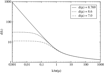
Figure 5: Solution for the ghost form function $d(k)$ for different renormalization constants $d(\mu)=7.0,8.6$ and $8.716$.

The value of the remaining renormalization constant $d(\mu)$ has been specified as follows:

Consider the equation for the ghost form factor. The curvature $\bar{\chi}(k)$, the Coulomb form factor $f(k)$ as well as the renormalization constants $\bar{\xi}$ and $\bar{\chi}(\mu)$ do not enter this equation. Thus, for given $\bar{\omega}(k)$ the solution $d(k)$ depends only on the renormalization constant $d(\mu)$. Figure 5 shows the solution to the ghost form factor for various values of the renormalization constant $d(\mu)$ keeping $\bar{\omega}(k)$ fixed to the solution shown in figure 6. It is seen, that all solutions have the same ultraviolet behaviour independent of the renormalization constant $d(k)$. Furthermore, this ultraviolet behaviour is consistent with the asymptotic solutions (120) found in section V (Note, that a double logarithmic plot is used)! The infrared behaviour of $d(k)$ depends, however, on the actual value of $d(\mu)$. For $d(\mu)$ smaller than some critical value $d_{cr}$ the curves approach a constant for $k\to 0$. At a critical $d(\mu)=d_{cr}$ the ghost form factor diverges for $k\to 0$ and above the critical value $d>d_{cr}$ no solution to the ghost form factor exists. We have adopted the critical value $d(\mu)=d_{cr}$ as the physical value for the following reasons:

• In $D=3$ (which will be considered elsewhere) a self-consistent solution to the coupled Schwinger-Dyson equations exists only for this critical value.

• Only the critical value produces an infrared diverging ghost form factor.

• The diverging ghost form factor is in agreement with our analytic studies of the infrared limit of the Schwinger-Dyson equations considered in section V using the angular approximation (see eqs. (151)).

• The divergent ghost form factor gives rise to a linear rising confining potential as will be shown later on.

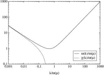
Figure 6: Solution for the gap function $\bar{\omega}(k)$ for $\bar{\xi}=0$

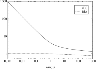
Figure 7: Ghost form function $d(k)$ and Coulomb correction $f(k)$ for $\bar{\xi}=0$

The critical $d(\mu)=d_{cr}$ is defined by $d^{-1}(k\to 0)\to 0$ which is referred to as “horizon condition” R19 . At the arbitrarily chosen (dimensionless) renormalization point $\bar{\mu}=0.32$ the critical renormalization constant is given by $d(\bar{\mu})=8.716$. In all self-consistent solutions presented in this paper we have adopted this critical value.
We have also investigated the dependence of the self-consistent solutions on the remaining renormalization constants $\hskip 2.84544pt\bar{\xi}$ and $\bar{\chi}(\mu)$ (recall, that $d,\bar{\omega}(\bar{k})$ are independent of $\hskip 2.84544pt\bar{\xi}$ and $\bar{\chi}(\mu)$). We have found, that our self-consistent solutions change by less then $0.01^{0}/_{00}$, when $\bar{\chi}(\mu)$ is varied in the intervall $[-1,1]$. Thus there is practically no dependence of our results on $\bar{\chi}(\mu)$. We have therefore put $\bar{\chi}(\mu)=0$ in all calculations.
Figures 8 and 9 show the self-consistent solution for $d(k)$ and $\bar{\omega}(k)$ for $\bar{\xi}=0,-0.5,-1.0$. Both quantities show only very slight variations with $\bar{\xi}$ up to a (dimensionless) momentum of order one. The ultraviolet behaviour is independent of $\bar{\xi}$ and in agreement with our analytic results obtained in section V. Furthermore, also the infrared behaviour of $d(k)$ and $\bar{\omega}(k)$ is independent of $\bar{\xi}$.

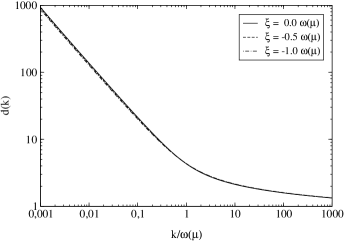
Figure 8: Ghost form function $d(k)$ for $\bar{\xi}=0,-0.5$ and $-1.0$ .

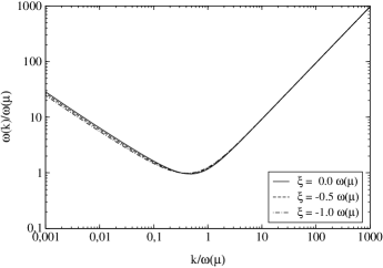
Figure 9: Gap function $\bar{\omega}(k)$ for $\bar{\xi}=0,-0.5$ and $-1.0$ .

Our analysis of the infrared behaviour of the solutions to the Schwinger-Dyson equations using the angular approximation given in section V has revealed, that in this approximation the critical exponents $\alpha$ and $\beta$ and the ratio $A/B^{2}$ of the amplitudes of $\bar{\omega}(k)$ and $d(k)$, see eq. (133), are independent of the renomalization constants $\hskip 2.84544pt\bar{\xi}$, $\bar{\chi}(\mu)$. Our numerical solutions confirm this result even without resorting to the angular approximation. Figure 10 shows these quantities $A/B^{2}$ and the infrared exponent (133) $\alpha$ as function of $\hskip 2.84544pt\bar{\xi}$. There is practically no dependence. We will therefore put $\hskip 2.84544pt\bar{\xi}=0$ in the further numerical calculations.

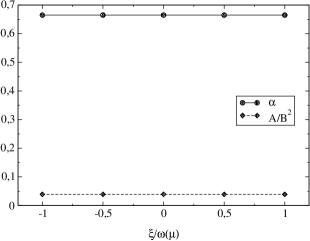
Figure 10: $A/B^{2}$ and $\alpha$ in dependence of $\bar{\xi}$

The obtained numerical results are all in qualitative agreement with our previous analytic investigations. For large $k\to\infty$ the gluon energy $\omega(k)\sim\sqrt{k^{2}}$ is that of a non-interacting boson and the curvature in orbit space $\chi(k)/\omega(k)\sim\frac{1}{\sqrt{\ln k/\mu}}$ vanishes asymptotically. This is in agreement with the expectations of asymptotic freedom. For $k\to 0$ the gluon energy $\omega(k)$ diverges reflecting the absence of free gluons in the infrared, which is a manifestation of confinement. While the gluon propagator $\frac{1}{\omega(k)}\to 0$ for $k\to 0$ is suppressed in the infrared the ghost propagator $d(k)/k^{2}$ diverges for $k\to 0$. It is worthwile noticing, that the same behaviour of the gluon and ghost propagators is obtained in covariant Schwinger-Dyson equations, derived from the functional integral in Landau gauge R21 , RX . From figure 6 it is seen, that for $k\to 0\hskip 2.84544pt\hskip 2.84544pt\hskip 2.84544pt\omega(k)$ approaches $\chi(k)$. As shown analytically in section V this is a generic feature of our gap equation and reflects the non-trivial metric of the space of gauge orbits (given by the Faddeev-Popov matrix). This non-trivial metric is crucial for the infrared behaviour of the theory and in particular for the confinement. This can be seen from figures 11, 12 , where we present the self-consistent solutions for $\omega(k)$ and $d(k)$, when the curvature of the gauge orbit space is neglected by putting $\chi(k)=0$ as done in R16 or when neglecting the curvature in the Coulomb term as done in R17 . In these cases the infrared behaviour of $\omega(k)$ is drastically different from the previous case, although we have still chosen the horizon condition $d^{-1}(k\to 0)=0$ as renormalization condition ($d(k)$ is still infrared divergent as can be read off from figure 12). In particular notice that $\omega(k\to 0)=\textrm{const.}$ when the curvature $\chi$ is completely neglected, i.e. $\alpha=0$ in eq. (133). From the two sum rules (144) for the infrared critical exponents follows $\beta=\frac{1}{2}$ and $\gamma=0$. Thus with the horizon condition as renormalization the neglect of the curvature in the Schwinger-Dyson equation yields $d(k)\sim\frac{1}{\sqrt{k}}$, $\omega(k)=\textrm{const.}$ and $\chi(k)=\textrm{const.}$ for $k\to 0$ .

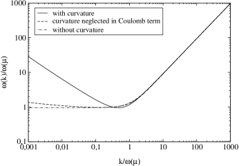
Figure 11: Consistent solution of the gap function $\bar{\omega}(k)$ for different treatments of the curvature for $\bar{\xi}=0$ .

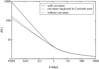
Figure 12: Consistent solution of the ghost form function $d(k)$ for different treatments of the curvature for $\bar{\xi}=0$ .

VIII The Coulomb potential

The vacuum expectation value of the Coulomb term of the Yang-Mills Hamiltonian can be interpreted as interaction potential between static color charge densities $\rho^{a}({\bf x})$. The static quark potential can therefore be extracted from this term by taking the vacuum expectation value and assuming, that the color charge density $\rho^{a}({\bf x})$ describes two static infinitely heavy color charges

$$\rho^{a}(x)=gq^{a}_{(1)}\delta\left({\bf x}-{\bf x}_{(1)}\right)+gq^{a}_{(2)}\delta\left({\bf x}-{\bf x}_{(2)}\right)$$ (174)

located at ${\bf x}_{(1)}$ and ${\bf x}_{(2)}$ and separated a distance ${\bf x}_{(1)}-{\bf x}_{(2)}={\bf r}$ apart. This yields

$$E_{C} = E^{(1)}_{C}+E^{(2)}_{C}+q^{a}_{(1)}V^{ab}\left({\bf x}_{(1)},{\bf x}_{(2)}\right)q^{b}_{(2)}\hskip 2.84544pt,$$ (175)

where $E^{(1,2)}_{C}$ are the (divergent) self-energies of the two separate static quarks and

$$V^{ab}\left({\bf x}_{(1)},{\bf x}_{(2)}\right)=g^{2}\langle\omega|F^{ab}\left({\bf x}_{(1)},{\bf x}_{(2)}\right)|\omega\rangle$$ (176)

is the static quark potential, with $F^{ab}\left({\bf x},{\bf x}^{\prime}\right)$ being the Coulomb propagator defined by eq. (17). In the above considered one-loop approximation the potential is color diagonal $V^{ab}=\delta^{ab}V$ and, with the explicit form of the Coulomb propagator, is given by

$$V\left({\bf r}\right)=\int\frac{d^{3}k}{(2\pi)^{3}}\frac{d(k)^{2}f(k)}{k^{2}}e^{i{\bf k}{\bf r}}=\int\frac{d^{3}k}{(2\pi)^{3}}e^{i{\bf k}{\bf r}}V(k).\hskip 2.84544pt\hskip 2.84544pt\hskip 2.84544pt\hskip 2.84544pt$$ (177)

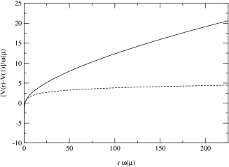
Figure 13: Coulomb Potential for $\bar{\xi}=0$ with (full line) and without inclusion of the curvature (dashed line).

Performing the integral over the polar angle, one finds

$$V(r)=\frac{1}{2\pi^{2}}\int\limits^{\infty}_{0}dk{d(k)^{2}f(k)}\frac{\sin(kr)}{kr}\hskip 2.84544pt.$$ (178)

Before presenting the numerical result for the Coulomb potential let us consider its asymptotic behaviour for $k\to 0$ and $k\to\infty$. In section V.2 we have found the infrared behaviour $f(k\to 0)=$ const. and $d(k\to 0)\sim\frac{1}{k}$. This yields precisely a linearly rising Coulomb potential $V(k)\sim 1/k^{4}$. Furthermore for $k\to\infty$ the ghost form factor was found to behave as (see eq. (120) $d(k)\sim\frac{1}{\sqrt{\ln k/\mu}}$. Adopting the leading order expression for the Coulomb form factor (see eq. (73) and figure 3) $f(k)=1$ we find

$$k^{2}V(k)\sim\frac{1}{\ln k/\mu}\hskip 2.84544pt,\hskip 2.84544ptk\to\infty\hskip 2.84544pt.$$ (179)

This is precisely the behaviour found in ref. R25 in one-loop perturbation theory.
The Coulomb potential calculated from the numerical solution to the coupled Schwinger-Dyson equations is shown in figure 13. At small distance it is dominated by an ordinary $\sim\frac{1}{r}$ potential, while at large distances it raises almost linearly. The numerical analysis shows, that its Fourier transform behaves for $k\to 0$ like $1/k^{3.7}$, while a strictly linearising potential would require a $1/k^{4}$ dependence (In ref. R30 the power $1/k^{3.6}$ was found). When the curvature is neglected the gluon energy becomes infrared finite and the Coulomb potential approaches a constant at $r\to\infty$. Thus both quark and gluon confinement is lost when the curvature of the space of gauge orbits is discarded.

IX Summary and Conclusions

In this paper we have solved the Yang-Mills Schrödinger equation for the vacuum in Coulomb gauge by the variational principle using a trial wave function for the Yang-Mills vacuum, which is strongly peaked at the Gribov horizon. Such a wave functional is recommended by the fact, that the dominant infrared field configurations lie on the Gribov horizon. Such field configurations include, in particular, the center vortices, which have been identified as the confiner of the theory. With this trial wave function the vacuum energy has been evaluated to one-loop order. Minimization of the vacuum energy has led to a system of coupled Schwinger-Dyson equations for the gluon energy, the ghost and Coulomb form factor and for the curvature in orbit space. Using the angular approximation these Schwinger-Dyson equations have been solved analytically in both, the infrared and the ultraviolet regime. In the latter case, we have found the familiar perturbative asymptotic behaviours. In the infrared the gluon energy diverges indicating the absence of free gluons at low energies, which is a manisfestation of confinement. The ghost form factor is infrared diverging and gives rise to a linear rising static quark potential. The asymptotic analytic solutions for both $k\to 0$ and $k\to\infty$ are reasonably well reproduced by the full numerical solutions of the coupled Schwinger-Dyson equations. Our investigations show, that the inclusion of the curvature, i.e. the proper metric of orbit space, given by the Faddeev-Popov determinant is crucial in order to obtain the confinement properties of the theory. When the curvature is discarded (using a flat space of gauge connnections) free gluons exist even for $k\to 0$ and the static quark potential is no longer confining.

The results obtained in the present paper are quite encouraging and call for further studies. In a subsequent paper we will investigate along the same lines the $2+1$-dimensional Yang-Mills theory, which (up to a Higgs field) can be considered as the high temperature limit of the $3+1$-dimensional theory. It would be also interesting to calculate the spatial Wilson loop in order to check whether the relation $\sigma_{coul}\approx 3\sigma$ found on the lattice R26 is reproduced. Furthermore, the spatial t’Hoft loop should be calculated using the continuum representation derived in R29 . Eventually one should include dynamical quarks, since the ultimate goal should be the description of the physical hadrons.

Note added

After this work was completed we have been able to show that the infrared limit of the Yang-Mills wave functional (36) is independent of the power $\alpha$ of the Faddeev-Popov determinant R100 .

References

• (1) D.J. Gross and F. Wilczek, Phys. Rev. D8 (1973) 3633
H.D. Politzer, Phys. Rev. Lett. 30 (1973) 1346
Phys. Rept. 14 (1974) 129
• (2) M. Creutz. Phys. Rev. D21 (1980) 2308
• (3) Y. Nambu, Phys. Rev. D10 (1974) 4262
S. Mandelstam, Phys. Lett. B53 (1974) 476
G. Parisi, Phys. Rev. D11 (1975) 970
Z.F. Ezawa and H.C. Tze, Nucl. Phys. B100 (1976) 1
R. Brout, F. Englert and W. Fischler, Phys. Rev. Lett. 36 (1976) 649
F. Englert and P. Windey, Nucl. Phys. B135 (1978) 529
G. ’t Hooft, Nucl. Phys. B190 (1981) 455: Phys. Scr. 25 (1981) 133
• (4) G. ’t Hooft, Nucl. Phys. B138 (1978) 1
G. Mack and V.B. Petkova, Ann. Phys. (NY) 123 (1979) 442
G. Mack, Phys. Rev. Lett. 45 (1980) 1378
G. Mack and V.B. Petkova, Ann. Phys. (NY) 125 (1980) 117
G. Mack, in: Recent Developments in Gauge Theories, eds. G. ’t Hooft et al. (Plenum, New York, 1980)
G. Mack and E. Pietarinen, Nucl. Phys. B205 [FS5] (1982) 141
Y. Aharononv, A. Casher and S. Yankielowicz, Nucl. Phys. B146 (1978) 256
J.M. Cornwall, Nucl. Phys. B157 (1979) 392
H.B. Nielsen and P. Olesen, Nucl. Phys. B160 (1979) 380
J. Ambjørn and P. Olesen, Nucl. Phys. B170 (1980) 60, 265
E. T. Tomboulis, Phys. Rev. D23 (1981) 2371
• (5) J. Greensite, hep-lat/0301023
• (6) T. Suzuki, I. Yotsuyanagi, Phys. Rev. D42 (1990) 4257
S. Hioki et al. Phys. Lett. B272 (1991) 326
G. Bali, Ch. Schlichter, K. Schilling, Prog. Theor. Phys. Suppl. 131 (1998) 645 and refs. therein
• (7) L. DelDebbio, M. Faber, J. Greensite, S. Olejnik, Phys. Rev. D55 (1997) 2298
K. Langfeld, H. Reinhardt, O. Tennert, Phys. Lett. B419 (1998) 317
M. Engelhardt, K. Langfeld, H. Reinhardt, O. Tennert, Phys. Rev. D61 (2000) 054504
• (8) V.N. Gribov, Nucl. Phys. B139 (1978) 1
• (9) D. Zwanziger, Nucl. Phys. B378 (1992) 525
• (10) A. Cuccheri and D. Zwanziger, Phys. Rev. D65, 014001 (2002)
• (11) J. Greensite, Š. Olejnik and D. Zwanziger, hep-lat/0401003
• (12) see e.g. the Proceedings of “Lattice 2002” and “Lattice 2003”
• (13) C. Callan, R. Dashen, D. Gross, Phys. Rev. D17 (1978) 2717, D19 (1979) 1826, D20 (1979) 3279
D. Gross, R. Pisarski, L. Yaffe, Rev. Mod. Phys. 53 (1981) 43
• (14) I.H. Duru and H. Kleinert, Phys. Lett. B84 (1979) 30
• (15) R. Jackiw, Rev. Mod. Phys. 52 (1980) 661
• (16) C. Feuchter and H. Reinhardt, hep-th/0402106
• (17) K. Johnson, The Yang-Mills Ground State, in: QCD - 20 years later, vol. 7, p. 795,
eds. P.M. Zerwas and H.A. Kastrup
D.Z. Freedman, P.E. Haagensen, K. Johnson and J.-I. Latorre, Nucl. Phys.
M. Bauer, D.Z. Freedman, P.E. Haagensen, Nucl. Phys. B428 (1994) 147
• (18) J. Goldsone, R. Jackiw, Phys. Lett. B74 (1978) 81
V. Baluni, B. Grossman, Phys. Lett. B78 (1978) 226
A. Izergin et al., Teor. Mat. Fiz. 38 (1979) 3
• (19) N.H. Christ and T.D. Lee, Phys. Rev. D22 (1980) 939; Phys. Scripta 23 (1981) 970
T.D. Lee, Particle Physics and Introduction to Field Theory, Hardwood Academic, Chur, 1981
• (20) F. Lenz, H.W.L. Naus, M. Thies, Ann. Phys. 233 (1994) 317
H. Reinhardt, Phys. Rev. D55 (1997) 2331
• (21) I.L. Kogan and A. Kovner, Phys. Rev. D52 (1995) 3719
C. Heinemann, C. Martin, E. Jancu and D. Vautherin, Phys. Rev. D61 (2000) 116008
O. Schröder and H. Reinhardt, hep-ph/0207119; Annals Phys. 307 (2003) 452 hep-ph/0306244
• (22) H. Reinhardt, Mod. Phys. Lett. A11 (1996) 2451,
H. Reinhardt, Nucl. Phys. B503 (1997) 505
• (23) A.P. Szczepaniak and E.S. Swanson, Phys. Rev. D65 (2002) 025012
• (24) A. P. Szczepaniak, Phys. Rev. D69, (2004) 074031
• (25) J.P. Greensite, Nucl. Phys. B166 (1980) 113
• (26) D. Zwanziger, Nucl. Phys. B518 (1998) 237
• (27) M. E. Peskin and D. V. Schroeder, An Introduction to quantum field theory, Addison-Wesley (1985)
• (28) R. Alkofer and L. v. Smekal, Phys. Rep. 353 (2001) 281
• (29) C.S. Fischer, R. Alkofer, H. Reinhardt, Phys. Rev. D65 (2002) 094008
C.S. Fischer, R. Alkofer, Phys. Lett. B536 (2002) 177
• (30) A. Cuccheri and D. Zwanziger, Phys. Rev. D65, 014002 (2002)
• (31) A.R. Swift, Phys. Rev. D38 (1988) 668
• (32) C. Lerche and L. v. Smekal, Phys. Rev. D65 (2002) 125006
D. Zwanziger, Phys. Rev. D65 (2002) 094039
• (33) H. Reinhardt, Phys. Lett. B557 (2003) 317
• (34) D. Zwanziger, hep-ph/0312254
• (35) H. Reinhardt and C. Feuchter, On the Yang-Mills wave functional in Coulomb gauge, hep-th/0408237