Planar Skyrmions: Vibrational Modes and Dynamics

Abstract

We study Skyrmion dynamics in a (2+1)-dimensional Skyrme model. The system contains a dimensionless parameter $\alpha$, with $\alpha=0$ corresponding to the O(3) sigma-model. If two Skyrmions collide head-on, then they can either coalesce or scatter — this depends on $\alpha$ and on the incident speed $v$, and is affected by transfer of energy to and from the internal vibrational modes of the Skyrmions. We classify these internal modes and compute their spectrum, for a range of values of $\alpha$. In particular, we find that there is a fractal-like structure of scattering windows, analogous to those seen for kink-antikink scattering in 1+1 dimensions.

1 Introduction

In this paper, we investigate aspects of the dynamics of the planar Skyrme system, in which the field configuration is a map from ${\bf R}^{2}$ to $S^{2}$. In particular, we examine the discrete vibrational modes of static $N$-Skyrmion solutions. Such modes correspond to relatively long-lived vibrational states. They are of importance for semiclassical quantization (see, for example, [19, 2] for the Skyrme case, [20] for the planar-Skyrme case); but our interest lies in their effect on the classical dynamics of Skyrmions.

A long-standing prototype is the $\phi^{4}$ system in $1+1$ dimensions. Here the soliton is a kink (or antikink), which possesses a single internal oscillatory mode. If a kink and an antikink approach each other with low relative speed $v<v_{0}$, then they form a long-lived ‘breather’ or bion state [9]. (This is not an exact breather, and eventually decays.) If, on the other hand, the kink and the antikink approach at high speed $v>v_{1}$, then they bounce off each other, and each escapes to infinity (the collision is inelastic, with some radiation being emitted). For intermediate impact speed $v_{0}<v<v_{1}$, there is a fractal-like structure of ‘reflection windows’, with trapping and reflection alternating [4, 3, 1]. This can be understood in terms of a resonant energy exchange between the translational motion of the kink and its internal oscillation [4]. Also worth mentioning is that the internal mode can in some sense be ‘extrapolated’ to a non-infinitesimal dynamical process, namely a kink-antikink-kink collision [14].

In this paper, we shall study analogous features for the (2+1)-dimensional Skyrme system. There are several significant differences between this case and that of kinks. The first is that two kinks (as opposed to a kink and an antikink) always repel each other, and there is no static 2-kink solution; whereas for Skyrmions (with a suitable choice of potential) static 2-Skyrmion solutions do exist. Consequently, it makes sense to study Skyrmion-Skyrmion collisions: for head-on collisions, one might expect that there will be a critical speed $v_{0}$ such that

• for impact speed $v<v_{0}$, the Skyrmions coalesce to form a 2-Skyrmion;

• for $v>v_{0}$, the Skyrmions scatter and each escapes to infinity;

and the internal modes should play a role in this process.

As we shall see, however, the picture is not quite as simple as this. The system contains a dimensionless parameter $\alpha$, and the various dynamical features depend crucially on $\alpha$. We study numerically how the spectrum of vibrational modes, and the scattering behaviour, vary with $\alpha$. For small $\alpha$, internal modes are absent, and the picture is indeed as suggested above: coalescence for $v<v_{0}$, and scattering for $v>v_{0}$. But for larger $\alpha$, a rich spectrum of internal modes appears, and the scattering behaviour also becomes more complex. In particular, there is a range of $\alpha$ within which one sees a fractal-like structure of ‘scattering windows’, separated by regions of coalescence.

2 The planar Skyrme system

The Skyrme system in ${\bf R}^{2+1}$ is defined as follows. Let $x^{\mu}=(x^{0},x^{1},x^{2})=(t,x,y)$ denote the standard space-time coordinates; indices are raised and lowered using the standard Minkowski metric (with signature $+--$). The two spatial coordinates are denoted $x^{j}$. The Skyrme field is a unit vector field $\vec{\phi}=(\phi_{1},\phi_{2},\phi_{3})$, with $\vec{\phi}\cdot\vec{\phi}=1$. Its space-time and spatial derivatives are denoted $\partial_{\mu}\vec{\phi}$ and $\partial_{j}\vec{\phi}$ respectively. The Lagrangian density is

$${\cal L}={\scriptstyle\frac{1}{2}}(\partial_{\mu}\vec{\phi})\cdot(\partial^{\mu}\vec{\phi})-{\scriptstyle\frac{1}{4}}\gamma\Omega_{\mu\nu}\Omega^{\mu\nu}-{\scriptstyle\frac{1}{2}}\alpha V(\phi_{3})\,,$$ (1)

where $\Omega_{\mu\nu}$ is the triple scalar product $\Omega_{\mu\nu}=\vec{\phi}\cdot(\partial_{\mu}\vec{\phi})\times(\partial_{\nu}\vec{\phi})$, $V$ is a function of $\phi_{3}$, and $\alpha$ and $\gamma$ are constants.

The boundary condition at spatial infinity is $\vec{\phi}\to(0,0,1)$ as $r\to\infty$, where $r^{2}=x^{2}+y^{2}$. A configuration satisfying the boundary condition has an integer winding number, which we denote $N$, and which is given by

$$N=\frac{1}{4\pi}\int\Omega_{12}\,d^{2}x\,.$$ (2)

The static energy $E$ of a configuration is

$$E=\frac{1}{2}\int\left[(\partial_{j}\vec{\phi})\cdot(\partial_{j}\vec{\phi})+\gamma(\Omega_{12})^{2}+\alpha V(\phi_{3})\right]\,d^{2}x\,.$$ (3)

The quantity $(\gamma/\alpha)^{1/4}$ has units of length, and so we shall henceforth fix the length scale by taking $\gamma=\alpha$. So we have a system depending on the parameter $\alpha$, as well as on the function $V(\phi^{3})$. The static energy of a configuration with winding number $N$ satisfies the Bogomol’nyi bound [7, 6]

$$E\geq 4\pi|N|\left(1+\frac{\alpha}{2}\int_{-1}^{1}\sqrt{V(\phi)}\,d\phi\right)\,.$$ (4)

Clearly for finite energy we need $V(1)=0$. In the asymptotic region $r\gg 1$, the two components $\phi_{1}$ and $\phi_{2}$ (which are the analogues of the three pion fields in the full Skyrme model) satisfy a Klein-Gordon equation where the ‘pion mass’ $m$ is given by $m^{2}=-\alpha V^{\prime}(1)/2$. So the frequency $\omega$ of radiation is bounded below by $m$. Two choices of $V(\phi)$ for which the corresponding systems have been investigated in some detail [17, 18, 11, 21, 16] are $V(\phi)=1-\phi$ and $V(\phi)=1-\phi^{2}$; we refer to these as Old Baby Skyrme (OBS) and New Baby Skyrme (NBS), respectively [21]. We shall restrict our attention to these two systems, concentrating especially on the NBS case; note that previous work on semiclassical quantization [20] dealt with the OBS case.

We remark in passing on the $\alpha\to\infty$ limit, which amounts to deleting the $(\partial_{\mu}\vec{\phi})^{2}$ term in the Lagrangian [15]. This system may admit stable solitons. For example, if $V(\phi)=1-\phi$, then there is a solution which has compact support (ie. $\phi^{3}\cong 1$ outside a disc of finite radius), and which does not saturate the Bogomol’nyi bound [5]. With $V(\phi)=(1-\phi)^{2}$, on the other hand, one has a smooth static rotationally-symmetric solution with $\phi^{3}=1-2\exp(-r^{2}/2N)$, which does saturate the Bogomol’nyi bound. See [15] for a more general discussion.

The simplest Skyrmion solutions are rotationally-symmetric, or more accurately O(2)-symmetric. Letting $r$ and $\theta$ represent the usual polar coordinates on ${\bf R}^{2}$, we say that a configuration $\vec{\phi}(r,\theta)$ is O(2)-symmetric if

• $\phi_{3}=\phi_{3}(r)$ with $\phi_{3}(\infty)=1=|\phi_{3}(0)|$; and

• $\phi_{1}+{\rm i}\phi_{2}=F(r)\exp({\rm i}N\theta)$ with $F(r)$ real-valued.

Here $N$ is an integer. Note that we necessarily have $F(\infty)=0=F(0)$. An equivalent definition is to say that $\vec{\phi}$ has the ‘hedgehog’ form

$$\vec{\phi}(r,\theta)=\bigl{(}\sin(f)\cos(N\theta),\sin(f)\sin(N\theta),\cos(f)\bigr{)}\,,$$ (5)

where the profile function $f=f(r)$ is smooth and real-valued with $f(\infty)=0$ and $f(0)=K\pi$ for some positive integer $K$. There exist symmetric solutions with $K>1$, but they are unstable [11]; so we shall restrict our attention here to the case $K=1$. In this case, $N$ is the same as the winding number (2) [17]. For the NBS system, there is considerable numerical evidence that, for each $N$, there is a smooth minimal-energy $N$-Skyrmion solution, and this solution is O(2)-symmetric. For $\alpha=1$, the normalized energy $E_{N}=E/(4\pi N)$ of this $N$-Skyrmion for $1\leq N\leq 4$, obtained by numerical minimization, is as follows: $E_{1}=2.15$, $E_{2}=1.91$, $E_{3}=1.85$, $E_{4}=1.83$. (Note that the Bogomol’nyi bound (4) is $E_{N}\geq 1.7854$.) Since $E_{N}$ is a decreasing function of $N$, we expect Skyrmions to coalesce; in particular, a low-speed collision of two 1-Skyrmions will result in a single 2-Skyrmion.

3 Vibrational modes of the $N$-Skyrmion

In this section, we study the spectrum of vibrations about O(2)-symmetric Skyrmion solutions. The set of all perturbations about a symmetric configuration is a vector space which is acted on by O(2), and which therefore decomposes into disjoint subspaces corresponding to representations of O(2). We begin, therefore, with a brief summary of the irreducible representations of O(2) in this context.

The group O(2) is generated by the rotations $\theta\mapsto\theta+c$, which make up SO(2); and the reflections $\theta\mapsto-\theta$. It has two 1-dimensional irreducible representations $\langle+\rangle$ and $\langle-\rangle$; and for each positive integer $p$, a 2-dimensional irreducible representation $\langle p\rangle$, containing two degenerate modes $\langle p,+\rangle$ and $\langle p,-\rangle$. The corresponding perturbations $\delta\vec{\phi}$ of $\vec{\phi}$ have the following form.

$\langle+\rangle$:

$\delta\vec{\phi}=\bigl{(}A\cos(N\theta),A\sin(N\theta),B\bigr{)}$, with $A\sin f+B\cos f=0$;

$\langle-\rangle$:

$\delta\vec{\phi}=\bigl{(}-A\sin(N\theta),A\cos(N\theta),0\bigr{)}$;

$\langle p,+\rangle$:

$\delta\phi_{1}=B\cos[(N-p)\theta)]+C\cos[(N+p)\theta)]$,
$\delta\phi_{2}=B\sin[(N-p)\theta)]+C\sin[(N+p)\theta)]$,
$\delta\phi_{3}=A\cos(p\theta)$, with $(B+C)\sin f+A\cos f=0$.

$\langle p,-\rangle$:

$\delta\phi_{1}=-B\sin[(N-p)\theta)]-C\sin[(N+p)\theta)]$,
$\delta\phi_{2}=B\cos[(N-p)\theta)]+C\cos[(N+p)\theta)]$,
$\delta\phi_{3}=-A\sin(p\theta)$, with $(B+C)\sin f+A\cos f=0$.

Clearly $\langle+\rangle$ consists of perturbations which maintain the hedgehog form (5): the profile of the Skyrmion changes, but it remains O(2)-symmetric. And $\langle-\rangle$ consists of perturbations which allow $F(r)$ to become complex-valued but preserve its modulus (in other words, $F$ acquires an $r$-dependent phase). So $\langle-\rangle$ includes the zero-mode $\phi_{1}+{\rm i}\phi_{2}\mapsto\exp{({\rm i}\chi)}(\phi_{1}+{\rm i}\phi_{2})$, where $\chi$ is a constant phase angle. The other zero-modes are the translations in space; these form a doublet which belongs to the representation $\langle 1\rangle$. Apart from shape modes in $\langle+\rangle$, some other particularly significant positive modes (cf. [19, 2] for the (3+1)-dimensional Skyrme case) are ‘dipole breather’ modes belonging to $\langle 1\rangle$, which correspond to the Skyrmion oscillating from one side to the other; and the ‘splitting mode’ of the 2-Skyrmion into two single Skyrmions, which belongs to $\langle 2\rangle$.

The spectrum of oscillations around a static solution will consist of the zero-modes mentioned above (angular frequency $\omega=0$); a continuum of radiation modes ($\omega>m$); a finite number of negative modes ($\omega$ imaginary) if the solution is unstable; and a finite, possibly zero, number of discrete positive modes ($0<\omega<m$).

We have used two, very different, numerical methods to compute the vibration spectrum. The first involves deriving the relevant Sturm-Liouville equation (in $r$) for each of the classes $\langle+\rangle$, $\langle-\rangle$, $\langle 1\rangle$, $\langle 2\rangle,\ldots$; this is then solved using a Chebyshev spectral method. This method can be used for unstable as well as stable solutions. The second method involves a full (2+1)-dimensional simulation of the field equations, and only works for vibrations about stable solutions. The procedure is to construct a static Skyrmion (by relaxation), put in a perturbation, solve the time evolution for a long time interval, extract a time-series by sampling the field at some point in space, and finally Fourier-analyse this data. See, for example, ref [2], where this method was used for the (3+1)-dimensional Skyrme system. The results of the two methods are consistent.

Let us now look at the internal modes of the 1-Skyrmion in both the OBS and NBS systems. The results are summarized in Figure 1, where the modes can be seen ‘peeling off’ the bottom of the continuum band as $\alpha$ increases. For the OBS system (where $m^{2}=\alpha/2$), there are no internal modes if $\alpha<1$. The first mode to appear belongs to $\langle 1\rangle$, followed by modes in $\langle 2\rangle$, $\langle-\rangle$ and $\langle+\rangle$ in that order. For the NBS system (where $m^{2}=\alpha$), the first mode (again in $\langle 1\rangle$) appears at $\alpha\approx 0.27$, followed by a mode in $\langle+\rangle$ (at $\alpha\approx 0.30$). The latter crosses over the former at $\alpha\approx 0.31$; but at $\alpha\approx 1.2$, the modes cross again, and the $\langle 1\rangle$ mode has the lower frequency for $\alpha>1.2$. The number of modes grows quite rapidly with $\alpha$.

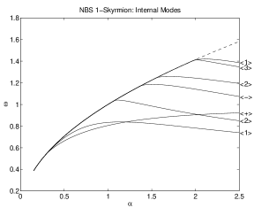
Figure 1: Frequencies of the internal modes of the 1-Skyrmion.

In the OBS system, the 2-Skyrmion is stable; for all $\alpha>0$, it has a discrete positive mode in $\langle 2\rangle$, corresponding to the breakup of the 2-Skyrmion into two single Skyrmions (‘splitting mode’). As $\alpha$ increases, more positive modes appear. The 3-Skyrmion in the OBS system is unstable [17]; there is always a negative mode, which belongs to $\langle 2\rangle$. From now on, we consider the NBS system only.

For the NBS system with $\alpha=1$, the positive discrete modes of the 1-Skyrmion and the 2-Skyrmion are as follows.

$N=1$:

a shape mode (in $\langle+\rangle$) with $\omega=0.806$; and a dipole breather doublet in (in $\langle 1\rangle$) with $\omega=0.834$. See the right-hand diagram in Figure 1.

$N=2$:

a shape mode with $\omega=0.519$; a dipole breather doublet with $\omega=0.613$; a splitting doublet with $\omega=0.398$; and two further doublets (one in $\langle 2\rangle$ with $\omega=0.909$ and one in $\langle 3\rangle$ with $\omega=0.912$). See the right-hand diagram in Figure 3.

4 Skyrmion-Skyrmion scattering

In the NBS system, solitons attract each other, and the lowest-energy $N=2$ configuration corresponds to two superimposed solitons. This means that if two solitons are released from rest at finite separation, they slowly move towards each other to form a large lump. When simulating this numerically, we see that after the scattering, the solitons emerge at $90^{\circ}$, but their mutual attraction slows them down and forces them to move back towards each other. They then merge again and scatter in their initial direction, but stop again and keep oscillating back and forth. As the interaction is non-elastic, the lumps emit waves that carry away some energy. As a result, the amplitude of oscillation slowly decreases, and the configuration converges toward the two-soliton static configuration.

If the solitons are sent toward each other with a large-enough speed, they momentarily merge to form a large lump, and then two lumps emerge at $90^{\circ}$ and move away from each other. If the initial speed is too small, then these solitons do not escape from their mutual attraction, and they eventually form a single lump after several oscillations.

This behaviour suggests that there is a critical speed below which the solitons merge, and above which they escape. In Figure 2, we present the dependence of the critical speed $v$ (defined below) on the coupling constant $\alpha$. In the limit $\alpha\to 0$, the system is the O(3) sigma model, and a head-on collision always results in $90^{\circ}$ scattering [13, 12]. In other words, we expect that $v\to 0$ as $\alpha\to 0$, and this is consistent with the numerical results. For small $\alpha$, the Skyrmions scatter very easily; but as $\alpha$ increases towards $0.27$, they have an increasing tendency to coalesce. In a collision between Skyrmions, any positive discrete (localized) mode of the Skyrmion will inevitably be excited (cf. [3, 8]); this removes translational kinetic energy from each Skyrmion, and transfers it to an internal excitation which eventually decays into radiation. So when the shape mode appears (at $\alpha=0.27$), it very efficiently removes translational energy from the Skyrmions, and leaves them in a bound state. There is a partial effect even below $\alpha=0.27$, which can perhaps be understood in terms of a quasimode (cf. [8]): an ‘internal’ mode which is embedded within the continuum spectrum, and which becomes the shape mode when $\alpha$ increases beyond $0.27$.

On the other hand, for $\alpha$ larger than about $0.7$, the critical speed decreases. Between these two extremes, there is a region where the critical speed is close to the speed of light ($1$ in our units); but as scattering two solitons numerically at large speed is quite difficult, we were not able to determine the critical speed when $0.27<\alpha<0.7$, or determine for which value of $\alpha$ the $90^{\circ}$ scattering never takes place.

Figure 2: Critical velocity as a function of $\alpha$ for the NBS model.

If one looks closely at Figure 2, one notices that the curve folds back around the value $\alpha=0.263$. In that region, the solitons merge when the initial speed is either below the lowest value or above the largest one. The numerical simulations from which Figure 2 was obtained involve the head-on collision of two Skyrmions in their most attractive mutual orientation (the ‘attractive channel’), and with each having equal initial speed. The critical speed $v$ plotted in Figure 2 is defined as the speed below which the solitons always merge, except for the top part of the folding where it is defined as the speed above which the solitons always merge.

When $\alpha$ is slightly smaller than $0.263$, and when the initial speed is slightly above the lower critical value, we observed numerically that the scattering behaviour of the solitons can have a complex pattern for some values of $\alpha$. Instead of simply escaping or merging, the solitons swing back and forth as if they were slowly merging, but eventually they escape at $90^{\circ}$ or in the direction from which they came.

To describe this process, we can define the ‘scattering number’ as the number of times the two solitons scatter at $90^{\circ}$, and define it as zero when the solitons coalesce. So when the initial speed is very large, the scattering number is $1$ (except for the narrow range of $\alpha$ around $0.26$, where high-speed solitons coalesce). When the scattering number is even, the solitons scatter in the direction they came from; and when it is odd, they scatter at $90^{\circ}$. For a range of values of $\alpha$, the scattering number is very sensitive to the initial velocity, and exhibits a fractal-like structure.

The structure of the data is described in Table 1, where we present the scattering number for various ranges of initial speed, sampled at regular intervals. Each digit in the large strings corresponds to the scattering number for a given value of $v$. The final string (which is split over two lines) should be read as a single merged string. The first digit in each string corresponds to the smallest value of $v$ (‘First $v$’ in the table), while the last digit corresponds to the largest value of $v$ (‘Last $v$’ in the table). The increment size in $v$ is given in the third column.

$\alpha$	First $v$	$v$ increment	Last $v$	Scattering Numbers
0.24	0.4705	0.0001	0.477
002222000000000222005000022000003220000200002002002030200000111111
$\alpha$	First $v$	$v$ increment	Last $v$	Scattering Numbers
0.24	0.4721	0.00001	0.4726
222222222222222220000000000000000500000555500000000
$\alpha$	First $v$	$v$ increment	Last $v$	Scattering Numbers
0.24	0.472428	0.000001	0.4725
0555555555000000000000000000000000000000000000000700000000000055555555555
$\alpha$	First $v$	$v$ increment	Last $v$	Scattering Numbers
0.25	0.49	0.0001	0.497
22222200000000002222200000000222250000022250000222000020002200200202002
$\alpha$	First $v$	$v$ increment	Last $v$	Scattering Numbers
0.25	0.493241	0.000001	0.49332
22222000000000000000005000000000500000005000000000005505555500000040055043333000
$\alpha$	First $v$	$v$ increment	Last $v$	Scattering Numbers
0.26	0.4905	0.0005	0.53
00002022203002000002222200000002220000022230002200002000220230202022200
$\alpha$	First $v$	$v$ increment	Last $v$	Scattering Numbers
0.26	0.5156	0.000005	0.5159
2222222222222222222222222222220000000003000300000003330000000
$\alpha$	First $v$	$v$ increment	Last $v$	Scattering Numbers
0.26	0.51578	0.000001	0.515872
0300000000000333400000000000000000333333040000000000000000000000000000
00005333333333333334040

Table 1: Scattering numbers for a range of $\alpha$ and $v$.

One clearly sees that for the values of $\alpha$ given in Table 1, there is no sharp transition between scattering and the merging of solitons, but that instead there are several windows of initial speed where the solitons scatter several times before escaping at $90^{\circ}$ or in their original directions; these windows are separated by regions where the solitons do not escape. As the scattering number increases, the width of the windows become smaller, but the structure at any scale seems to be similar. One can also see in Table 1 that often, at the edge of a given window, there is a narrower window for a larger scattering number; this is not always the case, but we have observed this many times.

We should also point out that the scattering patterns given in Table 1 form a small subset of the range of scattering velocities that we have investigated numerically. We have observed a fractal structure in the scattering data for the range of speed contained between the lower and upper branch of the critical speed on Figure 2 when $\alpha$ was just below $0.26$. When $\alpha=0.24$, the windows were not as rich in structure as for $\alpha=0.26$, exhibiting large gaps of coalescence between the regions of multiple scattering.

5 Scattering and Vibration Modes

Our observations are analogous to those described by Anninos et al [1] in their study of kink-antikink scattering in the $\phi^{4}$ model in one dimension, where the scattering also exhibits windows of scattering separated by regions where a long-lived bound state is formed.

It is interesting to note that in Figure 2, the value $\alpha=0.263$ where the critical speed curls over is just below the value $\alpha=0.265$ where the breather mode $\langle 1\rangle$ emerges from the continuum band. Moreover, the curve for the shape mode $\langle+\rangle$ emerges at $\alpha=0.295$, and the curves for the two modes cross at $\alpha=0.310$. See Figure 3.

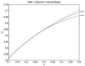
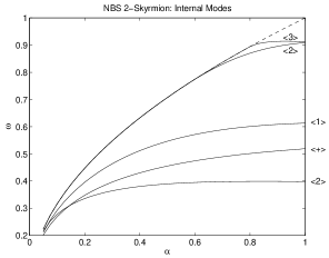
Figure 3: The frequencies of the internal modes of the $N=1$ and $N=2$ Skyrmions.

We also notice from Figure 3 that a splitting mode in $\langle 2\rangle$ (although not the lowest one) peels off from the continuum band at $\alpha=0.62$, and this is approximately the value (cf Figure 2) above which the solitons can scatter, suggesting that this splitting mode is implicated in the large-$\alpha$ part of Figure 2.

To understand the relation between the vibration modes and the scattering of solitons, we must first realise that during the scattering process the solitons are excited in various vibration modes. When they are sufficiently far apart, each lump can be considered as a single Skyrmion; while when they overlap, they form a configuration close to the $N=2$ rotationally-symmetric solution. Between these two configurations, they form intermediate states that extrapolate between the two extreme configurations, but that are difficult to describe. One thing that can be inferred from the expressions for $\delta\vec{\phi}$ is that the mode $\langle p\rangle_{1}$ for the 1-Skyrmion becomes the mode $\langle 2p\rangle_{2}$ for the 2-Skyrmion, as the two Skyrmions merge. For example, the dipole breather mode $\langle 1\rangle_{1}$ for each incident 1-Skyrmion becomes the splitting mode $\langle 2\rangle_{2}$ for the 2-Skyrmion, as the Skyrmions coalesce. More precisely, the lowest state for $\langle 1\rangle_{1}$ which is the translation mode of the 1-Skyrmion becomes the lowest-state of the $\langle 2\rangle_{2}$ mode. The first excited state of the $\langle 1\rangle_{1}$ mode, shown in Figures 1 and 3, transforms into the first excited state for the $\langle 2\rangle_{2}$ mode, which (as shown in Figure 3) crosses the mass threshold around $0.62$.

Moreover, due to the nonlinear nature of the model, the different vibration modes exchange some energy during the scattering. In particular, this means that some kinetic energy is transfered from the translation mode into the various vibration modes, and the reverse is also true when the two Skyrmions try to escape from their mutual attraction.

During the scattering, the vibration modes that are excited vary with time and depend on the overlap between the Skyrmions; but when the initial speed is close to the critical value, we observed that the vibration period is less than the characteristic time of scattering, implying that the system has plenty of time to oscillate.

We should also point out that all the scatterings that we have simulated numerically involved head-on collisions in the attractive channel [18], which means in particular that $\vec{\phi}$ was invariant under the rotation $\theta\mapsto\theta+\pi$. This implies that the modes $\langle p\rangle$ of the 2-Skyrmion, with $p$ odd, were never excited.

We thus see that when $\alpha<0.265$, there is no internal mode to excite the 1-Skyrmion, and the oscillation of the Skyrmions induced by their scattering is radiated away. When $\alpha>0.265$, the $\langle 1\rangle_{1}$ is excited during the scattering and it can absorb progressively larger amounts of energy. As the Skyrmions merge, this mode transforms into the first exited $\langle 2\rangle_{2}$ mode which is well above the mass threshold. The energy is thus radiated away and the scattering does not take place. When $\alpha>0.65$, the $\langle 2\rangle_{2}$ is a bound state, hence the energy is not radiated away and the $90^{\circ}$ scattering becomes possible again.

To try to predict the critical velocity shown in Figure 2, we now consider a simple model for the two-soliton scattering process, namely the dynamics of two equal masses, connected by a spring, on a cone. The cone corresponds to the moduli space for the two Skyrmions in their symmetric configuration [10], while the two masses connected by the spring models a single internal mode of oscillation of a Skyrmion. Moreover, to model the attraction between the two Skyrmions, the two masses are made to evolve in a central potential, describing the binding energy of two Skyrmions. Each mass is equal to half the mass of a Skyrmion, and the masses are positioned so that the line joining them crosses the origin, ie the tip of the cone. In this picture, the Skyrmion scatters with its mirror image; and the move over the tip of the cone corresponds to a $90^{\circ}$ scattering once the cone is unfolded onto the plane.

The Lagrangian for this system is

$$L=\frac{1}{2}(M_{x}\dot{X_{1}}^{2}+M_{x}\dot{X_{2}}^{2})-V_{1}(X1-X2)-V_{2}(X_{1})-V_{2}(X_{2}),$$ (6)

where

$$V_{1}(x) = \frac{k}{2}(x-X_{0})^{2},$$

$$V_{2}(x) = -\frac{A}{2\cosh(\lambda x)}.$$ (7)

The constants $A$ and $\lambda$ are coefficients, depending on $\alpha$, which we will choose to model the two-soliton scattering as closely as possible. The parameter $X_{0}$ describes the size of the soliton; we will take $X_{0}=1$. Notice that the depth of $V_{2}$ is $A/2$; so given that there are two degrees of freedom, $A$ corresponds to the depth of the two-Skyrmion bound-state potential. The equations of motion are

$$M_{x}\ddot{X_{1}} = -k(X_{1}-X_{2})-\frac{A\lambda\sinh(\lambda X_{1})}{2\cosh^{2}(\lambda X_{1})},$$

$$M_{x}\ddot{X_{2}} = k(X_{1}-X_{2})-\frac{A\lambda\sinh(\lambda X_{2})}{2\cosh^{2}(\lambda X_{2})}.$$ (8)

The value of $k$ is chosen so that the frequency of oscillation between $X_{1}$ and $X_{2}$ is the frequency of the shape mode $\langle+\rangle$, namely $k/M_{x}=\omega_{<+>_{1}}$. The equation $\omega_{<+>_{1}}=0.30+0.63(1-\exp(-1.58\ \alpha))$ gives a good approximation. Note that our simple model does not distinguish between the different vibration modes; as the frequencies of the $\langle+\rangle$ $\langle 1\rangle$ modes are very similar, we have taken the former for convenience.

The parameters $A$ and $\lambda$ in the potential $V_{2}$ are determined as follows. For $A$ we take the depth of the potential, namely $A=1-E_{2}/(2E_{1})$, where $E_{2}$ is the energy of the two-soliton bound state and $E_{1}$ is the energy of a single soliton. In Figure 4 we show the $\alpha$-dependence of the binding energy $E_{2}/(2E_{1})$. The curve is well-approximated by the relation $E_{2}/(2E_{1})=1+0.12(\exp(-3.88\ \alpha)-1)+0.01\ \alpha$.

Figure 4: $\alpha$-dependence of the binding energy of two Skyrmions.

For $\lambda$, we impose the condition that the frequency of the small-amplitude oscillations for $V_{2}$ is equal to the frequency of the lowest splitting mode for the two-soliton bound state $\omega_{<2>_{2}}$. That frequency is well approximated by the expression $\omega_{<2>_{2}}=0.2+0.2(1-\exp(-3.875\ \alpha))-0.015\alpha$. We therefore have $\lambda=\omega_{<2>_{2}}(2M_{{\rm tot}}/A)^{1/2}$, where $M_{{\rm tot}}=2M_{x}$.

To be more realistic, we should have one oscillator for each vibration mode. One quick way to approximate this is to have $n_{0}$ decoupled oscillators which, to first approximation, have the same frequency. This will correspond to taking $2n_{0}$ points of mass $M_{x}/n_{0}$ linked in pairs by springs with elastic constant $k/n_{0}$. To preserve the total binding energy of the system we must also divide $A$ by $n_{0}$. This is actually equivalent to solving equation (8), after multiplying $\lambda$ by $n_{0}^{1/2}$.

To simulate a scattering, we set up the two masses so that they are separated by their equilibrium distance $X_{0}$, and so that their centre of mass is located at $x=10$. We then send both of them with the same speed towards the origin. The motion of the masses in the potential well stretches the string and results in some transfer of translation energy into the oscillator. The initial speed therefore has to be large enough for the two masses to go over the tip of the cone and escape towards $x=-\infty$. If the speed is too small, the two masses oscillate around the tip of the cone.

Using these parameters, we have determined the critical velocity for $n_{0}=1$ and $n_{0}=2$, as shown in Figure 5. It produces the correct shape of curve, ie one that looks like the inverse of a Morse potential, but the actual critical velocities are too small.

Figure 5: Critical speed for the 2-point model; one oscillator (bottom curve) and two oscillators (top curve)

This is explained by the fact our simple model does not take into account the radiation of energy. Otherwise, the shape of the curve is more or less explained by the shape of the binding energy of two Skyrmions, as shown in Figure 4. Where the well is deepest, around $\alpha=1$, more energy is transferred into the oscillator, and the critical speed is high.

The drop in the critical velocity for $0.27\leq\alpha\leq 0.3$ when $n_{0}=2$ is caused by a phase resonance between the oscillation of the system in the potential well and the oscillation of the rigid oscillator. Similar phenomena were also observed when taking a different value for $X_{0}$.

Figure 1 suggests that our toy model predicts the critical speed reasonably well for large values of $\alpha$, if we take $n_{0}$ somewhere between $1$ and $2$. For small values of $\alpha$, the critical speed is too small by roughly a factor of 2. The predicted critical speed is also far too small in the range $0.3<\alpha<0.7$, but the position of the maximum is surprisingly in the correct region of $\alpha$.

The main success of our simple model is in explaining how the existence of a critical speed for $90^{\circ}$ scattering comes from the fact that some kinetic energy is transferred into the vibration modes of the system. It also shows that the dependence of the critical speed on $\alpha$ is related to the depth of the potential well between the two Skyrmions. To explain the other features of the curve shown on Figure 2, one must analyse how the vibration modes for 1-Skyrmions and 2-Skyrmions transform into one another, and consider when these modes are above or below the mass threshold.

When $\alpha<0.265$, our simple model does not really apply, as the 1-Skyrmion does not have any genuine vibration mode, although the 2-Skyrmion does. When $0.265<\alpha<0.62$, the the $\langle 1\rangle_{1}$ mode transforms into the $\langle 2\rangle_{2}$ which radiates its energy away and makes the $90^{\circ}$ scattering difficult or impossible.

When $\alpha>0.62$, none of the major modes excited during the scattering radiates energy away. So some of the energy stored in these vibration modes can be converted back into the translation mode, and the $90^{\circ}$ scattering can happen at a relatively small speed.

To predict the critical speed more accurately, one would have to take into account all the modes that are excited in the process, as well as how they are coupled together, and coupled to the deformation of the system during the scattering. This goes well beyond what we can expect from such a simple model. One could consider using a genuine geodesic approximation for the Skyrme model, but as we do not have an analytic expression for the general 2-Skyrmions configuration with a separation, this is difficult to do.

The fractal structure of the scattering data just below $\alpha=0.265$ is more difficult to explain. When the vibration modes have a frequency just above the mass threshold, the solution for the continuum spectrum exists for all frequencies, but for some of them, the eigenfunction has a pronounced maximum at the position of the Skyrmion. These solutions can be thought of as oscillation modes that decay relatively slowly in the linear limit. These quasi-modes can thus absorb some energy and make the system oscillate. The fractal structure of the scattering data probably comes from a delicate phase resonance between these modes and the scattering oscillations.

6 Conclusion

We have shown that the planar Skyrme model possesses some interesting vibration and scattering properties. In the limit of small-amplitude oscillations, the Skymions can vibrate at a finite number of frequencies that depend on the coupling constant $\alpha$.

When two Skyrmion collide head-on, they can coalesce, scatter at $90^{\circ}$ or, in some very special circumstances, scatter back-to-back. For small values of $\alpha$, the Skyrmions can scatter at $90^{\circ}$ if their collision speed is large enough. When $0.265<\alpha<0.62$ the $90^{\circ}$ scattering speed seems impossible, within the limit of our numerical integration, while for $\alpha>0.62$ the $90^{\circ}$ scattering becomes possible again. When $\alpha$ is just below $0.265$, the scattering data has a fractal structure.

We explained the possibility of $90^{\circ}$ scattering by studying the vibration modes of the 1-Skyrmion and 2-Skyrmions solutions. When the deformation mode of the 1-Skyrmion transform into the excited splitting mode of the 2-Skyrmion, and when this mode is above the mass threshold, a large amount of energy is radiated and the $90^{\circ}$ scattering is not possible. We also described a simple dynamical model which shows that the value of the critical speed is related to the binding energy of the two-Skyrmion solution.

7 Acknowledgement

This research was supported in part by a research grant from the EPSRC.

References

- [1] P Anninos, S Oliviera and R A Matzner, Fractal structure in the scalar theory. Phys Rev D 44 (1991) 1147–1160.
- [2] C Barnes, W K Baskerville and N Turok, Normal mode spectrum of the deuteron in the Skyrme model. Phys Lett B 411 (1997) 180–186.
- [3] T Belova and A E Kudryavtsev, Quasiperiodical orbis in the scalar classical field theory. Physica D 32 (1988) 18
- [4] D K Campbell, J F Schonfeld and C A Wingate, Resonance structure in kink-antikink interactions in theory. Physica D 9 (1983) 1–32.
- [5] T Gisiger and M B Paranjape, Solitons in a baby-Skyrme model with invariance under area preserving diffeomorphisms. Phys Rev D 55 (1997) 7731–7738.
- [6] M de Innocentis and R S Ward, Skyrmions on the two-sphere. Nonlinearity 14 (2001) 663–671.
- [7] J M Izquierdo, M S Rashid, B Piette and W J Zakrzewski, Models with solitons in (2+1) dimensions. Z Phys C 53 (1992) 177–182.
- [8] P G Kevrekidis, Integrability revisited: a necessary condition. Phys Lett A 285 (2001) 383–389.
- [9] A Kudryavtsev, Solitonlike solutions for a Higgs scalar field. JETP Lett 22 (1975) 82–83.
- [10] A Kudryavtsev, B Piette and W J Zakrzewski, scattering in (2+1)-dimensions. Phys Lett A 180 (1993) 119–123.
- [11] A Kudryavtsev, B Piette and W J Zakrzewski, Mesons, baryons and waves in the baby Skyrmion model. Eur Phys J C 1 (1998) 333–341.
- [12] R A Leese, Low-energy scattering of solitons in the CP1 model. Nucl Phys B 344 (1990) 33–72.
- [13] R A Leese, M Peyrard and W J Zakrzewski, Soliton scatterings in some relativistic models in (2+1) dimensions. Nonlinearity 3 (1990) 773–807.
- [14] N S Manton and H Merabet, kinks — gradient flow and dynamics. Nonlinearity 10 (1997) 3–18.
- [15] B Piette, D H Tchrakian and W J Zakrzewski, A class of two dimensional models with extended structure solutions. Z Phys C 54 (1992) 497–502.
- [16] P Eslami, M Sarbishaei and W J Zakrzewski, Baby skyrme models for a class of potentials. it Nonlinearity 13 (2000) 1867–1881.
- [17] B M A G Piette, B J Schroers and W J Zakrzewski, Multisolitons in a two-dimensional Skyrme model. Z für Physik C 65 (1995) 165–174.
- [18] B M A G Piette, B J Schroers and W J Zakrzewski, Dynamics of baby Skyrmions. Nucl Phys B 439 (1995) 205–235.
- [19] N Walet, Quantising the and Skyrmion systems. Nucl Phys A 606 (1996) 429–458.
- [20] H Walliser and G Holzwarth, Casimir energy of skyrmions in the 2+1-dimensional O(3)-model. Phys Rev B 61 (2000) 2819–2829.
- [21] T Weidig, The baby skyrme models and their multi-skyrmions. Nonlinearity 12 (1999) 1489–1503.