hep-th/0402211
AEI 2004-019

We extend the study of the quantum mechanics of BMN gauge theory to the sector of three scalar impurities at one loop and all genus. The relevant matrix elements of the non-planar one loop dilatation operator are computed in the gauge theory basis. After a similarity transform the BMN gauge theory prediction for the corresponding piece of the plane wave string Hamiltonian is derived and shown to agree with light-cone string field theory. In the three-impurity sector single string states are unstable for the decay into two-string states at leading order in $g_{2}$. The corresponding decay widths are computed.

1 Introduction

The duality of superstrings in a maximally supersymmetric plane-wave background and $U(N)$ ${\cal N}=4$ Super Yang-Mills theory in a particular scaling limit proposed by Berenstein, Maldacena and Nastase [1] has been the subject of intense study over the past two years. This duality may be viewed as a “corollary” to the AdS/CFT correspondence [3], as it arises through a Penrose limit on the supergravity background [4] and, in parallel, through a double scaling large $N$, large $U(1)_{R}$ charge limit on the gauge theory side [5, 6]. The remarkable feature of this novel correspondence is its seemingly perturbative structure, allowing for dynamical, quantitative tests extending into the true stringy domain of higher-level excitations [7] as well as string interactions [8].

At the “heart” of the BMN correspondence lies the identification $E_{\rm l.c.}/\mu=\Delta-J$, relating the light-cone energy of string excitations to the scaling dimensions $\Delta$ and the $U(1)_{R}$ charge $J$ of the suitably chosen dual gauge theory operators, the so called “BMN operators”. Lifted to the level of interacting strings and non-planar Yang-Mills theory the current understanding of the duality states that [9]

$$\frac{{\cal H}_{\rm l.c.}}{\mu}\mathrel{\hat{=}}{\cal D}-J\cdot\mathbf{1}$$ (1.1)

relating the interacting string field theory Hamiltonian ${\cal H}_{\rm l.c.}$ to the dilatation operator ${\cal D}$ of ${\cal N}=4$ Super Yang-Mills. Here $\mu$ is the mass parameter of the plane wave background space-time. The perturbative expansion of ${\cal D}$ is controlled by the effective coupling constant $\lambda^{\prime}=\frac{g_{\rm YM}^{2}\,N}{J^{2}}$ and the genus counting parameter $g_{2}=\frac{J^{2}}{N}$ and one works in the limit $N,J\to\infty$ and $J^{2}/N$ finite [5, 6, 10, 11]. A large number of tests of the operator identification (1.1) has been reported (see [2] and references therein). However, most of these tests have been restricted to the sector of two-impurity BMN operators, or equivalently to level two excitations of the plane wave superstring. In this paper we will push the analysis to the level of three-impurities, corresponding to string excitations of level three

$$\alpha_{n_{1}}^{I\,\dagger}\alpha_{n_{2}}^{J\,\dagger}\tilde{\alpha}_{n_{3}}^{K\,\dagger}|0,p^{+}\rangle, \frac{E_{lc}}{\mu}=\sum_{i=1}^{3}\sqrt{1+n_{i}^{2}\lambda^{\prime}}\qquad\text{with}\quad n_{1}+n_{2}+n_{3}=0\,.$$ (1.2)

Studies of higher-impurity interactions have been undertaken in [12] and [13]. In [12] an alternative proposition for the duality relation of (1.1) based on gauge-theory three-point functions was tested, involving three-scalar impurities. In [13] a direct correspondence between Feynman diagrammatic calculations in gauge-theory two-point functions and string field theory calculations for any number of impurities was observed.

In our work, we shall study the decay of three-impurity states into the continuum of degenerate two-string states using the efficient reformulation of BMN gauge theory in terms of a quantum mechanical system [11]. As observed in [14] such an instability for decay also exists in the two-impurity sector, there it is, however, suppressed at leading order in $g_{2}$, i.e. the leading order decay is of single string states into degenerate triple-string states. In the three-impurity sector (and for more impurities [15]) a non-vanishing decay rate occurs already at leading order in $g_{2}$. Similar decay rates were computed in the plane-wave limit of “little”-string theory in [16].

The standard way to find the scaling dimensions $\Delta_{\alpha}$ of a set of conformal fields ${\cal O}_{\alpha}$ in a conformal field theory is to compute the two point functions, whose form is determined by conformal symmetry to be

$$\langle{\mathcal{O}}_{\alpha}(x)\bar{{\mathcal{O}}}_{\beta}(y)\rangle=\frac{\delta_{\alpha\beta}}{(x-y)^{2\Delta_{{\mathcal{O}}_{\alpha}}}}\,,$$ (1.3)

and to deduce the associated scaling dimensions $\Delta_{\alpha}$. In practice, however, it is extremely laborious to diagonalize the two-point functions starting from a (natural) basis of gauge invariant operators due to the effect of operator mixing. A very efficient method to compute the scaling dimensions in perturbative gauge theory was introduced in [11] (see also [17]) and further refined in [18]. The idea is to shift attention away from the explicit two-point function toward the dilatation operator ${\cal D}$ acting on fields at the origin, whose eigenvalues $\Delta_{\alpha}$ are the scaling dimensions

$${\cal D}\circ{\cal O}_{\alpha}=\Delta_{\alpha}\,{\cal O}_{\alpha}\,.$$ (1.4)

The dilatation operator can be constructed in perturbation theory. Up to one quantum loop order and in the sector of pure scalar ${\cal N}=4$ Super Yang-Mills operators ($\phi_{I}$, $i=1,\ldots,6$) the dilatation operator takes the simple form [5, 10]

$${\cal D}=\mathop{\mathrm{Tr}}(\phi_{I}\,\check{\phi}_{I})$$

$$\qquad-\frac{g_{\rm YM}^{2}}{16\pi^{2}}\,\left(:\mathop{\mathrm{Tr}}[\phi_{I},\phi_{J}]\,[\check{\phi}_{I},\check{\phi}_{J}]:+{\textstyle\frac{1}{2}}:\mathop{\mathrm{Tr}}[\phi_{I},\check{\phi}_{J}]\,[\phi_{I},\check{\phi}_{J}]:\right)+{\cal O}(g_{\rm YM}^{4})$$

where $:\,\,:$ denotes normal ordering and $\check{\phi}_{I}$ is the matrix derivative

$$(\check{\phi}_{I})_{ab}=\frac{\delta}{\delta{(\phi_{I})}_{ba}}\qquad a,b=1,\ldots,N\,.$$ (1.6)

In the BMN limit one considers the complexified scalar field $Z={\textstyle\frac{1}{\sqrt{2}}}(\phi_{5}+i\phi_{6})$ carrying unit $U(1)_{R}$ charge and restricts to the subsector of operators of total charge $J$. The action of $({\cal D}-J\cdot\mathbf{1})$ on BMN operators is thus given by the number of impurity insertions ($\phi_{1},\ldots,\phi_{4}$) into the string of $Z$’s plus the one (and higher) loop pieces of ${\cal D}$. The large $J$ limit then serves as a continuum limit of the (discrete) action of $({\cal D}-J\cdot\mathbf{1})$ on BMN operators, yielding an effective quantum mechanical system describing BMN gauge theory [11]. The resulting Hamiltonian $H$ consists of a free piece and an interacting part of order $g_{2}$ responsible for string splitting and joining processes

$$H=H_{0}+g_{2}(H_{+}+H_{-}):=\lim_{\stackrel{{\scriptstyle N,J\to\infty,}}{{{}_{N/J^{2}\,\text{fixed}}}}}\left({\cal D}-J\cdot\mathbf{1}\right)\,.$$ (1.7)

Hence, a string field theory Hamiltonian emerges from the gauge theory and terminates (at ${\cal O}(\lambda^{\prime})$) with order $g_{2}$ terms.

However, the Hamiltonian emerging from the gauge theory cannot be immediately compared to the Hamiltonian arising in a light-cone string field theory treatment of the problem [8, 21]. This is due to the fact that $H$ is not Hermitian, whereas the string field theory Hamiltonian is.

The problem can be understood as follows: In the quantum mechanical system the inner product of states is identified with the planar part of the free theory two point functions

$$\langle a|b\rangle:=\langle{\cal O}_{a}(x)\,\bar{\cal O}_{b}(y)\rangle_{0,{\rm planar}}\cdot|x-y|^{\Delta_{a}^{(0)}}\,,$$ (1.8)

where the last factor on the right-hand side strips off all space dependencies and the index “$0$” denotes correlation functions in the free theory. As a matter of fact $H$ is not Hermitian with respect to $\langle\,|\,\rangle$, but with respect to $\langle\,|\,\rangle_{g_{2}}$, which is the inner product induced by the full non planar, free two-point function. One then defines a Hermitian (w.r.t. $\langle\,|\,\rangle$) operator $S$ by

$$\langle a|b\rangle_{g_{2}}=\langle a|S|b\rangle:=\langle{\cal O}_{a}(x)\,\bar{\cal O}_{b}(y)\rangle_{0,{\rm full}}\cdot|x-y|^{\Delta_{a}^{(0)}}\,,$$ (1.9)

and therefore has

$$S\,H=H^{\dagger}\,S\,.$$ (1.10)

Hence the Hamiltonian $H$ is only quasi Hermitian. However, there is a natural basis $|\tilde{a}\rangle$, related to $|a\rangle$ through the non-unitary transformation

$$|\tilde{a}\rangle=S^{-1/2}|a\rangle\;,$$ (1.11)

which diagonalizes $\langle\,|\,\rangle_{g_{2}}$. One then defines a new Hermitian operator $\tilde{H}$ through

$$\langle\tilde{a}|H|\tilde{b}\rangle_{g_{2}}=\langle a|S^{-1/2}HS^{-1/2}|b\rangle_{g_{2}}=\langle a|S^{1/2}HS^{-1/2}|b\rangle=\langle a|\tilde{H}|b\rangle\;,$$ (1.12)

known as the string Hamiltonian. If we identify a BMN operator with $k$ traces with the state $|k\rangle$, $|\tilde{k}\rangle$ corresponds to a string state with $k$ strings and hence one usually refers to the basis (1.11) as the string basis. The matrix elements of $\tilde{H}$ should match those obtained in light-cone string field theory – up to a possible unitary transformation. We would like to stress that, also from a purely gauge theoretic perspective, the Hermitization of $H$ through conjugation with $S^{-1/2}$ is a very natural construction.

In the first part of this paper we will calculate the matrix elements of $\tilde{H}$ up to one-loop and first order in $g_{2}$ in the three-impurity sector. They are given by (see (1.12))

$$\langle a|\tilde{H}|b\rangle=\langle a|\big{(}1+\tfrac{1}{2}g_{2}\Sigma\big{)}\,H\,\big{(}1-\tfrac{1}{2}g_{2}\Sigma\big{)}|b\rangle+{\mathcal{O}}(g_{2}^{2})\;,$$ (1.13)

where $\Sigma$ denotes the $g_{2}$ contribution to $S$. Thus we need to evaluate the matrix elements for $H$ (section 2.1) and $\Sigma$ (section 2.2). In section 2.3 the results for the string Hamiltonian $\tilde{H}$ are presented and shown to agree with string field theory in section 3. In section 4 we finally evaluate the decay widths for the transition of a single-string state into the continuum of degenerate double-string states.

2 The gauge theory computation

2.1 Matrix elements of the effective 1-loop vertex operator

We shall be interested in three-impurity BMN operators of total $U(1)_{R}$ charge $J$ and three (different) scalar impurity insertions $\phi_{i}$ with $i=1,2,3,4$. There are three distinct ways in which these impurities can be distributed over separate traces. If all impurities fall in a single trace one has

$${\mathcal{O}}^{\text{\tiny 123}}_{p_{1},p_{2},p_{3}}{\mathcal{O}}_{J_{1}}\ldots{\mathcal{O}}_{J_{l}}={\rm Tr}\big{[}\phi_{1}\,Z^{p_{1}}\,\phi_{2}\,Z^{p_{2}}\,\phi_{3}\,Z^{p_{3}}\big{]}{\rm Tr}\left[Z^{J_{1}}\right]\ldots{\rm Tr}\left[Z^{J_{l}}\right]$$ (2.1)

with $p_{1}+p_{2}+p_{3}=J_{0}$ and $\sum_{k=0}^{l}J_{k}=J$ and $Z={\textstyle\frac{1}{\sqrt{2}}}(\phi_{5}+i\phi_{6})$. When acting with the Hamiltonian (1.7) on this operator one obtains, in a schematic notation,

$$H_{0}\circ{\mathcal{O}}_{3;l}\propto{\mathcal{O}}_{3;l}$$

$$H_{-}\circ{\mathcal{O}}_{3;l}\propto{\mathcal{O}}_{3;l-1}$$

$$H_{+}\circ{\mathcal{O}}_{3;l}\propto{\mathcal{O}}_{3;l+1}+{\mathcal{O}}_{2,1;l}\;.$$ (2.2)

where ${\cal O}_{a_{1},\ldots,a_{j};l}$ denotes an operator with $a_{i}$ impurities in the $i$th trace and $l$ gives the number traces without impurities. $H_{0}$ conserves the total number of traces, while in $H_{-}$ ($H_{+}$) one trace is removed (added). The total number of $Z$’s never changes. Contributions from $H_{+}$, which redistribute the impurities among several traces, did not occur for the case of two scalar impurities [11]. Therefore we need to extend our basis of three impurity operators with

$${\mathcal{O}}^{\text{\tiny ab}}_{p_{a},p_{b}}{\mathcal{O}}^{\text{\tiny c}}_{p_{c}}{\mathcal{O}}_{J_{1}}\ldots{\mathcal{O}}_{J_{l}} ={\rm Tr}\left[\phi_{a}\,Z^{p_{a}}\,\phi_{b}\,Z^{p_{b}}\right]{\rm Tr}\left[\phi_{c}\,Z^{p_{c}}\right]\left[Z^{J_{1}}\right]\ldots{\rm Tr}\left[Z^{J_{l}}\right]$$

$$\mbox{where}\quad(a,b)(c)\in\{(1,2)(3);(2,3)(1);(1,3)(2)\}$$ (2.3)

and

$${\mathcal{O}}^{\text{\tiny 1}}_{p_{1}}{\mathcal{O}}^{\text{\tiny 2}}_{p_{2}}{\mathcal{O}}^{\text{\tiny 3}}_{p_{3}}{\mathcal{O}}_{J_{1}}\ldots{\mathcal{O}}_{J_{l}}={\rm Tr}\left[\phi_{1}\,Z^{p_{1}}\right]{\rm Tr}\left[\phi_{2}\,Z^{p_{2}}\right]{\rm Tr}\left[\phi_{3}\,Z^{p_{3}}\right]{\rm Tr}\left[Z^{J_{1}}\right]\ldots{\rm Tr}\left[Z^{J_{l}}\right]\,.$$ (2.4)

The action of $H$ on these two classes of operators reads

$$H_{0}\circ{\mathcal{O}}_{2,1;l} \propto{\mathcal{O}}_{2,1;l} H_{0}\circ{\mathcal{O}}_{1,1,1;l} =0$$

$$H_{-}\circ{\mathcal{O}}_{2,1;l} \propto{\mathcal{O}}_{2,1;l-1}+{\mathcal{O}}_{3;l}\qquad\quad\text{and}\quad H_{-}\circ{\mathcal{O}}_{1,1,1;l} \propto{\mathcal{O}}_{2,1;l}$$

$$H_{+}\circ{\mathcal{O}}_{2,1;l} \propto{\mathcal{O}}_{2,1;l+1} H_{+}\circ{\mathcal{O}}_{1,1,1;l} =0\;.$$ (2.5)

The explicit expressions of (2.1) and (2.1) can be found in Appendix A.1.

In the BMN limit ($N,J\to\infty$ with $J^{2}/N$ fixed) one introduces continuum variables. The operators above are then replaced by continuum states

$${\mathcal{O}}^{\text{\tiny 123}}_{p_{1},p_{2},p_{3}}{\mathcal{O}}_{J_{1}}\ldots{\mathcal{O}}_{J_{l}} \rightarrow\;\frac{\sqrt{N^{J+3}}}{J}\;|x_{1},x_{2},x_{3}\rangle^{\text{\tiny 123}}|r_{1}\rangle\ldots|r_{l}\rangle$$ (2.6)

$${\mathcal{O}}^{\text{\tiny ab}}_{p_{a},p_{b}}{\mathcal{O}}^{\text{\tiny c}}_{p_{c}}{\mathcal{O}}_{J_{1}}\ldots{\mathcal{O}}_{J_{l}} \rightarrow\;\frac{\sqrt{N^{J+3}}}{J}\;|x_{a},x_{b}\rangle^{\text{\tiny ab}}|x_{c}\rangle^{\text{\tiny c}}|r_{1}\rangle\ldots|r_{l}\rangle$$ (2.7)

$${\mathcal{O}}^{\text{\tiny 1}}_{p_{1}}{\mathcal{O}}^{\text{\tiny 2}}_{p_{2}}{\mathcal{O}}^{\text{\tiny 3}}_{p_{3}}{\mathcal{O}}_{J_{1}}\ldots{\mathcal{O}}_{J_{l}} \rightarrow\;\frac{\sqrt{N^{J+3}}}{J}\;|x_{1}\rangle^{\text{\tiny 1}}|x_{2}\rangle^{\text{\tiny 2}}|x_{3}\rangle^{\text{\tiny 3}}|r_{1}\rangle\ldots|r_{l}\rangle$$ (2.8)

with $x_{j}:=\frac{p_{j}}{J}$; $r_{k}:=\frac{J_{k}}{J};\,k=0,\ldots l$; $x_{j},r_{k}\in\left[0,1\right];\,x_{1}+x_{2}+x_{3}=r_{0}$ and $\sum_{k=0}^{l}r_{k}=1$.

In order to understand the prefactors, let us have a look at the planar tree-level two-point function of two operators of the type ${\mathcal{O}}_{3;l}$ (the result is the same for ${\mathcal{O}}_{2,1;l}$ and ${\mathcal{O}}_{1,1,1;l}$)

$$\langle{\mathcal{O}}^{\text{\tiny 123}}_{p_{1},p_{2},p_{3}}{\mathcal{O}}_{J_{1}}\ldots{\mathcal{O}}_{J_{l}}\bar{{\mathcal{O}}}^{\text{\tiny 123}}_{q_{1},q_{2},q_{3}}\bar{{\mathcal{O}}}_{K_{1}}\ldots\bar{{\mathcal{O}}}_{K_{l^{\prime}}}\rangle_{0,{\rm planar}}=$$

$$\qquad\qquad N^{J+3}\delta_{p_{1},q_{1}}\delta_{p_{2},q_{2}}\delta_{p_{3},q_{3}}\delta_{l,l^{\prime}}\sum_{\pi\in S_{l}}\prod_{k=1}^{l}\delta_{J_{k},K_{\pi(k)}}J_{k}\;,$$ (2.9)

which will be identified with the inner product of the corresponding states. The factor of $N^{J+3}$ is absorbed by the definition of the states. As to the powers of $J$ note that we are going to deal only with operators having the same number of $Z$’s. Hence we can express $p_{3}$ by $p_{3}=J_{0}-p_{1}-p_{2}$ and analogously $q_{3}$ by $q_{3}=K_{0}-q_{1}-q_{2}$ with $J=\sum_{k=0}^{l}J_{k}=\sum_{k=0}^{l^{\prime}}K_{k}$ and thus $\delta_{p_{3},q_{3}}$ becomes redundant. The remaining $p$’s have to obey the condition $0\leq p_{1}+p_{2}\leq J_{0}$ affecting the limits of summation (or integration for the $x$’s) later on. On the other hand, we would like to compare our results to those of string field theory, where the inner product of two states is given by $\langle i|j\rangle\propto\delta(p_{i}^{+}-p_{j}^{+})$ with $p^{+}$ being the light-cone momentum of a state. Therefore we need a factor of $J^{m+2}$ to convert each Kronecker-delta into a $\delta$-function. One finds that replacing $J_{k}$ by $r_{k}\;J$ gives $J^{l}$ and thus only an additional factor of $J^{2}$ is required. The inner products of the continuum states are then given by

$$\langle r_{1}|\ldots\langle r_{l}|\>^{\text{\tiny 123}}\langle x_{1},x_{2},x_{3}|x_{1}^{\prime},x_{2}^{\prime},x_{3}^{\prime}\rangle^{\text{\tiny 123}}\>|r_{1}^{\prime}\rangle\ldots|r_{l^{\prime}}^{\prime}\rangle =$$

$$\langle r_{1}|\ldots\langle r_{l}|\>^{\text{\tiny c}}\langle x_{c}|\>^{\text{\tiny ab}}\langle x_{a},x_{b}|x_{a}^{\prime},x_{b}^{\prime}\rangle^{\text{\tiny ab}}\>|x_{c}^{\prime}\rangle^{\text{\tiny c}}\>|r_{1}^{\prime}\rangle\ldots|r_{l^{\prime}}^{\prime}\rangle =$$

$$\langle r_{1}|\ldots\langle r_{l}|\>^{\text{\tiny 3}}\langle x_{3}|\>^{\text{\tiny 2}}\langle x_{2}|\>^{\text{\tiny 1}}\langle x_{1}|x_{1}^{\prime}\rangle^{\text{\tiny 1}}\>|x_{2}^{\prime}\rangle^{\text{\tiny 2}}\>|x_{3}^{\prime}\rangle^{\text{\tiny 3}}\>|r_{1}^{\prime}\rangle\ldots|r_{l^{\prime}}^{\prime}\rangle =$$

$$\delta(x_{1}-x_{1}^{\prime})\;\delta(x_{2}-x_{2}^{\prime})\;\delta_{l,l^{\prime}}\sum_{\pi\in S_{l}}\prod_{k=1}^{l} \delta(r_{\pi(k)}-r_{k}^{\prime})\;r_{k}^{\prime}$$ (2.10)

Inner products between two different classes of states (${\cal O}_{3;l},{\cal O}_{2,1,;l},{\cal O}_{1,1,1;l}$) vanish.

In the strict planar limit $(g_{2}=0$) $H$ can be regarded as a free quantum mechanical system, with the following action on the continuum states

$${\it{H}}_{0}\,|x_{1},x_{2},r_{0}-x_{1}-x_{2}\rangle^{\text{\tiny 123}}|r_{1}\rangle\ldots|r_{l}\rangle$$

$$\qquad=-\frac{\lambda^{\prime}}{8\pi^{2}}\left[\left(\partial_{x_{1}}-\partial_{x_{2}}\right)^{2}+\partial_{x_{1}}^{2}+\partial_{x_{2}}^{2}\right]|x_{1},x_{2},r_{0}-x_{1}-x_{2}\rangle^{\text{\tiny 123}}|r_{1}\rangle\ldots|r_{l}\rangle$$

and

$${\it{H}}_{0}\,|x,r_{0}-s-x\rangle^{\text{\tiny ab}}|s\rangle^{\text{\tiny c}}|r_{1}\rangle\ldots|r_{l}\rangle=-\frac{\lambda^{\prime}}{4\pi^{2}}\;\partial_{x}^{2}\;|x,r_{0}-s-x\rangle^{\text{\tiny ab}}|s\rangle^{\text{\tiny c}}|r_{1}\rangle\ldots|r_{l}\rangle\,,$$ (2.12)

This last expression is equivalent to the action of $H_{0}$ on two-impurity states [11] – the third impurity $|s\rangle^{c}$ just gets carried along. Note that the ${\cal O}_{1,1,1;l}$ state $|x_{1}\rangle^{\text{\tiny 1}}|x_{2}\rangle^{\text{\tiny 2}}|x_{3}\rangle^{\text{\tiny 3}}|r_{1}\rangle\ldots|r_{l}\rangle$ is annihilated by $H_{0}$ as stated in (2.1).

This eigenvalue problem is solved by the following momentum states [6, 12]

$$|n_{1},n_{2};r_{0}\rangle|r_{1}\rangle...|r_{l}\rangle=\frac{1}{r_{0}\sqrt{r_{1}\ldots r_{l}}}$$

$$\qquad\times\int_{0\leq x_{1},x_{2}}^{x1+x2\leq r_{0}}dx_{1}dx_{2}\Big{(}e^{2\pi i(n_{1}x_{1}+n_{2}(x_{1}+x_{2}))/r_{0}}|x_{1},x_{2},r_{0}-x_{1}-x_{2}\rangle^{\text{\tiny 123}}$$

$$\qquad\qquad\qquad+e^{2\pi i(n_{2}x_{1}+n_{1}(x_{1}+x_{2}))/r_{0}}|x_{1},x_{2},r_{0}-x_{1}-x_{2}\rangle^{\text{\tiny 132}}\Big{)}|r_{1}\rangle...|r_{l}\rangle$$ (2.13)

and

$$|n;r_{0}-s\rangle^{\text{\tiny ab}}|s\rangle^{\text{\tiny c}}|r_{1}\rangle...|r_{l}\rangle=\frac{1}{\sqrt{(r_{0}-s)r_{1}\ldots r_{l}}}$$

$$\qquad\qquad\times\int_{0}^{r_{0}-s}dx\,e^{2\pi inx/(r_{0}-s)}|x,r_{0}-x-s\rangle^{\text{\tiny ab}}|s\rangle^{\text{\tiny c}}|r_{1}\rangle...|r_{l}\rangle\,.$$ (2.14)

They have the energy eigenvalues

$$E_{|n_{1},n_{2};r_{0}\rangle|r_{1}\rangle\ldots|r_{l}\rangle}=\frac{\lambda^{\prime}}{2\,r_{0}^{2}}\,(n_{1}^{2}+n_{2}^{2}+(n_{1}+n_{2})^{2})=\frac{\lambda^{\prime}}{r_{0}^{2}}(n_{1}^{2}+n_{2}^{2}+n_{1}\,n_{2})$$ (2.15)

$$E_{|n;r_{0}-s\rangle^{\text{\tiny ab}}|s\rangle^{\text{\tiny c}}|r_{1}\rangle\ldots|r_{l}\rangle}=\frac{\lambda^{\prime}\,n^{2}}{(r_{0}-s)^{2}}\;.$$ (2.16)

Trivially $|x_{1}\rangle^{\text{\tiny 1}}|x_{2}\rangle^{\text{\tiny 2}}|x_{3}\rangle^{\text{\tiny 3}}$ is an eigenstate of $H_{0}$ with zero eigenvalue. The scalar product of the above eigenstates follows from (2.1)

$$\langle r_{1}|\ldots\langle r_{l}|\;\langle n_{1},n_{2};r_{0}|m_{1},m_{2};r_{0}^{\prime}\rangle\;|r_{1}^{\prime}\rangle\ldots|r_{l^{\prime}}^{\prime}\rangle=\delta_{n_{1},m_{1}}\;\delta_{n_{2},m_{2}}\;\delta_{l,l^{\prime}}\;(\Delta^{\prime})^{l}_{r,r^{\prime}}$$

$$\langle r_{1}|\ldots\langle r_{l}|\>^{\text{\tiny c}}\langle s|\>^{\text{\tiny ab}}\langle n;r_{0}-s|m;r_{0}^{\prime}-s^{\prime}\rangle^{\text{\tiny ab}}\>|s^{\prime}\rangle^{\text{\tiny c}}\>|r_{1}^{\prime}\rangle\ldots|r_{l^{\prime}}^{\prime}\rangle=$$

$$\qquad\qquad\qquad\qquad\qquad\qquad\qquad\qquad\qquad\qquad\delta_{n,m}\;\delta(s-s^{\prime})\;\delta_{l,l^{\prime}}\;(\Delta^{\prime})^{l}_{r,r^{\prime}}\;,$$ (2.17)

where $(\Delta^{\prime})^{l}_{r,r^{\prime}}=\sum_{\pi\in S_{l}}\prod_{k=1}^{l}\delta(r_{\pi(k)}-r_{k}^{\prime})$.

It is straightforward, yet rather tedious, to calculate the action of $H_{+}$ on the $H_{0}$ eigenstates from the discrete system, one finds

$${\it{H}}_{+}\,|n_{1},n_{2};r_{0}\rangle|r_{1}\rangle\ldots|r_{l}\rangle=\;\frac{\lambda^{\prime}\,g_{2}}{2\pi^{3}}\bigg{(}-\int_{0}^{r_{0}}dr_{l+1}\sum_{m_{1},m_{2}}$$

$$\bigg{(}\frac{\sqrt{r_{l+1}}}{r_{0}-r_{l+1}}\sin(\pi n_{1}\tfrac{r_{0}-r_{l+1}}{r_{0}})\sin(\pi n_{2}\tfrac{r_{0}-r_{l+1}}{r_{0}})\sin(\pi(n_{1}+n_{2})\tfrac{r_{0}-r_{l+1}}{r_{0}})$$

$$\times\bigg{[}\frac{m_{1}(-m_{1}-2m_{2})}{m_{1}-n_{1}\tfrac{r_{0}-r_{l+1}}{r_{0}}}+\frac{m_{2}(2m_{1}+m_{2})}{m_{2}-n_{2}\tfrac{r_{0}-r_{l+1}}{r_{0}}}+\frac{-(m_{1}+m_{2})(m_{2}-m_{1})}{-(m_{1}+m_{2})+(n_{1}+n_{2})\tfrac{r_{0}-r_{l+1}}{r_{0}}}\bigg{]}$$

$$\quad\quad\quad\quad\quad\quad\quad\quad\times\frac{1}{m_{1}n_{2}-m_{2}n_{1}}\bigg{)}|m_{1},m_{2};r_{0}-r_{l+1}\rangle|r_{1}\rangle\ldots|r_{l+1}\rangle$$

$$+\int_{0}^{r_{0}}ds\;\sum_{m}\frac{m}{\sqrt{r_{0}-s}}\sin(\pi n_{1}\tfrac{s}{r_{0}})\sin(\pi n_{2}\tfrac{s}{r_{0}})\sin(\pi(n_{1}+n_{2})\tfrac{s}{r_{0}})$$

$$\quad\times\sum_{(a,b)(c)}\frac{1}{N_{c}}\Big{(}\frac{1}{m+N_{a}\tfrac{r_{0}-s}{r_{0}}}+\frac{1}{m-N_{b}\tfrac{r_{0}-s}{r_{0}}}\Big{)}|m;r_{0}-s\rangle^{\text{\tiny ab}}|s\rangle^{\text{\tiny c}}|r_{1}\rangle\ldots|r_{l}\rangle\bigg{)}$$

where the sum over $(a,b)(c)$ runs over the triples $\{(1,2)(3);(2,3)(1);(1,3)(2)\}$ as in (2.1). Moreover we have

$${\it{H}}_{+}|n;r_{0}-s\rangle^{\text{\tiny ab}}|s\rangle^{\text{\tiny c}}|r_{1}\rangle\ldots|r_{l}\rangle=\frac{\lambda^{\prime}\,g_{2}}{\pi^{2}}\int_{0}^{r_{0}-s}dr_{l+1}\sum_{m}\sqrt{\frac{r_{l+1}}{(r_{0}-s-r_{l+1})(r_{0}-s)}}\,$$

$$\qquad\qquad\times\frac{m\sin^{2}(\pi n\frac{r_{0}-s-r_{l+1}}{r_{0}-s})}{m-n\tfrac{r_{0}-s-r_{l+1}}{r_{0}-s}}|m;r_{0}-s-r_{l+1}\rangle^{\text{\tiny ab}}|s\rangle^{\text{\tiny c}}|r_{1}\rangle..|r_{l+1}\rangle$$ (2.19)

where $t_{1}+t_{2}+t_{3}=r_{0}$ and $N_{1}:=-(n_{1}+n_{2})$, $N_{2}:=n_{1}$, $N_{3}:=n_{2}$. The action of $H_{-}$ on our eigenstates is stated in Appendix A.2.

2.2 Matrix elements of $\Sigma$

As discussed in the introduction the transition to the string Hamiltonian is performed with the help of the Hermitian operator $S$, which induces the complete tree-level two point functions. We shall need only the linear term in a small $g_{2}$ expansion, $S=\mathbf{1}+g_{2}\,\Sigma+{\cal O}(g_{2}{}^{2})$. It has been conjectured in [23] that $S$ exponentiates, i.e. $S=\exp[g_{2}\,\Sigma]$.

The matrix elements of $\Sigma$ in the momentum basis can be computed from the free planar two point functions of $k$ and $k+1$ trace operators, i.e. one needs to know the correlators

$$\langle{\mathcal{O}}_{3;l}\bar{{\mathcal{O}}}_{3;l+1}\rangle_{0}\,,\;\langle{\mathcal{O}}_{3;l}\bar{{\mathcal{O}}}_{2,1;l}\rangle_{0}\,,\;\langle{\mathcal{O}}_{2,1;l}\bar{{\mathcal{O}}}_{2,1;l+1}\rangle_{0}$$

$$\langle{\mathcal{O}}_{2,1;l}\bar{{\mathcal{O}}}_{1,1,1;l}\rangle_{0}\,,\;\langle{\mathcal{O}}_{1,1,1;l}\bar{{\mathcal{O}}}_{1,1,1;l+1}\rangle_{0}$$ (2.20)

at leading order in $N$ and then take the $J\to\infty$ limit.

The operator $\Sigma$ again splits into a trace number increasing ($\Sigma_{+}$) and decreasing ($\Sigma_{-}$) piece. Acting with $\Sigma_{+}$ on our three classes of momentum eigenstates we find

$$\Sigma_{+}|n_{1},n_{2};r_{0}\rangle|r_{1}\rangle\ldots|r_{l}\rangle=\int_{0}^{r_{0}}dr_{l+1}\sum_{m_{1},m_{2}}$$

$$\qquad\times\frac{\sin(\pi n_{1}\tfrac{r_{0}-r_{l+1}}{r_{0}})\sin(\pi n_{2}\tfrac{r_{0}-r_{l+1}}{r_{0}})\sin(\pi\left(n_{1}+n_{2}\right)\tfrac{r_{0}-r_{l+1}}{r_{0}})}{(m_{1}-n_{1}\tfrac{r_{0}-r_{l+1}}{r_{0}})(m_{2}-n_{2}\tfrac{r_{0}-r_{l+1}}{r_{0}})(-(m_{1}+m_{2})+(n_{1}+n_{2})\tfrac{r_{0}-r_{l+1}}{r_{0}})}$$

$$\qquad\qquad\qquad\times\frac{\left(r_{0}-r_{l+1}\right)^{2}\sqrt{r}_{l+1}}{r_{0}\pi^{3}}\;|m_{1},m_{2};r_{0}-r_{l+1}\rangle|r_{1}\rangle\ldots|r_{l+1}\rangle$$

$$\;+\frac{1}{2}\sum_{i=1}^{l}\int_{0}^{r_{i}}dr_{l+1}\sqrt{r_{i}(r_{i}-r_{l+1})r_{l+1}}\;|n_{1},n_{2};r_{0}\rangle|r_{1}\rangle\ldots|r_{i}-r_{l+1}\rangle\ldots|r_{l+1}\rangle$$

$$\;+\int_{0}^{r_{0}}ds\sum_{m}\frac{(r_{0}-s)^{3/2}}{\pi^{3}}\sin(\pi n_{1}\tfrac{s}{r_{0}})\sin(\pi n_{2}\tfrac{s}{r_{0}})\sin(\pi\left(n_{1}+n_{2}\right)\tfrac{s}{r_{0}})$$

$$\quad\times\sum_{(a,b)(c)}\left(\left(m+N_{a}\tfrac{r_{0}-s}{r_{0}}\right)\left(m-N_{b}\tfrac{r_{0}-s}{r_{0}}\right)N_{c}\right)^{-1}\;|m;r_{0}-s\rangle^{\text{\tiny ab}}|s\rangle^{\text{\tiny c}}|r_{1}\rangle\ldots|r_{l}\rangle$$ (2.21)

where again the sum $(ab)(c)$ runs over the triples $\{(1,2)(3);(2,3)(1);(1,3)(2)\}$ and

$$\Sigma_{+}|n;r_{0}-s\rangle^{\text{\tiny ab}}|s\rangle^{\text{\tiny c}}|r_{1}\rangle\ldots|r_{l}\rangle=\int_{0}^{r_{0}-s}dr_{l+1}\sum_{m}$$

$$\,\sqrt{\frac{r_{l+1}(r_{0}-s-r_{l+1})^{3}}{r_{0}-s}}\frac{\sin^{2}(\pi n\tfrac{r_{0}-s-r_{l+1}}{r_{0}-s})}{\pi^{2}(m-n\tfrac{r_{0}-s-r_{l+1}}{r_{0}-s})^{2}}\,|m;r_{0}-s-r_{l+1}\rangle^{\text{\tiny ab}}|s\rangle^{\text{\tiny c}}|r_{1}\rangle...|r_{l+1}\rangle$$

$$\;+\int_{0}^{s}dr_{l+1}\sqrt{r_{l+1}}\;(s-r_{l+1})\;|n;r_{0}-s\rangle^{\text{\tiny ab}}|s-r_{l+1}\rangle^{\text{\tiny c}}|r_{1}\rangle\ldots|r_{l+1}\rangle$$

$$\;+\frac{1}{2}\sum_{i=1}^{l}\int_{0}^{r_{i}}dr_{l+1}\sqrt{r_{i}(r_{i}-r_{l+1})r_{l+1}}\;|n;r_{0}-s\rangle^{\text{\tiny ab}}|s\rangle^{\text{\tiny c}}|r_{1}\rangle...|r_{i}-r_{l+1}\rangle...|r_{l+1}\rangle$$

$$\;-\int_{0}^{r_{0}-s}dt\frac{(r_{0}-s)^{3/2}}{n^{2}\;\pi^{2}}\sin^{2}(\pi n\tfrac{t}{r_{0}-s})\;|t\rangle^{\text{\tiny a}}|r_{0}-s-t\rangle^{\text{\tiny b}}|s\rangle^{\text{\tiny c}}|r_{1}\rangle\ldots|r_{l}\rangle$$ (2.22)

as well as

$$\Sigma_{+}|t_{1}\rangle^{\text{\tiny 1}}|t_{2}\rangle^{\text{\tiny 2}}|t_{3}\rangle^{\text{\tiny 3}}|r_{1}\rangle\ldots|r_{l}\rangle=$$

$$\;\int_{0}^{t_{1}}dr_{l+1}\left(t_{1}-r_{l+1}\right)\sqrt{r_{l+1}}\;|t_{1}-r_{l+1}\rangle^{\text{\tiny 1}}|t_{2}\rangle^{\text{\tiny 2}}|t_{3}\rangle^{\text{\tiny 3}}|r_{1}\rangle\ldots|r_{l+1}\rangle$$

$$\quad+\int_{0}^{t_{2}}dr_{l+1}\left(t_{2}-r_{l+1}\right)\sqrt{r_{l+1}}\;|t_{1}\rangle^{\text{\tiny 1}}|t_{2}-r_{l+1}\rangle^{\text{\tiny 2}}|t_{3}\rangle^{\text{\tiny 3}}|r_{1}\rangle\ldots|r_{l+1}\rangle$$

$$\quad+\int_{0}^{t_{3}}dr_{l+1}\left(t_{3}-r_{l+1}\right)\sqrt{r_{l+1}}\;|t_{1}\rangle^{\text{\tiny 1}}|t_{2}\rangle^{\text{\tiny 2}}|t_{3}-r_{l+1}\rangle^{\text{\tiny 3}}|r_{1}\rangle\ldots|r_{l+1}\rangle$$

$$\quad+\sum_{i=1}^{l}\int_{0}^{r_{i}}dr_{l+1}\sqrt{r_{i}(r_{i}-r_{l+1})r_{l+1}}\;|t_{1}\rangle^{\text{\tiny 1}}|t_{2}\rangle^{\text{\tiny 2}}|t_{3}\rangle^{\text{\tiny 3}}|r_{1}\rangle\ldots|r_{i}-r_{l+1}\rangle\ldots|r_{l+1}\rangle$$ (2.23)

where $t_{1}+t_{2}+t_{3}=r_{0}$ and $N_{1}:=-(n_{1}+n_{2})$, $N_{2}:=n_{1}$, $N_{3}:=n_{2}$. Note that (2.2) and (2.2) are again very similar to the corresponding expressions for two impurities computed in [24]. The action of $\Sigma_{-}$ on these states, which also follow form Hermiticity, can be found in Appendix A.2.

In the case of two impurities it turned out to be very useful to work with an operator $Q_{0}$ being the square root of $H_{0}$, as then the remarkable relation $H_{\pm}=Q_{0}[Q_{0},\Sigma_{\pm}]\,$ could be proved [24]. Here, in the case of three impurities, an analogue relation does not hold, essentially because now the energy eigenvalues (2.15) are not perfect squares.

2.3 The String Hamiltonian $\tilde{H}$

We have now assembled all the necessary ingredients to establish the form of the string Hamiltonian at order $g_{2}$

$$\langle a|\tilde{H}|b\rangle=\langle a|H_{0}|b\rangle+g_{2}\,\langle a|\tfrac{1}{2}\,[\Sigma,H_{0}]+H_{-}+H_{+}|b\rangle\,.$$ (2.24)

Explicitly we find for the action of $\tilde{H}$ on the eigenstates

$${\it\tilde{H}}|n_{1},n_{2};r_{0}\rangle|r_{1}\rangle\ldots|r_{l}\rangle=$$

$$\;\frac{\lambda^{\prime}}{r_{0}^{2}}(n_{1}^{2}+n_{2}^{2}+n_{1}n_{2})|n_{1},n_{2};r_{0}\rangle|r_{1}\rangle\ldots|r_{l}\rangle$$

$$+\frac{\lambda^{\prime}g_{2}}{2\pi^{3}}\bigg{[}\int_{0}^{r_{0}}dr_{l+1}\sum_{m_{1},m_{2}}\Big{[}\sin(\pi n_{1}\tfrac{r_{0}-r_{l+1}}{r_{0}})\sin(\pi n_{2}\tfrac{r_{0}-r_{l+1}}{r_{0}})\sin(\pi(n_{1}+n_{2})\tfrac{r_{0}-r_{l+1}}{r_{0}})$$

$$\quad\times\Big{(}\frac{1}{m_{1}-n_{1}\tfrac{r_{0}-r_{l+1}}{r_{0}}}+\frac{1}{m_{2}-n_{2}\tfrac{r_{0}-r_{l+1}}{r_{0}}}+\frac{1}{-(m_{1}+m_{2})+(n_{1}+n_{2})\tfrac{r_{0}-r_{l+1}}{r_{0}}}\Big{)}$$

$$\quad\times\Big{(}-\frac{\sqrt{r_{l+1}}}{r_{0}}\Big{)}|m_{1},m_{2};r_{0}-r_{l+1}\rangle|r_{1}\rangle\ldots|r_{l+1}\rangle\Big{]}$$

$$\;+\sum_{i=1}^{l}\sum_{m_{1},m_{2}}\Big{[}\sin(\pi m_{1}\tfrac{r_{0}}{r_{0}+r_{i}})\sin(\pi m_{2}\tfrac{r_{0}}{r_{0}+r_{i}})\sin(\pi(m_{1}+m_{2})\tfrac{r_{0}}{r_{0}+r_{i}})$$

$$\quad\times\Big{(}\frac{1}{m_{1}-n_{1}\tfrac{r_{0}+r_{i}}{r_{0}}}+\frac{1}{m_{2}-n_{2}\tfrac{r_{0}+r_{i}}{r_{0}}}+\frac{1}{-(m_{1}+m_{2})+(n_{1}+n_{2})\tfrac{r_{0}+r_{i}}{r_{0}}}\Big{)}$$

$$\quad\times\Big{(}\frac{\sqrt{r_{i}}}{r_{0}}\Big{)}|m_{1},m_{2};r_{0}+r_{i}\rangle|r_{1}\rangle\ldots\makebox[0.0pt]{\;\;$\not$}|r_{i}\rangle\ldots|r_{l}\rangle\Big{]}$$

$$\;+\int_{0}^{r_{0}}ds\sum_{m}\frac{\sqrt{r_{0}-s}}{r_{0}}\sin(\pi n_{1}\tfrac{r_{0}-s}{r_{0}})\sin(\pi n_{2}\tfrac{r_{0}-s}{r_{0}})\sin(\pi(n_{1}+n_{2})\tfrac{r_{0}-s}{r_{0}})$$

$$\quad\times\sum_{(a,b)(c)}\Big{(}\frac{1}{N_{a}\tfrac{r_{0}-s}{r_{0}}+m}+\frac{1}{N_{b}\tfrac{r_{0}-s}{r_{0}}-m}+\frac{1}{N_{c}\tfrac{r_{0}-s}{r_{0}}}\Big{)}|m;r_{0}-s\rangle^{\text{\tiny ab}}|s\rangle^{\text{\tiny c}}|r_{1}\rangle...|r_{l}\rangle\bigg{]}$$ (2.25)

as well as

$${\it\tilde{H}}|n;r_{0}-s\rangle^{\text{\tiny ab}}|s\rangle^{\text{\tiny c}}|r_{1}\rangle\ldots|r_{l}\rangle=$$

$$\;\frac{\lambda^{\prime}}{(r_{0}-s)^{2}}n^{2}|n;r_{0}-s\rangle^{\text{\tiny ab}}|s\rangle^{\text{\tiny c}}|r_{1}\rangle\ldots|r_{l}\rangle$$

$$+\frac{\lambda^{\prime}g_{2}}{2\pi^{2}}\bigg{[}\int_{0}^{r_{0}-s}dr_{l+1}\sum_{m}\sqrt{\frac{r_{l+1}}{(r_{0}-s-r_{l+1})(r_{0}-s)}}$$

$$\qquad\;\times\sin^{2}(\pi n\frac{r_{0}-s-r_{l+1}}{r_{0}-s})|m;r_{0}-s-r_{l+1}\rangle^{\text{\tiny ab}}|s\rangle^{\text{\tiny c}}|r_{1}\rangle..|r_{l+1}\rangle$$

$$\quad+\sum_{i=1}^{l}\sum_{m}\sqrt{\frac{r_{i}}{(r_{0}-s+r_{i})(r_{0}-s)}}$$

$$\qquad\;\times\sin^{2}(\pi m\frac{r_{0}-s}{r_{0}-s+r_{i}})|m;r_{0}-s+r_{i}\rangle^{\text{\tiny ab}}|s\rangle^{\text{\tiny c}}|r_{1}\rangle..\makebox[0.0pt]{\;\;$\not$}|r_{i}\rangle..|r_{l}\rangle$$

$$\quad+\sum_{m_{1},m_{2}}\frac{\sqrt{r_{0}-s}}{\pi\;r_{0}}\sin(\pi m_{1}\tfrac{r_{0}-s}{r_{0}})\sin(\pi m_{2}\tfrac{r_{0}-s}{r_{0}})\sin(\pi(m_{1}+m_{2})\tfrac{r_{0}-s}{r_{0}})$$

$$\qquad\;\times\sum_{(a,b)(c)}\Big{(}\frac{1}{M_{a}\tfrac{r_{0}-s}{r_{0}}+n}+\frac{1}{M_{b}\tfrac{r_{0}-s}{r_{0}}-n}+\frac{1}{M_{c}\tfrac{r_{0}-s}{r_{0}}}\Big{)}|m_{1},m_{2};r_{0}\rangle|r_{1}\rangle\ldots|r_{l}\rangle$$

$$\quad-\int_{0}^{r_{0}-s}dt\frac{1}{\sqrt{r_{0}-s}}\sin^{2}(\pi n\tfrac{t}{r_{0}-s})|t\rangle^{\text{\tiny a}}|r_{0}-s-t\rangle^{\text{\tiny b}}|s\rangle^{\text{\tiny c}}|r_{1}\rangle\ldots|r_{l}\rangle\bigg{]}$$ (2.26)

and finally

$${\it\tilde{H}}|t_{a}\rangle^{\text{\tiny a}}|t_{b}\rangle^{\text{\tiny b}}|t_{c}\rangle^{\text{\tiny c}}|r_{1}\rangle\ldots|r_{l}\rangle=$$

$$\;-\frac{\lambda^{\prime}g_{2}}{2\pi^{2}}\sum_{m}\sum_{(a,b)(c)}\frac{1}{\sqrt{t_{a}+t_{b}}}\sin^{2}(\pi m\tfrac{t_{a}}{t_{a}+t_{b}})|m;t_{a}+t_{b}\rangle^{\text{\tiny ab}}|t_{c}\rangle^{\text{\tiny c}}|r_{1}\rangle\ldots|r_{l}\rangle\;,$$ (2.27)

where we have used the same definitions as in the previous sections. One may easily check that $\tilde{H}$ is a Hermitian operator. In the following chapter we will check that these matrix elements agree with string field theory calculations.

3 Comparison with Light-Cone String Field Theory

Light-cone string field theory for superstrings in the maximally supersymmetric plane-wave background has been developed in a number of works [8]. For our purposes we shall make use of a compact expression for the three-string interaction vertex involving only bosonic excitations, as derived in [15]. The interaction matrix element in question is described by a three-string state made of $2k$ purely bosonic excitation operators

$$|A\rangle=\prod_{j=1}^{2k}\,\alpha_{(r_{j})\,m_{j}}^{I_{j}\,\dagger}\,|0\rangle$$ (3.1)

with (say) the transverse space index $I_{j}\in(1,\ldots,4)$, $r_{j}\in(1,2,3)$ denoting the string number and $m_{j}$ the associated excitation modes. We wish to compare our results of (2.3) to the $3\rightarrow 2+1$ and the $3\rightarrow 3$ transition amplitudes.

In the first case we are dealing with a three-string state of the form

$$|\psi_{3\rightarrow 2+1}\rangle=\alpha^{1\,\dagger}_{(1)\,-m}\,\alpha^{2\,\dagger}_{(1)\,m}\,\alpha^{3\,\dagger}_{(2)\,0}\,\alpha^{1\,\dagger}_{(3)\,-n_{1}-n_{2}}\,\alpha^{2\,\dagger}_{(3)\,n_{1}}\,\alpha^{3\,\dagger}_{(3)\,n_{2}}\,|0\rangle\,,$$ (3.2)

making use of the vertex presented in equation (15) of [15] one finds for its matrix element

$$\langle\psi_{3\rightarrow 2+1}|H_{3}\rangle={\textstyle\frac{\alpha_{(1)}\alpha_{(3)}\alpha_{(3)}}{2}}\,\tilde{N}^{2,3}_{0,n_{2}}\,\Bigl{[} \left(\frac{\omega_{(1)\,m}}{\mu\,\alpha_{(1)}}+\frac{\omega_{(3)\,-n_{1}-n_{2}}}{\mu\,\alpha_{(3)}}\right)\,\tilde{N}^{1,3}_{-m,-n_{1}-n_{2}}\,\tilde{N}^{1,3}_{-m,n_{1}}$$

$$+ \left(\frac{\omega_{(1)\,m}}{\mu\,\alpha_{(1)}}+\frac{\omega_{(3)\,n1}}{\mu\,\alpha_{(3)}}\right)\,\tilde{N}^{1,3}_{m,-n_{1}-n_{2}}\,\tilde{N}^{1,3}_{m,n_{1}}$$

$$+ \left(\frac{\omega_{(2)\,0}}{\mu\,\alpha_{(2)}}+\frac{\omega_{(3)\,n2}}{\mu\,\alpha_{(3)}}\right)\,\tilde{N}^{1,3}_{-m,-n_{1}-n_{2}}\,\tilde{N}^{1,3}_{-m,n_{1}}\Bigr{]}\,,$$ (3.3)

where the $r$’th string frequencies are given by $\omega_{(r)\,m}=\sqrt{m^{2}+\mu^{2}\,\alpha_{(r)}^{2}}$ and the fractions of $p^{+}$ momenta for the three-strings read $\alpha_{(1)}=(1-s)$, $\alpha_{(2)}=s$ and $\alpha_{(3)}=-1$ in our conventions. Moreover the Neumann matrices $\tilde{N}^{r,s}_{m,n}$ are given by ($m,n\neq 0$) [21]

$$\tilde{N}^{r,s}_{0,n} ={\textstyle\frac{1}{\sqrt{2}}}\,\bar{N}^{r,s}_{0,|n|}$$

$$\tilde{N}^{r,s}_{m,n} ={\textstyle\frac{1}{2}}\,\left(\,\bar{N}^{r,s}_{|m|,|n|}-\mbox{sign}(m\cdot n)\,\bar{N}^{r,s}_{-|m|,-|n|}\,\right)$$

$$\bar{N}^{r,s}_{0,|n|} =\frac{(-1)^{s(|n|+1)}\,s_{(s)\,n}}{2\pi}\sqrt{\frac{|\alpha_{(s)}|}{\alpha_{(r)}\,\omega_{(s)\,n}(\omega_{(s)n}+\mu\,\alpha_{(s)})}}$$

$$\bar{N}^{r,s}_{\pm|m|,\pm|n|} =\pm\frac{(-1)^{r(|m|+1)+s(|n|+1)}s_{(r)}\,s_{(s)\,n}}{2\pi(\alpha_{(s)}\omega_{(r)\,m}-\alpha_{(r)}\omega_{(s)\,n})}\,$$

$$\qquad\times\sqrt{\frac{|\alpha_{(r)}\,\alpha_{(s)}|\,(\omega_{(r)m}\pm\mu\,\alpha_{(r)})\,(\omega_{(s)n}\pm\mu\,\alpha_{(s)})}{\omega_{(r)\,m}\,\omega_{(s)\,n}}}\,$$

$$s_{(1)\,m} =1=s_{(2)\,m}\qquad s_{(3)\,m}=2\sin\left(\pi\,|m|\,\frac{\alpha_{(1)}}{\alpha_{(3)}}\right)$$ (3.4)

Expanding out (3.3) to leading order in ${\textstyle\frac{1}{\mu}}$ using the above formulas yields

$$\langle\psi_{3\rightarrow 2+1}|H_{3}\rangle =-\frac{\sqrt{s}\,(1-s)}{2\pi^{3}\,\mu^{2}}\,\sin(\pi\,n_{1}\,s)\,\sin(\pi\,n_{2}\,s)\,\sin(\pi\,(n_{1}+n_{2})\,s)\,$$

$$\times\left[\frac{1}{(-n_{1}-n_{2})(1-s)+m}+\frac{1}{n_{1}(1-s)-m}+\frac{1}{n_{2}(1-s)}\right]$$

$$\qquad+{\cal O}(\frac{1}{\mu^{4}})$$ (3.5)

which is (up to a normalization factor of $\sqrt{s(1-s)}$  ) precisely equal to the gauge theory result of the last two lines of (2.3)!

Similarly one obtains for the $3\rightarrow 3$ matrix element associated to the three-string state

$$|\psi_{3\rightarrow 3}\rangle=\alpha^{1\,\dagger}_{(1)\,m_{1}}\,\alpha^{2\,\dagger}_{(1)\,m_{2}}\,\alpha^{3\,\dagger}_{(1)\,-m_{1}-m_{2}}\,\alpha^{1\,\dagger}_{(3)\,n_{1}}\,\alpha^{2\,\dagger}_{(3)\,n_{2}}\,\alpha^{3\,\dagger}_{(3)\,-n_{1}-n_{2}}\,|0\rangle$$ (3.6)

the amplitude

$$\langle\psi_{3\rightarrow 3}|H_{3}\rangle ={\textstyle\frac{\alpha_{(1)}\alpha_{(3)}\alpha_{(3)}}{2}}\times\,$$

$$\Bigl{[} \left(\frac{\omega_{(1)\,m_{1}}}{\mu\,\alpha_{(1)}}+\frac{\omega_{(3)\,n_{1}}}{\mu\,\alpha_{(3)}}\right)\,\tilde{N}^{1,3}_{-m_{1},n_{1}}\,\tilde{N}^{1,3}_{m_{2},n_{2}}\,\tilde{N}^{1,3}_{-m_{1}-m_{2},-n_{1}-n_{2}}$$

$$+ \left(\frac{\omega_{(1)\,m_{2}}}{\mu\,\alpha_{(1)}}+\frac{\omega_{(3)\,n_{2}}}{\mu\,\alpha_{(3)}}\right)\,\tilde{N}^{1,3}_{m_{1},n_{1}}\,\tilde{N}^{1,3}_{-m_{2},n_{2}}\,\tilde{N}^{1,3}_{-m_{1}-m_{2},-n_{1}-n_{2}}$$

$$+ \left(\frac{\omega_{(1)\,m_{1}+m_{2}}}{\mu\,\alpha_{(1)}}+\frac{\omega_{(3)\,n_{1}+n_{2}}}{\mu\,\alpha_{(3)}}\right)\,\tilde{N}^{1,3}_{m_{1},n_{1}}\,\tilde{N}^{1,3}_{m_{2},n_{2}}\,\tilde{N}^{1,3}_{m_{1}+m_{2},-n_{1}-n_{2}}\,\Bigr{]}\,,$$ (3.7)

which in the $\mu\to\infty$ limit reduces to

$$\langle\psi_{3\rightarrow 3}|H_{3}\rangle =\frac{s\sqrt{1-s}}{2\pi^{3}\,\mu^{2}}\,\sin(\pi\,n_{1}\,s)\,\sin(\pi\,n_{2}\,s)\,\sin(\pi\,(n_{1}+n_{2})\,s)\,$$

$$\times\Bigl{[}\frac{1}{m_{1}-n_{1}(1-s)}+\frac{1}{m_{2}-n_{2}(1-s)}$$

$$\qquad+\frac{1}{-(m_{1}+m_{2})+(n_{1}+n_{2})(1-s)}\Bigr{]}+{\cal O}(\frac{1}{\mu^{4}})\,.$$ (3.8)

This result similarly agrees with our gauge theory findings in (2.3) modulo the identical normalization factor of $\sqrt{s(1-s)}$. This concludes our investigations on the dual string field theory side.

4 Decay of a single trace state

Finally we turn to the evaluation of the decay widths of a single trace (string) state into the continuum of degenerate double trace (string) states. A given state $|n_{1},n_{2};1\rangle$ has two possible decay channels, namely

1. $|n_{1},n_{2};1\rangle\rightarrow|m_{1},m_{2};1-r\rangle|r\rangle$

2. $|n_{1},n_{2};1\rangle\rightarrow|m;1-s\rangle^{\text{\tiny ab}}|s\rangle^{\text{\tiny c}}$

where in both cases the final state spectrum is continuous. The decay width for each channel can be computed in terms of quantum mechanical time-dependent perturbation theory. At leading order the decay width is given by

$$\Gamma=\sum_{f}2\pi\big{|}\langle f|\tilde{H}|i\rangle\big{|}^{2}\delta(E_{i}-E_{f})$$ (4.1)

where $\langle f|\tilde{H}|i\rangle$ is the transition amplitude between the initial ($i$) and a particular final ($f$) state and the sum $\sum_{f}$ runs over all possible final states, which are degenerate in energy $E_{i}=E_{f}$.

We will first concentrate on decay channel 1. There (4.1) reads

$$\Gamma^{(1)}=2\pi\sum_{m_{1},m_{2}}\int_{0}^{1}dr\;\big{|}\langle r|\langle m_{1},m_{2};1-r|\tilde{H}|n_{1},n_{2};1\rangle\big{|}^{2}\;$$

$$\qquad\qquad\qquad\qquad\times\delta(E_{|n_{1},n_{2};1\rangle}-E_{|m_{1},m_{2};1-r\rangle|r\rangle})$$

$$\qquad\qquad\qquad\quad\text{with}\quad E_{|n_{1},n_{2};1\rangle}=\lambda^{\prime}(n_{1}^{2}+n_{2}^{2}+n_{1}n_{2})$$

$$\qquad\qquad\qquad\quad\,\text{and}\quad E_{|m_{1},m_{2};1-r\rangle|r\rangle}=\tfrac{\lambda^{\prime}}{(1-r)^{2}}(m_{1}^{2}+m_{2}^{2}+m_{1}m_{2})$$

The $\delta$-function can be rewritten into a $\delta$-function for $r$

$$\delta(E_{|n_{1},n_{2};1\rangle}-E_{|m_{1},m_{2};1-r\rangle|r\rangle})\longrightarrow$$

$$\qquad\frac{1}{2\lambda^{\prime}}\;\Big{[}\frac{m_{1}^{2}+m_{2}^{2}+m_{1}m_{2}}{(n_{1}^{2}+n_{2}^{2}+n_{1}n_{2})^{3}}\Big{]}^{1/2}\;\delta\Big{(}r-\Big{(}1-\Big{[}\frac{m_{1}^{2}+m_{2}^{2}+m_{1}m_{2}}{n_{1}^{2}+n_{2}^{2}+n_{1}n_{2}}\Big{]}^{1/2}\Big{)}\Big{)}$$ (4.3)

$$\qquad\qquad\qquad\qquad\quad\text{with}\quad m_{1}^{2}+m_{2}^{2}+m_{1}m_{2}\leq n_{1}^{2}+n_{2}^{2}+n_{1}n_{2}.$$ (4.4)

We have omitted a term with an opposite sign in the $\delta$-function, because it does not satisfy $r\in[0,1]$. For the same reason the condition (4.4) has to be imposed on the sums over $m_{1}$ and $m_{2}$ in (4). The meaning of this condition can be illustrated by analyzing the discrete energy spectrum of the states $|n_{1},n_{2};1\rangle$ more carefully.
Consider the equation

$$x^{2}+y^{2}+xy=R^{2}.$$ (4.5)

By expressing $(x,y)$ via the rotated coordinates $(x^{\prime},y^{\prime})$

$$R^{2}=\frac{1}{2}\big{(}(x^{\prime}-y^{\prime})^{2}+(x^{\prime}+y^{\prime})^{2}+(x^{\prime}-y^{\prime})(x^{\prime}+y^{\prime})\big{)}=\frac{1}{2}\big{(}3\,x^{\prime 2}+y^{\prime 2}\big{)}$$ (4.6)

one can easily see, that (4.5) defines an ellipse, which is rotated by $\tfrac{\pi}{4}$ about the origin. Hence the points $(n_{1},n_{2})$ of states with degenerate energies lie on an ellipsis. Two outstanding classes of states, which form symmetry axes of the spectrum are

• $(n_{1},n_{2})\in\{(n,0)\;;\;(0,n)\;;\;(n,-n)\}$ with $E=\lambda^{\prime}n^{2}$

• $(n_{1},n_{2})\in\{(n,n)\;;\;(n,-2n)\;;\;(-2n,n)\}$ with $E=3\lambda^{\prime}n^{2}$,

They will appear again in the calculation of the decay widths. For symmetry reasons it is obvious that the full information of the spectrum is already contained in the area bordered by the lines $(n,n)$ and $(n,-n)$. The structure of the spectrum is schematically depicted in figure 1.

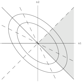
Figure 1: Schematic structure of the energy spectrum. The ellipses correspond to levels of different energies, states with $E=\lambda^{\prime}n^{2}$ ($E=3\lambda^{\prime}n^{2}$) lie on continuous (dashed) lines. The shaded area contains the full information of the spectrum.

The condition (4.4) can now be interpreted as the restriction to the set of states, where $(m_{1},m_{2})$ lies within the ellipse given by $E_{|n_{1},n_{2};1\rangle}$. Although this picture appears to be rather simple, it remains a nontrivial problem to specify the limits of the sums over $m_{1}$ and $m_{2}$ explicitly. However, this problem can be solved at least numerically. The resulting decay widths have been plotted in figure 2 for $n_{1},n_{2}\in[-8,8]$. We will not describe this method in detail and turn instead to the second decay channel, where this problem does not occur.

For the decay channel 2 the condition (4.4) is replaced by $|m|\leq n_{1}^{2}+n_{2}^{2}+n_{1}n_{2}$ and thus (4.1) is given by

$$\Gamma^{(2)}=2\pi\sum_{(a,b)(c)}\sum_{m=-[Q]}^{[Q]}\int_{0}^{1}ds \;\big{|}\;^{\text{\tiny c}}\langle s|\;^{\text{\tiny ab}}\langle m;1-s|\tilde{H}|n_{1},n_{2};1\rangle\big{|}^{2}\;$$

$$\times\delta(E_{|n_{1},n_{2};1\rangle}-E_{|m;1-s\rangle|s\rangle})\;,$$ (4.7)

where $Q\equiv\sqrt{n_{1}^{2}+n_{2}^{2}+n_{1}n_{2}}$ and $[Q]$ denotes the integer part of $Q$. Plugging in the matrix element of $\tilde{H}$ from (2.3) and rewriting the $\delta$-function in the same manner as it was done in (4) leads to

$$\Gamma^{(2)}=\frac{\lambda^{\prime}\,g_{2}^{2}}{4\pi^{5}}\frac{1}{Q^{2}}\,A_{n_{1},n_{2}}\,B_{n_{1},n_{2}}\qquad\text{with}\;$$ (4.8)

$$A_{n_{1},n_{2}}=\sum_{m=1}^{[Q]}\,\sin^{2}\big{(}\pi\,n_{1}\,\frac{m}{Q}\,\big{)}\,\sin^{2}\big{(}\pi\,n_{2}\,\frac{m}{Q}\,\big{)}\,\sin^{2}\big{(}\pi\,(n_{1}+n_{2})\,\frac{m}{Q}\,\big{)}\,,$$

$$B_{n_{1},n_{2}}=\sum_{(a,b)(c)}\Big{\{}\Big{(}\frac{1}{N_{a}+Q}+\frac{1}{N_{b}-Q}+\frac{1}{N_{c}}\Big{)}^{2}+\Big{(}\frac{1}{N_{a}-Q}+\frac{1}{N_{b}+Q}+\frac{1}{N_{c}}\Big{)}^{2}\Big{\}}$$

$$\phantom{B_{n_{1},n_{2}}}=\,18\,\frac{Q^{4}}{n_{1}^{2}\,n_{2}^{2}\,(n_{1}+n_{2})^{2}}$$

after the integration over $s$. The sum $A_{n_{1},n_{2}}$ is calculated in Appendix B. We finally find the result

$$\Gamma^{(2)}=\frac{9\lambda^{\prime}\,g_{2}^{2}}{2\pi^{5}}A^{\prime}_{n_{1},n_{2}}$$ (4.9)

with

$$A^{\prime}_{n_{1},n_{2}}\left\{\begin{aligned} &=0\\ &\quad\;\text{for}\quad n_{1}=n_{2}=0,\,n_{1}=0\wedge n_{2}\neq 0,\,n_{1}\neq 0\wedge n_{2}=0\,,\,n_{1}=-n_{2}\\[8.53581pt] &=\tfrac{1}{32}\,\tfrac{3}{4n^{2}}\,\big{(}\,\tfrac{5}{2}(1+2[Q])-2s_{(1)}(1)-2s_{(1)}(2)+2s_{(1)}(3)-\tfrac{1}{2}s_{(1)}(4)\,\big{)}\\ &\quad\;\text{for}\quad n\equiv n_{1}=n_{2},\,n\equiv n_{1}=-2n_{2}\,,\,n\equiv-2n_{1}=n_{2}\\[8.53581pt] &=\tfrac{1}{32}\tfrac{Q^{2}}{n_{1}^{2}\,n_{2}^{2}\,(n_{1}+n_{2})^{2}}\big{(}\tfrac{3}{2}(1+2[Q])-s_{(2)}(n_{1})-s_{(2)}(n_{2})-s_{(2)}(n_{1}+n_{2})\\ &\qquad\qquad\qquad\quad-\tfrac{1}{2}s_{(2)}(2n_{1})-\tfrac{1}{2}s_{(2)}(2n_{2})-\tfrac{1}{2}s_{(2)}(2(n_{1}+n_{2}))\\ &\qquad\qquad\qquad\quad+s_{(2)}(n_{1}-n_{2})+s_{(2)}(2n_{1}+n_{2})+s_{(2)}(n_{1}+2n_{2})\big{)}\\ &\quad\;\,\text{else,}\end{aligned}\right.$$

where we have defined

$$s_{(1)}(x)=\frac{\sin(\pi\,x\,(1+2[Q])/\sqrt{3})}{\sin(\pi x/\sqrt{3})}\quad\text{and}\quad s_{(2)}(x)=\frac{\sin(\pi\,x\,(1+2[Q])/Q)}{\sin(\pi x/Q)}.$$ (4.10)

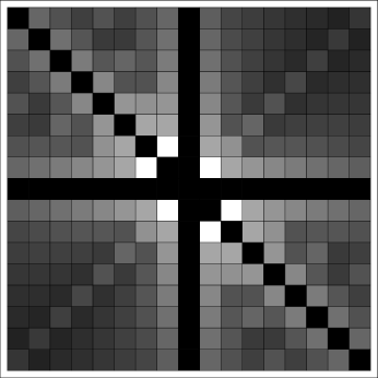
Figure 2: The decay width is plotted against $(n_{1},n_{2})$ (left: decay channel 1 (numerical result), $n_{1},n_{2}\in[-8,8]$; right: decay channel 2, $n_{1},n_{2}\in[-100,100]$), where the relative brightness of the cells is a measure for the relative size of $\Gamma$ (e.g. $\Gamma=0$ corresponds to black cells).

Note that the two classes of symmetry axes reappear in the first two cases of $A_{n_{1},n_{2}}^{\prime}$. In figure 2 the decay width $\Gamma^{(2)}$ is plotted against $n_{1}$ and $n_{2}$. The axes with $E=\lambda^{\prime}n^{2}$ and $E=3\lambda^{\prime}n^{2}$ are highly visible. It is remarkable, that although the range in which $\Gamma^{(1)}$ was computed is comparatively small, one can already recognize the same structures.

Finally, let us note that the decay width (4.1) could have equally well been computed with the (non Hermitian!) gauge theory Hamiltonian $H$, a fact also noted in the two-impurity sector in [14]. To see this, consider the string Hamiltonian matrix element

$$\langle f|\tilde{H}|i\rangle=\langle f|H|i\rangle+\frac{g_{2}}{2}(E_{i}-E_{f})\,\langle f|\Sigma|i\rangle+{\cal O}(g_{2}{}^{2})$$ (4.11)

upon using (2.24). Hence for degenerate states $|i\rangle$ and $|f\rangle$ the discrepancy between matrix elements of $\tilde{H}$ and $H$ vanishes up to order $g_{2}{}^{2}$ – provided there are no poles at degeneracy in $\langle f|\Sigma|i\rangle$, which is not the case. Therefore the decay width $\Gamma$ of (4.1) may also be written as

$$\Gamma=\sum_{f}2\pi\langle i|H|f\rangle\,\langle f|H|i\rangle\,\delta(E_{i}-E_{f})$$ (4.12)

and the knowledge of the $\Sigma$ matrix elements is irrelevant for the computation of this physical quantity.

5 Conclusions

Finally we have a brief look at the 2-loop calculation. In [18] the 2-loop dilatation operator $D_{4}$ was computed. Applied to two-impurity states in the BMN limit $D_{4}$ just acts as the square of $D_{2}$, i.e.

$$\lim_{\stackrel{{\scriptstyle N,J\to\infty,}}{{{}_{N/J^{2}\,\text{fixed}}}}}{\cal D}_{4}\circ{\cal O}_{\rm 2imp}\propto H^{2}\circ{\cal O}_{\rm 2imp}\,.$$ (5.1)

This simple relation does not hold for more than two impurities. Instead, one obtains for three impurities at the planar level

$$({D}_{4})_{\rm planar}|x_{1},x_{2},1-x_{1}-x_{2}\rangle\propto\Big{[}\partial_{x_{1}}^{4}+(\partial_{x_{1}}-\partial_{x_{2}})^{4}+\partial_{x_{2}}^{4}\Big{]}|x_{1},x_{2},1-x_{1}-x_{2}\rangle\;,\$$ (5.2)

which will lead to “energy” eigenvalues $E_{{\mathcal{O}}(\lambda^{\prime 2})}\propto n_{1}^{4}+n_{2}^{4}+(n_{1}+n_{2})^{4}$ not being a perfect square. This result confirms what one would expect from the string theory point of view from expanding out the square root in (1.2).

In this paper we have studied the quantum mechanics of BMN gauge theory in the sector of three scalar impurities. The relevant matrix elements of the Hamiltonian in the gauge and string theory basis were computed and agreement with string field theory was demonstrated. Finally the decay widths of three-impurity single trace states into double trace states were found. It was shown that in the three-impurity sector the instability of single trace states is a first order process.

Our results represent another non-trivial check of the proposed duality of plane wave strings and ${\cal N}=4$ Super Yang-Mills. Despite of this success, a number of worrying disagreements between plane wave string and gauge theory are known: The reported discrepancy in the two-impurity sector at two quantum-loop order ($\lambda^{\prime 2}$) noted in [24] is unresolved, although there only matrix elements in string and gauge theory were compared. A priori these need not agree. It would be highly desirable to compute a physical quantity, such as an energy shift or a decay width at order $\lambda^{\prime}{}^{2}$ in string field theory to see whether this disagreement is really there. A further discrepancy consists in the existence of impurity non-conserving amplitudes in string field theory at order $\sqrt{\lambda^{\prime}}$, which obviously have no counterpart in perturbative Yang-Mills [25]. The number of disagreements grows as one moves away from the plane-wave limit: Incorporating the first curvature corrections to the plane-wave limit of superstring theory yields different corrections to the spectrum than the corresponding $1/J$ corrections on the gauge side, starting at three loop order in the planar sector [26, 20]. Similarly, discrepancies at three loop order appear in the comparisons of gauge theory scaling dimensions and semiclassical spinning string solutions in the full $AdS_{5}\times S^{5}$ theory [27].

It remains to be seen how this miraculous mosaic of perturbative agreements and disagreements of string and gauge theory is to be understood.

Acknowledgments
We would like to thank Niklas Beisert, Dan Freedman and Ari Pankiewicz for interesting discussions. P.G. thanks the University of Washington for hospitality extended to her in the final stages of this project.

Appendix

A.1 Action of the 1-loop vertex operator on ${\mathcal{O}}_{3;l}$, ${\mathcal{O}}_{2,1;l}$ and ${\mathcal{O}}_{1,1,1;l}$

In this Appendix we present the expressions for $H\circ{\mathcal{O}}$ (${\mathcal{O}}$ stands for the three different types of operators we introduced in section 2), which can be obtained by performing Wick contractions. We begin with operators of the type ${\mathcal{O}}_{3;l}$. The trace-conserving part $H_{0}\circ{\mathcal{O}}_{3;l}$ reads

$${\it H}_{0}\circ{\mathcal{O}}^{\text{\tiny 123}}_{p_{1},p_{2},J_{0}-p_{1}-p_{2}}{\mathcal{O}}_{J_{1}}\ldots{\mathcal{O}}_{J_{l}}=$$

$$\>\tfrac{g_{\rm YM}^{2}N}{8\pi^{2}}\Big{[}6{\mathcal{O}}^{\text{\tiny 123}}_{p_{1},p_{2},J_{0}-p_{1}-p_{2}}-{\mathcal{O}}^{\text{\tiny 123}}_{p_{1}-1,p_{2},J_{0}-\left(p_{1}-1\right)-p_{2}}-{\mathcal{O}}^{\text{\tiny 123}}_{p_{1}+1,p_{2},J_{0}-\left(p_{1}+1\right)-p_{2}}$$

$$\quad\quad\quad-{\mathcal{O}}^{\text{\tiny 123}}_{p_{1},p_{2}+1,J_{0}-p_{1}-\left(p_{2}+1\right)}-{\mathcal{O}}^{\text{\tiny 123}}_{p_{1},p_{2}-1,J_{0}-p_{1}-\left(p_{2}-1\right)}$$

$$\quad\quad\quad-{\mathcal{O}}^{\text{\tiny 123}}_{p_{1}+1,p_{2}-1,J_{0}-p_{1}-p_{2}}-{\mathcal{O}}^{\text{\tiny 123}}_{p_{1}-1,p_{2}+1,J_{0}-p_{1}-p_{2}}\Big{]}{\mathcal{O}}_{J_{1}}\ldots{\mathcal{O}}_{J_{l}}\,,\hskip 28.45274pt$$ (A.1)

while $H_{\pm}\circ{\mathcal{O}}_{3;l}$, where the number of traces in- and decreases, are given by

$${\it H}_{+}\circ{\mathcal{O}}^{\text{\tiny 123}}_{p_{1},p_{2},J_{0}-p_{1}-p_{2}}{\mathcal{O}}_{J_{1}}\ldots{\mathcal{O}}_{J_{l}}=$$

$$\>\tfrac{g_{\rm YM}^{2}}{8\pi^{2}}\bigg{\{}\sum_{i=1}^{p_{1}-1}\Big{(}2{\mathcal{O}}^{\text{\tiny 123}}_{p_{1}-i,p_{2},J_{0}-p_{1}-p_{2}}-{\mathcal{O}}^{\text{\tiny 123}}_{p_{1}-i-1,p_{2}+1,J_{0}-p_{1}-p_{2}}$$

$$\qquad\qquad\quad-{\mathcal{O}}^{\text{\tiny 123}}_{p_{1}-i-1,p_{2},J_{0}-\left(p_{1}-1\right)-p_{2}}\Big{)}{\mathcal{O}}_{i}$$

$$\quad\>+\sum_{i=1}^{p_{2}-1}\Big{(}2{\mathcal{O}}^{\text{\tiny 123}}_{p_{1},p_{2}-i,J_{0}-p_{1}-p_{2}}-{\mathcal{O}}^{\text{\tiny 123}}_{p_{1},p_{2}-i-1,J_{0}-p_{1}-\left(p_{2}-1\right)}$$

$$\qquad\qquad\quad-{\mathcal{O}}^{\text{\tiny 123}}_{p_{1}+1,p_{2}-i-1,J_{0}-p_{1}-p_{2}}\Big{)}{\mathcal{O}}_{i}$$

$$\quad\>+\sum_{i=1}^{J_{0}-p_{1}-p_{2}-1}\Big{(}2{\mathcal{O}}^{\text{\tiny 123}}_{p_{1},p_{2},J_{0}-p_{1}-p_{2}-i}-{\mathcal{O}}^{\text{\tiny 123}}_{p_{1}+1,p_{2},J_{0}-\left(p_{1}+1\right)-p_{2}-i}$$

$$\qquad\qquad\quad-{\mathcal{O}}^{\text{\tiny 123}}_{p_{1},p_{2}+1,J_{0}-p_{1}-\left(p_{2}+1\right)-i}\Big{)}{\mathcal{O}}_{i}$$

$$\quad\>+\sum_{i=0}^{p_{1}-1}\Big{(}{\mathcal{O}}^{\text{\tiny 1}}_{J_{0}-p_{1}-p_{2}+i}\Big{[}{\mathcal{O}}^{\text{\tiny 23}}_{p_{2},p_{1}-i}-{\mathcal{O}}^{\text{\tiny 23}}_{p_{2}+1,p_{1}-i-1}\Big{]}$$

$$\qquad\qquad\quad+{\mathcal{O}}^{\text{\tiny 2}}_{p_{2}+i}\Big{[}{\mathcal{O}}^{\text{\tiny 31}}_{J_{0}-p_{1}-p_{2},p_{1}-i}-{\mathcal{O}}^{\text{\tiny 31}}_{J_{0}-\left(p_{1}-1\right)-p_{2},p_{1}-i-1}\Big{]}\Big{)}\hskip 56.9055pt$$

$$\quad\>+\sum_{i=0}^{p_{2}-1}\Big{(}{\mathcal{O}}^{\text{\tiny 2}}_{p_{1}+i}\Big{[}{\mathcal{O}}^{\text{\tiny 31}}_{J_{0}-p_{1}-p_{2},p_{2}-i}-{\mathcal{O}}^{\text{\tiny 31}}_{J_{0}-p_{1}-\left(p_{2}-1\right),p_{2}-i-1}\Big{]}$$

$$\qquad\qquad\quad+{\mathcal{O}}^{\text{\tiny 3}}_{J_{0}-p_{1}-p_{2}+i}\Big{[}{\mathcal{O}}^{\text{\tiny 12}}_{p_{1},p_{2}-i}-{\mathcal{O}}^{\text{\tiny 12}}_{p_{1}+1,p_{2}-i-1}\Big{]}\Big{)}$$

$$\quad\>+\sum_{i=0}^{J_{0}-p_{1}-p_{2}-1}\Big{(}{\mathcal{O}}^{\text{\tiny 3}}_{p_{2}+i}\Big{[}{\mathcal{O}}^{\text{\tiny 12}}_{p_{1},J_{0}-p_{1}-p_{2}-i}-{\mathcal{O}}^{\text{\tiny 12}}_{p_{1}+1,J_{0}-\left(p_{1}+1\right)-p_{2}-i}\Big{]}$$

$$\qquad\qquad\quad+{\mathcal{O}}^{\text{\tiny 1}}_{p_{1}+i}\Big{[}{\mathcal{O}}^{\text{\tiny 23}}_{p_{2},J_{0}-p_{1}-p_{2}-i}-{\mathcal{O}}^{\text{\tiny 23}}_{p_{2}+1,J_{0}-p_{1}-\left(p_{2}+1\right)-i}\Big{]}\Big{)}\bigg{\}}{\mathcal{O}}_{J_{1}}\ldots{\mathcal{O}}_{J_{l}}\hskip 19.91684pt$$ (A.2)

and

$${\it H}_{-}\circ{\mathcal{O}}^{\text{\tiny 123}}_{p_{1},p_{2},J_{0}-p_{1}-p_{2}}{\mathcal{O}}_{J_{1}}\ldots{\mathcal{O}}_{J_{l}}=$$

$$\>\tfrac{g_{\rm YM}^{2}}{8\pi^{2}}\sum_{i=1}^{l}J_{i}\Big{(}2{\mathcal{O}}^{\text{\tiny 123}}_{p_{1}+J_{i},p_{2},J_{0}-p_{1}-p_{2}}-{\mathcal{O}}^{\text{\tiny 123}}_{p_{1}+J_{i}-1,p_{2}+1,J_{0}-p_{1}-p_{2}}$$

$$\qquad\qquad\quad-{\mathcal{O}}^{\text{\tiny 123}}_{p_{1}+J_{i}-1,p_{2},J_{0}-\left(p_{1}-1\right)-p_{2}}$$

$$\qquad\qquad\quad+2{\mathcal{O}}^{\text{\tiny 123}}_{p_{1},p_{2}+J_{i},J_{0}-p_{1}-p_{2}}-{\mathcal{O}}^{\text{\tiny 123}}_{p_{1},p_{2}+J_{i}-1,J_{0}-p_{1}-\left(p_{2}-1\right)}$$

$$\qquad\qquad\quad-{\mathcal{O}}^{\text{\tiny 123}}_{p_{1}+1,p_{2}+J_{i}-1,J_{0}-p_{1}-p_{2}}$$

$$\qquad\qquad\quad+2{\mathcal{O}}^{\text{\tiny 123}}_{p_{1},p_{2},J_{0}-p_{1}-p_{2}+J_{i}}-{\mathcal{O}}^{\text{\tiny 123}}_{p_{1}+1,p_{2},J_{0}-\left(p_{1}+1\right)-p_{2}+J_{i}}$$

$$\qquad\qquad\quad-{\mathcal{O}}^{\text{\tiny 123}}_{p_{1},p_{2}+1,J_{0}-p_{1}-\left(p_{2}+1\right)+J_{i}}\Big{)}\times{\mathcal{O}}_{J_{1}}\ldots\makebox[0.0pt]{$\not$}{\mathcal{O}}_{J_{i}}\ldots{\mathcal{O}}_{J_{l}}\,.\hskip 42.67912pt$$ (A.3)

The same can be done for ${\mathcal{O}}_{2,1;l}$ with

$${\it H}_{0}\circ{\mathcal{O}}^{\text{\tiny ab}}_{p,J_{0}-p-q}{\mathcal{O}}^{\text{\tiny c}}_{q}{\mathcal{O}}_{J_{1}}\ldots{\mathcal{O}}_{J_{l}}=$$

$$\;\tfrac{g_{\rm YM}^{2}N}{4\pi^{2}}\Big{[}2{\mathcal{O}}^{\text{\tiny ab}}_{p,J_{0}-p-q}-{\mathcal{O}}^{\text{\tiny ab}}_{p+1,J_{0}-(p+1)-q}-{\mathcal{O}}^{\text{\tiny ab}}_{p-1,J_{0}-(p-1)-q}\Big{]}{\mathcal{O}}^{\text{\tiny c}}_{q}{\mathcal{O}}_{J_{1}}\ldots{\mathcal{O}}_{J_{l}}\,,$$ (A.4)

$${\it H}_{+}\circ{\mathcal{O}}^{\text{\tiny ab}}_{p,J_{0}-p-q}{\mathcal{O}}^{\text{\tiny c}}_{q}{\mathcal{O}}_{J_{1}}\ldots{\mathcal{O}}_{J_{l}}=$$

$$\;\tfrac{g_{\rm YM}^{2}}{4\pi^{2}}\bigg{[}\sum_{i=1}^{p-1}\Big{(}{\mathcal{O}}^{\text{\tiny ab}}_{p-i,J_{0}-p-q}-{\mathcal{O}}^{\text{\tiny ab}}_{p-1-i,J_{0}-(p-1)-q}\Big{)}{\mathcal{O}}_{i}$$

$$\quad+\sum_{i=1}^{J_{0}-p-q-1}\Big{(}{\mathcal{O}}^{\text{\tiny ab}}_{p,J_{0}-p-q-i}-{\mathcal{O}}^{\text{\tiny ab}}_{p+1,J_{0}-(p+1)-q-i}\Big{)}{\mathcal{O}}_{i}\bigg{]}{\mathcal{O}}^{\text{\tiny c}}_{q}{\mathcal{O}}_{J_{1}}\ldots{\mathcal{O}}_{J_{l}}$$ (A.5)

and

$${\it H}_{-}\circ{\mathcal{O}}^{\text{\tiny ab}}_{p,J_{0}-p-q}{\mathcal{O}}^{\text{\tiny c}}_{q}{\mathcal{O}}_{J_{1}}\ldots{\mathcal{O}}_{J_{l}}=$$

$$\;\tfrac{g_{\rm YM}^{2}}{4\pi^{2}}\bigg{\{}\sum_{i=1}^{l}J_{i}\Big{[}{\mathcal{O}}^{\text{\tiny ab}}_{p+J_{i},J_{0}-p-q}-{\mathcal{O}}^{\text{\tiny ab}}_{p-1+J_{i},J_{0}-(p-1)-q}$$

$$\qquad\qquad\quad+{\mathcal{O}}^{\text{\tiny ab}}_{p,J_{0}-p-q+J_{i}}-{\mathcal{O}}^{\text{\tiny ab}}_{p+1,J_{0}-(p+1)-q+J_{i}}\Big{]}{\mathcal{O}}^{\text{\tiny c}}_{q}{\mathcal{O}}_{J_{1}}\ldots\makebox[0.0pt]{$\not$}{\mathcal{O}}_{J_{i}}\ldots{\mathcal{O}}_{J_{l}}$$

$$\quad+\tfrac{1}{2}\bigg{[}\sum_{i=0}^{p-1}\Big{(}{\mathcal{O}}^{\text{\tiny acb}}_{q+i,p-i,J_{0}-p-q}-{\mathcal{O}}^{\text{\tiny acb}}_{q+1+i,p-1-i,J_{0}-p-q}$$

$$\qquad\qquad\quad+{\mathcal{O}}^{\text{\tiny acb}}_{p-i,q+i,J_{0}-p-q}-{\mathcal{O}}^{\text{\tiny acb}}_{p-1-i,q+1+i,J_{0}-p-q}\Big{)}$$

$$\qquad\;+\sum_{i=0}^{J_{0}-p-q-1}\Big{(}{\mathcal{O}}^{\text{\tiny abc}}_{p,q+i,J_{0}-p-q-i}-{\mathcal{O}}^{\text{\tiny abc}}_{p,q+1+i,J_{0}-p-(q+1)-i}$$

$$\qquad\qquad\quad+{\mathcal{O}}^{\text{\tiny abc}}_{p,J_{0}-p-q-i,q+i}-{\mathcal{O}}^{\text{\tiny abc}}_{p,J_{0}-p-(q+1)-i,q+1+i}\Big{)}$$

$$\qquad\;+\sum_{i=0}^{q-1}\Big{(}{\mathcal{O}}^{\text{\tiny abc}}_{p,q-i,J_{0}-p-q+i}-{\mathcal{O}}^{\text{\tiny abc}}_{p+1,q-1-i,J_{0}-p-q+i}$$

$$\qquad\qquad\quad+{\mathcal{O}}^{\text{\tiny abc}}_{p,J_{0}-p-q+i,q-i}-{\mathcal{O}}^{\text{\tiny abc}}_{p+1,J_{0}-p-q+i,q-1-i}$$

$$\qquad\qquad\quad+{\mathcal{O}}^{\text{\tiny acb}}_{q-i,p+i,J_{0}-p-q}-{\mathcal{O}}^{\text{\tiny acb}}_{q-1-i,p+i,J_{0}-p-(q-1)}$$

$$\qquad\qquad\quad+{\mathcal{O}}^{\text{\tiny acb}}_{p+i,q-i,J_{0}-p-q}-{\mathcal{O}}^{\text{\tiny acb}}_{p+i,q-1-i,J_{0}-p-(q-1)}\Big{)}\bigg{]}{\mathcal{O}}_{J_{1}}\ldots{\mathcal{O}}_{J_{l}}\bigg{\}}\,.\hskip 5.69046pt$$ (A.6)

The only non-vanishing contribution of $H\circ{\mathcal{O}}_{1,1,1;l}$ is

$${\it H}_{-}\circ{\mathcal{O}}^{\text{\tiny 1}}_{p_{1}}{\mathcal{O}}^{\text{\tiny 2}}_{p_{2}}{\mathcal{O}}^{\text{\tiny 3}}_{J_{0}-p_{1}-p_{2}}{\mathcal{O}}_{J_{1}}\ldots{\mathcal{O}}_{J_{l}}=$$

$$\;\tfrac{g_{\rm YM}^{2}}{8\pi^{2}}\bigg{[}\sum_{i=0}^{p_{1}-1}\Big{(}\Big{[}{\mathcal{O}}^{\text{\tiny 12}}_{p_{2}+i,p_{1}-i}-{\mathcal{O}}^{\text{\tiny 12}}_{p_{2}+1+i,p_{1}-1-i}$$

$$\qquad\qquad\quad+{\mathcal{O}}^{\text{\tiny 12}}_{p_{1}-i,p_{2}+i}-{\mathcal{O}}^{\text{\tiny 12}}_{p_{1}-1-i,p_{2}+1+i}\Big{]}{\mathcal{O}}^{\text{\tiny 3}}_{J_{0}-p_{1}-p_{2}}$$

$$\qquad\qquad+\Big{[}{\mathcal{O}}^{\text{\tiny 13}}_{J_{0}-p_{1}-p_{2}+i,p_{1}-i}-{\mathcal{O}}^{\text{\tiny 13}}_{J_{0}-(p_{1}-1)-p_{2}+i,p_{1}-1-i}$$

$$\qquad\qquad\quad+{\mathcal{O}}^{\text{\tiny 13}}_{p_{1}-i,J_{0}-p_{1}-p_{2}+i}-{\mathcal{O}}^{\text{\tiny 13}}_{p_{1}-1-i,J_{0}-(p_{1}-1)-p_{2}+i}\Big{]}{\mathcal{O}}^{\text{\tiny 2}}_{p_{2}}\Big{)}\hskip 56.9055pt$$

$$\quad\;+\sum_{i=0}^{p_{2}-1}\Big{(}\Big{[}{\mathcal{O}}^{\text{\tiny 12}}_{p_{2}-i,p_{1}+i}-{\mathcal{O}}^{\text{\tiny 12}}_{p_{2}-1-i,p_{1}+1+i}$$

$$\qquad\qquad\quad+{\mathcal{O}}^{\text{\tiny 12}}_{p_{1}+i,p_{2}-i}-{\mathcal{O}}^{\text{\tiny 12}}_{p_{1}+1+i,p_{2}-1-i}\Big{]}{\mathcal{O}}^{\text{\tiny 3}}_{J_{0}-p_{1}-p_{2}}$$

$$\qquad\qquad+\Big{[}{\mathcal{O}}^{\text{\tiny 23}}_{J_{0}-p_{1}-p_{2}+i,p_{2}-i}-{\mathcal{O}}^{\text{\tiny 23}}_{J_{0}-p_{1}-(p_{2}-1)+i,p_{2}-1-i}$$

$$\qquad\qquad\quad+{\mathcal{O}}^{\text{\tiny 23}}_{p_{2}-i,J_{0}-p_{1}-p_{2}+i}-{\mathcal{O}}^{\text{\tiny 23}}_{p_{2}-1-i,J_{0}-p_{1}-(p_{2}-1)+i}\Big{]}{\mathcal{O}}^{\text{\tiny 1}}_{p_{1}}\Big{)}$$

$$\quad\;+\sum_{i=0}^{J_{0}-p_{1}-p_{2}-1}\Big{(}\Big{[}{\mathcal{O}}^{\text{\tiny 13}}_{J_{0}-p_{1}-p_{2}-i,p_{1}+i}-{\mathcal{O}}^{\text{\tiny 13}}_{J_{0}-(p_{1}+1)-p_{2}-i,p_{1}+1+i}$$

$$\qquad\qquad\quad+{\mathcal{O}}^{\text{\tiny 13}}_{p_{1}+i,J_{0}-p_{1}-p_{2}-i}-{\mathcal{O}}^{\text{\tiny 13}}_{p_{1}+1+i,J_{0}-(p_{1}+1)-p_{2}-i}\Big{]}{\mathcal{O}}^{\text{\tiny 2}}_{p_{2}}$$

$$\qquad\qquad+\Big{[}{\mathcal{O}}^{\text{\tiny 23}}_{J_{0}-p_{1}-p_{2}-i,p_{2}+i}-{\mathcal{O}}^{\text{\tiny 23}}_{J_{0}-p_{1}-(p_{2}+1)-i,p_{2}+1+i}$$

$$\qquad\qquad\quad+{\mathcal{O}}^{\text{\tiny 23}}_{p_{2}+i,J_{0}-p_{1}-p_{2}-i}-{\mathcal{O}}^{\text{\tiny 23}}_{p_{2}+1+i,J_{0}-p_{1}-(p_{2}+1)-i}\Big{]}{\mathcal{O}}^{\text{\tiny 1}}_{p_{1}}\Big{)}\bigg{]}{\mathcal{O}}_{J_{1}}\ldots{\mathcal{O}}_{J_{l}}$$ (A.7)

A.2 ${H}_{-}$ and $\Sigma_{-}$

Here we summarize the action of $H_{-}$ and $\Sigma_{-}$ on the different types of continuum states. The action of $H_{-}$ can be deduced out of the corresponding expressions of Appendix A.1 by taking $J\to\infty$. One gets

$${\it{H}}_{-}|n_{1},n_{2};r_{0}\rangle|r_{1}\rangle\ldots|r_{l}\rangle=$$

$$\;\frac{\lambda^{\prime}}{2\pi^{3}}\sum_{i=1}^{l}\sum_{m_{1},m_{2}}\bigg{(}\frac{\sqrt{r_{i}}}{r_{0}}\sin(\pi m_{1}\tfrac{r_{0}}{r_{0}+r_{i}})\sin(\pi m_{2}\tfrac{r_{0}}{r_{0}+r_{i}})\sin(\pi(m_{1}+m_{2})\tfrac{r_{0}}{r_{0}+r_{i}})$$

$$\qquad\times\bigg{[}\frac{n_{1}(-m_{1}-2m_{2})}{m_{1}-n_{1}\tfrac{r_{0}+r_{i}}{r_{0}}}+\frac{n_{2}(2m_{1}+m_{2})}{m_{2}-n_{2}\tfrac{r_{0}+r_{i}}{r_{0}}}+\frac{-(n_{1}+n_{2})(m_{2}-m_{1})}{-(m_{1}+m_{2})+(n_{1}+n_{2})\tfrac{r_{0}+r_{i}}{r_{0}}}\bigg{]}$$

$$\qquad\times\frac{1}{m_{1}n_{2}-m_{2}n_{1}}\bigg{)}\;|m_{1},m_{2};r_{0}+r_{i}\rangle|r_{1}\rangle\ldots\makebox[0.0pt]{\;\;$\not$}|r_{i}\rangle\ldots|r_{l}\rangle$$ (A.8)

and

$${\it{H}}_{-}|n;r_{0}-s\rangle^{\text{\tiny ab}}|s\rangle^{\text{\tiny c}}|r_{1}\rangle\ldots|r_{l}\rangle=$$

$$\;\frac{\lambda^{\prime}}{\pi^{2}}\bigg{(}\sum_{i=1}^{l}\sum_{m}\sqrt{\frac{r_{i}}{(r_{0}-s+r_{i})(r_{0}-s)}}$$

$$\qquad\quad\times\frac{m\sin^{2}(\pi m\frac{r_{0}-s}{r_{0}-s+r_{i}})}{m-n\tfrac{r_{0}-s+r_{i}}{r_{0}-s}}\;|m;r_{0}-s+r_{i}\rangle^{\text{\tiny ab}}|s\rangle^{\text{\tiny c}}|r_{1}\rangle\ldots\makebox[0.0pt]{\;\;$\not$}|r_{i}\rangle\ldots|r_{l}\rangle$$

$$\quad+\frac{1}{2}\sum_{m_{1},m_{2}}\frac{\sqrt{r_{0}-s}}{r_{0}\,\pi}\sin(\pi m_{1}\tfrac{s}{r_{0}})\sin(\pi m_{2}\tfrac{s}{r_{0}})\sin(\pi(m_{1}+m_{2})\tfrac{s}{r_{0}})$$

$$\qquad\quad\times\sum_{(a,b)(c)}\frac{1}{M_{c}}\Big{(}\frac{M_{c}-M_{b}}{n+M_{a}\tfrac{r_{0}-s}{r_{0}}}-\frac{M_{c}-M_{a}}{n-M_{b}\tfrac{r_{0}-s}{r_{0}}}\Big{)}|m_{1},m_{2};r_{0}\rangle|r_{1}\rangle\ldots|r_{l}\rangle\bigg{)}\hskip 56.9055pt$$ (A.9)

as well as

$${\it{H}}_{-}|t_{1}\rangle^{\text{\tiny 1}}|t_{2}\rangle^{\text{\tiny 2}}|t_{3}\rangle^{\text{\tiny 3}}|r_{1}\rangle\ldots|r_{l}\rangle=$$

$$\;-\frac{\lambda^{\prime}}{\pi^{2}}\sum_{m}\sum_{(a,b)(c)}\frac{\sin^{2}(\pi m\tfrac{t_{a}}{t_{a}+t_{b}})}{\sqrt{t_{a}+t_{b}}}\;|m;t_{a}+t_{b}\rangle^{\text{\tiny ab}}|t_{c}\rangle^{\text{\tiny c}}|r_{1}\rangle\ldots|r_{l}\rangle\,.\hskip 42.67912pt$$ (A.10)

On the other hand, the matrix elements of $\Sigma_{-}$ can be read off from the corresponding two-point functions, where again $J$ is taken to infinity. Then we obtain for the action on states like $|n_{1},n_{2};r_{0}\rangle\ldots$

$$\Sigma_{-}|n_{1},n_{2};r_{0}\rangle|r_{1}\rangle\ldots|r_{l}\rangle$$

$$\>=-\sum_{i=1}^{l}\sum_{m_{1},m_{2}}\frac{\sin(\pi m_{1}\tfrac{r_{0}}{r_{0}+r_{i}})\,\sin(\pi m_{2}\tfrac{r_{0}}{r_{0}+r_{i}})\,\sin(\pi\left(m_{1}+m_{2}\right)\tfrac{r_{0}}{r_{0}+r_{i}})}{(m_{1}-n_{1}\tfrac{r_{0}+r_{i}}{r_{0}})(m_{2}-n_{2}\tfrac{r_{0}+r_{i}}{r_{0}})(-(m_{1}+m_{2})+(n_{1}+n_{2})\tfrac{r_{0}+r_{i}}{r_{0}})}$$

$$\quad\quad\quad\quad\times\frac{\left(r_{0}+r_{i}\right)^{2}\sqrt{r}_{i}}{r_{0}\pi^{3}}\;|m_{1},m_{2};r_{0}+r_{i}\rangle|r_{1}\rangle\ldots\makebox[0.0pt]{\;\;$\not$}|r_{i}\rangle\ldots|r_{l}\rangle$$

$$\quad+\frac{1}{2}\sum_{\begin{subarray}{c}i,j=0\\ i\neq j\end{subarray}}^{l}\sqrt{r_{i}r_{j}(r_{i}+r_{j})}\;|n_{1},n_{2};r_{0}\rangle|r_{1}\rangle\ldots\makebox[0.0pt]{\;\;$\not$}|r_{i}\rangle\ldots\makebox[0.0pt]{\;\;$\not$}|r_{j}\rangle\ldots|r_{l}\rangle|r_{i}+r_{j}\rangle\,,$$ (A.11)

for states like $|n;r_{0}-s\rangle^{\text{\tiny ab}}|s\rangle^{\text{\tiny c}}\ldots$

$$\Sigma_{-}|n;r_{0}-s\rangle^{\text{\tiny ab}}|s\rangle^{\text{\tiny c}}|r_{1}\rangle\ldots|r_{l}\rangle$$

$$\>=\sum_{i=1}^{l}\Big{(}\sum_{m}\sqrt{\frac{r_{i}(r_{0}-s+r_{i})^{3}}{r_{0}-s}}\frac{\sin^{2}(\pi m\tfrac{r_{0}-s}{r_{0}-s+r_{i}})}{\pi^{2}(m-n\tfrac{r_{0}-s+r_{i}}{r_{0}-s})^{2}}\;|m;r_{0}-s+r_{i}\rangle^{\text{\tiny ab}}|s\rangle^{\text{\tiny c}}$$

$$\quad\quad\quad\quad+\sqrt{r_{i}}\;s\;|n;r_{0}-s\rangle^{\text{\tiny ab}}|s+r_{i}\rangle^{\text{\tiny c}}\Big{)}|r_{1}\rangle\ldots\makebox[0.0pt]{\;\;$\not$}|r_{i}\rangle\ldots|r_{l}\rangle$$

$$\quad+\frac{1}{2}\sum_{\begin{subarray}{c}i,j=0\\ i\neq j\end{subarray}}^{l}\;\sqrt{r_{i}r_{j}(r_{i}+r_{j})}\;|n;r_{0}-s\rangle^{\text{\tiny ab}}|s\rangle^{\text{\tiny c}}|r_{1}\rangle\ldots\makebox[0.0pt]{\;\;$\not$}|r_{i}\rangle\ldots\makebox[0.0pt]{\;\;$\not$}|r_{j}\rangle\ldots|r_{l}\rangle|r_{i}+r_{j}\rangle$$

$$\quad-\sum_{m_{1},m_{2}}\frac{r_{0}^{2}}{\pi^{3}(r_{0}-s)^{1/2}}\;\sin(\pi m_{1}\tfrac{s}{r_{0}})\sin(\pi m_{2}\tfrac{s}{r_{0}})\sin(\pi\left(m_{1}+m_{2}\right)\tfrac{s}{r_{0}})$$

$$\quad\quad\quad\times\left(\left(M_{a}+n\tfrac{r_{0}}{r_{0}-s}\right)\left(M_{b}-n\tfrac{r_{0}}{r_{0}-s}\right)M_{c}\right)^{-1}\;|m_{1},m_{2};r_{0}\rangle|r_{1}\rangle\ldots|r_{l}\rangle$$ (A.12)

and finally for states like $|t_{1}\rangle^{\text{\tiny 1}}|t_{2}\rangle^{\text{\tiny 2}}|t_{3}\rangle^{\text{\tiny 3}}\ldots$

$$\Sigma_{-}|t_{1}\rangle^{\text{\tiny 1}}|t_{2}\rangle^{\text{\tiny 2}}|t_{3}\rangle^{\text{\tiny 3}}|r_{1}\rangle\ldots|r_{l}\rangle$$

$$\;=\sum_{i=1}^{l}\sqrt{r_{i}}\;\Big{(}t_{1}\;|t_{1}+r_{i}\rangle^{\text{\tiny 1}}|t_{2}\rangle^{\text{\tiny 2}}|t_{3}\rangle^{\text{\tiny 3}}+t_{2}\;|t_{1}\rangle^{\text{\tiny 1}}|t_{2}+r_{i}\rangle^{\text{\tiny 2}}|t_{3}\rangle^{\text{\tiny 3}}$$

$$\qquad\qquad+t_{3}\;|t_{1}\rangle^{\text{\tiny 1}}|t_{2}\rangle^{\text{\tiny 2}}|t_{3}+r_{i}\rangle^{\text{\tiny 3}}\Big{)}|r_{1}\rangle...\makebox[0.0pt]{\;\;$\not$}|r_{i}\rangle...|r_{l}\rangle$$

$$\quad+\frac{1}{2}\sum_{\begin{subarray}{c}i,j=0\\ i\neq j\end{subarray}}^{l}\;\sqrt{r_{i}r_{j}(r_{i}+r_{j})}\;|t_{1}\rangle^{\text{\tiny 1}}|t_{2}\rangle^{\text{\tiny 2}}|t_{3}\rangle^{\text{\tiny 3}}|r_{1}\rangle\ldots\makebox[0.0pt]{\;\;$\not$}|r_{i}\rangle\ldots\makebox[0.0pt]{\;\;$\not$}|r_{j}\rangle\ldots|r_{l}\rangle|r_{i}+r_{j}\rangle$$

$$\quad-\sum_{m}\sum_{(a,b)(c)}\frac{(t_{a}+t_{b})^{3/2}}{m^{2}\;\pi^{2}}\;\sin^{2}(\pi m\tfrac{t_{a}}{t_{a}+t_{b}})\;|m;t_{a}+t_{b}\rangle^{\text{\tiny ab}}|t_{c}\rangle^{\text{\tiny c}}|r_{1}\rangle\ldots|r_{l}\rangle\,,$$ (A.13)

with $t_{1}+t_{2}+t_{3}=r_{0}$ and $M_{1}:=-(m_{1}+m_{2})$, $M_{2}:=m_{1}$, $M_{3}:=m_{2}$.

Appendix B The sum $A_{n_{1},n_{2}}$

In the following we will use the short cuts

$$p\equiv\frac{\pi\,n_{1}}{Q}\quad\text{and}\quad q\equiv\frac{\pi\,n_{2}}{Q}\,.$$ (B.1)

The sum $A_{n_{1},n_{2}}$ then reads

$$A_{p,q}=\sum_{m=1}^{[Q]}\,\sin^{2}(p\,m)\,\sin^{2}(q\,m)\,\sin^{2}((p+q)\,m)$$ (B.2)

$$\qquad=\tfrac{1}{32}\sum_{m=1}^{[Q]}\,\big{(}3-2\cos(2\,p\,m)-2\cos(2\,q\,m)-2\cos(2\,(p+q)\,m)$$

$$\qquad\qquad\quad\>-\;\cos(4\,p\,m)-\;\cos(4\,q\,m)-\;\cos(4\,(p+q)\,m)$$

$$\qquad\qquad\quad\>+2\cos(2\,(p-q)\,m)+2\cos(2\,(2p+q)\,m)+2\cos(2\,(p+2q)\,m)\big{)}.$$

Before calculating the sum we study the cases, where at least one of the arguments of the cosines vanishes, namely

• $p=q=0$, $p=0\wedge q\neq 0$, $p\neq 0\wedge q=0$ and $p=-q$   :   $\Gamma^{(2)}\rightarrow 0$

• $r\equiv p=q$, $r\equiv p=-2q$ and $r\equiv-2p=q$  :
  $\quad A_{p,q}\rightarrow A_{r}=\tfrac{1}{32}\sum_{m=1}^{[Q]}\big{(}5-4\cos(2\,r\,m)-4\cos(4\,r\,m)+4\cos(6\,r\,m)-\cos(8\,r\,m)\big{)}$ .

Using

$$\sum_{m=1}^{[Q]}\cos(x\,m)=-1+\cos(\tfrac{[Q]\,x}{2})\csc(\tfrac{x}{2})\sin(\tfrac{x}{2}(1+[Q]))\quad\text{for}\quad\frac{x}{2\pi}\not\in\mathbb{Z}$$

$A_{n_{1},n_{2}}$ as stated in (4.9) and (4.10) follows.

References

• [1] D. Berenstein, J. M. Maldacena and H. Nastase, “Strings in flat space and pp waves from N = 4 super Yang Mills,” JHEP 0204 (2002) 013, [hep-th/0202021].
• [2] A. Pankiewicz, “Strings in plane wave backgrounds,” Fortsch. Phys.  51 (2003) 1139 [hep-th/0307027]. $\bullet$  J. C. Plefka, “Lectures on the plane-wave string / gauge theory duality,” Fortsch. Phys.  52 (2004) 264 [hep-th/0307101]. $\bullet$  C. Kristjansen, “Quantum mechanics, random matrices and BMN gauge theory,” Acta Phys. Polon. B 34 (2003) 4949 [hep-th/0307204]. $\bullet$  M. Spradlin and A. Volovich, “Light-cone string field theory in a plane wave,” [hep-th/0310033]. $\bullet$  D. Sadri and M. M. Sheikh-Jabbari, “The plane-wave / super Yang-Mills duality,” [hep-th/0310119]. $\bullet$  R. Russo and A. Tanzini, “The duality between IIB string theory on pp-wave and N = 4 SYM: A status report,” [hep-th/0401155].
• [3] J. M. Maldacena, “The large N limit of superconformal field theories and supergravity,” Adv. Theor. Math. Phys.  2 (1998) 231 [Int. J. Theor. Phys.  38 (1999) 1113], [hep-th/9711200].
• [4] M. Blau, J. Figueroa-O’Farrill, C. Hull and G. Papadopoulos, “A new maximally supersymmetric background of IIB superstring theory,” JHEP 0201 (2002) 047 [hep-th/0110242].
• [5] C. Kristjansen, J. Plefka, G. W. Semenoff and M. Staudacher, “A new double-scaling limit of N = 4 super Yang-Mills theory and PP-wave strings,” Nucl. Phys. B 643 (2002) 3, [hep-th/0205033].
• [6] N. R. Constable, D. Z. Freedman, M. Headrick, S. Minwalla, L. Motl, A. Postnikov and W. Skiba, “PP-wave string interactions from perturbative Yang-Mills theory,” JHEP 0207 (2002) 017, [hep-th/0205089].
• [7] R. R. Metsaev, “Type IIB Green-Schwarz superstring in plane wave Ramond-Ramond background,” Nucl. Phys. B 625 (2002) 70, [hep-th/0112044]. $\bullet$  R. R. Metsaev and A. A. Tseytlin, “Exactly solvable model of superstring in plane wave Ramond-Ramond background,” Phys. Rev. D 65, 126004 (2002), [hep-th/0202109].
• [8] M. Spradlin and A. Volovich, “Superstring interactions in a pp-wave background,” Phys. Rev. D 66 (2002) 086004, [hep-th/0204146]. $\bullet$  M. Spradlin and A. Volovich, “Superstring interactions in a pp-wave background. II,” JHEP 0301 (2003) 036, [hep-th/0206073]. $\bullet$  J. H. Schwarz, “Comments on superstring interactions in a plane-wave background,” JHEP 0209 (2002) 058 [arXiv:hep-th/0208179]. $\bullet$  A. Pankiewicz, “More comments on superstring interactions in the pp-wave background,” JHEP 0209 (2002) 056 [arXiv:hep-th/0208209]. $\bullet$  A. Pankiewicz and B. Stefanski, “pp-wave light-cone superstring field theory,” Nucl. Phys. B 657 (2003) 79, [hep-th/0210246]. $\bullet$  P. Di Vecchia, J. L. Petersen, M. Petrini, R. Russo and A. Tanzini, “The 3-string vertex and the AdS/CFT duality in the pp-wave limit,” [hep-th/0304025].
• [9] D. J. Gross, A. Mikhailov and R. Roiban, “A calculation of the plane wave string Hamiltonian from N = 4 super-Yang-Mills theory,” JHEP 0305 (2003) 025, [hep-th/0208231]. $\bullet$  J. Gomis, S. Moriyama and J. w. Park, “SYM description of SFT Hamiltonian in a pp-wave background,” Nucl. Phys. B 659 (2003) 179, [hep-th/0210153].
• [10] N. Beisert, C. Kristjansen, J. Plefka, G. W. Semenoff and M. Staudacher, “BMN correlators and operator mixing in N = 4 super Yang-Mills theory,” Nucl. Phys. B 650 (2003) 125, [hep-th/0208178]. $\bullet$  N. R. Constable, D. Z. Freedman, M. Headrick and S. Minwalla, “Operator mixing and the BMN correspondence,” JHEP 0210, 068 (2002), [hep-th/0209002].
• [11] N. Beisert, C. Kristjansen, J. Plefka and M. Staudacher, “BMN gauge theory as a quantum mechanical system,” Phys. Lett. B 558 (2003) 229, [hep-th/0212269].
• [12] G. Georgiou and V. V. Khoze, “BMN operators with three scalar impurites and the vertex-correlator duality in pp-wave,” JHEP 0304 (2003) 015, [hep-th/0302064].
• [13] J. Gomis, S. Moriyama and J. w. Park, “SYM description of pp-wave string interactions: Singlet sector and arbitrary impurities,” Nucl. Phys. B 665 (2003) 49, [hep-th/0301250].
• [14] D. Z. Freedman and U. Gursoy, “Instability and degeneracy in the BMN correspondence,” JHEP 0308 (2003) 027, [hep-th/0305016].
• [15] P. Bonderson, “Decay modes of unstable strings in plane-wave string field theory,” [hep-th/0307033].
• [16] G. D’Appollonio and E. Kiritsis, “String interactions in gravitational wave backgrounds,” Nucl. Phys. B 674 (2003) 80 [hep-th/0305081].
• [17] R. A. Janik, “BMN operators and string field theory,” Phys. Lett. B 549 (2002) 237, [hep-th/0209263].
• [18] N. Beisert, C. Kristjansen and M. Staudacher, “The dilatation operator of N = 4 super Yang-Mills theory,” Nucl. Phys. B 664 (2003) 131, [hep-th/0303060].
• [19] N. Beisert, “The complete one-loop dilatation operator of N = 4 super Yang-Mills theory,” Nucl. Phys. B 676 (2004) 3, [hep-th/0307015].
• [20] N. Beisert, “The su(2$|$3) dynamic spin chain,” [hep-th/0310252]. $\bullet$  T. Klose and J. Plefka, “On the integrability of large N plane-wave matrix theory,” Nucl. Phys. B 679 (2004) 127 [hep-th/0310232].
• [21] Y. H. He, J. H. Schwarz, M. Spradlin and A. Volovich, “Explicit formulas for Neumann coefficients in the plane-wave geometry,” Phys. Rev. D 67 (2003) 086005, [hep-th/0211198].
• [22] J. Lucietti, S. Schafer-Nameki and A. Sinha, “On the plane-wave cubic vertex,” [hep-th/0402185].
• [23] D. Vaman and H. Verlinde, “Bit strings from N = 4 gauge theory,” JHEP 0311 (2003) 041, [hep-th/0209215].
• [24] M. Spradlin and A. Volovich, “Note on plane wave quantum mechanics,” Phys. Lett. B 565 (2003) 253, [hep-th/0303220].
• [25] I. R. Klebanov, M. Spradlin and A. Volovich, “New effects in gauge theory from pp-wave superstrings,” Phys. Lett. B 548 (2002) 111, [hep-th/0206221].
• [26] C. G. . Callan, H. K. Lee, T. McLoughlin, J. H. Schwarz, I. Swanson and X. Wu, “Quantizing string theory in AdS(5) x S**5: Beyond the pp-wave,” Nucl. Phys. B 673 (2003) 3, [hep-th/0307032].
• [27] J. A. Minahan and K. Zarembo, “The Bethe-ansatz for N = 4 super Yang-Mills,” JHEP 0303 (2003) 013 [hep-th/0212208]. $\bullet$  S. Frolov and A. A. Tseytlin, “Rotating string solutions: AdS/CFT duality in non-supersymmetric sectors,” Phys. Lett. B 570 (2003) 96, [hep-th/0306143]. $\bullet$  D. Serban and M. Staudacher, “Planar N = 4 gauge theory and the Inozemtsev long range spin chain,” [hep-th/0401057].