Non summable Borel $\Phi^{4}$ theory in zero dimensions and the Generalized Borel Transform

A new technique named Generalized Borel Transform (GBT) is applied to the generating functional of the $\Phi^{4}$ theory in zero dimensions with degenerate minima. The analytical solution of this function, obtained in the non perturbative regime, is compared with those estimations predicted by large order perturbation theory. It was established that the GBT is a very efficient technique to capture these contributions. On the other hand, renormalons associated to the resummation of those perturbative series were not found to be the genuine source of the non perturbative contributions of this model.

Keywords: Non perturbative technique, Borel transform.
PACS numbers: 11.15Tk, 02.30Mv.

Substantial improvement of experimental data has recently demanded theorists to give more accurate estimates since the finite order perturbative predictions have uncertainties comparable with experimental errors. This has renewed the interest in computing non perturbative contributions from the resummation of series. In Quantum Field theory non summable Borel, the problem of obtaining these contributions has been largely studied in the literature.¹ Among the different methods proposed to tackle this problem, the Conventional Borel Transform (CBT) of the weak coupling expansion² and its modified version (MBT)^3,4 have become popular tools for the reconstruction of the physical quantities predicted by these theories. Basically, these techniques require the exact knowledge of the large order behavior of the perturbative series in the coupling parameter. In spite of the lack of these series, which are divergent,⁵ one can make use of their coefficients to define other expansion in powers of a new variable named Borel and in such a way that it is convergent. Then, the resummation of the initial asymptotic series is formally recovered by integrating the convergent series on the Borel variable. In this approach, the non perturbative contributions are estimated from the ambiguity appearing in the integration, where singularities (poles and/or branches) called IR renormalons⁶ localized on the positive real semiaxis of the Borel complex plane invalidate these proposals. On the other hand, an alternative development, called the Generalized Borel Transform (GBT),^7-9 was recently presented which has proved to be potentially useful in overcoming those difficulties. It avoids the use of series by introducing auxiliary parameters having no physical meaning which are introduced for the sole purpose of making the calculation analytically tractable. These parameters together with the analytic properties of the GBT are the fundamental tools needed to obtain analytical solutions of parametric integrals like Laplace-Fourier-Mellin transforms (LFMT) for all the range of its parameter. Therefore, it is extremely useful to study non-perturbative regimes. In addition, it involves simple mathematics which requires basic calculus such as the evaluation of derivative, indefinite integrals and limits. In fact, this technique has already been successfully applied to different areas of Physics such as Quantum Field Theory,⁷ Polymer Physics⁸ and Quantum Mechanics.⁹

In connection with the techniques previously mentioned, it is certainly instructive to study exactly solvable models so that the efficiency and precision of the different proposals can be quantitatively checked. This analysis may help in defining criteria for selecting the appropriate approach to be used in more realistic models. In this sense, it is largely accepted that the analysis of zero-dimensional models can provide some insight on the behavior of Green’s functions in Field theories and Statistical systems.¹⁰ In particular, the understanding of some aspects of zero-dimensional Field Theories could leave trails about the non perturbative behavior of these theories in higher dimensions. For instance, classical actions with degenerate isolated minima play a fundamental role in studying processes governing the decay of metastable atomic and nuclear states as well as the transition of overheated or undercooled thermodynamic phases to a stable equilibrium phase.

One of the most popular model of this kind is the well-known zero-dimensional $\Phi^{4}$ theory with a degenerate minima¹ due to its purely non perturbative feature. The analysis of this model is often based on the study of its generating function, starting point for computing moments and Green’s functions. Moreover, at present the exact solution is known from the numerical computation of its integral representation

$$Z\left(g\right)=\int_{-\infty}^{+\infty}dx\exp\left[-x^{2}\left(1-gx\right)^{2}/2\right],\qquad g\geq 0.$$ (1)

Therefore, the main purpose of this paper consists in discussing the use and to remark the advantages of the different approximate computing tools aforementioned to obtain an analytical approximate solution of the generating function (1) in the non perturbative regime.

Thus, the analysis of this model is initially done on the context of Perturbative Field Theory in which non perturbative contributions are estimated from the solution of the generating functional (1) in powers of $g.$ It is easily obtained by rewriting the integrand in Eq.(1) as a product of two exponential functions as follows

$$Z\left(g\right)=\int_{-\infty}^{+\infty}dx\exp\left[-x^{2}/2\right]\exp\left[gx^{3}-g^{2}x^{4}/2\right].$$

Then, the expansion of the second exponential in powers of its argument leads to the following formal solution of this model

$$Z_{P}\left(g\right)=\sqrt{2\pi}+\sqrt{2}\sum_{n=0}^{\infty}\frac{\Gamma\left(2n+5/2\right)}{\Gamma\left(n+2\right)}\left(8g^{2}\right)^{n+1},\quad g\rightarrow 0^{+}.$$ (2)

Even though this solution is exact, it is plagued of difficulties and consequently it does not represent a suitable analytical solution. Indeed, the series (2) is asymptotic and factorial divergent. Basically, it means that the contributions of the terms of the series decrease with increasing $n$ for $n<n_{min}$ and increase for $n>n_{min}$. The value of $n_{min}=N_{o}\left(g\right)$ corresponds to the term with the minimal contribution to the series. Thus, the best approximation provided by expression (2) is obtained by truncating the series at $n_{min}$. Given that it depends on the value of the parameter $g$, then the accuracy of the result will also depend on it. For example, small values of $g$ provide a large $N_{o}\left(g\right)$ and consequently there are sufficient amounts of terms contained in this series so that a good approximation of the exact solution is obtained. In contrast to this, values of the parameter $g$ going away from the perturbative regime reduce the value of $N_{o}\left(g\right)$ and the series involves just a few terms. Thus, it is significantly off from the exact one. In addition to this trouble, their coefficients do not alternate in sign avoiding the cancelation of the consecutive terms in the series, which makes it worse the divergent behavior.

In some cases, the aforementioned difficulties can be minimized, or hopefully eliminated, by applying standard approaches specifically designed to deal with this class of series. In this model, it is clear that the use of the exact expression of their coefficients would simply recover the starting expression for the generating function given by the integral representation (1) whose analytical solution is unknown. However, an approximate analytical solution for this function can be obtained from Eq. (2) by using the following asymptotic behavior for their coefficients

$$\frac{\Gamma\left(2n+5/2\right)}{\Gamma\left(n+2\right)}\sim 4^{n}\Gamma\left(n+1\right)2\sqrt{2/\pi}$$ (3)

in which case the resulting approximate generating function becomes a factorial divergent series

$$Z_{P}^{as}\left(g\right)=\sqrt{2\pi}+\frac{1}{\sqrt{\pi}}\sum_{n=0}^{\infty}\Gamma\left(n+1\right)\left(32g^{2}\right)^{n+1},\quad g\rightarrow 0^{+}.$$ (4)

which can be resumed by applying the Conventional Borel Transform as follows. The Borel sum of the generating function is obtained from expression (4) by using the integral representation of the Gamma function.¹¹ Afterwards, the sum and the integral operations presented there are formally interchanged to get

$$Z_{Borel}\left(g\right)=\sqrt{2\pi}+\int_{0}^{+\infty}dt\exp\left[-t\right]B\left(t\right),$$ (5)

where $B\left(t\right)$ is the Borel Transform defined by

$$B\left(t\right)\equiv\frac{32g^{2}}{\sqrt{\pi}}\sum_{n=0}^{\infty}\left(32tg^{2}\right)^{n}=\frac{32g^{2}}{\sqrt{\pi}}\frac{1}{1-32tg^{2}}$$ (6)

Since the last expression is valid only for $32tg^{2}<1$, the integral in Eq.(5) can be computed whenever an analytical continuation of its integrand to the Borel complex plane is available. In doing so, it appears a singularity at $t=1/32g^{2}$. As a consequence, the resummation becomes invalid (non summable Borel). Anyway, a meaning to the ill-defined integral (5) is often given by adopting a regularization prescription. Nevertheless, this generates an ambiguity in its evaluation since the result will depend on the particular prescription taken. If the Cauchy Principal value is used, the pole is avoided by deforming the contour of integration along two semicircles centered at the pole above and below the real axis respectively. Hence,^6,12

$$Z_{Borel}\left(g\right)=\sqrt{2\pi}+{\frac{32g^{2}}{\sqrt{\pi}}}PV\int_{0}^{+\infty}dt{\frac{\exp\left[-t\right]}{1-32tg^{2}}}\pm i\sqrt{\pi}\exp\left[-1/32g^{2}\right]$$ (7)

where the last term comes from the residue evaluated at the pole.

From this definition, the estimation of the non perturbative contributions is immediate. The generating function defined initially by equation (1) is analytic in the whole complex plane of the coupling parameter $g$. Then, the non perturbative contributions which had been excluded in the computation, must cancel those non analytical contributions present in the expression (7) in order to preserve this property. In this sense, the non analytical structure of the Borel transform is assumed to contain information about the origin of the main non perturbative contributions of the model, leaving aside the ones unrelated to renormalons.

Therefore, within this technique one ends with an approximate solution for the generating function in the form³

$$Z_{Borel}\left(g\right)=\sqrt{2\pi}+\frac{32g^{2}}{\sqrt{\pi}}\exp\left[-\frac{1}{32g^{2}}\right]Ei\left(\frac{1}{32g^{2}}\right)+C\exp\left[-1/32g^{2}\right]$$ (8)

where $Ei\left(z\right)$ is the exponential integral function¹¹ and $C$ is a constant to be adjusted from “experiment”. In this model it means from the numerical exact solution (1).

The numerical evaluation of this result is presented in Fig. 1. This plot clearly shows that the prediction coming from the large order perturbative theory is not good for the non perturbative regime. Therefore, the non analyticity of the Borel sum (IR renormalons) is not the true source of the main non perturbative contributions of this model.

In more realistic theories the exact expression of the coefficients of the series is otherwise rarely known.¹ However, one can analyze other asymptotic expansion of the coefficients in this model which converge more rapidly to the exact one. Concretely, one of them reads

$$Z_{P}^{as}\left(g\right)=\sqrt{2\pi}+\frac{1}{\sqrt{\pi}}\sum_{n=0}^{\infty}\frac{\Gamma\left(n+3/2\right)\left(32g^{2}\right)^{n+1}}{\left(n+1\right)^{1/2}},\quad g\rightarrow 0^{+}.$$ (9)

By applying the previously explained Borel approach to this series, the Borel Transform adopts the form

$$B\left(t\right)\equiv\frac{t^{-1/2}}{\sqrt{\pi}}\sum_{n=0}^{\infty}\frac{\left(32tg^{2}\right)^{n}}{\left(n+1\right)^{1/2}}$$ (10)

This series converges to the Polylog function¹¹ $L_{1/2}\left(32tg^{2}\right)$ in the interval $\left[0,1/32g^{2}\right].$ Explicitly, the expression (5) becomes

$$Z_{Borel}\left(g\right)=\sqrt{2\pi}+\frac{1}{\sqrt{\pi}}\int_{0}^{+\infty}dt\exp\left[-t\right]t^{-1/2}L_{1/2}\left(32tg^{2}\right)$$ (11)

where right now the integrand in Eq.(11) must be analytically continuated to $\left|32tg^{2}\right|\geq 1$. As a consequence, it acquires a cut on the positive real semiaxis in the interval $\left[1/32g^{2},\infty\right]$ due to the well-known Polylog function analytical properties.¹¹ As expected, the resummation becomes invalid again. In this case, the non analyticity is avoided by deforming the contour of integration along two parallel lines slightly above and below the real axis. Hence, it reads¹²

$$Z_{Borel}\left(g\right)=\sqrt{2\pi}+\frac{1}{\sqrt{\pi}}\int_{0}^{+\infty}dt\exp\left[-t\right]t^{-1/2}Re\left\{L_{1/2}\left(32tg^{2}\right)\right\}$$ (12)

$$\pm\frac{i}{\sqrt{\pi}}\int_{1/32g^{2+}}^{+\infty}dt\exp\left[-t\right]t^{-1/2}Im\left\{L_{1/2}\left(32tg^{2}\right)\right\}$$

with

$$Im\left\{L_{1/2}\left(32tg^{2}\right)\right\}=-\frac{\sqrt{\pi}}{\sqrt{\ln\left(32tg^{2}\right)}}.$$

being the non analytical part giving an estimation of the non perturbative contributions. Therefore, the suitable approximate solution for the generating function has the form³

$$Z_{Borel}\left(g\right)=\frac{1}{\sqrt{\pi}}\int_{0}^{+\infty}dt\exp\left[-t\right]t^{-1/2}Re\left\{L_{1/2}\left(32tg^{2}\right)\right\}$$ (13)

$$+C\int_{1/32g^{2}}^{+\infty}dt\frac{\exp\left[-t\right]t^{-1/2}}{\sqrt{\ln\left(32tg^{2}\right)}},$$

Unfortunately, the analytical solution of these integrals is unknown. The numerical evaluation of this result (Fig. 1) shows that the approximation (13) improves the prediction of non perturbative contributions when it is compared with the first approach (8). In spite of this improvement, the expression (13) still does not provide a good estimation of the generating function (1) in the non perturbative regime.

Setting aside the difficulties present in the Borel resummation technique, the computation of the generating function by using the GBT is now presented. In doing so, it is necessary to rewrite the expression (1) in terms of a Laplace transform. It is achieved as follows. Firstly, the variable of integration $x$ is replaced by $u/g$ and a new coupling parameter $a\equiv 1/\left[2g^{2}\right]$ is defined. Secondly, the integration on the whole real axis is performed on each semiaxis, positive and negative, separately. In addition, the last integral is rewritten on the positive semiaxis by changing variables $u=-v$. As a consequence, the expression (1) becomes

$$Z\left(a\right)=\sqrt{2a}\left\{\int_{0}^{+\infty}du\exp\left[-au^{2}\left(1+u\right)^{2}\right]+\int_{0}^{+\infty}dv\exp\left[-av^{2}\left(1-v\right)^{2}\right]\right\}.$$ (14)

Then, the second integral in Eq.(14) is divided into $\int_{0}^{1}$ plus $\int_{1}^{+\infty}$ so that the change of variables $w=1-v$ transforms $\int_{1}^{+\infty}$ into the first integral in Eq.(14). Finally, this is written as a Laplace transform by changing variables $y=u^{2}\left(1+u\right)^{2}$ to get

$$Z\left(a\right)=\sqrt{2a}\left\{\int_{0}^{+\infty}dy\frac{\exp\left(-ay\right)}{\sqrt{y}\sqrt{1+4\sqrt{y}}}+\int_{0}^{1}dv\exp\left[-av^{2}\left(1-v\right)^{2}\right]\right\}.$$ (15)

Observe that this new expression for the generating function presents important advantages. A simple analysis of the behavior of both integrals in Eq.(15) allows one to identify what is the source of the non perturbative contributions. In fact, they show that, in the limit $g\rightarrow\infty^{+}$ $\left(a\rightarrow 0^{+}\right),$ the main non perturbative contribution comes from the Laplace transform. Furthermore, it can be analytically computed by applying the GBT technique which is described below.

Basically this method consists of introducing two auxiliary functions, $S\left(a,n\right)$ and $B_{\lambda}\left(s,n\right)$(the Generalized Borel Transform) which depend on auxiliary parameters called $n$ and $\lambda$. These parameters have no physical meaning and are introduced for the sole purpose of helping in the computation of an explicit mathematical expression for the following Laplace transform

$$S\left(a\right)=\int_{0}^{+\infty}duH\left(u\right)\exp\left(-au\right),\qquad a>0.$$ (16)

In doing so, $S\left(a,n\right)$ is defined in terms of $S\left(a\right)$ by the formula

$$S\left(a,n\right)\equiv\left(-\right)^{n}\frac{\partial^{n}}{\partial a^{n}}S\left(a\right)=\int_{0}^{\infty}u^{n}H\left(u\right)\exp\left(-au\right)du,\qquad n\geq 0.$$ (17)

which can be inverted to get

$$S\left(a\right)=\left(-\right)^{n}\underbrace{\int da\cdots\int da}_{n}S\left(a,n\right)+\sum_{p=0}^{n-1}c_{p}\left(n\right)a^{p}.$$ (18)

Note that the finite sum comes from the indefinite integrations and it can be omitted whenever the Laplace transform (16) fulfills the following asymptotic condition

$$\lim_{a\rightarrow\infty}S\left(a\right)=0.$$ (19)

In addition, the approximate computation of $S\left(a,n\right)$, and subsequently of $S\left(a\right)$ from Eq.(18), is doable from the following definition of the Generalized Borel Transform of $S\left(a,n\right)$

$$B_{\lambda}\left(s,n\right)\equiv-\int_{0}^{\infty}\exp\left[s/\eta\left(a\right)\right]\left[\frac{1}{\lambda\eta\left(a\right)}+1\right]^{-\lambda s}\frac{S\left(a,n\right)}{\left[\eta\left(a\right)\right]^{2}}\frac{\partial\eta\left(a\right)}{\partial a}da,\quad Re\left(s\right)<0$$ (20)

where $\lambda$ is any real and positive number, whereas $\eta$ is defined so that $1/\eta\equiv\lambda\left(\exp\left(a/\lambda\right)-1\right)$. Then, the analytical properties of $B_{\lambda}\left(s,n\right)$ allow one to invert unambiguously Eq.(20) to get

$$S\left(a,n\right)=2\lambda^{2}\left(1-\exp\left(-a/\lambda\right)\right)\int_{-\infty}^{\infty}\int_{-\infty}^{\infty}\exp\left[G\left(w,t,a,\lambda,n\right)\right]dwdt.$$ (21)

being $G\left(w,t,a,\lambda,n\right)$ an involved function depending explicitly on $H$[8,9].

Given that the aforementioned expressions (17-21) are valid for any number of $n\geq 0$, the dominant contribution to the double integral is computed for $n\gg 1$ by using the steepest descent method¹³ in the variables $t$ and $w$. On the other hand, observe that each value of the parameter $\lambda$ in Eq.(20) defines a particular Borel transform. However, the resulting expression for $S\left(a,n\right)$ given by Eq.(21) does not depend on $\lambda$ explicitly. Consequently, one can choose the value of this parameter in such a way that it allows one to solve Eq. (21). Hence, the approximate expression of $S\left(a,n\right)$ obtained from the saddle point is computed in the limit $\lambda\rightarrow\infty$ to finally obtain

$$S_{Aprox}\left(a,n\right)=\sqrt{2\pi}e^{-1/2}\frac{\sqrt{f\left(u_{o}\right)+1}}{\sqrt{D\left(u_{o}\right)}}\left[u_{o}\right]^{n+1}H\left(u_{o}\right)\exp\left[-f\left(u_{o}\right)\right],$$ (22)

where

$$f\left(u_{o}\right)\equiv 1+n+u_{o}\frac{d\ln\left[H\left(u_{o}\right)\right]}{du_{o}},$$ (23)

$$D\left(u_{o}\right)\equiv-u_{o}\,\frac{df\left(u_{o}\right)}{du_{o}}\left[1/2+f\left(u_{o}\right)\right]+f\left(u_{o}\right)\left[1+f\left(u_{o}\right)\right],$$ (24)

and $u_{o}$ is the solution of the following implicit equation

$$u_{o}^{2}a^{2}=f\left(u_{o}\right)\left[f\left(u_{o}\right)+1\right].$$ (25)

In summary, the application of this technique consists simply in solving the implicit equation (25) for $n\gg 1$ to obtain the expression of $u_{o}$ and replace it in Eq.(22). Then the $n-$indefinite integrals appearing into Eq.(18) can be solved to get an approximate solution of $S\left(a\right)$ in the limit $n\rightarrow\infty.$ Observe that the expressions (18-25) appearing in this approach avoid perturbative expansions and all of them are unambiguously defined. Moreover, the parameters $n$ and $\lambda$ initially introduced to make the computation mathematically tractable, are lastly taken away from the approximate solution for $S\left(a\right).$

Thus, the approximate expression for the Laplace transform appearing in Eq.(15) is obtained by replacing the function $H\left(u\right)=1/\left[\sqrt{u}\sqrt{1+4\sqrt{u}}\right]$ into the expressions (18-25) provided by the GBT. Then, the expression of $f\left(u_{o}\right)$ given by expression (23) is replaced into Eq.(25) and $n$ is assumed large to get $u_{o}\simeq\left(n+3/4\right)/a$. Then $f\left(u_{o}\right)\simeq n+3/4$ , $D\left(u_{o}\right)\simeq\left(n+1/4\right)\left(n+5/4\right)$ and $S\left(a,n\right)$ can be approximated as

$$S_{Aprox}\left(a,n\right)\simeq\frac{\sqrt{2\pi}\sqrt{n+5/4}\left[n+3/4\right]^{n+1/4}\exp\left[-\left(n+3/4\right)\right]}{2\sqrt{\left(n+1/4\right)\left(n+5/4\right)}a^{n+1/4}\sqrt{1+\sqrt{a}/\left[4\sqrt{n+3/4}\right]}}$$ (26)

By recognizing the asymptotic expansion of the Gamma function¹¹ $\Gamma\left(n+1/4\right)$ in Eq.(26), the expression of $S_{Aprox}$ can be simplified to get

$$S_{Aprox}\left(a,n\right)\simeq\frac{\Gamma\left(n+1/4\right)}{2a^{n+1/4}\sqrt{1+\sqrt{a}/\left[4\sqrt{n+3/4}\right]}}$$ (27)

Then, this expression is replaced into Eq.(18), and the coming expansion

$$\frac{1}{\sqrt{1+\sqrt{a}/\left[4\sqrt{n+3/4}\right]}}=\sum_{p=0}^{\infty}\frac{L_{p}^{-1/2}\left(0\right)}{\left(-4\right)^{p}\left(n+3/4\right)^{p/2}}a^{p/2}\qquad a\rightarrow 0^{+}$$ (28)

is utilized, being $L_{p}^{q}\left(x\right)$ the Laguerre polynomial.¹¹ This leads to calculate the non perturbative contribution of $S\left(a\right)$ as follows

$$S_{NP}\left(a\right)\simeq\begin{array}[]{c}\lim\\ n\rightarrow\infty\end{array}\sum_{p=0}^{\infty}\frac{\Gamma\left(n+1/4\right)L_{p}^{-1/2}\left(0\right)}{2\left(-4\right)^{p}\left(n+3/4\right)^{p/2}}\left(-\right)^{n}\underbrace{\int da\cdots\int da}_{n}\frac{1}{a^{n+1/4-p/2}}$$ (29)

where

$$\underbrace{\int da\cdots\int da}_{n}\frac{1}{a^{n+1/4-p/2}}=\left(-\right)^{n}\Gamma\left(1/4-p/2\right)/\left[\Gamma\left(n+1/4-p/2\right)a^{1/4-p/2}\right].$$

Thus, the expression (29) computed in the limit $n\rightarrow\infty$ turns into

$$S_{NP}\left(a\right)=\sum_{p=0}^{\infty}\frac{L_{p}^{-1/2}\left(0\right)\Gamma\left(1/4-p/2\right)}{2\left(-4\right)^{p}a^{1/4-p/2}},$$

whose series converges to the following final expression

$$S_{NP}\left(a\right)=\frac{\pi}{4}\left\{I_{1/4}\left(\frac{a}{32}\right)+I_{-1/4}\left(\frac{a}{32}\right)\right\}\exp\left(-\frac{a}{32}\right),$$ (30)

where $I_{v}\left(z\right)$ is the Bessel function of second class.¹¹

Going back to expression (15), the solution for the generating function is completed by solving the second integral appearing there. It is easily done by using the expansion of the exponential term and exchanging sum and integral operations. Then, the following solution, valid for any value of the parameter $a,$ is obtained

$$\int_{0}^{1}dx\exp\left[-ax^{2}\left(1-x\right)^{2}\right]=\sum_{k=0}^{\infty}\frac{\left(-a\right)^{k}\left[\Gamma\left(2+2k\right)\right]^{2}}{\left(2k+1\right)^{2}\Gamma\left(k+1\right)\Gamma\left(2+2k\right)}=\,_{2}F_{2}\left(\left[\frac{1}{2},1\right]\left[\frac{3}{4},\frac{5}{4}\right],-\frac{a}{16}\right),$$ (31)

where ${}_{2}F_{2}$ is the well-known Generalized Hypergeometric function.¹¹

Finally, the expressions (30) and (31) evaluated in terms of the original coupling parameter $g$ provide the following analytical solution of the generating function in the non perturbative regime

$$Z_{NP}\left(g\right)=\frac{1}{g}\left[\frac{\pi}{4}\left\{I_{1/4}\left(\frac{1}{64g^{2}}\right)+I_{-1/4}\left(\frac{1}{64g^{2}}\right)\right\}\exp\left(-\frac{1}{64g^{2}}\right)\right.$$ (32)

$$\left.+{}_{2}F_{2}\left(\left[\frac{1}{2},1\right]\left[\frac{3}{4},\frac{5}{4}\right],-\frac{1}{32g^{2}}\right)\right]$$

The test of the accuracy provided by the GBT result is presented in Fig. 1. The relative error with respect to the exact solution (1) (solid line) is less than 5% for values of $g$ larger than $100.$ It shows that the GBT is a very efficient tool to capture non perturbative contributions of this model.

In summary, expressions (8), (13) and (32) for the generating functional of the zero-dimensional $\Phi^{4}$ theory with degenerate minima in the non perturbative regime of the coupling parameter $g$ were obtained by application of the Borel resummation and GBT techniques. Models like this are mainly utilized for studying the physics of barrer penetration and tunelling effects in systems which classical minima are connected so that the symmetry between them is not spontaneously broken.

It was found that the genuine origin of the main non perturbative contributions of this model is not the Borel ambiguity. This non analyticity of the Borel sum is due to the non alternating character of the coefficients in the expansions in powers of $g.$ In fact, this behavior is a direct consequence of the degeneracy of the ground state and the presence of inevitable contributions, which cannot be captured from Perturbation Theory. It implies that for reconstructing the generating function one needs additional information which is absent in Perturbation Field Theory. Indeed, this approach has to introduce a parameter to be afterward fitted in order to quantify non perturbative contributions.

On the other hand, the GBT was established to be a very efficient tool to capture non perturbative contributions of this model. The overall goal of this technique comes from the fact that it involves expressions unambiguously defined which preserve the complete information about the coupling parameter. Indeed, the computation of the analytical solution is doable due to the help of auxiliary parameters which do not appear in the final results. The main role of the real parameter of the model is simply to control the localization of the saddle point $u_{o}$ and consequently the behavior of the resulting final solution.

The author thanks M. Pettitt and the Institute for Molecular Design, Houston for the generous and warm hospitality extended to him. He also thankful H. Fanchiotti, Luis Epele and C.A. Garcia Canal for their advice and helpful discussions.

References

1. J.C. Le Guillou and J. Zinn-Justin, Large Order Behaviour of perturbation Theory, (North-Holland, amsterdam 1989); Jean Zinn-Justin, Quantum Field theory and critical phenomena, 3rd edition (Oxford University Press, New York 1995); C. Itzykson, Quantum Field Theory, (McGraw-Hill 1980); Hagen Kleinert, Path integrals in Quantum Mechanics Statistics and Polymer Physics, 2nd edition (World Scientific, Singapore 1995); Yu.A. Simonov, Lectures at 13th Indian Summer School, (Prague, Czech Replublic 2000) (hep-ph/0011114).

2. C.M. Bender and S.A. Orszag, Advanced Mathematical Methods for scientistic and Engeneers, (McGraw-Hill 1978);

3. A.A. Penin, A.A. Pivovarov, Phys. Lett B401, 294 (1997).

4. L.S. Brown, L.G. Yaffe and C. Zhai, Phys. Rev. D46, 4712 (1992) ; G.V. Dunne and T.M. Hall, Phys. Rev. D60, 065002 (1999) ; M. Neubert, Phys. Rev. D51, 5924 (1995) ; G. Grunberg, Phys. lett. B 95, 70 (1980).

5. G.N. Hardy, Divergent Series, (Oxford Univ. Press 1949).

6. M. Beneke, Phys.Rept.317, 1 (1999).

7. L.N.Epele, H. Fanchiotti, C.A. Garcia Canal and M. Marucho, Nucl. Phys. B583, 454 (2000); L.N.Epele, H. Fanchiotti, C.A. Garcia Canal and M. Marucho, Phys. Lett. B523, 102 (2001).

8. G.A. Carri and M. Marucho, J. Math. Phys. 44, 6020 (2003).

9. L.N.Epele, H. Fanchiotti, C.A. Garcia Canal and M. Marucho, Phys. Lett. B556, 87 (2003).

10. E.R. Caianiello, G. Scarpetta, N. Cim. 22A, 448 (1974); ibid Lett. N.Cim 11, 283 (1974); H.G. Dosh, Nucl. Phys. 96, 525 (1975); R.J. Rivers, J. Phys. A13, 1623 (1980); A.P.C.Malbouisson, R. Portugal and N.F. Svaiter, Phys. A292, 485 (2001); C.M. Bender, S.Boettcher and L. Lipatov, Phys. Rev. D46, 5557 (1992); J. Zinn-Justin, J. Math. Phys. 22, 511 (1981); C. Bachas, C. de Calan, and P.M.S. Petropoulos, J. Phys. A: Math Gen. 27, 6121 (1994); C.F. Baillie, W. Janke, D.A. Johnston and P. Plechac, Nucl. Phys. B450, 730 (1995); B. Derrida, Phys. Rev. B24, 2613 (1981); M. Aizeman, J.L. Lebowitz, D. Ruelle, Comm. Math. Phys. 112, 3 (1987).

11. I.S. Gradshteyn and I.M. Ryzhik, Table of Integrals, Series, and Products (Academic Press, New York 2000); M. Abramowitz and I. Stegun, Handbook of Mathematical Functions (Dover, New York 1970); H. Bateman, Higher Transcendental Functions (Mc Graw Hill, New York 1953); A. Nikiforov y V.B. Uvarov, Special functions of mathematical physics,third edition (Cambridge 1966); A. Prudnikov, O. Marichov and Yu. Brychlov, Integrals and series, (Newark, NJ, Gordon and Breach 1990).

12. M. Pindor, hep-th/9903151; I. Caprini and M. Neubert, JHEP 9903, 007 (1999).

13. E.T. Copson, Asymptotic expansions, (Cambridge 1965); Norman Bleistein y Richard Handelsman, Asymtotic expansions of integrals, (Dover, New York 1986); H. Jeffrey and B.S. Jeffrey, Methods of Mathematical Physics (Cambridge University Press 1966).

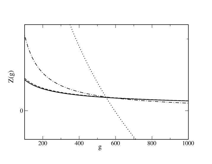
FIG. 1: Generating function $Z\left(g\right)$ as a function of the coupling parameter $g$. The solid line corresponds to the numerical evaluation of the exact solution (1) and the dashed line to the GBT solution (32). Dotted-dashed and dotted lines correspond to Borel resummation solutions (13) and (8) respectively. The value of $C$ minimizing the deviation of these approaches with respect to the exact solution (1) (solid line) was found to be equal to $-47.313$ and $3.572$ respectively. They were computed by the least square method in the range of values of $g$ given by the interval $[100,1000].$