Testing the Gaussian expansion method
in exactly solvable matrix models

Abstract:

The Gaussian expansion has been developed since early 80s as a powerful analytical method, which enables nonperturbative studies of various systems using ‘perturbative’ calculations. Recently the method has been used to suggest that 4d space-time is generated dynamically in a matrix model formulation of superstring theory. Here we clarify the nature of the method by applying it to exactly solvable one-matrix models with various kinds of potential including the ones unbounded from below and of the double-well type. We also formulate a prescription to include a linear term in the Gaussian action in a way consistent with the loop expansion, and test it in some concrete examples. We discuss a case where we obtain two distinct plateaus in the parameter space of the Gaussian action, corresponding to different large-$N$ solutions. This clarifies the situation encountered in the dynamical determination of the space-time dimensionality in the previous works.

1 Introduction

The Gaussian expansion is a powerful nonperturbative method, which has been applied to condensed matter physics and statistical physics extensively. Even at the lowest order, which is sometimes referred to as the self-consistent harmonic approximation, it allows us to understand fundamental properties of various systems at least qualitatively. In fact there exists a systematic way to improve the approximation, which we refer to as the Gaussian expansion method, but it is also called in the literature under various names such as improved mean field approximation, delta expansion and so on. The method has been worked out first in quantum mechanical systems [1, 2], where the expansion was shown to be convergent in some concrete examples [3], and it has been generalized to field theory later [4]. (The basic idea is also used in optimizing perturbation theory where the results depend on the renormalization scheme [2, 5, 6].) The most peculiar feature of this method, as emphasized by Stevenson [2], is that one obtains genuinely nonperturbative results — since never in the whole procedure does one attempt an expansion with respect to the coupling constant — and yet the required task is nothing more than familiar perturbative calculations based on Feynman diagrams.

Recently this method has been applied to superstring/M theories using their matrix model formulations. In Ref. [7] Kabat and Lifschytz proposed to use the Gaussian approximation in the Matrix Theory [8], which is conjectured to be a nonperturbative definition of M-theory in the infinite momentum frame. Indeed Refs. [9] were able to reveal interesting blackhole thermodynamics from the dual strong-coupling gauge theory. An earlier application of the Gaussian approximation to random matrix models can be found in Ref. [10].

In Ref. [11] two of the present authors (J.N. and F.S.) applied the Gaussian expansion method to the IIB matrix model [12], which is conjectured to be a nonperturbative definition of type IIB superstring theory in 10 dimensions. One of the most interesting questions in this model concerns the possibility that the 4d space-time [17] appears dynamically accompanied with the SSB of the SO(10) symmetry down to SO(4). From the path-integral point of view, this phenomenon may be caused by the phase of the fermion determinant [18], and Monte Carlo results support this mechanism [19] (Other possible mechanisms are discussed in Refs. [17, 20]). In Ref. [11] the same issue has been addressed analytically by using the Gaussian expansion method. The main idea was to consider various kinds of Gaussian action preserving only some subgroup of SO(10) and to identify the ‘true vacuum’ by comparing the corresponding free energy. Calculations up to the 3rd order showed that space-time preserving the SO(4) symmetry has the smallest free energy, and that the ratio of the extents in the four directions and the remaining six directions increases with the order. To our knowledge, this is the first time in history that the space-time dimensionality ‘4’ is suggested from the nonperturbative dynamics of superstring theory.

A lot of effort has then been made to increase the order of the expansion. In Ref. [22] it was noticed that Schwinger-Dyson equations can be used to reduce considerably the number of Feynman diagrams to be evaluated. In Ref. [23] a computer code has been written in order to automatize the task of listing up and evaluating all the Feynman diagrams. With these technical developments, the order of the expansion has now been increased up to the 7th order, and the results strengthened the conclusion of Ref. [11]. The nature of the method itself has also been clarified. In Ref. [22] the Gaussian expansion method was interpreted as an improved Taylor expansion, and the importance of identifying a plateau in the space of free parameters in the Gaussian action was recognized.

Although these new results in matrix models obtained by the Gaussian expansion method are quite encouraging and deserve further investigations, we consider it equally important to know the method itself by applying it to a well-understood system and to try to improve or refine the method. In our previous work [24] we applied the method to the bosonic version of the IIB matrix model, where Monte Carlo results [14] are available, and the convergence of the method has been demonstrated. We also developed a new technique to deal with the free parameters in the Gaussian action, which were conventionally determined by solving the ‘self-consistency equations’.

In this paper we attempt to gain more experience with the method by applying it to exactly solvable one-matrix models [25], which have been studied intensively in the context of two-dimensional quantum gravity and non-critical string theory. The Gaussian expansion has been carried out maximally up to the 18th order and the results are compared with the known exact results.

First we study the $\phi^{4}$ matrix model with various kinds of potential including the ones unbounded from below [25] and of the double-well type [26]. For the unbounded potential, it is known that a stable vacuum exists in the large-$N$ limit if the parameters of the potential satisfy a certain condition. In this case the Gaussian expansion converges and reproduces the exact results accurately. If the parameters are chosen such that there is no stable vacuum even in the large-$N$ limit, the Gaussian expansion does not converge either. Thus the method captures correctly the critical phenomenon associated with the overflow of the eigenvalues. For the double-well potential, on the other hand, we find that the results are in reasonable agreement with the exact values at low orders, but they start to oscillate violently as we go to higher orders.

Next we consider the $\phi^{3}$ matrix model. In this case the potential is always unbounded from below, but again a stable vacuum is known to exist in the large-$N$ limit if the parameters of the potential are chosen appropriately. A new ingredient here is that the model does not have the Z₂ symmetry unlike the $\phi^{4}$ matrix model, and therefore we have to include a linear term in the Gaussian action. We formulate a prescription to deal with the linear term in a way consistent with the loop expansion. Since we have two free parameters in the Gaussian action in this case, identifying a plateau in the parameter space becomes more nontrivial than in the $\phi^{4}$ matrix model. Here we find the histogram technique proposed in our previous paper [24] to be quite useful, and we do obtain results converging to the exact values.

Finally we reconsider the $\phi^{4}$ matrix model with the double-well potential, in which the Gaussian expansion method in its simplest form seems to fail as mentioned above. Here we redo the analysis with the inclusion of a linear term in the Gaussian action. Two types of linear term are considered, and for each case we obtain a plateau with different free energy. When we use a SU($N$) invariant but Z₂ breaking linear term, we obtain a plateau which corresponds to putting all the eigenvalues into a single well. When we use a linear term which has the ‘Z₂ symmetry’ but breaks the SU($N$) symmetry down to SU($N/2$)$\times$SU($N/2$), we obtain a plateau which corresponds to partitioning the eigenvalues equally into the two wells. The free energy for the latter is smaller in accord with exact results. This case therefore provides an example where we have more than one plateaus corresponding to different large-$N$ saddle-point solutions, but the true vacuum can still be determined by identifying the plateau which gives the smallest free energy. This supports the strategy taken to determine the dynamical space-time dimensionality in the aforementioned works in the IIB matrix model [11, 22, 23].

This paper is organized as follows. In Section 2 we study the $\phi^{4}$ matrix model with various types of potential. In Section 3 we study the $\phi^{3}$ matrix model, where we discuss how to treat a linear term in the Gaussian action systematically. In Section 4 we revisit the $\phi^{4}$ matrix model with the double-well potential including a linear term in the Gaussian action. Section 5 is devoted to summary and discussions. In Appendix A we discuss general large-$N$ saddle-point solutions in the $\phi^{4}$ matrix model with the double-well potential. In Appendices B and C we present the details of the calculations we have done in Section 4.

2 $\phi^{4}$ matrix model

In this Section we apply the Gaussian expansion method to the $\phi^{4}$ matrix model, which is exactly solvable and is known to exhibit nontrivial critical phenomena. We also give a brief review of the method in Section 2.2.1.

2.1 Exact solutions

The $\phi^{4}$ matrix model we study in this Section is defined by the partition function

$$Z = \int d^{N^{2}}\phi\,e^{-S},$$ (1)

$$S = N\frac{m}{2}{\rm tr\,}\phi^{2}+N\frac{g}{4}{\rm tr\,}\phi^{4},$$ (2)

where $\phi$ is a $N\times N$ hermitian matrix. The integration measure $d^{N^{2}}\phi$ is defined as $d^{N^{2}}\phi=\prod_{a=1}^{N^{2}}d\phi^{a}/{\sqrt{2\pi}}$, where $\phi^{a}$ are the coefficients in the expansion $\phi=\sum_{a}\phi^{a}T^{a}$ with respect to the U($N$) generators $T^{a}$ normalized as ${\rm tr\,}(T^{a}T^{b})=(1/2)\delta^{ab}$. By rescaling the variables $\phi$ as $\phi\mapsto\sqrt{|m|}^{-1}\phi$, one finds that the system can be characterized by the sign of $m$ and the effective coupling constant $g_{\rm eff}=g/m^{2}$.

In order to discuss the property of this model, it is convenient to look at the eigenvalues of the matrix $\phi$ . Let us therefore diagonalize $\phi$ as

$$\phi=V\Lambda V^{{\dagger}}\ ,$$ (3)

where $V$ is a unitary matrix and $\Lambda={\rm diag}(\lambda_{1},\cdots,\lambda_{N})$ is a real diagonal matrix. Integrating out the ‘angular variables’ $V$, one obtains the effective action for the eigenvalues $\lambda_{i}$ as

$$S_{\rm eff} = \sum_{i=1}^{N}V(\lambda_{i})-\sum_{i\neq j}\ln|\lambda_{i}-\lambda_{j}|\ ,$$ (4)

$$V(x) = N\left(\frac{m}{2}x^{2}+\frac{g}{4}x^{4}\right)\ ,$$ (5)

where the second term in (4) comes from the measure $d^{N^{2}}\phi$. Thus the effective theory for the eigenvalues may be regarded as a system of $N$ particles in the potential (5) with a logarithmic repulsive force between each pair. As a fundamental object, we introduce the eigenvalue distribution

$$\rho(x)=\left\langle\frac{1}{N}\sum_{i=1}^{N}\delta(x-\lambda_{i})\right\rangle\ .$$ (6)

Let us also define the free energy $F=-\ln Z$ and the observable $\left\langle\frac{1}{N}{\rm tr\,}\phi^{\ell}\right\rangle$, which can be written in terms of $\rho(x)$ as

$$\left\langle\frac{1}{N}{\rm tr\,}\phi^{\ell}\right\rangle=\int\,dx\,x^{\ell}\rho(x)\ .$$ (7)

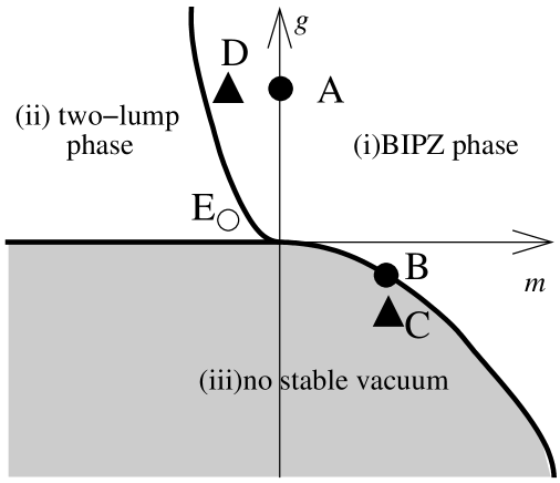
Figure 1: The phase diagram of the $\phi^{4}$ matrix model. The 5 points labeled as A, B, $\cdots$, E denote the set of parameters, for which we tested the Gaussian expansion method.

In the large-$N$ limit the phase diagram of the model consists of three regions : (i) the BIPZ phase, (ii) the two-lump phase, and (iii) no stable vacuum, as depicted in Fig. 1.

Let us first consider the case $m>0$ and $g>0$, in which the eigenvalue distribution $\rho(x)$ is given by [25]

$$\rho(x)=\frac{1}{\pi}\left(\frac{1}{2}gx^{2}+ga^{2}+\frac{1}{2}m\right)\sqrt{4a^{2}-x^{2}}$$ (8)

for $|x|\leq 2a$, where $a$ is defined by

$$a^{2}=\frac{2}{m+\sqrt{m^{2}+12g}}\ ,$$ (9)

and $\rho(x)=0$ otherwise. Note that $\rho(x)$ has a finite compact support $[-2a,2a]$ (We remind the reader that the large-$N$ limit is already taken here). The absence of penetration into the region $|x|>2a$ is due to the fact that the potential (5) grows linearly as $N$ goes to infinity, while the distribution does not collapse to the potential minimum due to the repulsive force between the $N$ particles. The free energy and the observables are given by

$$F(m,g) = N^{2}\left[\frac{1}{2}\ln N-\frac{1}{24}(ma^{2}-1)(ma^{2}-9)-\frac{1}{2}\ln(2a^{2})+O\left(\frac{\ln N}{N}\right)\right],$$ (10)

$$\left\langle\frac{1}{N}{\rm tr\,}\phi^{2}\right\rangle = \frac{1}{3}a^{2}(4-ma^{2})\mbox{~{}~{}~{}},\mbox{~{}~{}~{}}\left\langle\frac{1}{N}{\rm tr\,}\phi^{4}\right\rangle=\frac{a^{4}}{g}(3-ma^{2})\ .$$ (11)

Let us set $m$ to some positive value, and see what happens if one decreases $g$. Note that nothing singular happens at $g=0$, and the above expressions remain valid for $g<0$ as long as $m^{2}+12g$ inside the square root in eq. (9) is positive. Although the action becomes unbounded, the potential barrier grows with $N$ fast enough to prevent the eigenvalues from overflowing. For $g<-m^{2}/12$, however, the stable vacuum ceases to exist due to the overflow of the eigenvalues. At the critical point $g=-m^{2}/12$, the non-analyticity of $\rho(x)$ at the edge of the support ($x_{0}=\pm 2a$) changes from $|x-x_{0}|^{1/2}$ to $|x-x_{0}|^{3/2}$. This critical phenomenon plays a crucial role in the context of two-dimensional quantum gravity and non-critical string theory.

Let us next set $g$ to some positive value and see what happens if one decreases $m$. From (8) one finds that $\rho^{\prime\prime}(0)$ changes from negative to positive at $m=2\sqrt{g}$ , meaning that $\rho(x)$ starts to develop a double-peak structure. This occurs before $m$ reaches zero due to the repulsive force between the eigenvalues. From (8) one also finds that $\rho(0)$ decreases as one decreases $m$ and it finally becomes zero at $m=-2\sqrt{g}$. Beyond this point the eigenvalue distribution $\rho(x)$ will have two compact supports, and it is given explicitly by [26]

$$\rho(x)=\frac{1}{2\pi}g|x|\sqrt{(x^{2}-A_{-}^{2})(A_{+}^{2}-x^{2})}$$ (12)

for $A_{-}\leq|x|\leq A_{+}$, where $A_{\pm}$ is given by $A_{\pm}^{2}=(|m|\pm 2\sqrt{g})/g$ and $\rho(x)=0$ otherwise. At $m=-2\sqrt{g}$ the distribution (12) reduces to (8). The free energy and the observables are given by [26]

$$F(m,g) = N^{2}\left[\frac{1}{2}\ln N-\frac{3}{8}-\frac{1}{2}\ln 2-\frac{1}{4}\frac{m^{2}}{g}+\frac{1}{4}\ln g+O\left(\frac{\ln N}{N}\right)\right]\ ,$$ (13)

$$\left\langle\frac{1}{N}{\rm tr\,}\phi^{2}\right\rangle = \frac{|m|}{g}\mbox{~{}~{}~{}},\mbox{~{}~{}~{}}\left\langle\frac{1}{N}{\rm tr\,}\phi^{4}\right\rangle=\frac{m^{2}}{g^{2}}+\frac{1}{g}\ .$$ (14)

We call the phase that continues from the region $m>0$ and $g>0$ as the BIPZ phase, and the phase characterized by the two compact supports of the eigenvalue distribution as the two-lump phase.

2.2 The Gaussian expansion method

As we have seen in the previous Section, the simple one-matrix model exhibits nontrivial critical phenomena associated with the eigenvalue distribution. These phenomena are certainly nonperturbative in the sense that it cannot be seen by perturbative expansion with respect to $g_{\rm eff}=g/m^{2}$. The aim of this Section is to apply the Gaussian expansion method to this model and to see if it reproduces these critical phenomena correctly.

2.2.1 A brief review

We will first illustrate the idea of the Gaussian expansion method using the $\phi^{4}$ matrix model as an example. Let us denote the quadratic term and the quartic term in the action (2) as $S_{2}$ and $S_{4}$ so that $S=S_{2}+S_{4}$. Ordinary loop expansion can be formulated as follows : (i) consider the action

$$S_{\rm PT}(\lambda)=\frac{1}{\lambda}(S_{2}+S_{4})\ ,$$ (15)

(ii) calculate free energy and observables as an expansion with respect to $\lambda$ up to some finite order, and (iii) set $\lambda=1$. Equivalence to the perturbative expansion with respect to $g_{\rm eff}=g/m^{2}$ can be easily seen by rescaling the variables as $\phi\mapsto\sqrt{\lambda/|m|}\,\phi$. The Gaussian expansion method simply amounts to replacing the action (15) by

$$S_{\rm GEM}(t;\lambda)=\,\frac{1}{\lambda}\,\Bigl{[}\Bigl{\{}S_{0}+\lambda(S_{2}-S_{0})\Bigr{\}}+S_{4}\Bigr{]}\ ,$$ (16)

where $S_{0}$ is taken to be the SU($N$) invariant Gaussian action

$$S_{0}=\frac{Nt}{2}{\rm tr\,}\phi^{2}$$ (17)

with a real positive parameter $t$, which is left arbitrary at this point. Note that both (15) and (16) reduces to the original action (2) if one sets $\lambda=1$. The Gaussian expansion method can also be viewed as a loop expansion but with the ‘classical action’ $(S_{0}+S_{4})$ and the ‘one-loop counterterms’ $(S_{2}-S_{0})$. Note, however, that the method cannot be viewed as an expansion with respect to any parameter in the original action unlike (15), except when one sets $t=m$, for which one simply retrieves the ordinary perturbation theory. In fact the freedom in changing the parameter $t$ in the Gaussian action (17) plays a crucial role in this method.

To make things more transparent, let us rescale $\phi$ as $\phi\mapsto\sqrt{\lambda}\,\phi$ so that the partition function takes the form

$$Z = \int d^{N^{2}}\phi\,e^{-(S_{\rm cl}+S_{\rm c.t.})}\ ,$$ (18)

$$S_{\rm cl}(t;\lambda) = S_{0}+\lambda S_{4}~{}~{}~{},~{}~{}~{}S_{\rm c.t.}(t;\lambda)=\lambda(S_{2}-S_{0})\ .$$ (19)

Thus in the present example the Gaussian expansion can be viewed also as an expansion with respect to $(S-S_{0})$, the difference of the original action from the Gaussian action. However this is peculiar to the models with actions containing only quadratic and quartic terms, and it is not the case in general (See Section 3). In earlier formulation [7, 11] the expansion was first made with respect to $(S-S_{0})$, and then it was reorganized in such a way that it becomes consistent with the loop expansion. Here we have chosen to take a shorter path.

In actual calculations, the ‘one-loop counter terms’ can be incorporated easily by noticing the relation

$$S_{\rm cl}(t;\lambda)+S_{\rm c.t.}(t;\lambda)=S_{\rm cl}(t+\lambda(m-t);\lambda)\ .$$ (20)

Namely the calculation of a physical quantity in the Gaussian expansion proceeds in two steps; (i) obtain the $\lambda$-expansion of the quantity using the ‘classical action’ $S_{\rm cl}(t;\lambda)$, (ii) shift the parameter $t$ by $\lambda(m-t)$ and reorganize the expansion with respect to $\lambda$. In general the first step can be done by ordinary Feynman diagrammatic calculations, where the use of Schwinger-Dyson equations reduces the number of diagrams considerably [22]. The large-$N$ limit can be taken, if one wishes, by simply retaining the planar diagrams only. (This results in considerable simplification in the matrix model applications, but it is definitely not the main point of the Gaussian expansion method itself.) In fact in the present case where we know the exact results for the ‘classical action’ $S_{\rm cl}(t;\lambda)$ [25], the first step can be done with little effort using softwares for symbolic manipulations like Mathematica. This allows us to test the Gaussian expansion method at very high orders (we went maximally up to the 18th order).

Let us move on to the results obtained by the Gaussian expansion method. We compute the ‘free energy density’ defined by

$$f=\lim_{N\to\infty}\left\{\frac{F}{N^{2}}-\frac{1}{2}\ln N\right\}\ ,$$ (21)

where the second term is subtracted in order to make the quantity finite in the large-$N$ limit. For illustrative purposes, we consider the case $g=1$, $m=0$ (the point A in Fig. 1), which was also studied in Refs. [22, 23]. Let us recall that the expansion parameter in ordinary perturbation theory is $g_{\rm eff}=g/m^{2}$ and the convergence radius is known to be $1/12$. Therefore the above choice of parameters corresponds to the strong coupling limit, which is of course beyond the reach of ordinary perturbation theory.

Figure 2: (Left) The free energy density $f$ calculated by the Gaussian expansion method is plotted as a function of $1/t$ for $g=1$, $m=0$. Each curve corresponds to the order 3, 6, 9, 12, 15, 18. The horizontal line represents the exact value $f=-3/8-\log(2/\sqrt{3})/2=-0.44692\cdots$. (Right) The free energy density $f$ extracted at the order 2 , $\cdots$, 18 by the histogram technique from the results of the Gaussian expansion for various $1/t$. (When we make a histogram, we used the region $0.01\leq 1/t\leq 1$.) The ‘error bars’ represent the theoretical uncertainty estimated by the same technique. The order 1 result ($f=-0.423287$) lies outside the displayed region. The horizontal line represents the exact result.

In Fig. 2 (left) we plot the free energy obtained at the order 3, 6, 9, 12, 15, 18 as a function of $1/t$. As one can see also from the figure, the result of the Gaussian expansion generically depends on the free parameter $t$ in the Gaussian action (17). However, since $t$ is a parameter which is introduced by hand, the result should not depend much on it in the region of $t$ where the expansion becomes valid, if such a region exists at all. Indeed at sufficiently high orders we observe the formation of a plateau, meaning that there exists a certain range of $t$ where the result becomes almost independent of $t$. Moreover the height of the plateau agrees very accurately with the exact result represented by the horizontal line. In old literature the free parameter ($t$ in the present case) was determined in such a way that the result becomes most insensitive to the change of the parameter. This strategy was named as ‘the principle of minimum sensitivity’ [2]. The importance of the formation of a plateau has been first recognized in Ref. [22].

Given this new insight, we still have to develop some technique to identify a plateau and to extract its height in order to make a concrete prediction. Note also that the plateau is not completely flat but has some small fluctuations in practice. This causes some theoretical uncertainty in the prediction from the method, and it is desirable to be able to estimate its order of magnitude. In Ref. [24] we have developed a technique based on histograms. Fig. 2 (right) shows the results obtained for the present case. The ‘error bars’ represent an estimate for the theoretical uncertainty explained above. Clearly the result converges to the exact value within the first several orders.

2.2.2 Unbounded potential ($g<0$, $m>0$)

Let us move on to the $g<0$, $m>0$ case, for which the potential becomes unbounded from below. As we discussed in Section 2.1, a stable vacuum continues to exist for $g\geq-m^{2}/12$ in the large-$N$ limit. In Fig. 3 (left) we show the free energy as a function of $1/t$ at the critical point $g=-1/12$, $m=1$ (the point B in Fig. 1). We observe the formation of a clear plateau. The results for $g>-m^{2}/12$ were equally successful. It is noteworthy that the Gaussian expansion method can reproduce the large-$N$ solution even in the case of the unbounded potential.

Figure 3: (Left) The free energy density $f$ is plotted as a function of $1/t$ for $g=-\frac{1}{12}$, $m=1$ (critical point). Each curve corresponds to the order 3, 6, 9, 12, 15, 18. The horizontal line represents the exact value $f=7/24-\log 2=-0.40148\cdots$. (Right) The free energy density $f$ is plotted as a function of $1/t$ for $g=-\frac{1}{10}$, $m=1$. Each curve corresponds to the order 3, 6, 9, 12, 15, 18.

In Fig. 3 (right) we show the results for $g=-\frac{1}{10}$, $m=1$ (the point C in Fig. 1), which is slightly below the critical point. At each order we see a plateau-like region, but the slope in that region increases with the order (Note the striking difference from the figure on the left). Thus the Gaussian expansion method seems to know the absence of a stable vacuum with this choice of parameters. This example also confirms the importance of the plateau formation in the method.

It is interesting to see how the plateau formation ceases to occur when we cross the critical point. This is reflected in the peculiar situation at the critical point. The plateaus in Fig. 3 (left) do not have the tiny oscillations which become visible upon magnification in Fig. 2 (left). In fact in Fig. 3 (left) there is only one stationary point at each order we studied, and the free energy at that point coincides with the exact value at the orders $\geq 2$. The stationary point disappears as soon as we cross the critical point.

2.2.3 Double-well potential ($g>0$, $m<0$)

Let us then consider the case with the double-well potential. The system undergoes a phase transition from the BIPZ phase to the two-lump phase at $m=-2\sqrt{g}$. Fig. 4 (left) shows the free energy as a function of $1/t$ for $g=1$, $m=-1$ (the point D in Fig. 1). Although the chosen parameters are still well within the BIPZ phase, we observe an oscillating behavior which becomes more and more violent as the order is increased beyond the order 9. This is also reflected in Fig. 4 (right), which shows the results extracted by the histogram technique at each order. The oscillation becomes even worse as we go to further negative $m$.

Figure 4: (Left) The free energy density $f$ is plotted as a function of $1/t$ for $g=1$, $m=-1$. Each curve corresponds to the order 3, 6, 9, 12, 15, 18. The horizontal line represents the exact value. (Right) The free energy density $f$ obtained by the histogram prescription at the order 2, …, 18 for $g=1$, $m=-1$. (When we make a histogram, we used the region $0.01\leq 1/t\leq 1$.) The order 1 result ($f=-0.846574$) lies outside the displayed region. The horizontal line represents the exact result $f=-0.933705\cdots$.

Thus we find that the Gaussian expansion method in its simplest form does not work in the case of the double-well potential. (A similar result was obtained in the quantum mechanics of a particle in a double-well potential [1].) This is understandable if we recall that the method amounts to expanding the theory around $\phi=0$, which is a local maximum of the double-well potential. We will reconsider the present example in Section 4 including a linear term in the Gaussian action.

3 $\phi^{3}$ matrix model

In this Section we will test the Gaussian expansion method in the $\phi^{3}$ matrix model, which is also exactly solvable. In this model the potential is always unbounded from below, but a stable vacuum exists in the large-$N$ limit when the parameters in the potential are chosen appropriately. The situation is thus similar to the $\phi^{4}$ model with the unbounded potential, but the main issue here is that we have to include a linear term in the Gaussian action due to the absence of the Z₂ symmetry. We will treat it in a way consistent with the loop expansion, and check the result against the exact solution. As a result of having a linear term, we have two free parameters, which makes the identification of a plateau somewhat more nontrivial than in the previous Section. The histogram technique turns out to be quite useful.

3.1 Exact solutions

The $\phi^{3}$ matrix model is defined by the partition function

$$Z = \int d^{N^{2}}\phi\,e^{-S},$$ (1)

$$S = N\frac{1}{2}\,{\rm tr\,}\phi^{2}+N\frac{g}{3}\,{\rm tr\,}\phi^{3}\ ,$$ (2)

where $\phi$ is a $N\times N$ hermitian matrix, and the measure $d^{N^{2}}\phi$ is the same as in the $\phi^{4}$ matrix model. Although the action (2) is unbounded from below, the theory is well-defined in the large-$N$ limit for $g^{2}\leq g_{c}^{2}\equiv\frac{1}{12\sqrt{3}}$.

The exact results for the free energy and observables are given by [25]

$$F(g) = N^{2}\left[\frac{1}{2}\ln N+\frac{1}{2}\ln\frac{1+2\sigma}{2}-\frac{1}{3}\frac{\sigma(3\sigma^{2}+6\sigma+2)}{(1+\sigma)(1+2\sigma)^{2}}+O\left(\frac{\ln N}{N}\right)\right]\ ,$$ (3)

$$\left\langle\frac{1}{N}{\rm tr\,}\phi\right\rangle = -g\frac{1+3\sigma}{(1+\sigma)(1+2\sigma)^{2}}~{}~{}~{},~{}~{}~{}\left\langle\frac{1}{N}{\rm tr\,}\phi^{2}\right\rangle=\frac{1+3\sigma}{(1+\sigma)(1+2\sigma)^{2}}\ ,$$ (4)

where $\sigma$ is the largest solution of the equation $\sigma(1+\sigma)(1+2\sigma)=-2g^{2}$. The above expressions are valid for $|g|\leq g_{c}$. For $|g|>g_{c}$, on the other hand, the system does not have a stable vacuum even in the large-$N$ limit. In what follows we assume $g\geq 0$ without loss of generality due to the duality under the sign flip of $g$.

3.2 Systematic treatment of a linear term in the Gaussian action

Let us denote the quadratic and cubic terms in the action (2) as $S_{2}$ and $S_{3}$ so that the action reads $S=S_{2}+S_{3}$. Similarly to (16), the Gaussian expansion amounts to considering the action

$$S_{\rm GEM}(t,h;\lambda)=\,\frac{1}{\lambda}\,\Bigl{[}\Bigl{\{}S_{0}+\lambda(S_{2}-S_{0})\Bigr{\}}+S_{3}\Bigr{]}\ .$$ (5)

Since the action (2) does not have the Z₂ symmetry unlike the $\phi^{4}$ matrix model, the $S_{0}$ in (5) should include a linear term as

$$S_{0}=S_{\rm G}+S_{\rm L},$$

$$S_{\rm G}=\frac{N}{2}t\,{\rm tr\,}\phi^{2},\quad S_{\rm L}=Nh\,{\rm tr\,}\phi\ ,$$ (6)

where the real parameters $t$ and $h$ are arbitrary at this point. Free energy and observables are calculated as an expansion with respect to $\lambda$, and $\lambda$ is set to one eventually. This procedure yields a loop expansion with the ‘classical action’ $(S_{0}+S_{3})$ and the ‘one-loop counter term’ $(S_{2}-S_{0})$.

As in the $\phi^{4}$ matrix model, let us rescale $\phi$ as $\phi\mapsto\sqrt{\lambda}\phi$ so that the partition function takes the form

$$Z = \int d^{N^{2}}\phi\,e^{-(S_{\rm cl}+S_{\rm c.t.})}\ ,$$ (7)

$$S_{\rm cl}(t,h;\lambda) = S_{\rm G}+\frac{1}{\sqrt{\lambda}}S_{\rm L}+\sqrt{\lambda}S_{3}~{}~{}~{},~{}~{}~{}S_{\rm c.t.}(t,h;\lambda)=\lambda(S_{2}-S_{\rm G})-\sqrt{\lambda}S_{\rm L}\ .$$ (8)

Thus the Gaussian expansion in the present case cannot be viewed as an expansion with respect to $(S-S_{0})$ unlike the $\phi^{4}$ matrix model. The ‘counter terms’ $S_{\rm c.t.}$ in (8) can be easily implemented by using the relation

$$S_{\rm cl}(t,h;\lambda)+S_{\rm c.t.}(t,h;\lambda)=S_{\rm cl}(t+\lambda(1-t),h-\lambda h;\lambda)\ .$$ (9)

Namely the calculation of a physical quantity in the Gaussian expansion proceeds in two steps; (i) obtain the $\lambda$-expansion of the quantity using the ‘classical action’ $S_{\rm cl}(t,h;\lambda)$, (ii) shift the parameters $t$ and $h$ by $\lambda(1-t)$ and $(-\lambda h)$ respectively and reorganize the expansion with respect to $\lambda$.

As usual we eliminate the linear term in $S_{\rm cl}(t,h;\lambda)$ by shifting the variables as $\phi=\tilde{\phi}+\frac{\alpha}{\sqrt{\lambda}}{\bf 1}$, where the parameter $\alpha$ should satisfy

$$g\alpha^{2}+t\alpha+h=0\ .$$ (10)

The ‘classical action’ then becomes

$$S_{\rm cl}(t,h;\lambda)=C+N\frac{1}{2}\tilde{t}\,{\rm tr\,}\tilde{\phi}^{2}+\sqrt{\lambda}N\frac{1}{3}g\,{\rm tr\,}\tilde{\phi}^{3}\ ,$$ (11)

where $C$ and $\tilde{t}$ are given by

$$C = N^{2}\frac{1}{\lambda}\left(\frac{1}{2}\alpha^{2}t+h\alpha+\frac{1}{3}g\alpha^{3}\right)\ ,$$ (12)

$$\tilde{t} = t+2g\alpha\ .$$ (13)

Thus the problem reduces to the conventional perturbative expansion in the $\phi^{3}$ matrix model. Note that the constant term $C$ in (11) contributes to the ‘order-$(-1)$ term’ in the $\lambda$-expansion of free energy.

Figure 5: (Left) Free energy density at the order 5 is plotted as a function of $1/\tilde{t}$ and $h$. (Right) The histogram of the free energy density. (When we make a histogram, we used the region $0.02\leq 1/\tilde{t}\leq 2$, $-3\leq h\leq 5$. The bin size is taken to be $10^{-5}$.) The vertical line represents the exact result $f=-0.389176\cdots$.

Figure 6: The same as Fig. 5 but for the order 15.

Eq. (10) has two solutions $\alpha=\frac{1}{2g}(-t\pm\sqrt{t^{2}-4gh})$, which correspond to $\tilde{t}=\pm\sqrt{t^{2}-4gh}$ respectively. Since $\tilde{t}$ is the coefficient of the quadratic term in eq. (11), it should be positive in order for the Gaussian expansion to be well-defined. This forces us to take

$$\alpha=\frac{1}{2g}(-t+\sqrt{t^{2}-4gh}).$$ (14)

Considering that $1/\tilde{t}$ has the meaning as the tree-level propagator, we shall plot the result of the Gaussian expansion obtained for various $t$ and $h$ as a function of $1/\tilde{t}$ and $h$. For each $\tilde{t}$ and $h$ satisfying $\tilde{t}^{2}+4gh>0$, we obtain results corresponding to $t>0$ and $t<0$. It turned out, however, that the plateau mainly develops in the branch corresponding to $t>0$. We therefore plot the results for $t>0$ in what follows.

Here we show our results at the critical point $g^{2}=g_{c}^{2}\equiv\frac{1}{12\sqrt{3}}$. In Fig. 5 (left) we plot the free energy density defined by (21) as a function of $1/\tilde{t}$ and $h$ at the order 5. We observe a clear plateau. On the right we show the corresponding histogram, which has a sharp peak at the exact value. Fig. 6 shows the results at the order 15. The plateau extends and as a result the peak of the histogram becomes higher. (In the present case we were not able to obtain a reasonable estimate for the uncertainty because the plateau turned out to be too flat. This seems to be a peculiar feature at the critical point.) We have checked that observables such as $\langle\frac{1}{N}{\rm tr\,}\phi\rangle$ and $\langle\frac{1}{N}{\rm tr\,}\phi^{2}\rangle$ also agree with the exact results very accurately. These results support the correctness of the way we treated the linear term in the Gaussian action.

4 $\phi^{4}$ matrix model with the double-well potential, revisited

In this Section we will revisit the $\phi^{4}$ matrix model with the double-well potential, where the simplest version of the Gaussian expansion seems to fail (See Section 2.2.3). Here we would like to perform the expansion including a linear term as we formulated in the previous Section. In fact we are going to consider two kinds of linear term. One is the same as in the $\phi^{3}$ matrix model, and the other is a linear term with a ‘twist’ which breaks the SU($N$) symmetry down to SU($N/2$)$\times$SU($N/2$). For each case we obtain a plateau corresponding to different large-$N$ solutions. The first one corresponds to putting all the eigenvalues into one well, and the second one corresponds to partitioning the eigenvalues equally into the two wells. In accord with the exact results, the free energy is smaller for the latter, which corresponds to the ‘true vacuum’. The present example supports the validity of the strategy adopted in the dynamical determination of the space-time dimensionality in the IIB matrix model [11, 22, 23].

4.1 Single-lump solution in the double-well potential

In fact the $\phi^{4}$ matrix model with the double-well potential has a one-parameter family of large-$N$ solutions corresponding to different partitioning of the $N$ eigenvalues into the two wells (See Appendix A). The solution (12) corresponds to the equal partitioning, and it has the smallest free energy. For asymmetric partitioning, the free energy becomes larger due to the repulsive force and due also to the increase of the potential energy. These asymmetric large-$N$ solutions are stable, however, against tunneling of the eigenvalues because the potential barrier grows linearly with $N$. The situation is analogous to the existence of a stable large-$N$ solution in spite of the unbounded potential discussed in Section 2.1.

Here we will consider the extreme case where all the eigenvalues are put into one well. The exact results can be readily obtained by applying the technique used in Ref. [25]. The eigenvalue distribution has the form

$$\rho(x)=\frac{1}{2\pi}\left\{gx^{2}+\sqrt{g\sigma}x-\frac{2}{3}(|m|-\sigma)\right\}\sqrt{(x-B_{-})(B_{+}-x)}$$ (15)

for $B_{-}\leq x\leq B_{+}$ and $\rho(x)=0$ otherwise. The edges of the support are given by

$$B_{\pm}=\sqrt{\frac{\sigma}{g}}\pm\sqrt{\frac{2}{3g}(|m|-\sigma)}\ ,$$ (16)

and the parameter $\sigma$ is defined as

$$\sigma=\frac{3|m|+2\sqrt{m^{2}-15g}}{5}\ .$$ (17)

The free energy and observables are obtained as

$$F = N^{2}\left[\frac{1}{2}\ln N-\frac{3}{8}+\frac{1}{2}\ln\frac{5\sigma-|m|}{4}-\frac{43}{180}\frac{m^{2}}{g}\right.$$ (18)

$$\left.\mbox{~{}~{}~{}~{}~{}~{}~{}}+\left(\frac{5}{3}-\frac{2}{45}\frac{m^{2}}{g}\right)\frac{|m|}{5\sigma-|m|}+O\left(\frac{\ln N}{N}\right)\right]\ ,$$

$$\left\langle\frac{1}{N}{\rm tr\,}\phi\right\rangle = 4\sqrt{\frac{\sigma}{g}}\frac{\sigma}{5\sigma-|m|}~{},~{}\left\langle\frac{1}{N}{\rm tr\,}\phi^{2}\right\rangle=\frac{41}{45}\frac{|m|}{g}+\frac{16}{3}\left(\frac{1}{15}\frac{m^{2}}{g}-1\right)\frac{1}{5\sigma-|m|}\ .$$ (19)

As can be seen from (17), the single-lump solution exists for $0<g/m^{2}\leq 1/15$, while the Z₂-symmetric solution (12) corresponding to the ‘true vacuum’ exists for $0<g/m^{2}\leq 1/4$. It is understandable that the critical $g/m^{2}$ is larger for the latter (the potential wells become shallower as $g/m^{2}$ increases).

4.2 Gaussian expansion method with a linear term

We will see that the single-lump solution (15) can be reproduced by the Gaussian expansion method if we include a linear term. The formulation is quite analogous to the $\phi^{3}$ matrix model, so the description will be brief. Instead of (5) we consider the action

$$S_{\rm GEM}(t,h;\lambda)=\,\frac{1}{\lambda}\,\Bigl{[}\Bigl{\{}S_{0}+\lambda(S_{2}-S_{0})\Bigr{\}}+S_{4}\Bigr{]}\ ,$$ (20)

where $S_{0}$ includes the linear term $S_{\rm L}$ as in (6), while $S_{2}$ and $S_{4}$ are the same as in Section 2.2.1. Rescaling the variables as $\phi\mapsto\sqrt{\lambda}\,\phi$, we obtain

$$Z = \int d^{N^{2}}\phi\,e^{-(S_{\rm cl}+S_{\rm c.t.})}\ ,$$ (21)

$$S_{\rm cl}(t,h;\lambda) = S_{\rm G}+\frac{1}{\sqrt{\lambda}}S_{\rm L}+\lambda S_{4}~{}~{}~{},~{}~{}~{}S_{\rm c.t.}(t,h;\lambda)=\lambda(S_{2}-S_{\rm G})-\sqrt{\lambda}S_{\rm L}\ .$$ (22)

The ‘one-loop counter terms’ can be incorporated by using the relation

$$S_{\rm cl}(t,h;\lambda)+S_{\rm c.t.}(t,h;\lambda)=S_{\rm cl}(t+\lambda(m-t),h-\lambda h;\lambda)\ .$$ (23)

After eliminating the linear term in $S_{\rm cl}(t,h;\lambda)$ by shifting the variable as $\phi=\tilde{\phi}+\frac{\alpha}{\sqrt{\lambda}}{\bf 1}$, the ‘classical action’ becomes

$$S_{\rm cl}(t,h;\lambda)=C+N\frac{1}{2}\tilde{t}\,{\rm tr\,}\tilde{\phi}^{2}+\sqrt{\lambda}N\frac{1}{3}\tilde{g}\,{\rm tr\,}\tilde{\phi}^{3}+\lambda N\frac{1}{4}g\,{\rm tr\,}\tilde{\phi}^{4}\ ,$$ (24)

where $C$, $\tilde{t}$ and $\tilde{g}$ are given by

$$C = N^{2}\frac{1}{\lambda}\frac{\alpha}{4}(3h+t\alpha),$$ (25)

$$\tilde{t} = t+3g\alpha^{2},$$ (26)

$$\tilde{g} = 3g\alpha\ .$$ (27)

Thus the problem reduces to the conventional perturbative expansion in the one-matrix model with both $\phi^{3}$ and $\phi^{4}$ interactions. As in the previous cases, we can utilize the large-$N$ solution, which can be obtained by the same method [25]. See Appendix B for the details.

The shift parameter $\alpha$ should satisfy

$$g\alpha^{3}+t\alpha+h=0\ ,$$ (28)

which has three solutions. For $t>0$ they are given by

$$\alpha_{1} = \frac{1}{18^{1/3}\sqrt{g}}\,\Bigl{(}-G_{+}^{1/3}+G_{-}^{1/3}\Bigr{)}\ ,$$

$$\alpha_{2} = \frac{1}{18^{1/3}\sqrt{g}}\,\Bigl{(}e^{i\pi/3}G_{+}^{1/3}-e^{-i\pi/3}G_{-}^{1/3}\Bigr{)}\ ,$$

$$\alpha_{3} = \frac{1}{18^{1/3}\sqrt{g}}\,\Bigl{(}e^{-i\pi/3}G_{+}^{1/3}-e^{i\pi/3}G_{-}^{1/3}\Bigr{)}\ ,$$ (29)

while for $t<0$ they are given by

$$\alpha_{1} = \frac{1}{18^{1/3}\sqrt{g}}\,\Bigl{(}e^{-i\pi/3}G_{+}^{1/3}+G_{-}^{1/3}\Bigr{)}\ ,$$

$$\alpha_{2} = \frac{1}{18^{1/3}\sqrt{g}}\,\Bigl{(}-G_{+}^{1/3}-e^{-i\pi/3}G_{-}^{1/3}\Bigr{)}\ ,$$

$$\alpha_{3} = \frac{1}{18^{1/3}\sqrt{g}}\,e^{i\pi/3}\Bigl{(}G_{+}^{1/3}-G_{-}^{1/3}\Bigr{)}\ ,$$ (30)

where we have introduced $G_{\pm}\equiv\pm 9\sqrt{g}h+\sqrt{81gh^{2}+12t^{3}}$. Among the three branches, two of them ($\alpha_{2}$ and $\alpha_{3}$ for $t>0$, $\alpha_{1}$ and $\alpha_{2}$ for $t<0$) are mapped to each other under the sign flip of $h$, while the remaining one is symmetric. This structure is a consequence of the Z₂ symmetry of the $\phi^{4}$ model. Requiring $\tilde{t}$ to be real positive we are left with the following four cases.

$$\begin{array}[]{ll}\alpha=\alpha_{1}&\quad\mbox{for }\quad t>0\ ,\\ \alpha=\alpha_{1}&\quad\mbox{for }\quad t<0,\quad h\leq-\sqrt{\frac{4}{27g}}|t|^{3/2}\ ,\\ \alpha=\alpha_{2}&\quad\mbox{for }\quad t<0,\quad h\geq\sqrt{\frac{4}{27g}}|t|^{3/2}\ ,\\ \alpha=\alpha_{1},\alpha_{2}&\quad\mbox{for }\quad t<0,\quad-\sqrt{\frac{4}{27g}}|t|^{3/2}<h<\sqrt{\frac{4}{27g}}|t|^{3/2}\ .\end{array}$$ (31)

As in the $\phi^{3}$ model, we plot the result of the Gaussian expansion as a function of $1/\tilde{t}$ and $h$. In what follows we show only the branch which includes the plateau in the $h>0$ regime.

We present the result for the free energy at $g=1/15$ and $m=-1$ (the point E in Fig. 1), which is the critical point for the existence of the single-lump solution. In Fig. 7 (left) the free energy density $f$ at the order 3 is plotted as a function of $1/\tilde{t}$ and $h$. The figure on the right shows the corresponding histogram. (Here again we were not able to obtain a reasonable estimate for the uncertainty because the plateau turned out to be too flat.) The formation of a plateau is clearly observed and the histogram has a sharp peak at the exact result. Fig. 8 shows the results at the order 6. The plateau extends to larger area, and consequently the peak of the histogram becomes higher.

Figure 7: (Left) Free energy density at the order 3 is plotted as a function of $1/\tilde{t}$ and $h$ for $g=1/15$ and $m=-1$. (Right) The histogram of the free energy density. (When we make a histogram, we used the region $0.02\leq 1/\tilde{t}\leq 2$, $-5\leq h\leq 5$. The bin size is taken to be $10^{-5}$.) The vertical line represents the exact result $f=-3.80491\cdots$.

Figure 8: The same as Fig. 7 but for the order 6.

4.3 Gaussian expansion method with a twisted linear term

In this Section we attempt to reproduce the ‘true vacuum’, which corresponds to partitioning the eigenvalues equally into the two wells. The failure of the Gaussian expansion method in Section 2.2.3 may be attributed to the fact that the $\lambda$-expansion with the action (16) corresponds to expanding around the classical solution $\phi=0$, where the double-well potential becomes locally maximum. (When we say ‘classical’, we regard the parameter $\lambda$ as the Planck constant $\hbar$.) Here we will take the Gaussian term $S_{0}$ in the action (16) in such a way that the classical solution becomes proportional to

$$J=\sigma_{3}\otimes{1\!\!1}_{N/2}={\rm diag}(\underbrace{1,\cdots,1}_{N/2},\underbrace{-1,\cdots,-1}_{N/2})\ ,$$ (32)

where and henceforth $\sigma_{a}$ denote Pauli matrices. This can be achieved by considering the action (20) with a ‘twisted linear term’ given by

$$S_{\rm L}=Nh\,{\rm tr\,}(J\phi)\ .$$ (33)

This term breaks the SU($N$) symmetry down to SU($N/2$)$\times$SU($N/2$), but the total action (20) has the ‘Z₂ symmetry’

$$\phi\mapsto-T\phi T^{\dagger}~{}~{}~{},~{}~{}~{}T=\sigma_{1}\otimes{1\!\!1}_{N/2}\ .$$ (34)

We expect that other large-$N$ solutions described in Appendix A can be reproduced by considering the asymmetric twist

$$J^{\prime}={\rm diag}(\underbrace{1,\cdots,1}_{n_{\rm L}},\underbrace{-1,\cdots,-1}_{n_{\rm R}})~{}~{}~{},~{}~{}~{}n_{\rm L}+n_{\rm R}=N$$ (35)

instead of (32).

After eliminating the linear term by shifting the variable as $\phi=\tilde{\phi}+\frac{\alpha}{\sqrt{\lambda}}J$, the ‘classical action’ becomes

$$S_{\rm cl}(t,h;\lambda)=C+N\frac{1}{2}\tilde{t}\,{\rm tr\,}\tilde{\phi}^{2}+N\frac{1}{2}g\,\alpha^{2}\,{\rm tr\,}(J\phi J\phi)+\sqrt{\lambda}N\tilde{g}\,{\rm tr\,}(J\phi^{3})+\lambda N\frac{1}{4}g\,{\rm tr\,}\tilde{\phi}^{4}\ ,$$ (36)

where $C$, $\tilde{t}$ and $\tilde{g}$ are given by

$$C = N^{2}\frac{1}{\lambda}\frac{\alpha}{4}(3h+t\alpha),$$ (37)

$$\tilde{t} = t+2g\,\alpha^{2},$$ (38)

$$\tilde{g} = g\,\alpha\ .$$ (39)

By decomposing the matrix $\phi$ as

$$\phi=\sum_{a=1}^{4}\sigma_{a}\otimes\varphi_{a}\ ,$$ (40)

where $\sigma_{4}$ is a $2\times 2$ unit matrix and $\varphi_{a}$ are $N/2\times N/2$ hermitian matrices, the quadratic term in (36) becomes

$$S_{\rm quad} = N(\tilde{t}-g\,\alpha^{2})\,{\rm tr\,}\{(\varphi_{1})^{2}+(\varphi_{2})^{2}\}$$ (41)

$$+N(\tilde{t}+g\,\alpha^{2})\,{\rm tr\,}\{(\varphi_{3})^{2}+(\varphi_{4})^{2}\}\ .$$

In order to make the Gaussian expansion well-defined, we therefore have to require $\tilde{t}-g\,\alpha^{2}>0$, which means

$$t+g\,\alpha^{2}>0\ .$$ (42)

Figure 9: (Left) A contour plot of the free energy density as a function $1/(\tilde{t}-g\alpha^{2})$ and $h$ at the order 1 for $m=-1$, $g=\frac{1}{15}$. 40 contours for $f=-5.5+0.02\times n$ $(n=1,\cdots,40)$ are plotted. The blank region near the right-up corner means that the calculated free energy density does not fall in the specified region of $f$. (Right) The same as in the figure on the left but for the order 3. The plateau has grown diagonally from the left-top to the right-bottom. The meaning of the blank regions is the same as in the left figure.

The equation for $\alpha$ is the same as (28), so the solutions are (29), (30). Combining (42) and (28), one finds that $\alpha$ and $h$ should have opposite signs. Thus the allowed real solution for $\alpha$ is determined uniquely in the present case as

$$\begin{array}[]{ll}\alpha=\alpha_{1}&\quad\mbox{for }\quad t>0\\ \alpha=\alpha_{1}&\quad\mbox{for }\quad t<0,\,h<0\\ \alpha=\alpha_{2}&\quad\mbox{for }\quad t<0,\,h>0\ .\end{array}$$ (43)

Note that $t$ and $h$ can take any real values except for $t<0$ and $h=0$. As before we plot the results obtained for various $t$ and $h$ as a function of $1/(\tilde{t}-g\alpha^{2})$ and $h$. In the present case we have only one branch. Since the figure is invariant under the reflection $h\mapsto-h$ due to the Z₂ symmetry, we will restrict ourselves to $h>0$ in what follows.

Since the one-matrix model with the SU($N$) breaking terms (36) cannot be solved exactly with the known techniques, we have to perform diagrammatic calculations explicitly unlike the previous cases (See Appendix C for the details). We have performed the calculations up to the order 3. In Fig. 9 we show contour plots of the free energy density as a function of $1/(\tilde{t}-g\alpha^{2})$ and $h$ at the order 1 and 3 for $m=-1$, $g=\frac{1}{15}$ (the point E in Fig. 1; the same as in Section 4.2).

quantity	$f$	$\frac{1}{N}\langle{\rm tr\,}\phi^{2}\rangle$	$\frac{1}{N}\langle{\rm tr\,}\phi^{4}\rangle$
order 1	$-4.82843$	$15.8906$	$241.361$
order 3	$-4.82861$	$15.8899$	$241.346$
exact	$-5.14859$	$15$	$240$

Table 1: The results of the free energy and the observables at the order 1 and 3.

Since our analysis here is restricted to low orders, where the use of the histogram method is not highly motivated, we evaluated the free energy at the extrema on the plateau as in Refs. [11, 22, 23]. Although there are more than one extrema at the order 3, the difference in the results is negligible within the precision we are discussing. The observables $\langle\frac{1}{N}{\rm tr\,}\phi^{2}\rangle$ and $\langle\frac{1}{N}{\rm tr\,}\phi^{4}\rangle$ are also evaluated at the extrema of the free energy as in Refs. [11, 22, 23]. The results are shown in Table 1. We see a reasonable agreement with the exact results already at the order 1. The trend of improvement seen at the order 3, however, turns out to be tiny. This might be related to the fact that the twisted linear term breaks the full SU($N$) symmetry, which is expected to be restored at higher orders.

Let us emphasize that the results in Sections 4.2 and 4.3 are obtained for the same action with the same parameters. Depending on the choice of the Gaussian action, we have seen plateaus with different free energy. Each plateau corresponds to a large-$N$ saddle-point solution, and the true vacuum can be identified with the plateau which has the smallest free energy. Thus our results support the strategy adopted in the dynamical determination of the space-time dimensionality in the IIB matrix model [11, 22, 23].

5 Summary and discussions

In this paper we have tested the Gaussian expansion method in the one-matrix model, which is exactly solvable and is well-understood in the context of 2d quantum gravity and non-critical string theory.

One of the most important findings is that the method is able to reproduce large-$N$ solutions which are not stable at finite $N$, but stabilize only in the large-$N$ limit. Examples we have seen are the vacuum in the unbounded potential (as in the $\phi^{4}$ model with $g<0$, $m>0$ and the $\phi^{3}$ model) and the single-lump solution in the double-well potential ($\phi^{4}$ model with $g>0$, $m<0$). This enables us to understand the situation encountered in the study of the IIB matrix model, where we obtained many plateaus with different space-time dimensionality. We may naturally expect that each plateau corresponds to some large-$N$ saddle-point solution and that the true vacuum can be identified with the plateau which gives the smallest free energy as in the case of the double-well potential. In fact this was assumed implicitly in the dynamical determination of the space-time dimensionality, but now we have provided a concrete example where the statement holds.

On the technical side, we would like to emphasize the importance of the plateau formation in this method. We have observed in the case of the unbounded potential that the plateau formation is quite sensitive to the stability of the vacuum. We have also formulated a prescription to include a linear term, which was shown to work in various examples. In these cases we have to deal with two free parameters, which makes the identification of a plateau more nontrivial. Here we find the histogram technique to be quite useful.

To conclude, we hope our results clarified the nature of the Gaussian expansion method and confirmed its usefulness in particular in matrix model applications. We expect that the method can still be refined or extended in many different ways, thus allowing us to study various systems which are not easily accessible by other means.

Appendix A General solutions in the double-well potential

In this Appendix we discuss the general large-$N$ solutions in the double-well potential ($m<0$, $g>0$ case of the $\phi^{4}$ matrix model). Each solution corresponds to different partitioning of the $N$ eigenvalues into the two wells, say, $n_{\rm L}$ in the left well and $n_{\rm R}$ in the right well, where $n_{\rm L}+n_{\rm R}=N$. In the large-$N$ limit, the support of the eigenvalue distribution is given by $L\equiv[-B^{\prime},-A^{\prime}]\cup[A,B]$. As a parameter which characterizes each solution, we introduce

$$\nu\equiv\left(\frac{A^{\prime}-B^{\prime}}{A-B}\right)^{2}\ ,$$ (A.1)

which takes the values $\nu=0,1,\infty$ corresponding to $(n_{\rm L},n_{\rm R})=(0,N)$, $(N/2,N/2)$, $(N,0)$, respectively. Since the solution for $1/\nu$ is Z₂-equivalent to that for $\nu$, we may restrict ourselves to $\nu\leq 1$. Introducing the variables

$$s\equiv\sqrt{g}\,\frac{A+B}{2}~{}~{}~{},~{}~{}~{}s^{\prime}\equiv\sqrt{g}\,\frac{A^{\prime}+B^{\prime}}{2}\ ,$$ (A.2)

the saddle-point condition reads

$$(s-\nu s^{\prime})(|m|-s^{2}-s^{\prime 2}+ss^{\prime})+\frac{1+\nu}{2}ss^{\prime}(s-s^{\prime})=0,$$

$$\left(\frac{1-\nu}{2}\right)^{2}(|m|-s^{2}-s^{\prime 2}+ss^{\prime})^{2}$$

$$\quad+\frac{1+\nu}{2}(|m|-s^{2}-s^{\prime 2}+ss^{\prime})(s+s^{\prime})\{(2-\nu)s+(2\nu-1)s^{\prime}\}=g(1+\nu)^{2}\ ,$$ (A.3)

which determines $s$ and $s^{\prime}$ for any $\nu$, and the eigenvalue distribution has the form

$$\rho(x)=\left\{\begin{array}[]{ll}\frac{1}{2\pi}\left\{gx+\sqrt{g}(s-s^{\prime})\right\}\sqrt{(x-A)(B-x)(x+A^{\prime})(x+B^{\prime})}&\mbox{ for }x\in[A,B]\\ \frac{1}{2\pi}\left\{-gx-\sqrt{g}(s-s^{\prime})\right\}\sqrt{(A-x)(B-x)(-x-A^{\prime})(x+B^{\prime})}&\mbox{ for }x\in[-B^{\prime},-A^{\prime}]\ .\end{array}\right.$$ (A.4)

The equations (A.3) are not solvable analytically for general $\nu$ except for $\nu=0,1$, at which one obtains the analytic solutions (12) and (15) respectively.

Appendix B Exact solution for the model with both $\phi^{3}$ and $\phi^{4}$ interactions

In Section 4.2 the problem reduced to the $\lambda$-expansion of the free energy ${\cal F}$ defined by

$$\exp[-N^{2}{\cal F}] \equiv \int d^{N^{2}}\phi\,\exp\left[-N\frac{1}{2}\tilde{t}\,{\rm tr\,}\phi^{2}-\sqrt{\lambda}N\frac{1}{3}\tilde{g}\,{\rm tr\,}\phi^{3}-\lambda N\frac{1}{4}g\,{\rm tr\,}\phi^{4}\right]\ .$$ (B.1)

The one-matrix model with both $\phi^{3}$ and $\phi^{4}$ interactions can be solved in the large-$N$ limit using the method of Ref. [25]. Assuming that the eigenvalue distribution $\rho(x)$ defined by (6) has a finite support $[2a,2b]$ in the large-$N$ limit, it takes the form

$$\rho(x) = \frac{1}{2\pi}(\lambda gx^{2}-Ax-B)\sqrt{(x-2a)(2b-x)}\ ,$$ (B.2)

$$A \equiv -\lambda g(a+b)-\sqrt{\lambda}\tilde{g}\ ,$$ (B.3)

$$B \equiv -\tilde{t}-\frac{1}{2}\lambda g(b-a)^{2}-\lambda g(a+b)^{2}-\sqrt{\lambda}\tilde{g}(a+b)\ .$$ (B.4)

In order to simplify the expressions, we introduce

$$g=\tilde{t}^{2}\kappa\ ,\quad\tilde{g}=\tilde{t}^{\frac{3}{2}}\tilde{\kappa}\ ,\quad a+b=\sqrt{\frac{\lambda}{\tilde{t}}}\tilde{\kappa}s\ ,\quad(b-a)^{2}=\frac{1}{\tilde{t}}\Delta\ ,$$

where the parameters $s$ and $\Delta$ are determined by

$$\Delta = \frac{-2s}{1+3\lambda\kappa s}(1+\lambda\tilde{\kappa}^{2}s+\lambda^{2}\kappa\tilde{\kappa}^{2}s^{2})\ ,$$ (B.5)

$$s = \frac{-2}{1+12\lambda\kappa}\left[1+\frac{3}{4}\lambda(\kappa+2\tilde{\kappa}^{2}+12\lambda\kappa^{2})s^{2}+\lambda^{2}(5\kappa+\tilde{\kappa}^{2})\tilde{\kappa}^{2}s^{3}\right.$$ (B.6)

$$\qquad\left.+\frac{1}{4}\lambda^{3}(18\kappa+19\tilde{\kappa}^{2})\kappa\tilde{\kappa}^{2}s^{4}+\frac{15}{2}\lambda^{4}\kappa^{2}\tilde{\kappa}^{4}s^{5}+\frac{15}{4}\lambda^{5}\kappa^{3}\tilde{\kappa}^{4}s^{6}\right]\ .$$

In terms of $s$ and $\Delta$, the free energy is given as

$${\cal F} = \frac{1}{2}\ln N-\frac{5}{4}+\frac{1}{2}\ln\frac{2\tilde{t}}{\Delta}+\frac{1}{2}\lambda\tilde{\kappa}^{2}s^{2}+\frac{1}{3}\lambda^{2}\tilde{\kappa}^{4}s^{3}+\frac{1}{4}\lambda^{3}\kappa\tilde{\kappa}^{4}s^{4}+\frac{5}{16}(1+2\lambda\tilde{\kappa}^{2}s+3\lambda^{2}\kappa\tilde{\kappa}^{2}s^{2})\Delta$$ (B.7)

$$+\frac{5}{32}\lambda\kappa\Delta^{2}+\frac{1}{32}\lambda\tilde{\kappa}^{2}s(1+\lambda\tilde{\kappa}^{2}s+\lambda^{2}\kappa\tilde{\kappa}^{2}s^{2})(1+3\lambda\kappa s)\Delta^{2}$$

$$+\frac{1}{256}\lambda\left(\kappa+\frac{2}{3}\tilde{\kappa}^{2}(2+9\lambda\kappa s)+\lambda\kappa\tilde{\kappa}^{2}s(4+15\lambda\kappa s)\right)\Delta^{3}+\frac{3}{2048}\lambda^{2}\kappa^{2}\Delta^{4}$$

$$+O\left(\frac{\ln N}{N}\right)\ .$$

Although we cannot solve (B.6) with respect to $s$ in a closed form, we can obtain $s$ order by order in $\lambda$ by iteration, which is sufficient for our purpose. Up to O$(\lambda^{6})$, the parameter $s$ and the free energy ${\cal F}$ are given respectively as

$$s = -2+6\lambda(3\kappa-2\tilde{\kappa}^{2})-4\lambda^{2}(45\kappa^{2}-92\kappa\tilde{\kappa}^{2}+32\tilde{\kappa}^{4})$$ (B.8)

$$+10\lambda^{3}(189\kappa^{3}-786\kappa^{2}\tilde{\kappa}^{2}+712\kappa\tilde{\kappa}^{4}-168\tilde{\kappa}^{6})$$

$$-12\lambda^{4}(1701\kappa^{4}-11952\kappa^{3}\tilde{\kappa}^{2}+20064\kappa^{2}\tilde{\kappa}^{4}-11464\kappa\tilde{\kappa}^{6}+2048\tilde{\kappa}^{8})$$

$$+28\lambda^{5}(8019\kappa^{5}-85482\kappa^{4}\tilde{\kappa}^{2}+228240\kappa^{3}\tilde{\kappa}^{4}-230032\kappa^{2}\tilde{\kappa}^{6}+95488\kappa\tilde{\kappa}^{8}-13728\tilde{\kappa}^{10})$$

$$-8\lambda^{6}(312741\kappa^{6}-4712580\kappa^{5}\tilde{\kappa}^{2}+18297792\kappa^{4}\tilde{\kappa}^{4}-28301808\kappa^{3}\tilde{\kappa}^{6}+20097664\kappa^{2}\tilde{\kappa}^{8}$$

$$\qquad-6537600\kappa\tilde{\kappa}^{10}+786432\tilde{\kappa}^{12})+O(\lambda^{7})\ ,$$

$${\cal F} = \frac{1}{2}\ln N+\frac{1}{2}\ln\frac{\tilde{t}}{2}+\frac{1}{6}\lambda(3\kappa-4\tilde{\kappa}^{2})+\lambda^{2}\left(-\frac{9}{8}\kappa^{2}+6\kappa\tilde{\kappa}^{2}-\frac{8}{3}\tilde{\kappa}^{4}\right)$$ (B.9)

$$+\lambda^{3}\left(\frac{9}{2}\kappa^{3}-54\kappa^{2}\tilde{\kappa}^{2}+68\kappa\tilde{\kappa}^{4}-\frac{56}{3}\tilde{\kappa}^{6}\right)$$

$$+\lambda^{4}\left(-\frac{189}{8}\kappa^{4}+504\kappa^{3}\tilde{\kappa}^{2}-1236\kappa^{2}\tilde{\kappa}^{4}+856\kappa\tilde{\kappa}^{6}-\frac{512}{3}\tilde{\kappa}^{8}\right)$$

$$+\lambda^{5}\left(\frac{729}{5}\kappa^{5}-4860\kappa^{4}\tilde{\kappa}^{2}+19584\kappa^{3}\tilde{\kappa}^{4}-24608\kappa^{2}\tilde{\kappa}^{6}+11680\kappa\tilde{\kappa}^{8}-\frac{9152}{5}\tilde{\kappa}^{10}\right)$$

$$+\lambda^{6}\left(-\frac{8019}{8}\kappa^{6}+48114\kappa^{5}\tilde{\kappa}^{2}-288468\kappa^{4}\tilde{\kappa}^{4}+567816\kappa^{3}\tilde{\kappa}^{6}-469472\kappa^{2}\tilde{\kappa}^{8}\right.$$

$$\qquad\left.+169152\kappa\tilde{\kappa}^{10}-\frac{65536}{3}\tilde{\kappa}^{12}\right)+O(\lambda^{7})\ .$$

Appendix C Diagrammatic calculations with a twisted linear term

In this Appendix we describe the diagrammatic calculations in the presence of the twisted linear term. As we discussed in Section 4.3, the problem reduces to the $\lambda$-expansion of the free energy ${\cal F}(\mu,r)$ defined by

$$\exp[-N^{2}{\cal F}(\mu,r)] \equiv \int d^{N^{2}}\phi\,\exp\left[-N\frac{1}{2}\mu\,{\rm tr\,}\phi^{2}-N\frac{1}{2}r\,{\rm tr\,}(J\phi J\phi)\right.$$ (C.1)

$$\left.\hskip 56.9055pt-\sqrt{\lambda}N\tilde{g}\,{\rm tr\,}(J\phi^{3})-\lambda N\frac{1}{4}g\,{\rm tr\,}\phi^{4}\right]\ ,$$

where the parameters $\mu$ and $r$ are related to those in (36) as $\mu=\tilde{t}$ and $r=g\alpha^{2}$. The Feynman rules are given in Fig. 10. Instead of evaluating all the diagrams contributing to ${\cal F}(\mu,r)$, we use the Schwinger-Dyson equations to reduce the number of diagrams to be evaluated. Here we extend the idea of Ref. [22] to the case including a linear term. In what follows we restrict ourselves to the large-$N$ limit, so that we have to consider planar diagrams only, but the method itself is applicable to finite $N$ as well.

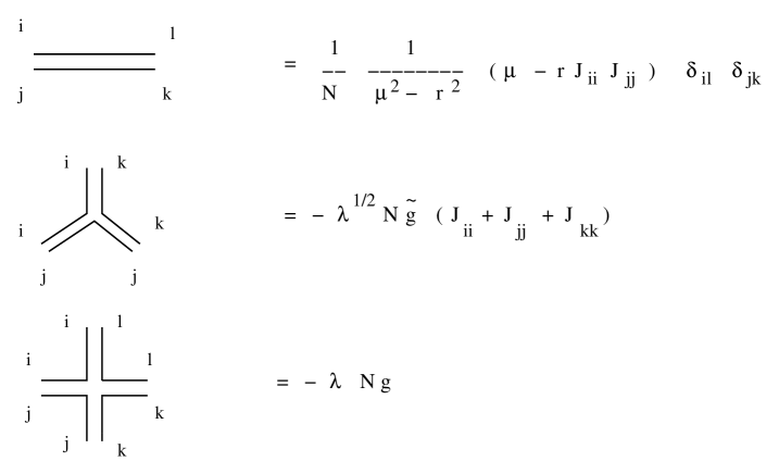
Figure 10: The Feynman rules for the $\lambda$-expansion of (C.1).

C.1 Full propagator, tadpole and 2PI vacuum diagrams

As the fundamental quantities in the present calculation, we consider the full propagator (the connected two-point function) and the tadpole (the one-point function), which can be written respectively as

$$\langle\phi_{ij}\phi_{kl}\rangle_{\rm C} \equiv \langle\phi_{ij}\phi_{kl}\rangle-\langle\phi_{ij}\rangle\langle\phi_{kl}\rangle=\frac{1}{N}(c+dJ_{ii}J_{jj})\delta_{il}\delta_{jk}\ ,$$

$$\langle\phi_{ij}\rangle = \sqrt{\lambda}\,TJ_{ii}\delta_{ij}$$ (C.2)

due to the SU($N/2$)$\times$SU($N/2$) symmetry. At the leading order, $c$, $d$ and $T$ are given by

$$c=\frac{\mu}{\mu^{2}-r^{2}}+O(\lambda)\ ,\qquad d=\frac{-r}{\mu^{2}-r^{2}}+O(\lambda)\ ,\qquad T=-\tilde{g}\frac{1}{\mu+r}\frac{2\mu-r}{\mu^{2}-r^{2}}+O(\lambda)\ .$$ (C.3)

In what follows we will use the Schwinger-Dyson equations for the full propagator and the tadpole to reduce the calculation of the free energy to that of two-particle-irreducible (2PI) planar vacuum diagrams. By ‘two-particle-irreducible’ we mean that the diagram cannot be separated into two parts by removing two propagators. For later convenience we use the full propagator for internal lines, and denote the sum of those diagrams as $N^{2}G(c,d)$. For example $N^{2}G(c,d)$ consists of 5 diagrams shown in Fig. 11 up to the 2nd order, and the results of the first two diagrams are given by $\frac{1}{2}\lambda\tilde{g}^{2}N^{2}(c^{3}+d^{3}+2c^{2}d+2cd^{2})$ and $-\frac{1}{2}\lambda gN^{2}c^{2}$ respectively. The important point is that there are much less two-particle-irreducible (2PI) vacuum diagrams than general vacuum diagrams that need to be considered in order to obtain the free energy ${\cal F}(\mu,r)$ directly.

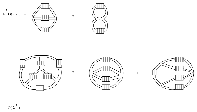
Figure 11: The 2PI planar vacuum diagrams up to $O(\lambda^{2})$. The internal line with the rectangular blob stands for the full propagator. The two diagrams in the first line are of $O(\lambda)$, while the three diagrams in the second line are of $O(\lambda^{2})$.

C.2 Derivation of the Schwinger-Dyson equations

Here we will derive the Schwinger-Dyson equations, which allow us to obtain the full propagator and the tadpole order by order in $\lambda$.

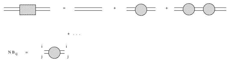
Figure 12: The full propagator can be expressed as a geometric series. The round blob represents the radiative correction to the quadratic term, which is denoted by $NB_{ij}$ as indicated in the second line.

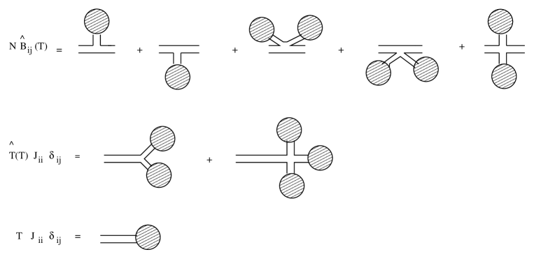
Figure 13: The first two lines show the diagrams which contribute to the parts of $B_{ij}$ and $T$ which depend only on $T$ but not on $c$ or $d$. The round blob attached at the ends of the double-line represents the tadpole $TJ_{ii}\delta_{ij}$ as stated in the last line.

Figure 14: The full result for $\hat{B}_{ij}(c,d,T)$ can be obtained from $\hat{B}_{ij}(c,d,T=0)$ by dressing the 3-point vertices with the tadpole.

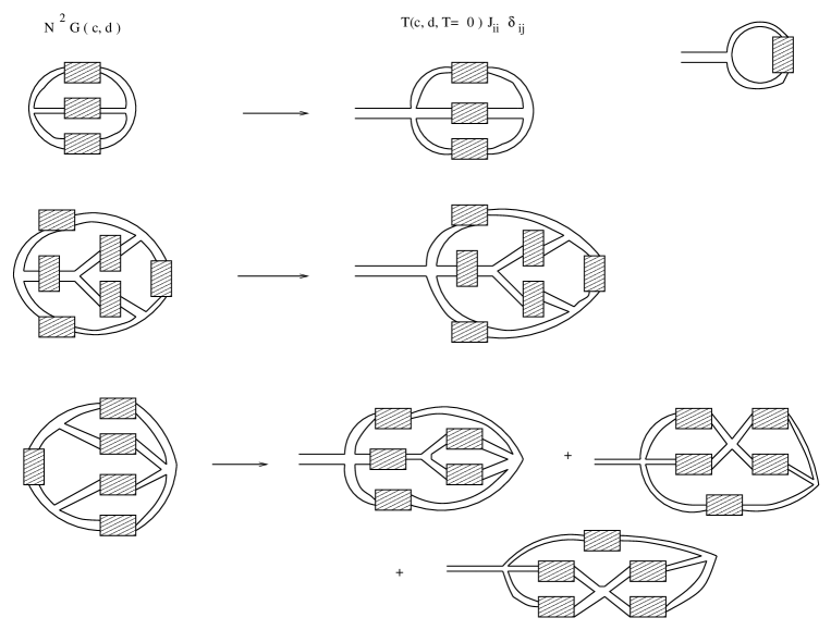
Figure 15: Except for the lowest order diagram shown in the upper right corner, all the diagrams contributing to $\hat{T}(c,d,T=0)$ are obtained by attaching an external line to a 3-point vertex in the diagrams contributing to $N^{2}G(c,d)$. The diagrams at the first few orders are shown for illustration.

Let us note first that the full propagator can be expressed as a geometric series as depicted in Fig. 12. The round blob, which we denote as $NB_{ij}$, stands for the radiative correction to the quadratic term. One can solve this relation for $B_{ij}$ as

$$B_{ij}=\mu-\frac{c}{c^{2}-d^{2}}+\left(r+\frac{d}{c^{2}-d^{2}}\right)J_{ii}J_{jj}\ .$$ (C.4)

It is convenient to decompose $B_{ij}$ as

$$B_{ij}=\hat{B}_{ij}(T)+\hat{B}_{ij}(c,d,T)\ ,$$ (C.5)

where $\hat{B}_{ij}(T)$ contains only tadpoles and hence do not depend on $c$ or $d$. One can easily see that $\hat{B}_{ij}(T)$ consists of 5 diagrams shown in Fig. 13, which yield

$$\hat{B}_{ij}(T)=(-2\lambda\tilde{g}T-\lambda^{2}gT^{2})(2+J_{ii}J_{jj})\ .$$ (C.6)

The second term in (C.5) can be obtained from the sum of 2PI diagrams $G(c,d)$ as follows. Note first that $\hat{B}_{ij}(c,d,T=0)$ can be obtained from $G(c,d)$ by removing one full propagator, i.e.,

$$\hat{B}_{ij}(c,d,T=0)=2\frac{\partial}{\partial c}G(c,d)+2\frac{\partial}{\partial d}G(c,d)J_{ii}J_{jj}\ .$$ (C.7)

Then one can obtain $\hat{B}_{ij}(c,d,T)$ for $T\neq 0$ by the shifting the three-point vertex as (See Fig. 14)

$$\hat{B}_{ij}(c,d,T)=\left.\hat{B}_{ij}(c,d,T=0)\right|_{\tilde{g}\rightarrow\tilde{g}+\lambda gT}\ .$$ (C.8)

Summation of (C.6) and (C.8) yields

$$B_{ij}=\left[2\frac{\partial}{\partial c}G(c,d)+2\frac{\partial}{\partial d}G(c,d)J_{ii}J_{jj}\right]_{\tilde{g}\rightarrow\tilde{g}+\lambda gT}-(2\lambda\tilde{g}T+\lambda^{2}gT^{2})(2+J_{ii}J_{jj})\ .$$ (C.9)

From (C.4) and (C.9) we obtain the Schwinger-Dyson equations for the full propagator

$$\mu-\frac{c}{c^{2}-d^{2}}=\left[2\frac{\partial}{\partial c}G(c,d)\right]_{\tilde{g}\rightarrow\tilde{g}+\lambda gT}-2(2\lambda\tilde{g}T+\lambda^{2}gT^{2})\ ,$$

$$r+\frac{d}{c^{2}-d^{2}}=\left[2\frac{\partial}{\partial d}G(c,d)\right]_{\tilde{g}\rightarrow\tilde{g}+\lambda gT}-(2\lambda\tilde{g}T+\lambda^{2}gT^{2})\ .$$ (C.10)

The Schwinger-Dyson equation for the tadpole can be obtained in a similar way. Let us first decompose the tadpole $T$ as

$$T=\hat{T}(T)+\hat{T}(c,d,T)\ .$$ (C.11)

The first term, which includes only tadpoles, consists of two diagrams shown in Fig. 13, which yield

$$\hat{T}(T)=\frac{1}{\mu+r}(-3\lambda\tilde{g}T^{2}-\lambda^{2}gT^{3})\ .$$ (C.12)

Next we consider the diagrams that contribute to $\hat{T}(c,d,T=0)$. Note that every diagram other than the one at the lowest order can be obtained from 2PI vacuum diagrams by attaching an external line to a 3-point vertex as illustrated in Fig. 15. Thus we have

$$\hat{T}(c,d,T=0)=-\tilde{g}\frac{1}{\mu+r}(2c+d)+g\frac{1}{\mu+r}\frac{\partial}{\partial\tilde{g}}G(c,d)\ ,$$ (C.13)

where the first term represents the contribution from the lowest order diagram. Then $\hat{T}(c,d,T)$ with $T\neq 0$ can be obtained from $\hat{T}(c,d,T=0)$ by the same replacement as in Fig. 14, which leads us to

$$\hat{T}(c,d,T)=\left.\frac{1}{\mu+r}\left[-\tilde{g}(2c+d)+g\frac{\partial}{\partial\tilde{g}}G(c,d)\right]\right|_{\tilde{g}\rightarrow\tilde{g}+\lambda gT}.$$ (C.14)

From (C.11), (C.12) and (C.14), we obtain the Schwinger-Dyson equation for the tadpole

$$T=\left.\frac{1}{\mu+r}\left[-\tilde{g}(2c+d)+g\frac{\partial}{\partial\tilde{g}}G(c,d)\right]\right|_{\tilde{g}\rightarrow\tilde{g}+\lambda gT}-\frac{1}{\mu+r}(3\lambda\tilde{g}T^{2}+\lambda^{2}gT^{3})\ .$$ (C.15)

Since Eqs. (C.10) and (C.15) are closed with respect to $c$, $d$, $T$, we can solve them order by order once the sum of 2PI diagrams $G(c,d)$ is obtained.

C.3 Explicit form of the free energy

From the full propagator and the tadpole, one can readily obtain the expectation value of the quadratic terms in (C.1) as

$${\cal M}\equiv\left\langle\frac{1}{N}{\rm tr\,}\phi^{2}\right\rangle=c+\lambda T^{2},\qquad{\cal M}_{J}\equiv\left\langle\frac{1}{N}{\rm tr\,}(J\phi J\phi)\right\rangle=d+\lambda T^{2}.$$ (C.16)

Since the free energy ${\cal F}(\mu,r)$ satisfies the differential equations

$$4\frac{\partial}{\partial\mu_{+}}{\cal F}(\mu,r)={\cal M}+{\cal M}_{J}~{}~{}~{},~{}~{}~{}\qquad 4\frac{\partial}{\partial\mu_{-}}{\cal F}(\mu,r)={\cal M}-{\cal M}_{J}\ ,$$ (C.17)

where $\mu_{\pm}=\mu\pm r$, we can obtain the $\lambda$-expansion of the free energy by term-by-term integration. The integration constant in ${\cal F}(\mu,r)$, which does not depend on $\mu_{\pm}$, appears only at the order of $O(\lambda^{0})$, and it can be calculated directly as $\frac{1}{2}(\ln N-\ln 2)$.

The number of 2PI planar vacuum diagrams up to the 3rd order is 13. By evaluating them explicitly and by following the above procedure we obtain the explicit form of the free energy ${\cal F}(\mu,r)$ up to the 3rd order as follows.

$${\cal F}(\mu,r) = \sum_{n=0}^{\infty}\lambda^{n}{\cal F}_{n}(\mu,r),$$ (C.18)

$${\cal F}_{0}(\mu,r) = \frac{1}{4}\Bigl{[}2\ln N+\ln(\mu_{+}\mu_{-})-2\ln 2\Bigr{]},$$

$${\cal F}_{1}(\mu,r) = \frac{\tilde{g}^{2}}{4}\left(-\frac{6}{\mu_{+}^{3}}-\frac{3}{\mu_{+}^{2}\mu_{-}}-\frac{1}{\mu_{+}\mu_{-}^{2}}\right)+\frac{g}{4}\left(\frac{1}{2\mu_{+}^{2}}+\frac{1}{\mu_{+}\mu_{-}}+\frac{1}{2\mu_{-}^{2}}\right),$$

$${\cal F}_{2}(\mu,r) = \frac{\tilde{g}^{4}}{4}\left(-\frac{108}{\mu_{+}^{6}}-\frac{54}{\mu_{+}^{5}\mu_{-}}-\frac{81}{4\mu_{+}^{4}\mu_{-}^{2}}-\frac{17}{2\mu_{+}^{3}\mu_{-}^{3}}-\frac{9}{4\mu_{+}^{2}\mu_{-}^{4}}\right)$$

$$+\frac{g\tilde{g}^{2}}{4}\left(\frac{27}{\mu_{+}^{5}}+\frac{99}{4\mu_{+}^{4}\mu_{-}}+\frac{47}{4\mu_{+}^{3}\mu_{-}^{2}}+\frac{25}{4\mu_{+}^{2}\mu_{-}^{3}}+\frac{9}{4\mu_{+}\mu_{-}^{4}}\right)$$

$$+\frac{g^{2}}{4}\left(-\frac{9}{16\mu_{+}^{4}}-\frac{1}{\mu_{+}^{3}\mu_{-}}-\frac{11}{8\mu_{+}^{2}\mu_{-}^{2}}-\frac{1}{\mu_{+}\mu_{-}^{3}}-\frac{9}{16\mu_{-}^{4}}\right),$$

$${\cal F}_{3}(\mu,r) = \frac{\tilde{g}^{6}}{4}\left(-\frac{3402}{\mu_{+}^{9}}-\frac{1944}{\mu_{+}^{8}\mu_{-}}-\frac{810}{\mu_{+}^{7}\mu_{-}^{2}}-\frac{351}{\mu_{+}^{6}\mu_{-}^{3}}-\frac{135}{\mu_{+}^{5}\mu_{-}^{4}}-\frac{45}{\mu_{+}^{4}\mu_{-}^{5}}-\frac{9}{\mu_{+}^{3}\mu_{-}^{6}}\right)$$

$$+\frac{g\tilde{g}^{4}}{4}\left(\frac{1377}{\mu_{+}^{8}}+\frac{1188}{\mu_{+}^{7}\mu_{-}}+\frac{1215}{2\mu_{+}^{6}\mu_{-}^{2}}+\frac{306}{\mu_{+}^{5}\mu_{-}^{3}}+\frac{135}{\mu_{+}^{4}\mu_{-}^{4}}+\frac{54}{\mu_{+}^{3}\mu_{-}^{5}}+\frac{27}{2\mu_{+}^{2}\mu_{-}^{6}}\right)$$

$$+\frac{g^{2}\tilde{g}^{2}}{4}\left(-\frac{243}{2\mu_{+}^{7}}-\frac{621}{4\mu_{+}^{6}\mu_{-}}-\frac{477}{4\mu_{+}^{5}\mu_{-}^{2}}-\frac{153}{2\mu_{+}^{4}\mu_{-}^{3}}-\frac{81}{2\mu_{+}^{3}\mu_{-}^{4}}-\frac{81}{4\mu_{+}^{2}\mu_{-}^{5}}-\frac{27}{4\mu_{+}\mu_{-}^{6}}\right)$$

$$+\frac{g^{3}}{4}\left(\frac{9}{8\mu_{+}^{6}}+\frac{9}{4\mu_{+}^{5}\mu_{-}}+\frac{27}{8\mu_{+}^{4}\mu_{-}^{2}}+\frac{9}{2\mu_{+}^{3}\mu_{-}^{3}}+\frac{27}{8\mu_{+}^{2}\mu_{-}^{4}}+\frac{9}{4\mu_{+}\mu_{-}^{5}}+\frac{9}{8\mu_{-}^{6}}\right)\ .$$

References

- [1] W. E. Caswell, Accurate Energy Levels For The Anharmonic Oscillator And A Summable Series For The Double Well Potential In Perturbation Theory, Annals Phys. 123 (1979) 153; I. G. Halliday and P. Suranyi, The Anharmonic Oscillator: A New Approach, Phys. Rev. D 21 (1980) 1529; J. Killingbeck, Renormalised Perturbation Series, J. Phys. A 14 (1981) 1005.
- [2] P. M. Stevenson, Optimized Perturbation Theory, Phys. Rev. D 23 (1981) 2916 .
- [3] P. M. Stevenson, Optimization And The Ultimate Convergence Of QCD Perturbation Theory, Nucl. Phys. B 231 (1984) 65; I. R. Buckley, A. Duncan and H. F. Jones, Proof Of The Convergence Of The Linear Delta Expansion, Phys. Rev. D 47 (1993) 2554; A. Duncan and H. F. Jones, Convergence proof for optimized Delta expansion: The Anharmonic oscillator, ibid. (1993) 2560; C. M. Bender, A. Duncan and H. F. Jones, Convergence of the optimized delta expansion for the connected vacuum amplitude: Zero dimensions, Phys. Rev. D 49 (1994) 4219 [hep-th/9310031]; R. Guida, K. Konishi and H. Suzuki, Convergence of scaled delta expansion: Anharmonic oscillator, Annals Phys. 241 (1995) 152 [hep-th/9407027]; Improved convergence proof of the delta expansion and order dependent mappings, ibid. 249 (1996) 109 [hep-th/9505084].
- [4] A. Okopinska, Nonstandard Expansion Techniques For The Effective Potential In Quantum Field Theory, Phys. Rev. D 35 (1987) 1835; Optimized Expansion In Quantum Field Theory Of Massive Fermions With Interaction, Phys. Rev. D 38 (1988) 2507; I. Stancu and P. M. Stevenson, Second Order Corrections to the Gaussian Effective Potential of Theory, Phys. Rev. D 42 (1990) 2710; E. Braaten and E. Radescu, Convergence of the linear delta expansion in the critical O(N) field theory, [hep-ph/0206108].
- [5] A. Dhar, Renormalization Scheme - Invariant Perturbation Theory, Phys. Lett. B 128 (1983) 407.
- [6] S. Kawamoto and T. Matsuo, Improved renormalization group analysis for Yang-Mills theory, [hep-th/0307171].
- [7] D. Kabat and G. Lifschytz, Approximations for strongly-coupled supersymmetric quantum mechanics, Nucl. Phys. B 571 (2000) 419 [hep-th/9910001].
- [8] T. Banks, W. Fischler, S. H. Shenker and L. Susskind, M theory as a matrix model: A conjecture, Phys. Rev. D 55 (1997) 5112 [hep-th/9610043].
- [9] D. Kabat, G. Lifschytz and D.A. Lowe, Black hole thermodynamics from calculations in strongly-coupled gauge theory, Phys. Rev. Lett. 86 (2001) 1426 [hep-th/0007051]; Black hole entropy from non-perturbative gauge theory, Phys. Rev. D 64 (2001) 124015 [hep-th/0105171]; N. Iizuka, D. Kabat, G. Lifschytz and D. A. Lowe, Probing black holes in non-perturbative gauge theory, Phys. Rev. D 65 (2002) 024012 [hep-th/0108006].
- [10] M. Engelhardt and S. Levit, Variational master field for large-N interacting matrix models: Free random variables on trial, Nucl. Phys. B 488 (1997) 735 [hep-th/9609216].
- [11] J. Nishimura and F. Sugino, Dynamical generation of four-dimensional space-time in the IIB matrix model, JHEP 0205 (2002) 001 [hep-th/0111102].
- [12] N. Ishibashi, H. Kawai, Y. Kitazawa and A. Tsuchiya, A Large- Reduced Model as Superstring, Nucl. Phys. B 498 (1997) 467 [hep-th/9612115].
- [13] P. Austing and J.F. Wheater, The convergence of Yang-Mills integrals, JHEP 0102 (2001) 028 [hep-th/0101071]; Convergent Yang-Mills matrix theories, JHEP 0104 (2001) 019 [hep-th/0103159].
- [14] T. Hotta, J. Nishimura and A. Tsuchiya, Dynamical Aspects of Large Reduced Models, Nucl. Phys. B 545 (1999) 543 [hep-th/9811220].
- [15] W. Krauth, H. Nicolai and M. Staudacher, Monte Carlo approach to M-theory, Phys. Lett. B 431 (1998) 31 [hep-th/9803117]; W. Krauth and M. Staudacher, Finite Yang-Mills integrals, Phys. Lett. B 435 (1998) 350 [hep-th/9804199]; J. Ambjørn, K.N. Anagnostopoulos, W. Bietenholz, T. Hotta and J. Nishimura, Large Dynamics of Dimensionally Reduced 4D SU() Super Yang-Mills Theory, JHEP 0007 (2000) 013 [hep-th/0003208]; J. Ambjørn, K.N. Anagnostopoulos, W. Bietenholz, T. Hotta and J. Nishimura, Monte Carlo Studies of the IIB Matrix Model at Large , JHEP 0007 (2000) 011 [hep-th/0005147]; P. Bialas, Z. Burda, B. Petersson and J. Tabaczek, Large Limit of the IKKT Model, Nucl. Phys. B 592 (2001) 391 [hep-lat/0007013]; Z. Burda, B. Petersson and J. Tabaczek, Geometry of Reduced Supersymmetric 4D Yang-Mills Integrals, Nucl. Phys. B 602 (2001) 399 [hep-lat/0012001]; J. Ambjørn, K.N. Anagnostopoulos, W. Bietenholz, F. Hofheinz and J. Nishimura, On the Spontaneous Breakdown of Lorentz Symmetry in Matrix Models of Superstrings, Phys. Rev. D 65 (2002) 086001 [hep-th/0104260]; K.N. Anagnostopoulos, W. Bietenholz and J. Nishimura, The Area Law in Matrix Models for Large QCD Strings, Int. J. Mod. Phys. C 13 (2002) 555 [hep-lat/0112035].
- [16] S. Oda and F. Sugino, Gaussian and mean field approximations for reduced Yang-Mills integrals, JHEP 0103 (2001) 026 [hep-th/0011175]; F. Sugino, Gaussian and mean field approximations for reduced 4D supersymmetric Yang-Mills integral, JHEP 0107 (2001) 014 [hep-th/0105284].
- [17] H. Aoki, S. Iso, H. Kawai, Y. Kitazawa and T. Tada, Space-time structures from IIB matrix model, Prog. Theor. Phys. 99 (1998) 713 [hep-th/9802085].
- [18] J. Nishimura and G. Vernizzi, Spontaneous Breakdown of Lorentz Invariance in IIB Matrix Model, JHEP 0004 (2000) 015 [hep-th/0003223]; Brane World Generated Dynamically from String Type IIB Matrices, Phys. Rev. Lett. 85 (2000) 4664 [hep-th/0007022]; J. Nishimura, Exactly solvable matrix models for the dynamical generation of space-time in superstring theory, Phys. Rev. D 65 (2002) 105012 [hep-th/0108070].
- [19] K. N. Anagnostopoulos and J. Nishimura, New approach to the complex-action problem and its application to a nonperturbative study of superstring theory, Phys. Rev. D 66 (2002) 106008 [hep-th/0108041].
- [20] G. Vernizzi and J. F. Wheater, Rotational symmetry breaking in multi-matrix models, Phys. Rev. D 66 (2002) 085024 [hep-th/0206226].
- [21] T. Imai, Y. Kitazawa, Y. Takayama and D. Tomino, Effective actions of matrix models on homogeneous spaces, [hep-th/0307007].
- [22] H. Kawai, S. Kawamoto, T. Kuroki, T. Matsuo and S. Shinohara, Mean field approximation of IIB matrix model and emergence of four dimensional space-time, Nucl. Phys. B 647 (2002) 153 [hep-th/0204240].
- [23] H. Kawai, S. Kawamoto, T. Kuroki and S. Shinohara, Improved perturbation theory and four-dimensional space-time in IIB matrix model, Prog. Theor. Phys. 109 (2003) 115 [hep-th/0211272].
- [24] J. Nishimura, T. Okubo and F. Sugino, Convergence of the Gaussian expansion method in dimensionally reduced Yang-Mills integrals, JHEP 0210 (2002) 043 [hep-th/0205253].
- [25] E. Brezin, C. Itzykson, G. Parisi and J. B. Zuber, Planar Diagrams, Commun. Math. Phys. 59 (1978) 35.
- [26] G. M. Cicuta, L. Molinari and E. Montaldi, Large N Phase Transitions In Low Dimensions, Mod. Phys. Lett. A 1 (1986) 125.