UMTG–243

Finite size effects in the XXZ and sine-Gordon models
with two boundaries
Changrim Ahn and Rafael I. Nepomechie

We compute the boundary energy and the Casimir energy for both the spin-${1\over 2}$ XXZ quantum spin chain and (by means of the light-cone lattice construction) the massive sine-Gordon model with both left and right boundaries. We also derive a nonlinear integral equation for the ground state of the sine-Gordon model on a finite interval. These results, which are based on a recently-proposed Bethe Ansatz solution, are for general values of the bulk coupling constant, and for both diagonal and nondiagonal boundary interactions. However, the boundary parameters are restricted to obey one complex (two real) constraints.

1 Introduction

The spin-${1\over 2}$ XXZ quantum spin chain and the sine-Gordon quantum field theory on a finite interval (i.e., with both left and right boundaries) have applications in statistical mechanics, condensed matter physics and string theory, and have therefore been studied intensively, e.g., [1] - [15]. Much of this work has been restricted to either diagonal boundary interactions [1] - [4], [7] - [10] or to special values of the bulk coupling constant [13, 14, 15], because a solution of the XXZ chain with general (both diagonal and nondiagonal) boundary terms [5] has not been available. A solution of the latter problem for values of the boundary parameters obeying a linear constraint has recently been proposed [16, 17, 18] and confirmed numerically [19].

We exploit here this new solution to compute finite-size corrections to the ground-state energy of both the XXZ chain and (by means of the light-cone lattice approach [20, 21, 22]) the massive sine-Gordon model, in a range of parameter space heretofore not possible. In particular, we compute the boundary energy and Casimir energy, and we derive a Klümper - Pearce - Destri - de Vega [23, 24] nonlinear integral equation for the ground state of the sine-Gordon model on a finite interval.

The outline of this article is as follows. In Section 2, we consider the open XXZ quantum spin chain with $N$ spins. After a brief review of the Bethe Ansatz solution [16, 17, 18], we compute the ground-state energy, in particular the corrections of order $1$ and $1/N$, and therefore [26, 27], the central charge. In Section 3, we turn to the sine-Gordon model on an interval of length $R$. We observe that this model contains an additional boundary parameter $|\gamma_{+}-\gamma_{-}|$ which has not previously been noted. We analyze the light-cone lattice [9, 20, 21, 22] version of this model, which is formally quite similar to the open XXZ chain. We determine the relation between the lattice and continuum boundary parameters by matching the boundary (order $1$) energies in the corresponding models. We then formulate a nonlinear integral equation [23, 24] for the ground state, and give a corresponding formula for the Casimir (order $1/R$) energy. In the ultraviolet $(R\rightarrow 0$) limit, the central charge of the sine-Gordon model coincides with that of the XXZ spin chain. Our result for the Casimir energy at the free-Fermion point coincides with the result from the TBA approach of Caux et al. [15]. Moreover, we compute the Casimir energy numerically over a wide range of bulk and boundary parameters, and track the crossover from the ultraviolet to the infrared regions. We conclude in Section 4 with a brief discussion of our results and some interesting open problems.

2 The open XXZ quantum spin chain

We begin by briefly reviewing the recently-proposed [16, 17, 18] Bethe Ansatz solution of the open spin-${1\over 2}$ XXZ quantum spin chain with both diagonal and nondiagonal boundary terms. In terms of the parameters introduced in the latter reference, the Hamiltonian is given by

$${\cal H} = {1\over 2}\Big{\{}\sum_{n=1}^{N-1}\left(\sigma_{n}^{x}\sigma_{n+1}^{x}+\sigma_{n}^{y}\sigma_{n+1}^{y}+\cosh\eta\ \sigma_{n}^{z}\sigma_{n+1}^{z}\right)$$ (2.1)

$$+ \sinh\eta\Big{[}\coth\alpha_{-}\tanh\beta_{-}\sigma_{1}^{z}+\mathop{\rm csch}\nolimits\alpha_{-}\mathop{\rm sech}\nolimits\beta_{-}\big{(}\cosh\theta_{-}\sigma_{1}^{x}+i\sinh\theta_{-}\sigma_{1}^{y}\big{)}$$

$$- \coth\alpha_{+}\tanh\beta_{+}\sigma_{N}^{z}+\mathop{\rm csch}\nolimits\alpha_{+}\mathop{\rm sech}\nolimits\beta_{+}\big{(}\cosh\theta_{+}\sigma_{N}^{x}+i\sinh\theta_{+}\sigma_{N}^{y}\big{)}\Big{]}\Big{\}}\,,$$

where $\sigma^{x}\,,\sigma^{y}\,,\sigma^{z}$ are the usual Pauli matrices, $\eta$ is the bulk anisotropy parameter, $\alpha_{\pm}\,,\beta_{\pm}\,,\theta_{\pm}$ are boundary parameters, and $N$ is the number of spins. The boundary parameters are assumed to satisfy the linear constraint

$$\alpha_{-}+\beta_{-}+\alpha_{+}+\beta_{+}=\pm(\theta_{-}-\theta_{+})+\eta k\,,$$ (2.2)

where $k$ is an even integer if $N$ is odd, and is an odd integer if $N$ is even. In terms of the “shifted” Bethe roots $\{\tilde{u}_{j}\}$ [19], the energy eigenvalues are given by

$$E = \sinh^{2}\eta\sum_{j=1}^{M}{1\over\sinh(\tilde{u}_{j}-{\eta\over 2})\ \sinh(\tilde{u}_{j}+{\eta\over 2})}+{1\over 2}\sinh\eta\left(\coth\alpha_{-}+\tanh\beta_{-}+\coth\alpha_{+}+\tanh\beta_{+}\right)$$ (2.3)

$$+ {1\over 2}(N-1)\cosh\eta\,,$$

and the Bethe Ansatz equations are given by

$$\left({\sinh(\tilde{u}_{j}+{\eta\over 2})\over\sinh(\tilde{u}_{j}-{\eta\over 2})}\right)^{2N}{\sinh(\tilde{2}u_{j}+\eta)\over\sinh(\tilde{2}u_{j}-\eta)}{\sinh(\tilde{u}_{j}-{\eta\over 2}+\alpha_{-})\over\sinh(\tilde{u}_{j}+{\eta\over 2}-\alpha_{-})}{\cosh(\tilde{u}_{j}-{\eta\over 2}+\beta_{-})\over\cosh(\tilde{u}_{j}+{\eta\over 2}-\beta_{-})}$$ (2.4)

$$\times{\sinh(\tilde{u}_{j}-{\eta\over 2}+\alpha_{+})\over\sinh(\tilde{u}_{j}+{\eta\over 2}-\alpha_{+})}{\cosh(\tilde{u}_{j}-{\eta\over 2}+\beta_{+})\over\cosh(\tilde{u}_{j}+{\eta\over 2}-\beta_{+})}=-\prod_{k=1}^{M}{\sinh(\tilde{u}_{j}-\tilde{u}_{k}+\eta)\over\sinh(\tilde{u}_{j}-\tilde{u}_{k}-\eta)}{\sinh(\tilde{u}_{j}+\tilde{u}_{k}+\eta)\over\sinh(\tilde{u}_{j}+\tilde{u}_{k}-\eta)}\,,$$

$$j=1\,,\cdots\,,M\,,$$

where the number $M$ of Bethe roots is given by

$$M={1\over 2}(N-1+k)\,,$$ (2.5)

$k$ being the integer appearing in (2.2). The case of diagonal boundary terms [2, 4] corresponds to the limit $\beta_{\pm}\rightarrow\pm\infty$, in which case the constraint (2.2) disappears.

We restrict our attention here to the “massless” regime (bulk anisotropy parameter $\eta$ purely imaginary, with $0<\Im m\ \eta<\pi$); and therefore, to ensure Hermiticity of the Hamiltonian (2.1), we restrict the boundary parameters $\alpha_{\pm}\,,\theta_{\pm}$ to be purely imaginary, and $\beta_{\pm}$ to be purely real. It is convenient to define new bulk and boundary parameters,

$$\eta=i\mu\,,\qquad\alpha_{\pm}=i\mu a_{\pm}\,,\qquad\beta_{\pm}=\mu b_{\pm}\,,\qquad\theta_{\pm}=i\mu c_{\pm}\,,$$ (2.6)

where $\mu\,,a_{\pm}\,,b_{\pm}\,,c_{\pm}$ are all real, with $0<\mu<\pi$. We use the periodicity $\alpha_{\pm}\mapsto\alpha_{\pm}+2\pi i$ of the Hamiltonian (2.1) (and in fact, of the full transfer matrix) to restrict $\alpha_{\pm}$ to the fundamental domain $-\pi+{\mu\over 2}<\Im m\ \alpha_{\pm}<\pi+{\mu\over 2}$, which implies

$${1\over 2}-\nu<a_{\pm}<{1\over 2}+\nu\,,$$ (2.7)

where $\nu\equiv{\pi\over\mu}>1$.

Considering separately the imaginary and real parts of the constraint equation (2.2), we see that the boundary parameters must in fact satisfy a pair of real constraints

$$a_{-}+a_{+} = \pm|c_{-}-c_{+}|+k\,,$$

$$b_{-}+b_{+} = 0\,.$$ (2.8)

The absolute values can be introduced without loss of generality, since the preceding sign is arbitrary.

The energy eigenvalues $E$ depend on the parameters $c_{\pm}$ only through the absolute value of their difference, $|c_{-}-c_{+}|$. Indeed, by performing on the Hamiltonian (2.1) a global spin rotation about the $z$ axis, the parameters $c_{\pm}$ are shifted by a constant, i.e., $c_{\pm}\mapsto c_{\pm}+const$. In particular, one can eliminate one of these two parameters (say, $c_{+}$), which results in a shift of the other ($c_{-}\mapsto c_{-}-c_{+}$). Hence, the energy depends on the difference $c_{-}-c_{+}$. Furthermore, by performing on the Hamiltonian a time-reversal (complex-conjugation) transformation, the parameters $c_{\pm}$ are negated, i.e., $c_{\pm}\mapsto-c_{\pm}$. Hence, the energy in fact depends on $|c_{-}-c_{+}|$.

Let us consider the energy of the ground state of this model as a function of $N$, for large $N$. The leading (order $N$) contribution, which does not depend on the boundary interactions, is well known [28]. Our objective here is to compute the boundary (order $1$) and Casimir (order $1/N$) corrections.

2.1 Boundary energy

Let us streamline the notation by defining the basic quantities

$$e_{n}(\lambda)={\sinh\mu\left(\lambda+{in\over 2}\right)\over\sinh\mu\left(\lambda-{in\over 2}\right)}\,,\qquad g_{n}(\lambda)=e_{n}(\lambda\pm{i\pi\over 2\mu})={\cosh\mu\left(\lambda+{in\over 2}\right)\over\cosh\mu\left(\lambda-{in\over 2}\right)}\,.$$ (2.9)

The Bethe Ansatz Eqs. (2.4) then take the compact form

$$e_{1}(\lambda_{j})^{2N+1}\ g_{1}(\lambda_{j}){e_{2a_{-}-1}(\lambda_{j})\ e_{2a_{+}-1}(\lambda_{j})\over g_{1+2ib_{-}}(\lambda_{j})\ g_{1+2ib_{+}}(\lambda_{j})} = -\prod_{k=1}^{M}e_{2}(\lambda_{j}-\lambda_{k})\ e_{2}(\lambda_{j}+\lambda_{k})\,,$$ (2.10)

$$j=1\,,\cdots\,,M\,,$$

where we have set $\tilde{u}_{j}=\mu\lambda_{j}$, and we use the new parameters introduced in (2.6).

We wish to focus here on the ground state with no holes. Hence, we take $N$ even, since states with $N$ odd correspond to excited states with an odd number of holes. Moreover, we take (see Eq. (2.5))

$$k=1\,,\qquad M={N\over 2}\,.$$ (2.11)

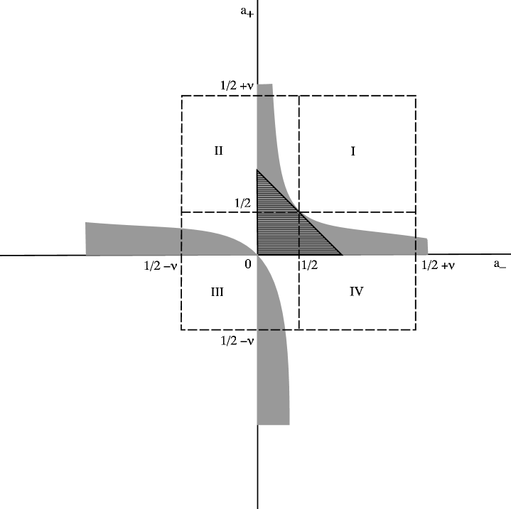
Figure 1: Domain of boundary parameters $a_{\pm}$. For the ruled triangular region, the Bethe Ansatz does not give the ground state. For the shaded regions (including the special case noted in [19] corresponding to the line $a_{+}+a_{-}=1$), the Bethe Ansatz does give the ground state, but the shifted Bethe roots are not all real. For the blank regions (in particular, those labeled I - IV, as in Eq. (2.16)) the Bethe Ansatz gives the ground state, and all roots are real. (Based on numerical results for $N=4$, where $b_{\pm}$ and $c_{\pm}$ satisfy Eq. (2.8) with $k=1$. As $N$ increases, the shaded area also increases. We conjecture that for $N\rightarrow\infty$, only regions I - IV remain unshaded.)

According to [19], for this case the Bethe Ansatz solution correctly yields the energy of the ground state, and the shifted Bethe roots corresponding to this state are real. However, we have subsequently found through further numerical studies of chains with small values of $N$ that this statement must be qualified: there are regions in the parameter space (2.7) for which some of the shifted Bethe roots are imaginary (presumably corresponding to boundary bound states), or for which the Bethe Ansatz does not yield the ground state. (See Figure 1.) For simplicity, we henceforth restrict the boundary parameters $a_{\pm}$ to the following four regions,

$$\begin{array}[]{r@{\ : \quad}l}I&{1\over 2}<a_{\pm}<{1\over 2}+\nu\\ II&{1\over 2}<a_{+}<{1\over 2}+\nu\quad\&\quad{1\over 2}-\nu<a_{-}<0\\ III&{1\over 2}-\nu<a_{\pm}<0\\ IV&{1\over 2}-\nu<a_{+}<0\quad\&\quad{1\over 2}<a_{-}<{1\over 2}+\nu\end{array}$$ (2.16)

for which our numerical results indicate that the Bethe Ansatz solution does yield the energy of the ground state, and the shifted Bethe roots corresponding to this state are all real.

We remark that (2.7) implies that $-2\nu<a_{-}+a_{+}-1<2\nu$; and hence the first constraint in Eq. (2.8) with $k=1$ implies

$$|c_{-}-c_{+}|<2\nu\,.$$ (2.17)

This condition can always be satisfied, since the Hamiltonian and transfer matrix also have the periodicity $\theta_{\pm}\mapsto\theta_{\pm}+2\pi i$, which corresponds to $c_{\pm}\mapsto c_{\pm}+2\nu$.

In order to compute the energy of the ground state for large $N$, we first determine the density of (real) Bethe roots for this state. To this end, we take the logarithm of the Bethe Ansatz Eqs. (2.10) and obtain

$$h(\lambda_{j})=j\,,\qquad j=1\,,\cdots\,,{N\over 2}\,,$$ (2.18)

where the counting function $h(\lambda)$ is given by

$$h(\lambda) = {1\over 2\pi}\Big{\{}(2N+1)q_{1}(\lambda)+r_{1}(\lambda)+q_{2a_{-}-1}(\lambda)-r_{1+2ib_{-}}(\lambda)+q_{2a_{+}-1}(\lambda)-r_{1+2ib_{+}}(\lambda)$$ (2.19)

$$- \sum_{k=1}^{N\over 2}\left[q_{2}(\lambda-\lambda_{k})+q_{2}(\lambda+\lambda_{k})\right]\Big{\}}\,,$$

where $q_{n}(\lambda)$ and $r_{n}(\lambda)$ are odd functions defined by

$$q_{n}(\lambda) = \pi+i\ln e_{n}(\lambda)=2\tan^{-1}\left(\cot(n\mu/2)\tanh(\mu\lambda)\right)\,,$$

$$r_{n}(\lambda) = i\ln g_{n}(\lambda)\,.$$ (2.20)

We have checked numerically that, for the ground state, the right-hand-side of (2.18) is indeed given by successive integers from $1$ to $N/2$ [1, 2]. The Bethe roots $\{\lambda_{k}\}$ can all be chosen to be strictly positive. Then, defining $\lambda_{-k}\equiv-\lambda_{k}$, we rewrite the last term in (2.19) more symmetrically as follows:

$$-\sum_{k=1}^{N\over 2}\left[q_{2}(\lambda-\lambda_{k})+q_{2}(\lambda+\lambda_{k})\right]=-\sum_{k=-{N\over 2}}^{N\over 2}q_{2}(\lambda-\lambda_{k})+q_{2}(\lambda)\,.$$ (2.21)

The root density $\rho(\lambda)$ for the ground state is therefore given by

$$\rho(\lambda) = {1\over N}{dh\over d\lambda}$$

$$= 2a_{1}(\lambda)-\int_{-\infty}^{\infty}d\lambda^{\prime}\ a_{2}(\lambda-\lambda^{\prime})\ \rho(\lambda^{\prime})$$

$$+ {1\over N}\left[a_{1}(\lambda)+b_{1}(\lambda)+a_{2}(\lambda)+a_{2a_{-}-1}(\lambda)-b_{1+2ib_{-}}(\lambda)+a_{2a_{+}-1}(\lambda)-b_{1+2ib_{+}}(\lambda)\right]\,,$$

where we have ignored corrections of higher order in $1/N$ when passing from a sum to an integral, and we have introduced the notations

$$a_{n}(\lambda) = {1\over 2\pi}{d\over d\lambda}q_{n}(\lambda)={\mu\over\pi}{\sin(n\mu)\over\cosh(2\mu\lambda)-\cos(n\mu)}\,,$$

$$b_{n}(\lambda) = {1\over 2\pi}{d\over d\lambda}r_{n}(\lambda)=-{\mu\over\pi}{\sin(n\mu)\over\cosh(2\mu\lambda)+\cos(n\mu)}\,.$$ (2.23)

The linear integral equation (2.1) for $\rho(\lambda)$ is readily solved by Fourier transforms,

$$\rho(\lambda)=2s(\lambda)+{1\over N}R(\lambda)\,,$$ (2.24)

where

$$s(\lambda) = {1\over 2\pi}\int_{-\infty}^{\infty}d\omega\ e^{-i\omega\lambda}{1\over 2\cosh(\omega/2)}={1\over 2\cosh(\pi\lambda)}\,,$$ (2.25)

$$R(\lambda) = {1\over 2\pi}\int_{-\infty}^{\infty}d\omega\ e^{-i\omega\lambda}\Big{\{}{\sinh((\nu-2)\omega/4)\cosh(\nu\omega/4)\over\sinh((\nu-1)\omega/2)\cosh(\omega/2)}+{\sinh((\nu-2)\omega/2)\over 2\sinh((\nu-1)\omega/2)\cosh(\omega/2)}$$

$$+ \mathop{\rm sgn}\nolimits(2a_{+}-1){\sinh((\nu-|2a_{+}-1|)\omega/2)\over 2\sinh((\nu-1)\omega/2)\cosh(\omega/2)}+{\sinh((1+2ib_{+})\omega/2)\over 2\sinh((\nu-1)\omega/2)\cosh(\omega/2)}+(+\leftrightarrow-)\Big{\}}\,,$$

which we have obtained using the results

$$\hat{a}_{n}(\omega) = \mathop{\rm sgn}\nolimits(n){\sinh\left((\nu-|n|)\omega/2\right)\over\sinh\left(\nu\omega/2\right)}\,,\qquad 0\leq|n|<2\nu\,,$$ (2.26)

$$\hat{b}_{n}(\omega) = -{\sinh\left(n\omega/2\right)\over\sinh\left(\nu\omega/2\right)}\,,\qquad\qquad\qquad\quad 0<\Re e\ n<\nu\,,$$ (2.27)

where $\nu={\pi\over\mu}>1$, and the sign function $\mathop{\rm sgn}\nolimits(n)$ is defined as

$$\mathop{\rm sgn}\nolimits(n)=\left\{\begin{array}[]{c@{\quad: \quad} l}{n\over|n|}&n\neq 0\\ 0&n=0\end{array}\right.\,.$$ (2.30)

We have also made use of the fact $|2a_{\pm}-1|<2\nu$, which follows from (2.7).

Having determined the root density for the ground state up to order $1/N$, we now proceed to compute the corresponding energy. Recalling the result (2.3) for the energy in terms of the Bethe roots, we obtain

$$E = -{2\pi\sin\mu\over\mu}\sum_{j=1}^{N\over 2}a_{1}(\lambda_{j})+\ldots=-{\pi\sin\mu\over\mu}\left[\sum_{j=-{N\over 2}}^{N\over 2}a_{1}(\lambda_{j})-a_{1}(0)\right]+\ldots$$ (2.31)

$$= -{\pi\sin\mu\over\mu}\left[N\int_{-\infty}^{\infty}d\lambda\ a_{1}(\lambda)\ \rho(\lambda)-a_{1}(0)\right]+\ldots\,,$$

where again we ignore corrections that are higher order in $1/N$, and the ellipsis $(\ldots)$ denotes the terms in (2.3) which do not depend on the Bethe roots. Substituting the result (2.24) for the root density, we arrive at the final result for the ground-state energy

$$E=E_{bulk}+E_{boundary}\,,$$ (2.32)

where

$$E_{bulk} = -{2N\pi\sin\mu\over\mu}\int_{-\infty}^{\infty}d\lambda\ a_{1}(\lambda)\ s(\lambda)+{1\over 2}N\cos\mu$$ (2.33)

$$= -N\sin^{2}\mu\int_{-\infty}^{\infty}d\lambda\ {1\over\left(\cosh(2\mu\lambda)-\cos\mu\right)\cosh(\pi\lambda)}+{1\over 2}N\cos\mu\,,$$

which is the well-known [28] result for the bulk (order $N$) ground-state energy of the XXZ chain; and the boundary (order $1$) energy is given by

$$E_{boundary} = -{\pi\sin\mu\over\mu}\int_{-\infty}^{\infty}d\lambda\ a_{1}(\lambda)\left[R(\lambda)-\delta(\lambda)\right]$$ (2.34)

$$+ {1\over 2}\sin\mu\left(\cot\mu a_{-}+i\tanh\mu b_{-}+\cot\mu a_{+}+i\tanh\mu b_{+}\right)-{1\over 2}\cos\mu\,,$$

where $R(\lambda)$ is given by (2.25). It should be understood that the boundary parameters obey the constraints (2.8) with $k=1$. In the limit of diagonal boundary terms $b_{\pm}\rightarrow\pm\infty$, this result for the boundary energy agrees with that of [3].

The result (2.34) for the boundary energy, which is the sum of contributions from both boundaries, implies that the contribution of each boundary is given by

$$E_{boundary}^{\pm} = -{\sin\mu\over 2\mu}\int_{-\infty}^{\infty}d\omega\ {1\over 2\cosh(\omega/2)}\Big{\{}{\sinh((\nu-2)\omega/4)\over 2\sinh(\nu\omega/4)}-{1\over 2}$$ (2.35)

$$+ \mathop{\rm sgn}\nolimits(2a_{\pm}-1){\sinh((\nu-|2a_{\pm}-1|)\omega/2)\over 2\sinh((\nu-1)\omega/2)\cosh(\omega/2)}+{\sinh(\omega/2)\cos(b_{\pm}\omega)\over\sinh(\nu\omega/2)}\Big{\}}$$

$$+ {1\over 2}\sin\mu\cot\mu a_{\pm}-{1\over 4}\cos\mu\,.$$

Indeed, as already noted, the total energy depends on $c_{\pm}$ only through the combination $|c_{-}-c_{+}|$. Hence, the left and right boundary energies must be independent of $c_{\pm}$. Let us now consider the left-right symmetric boundary case, with $a_{+}=a_{-}$ and $b_{+}=-b_{-}$ (and $c_{\pm}$ are arbitrary, so that $a_{+}=a_{-}$ is arbitrary). For this case, we expect that the energy contributions of the left and right boundaries are equal, $E_{boundary}^{-}=E_{boundary}^{+}$. Dividing (2.34) in half, we obtain the result (2.35). We now argue that this result holds for the general (nonsymmetric) case. First, the form of the Hamiltonian (2.1) implies that the functional dependence of the right boundary energy on the right boundary parameters should be the same as the functional dependence of the left boundary energy on the left boundary parameters; i.e., $E_{boundary}^{+}=f(a_{+}\,,b_{+})$ and $E_{boundary}^{-}=f(a_{-}\,,b_{-})$ with the same function $f$. The boundary energy expressions (2.35) evidently satisfy this property. Finally, the left and right boundary energies must be independent of each other. Hence, having computed $E_{boundary}^{+}(a_{+}\,,b_{+})$ for the left-right symmetric boundary case for arbitrary $a_{+}$ and $b_{+}$, it cannot change if we change $a_{-}$ and/or $b_{-}$. (Although we do not know the Bethe Ansatz when $b_{+}\neq-b_{-}$, one could in principle do the computations numerically.) Thus, the expression $E_{boundary}^{+}(a_{+}\,,b_{+})$ must be correct even for the left-right nonsymmetric case. Similarly, $E_{boundary}^{-}(a_{-}\,,b_{-})$ must be correct even for the left-right nonsymmetric case.

2.2 Casimir energy

The computation of the Casimir (order $1/N$) energy requires considerably more effort. A systematic approach based on the Euler-Maclaurin formula [29] and Wiener-Hopf integral equations [28] was developed in [30] for the periodic XXZ chain, and was extended to the open XXZ chain with diagonal boundary terms in [3]. Fortunately, the analysis of our system of Bethe Ansatz equations (2.3), (2.4) is very similar to the one presented in [3]. Hence, we shall indicate only the significant differences which occur with respect to this reference, which we now denote by I. Using the fact that $q_{n}(\lambda)\rightarrow\mathop{\rm sgn}\nolimits(n)\pi-\mu n$ for $\lambda\rightarrow\infty$, we find that the “sum rule” (I3.30) becomes

$$\int_{\Lambda}^{\infty}d\lambda\ \rho(\lambda)={1\over N}\left[{1\over 2}\left(1+s_{-}+s_{+}\right)-{1\over\nu}\left(a_{-}+a_{+}-ib_{-}-ib_{+}-1\right)\right]\,,$$ (2.36)

where $s_{\pm}\equiv\mathop{\rm sgn}\nolimits(a_{\pm}-{1\over 2})$; and the quantity $\alpha$ (I3.34) becomes

$$\alpha={1\over G_{+}(0)}\left[{1\over 2}\left(s_{-}+s_{+}\right)-{1\over\nu}\left(a_{-}+a_{+}-ib_{-}-ib_{+}-1\right)\right]\,,$$ (2.37)

where, in our conventions, $G_{+}(0)^{2}=2(\nu-1)/\nu$. The Casimir energy (i.e., the contribution of order $1/N$ to the ground-state energy) is given by

$$E_{Casimir}=-{c\pi^{2}\sin\mu\over 24\mu N}\,,$$ (2.38)

where [26, 27] the central charge $c$ is given by (I3.38)

$$c = 1-12\alpha^{2}$$ (2.39)

$$= 1-{6\over\nu(\nu-1)}\left[{\nu\over 2}\left(s_{-}+s_{+}\right)-\left(a_{-}+a_{+}-ib_{-}-ib_{+}-1\right)\right]^{2}\,.$$

Imposing the constraints (2.8) with $k=1$ gives the final result

$$c=1-{6\over\nu(\nu-1)}\left[{\nu\over 2}\left(s_{-}+s_{+}\right)\mp|c_{-}-c_{+}|\right]^{2}\,.$$ (2.40)

Since the root density should be nonnegative, it follows from the sum rule (2.36) that the boundary parameters should obey

$${1\over 2}\left(1+s_{-}+s_{+}\right)-{1\over\nu}\left(a_{-}+a_{+}-ib_{-}-ib_{+}-1\right)={1\over 2}\left(1+s_{-}+s_{+}\right)\mp{1\over\nu}|c_{-}-c_{+}|\geq 0\,,$$ (2.41)

i.e., $\pm|c_{-}-c_{+}|\leq\nu(1+s_{-}+s_{+})/2$, which is a further restriction of the constraint (2.17).

3 The sine-Gordon model with two boundaries

We turn now to the sine-Gordon quantum field theory on the finite “spatial” interval $x\in\left[x_{-}\,,x_{+}\right]$, with Euclidean action

$${\cal A}=\int_{-\infty}^{\infty}dy\int_{x_{-}}^{x_{+}}dx\ A(\varphi\,,\partial_{\mu}\varphi)+\int_{-\infty}^{\infty}dy\left[B_{-}(\varphi\,,{d\varphi\over dy})\Big{|}_{x=x_{-}}+B_{+}(\varphi\,,{d\varphi\over dy})\Big{|}_{x=x_{+}}\right]\,,$$ (3.1)

where the bulk action is given by

$$A(\varphi\,,\partial_{\mu}\varphi)={1\over 2}(\partial_{\mu}\varphi)^{2}+\mu_{bulk}\cos(\beta\varphi)\,,$$ (3.2)

and the boundary action is given by

$$B_{\pm}(\varphi\,,{d\varphi\over dy})=\mu_{\pm}\cos({\beta\over 2}(\varphi-\varphi_{0}^{\pm}))\pm{\pi\gamma_{\pm}\over\beta}{d\varphi\over dy}\,.$$ (3.3)

This action is similar to the one considered by Ghoshal and Zamolodchikov [6], except that now there are two boundaries instead of one, and the boundary action (3.3) contains an additional term depending on the “time” derivative of the field. In the one-boundary case, such a term can be eliminated by adding to the bulk action (3.2) a term proportional to $\partial_{x}\partial_{y}\varphi$, which has no effect on the classical equations of motion. However, in the two-boundary case, one can eliminate in this way only one of the two $\gamma_{\pm}$ parameters (say, $\gamma_{+}$), which results in a shift of the other ($\gamma_{-}\mapsto\gamma_{-}-\gamma_{+}$). Notice that this discussion is completely parallel to the one for the $\theta_{\pm}$ parameters of the open XXZ chain (2.1). Indeed, we shall argue below that these two sets of parameters are related (3.21).

Let us consider the energy of the ground state of this model as a function of the interval length $R\equiv x_{+}-x_{-}$, for large $R$. The leading (order $R$) contribution, which does not depend on the boundary interactions, is well known [32]. The boundary (order $1$) correction is also known [11, 12]. Our main objective here is to compute the Casimir (order $1/R$) correction, and to derive a nonlinear integral equation [23, 24, 25] for the ground state. We proceed, following the analysis [9] of the case of Dirichlet boundary conditions, by considering the light-cone lattice [20, 21, 22] version of this model, defined on a lattice with spacing $\Delta$. This lattice model is formally quite similar to the XXZ chain considered in the previous Section, the main difference being the introduction of an alternating inhomogeneity parameter $\pm\Lambda$. The continuum limit consists of taking $N\rightarrow\infty$, $\Delta\rightarrow 0$, and $\Lambda\rightarrow\infty$, such that the length $R$ and the soliton mass $m$ (whose relation to $\mu_{bulk}$ is known [32]) are given by

$$R=N\Delta\,,\qquad m={2\over\Delta}e^{-\pi\Lambda}\,,$$ (3.4)

respectively.

In this approach it is evidently necessary to know the relation between all the parameters of the lattice model and those of the continuum quantum field theory (3.1) - (3.3). The relation between the lattice and continuum bulk coupling constants is well known (see, e.g., [7, 10]): $\beta^{2}=8(\pi-\mu)=8\pi(\nu-1)/\nu$, and therefore

$$\lambda\equiv{8\pi\over\beta^{2}}-1={1\over\nu-1}\,.$$ (3.5)

However, corresponding relations for the boundary parameters have been known only for the special case of Dirichlet boundary conditions [9].

We determine the general relation between the lattice and continuum boundary parameters in Section 3.1 by matching the boundary energies in the lattice and continuum models. We then formulate a nonlinear integral equation for the ground state, and give a corresponding formula for the Casimir energy. We examine the ultraviolet $(R\rightarrow 0$) limit, and also compare our result at the free-Fermion point ($\lambda=1$) with that of the TBA approach [15]. Moreover, we compute the Casimir energy numerically over a wide range of bulk and boundary parameters, and track the crossover from the ultraviolet to the infrared regions.

3.1 Boundary energy and boundary parameters

For the light-cone lattice model, the Bethe Ansatz equations can again be written in the logarithmic form (2.18), except that the counting function is now given by

$$h(\lambda) = {1\over 2\pi}\Big{\{}N\left[q_{1}(\lambda+\Lambda)+q_{1}(\lambda-\Lambda)\right]+q_{1}(\lambda)+r_{1}(\lambda)+q_{2a_{-}-1}(\lambda)-r_{1+2ib_{-}}(\lambda)$$ (3.6)

$$+ q_{2a_{+}-1}(\lambda)-r_{1+2ib_{+}}(\lambda)-\sum_{k=1}^{N\over 2}\left[q_{2}(\lambda-\lambda_{k})+q_{2}(\lambda+\lambda_{k})\right]\Big{\}}\,,$$

which depends on the inhomogeneity parameter $\Lambda$.

The computation of the ground-state root density to order $1/N$ proceeds as in Section 2.1, and we obtain

$$\rho(\lambda)=s(\lambda+\Lambda)+s(\lambda-\Lambda)+{1\over N}R(\lambda)\,,$$ (3.7)

where $s(\lambda)$ and $R(\lambda)$ are given by (2.25). Moreover, following [9, 22], the energy is given by

$$E = -{1\over\Delta}\sum_{j=1}^{N\over 2}\left[a_{1}(\lambda_{j}+\Lambda)+a_{1}(\lambda_{j}-\Lambda)\right]$$ (3.8)

$$= -{1\over\Delta}\left\{N\int_{-\infty}^{\infty}d\lambda\ a_{1}(\Lambda-\lambda)\rho(\lambda)-a_{1}(\Lambda)\right\}\,,$$

where $\Delta$ is the lattice spacing. Substituting the result (3.7) for the root density, we obtain

$$E=E_{bulk}+E_{boundary}\,,$$ (3.9)

where

$$E_{bulk} = -{N\over\Delta}\int_{-\infty}^{\infty}d\lambda\ a_{1}(\Lambda-\lambda)\left[s(\lambda+\Lambda)+s(\lambda-\Lambda)\right]$$ (3.10)

$$= -{N\over 2\pi\Delta}\int_{-\infty}^{\infty}d\omega\ {\cos^{2}(\omega\Lambda)\ \sinh((\nu-1)\omega/2)\over\sinh(\nu\omega/2)\cosh(\omega/2)}\,,$$

and

$$E_{boundary} = -{1\over\Delta}\int_{-\infty}^{\infty}d\lambda\ a_{1}(\Lambda-\lambda)\left[R(\lambda)-\delta(\lambda)\right]$$ (3.11)

$$= -{1\over 2\pi\Delta}\int_{-\infty}^{\infty}d\omega\ {\cos(\omega\Lambda)\ \sinh((\nu-1)\omega/2)\over\sinh(\nu\omega/2)}\left[{\hat{R}}(\omega)-1\right]\,.$$

Taking the continuum limit $N\rightarrow\infty$, $\Delta\rightarrow 0$, $\Lambda\rightarrow\infty$, keeping the length $R$ and the soliton mass $m$ fixed according to (3.4), we obtain (closing the integrals in the upper half plane and keeping only the contribution from the pole at $\omega=i\pi$)

$$E_{bulk}={1\over 4}m^{2}R\cot(\nu\pi/2)$$ (3.12)

and

$$E_{boundary}=-{m\over 2}\left[-\cot(\nu\pi/4)-1+{\cos((\nu-2s_{+}a_{+})\pi/2)\over\sin(\nu\pi/2)}+{\cosh(\pi b_{+})\over\sin(\nu\pi/2)}+(+\leftrightarrow-)\right]\,,$$ (3.13)

where $s_{\pm}=\mathop{\rm sgn}\nolimits(a_{\pm}-{1\over 2})$.

The same result (3.12) for the bulk energy was obtained by a TBA analysis in [9]. Using the relation (3.5) between the lattice and continuum bulk coupling constants, one arrives at the well-known result [32] for the bulk energy of the continuum sine-Gordon model.

The result (3.13) for the boundary energy, which is the sum of contributions from both boundaries, implies (see the corresponding discussion for the XXZ chain at the end of Section 2.1) that the contribution of each boundary is given by

$$E_{boundary}^{\pm}=-{m\over 2}\left[-{1\over 2}\cot(\nu\pi/4)-{1\over 2}+{\cos((\nu-2s_{\pm}a_{\pm})\pi/2)\over\sin(\nu\pi/2)}+{\cosh(\pi b_{\pm})\over\sin(\nu\pi/2)}\right]\,.$$ (3.14)

Comparing with Al. Zamolodchikov’s result [11, 12] for the energy of the continuum sine-Gordon model with a single boundary

$$E(\eta\,,\vartheta)=-{m\over 2\cos\left(\pi/(2\lambda)\right)}\left[-{1\over 2}\cos\left(\pi/(2\lambda)\right)+{1\over 2}\sin\left(\pi/(2\lambda)\right)-{1\over 2}+\cos(\eta/\lambda)+\cosh(\vartheta/\lambda)\right]\,,$$ (3.15)

and using again the bulk relation (3.5), we conclude that the boundary parameters of the continuum model ($\eta_{\pm}\,,\vartheta_{\pm}$) and of the lattice model ($a_{\pm}\,,b_{\pm}$) are related as follows:

$$\eta_{\pm} = (1+\lambda-2\lambda a_{\pm}){\pi\over 2}=(\lambda+1)({\pi\over 2}+i\alpha_{\pm})\,,$$

$$\vartheta_{\pm} = \lambda\pi b_{\pm}=(\lambda+1)\beta_{\pm}\,,$$ (3.16)

where we have also made use of (2.6).

Note that the continuum boundary parameters $\eta_{\pm}\,,\vartheta_{\pm}$ in Al. Zamolodchikov’s result (3.15) are those which appear in the Ghoshal-Zamolodchikov boundary $S$ matrix [6]. Their relation to the parameters $\mu_{\pm}\,,\varphi_{0}^{\pm}$ in the boundary action (3.3) is given by [11, 12]

$$\cos\left({\beta^{2}\over 8\pi}(\eta_{\pm}+i\vartheta_{\pm})\right) = {\mu_{\pm}\over\mu_{c}}e^{-{i\over 2}\beta\varphi_{0}^{\pm}}\,,$$

$$\cos\left({\beta^{2}\over 8\pi}(\eta_{\pm}-i\vartheta_{\pm})\right) = {\mu_{\pm}\over\mu_{c}}e^{+{i\over 2}\beta\varphi_{0}^{\pm}}\,,$$ (3.17)

where

$$\mu_{c}=\sqrt{2\mu_{bulk}\over\sin\left({\beta^{2}\over 8\pi}\right)}\,.$$ (3.18)

It follows from (3.16) that the relation between the boundary parameters of the lattice model ($\alpha_{\pm}\,,\beta_{\pm}$) and the boundary parameters in the continuum action ($\mu_{\pm}\,,\varphi_{0}^{\pm}$) is given by

$$\sinh(\alpha_{\pm}+\beta_{\pm}) = {\mu_{\pm}\over\mu_{c}}ie^{-{i\over 2}\beta\varphi_{0}^{\pm}}\,,$$

$$\sinh(\alpha_{\pm}-\beta_{\pm}) = {\mu_{\pm}\over\mu_{c}}ie^{+{i\over 2}\beta\varphi_{0}^{\pm}}\,.$$ (3.19)

For later convenience, we remark that for the left-right symmetric boundary case with $a_{+}=a_{-}$ and $b_{+}=-b_{-}$, these relations imply

$$\varphi_{0}^{+}=-\varphi_{0}^{-}={1\over\beta}q_{2a_{+}}(b_{+})\,,\qquad\mu_{+}=\mu_{-}=\mu_{c}|\sinh\mu(b_{+}+ia_{+})|\,,$$ (3.20)

where the function $q_{n}(\lambda)$ is defined in (2.20).

We still have not discussed the relation between the lattice parameters $\theta_{\pm}$ and the continuum parameters $\gamma_{\pm}$. We conjecture that these boundary parameters are related as follows:

$$\gamma_{\pm}=-\lambda\pi c_{\pm}=i(\lambda+1)\theta_{\pm}\,.$$ (3.21)

We perform a check on this conjecture at the free-Fermion point $(\lambda=1$) in Section 3.2. The constraints on the lattice parameters (2.8) with $k=1$ then imply corresponding constraints on the continuum parameters

$$\eta_{-}+\eta_{+} = \mp|\gamma_{-}-\gamma_{+}|+\pi\,,$$

$$\vartheta_{-}+\vartheta_{+} = 0\,.$$ (3.22)

Finally, let us verify that the first relation in (3.16) is correct in the Dirichlet limit. Indeed, in terms of the Ghoshal-Zamolodchikov boundary parameters $(\xi_{\pm}\,,k_{\pm})$, which are related to the parameters $(\eta_{\pm}\,,\vartheta_{\pm})$ by [6]

$$\cos\eta_{\pm}\cosh\vartheta_{\pm}=-{1\over k_{\pm}}\cos\xi_{\pm}\,,\qquad\cos^{2}\eta_{\pm}+\cosh^{2}\vartheta_{\pm}=1+{1\over k_{\pm}^{2}}\,,$$ (3.23)

the Dirichlet limit corresponds to $k_{\pm}\rightarrow 0$, which implies $\xi_{\pm}=\eta_{\pm}$. On the other hand, for this case, the following relation between lattice and continuum parameters is known [7, 10]: $\xi_{\pm}=\left({\nu-2a_{\pm}\over\nu-1}\right){\pi\over 2}=(1+\lambda-2\lambda a_{\pm}){\pi\over 2}$. This result is evidently consistent with (3.16).

3.2 Nonlinear integral equation and Casimir energy

We consider now the computation of the Casimir (order $1/R$) energy. Rather than follow the Euler-Maclaurin/Wiener-Hopf approach of Section 2.2, we use instead an approach [23, 24] based on a nonlinear integral equation for the ground-state counting function (3.6), which is of interest in its own right.

The derivation of the nonlinear integral equation for the case at hand is similar to the case of Dirichlet boundary conditions treated in [9]. Indeed, following the usual steps, we obtain

$${d\over d\lambda}h(\lambda) = N\left[s(\lambda+\Lambda)+s(\lambda-\Lambda)\right]+R(\lambda)-\int_{-\infty}^{\infty}{d\lambda^{\prime}\over 2\pi i}G(\lambda-\lambda^{\prime}+i\epsilon){d\over d\lambda^{\prime}}\ln(1-e^{-2\pi ih(\lambda^{\prime}-i\epsilon)})$$ (3.24)

$$+ \int_{-\infty}^{\infty}{d\lambda^{\prime}\over 2\pi i}G(\lambda-\lambda^{\prime}-i\epsilon){d\over d\lambda^{\prime}}\ln(1-e^{2\pi ih(\lambda^{\prime}+i\epsilon)})\,,$$

where $\epsilon$ is a small positive quantity, ${\hat{G}}(\omega)={\hat{a}}_{2}(\omega)/\left(1+{\hat{a}}_{2}(\omega)\right)$, and $s(\lambda)$ and $R(\lambda)$ are given by (2.25). Moreover, the energy is given by

$$E = E_{bulk}+E_{boundary}-{1\over\Delta}\int_{-\infty}^{\infty}{d\lambda\over 2\pi i}s^{\prime}(\Lambda-\lambda+i\epsilon)\ln(1-e^{-2\pi ih(\lambda-i\epsilon)})$$ (3.25)

$$+ {1\over\Delta}\int_{-\infty}^{\infty}{d\lambda\over 2\pi i}s^{\prime}(\Lambda-\lambda-i\epsilon)\ln(1-e^{2\pi ih(\lambda+i\epsilon)})\,,$$

where $E_{bulk}$ and $E_{boundary}$ are given by (3.10) and (3.11), respectively; and a prime on a function denotes differentiation with respect to its argument. Integrating (3.24), taking the continuum limit as before (3.4), changing to the rescaled rapidity variable $\theta\equiv\pi\lambda$, and setting $f(\theta)\equiv 2\pi ih(\theta)$, we finally obtain the nonlinear integral equation

$$f(\theta)=2imR\sinh\theta+iP_{bdry}(\theta)+{2i\over\pi}\int_{-\infty}^{\infty}d\theta^{\prime}\ \Im m\ G(\theta-\theta^{\prime}-i\epsilon)\ \ln(1-e^{f(\theta^{\prime}+i\epsilon)})\,,$$ (3.26)

where

$$G(\theta)={1\over 2\pi}\int_{-\infty}^{\infty}d\omega\ e^{-i\omega\theta/\pi}{\sinh((\nu-2)\omega/2)\over 2\sinh((\nu-1)\omega/2)\cosh(\omega/2)}\,,$$ (3.27)

and $P_{bdry}(\theta)$ is the odd function satisfying $P_{bdry}^{\prime}(\theta)=2R(\theta)$. Moreover,

$$E=E_{bulk}+E_{boundary}+E_{Casimir}\,,$$ (3.28)

where $E_{bulk}$ and $E_{boundary}$ are now given by (3.12) and (3.13), respectively; and $E_{Casimir}$ is given by

$$E_{Casimir}=-{m\over 2\pi}\int_{-\infty}^{\infty}d\theta\ \Im m\ \sinh(\theta+i\epsilon)\ln(1-e^{f(\theta+i\epsilon)})\,.$$ (3.29)

3.2.1 Ultraviolet limit

Let us now consider the ultraviolet limit $R\rightarrow 0$. Proceeding as in [9], we obtain $E_{Casimir}=-c\pi/(24R)$, where the central charge $c$ is given by

$$c=1-{6\over\pi^{2}}\left({\nu-1\over\nu}\right)(\sigma-\pi)^{2}\,,$$ (3.30)

and

$$\sigma=P_{bdry}(\infty)=\pi\left\{1+{1\over\nu-1}\left[{\nu\over 2}\left(s_{+}+s_{-}\right)-\left(a_{-}+a_{+}-ib_{-}-ib_{+}-1\right)\right]\right\}\,,$$ (3.31)

where $s_{\pm}=\mathop{\rm sgn}\nolimits(a_{\pm}-{1\over 2})$. We conclude that the value of the central charge for the sine-Gordon model coincides with the result (2.39), (2.40) for the XXZ spin chain. In terms of the sine-Gordon parameters $\gamma_{\pm}$ (3.21), the central charge is given by

$$c=1-{6\over\nu(\nu-1)}\left[{\nu\over 2}\left(s_{+}+s_{-}\right)\mp{(\nu-1)\over\pi}|\gamma_{+}-\gamma_{-}|\right]^{2}\,.$$ (3.32)

3.2.2 Free-Fermion point

A dramatic simplification occurs at the free-Fermion point $\beta^{2}=4\pi$, which corresponds (3.5) to $\lambda=1$, or $\nu=2$. Indeed, for this value of the bulk coupling constant, the kernel $G(\theta)$ (3.27) vanishes. It immediately follows from (3.26) that $f(\theta)$ is given by

$$f(\theta)=2imR\sinh\theta+iP_{bdry}(\theta)\,.$$ (3.33)

Let us now rewrite the expression (3.29) for the Casimir energy as

$$E_{Casimir}=-{m\over 4\pi i}\int_{-\infty}^{\infty}d\theta\ \sinh\theta\ \Big{\{}\ln(1-e^{f(\theta+i\epsilon)})-\ln(1-e^{-f(\theta-i\epsilon)})\Big{\}}\,;$$ (3.34)

and then change integration variables $\theta^{\prime}=\theta-{i\pi\over 2}+i\epsilon$ in the first integral, and $\theta^{\prime}=\theta+{i\pi\over 2}-i\epsilon$ in the second integral. Assuming that the resulting contours can then be deformed to the real axis, and dropping the primes, we obtain

$$E_{Casimir} = -{m\over 4\pi}\int_{-\infty}^{\infty}d\theta\ \cosh\theta\ \left\{\ln\left(1-e^{f(\theta+{i\pi\over 2})}\right)+\ln\left(1-e^{-f(\theta-{i\pi\over 2})}\right)\right\}$$ (3.35)

$$= -{m\over 4\pi}\int_{-\infty}^{\infty}d\theta\ \cosh\theta\ \ln\left(1-e^{f(\theta+{i\pi\over 2})}\right)\left(1-e^{-f(\theta-{i\pi\over 2})}\right)\,.$$

Using (3.33), we obtain

$$E_{Casimir}=-{m\over 2\pi}\int_{0}^{\infty}d\theta\ \cosh\theta\ \ln\left(1+E_{1}(\theta)\ e^{-2mR\cosh\theta}+E_{2}(\theta)\ e^{-4mR\cosh\theta}\right)\,,$$ (3.36)

where

$$E_{1}(\theta)=-e^{iP_{bdry}(\theta+{i\pi\over 2})}-e^{-iP_{bdry}(\theta-{i\pi\over 2})}\,,\qquad E_{2}(\theta)=e^{iP_{bdry}(\theta+{i\pi\over 2})}e^{-iP_{bdry}(\theta-{i\pi\over 2})}\,.$$ (3.37)

One can show using (2.25) and (3.16) that $e^{iP_{bdry}(\theta+{i\pi\over 2})}$ is given (for $\lambda=1$) by

$$e^{iP_{bdry}(\theta+{i\pi\over 2})}={\sinh((\theta+i\eta_{+})/2)\over\cosh((\theta-i\eta_{+})/2)}{\sinh((\theta+i\eta_{-})/2)\over\cosh((\theta-i\eta_{-})/2)}{\sinh((\theta-\vartheta_{+})/2)\over\cosh((\theta+\vartheta_{+})/2)}{\sinh((\theta-\vartheta_{-})/2)\over\cosh((\theta+\vartheta_{-})/2)}\,,$$ (3.38)

and $e^{-iP_{bdry}(\theta-{i\pi\over 2})}$ is given by the complex conjugate of the above expression.

This result can now be compared with the result obtained using the TBA approach of Caux et al. [15]. One finds that the Casimir energy is again given by (3.36), with (see Eq. (58) in [15])

$$E_{1}(\theta)=\mathop{\rm tr}\nolimits\left({\bar{K}}_{-}(\theta)\ K_{+}(\theta)\right)\,,\qquad E_{2}(\theta)=\det\left({\bar{K}}_{-}(\theta)\ K_{+}(\theta)\right)\,,$$ (3.39)

where $K_{\pm}(\theta)$ are the crossed-channel boundary $S$ matrices [6]

$$K_{\pm}(\theta)=r_{\pm}({i\pi\over 2}-\theta)\left(\begin{array}[]{cc}-{ik_{\pm}\over 2}e^{-i\gamma_{\pm}}\sinh 2\theta&\sin(\xi_{\pm}-i\theta)\\ -\sin(\xi_{\pm}+i\theta)&-{ik_{\pm}\over 2}e^{i\gamma_{\pm}}\sinh 2\theta\end{array}\right)\,.$$ (3.42)

Note that we have included in the boundary $S$ matrices their dependence on the (real) parameters $\gamma_{\pm}$, corresponding to the ${d\varphi\over dy}$ terms in the boundary action (3.3). The scalar factors $r_{\pm}(\theta)$ are given by

$$r_{\pm}(\theta)={1\over\cos\xi_{\pm}}\sigma(\eta_{\pm}\,,-i\theta)\ \sigma(i\vartheta_{\pm}\,,-i\theta)\,,$$ (3.43)

where [33]

$$\sigma(x\,,u)={\cos x\over 2\cos\left({\pi\over 4}+{x\over 2}-{u\over 2}\right)\cos\left({\pi\over 4}-{x\over 2}-{u\over 2}\right)}\,.$$ (3.44)

Using the relations (3.23) to express $K_{\pm}(\theta)$ in terms of the boundary parameters $\eta_{\pm}\,,\vartheta_{\pm}\,,\gamma_{\pm}$, we find that the results (3.37), (3.39) for $E_{1}(\theta)$ and $E_{2}(\theta)$ agree when the boundary parameters satisfy the constraints (3.22). This is a good check on our results (3.26), (3.29) for the Casimir energy for general values of the bulk coupling constant, as well as on the conjectured relation (3.21) between the boundary parameters $\theta_{\pm}$ and $\gamma_{\pm}$.

3.2.3 General values of $R$ and $\nu$

For general values of the length $R$ and of the bulk coupling constant $\nu$, the Casimir energy cannot be computed analytically. Nevertheless, one can readily solve the nonlinear integral equation (3.26) by iteration and compute the Casimir energy numerically through (3.29). Sample results are summarized in Figures 2 - 5, which show the dependence of $c_{eff}\equiv-24RE_{Casimir}/\pi$ on the various parameters. Note that $r\equiv mR$. In all cases, the computed value of $c_{eff}$ in the ultraviolet region $r\rightarrow 0$ agrees with the analytical result (3.30), (3.31). Also, as expected, $c_{eff}\rightarrow 0$ in the infrared region $r\rightarrow\infty$. Moreover, one can observe the crossover in $c_{eff}$ from the ultraviolet to the infrared regions.

These graphs are parametrized in part by the boundary parameters $a_{\pm}\,,b_{\pm}$, in terms of which the function $R(\theta)$ is defined (2.25). Nevertheless, it is straightforward to translate to the sine-Gordon boundary parameters using (2.6), (3.19) - (3.21). Indeed, consider Figure 3, for which $a_{+}=a_{-}$ and $b_{\pm}=0$; and therefore (2.8), $|c_{-}-c_{+}|=|2a_{+}-1|$. This corresponds to $\varphi_{0}^{\pm}=0$ and $\mu_{+}=\mu_{-}=\mu_{c}\sin(\pi a_{+}/\nu)$; and also $|\gamma_{-}-\gamma_{+}|=\pi|2a_{+}-1|/(\nu-1)$. Hence, one can infer from this graph the dependence of $c_{eff}$ on $\mu_{+}=\mu_{-}$ or $|\gamma_{-}-\gamma_{+}|$, keeping $\varphi_{0}^{\pm}$ fixed. Similarly, for Figure 4, $a_{+}=a_{-}=1.4$ and $b_{+}=-b_{-}$, which implies $\varphi_{0}^{+}=-\varphi_{0}^{-}={1\over\beta}q_{2.8}(b_{+})$ and $\mu_{+}=\mu_{-}=\mu_{c}|\sinh\mu(b_{+}+i1.4)|$. Hence, one can infer from this graph the dependence of $c_{eff}$ on $\mu_{+}=\mu_{-}$ or $\varphi_{0}^{+}=-\varphi_{0}^{-}$, keeping $|\gamma_{-}-\gamma_{+}|$ fixed.

Finally, we remark that the convergence of the iterative procedure which we use to numerically solve (3.26) depends sensitively on the values of the various parameters. Owing to the great number of parameters, we have not attempted to find the entire domain of convergence.

4 Discussion

We have exploited the recently-proposed [16, 17, 18] Bethe Ansatz solution of the open XXZ chain with nondiagonal boundary terms to compute finite size effects in both the XXZ and sine-Gordon models, in a range of parameter space previously not possible. Although we have focused here exclusively on properties of the ground state, it should be possible, and quite interesting, to generalize this work to excited states, with bulk and/or boundary excitations. Such a study has recently been made for the case of Dirichlet boundary conditions [35]. It would also be interesting to introduce a “twist” in the nonlinear integral equation to study $\phi_{13}$ perturbed minimal models with boundaries, and to consider applications of our results to condensed-matter systems.

It would be desirable to investigate these models for the full range of boundary parameters, unhampered by the constraint (2.2). Indeed, this constraint precludes an investigation of the Casimir energy of the sine-Gordon model in the massless scaling limit as a function of $\chi\equiv{\beta\over 2}(\varphi_{0}^{+}-\varphi_{0}^{-})$, which is of interest in certain condensed-matter applications [13, 14, 15]. However, finding a Bethe Ansatz solution for this most general case remains a challenging open problem.

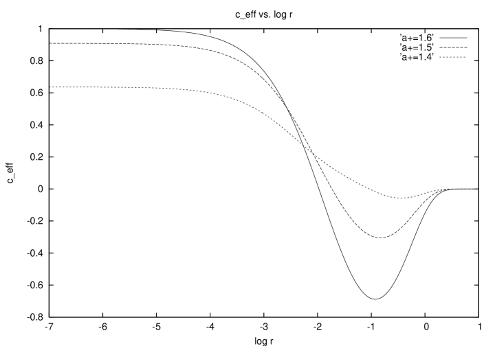
Figure 2: $c_{eff}$ vs. $\log r$, for $a_{+}=a_{-}=1.4\,,1.5\,,1.6$, with $\nu=2.2$ and $b_{+}=-b_{-}=1.3$

Figure 3: $c_{eff}$ vs. $a_{+}=a_{-}$, for $r=10^{-5}\,,0.1\,,0.3\,,1.0\,,10$, with $\nu=1.7$ and $b_{+}=b_{-}=0$

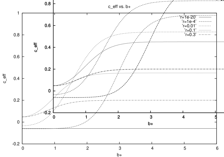
Figure 4: $c_{eff}$ vs. $b_{+}=-b_{-}$, for $r=10^{-20}\,,10^{-4}\,,0.01\,,0.1\,,0.3$, with $\nu=2.7$ and $a_{+}=a_{-}=1.4$

Figure 5: $c_{eff}$ vs. $\log r$, for $\nu=1.9\,,2.0\,,2.1$, with $a_{+}=1.7\,,a_{-}=1.5\,,b_{+}=-b_{-}=0.5$

References

- [1] M. Gaudin, Phys. Rev. A4 (1971) 386; La fonction d’onde de Bethe (Masson, 1983).
- [2] F.C. Alcaraz, M.N. Barber, M.T. Batchelor, R.J. Baxter and G.R.W. Quispel, J. Phys. A20 (1987) 6397.
- [3] C.J. Hamer, G.R.W. Quispel and M.T. Batchelor, J. Phys. A20 (1987) 5677.
- [4] E.K. Sklyanin, J. Phys. A21 (1988) 2375.
- [5] H.J. de Vega and A. González-Ruiz, J. Phys. A26 (1993) L519.
- [6] S. Ghoshal and A.B. Zamolodchikov, Int. J. Mod. Phys. A9 (1994) 3841.
- [7] P. Fendley and H. Saleur, Nucl. Phys. B428 (1994) 681.
- [8] M. Grisaru, L. Mezincescu and R.I. Nepomechie, J. Phys. A28 (1995) 1027.
- [9] A. LeClair, G. Mussardo, H. Saleur and S. Skorik, Nucl. Phys. B453 (1995) 581.
- [10] A. Doikou and R.I. Nepomechie, J. Phys. A32 (1999) 3663.
- [11] Al. Zamolodchikov, invited talk at the 4th Bologna Workshop, June 1999.
- [12] Z. Bajnok, L. Palla and G. Takacs, Nucl. Phys. B622 (2002) 565.
- [13] J.-S. Caux, H. Saleur and F. Siano, Phys. Rev. Lett. 88 (2002) 106402.
- [14] T. Lee and C. Rim, “Thermodynamic Bethe Ansatz for boundary sine-Gordon model,” hep-th/0301075
- [15] J.-S. Caux, H. Saleur and F. Siano, “The two-boundary sine-Gordon model,” cond-mat/0306328
- [16] R.I. Nepomechie, J. Stat. Phys. 111 (2003) 1363.
- [17] J. Cao, H.-Q. Lin, K.-J. Shi, Y. Wang, “Exact solutions and elementary excitations in the XXZ spin chain with unparallel boundary fields,” cond-mat/0212163
- [18] R.I. Nepomechie, “Bethe Ansatz solution of the open XXZ chain with nondiagonal boundary terms,” hep-th/0304092
- [19] R.I. Nepomechie and F. Ravanini, “Completeness of the Bethe Ansatz solution of the open XXZ chain with nondiagonal boundary terms,” hep-th/0307095
- [20] C. Destri and H.J. de Vega, Nucl. Phys. B290 (1987) 363.
- [21] H.J. de Vega, Int. J. Mod. Phys. A4 (1989) 2371.
- [22] N.Yu. Reshetikhin and H. Saleur, Nucl. Phys. B419 (1994) 507.
- [23] P.A. Pearce and A. Klümper, Phys. Rev. Lett. 68 (1991) 974; A. Klümper and P.A. Pearce, J. Stat. Phys. 64 (1991) 13.
- [24] C. Destri and H.J. de Vega, Phys. Rev. Lett. 69 (1992) 2313; Nucl. Phys. B504 (1997) 621.
- [25] D. Fioravanti, A. Mariottini, E. Quattrini and F. Ravanini, Phys. Lett. B390 (1997) 243.
- [26] H.W.J. Blöte, J.L. Cardy and M.P. Nightingale, Phys. Rev. Lett. 56 (1986) 742.
- [27] I. Affleck, Phys. Rev. Lett. 56 (1986) 746.
- [28] C.N. Yang and C.P. Yang, Phys. Rev. 150 (1966) 327.
- [29] E.T. Whittaker and G.N. Watson, A Course of Modern Analysis (Cambridge University Press, 1988).
- [30] F. Woynarovich and H.-P. Eckle, J. Phys. A20 (1987) L97.
- [31] M. Bauer and H. Saleur, Nucl. Phys. B320 (1989) 591.
- [32] Al. Zamolodchikov, Int. J. Mod. Phys. A10 (1995) 1125.
- [33] M. Ameduri, R. Konik and A. LeClair, Phys. Lett. B354 (1995) 376.
- [34] F. Ravanini, private communication.
- [35] C. Ahn, M. Bellacosa and F. Ravanini, “Finite size excited states for sine-Gordon model with Dirichlet boundary conditions,” in preparation.