Kinks in Discrete Light Cone Quantization

Abstract

We investigate non-trivial topological structures in Discrete Light Cone Quantization (DLCQ) through the example of the broken symmetry phase of the two dimensional $\phi^{4}$ theory using anti periodic boundary condition (APBC). We present evidence for degenerate ground states which is both a signature of spontaneous symmetry breaking and mandatory for the existence of kinks. Guided by a constrained variational calculation with a coherent state ansatz, we then extract the vacuum energy and kink mass and compare with classical and semi - classical results. We compare the DLCQ results for the number density of bosons in the kink state and the Fourier transform of the form factor of the kink with corresponding observables in the coherent variational kink state.

1. Introduction

Motivated by the remarkable work of Rozowsky and Thorn RT , we have recently investigated pp1 the broken symmetry phase of two dimensional $\phi^{4}$ theory in DLCQ dlcq with periodic boundary condition (PBC) without the zero momentum mode. Using a coherent state variational calculation as a guide, we extracted the vacuum energy density and kink mass from the results of matrix diagonalization. We also presented the Fourier transform of the form factor of the lowest excitation as well as the number density of elementary constituents of that state. Since the zero momentum mode was dropped in these investigations RT ; pp1 , the lowest state appeared as a kink-antikink pair because of the periodic boundary condition which implies that we are working in the sector with topological charge equal to zero. The results from these studies are not free from ambiguity at least in the finite volume because of the potential role played by the constrained zero momentum mode. With anti periodic boundary condition (APBC), the zero momentum mode is absent and hence calculations are free from the ambiguity created when it is simply neglected. With APBC one expects the ground state to be a kink or an antikink.

The quantum kink on the light front was addressed first by Baacke Baacke in the context of semi-classical quantization. As Baacke indicated, light front quantization offers the advantage of preserving translational invariance. To extract the kink mass in the classical theory he approximately diagonalized the mass operator ($M^{2}=P^{+}P^{-}$). He pointed out the advantage of light front quantization in handling the translation mode.

In this work we address the problem of the Fock space description of the topological structure in quantum field theory in the context of kinks that appear in the broken symmetry phase of two dimensional $\phi^{4}$ theory. As further background, it is worthwhile to recall that the study of these objects in lattice field theory is also highly non-trivial Ciria ; Ardekani . Within our own approach, we must qualify results by uncertainty due to unknown artifacts arising from discretization.

2. Notation and Conventions

We start from the Lagrangian density

$${\cal L}=\frac{1}{2}\partial^{\mu}\phi\partial_{\mu}\phi+\frac{1}{2}\mu^{2}\phi^{2}-\frac{\lambda}{4!}\phi^{4}.$$ (1)

The light front variables are defined by $x^{\pm}=x^{0}\pm x^{1}$.

The Hamiltonian density

$${\cal P}^{-}=-\frac{1}{2}\mu^{2}\phi^{2}+\frac{\lambda}{4!}\phi^{4}$$ (2)

defines the Hamiltonian

$$P^{-} = \int dx^{-}{\cal P}^{-}~{}\equiv\frac{L}{2\pi}H$$ (3)

where $L$ defines our compact domain $-L\leq x^{-}\leq+L$. Throughout this work we address the energy spectrum of $H$.

The longitudinal momentum operator is

$$P^{+} = \frac{1}{2}\int_{-L}^{+L}dx^{-}\partial^{+}\phi\partial^{+}\phi\equiv\frac{2\pi}{L}K$$ (4)

where $K$ is the dimensionless longitudinal momentum operator. The mass squared operator $M^{2}=P^{+}P^{-}=KH$.

In DLCQ with APBC, the field expansion has the form

$$\Phi(x^{-})=\frac{1}{\sqrt{4\pi}}\sum_{n}\frac{1}{\sqrt{n}}\left[a_{n}e^{-i\frac{n\pi}{L}x^{-}}+a_{n}^{\dagger}e^{i\frac{n\pi}{L}x^{-}}\right].$$ (5)

Here $n=\frac{1}{2},\frac{3}{2},\ldots.$

The normal ordered Hamiltonian is given by

$$H = -\mu^{2}\sum_{n}\frac{1}{n}a_{n}^{\dagger}a_{n}+\frac{\lambda}{4\pi}\sum_{k\leq l,m\leq n}~{}\frac{1}{N_{kl}^{2}}\frac{1}{\sqrt{klmn}}a_{k}^{\dagger}a_{l}^{\dagger}a_{n}a_{m}\delta_{k+l,m+n}$$ (6)

$$+\frac{\lambda}{4\pi}\sum_{k,l\leq m\leq n}~{}\frac{1}{N_{lmn}^{2}}\left[a_{k}^{\dagger}a_{l}a_{m}a_{n}+a_{n}^{\dagger}a_{m}^{\dagger}a_{l}^{\dagger}a_{k}\right]~{}\delta_{k,l+m+n}$$

with

$$N_{lmn} = 1,~{}l\neq m\neq n,$$ (7)

$$= \sqrt{2!},~{}l=m\neq n,~{}l\neq m=n,$$

$$= \sqrt{3!},~{}l=m=n,$$

and

$$N_{kl} = 1,k\neq l,~{}$$ (8)

$$= \sqrt{2!},~{}k=l.$$

3. Coherent State Calculations

Rozowsky and Thorn RT carried out a coherent state variational calculation for DLCQ in the case of PBC without the zero momentum mode. In this section we carry out the analogous calculation for APBC. The result of this calculation, being semi-classical, is especially reliable in the weak coupling region and we can use its functional form to extract the kink mass from the numerical results of matrix diagonalization.

Choose as a trial state, the coherent state

$$\mid\alpha\rangle={\cal N}e^{\sum_{n}\alpha_{n}a_{n}^{\dagger}}\mid 0\rangle$$ (9)

where ${\cal N}$ is a normalization factor.

With APBC we have

$$\frac{\langle\alpha\mid\phi(x^{-})\mid\alpha\rangle}{\langle\alpha\mid\alpha\rangle}=\frac{1}{\sqrt{4\pi}}~{}f(x^{-})$$ (10)

with

$$f(x^{-})=\sum_{m=1}^{N}\frac{1}{\sqrt{m-\frac{1}{2}}}\Big{[}\alpha_{m-\frac{1}{2}}e^{-i\frac{\pi}{L}(m-\frac{1}{2})x^{-}}+\alpha_{m-\frac{1}{2}}^{*}e^{i\frac{\pi}{L}(m-\frac{1}{2})x^{-}}\Big{]}~{}.$$ (11)

Minimizing the expectation value of the Hamiltonian, we obtain

$$f_{min}=\pm\sqrt{\frac{24\pi\mu^{2}}{\lambda}}=\pm\sqrt{\frac{3}{g}}.$$ (12)

Set

$$f(x^{-}) = \sqrt{\frac{3}{g}},~{}~{}0<x^{-}<L~{},$$ (13)

$$= -\sqrt{\frac{3}{g}},~{}~{}-L<x^{-}<0~{}.$$

Then we get

$$\alpha_{m-\frac{1}{2}}=\sqrt{\frac{3}{g}}~{}\frac{i}{\pi}~{}\frac{1}{\sqrt{m-\frac{1}{2}}}~{},~{}~{}m=1,2,3,\ldots,$$ (14)

and

$$f(x^{-})=\frac{2}{\pi}\sqrt{\frac{3}{g}}\sum_{j}\frac{1}{j}~{}\sin~{}\frac{j\pi x^{-}}{L}~{}$$ (15)

where $j=\frac{1}{2},\frac{3}{2},\frac{5}{2},$ etc. The number density of bosons with momentum fraction $x(=\frac{j}{K})$ is given by

$$\chi(x) = \frac{\langle\alpha\mid a_{j}^{\dagger}a_{j}\mid\alpha\rangle}{\langle\alpha\mid\alpha\rangle}=\alpha_{j}^{2}$$ (16)

where $\alpha_{j}\sim\frac{1}{\sqrt{j}}$.

In this case we get

$$\frac{1}{\langle\alpha\mid\alpha\rangle}\frac{2\pi}{L}\int dx^{-}\langle\alpha\mid\phi^{2}(x^{-})\mid\alpha\rangle=\frac{8}{\pi^{2}}\frac{3}{g}\sum_{j}\frac{1}{j^{2}}$$ (17)

where $j=1,3,5,\ldots.$ In the unconstrained variational calculation for PBC, the expectation value of the longitudinal momentum operator is infinite since $f(x^{-})$ is discontinous at $x^{-}=0$. To cure this deficiency, Rozowsky and Thorn performed a constrained variational calculation. Here we provide an outline of the analogous calculation for APBC. For constrained variational calculation in the case of PBC with the inclusion of a zero mode, see Ref. sugi .

With $\langle K\rangle=\frac{L}{2\pi}\frac{\langle\alpha\mid P^{+}\mid\alpha\rangle}{\langle\alpha\mid\alpha\rangle}$, and $f^{\prime}=\frac{\partial f(x^{-})}{\partial x^{-}}$ we have

$$K=\frac{L}{4\pi^{2}}\int_{-L}^{+L}dx^{-}(f^{\prime})^{2}~{}.$$ (18)

Minimizing

$$\frac{1}{\mu^{2}}~{}\frac{\langle\alpha\mid H_{\beta}\mid\alpha\rangle}{\langle\alpha\mid\alpha\rangle}=\frac{1}{L}\int_{-L}^{+L}dx^{-}\Big{[}\beta\Big{\{}\frac{L^{2}}{4\pi^{2}}(f^{\prime})^{2}-\langle K\rangle L\Big{\}}-\frac{1}{4}f^{2}+\frac{\lambda}{192\mu^{2}}f^{4}\Big{]}$$ (19)

we obtain

$$-2\beta\frac{L^{2}}{4\pi^{2}}\frac{\partial^{2}f}{\partial(x^{-})^{2}}-\frac{1}{2}f+\frac{\lambda}{48\pi\mu^{2}}f^{3}=0.$$ (20)

Putting $f(x^{-})=f_{0}F(u)$ where the variable $u=\frac{2x^{-}+L}{L}{\overline{K}}$ with

$${\overline{K}}={\overline{K}}(k)=\int_{0}^{1}dt(1-t^{2})^{-\frac{1}{2}}(1-k^{2}t^{2})^{-\frac{1}{2}},$$ (21)

we have,

$$\frac{\partial^{2}F}{\partial u^{2}}=-\frac{1}{4{\overline{K}}^{2}\beta}F+\frac{\lambda f_{0}^{2}}{96{\overline{K}}^{2}\beta\pi\mu^{2}}F^{3}.$$ (22)

Comparing with the differential equation satisfied by the Jacobi Elliptic Function $sn(u,k)$, namely,

$$\frac{\partial^{2}sn(u,k)}{\partial u^{2}}=-(1+k^{2})~{}sn(u,k)+2k^{2}~{}sn^{3}(u,k),$$ (23)

we get

$$f(x^{-})=f_{0}~{}sn\left(\frac{x^{-}}{L}{\overline{K}},k\right)$$ (24)

with

$$\beta=\frac{1}{4{\overline{K}}^{2}(1+k^{2})}~{}~{}{\rm and}~{}~{}f_{0}^{2}=\frac{48k^{2}\pi\mu^{2}}{\lambda(1+k^{2})}.$$ (25)

Note that we have imposed APBC on the solution. By explicit calculation we get

$$\langle K\rangle=\frac{8\mu^{2}}{\pi\lambda}{\overline{K}}\Big{[}E(k)-\frac{1-k^{2}}{1+k^{2}}{\overline{K}}(k)\Big{]}$$ (26)

with

$$E(k)=\int_{0}^{1}dt~{}\frac{\sqrt{1-k^{2}t^{2}}}{\sqrt{1-t^{2}}}$$ (27)

and

$$\frac{\langle\alpha\mid H\mid\alpha\rangle}{\langle\alpha\mid\alpha\rangle}=-\frac{24k^{2}\pi\mu^{4}}{\lambda(1+k^{2})^{2}}+\frac{64\mu^{6}}{\lambda^{2}(1+k^{2})\langle K\rangle}\Big{[}E(k)-\frac{1-k^{2}}{1+k^{2}}{\overline{K}}(k)\Big{]}^{2}.$$ (28)

In the $\langle K\rangle\rightarrow\infty$ limit, $k\rightarrow 1$ and we get

$$\frac{\langle\alpha\mid H\mid\alpha\rangle}{\langle\alpha\mid\alpha\rangle}=-\frac{6\pi\mu^{4}}{\lambda}+\frac{32\mu^{6}}{\lambda^{2}\langle K\rangle}~{}.$$ (29)

Interpreting the state $\mid\alpha\rangle$ to be a kink state, we identify the first term as the vacuum energy density which is the classical vacuum energy density. The second term is identified as $\frac{M_{kink}^{2}}{\langle K\rangle}$. Then we get the classical kink mass $M_{kink}=\frac{4\sqrt{2}\mu^{3}}{\lambda}$.

Using the Fourier expansion AS

$$sn(u,k)=\frac{1}{{\overline{K}}}\frac{2\pi}{\sqrt{k^{2}}}~{}\sum_{m=1}^{\infty}~{}\frac{q^{m-{1\over 2}}}{1-q^{2m-1}}~{}\sin\frac{(2m-1)\pi u}{2{\overline{K}}}$$ (30)

where $q=exp\left({-\pi\frac{{\overline{K}}(1-k^{2})}{{\overline{K}}(k^{2})}}\right)$ we have

$$f(x^{-})=\frac{2\pi}{{\overline{K}}}~{}\sqrt{\frac{48\pi\mu^{2}}{\lambda(1+k^{2})}}~{}\sum_{j}~{}\frac{q^{j}}{1-q^{2j}}~{}\sin\frac{j\pi x^{-}}{L}~{}.$$ (31)

In the limit $k^{2}\rightarrow 1$, using $q\rightarrow limit_{k^{2}\rightarrow 1}\left(1-\pi~{}\frac{{\overline{K}}(k^{2}-1)}{{\overline{K}}(k^{2})}\right)$ so that $(1-q^{2m-1}){\overline{K}}\rightarrow(2m-1)\frac{\pi^{2}}{2}$ since ${\overline{K}}(0)=\frac{\pi}{2}$, it is readily verified that in the limit $k^{2}\rightarrow 1$, the expression for $f(x^{-})$ in the constrained variational calculation given by Eq. (31) goes over to that in the unconstrained variational calculation given by Eq. (15).

4. Fourier transform of the form factor in DLCQ

An observable that yields considerable insight for the spatial structure of the topological object is the Fourier transform of its form factor. We compute the Fourier transform of the form factor of the lowest state which, according to Goldstone and Jackiw gj , in the weak coupling (static) limit, represents the kink profile. Let $\mid K\rangle$ and $\mid K^{\prime}\rangle$ denote this state with momenta $K$ and $K^{\prime}$. In the continuum theory,

$$\int_{-\infty}^{+\infty}dq^{+}exp\{-\frac{i}{2}q^{+}a\}\langle K^{\prime}\mid\Phi(x^{-})\mid K\rangle=\phi_{c}(x^{-}-a).$$ (32)

In DLCQ, we diagonalize the Hamiltonian for a given $K=\frac{L}{2\pi}P^{+}$. For the computation of the form factor, we need the same state at different $K$ values since $K^{\prime}=K+q$. We proceed as follows. We diagonalize the Hamiltonian, say, at $K=41$ (even particle sector). We diagonalize the Hamiltonian at the neighboring $K$ values, $K=40.5,41.5,39.5,42.5,38.5,43.5,37.5,44.5,36.5,45.5$ (odd particle sectors). In this particular example, the dimensionless momentum transfer ranges from $-4.5$ to $+4.5$. If $K$ is large enough to be near the continuum, then, in the spontaneous symmetry broken phase, with degenerate even and odd states, we can be confident that all these lowest states correspond to the same physical state observed at different longitudinal momenta. The test that the states are degenerate is that they have the same $M^{2}$, so the eigenvalues of $H$ fall on a linear trajectory as a function of $\frac{1}{K}$.

We proceed to compute the matrix element of the field operator between the lowest state at $K=40$ and the other specified values of $K$ and sum the amplitudes which corresponds to the choice of the shift parameter $a=0$. In summing the amplitudes, we need to be careful about the phases. First we note that $K$ is a conserved quantity, so eigenfunctions at different $K$ values have an independent arbitrary complex phase factor. To fix the phases, we accept the guidance of the coherent state analysis. We set the overall sign of the lowest states for all $K$ values such that the matrix elements $\langle K+n\mid a_{n}^{\dagger}\mid K\rangle~{}=~{}positive$ and $\langle K-n\mid a_{n}\mid K\rangle~{}=~{}negative$. In addition, there is one overall complex phase that we apply to the profile function so that it is real at the boundaries. That the sum of all terms for the profile function produces the shape of a kink, with very small imaginary component, is nevertheless a non-trivial result. It is a further non-trivial result that the magnitude of the kink represents a physically sensible result.

5. Numerical Results

With APBC, for integer (half integer) values of $K$ we have even (odd) number of particles. The dimensionality of the matrix in the even and odd sectors for different values of $K$ is presented in Table 1. All results presented here were obtained on small clusters of computers ($\leq$ 15 processors) using the Many Fermion Dynamics (MFD) code adapted to bosons mfd . The Lanczos diagonalization method is used in a highly scalable algorithm allowing us to proceed to sufficiently high values of K to numerically observe the phenomena we sought.

Since the Hamiltonian exhibits the $\phi\rightarrow-\phi$ symmetry, the even and odd particle sectors of the theory are decoupled. With a positive $\mu^{2}$, at weak coupling, the lowest state in the odd particle sector is a single particle carrying all the momentum. In the even particle sector, the lowest state consists of two particles. Thus for massive particles, there is a distinct mass gap between odd and even particle sectors. With a negative $\mu^{2}$, at weak coupling, the situation is drastically different. Now, the lowest states in the odd and even particle sectors consist of the maximum number of particles carrying the lowest allowed momentum. Thus, in the continuum limit, the possibility arises that the states in the even and odd particle sectors become degenerate. A clear signal of SSB is the degeneracy of the spectrum in the even and odd particle sectors. Thus at finite $K$, we can compare the spectra for an integer K value (even particle sector) and its neighboring half integer $K$ value (odd particle sector) and look for degenerate states. In Fig. 1 we show the lowest four energy eigenvalues in the broken symmetry phase for the even and odd particle sectors for $\lambda$=1.0 as a function of $\frac{1}{K}$. The points represent results at half integer increments in $K$ from $K=10$ to $K=55$. The overall trend is towards smoother behavior at higher $K$. There is an apparent small oscillation superimposed on a generally linear trend for each state. We believe that the oscillations represent an artifact of discretization. These oscillations decrease with increasing $K$. The smooth curves in Fig. 1 are linear fits to the eigenvalues in the range from $K=40$ to $K=55$ constrained to have the same intercept.

With guidance from the constrained variational calculation, see Eq. (29), we can extract the kink mass from the linear fit to the DLCQ data for the ground state eigenvalue. We fit the $\lambda=1.0$ data in the range $40\leq K\leq 55$ to a linear form ($C_{1}+C_{2}/K$). There are two reasons for this choice: (1) this is the maximum amount of data for which the $K$-artifacts seem reasonably absent; (2) independent fits and extrapolations from the four lowest eigenvalues are very close to each other at $K\rightarrow\infty$. We quote $C_{1}$ as the vacuum energy density and $C_{2}$ as the kink mass in Table 2. We obtain the uncertainties from the spread in these results arising from constrained fits to subsets of the data in this same range. For comparison, the corresponding classical values (classical vacuum energy density ${\cal E}=-6\pi\mu^{4}/\lambda$) are also presented. The agreement appears reasonable.

Next we examine the behavior of the number density $\chi(x)$ for the kink state. In the broken phase, the ground states in the even and odd particle sectors are degenerate in the continuum limit. In Fig. 2 we show $\chi(x)$ for $K=55$ and $K=54.5$ for $\lambda$ = 1. For this coupling the number densities for even and odd sectors are almost identical to each other indicative of degenerate states. In Fig. 2, we also compare the DLCQ number density with that predicted by the unconstrained and constrained variational calculations. At sufficiently large $K$ and low $\lambda$, they appear to agree at a level which is reasonable for the comparison of a quantal result with a semi-classical result.

Following Goldstone and Jackiw, we have calculated the Fourier transform of the form factor of the kink state in DLCQ at weak coupling. In Fig. 3(a) we show the profile calculated in DLCQ for $\lambda=1$ at three selected $K$ values. It is clear that at $\lambda=1$ the profile is that of a kink which appears reasonably converged with increasing $K$. In Fig. 3(b) we compare the $K=41$ DLCQ profile with that of a constrained variational coherent state calculation of Eq. (31) with $\langle K\rangle=41$. In the unconstrained variational calculation, this function is discontinuous at $x^{-}=0$ and $\langle K\rangle$, the expectation value of the dimensionless longitudinal momentum operator, is infinite. In the variational calculation where $\langle K\rangle$ is constrained to be finite, the kink profile is a smooth function of $x^{-}$ as seen in Fig. 3(b). In the limit $\langle K\rangle\rightarrow\infty$, the kink profile from constrained variational calculation approaches that of the unconstrained case. For each $K$ shown, we utilize 11 sets of DLCQ results to construct the profile function. Thus, for $K=41$ we employ results at $K=41$ and at $K=36.5$ through 45.5 in unit steps.

To summarize, we have demonstrated the existence of degenerate lowest eigenstates in two dimensional $\phi^{4}$ theory in DLCQ with APBC. The degeneracy of energy levels is both a signature of spontaneous symmetry breaking and essential for the existence of kinks. Using the constrained variational calculation as a guide, we have extracted the vacuum energy density and the kink mass for $\lambda=1$. We have extracted the number density of bosons in the kink state and compared it with predictions from coherent state variational calculations. We have also calculated the Fourier transform of the form factor of the kink and compared it with its counterpart in the variational approach. We interpret these results as indicative of the viability of DLCQ for addressing non-trivial phenomena in quantum field theory.

This work is supported in part by the Indo-US Collaboration project jointly funded by the U.S. National Science Foundation (INT0137066), the Department of Science and Technology, India (DST/INT/US (NSF-RP075)/2001). This work is also supported in part by the US Department of Energy, Grant No. DE-FG02-87ER40371, Division of Nuclear Physics and one of the authors (L.M.) was partially supported by the VEGA grant No.2/3106/2003. Two of the authors (D.C and A.H) acknowledge helpful discussions with Asit De and Samir Mallik.

=.1in =.1in =.1in

odd sector		even sector
K	dimension	K	dimension
15.5	295	16	336
31.5	12839	32	14219
39.5	61316	40	67243
44.5	151518	45	165498
49.5	358000	50	389253
54.5	813177	55	880962

Table 1: Dimensionality of the Hamiltonian matrix in odd and even particle sectors with anti periodic boundary condition.

=.1in =.1in =.1in

$\lambda$	vacuum energy		soliton mass
	classical	DLCQ	classical	semi-classical	DLCQ
1.0	-18.85	-18.73 $\pm 0.05$	5.66	5.19	5.3 $\pm 0.2$

Table 2: Comparison of vacuum energy density and soliton mass extracted from the continuum limit of our DLCQ data, with classical results. For soliton mass, the semi-classical result dashen is also shown.

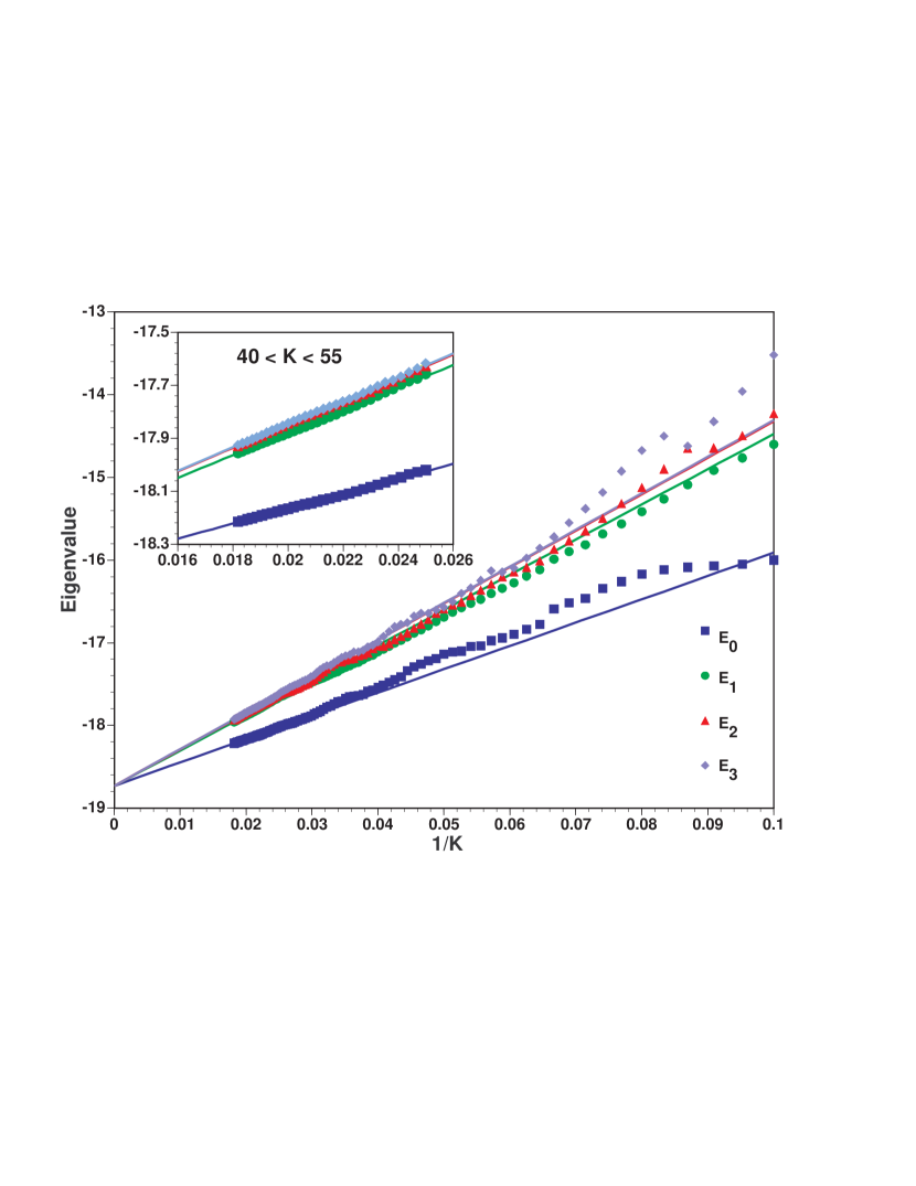
Figure 1: Lowest four eigenvalues for even and odd sectors as a function of $\frac{1}{K}$ for $\lambda$=1.0. The inset shows the details over the range $40\leq K\leq 55$. The discrete points are the DLCQ eigenvalues while the straight lines are the linear fits to the $40\leq K\leq 55$ data constrained to have the same intercept.

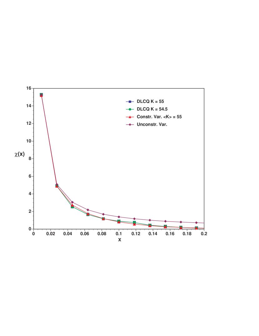
Figure 2: The number density $\chi(x)$ for even ($K=55.0$) and odd ($K=54.5$) sectors for $\lambda=1$ compared with unconstrained and constrained ($\langle K\rangle=55$) variational results.

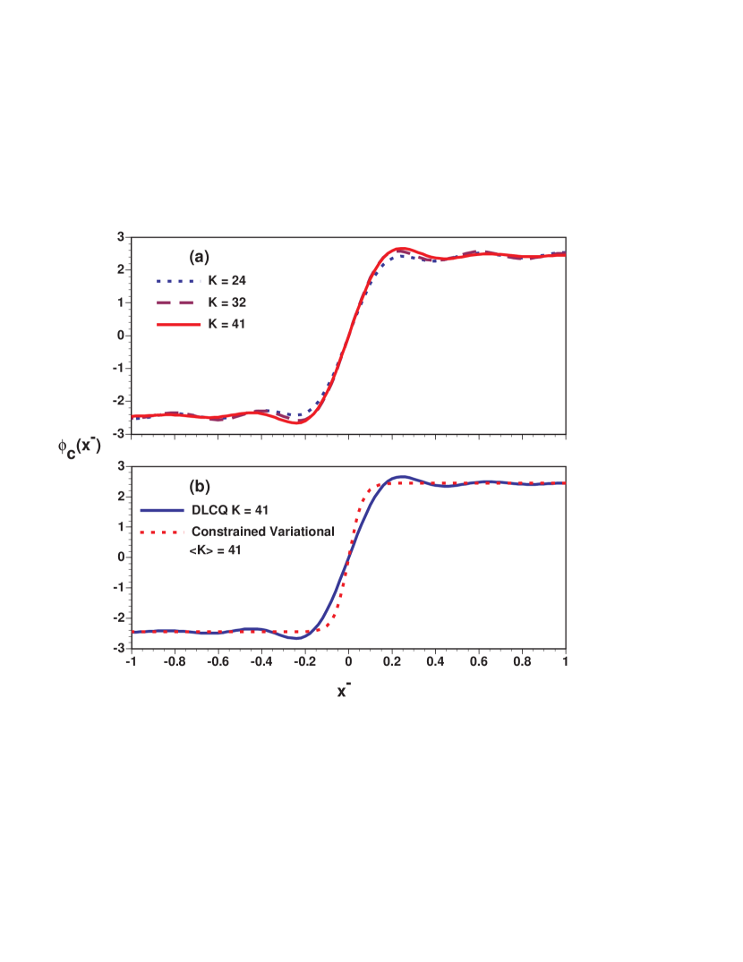
Figure 3: Fourier Transform of the kink form factor at $\lambda$=1; (a) results for $K=24,32$, and $41$ each obtained with DLCQ eigenstates from 11 values of $K$ centered on the designated $K$ value; (b) comparison of DLCQ profile at K=41 with constrained variational result with $\langle K\rangle=41$.

References

- (1) J. S. Rozowsky and C. B. Thorn, Phys. Rev. Lett. 85, 1614 (2000) [arXiv:hep-th/0003301].
- (2) Dipankar Chakrabarti, A. Harindranath, L. Martinovic, G. Pivovarov and J.P. Vary, manuscript in preparation.
- (3) T. Maskawa and K. Yamawaki, Prog. Theor. Phys. 56, 270 (1976); A. Casher, Phys. Rev. D14, 452 (1976); C. B. Thorn, Phys. Rev. D17, 1073 (1978); H.C. Pauli and S.J. Brodsky, Phys. Rev. D32, 1993, (1985); ibid., 2001 (1985).
- (4) J. Baacke, Z. Phys. C 1, 349 (1979).
- (5) J. C. Ciria and A. Tarancon, Phys. Rev. D 49, 1020 (1994) [arXiv:hep-lat/9309019].
- (6) A. Ardekani and A. G. Williams, Austral. J. Phys. 52, 929 (1999) [arXiv:hep-lat/9811002].
- (7) T. Sugihara and M. Taniguchi, Phys. Rev. Lett. 87, 271601 (2001) [arXiv:hep-th/0104012].
- (8) M. Abramovitz and I. Stegun, Handbook of Mathematical Functions with Formulas, Graphs, and Mathematical Tables, (Dover Publications, Inc., New York, 1972)
- (9) J. Goldstone and R. Jackiw, Phys. Rev. D 11, 1486 (1975).
- (10) J.P. Vary, The Many-Fermion-Dynamics Shell-Model Code, Iowa State University, 1992 (unpublished); J.P. Vary and D.C. Zheng, ibid., 1994.
- (11) R. F. Dashen, B. Hasslacher and A. Neveu, Phys. Rev. D 10, 4130 (1974).
=.1in \arraylinesep=.1in \extrarulesep=.1in