ITP-UU-03/49

SPIN-03/30

Cosmological backgrounds of superstring theory and Solvable Algebras: Oxidation and Branes^†
P. Fré¹, V. Gili², F. Gargiulo¹,
A. Sorin³, K. Rulik¹, M. Trigiante⁴

¹ Dipartimento di Fisica Teorica, Universitá di Torino, $\&$ INFN - Sezione di Torino

via P. Giuria 1, I-10125 Torino, Italy

² Dipartimento di Fisica Nucleare e Teorica, Universitá di Pavia, $\&$ INFN Sezione di Pavia

via A. Bassi 6, I-27100 Pavia, Italy

³ Bogoliubov Laboratory of Theoretical Physics, JINR, 141980 Dubna, Moscow Region, Russian Federation

⁴ Spinoza Institute, Leuvenlaan 4, Utrecht, The Netherlands

We develop a systematic algorithm to construct, classify and study exact solutions of type II A/B supergravity which are time–dependent and homogeneous and hence represent candidate cosmological backgrounds. Using the formalism of solvable Lie algebras to represent the geometry of non–compact coset manifolds $\mathrm{U/H}$ we are able to reduce the supergravity field equations to the geodesic equations in $\mathrm{U/H}$ and rephrase these latter in a completely algebraic setup by means of the so called Nomizu operator representation of covariant derivatives in solvable group manifolds. In this way a systematic method of integration of supergravity equations is provided. We show how the possible $D=3$ solutions are classified by non–compact subalgebras $\mathbf{G}\subset\mathrm{E_{8(8)}}$ and their ten–dimensional physical interpretation (oxidation) depends on the classification of the different embeddings $\mathbf{G}\hookrightarrow\mathrm{E_{8(8)}}$. We give some preliminary examples of explicit solutions based on the simplest choice $\mathbf{G}=\mathrm{A_{2}}$. We also show how, upon oxidation, these solutions provide a smooth and exact realization of the bouncing phenomenon on Weyl chamber walls envisaged by the cosmological billiards of Damour et al. We also show how this physical phenomenon is triggered by the presence of euclidean $D$–branes possibly interpretable at the microscopic level as S–branes. We outline how our analysis could be extended to a wider setup where, by further reducing to $D=2,1$, more general backgrounds could be constructed applying our method to the infinite algebras $E_{9,10}$.

 ^† This work is supported in part by the European Union RTN contracts HPRN-CT-2000-00122 and HPRN-CT-2000-00131. The work of M. T. is supported by an European Community Marie Curie Fellowship under contract HPMF-CT-2001-01276.

1 Introduction

In view of the new observational data in cosmology that appear to confirm the inflationary scenario and provide evidence for a small but positive cosmological constant [1, 2], there has been wide interest in the context of M–theory/string theory and extended supergravities for the search of de Sitter like vacua (see for instance [3]–[6] and references therein) and more generally for the analysis of time–dependent backgrounds [7]–[16]. This has been done in various approaches and at different levels, namely both from the microscopic viewpoint, considering time–dependent boundary states and boundary CFTs (see for instance [17, 18] and references therein) and from the macroscopic viewpoint studying supergravity solutions. In this latter context, great attention has been devoted to the classification of gaugings [19, 41, 42, 43, 44] their relation to compactifications with fluxes [20] and the ensuing cosmological solutions [3, 4, 5]. Indeed de Sitter like or anti de Sitter like backgrounds require an effective cosmological constant, or better a scalar potential that is typically produced by the gauging procedure.

As it is well known, gauged supergravities apparently break the large symmetry groups of ungauged supergravities encoding those perturbative and non perturbative dualities which are responsible for knitting together the five consistent perturbative superstrings into a single non–perturbative theory. Yet the interpretation of gaugings as compactifications with suitable fluxes and branes restores the apparently lost symmetries.

Notwithstanding this fact it is, to begin with, very much interesting to study cosmological backgrounds of superstring theory in the context of pure ungauged supergravity where the role of duality symmetries is more direct and evident.

In this setup a very much appealing and intriguing scenario has been proposed in a series of papers [21]–[31]: that of cosmological billiards. Studying the asymptotic behaviour of supergravity field equations near time (space–like) singularities, these authors have envisaged the possibility that the nine cosmological scale factors relative to the different space dimensions of string theory plus the dilaton could be assimilated to the lagrangian coordinates of a fictitious ball moving in a ten–dimensional space. This space is actually the Weyl chamber associated with the $E_{10}$ Dynkin diagram and the cosmological ball scatters on the Weyl chamber walls in a chaotic motion.

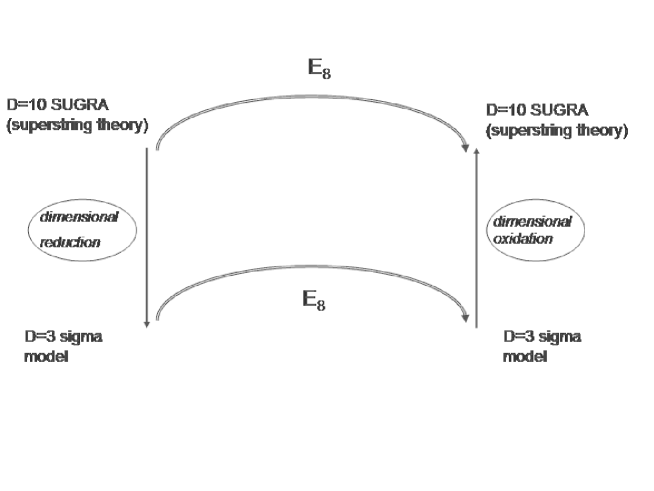
Figure 1: Time–dependent homogeneous supergravity backgrounds in $D=10$ can be obtained by first dimensionally reducing to $D=3$, solving the differential equations of the sigma model and then oxiding back the result to $D=10$. This procedure defines also the action of the hidden symmetry group $E_{8(8)}$ on the ten dimensional configurations.

There is a clear relation between this picture and the duality groups of superstring theories. Indeed it is well known that compactifying type II A or type II B supergravity on a $T^{r-1}$ torus, the massless scalars which emerge from the Kaluza-Klein mechanism in dimension $D=10-r+1$ just parametrize the maximally non–compact coset manifold

$$\mathcal{M}_{scalar}\,=\,\frac{\mathrm{E_{r(r)}}}{\mathrm{H_{r}}}$$ (1.1)

where $H_{r}$ is the maximally compact subgroup of the simple Lie group $\mathrm{E_{r(r)}}$ [32]. Furthermore the restriction of $\mathrm{E_{r(r)}}$ to integers is believed to be an exact non–perturbative symmetry of superstring theory compactified on such a torus [33]. Since compactification and truncation to the massless modes is an alternative way of saying that we just focus on field configurations that depend only the remaining:

$$10-r+1\,\mbox{coordinates}$$

it follows that cosmological backgrounds, where the only non trivial dependence is just on one coordinate, namely time, should be related to compactifications on a $T^{9}$ torus and hence linked to the $E_{10}$ algebra [34]–[38]. Furthermore the Cartan generators of the $\mathrm{E_{r(r)}}$ algebra are dual to the radii of the $T^{r-1}$ torus plus the dilaton. So it is no surprise that the evolution of the cosmological scale factor should indeed represent some kind of motion in the dual of the Cartan subalgebra of $E_{10}$. Although naturally motivated, the $E_{10}$ billiard picture was so far considered only in the framework of an approximated asymptotic analysis and no exact solution with such a behaviour was actually constructed. This originates from two main difficulties. Firstly, while up to $r=8$, which corresponds $D=3$ dimensions, the Lie algebras $E_{r(r)}$ are normal finite dimensional simple algebras, for $r=9,10$ they become infinite dimensional algebras whose structure is much more difficult to deal with and the corresponding coset manifolds need new insight in order to be defined. Secondly, the very billiard phenomenon, namely the scattering of the fictitious ball on the Weyl chamber walls requires the presence of such potential walls. Physically they are created by the other bosonic fields present in the supergravity theory, namely the non diagonal coefficients of the metric and the various $p$–form field strengths.

In this paper we focus on three–dimensional maximal supergravity [39]–[43], namely on the dimensional reduction of type II theories on a $\mathrm{T^{7}}$ torus, instead of going all the way down to reduction to one–dimension, by compactifying on $\mathrm{T^{9}}$. The advantage of this choice is that all the bosonic fields are already scalar fields, described by a non–linear sigma model without, however, the need of considering Kač–Moody algebras which arise as isometry algebras of scalar manifolds in $D<3$ space–times. In this way we are able to utilize the solvable Lie algebra approach to the description of the whole bosonic sector which enables us to give a completely algebraic characterization of the microscopic origin of the various degrees of freedom [45, 46]. Within this framework the supergravity field equations for bosonic fields restricted to only time dependence reduce simply to the geodesic equations in the target manifold $\mathrm{E_{8(8)}/SO(16)}$. These latter can be further simplified to a set of differential equations whose structure is completely determined in Lie algebra terms. This is done through the use of the so called Nomizu operator. The concept of Nomizu operator coincides with the concept of covariant derivative for solvable group manifolds and the possibility of writing covariant derivatives in this algebraic way as linear operators on solvable algebras relies on the theorem that states that a non–compact coset manifold with a transitive solvable group of isometries is isometrical to the solvable group itself.

The underlying idea for our approach is rooted in the concept of hidden symmetries. Cosmological backgrounds of superstring theory, being effectively one–dimensional fill orbits under the action of a very large symmetry group, possibly $\mathrm{E_{10}}$ that necessarily contains $\mathrm{E_{8(8)}}$, as the manifest subgroup in three dimensions. Neither $\mathrm{E_{10}}$ nor $\mathrm{E_{8(8)}}$ are manifest in $10$–dimensions but become manifest in lower dimension. So an efficient approach to finding spatially homogeneous solutions in ten dimensions consists of the process schematically described in fig.1. First one reduces to $D=3$, then solves the geodesic equations in the algebraic setup provided by the Nomizu–operator–formalism and then oxides back the result to a full fledged $D=10$ configuration. Each possible $D=3$ solution is characterized by a non–compact subalgebra

$$\mathbf{G}\,\subset\,\mathrm{{E}_{8(8)}}$$ (1.2)

which defines the smallest consistent truncation of the full supergravity theory within which the considered solution can be described. The inverse process of oxidation is not unique but leads to as many physically different ten dimensional solutions as there are algebraically inequivalent ways of embedding $\mathbf{G}$ into $\mathrm{E_{8(8)}}$. In this paper we will illustrate this procedure by choosing for $\mathbf{G}$ the smallest non abelian rank two algebra, namely $\mathbf{G}=\mathrm{A_{2}}$ and we will see that the non abelian structure of this algebra reflects interaction terms that are present in the ten dimensional theory like, for instance, the Chern–Simons term. The solvable Lie algebra formalism allows us to control, through the choice of the $\mathbf{G}$–embedding, the physical ten–dimensional interpretation of any given $\sigma$–model solution. In this paper we choose a particular embedding for the subalgebra $\mathrm{A_{2}}$ which leads to a type II B time dependent background generated by a system of two euclidean D-branes or S-branes [7, 8]: a D3 and a D1, whose world volumes are respectively four and two dimensional. This physical system contains also an essential non trivial B–field reflecting the three positive root structure of the $\mathrm{A_{2}}$ Lie algebra, one root being associated with the RR $2$–form $C^{[2]}$, a second with the RR $4$–form $C^{[4]}$ and the last with the NS $2$–form $B^{[2]}$. In the time evolution of this exact solution of type II B supergravity we retrieve a smooth realization of the bouncing phenomenon envisaged by the cosmic billiards of [21]–[31]. Indeed the scale factors corresponding to the dimensions parallel to the S–branes first expand and then, after reaching a maximum, contract. The reverse happens to the dimensions transverse to the $S$–branes. They display a minimum approximately at the same time when the parallel ones are maximal. Transformed to the dual CSA space this is the bouncing of the cosmic ball on a Weyl chamber wall. This is not yet the full cosmic billiard, but it illustrates the essential physical phenomena underlying its implementation. We shall argue that in order to obtain a repeated bouncing we need to consider larger subalgebras and in particular extend our analysis to the Kač–Moody case where the dual CSA becomes a space with lorentzian signature. Such an extension is postponed to future publications, yet we stress that the main features of the key ingredients for this analysis have been laid down here. Moreover it is worth emphasizing that the same $\mathrm{A_{2}}$ solution presented in this paper can be oxided to different ten–dimensional configurations corresponding to quite different physical systems. In particular, as we explain in later sections, it can be lifted to a purely gravitational background describing some sort of gravitational waves. In the present paper we give the general scheme, but the detailed study of these alternative oxidations is also postponed to future publications.

It is also worth mentioning that our approach to cosmological backgrounds makes it clear how, at least on the subspace of time dependent homogeneous configurations, the hidden symmetry $\mathrm{E_{8(8)}}$ or its further Kač–Moody extensions, can be made manifest directly in ten dimensions. Indeed it suffices to follow the diagram of fig.1. Reducing first to $D=3$, acting with the group and then oxiding back the result to ten dimensions defines the group action in ten dimensions.

Our paper is organized as follows. In section 2 after showing how three dimensional gravity can be decoupled from the sigma model, we recast the equations of motion of the latter into the geodesic equations for the manifold $\mathrm{E_{8(8)}/SO(16)}$ by using the Nomizu operator formalism. This leads to a system of first order non linear differential equations whose structure is completely encoded in the $\mathrm{E_{8(8)}}$ positive root system. In the same section we also outline an algorithm, valid for any maximally non compact homogeneous manifold $\mathrm{U/H}$, which allows to find the general solution of the geodesic differential system by means of compensating $\mathrm{H}$–transformations. Actually the original differential system is transformed into a new one for the parameters of the compensating $\mathrm{H}$–rotations which has the advantage of being integrable in an iterative way, namely by substituting at each step the solution of one differential equation into the next one.

In section 3 we apply the general method to an abstract $\mathrm{A_{2}}$–model, namely to the manifold $\mathrm{SL(3,\mathbb{R})/SO(3)}$. We derive explicit solutions of the differential equations which provide a paradigma to illustrate our method but also interesting examples which in a later section we oxide to ten dimensions.

In section 4 we construct the mathematical framework, based on the solvable Lie algebra formalism, which allows us to oxide any given solution of the three–dimensional theory to ten dimensions by choosing an embedding of the Lie algebra $\mathbf{G}$ into $\mathbf{E_{8(8)}}$.

In section 5 we consider the explicit oxidation of the $\mathrm{A_{2}}$ solutions previously found. First we classify the different available embeddings, which are of eight different types. Then, choosing the fourth type of embedding in our classification list, we show how it leads to a type II B supergravity solution which describes the already mentioned system of interacting $S3$ and $S1$ branes. We illustrate the physical properties of this solution also by plotting the time evolution of relevant physical quantities like the scale factors, the energy densities and the pressure eigenvalues. In this plots the reader can see the bouncing phenomenon described before.

Finally section 6 contains our conclusions and perspectives.

2 Geodesics on maximally non compact cosets $\mathrm{U}/\mathrm{H}$ and differential equations

We have recalled how both maximally extended supergravities (of type A and B) reduce, stepping down from $D=10$ to $D=3$ to the following non linear sigma model coupled to $D=3$ gravity:

$$\mathcal{L}^{\sigma-model}\,=\,\sqrt{-\mbox{det}\,g}\,\left[\,2\,R[g]\,+\,{\textstyle\frac{1}{2}}\,h_{IJ}\left(\phi\right)\partial_{\mu}\phi^{I}\partial_{\nu}\phi^{J}\,g^{\mu\nu}\right]$$ (2.1)

where $h_{IJ}$, $I,\,J\,=\,1,\,\ldots,\,128$, is the metric of the homogeneous $128$-dimensional coset manifold

$$\mathcal{M}_{128}=\frac{\mathrm{E_{8(8)}}}{\mathrm{SO(16)}}$$ (2.2)

The above manifold falls in the general category of manifolds $\mathrm{U/H}$ such that $\mathbb{U}$ (the Lie algebra of $\mathrm{U}$) is the maximally non-compact real section of a simple Lie algebra $\mathbb{U}_{C}$ and the subgroup $\mathrm{H}$ is generated by the maximal compact subalgebra $\mathbb{H}\subset\mathbb{U}$. In this case the solvable Lie algebra description of the target manifold $\mathrm{U/H}$ is universal. The manifold $\mathrm{U/H}$ is isometrical to the solvable group manifold:

$$\mathcal{M}_{d}=\exp\,\left[Solv\left(\mathrm{U/H}\right)\,\right]$$ (2.3)

where the solvable algebra $Solv\left(\mathrm{U/H}\right)$ is spanned by all the Cartan generators $\mathcal{H}_{i}$ and by the step operators $E^{\alpha}$ associated with all positive roots $\alpha>0$ (on the solvable Lie algebra parametrization of supergravity scalar manifolds see [45, 46]). On the other hand the maximal compact subalgebra $\mathbb{H}$ is spanned by all operators of the form $E_{\alpha}-E_{-\alpha}$ for all positive roots $\alpha>0$. So the dimension of the coset $d$, the rank $r$ of $\mathbb{U}$ and the number of positive roots $p$ are generally related as follows:

$$\mbox{dim}\left[U/H\right]\equiv d\,=\,r+p\quad;\quad p\,\equiv\,\#\mbox{positive roots}=\mbox{dim}\,\mathbb{H}\quad;\quad r\,\equiv\,\mbox{rank}\,\mathbb{U}$$ (2.4)

In the present section we concentrate on studying solutions of a bosonic field theory of type (2.1) that are only time-dependent. In so doing we consider the case of a generic manifold $\mathrm{U/H}$ and we show how the previously recalled algebraic structure allows to retrieve a complete generating solution of the field equations depending on as many essential parameters as the rank of the Lie algebra $\mathbb{U}$. These parameters label the orbits of solutions with respect to the action of the two symmetries present in (2.1), namely $\mathrm{U}$ global symmetry and $\mathrm{H}$ local symmetry.

The essential observation is that, as long as we are interested in solutions depending only on time, the field equations of (2.1) can be organized as follows. First we write the field equations of the matter fields $\phi^{I}$ which supposedly depend only on time. At this level the coupling of the sigma-model to three dimensional gravity can be disregarded. Indeed the effect of the metric $g_{00}$ is simply that the field equations for the scalars $\phi^{I}$ have the same form as they would have in a rigid sigma model with just the following proviso. The parameter we use is proper time rather than coordinate time. Next in the variation with respect to the metric we can use the essential feature of three–dimensional gravity, namely the fact that the Ricci tensor completely determines also the Riemann tensor. This means that from the stress energy tensor of the sigma model solution we reconstruct, via Einstein field equations, also the corresponding three dimensional metric.

2.1 Decoupling the sigma model from gravity

Since we are just interested in configurations where the fields depend only on time, we take the following ansatz for the three dimensional metric:

$$ds^{2}_{3D}=A^{2}(t)\,dt^{2}-B^{2}(t)\left(dr^{2}+r^{2}d\phi^{2}\right)$$ (2.5)

where $A(t)$ and $B(t)$ are undetermined functions of time. Then we observe that one of these functions can always be reabsorbed into a redefinition of the time variable. We fix such a coordinate gauge by requiring that the matter field equations for the sigma model should be decoupled from gravity, namely should have the same form as in a flat metric. This will occur for a special choice of the time variable. Let us see how.

In general, the sigma model equations, coupled to gravity, have the following form:

$$\Box_{cov}\,\phi^{I}+\Gamma^{I}_{JK}\partial_{\mu}\phi^{J}\,\partial_{\nu}\phi^{K}\,g^{\mu\nu}=0$$ (2.6)

In the case we restrict dependence only on time the above equations reduce to:

$$\frac{1}{\sqrt{-\mbox{det}g}}\,\frac{d}{dt}\left(\sqrt{-\mbox{det}g}\,g^{00}\,\frac{d}{dt}\,\phi^{I}\right)+\Gamma^{I}_{JK}\frac{d}{dt}\phi^{J}\,\frac{d}{dt}\phi^{K}\,g^{00}=0$$ (2.7)

We want to choose a new time $\tau=\tau(t)$ such that with respect to this new variable equations (2.7) take the same form as they would have in a sigma model in flat space, namely:

$$\ddot{\phi}^{I}\,+\,\Gamma^{I}_{JK}\,\dot{\phi}^{J}\,\dot{\phi}^{K}\,=\,0\qquad I,\,J,\,K\,=\,1,\,\ldots,\,\mbox{dim}\,\mathcal{M}$$ (2.8)

where $\Gamma^{I}_{JK}$ are the Christoffel symbols for the metric $h_{IJ}$. The last equations are immediately interpreted as geodesic equations in the target scalar manifold.

In order for equations (2.7) to reduce to (2.8) the following condition must be imposed:

$$\sqrt{-\mbox{det}g}\,g^{00}\,\frac{d}{dt}=\frac{d}{d\tau}\,\Rightarrow\,dt=\sqrt{-\mbox{det}g}\,g^{00}\,d\tau$$ (2.9)

Inserting the metric (2.5) into the above condition we obtain an equation for the coefficient $A(t)$ in terms of the coefficient $B(t)$. Indeed in the new coordinate $\tau$ the metric (2.5) becomes:

$$ds^{2}_{3D}=B^{4}(\tau)\,d\tau^{2}-B^{2}(\tau)\left(dr^{2}+r^{2}d\phi^{2}\right)$$ (2.10)

The choice (2.10) corresponds to the following choice of the dreibein:

$$e^{0}=B^{2}(\tau)\,d\tau\quad;\quad e^{1}=B(\tau)dr\quad;\quad e^{2}=B(\tau)\,r\,d\phi$$ (2.11)

For such a metric the curvature $2$-form is as follows:

$$R^{01} = \frac{2\dot{B}^{2}(\tau)-B(\tau)\,\ddot{B}(\tau)}{B^{6}(\tau)}\,e^{0}\,\wedge\,e^{1}$$

$$R^{02} = \frac{2\dot{B}^{2}(\tau)-B(\tau)\,\ddot{B}(\tau)}{B^{6}(\tau)}\,e^{0}\,\wedge\,e^{2}$$

$$R^{12} = -\frac{\dot{B}^{2}(\tau)}{B^{6}(\tau)}e^{1}\,\wedge\,e^{2}$$ (2.12)

The Einstein equations, following from our lagrangian (2.1) are the following ones, in flat indices:

$$2\,G_{ab}\,=\,T_{ab}\quad;\quad G_{ab}\equiv\mbox{Ric}_{ab}-{\textstyle\frac{1}{2}}\,R\,\eta_{ab}\quad;\quad a,b=0,1,2$$ (2.13)

With the above choice of the vielbein, the flat index Einstein tensor is easily calculated and has the following form:

$$G_{00}=\frac{\dot{B}^{2}(\tau)}{2\,B^{6}(\tau)}\quad;\quad G_{0i}=0\quad;\quad G_{ij}=\frac{2\,\dot{B}^{2}(\tau)-B(\tau)\,\ddot{B}(\tau)}{2\,B^{6}(\tau)}\,\delta_{ij}\quad;\quad i,j=1,2$$ (2.14)

On the other hand, calculating the stress energy tensor of the scalar matter in the background of the metric (2.10) we obtain (also in flat indices):

$$T_{00}=\frac{1}{2\,B^{4}(\tau)}\,\left(\dot{\phi}^{I}\dot{\phi}^{J}h_{IJ}\right)\quad;\quad T_{0i}=0\quad;\quad T_{ij}=\frac{1}{2\,B^{4}(\tau)}\,\left(\dot{\phi}^{I}\dot{\phi}^{J}h_{IJ}\right)\,\delta_{ij}\quad;\quad i,j=1,2$$ (2.15)

where

$$\dot{\phi}^{I}\dot{\phi}^{J}h_{IJ}=\varpi^{2}$$ (2.16)

is a constant independent from time as a consequence of the geodesic equations (2.8). To prove this it suffices to take a derivative in $\tau$ of ${\varpi^{2}}$ and verify that it is zero upon use of eq.s (2.8).

Hence in order to satisfy the coupled equations of gravity and matter fields it is necessary that:

$$2\,\frac{\dot{B}^{2}(\tau)}{2\,B^{6}(\tau)}=2\,\frac{2\,\dot{B}^{2}(\tau)-B(\tau)\,\ddot{B}(\tau)}{2\,B^{6}(\tau)}=\frac{1}{2\,B^{4}(\tau)}\,{\varpi^{2}}$$ (2.17)

The first of the above equalities implies:

$$\dot{B}=k\,B\quad\Rightarrow\quad B(\tau)=\exp[k\,\tau]$$ (2.18)

where $k$ is some constant. The second equality is satisfied if:

$$k=\pm{\textstyle\frac{1}{\sqrt{2}}}\,|\varpi|=\pm{\textstyle\frac{1}{\sqrt{2}}}\,\sqrt{\dot{\phi}^{I}\dot{\phi}^{J}h_{IJ}}$$ (2.19)

In this way we have completely fixed the metric of the three–dimensional space as determined by the solution of the geodesic equations for the scalar matter:

$$ds^{2}_{3D}=\exp\left[4k\,\tau\right]d\tau^{2}-\exp\left[2k\,\tau\right]\,\left(dx_{1}^{2}+dx_{2}^{2}\right)$$ (2.20)

with the parameter $k$ given by eq.(2.19).

2.2 Geodesic equations in target space and the Nomizu operator

Having clarified how the three dimensional metric is determined in terms of the solutions of the sigma model, we concentrate on this latter. We focus on the geodesic equations (2.8) and in order to study them, we rely on the solvable Lie group description of the target manifold going to an anholonomic basis for the tangent vectors to the geodesic. Since gravity is decoupled from the scalars, we deal with a rigid sigma-model where the fields depend only on time

$$\mathcal{L}^{\sigma-model}\propto h_{IJ}(\phi)\dot{\phi}^{I}\dot{\phi}^{J}$$ (2.21)

As was mentioned before, the equations of motion in this case reduce to the geodesic equations for the metric $h_{IJ}(\phi)$ and time plays the role of a parameter along the geodesics (see eq.(2.8)). Since $h_{IJ}(\phi)$ is the metric of a scalar manifold which is a maximally non-compact coset $\mathcal{M}=\mathrm{U/H}$, we can derive this metric from a coset representative $\mathbb{L}(\phi)\in U$

$$h_{IJ}(\phi)=\mathrm{Tr}(\mathbb{P}_{K}{\rm I\kern-1.79993ptL}^{-1}\partial_{I}{\rm I\kern-1.79993ptL}{\rm I\kern-1.79993ptL}^{-1}\partial_{J}{\rm I\kern-1.79993ptL})$$ (2.22)

$\mathbb{P}_{K}$ being a projection operator on the coset directions of the Lie algebra $\mathbb{U}$ to be discussed in a moment. To this effect we introduce the following general notation. We make the orthogonal split of the $\mathbb{U}$ Lie algebra:

$$\mathbb{U}=\mathbb{H}\oplus\mathbb{{K}}$$ (2.23)

where $\mathbb{H}\subset\mathbb{U}$ is the maximal compact subalgebra and $\mathbb{{K}}$ its orthogonal complement. We adopt the following normalizations for the generators in each subspace:

$$\mathbb{U}=\mathrm{Span}\{H_{i},E_{\alpha},E_{-\alpha}\}$$

$$\mathbb{K}=\mathrm{Span}\{K_{A}\}=\mathrm{Span}\{H_{i},{\textstyle\frac{1}{\sqrt{2}}}(E_{\alpha}+E_{-\alpha})\}$$ (2.24)

$$\mathbb{H}=\mathrm{Span}\{t_{\alpha}\}=\mathrm{Span}\{(E_{\alpha}-E_{-\alpha})\}$$

The ${\mathbb{U}}$ Lie-algebra valued left invariant one-form

$$\Omega=\mathbb{L}^{-1}d\mathbb{L}\,=\,V^{A}K_{A}+\omega^{\alpha}t_{\alpha}$$ (2.25)

is in general expanded along all the generators of $\mathbb{U}$ (not only along $\mathbb{{K}}$) and $V=V^{A}\,K_{A}$ corresponds to the coset manifold vielbein while $\omega=\omega^{\alpha}\,t_{\alpha}$ corresponds to the coset manifold $\mathrm{H}$–connection.

As it is well known neither the coset representative $\mathbb{L}(\phi)$, nor the one-form $\Omega$ are unique. Indeed $\mathbb{L}$ is defined up to multiplication on the right by an element of the compact subgroup $h\in H$. This is a gauge invariance which can be fixed in such a way that the coset representative lies in the solvable group ${Solv}(\mathrm{U/H})$ obtained by exponentiating the solvable subalgebra $Solv(\mathbb{U}/\mathbb{H})$

$$\mathbb{L}\left(\phi\right)\,=\,\exp{\left(Solv(\mathbb{U}/\mathbb{H})\cdot\phi\right)}$$ (2.26)

In the case of $\mathrm{U}/\mathrm{H}$ being maximally non compact $Solv(\mathbb{U}/\mathbb{H})$ coincides with the Borel subalgebra and therefore it is spanned by the collection of all Cartan generators and step-operators associated with positive roots, as we already stated, namely:

$$Solv(\mathbb{U}/\mathbb{H})=\mathrm{Span}\,\left\{T_{A}\right\}=\mathrm{Span}\,\left\{H_{i},E_{\alpha}\right\}$$ (2.27)

If the coset representative $\mathbb{L}$ is chosen to be a solvable group element, as in eq. (2.26), namely if we are in the solvable parametrization of the coset, we can also write:

$$\Omega=\mathbb{L}^{-1}d\mathbb{L}=\widetilde{V}^{i}\,\mathcal{H}_{i}\,+\,\widetilde{V}^{\alpha}\,E_{\alpha}=\widetilde{V}^{A}\,T_{A}$$ (2.28)

since $\Omega$ is contained in the solvable subalgebra $Solv(\mathbb{U}/\mathbb{H})\subset\mathbb{U}$. Eq.s (2.25) and (2.28) are compatible if and only if:

$$V^{\alpha}=\sqrt{2}\,\omega^{\alpha}$$ (2.29)

In this case we can identify $\widetilde{V}^{i}={V}^{i}$ and $\widetilde{V}^{\alpha}=\sqrt{2}\,V^{\alpha}$; eq.(2.29) is the solvability condition for a coset representative.

Hence we can just rewrite the metric of our maximally non–compact manifold $\mathrm{U}/\mathrm{H}$ as follows:

$$ds^{2}_{\mathrm{U}/\mathrm{H}}\,=\,\sum_{A=1}^{\mbox{dim}\mathrm{U}}V^{A}\,\otimes\,V^{A}=\widetilde{V}^{i}\oplus\widetilde{V}^{i}+{\textstyle\frac{1}{2}}\widetilde{V}^{\alpha}\oplus\widetilde{V}^{\alpha}$$ (2.30)

It is interesting to discuss what are the residual $\mathrm{H}$–gauge transformations that remain available after the solvable gauge condition (2.29) has been imposed. To this effect we consider the multiplication

$$\mathbb{L}\mapsto\mathbb{L}\,h=\overline{\mathbb{L}}$$ (2.31)

where

$$h=\exp\,\left[\theta^{\alpha}\,t_{\alpha}\right]$$ (2.32)

is a finite element of the $\mathrm{H}$ subgroup singled out by generic parameters theta. For any such element we can always write:

$$h^{-1}\,t_{\alpha}\,h = A(\theta)_{\alpha}^{\phantom{\alpha}\beta}\,t_{\beta}$$

$$h^{-1}\,K_{A}\,h = D(\theta)_{A}^{\phantom{A}B}\,K_{B}$$ (2.33)

where the matrix $A(\theta)$ is the adjoint representation of $h$ and $D(\theta)$ is the $D$–representation of the same group element. We obtain:

$$\overline{\Omega}\equiv\overline{\mathbb{L}}^{-1}\,d\overline{\mathbb{L}} = h^{-1}dh+h^{-1}\,\Omega\,h$$ (2.34)

$$= \underbrace{h^{-1}\,dh+h^{-1}\,\omega\,h}_{=\,\,\overline{\omega}}\,+\underbrace{\,h^{-1}\,V\,h}_{=\,\,\overline{V}}$$

where

$$\overline{\omega}^{\alpha} = \frac{1}{\mbox{tr}(t_{\alpha}^{2})}\,\mbox{tr}\left(h^{-1}\,dh\,t_{\alpha}\right)\,+\,\omega^{\beta}\,A(\theta)_{\beta}^{\phantom{\beta}\alpha}$$

$$\overline{V}^{\alpha} = V^{\beta}\,D(\theta)_{\beta}^{\phantom{\beta}\alpha}\,+\,V^{i}\,D(\theta)_{i}^{\phantom{i}\alpha}\,$$ (2.35)

Suppose now that the coset representative $\mathbb{L}$ is solvable, namely it satisfies eq.(2.29). The coset representative $\overline{\mathbb{L}}$ will still satisfy the same condition if the $h$-compensator satisfies the following condition:

$$\frac{\sqrt{2}}{\mbox{tr}(t_{\alpha}^{2})}\,\,\mbox{tr}\left(h^{-1}(\theta)\,dh(\theta)\,t_{\alpha}\right)=V^{\beta}\,\left(A(\theta)_{\beta}^{\phantom{\beta}\alpha}\,-\,D(\theta)_{\beta}^{\phantom{\beta}\alpha}\right)\,+\,V^{i}\,D(\theta)_{i}^{\phantom{i}\alpha}$$ (2.36)

The above equations are a set of $n=\#roots=\mbox{dim}H$ differential equations on the parameters $\theta^{\alpha}$ of the $h$–subgroup element (compensator). In the following we will use such set of equations as the basis of an algorithm to produce solutions of the geodesic equations (2.8).

Given these preliminaries, we can establish a new notation. We introduce tangent vectors to the geodesics in the anholonomic basis:

$$\Phi^{A}\,=\,\widetilde{V}^{A}_{I}\left(\phi\right)\dot{\phi}^{I}$$ (2.37)

which are functions only of time: $\Phi^{A}\,=\,\Phi^{A}(t)$. In this basis the field equations reduce to

$$\dot{\Phi}^{A}\,+\,\Gamma^{A}_{BC}\Phi^{B}\Phi^{C}\,=\,0$$ (2.38)

where now $\Gamma^{A}_{BC}$ are the components of the Levi-Civita connection in the chosen anholonomic basis. Explicitly they are related to the components of the Levi Civita connection in an arbitrary holonomic basis by:

$$\Gamma^{A}_{BC}\,=\Gamma^{I}_{JK}V^{A}_{I}V^{J}_{B}V^{K}_{C}-\partial_{K}(V^{A}_{J})V^{J}_{B}V^{K}_{C}$$ (2.39)

where the inverse vielbein is defined in the usual way:

$$V^{A}_{I}\,V^{I}_{B}\,=\,\delta^{A}_{B}$$ (2.40)

The most important point here is that, the connection $\Gamma^{A}_{BC}$ can be identified with the Nomizu connection defined on a solvable Lie algebra, if the coset representative $\mathbb{L}$ from which we construct the vielbein via eq.(2.25), is solvable, namely if and only if the solvability condition (2.29) is satisfied. In fact, as we can read in [47], once we have defined over $Solv$ a non degenerate, positive definite and symmetric form:

$$\langle\,,\,\rangle \;:\;Solv\otimes Solv\longrightarrow\mathbb{R}$$

$$\langle X\,,\,Y\rangle \;=\;\langle Y\,,\,X\rangle$$ (2.41)

whose lifting to the manifold produces the metric, the covariant derivative is defined through the Nomizu operator:

$$\forall X\in Solv\,:\,\mathbb{L}_{X}:Solv\longrightarrow Solv$$ (2.42)

so that

$$\forall X,Y,Z\in Solv\,:\,2\langle Z\,,\,\mathbb{L}_{X}Y\rangle\,=\,\langle Z,\left[X,Y\right]\rangle\,-\,\langle X,\left[Y,Z\right]\rangle\,-\,\langle Y,\left[X,Z\right]\rangle$$ (2.43)

while the Riemann curvature 2-form is given by the commutator of two Nomizu operators:

$$R^{W}_{\phantom{W}Z}\left(X,Y\right)\,=\,\langle W\,,\,\left\{\left[\mathbb{L}_{X},\mathbb{L}_{Y}\right]\,-\,\mathbb{L}_{\left[X,Y\right]}\right\}Z\rangle$$ (2.44)

This implies that the covariant derivative explicitly reads:

$$\mathbb{L}_{X}\,Y\,=\,\Gamma_{XY}^{Z}\,Z$$ (2.45)

where

$$\Gamma_{XY}^{Z}\,=\,{\textstyle\frac{1}{2}}\left(\langle Z,\left[X,Y\right]\rangle\,-\,\langle X,\left[Y,Z\right]\rangle\,-\,\langle Y,\left[X,Z\right]\rangle\right)\,\frac{1}{<Z,Z>}\,\qquad\,\forall X,Y,Z\in Solv$$ (2.46)

In concrete, the non degenerate, positive definite, symmetric form on the solvable Lie algebra which agrees with equation (2.30) is defined by setting:

$$\langle\mathcal{H}_{i}\,,\,\mathcal{H}_{j}\rangle \,=\, 2\,\delta_{ij}$$

$$\langle\mathcal{H}_{i}\,,\,E_{\alpha}\rangle \,=\, 0$$

$$\langle E_{\alpha}\,,\,E_{\beta}\rangle \,=\, \delta_{\alpha,\beta}$$ (2.47)

$\forall\mathcal{H}_{i},\,\mathcal{H}_{j}\,\in\,\mathrm{CSA}_{\mathrm{E_{8(8)}}}$ and $\forall E_{\alpha}$, step operator associated to a positive root $\alpha$ of $\mathrm{E_{8(8)}}$. Then the Nomizu connection (which is constant) is very easy to calculate. We have:

$$\begin{array}[]{lll}\Gamma^{i}_{jk}&\,=&\,0\\ \Gamma^{i}_{\alpha\beta}&\,=&\,{\textstyle\frac{1}{2}}\left(-\langle E_{\alpha},\,\left[E_{\beta},\,H^{i}\right]\rangle-\langle E_{\beta},\,\left[E_{\alpha},\,H^{i}\right]\rangle\right)\,=\,{\textstyle\frac{1}{2}}\,\alpha^{i}\delta_{\alpha\beta}\\ \Gamma^{\alpha}_{ij}&\,=&\,\Gamma^{\alpha}_{i\beta}\,=\,\Gamma^{i}_{j\alpha}\,=\,0\\ \Gamma^{\alpha}_{\beta i}&\,=&\,{\textstyle\frac{1}{2}}\left(\langle E^{\alpha},\,\left[E_{\beta},\,H_{i}\right]\rangle-\langle E_{\beta},\,\left[H_{i},\,E^{\alpha}\right]\rangle\right)\,=\,-\alpha_{i}\,\delta^{\alpha}_{\beta}\\ \Gamma^{\alpha+\beta}_{\alpha\beta}&\,=&\,-\Gamma^{\alpha+\beta}_{\beta\alpha}\,=\,{\textstyle\frac{1}{2}}N_{\alpha\beta}\\ \Gamma^{\alpha}_{\alpha+\beta\,\beta}&\,=&\,\Gamma^{\alpha}_{\beta\,\alpha+\beta}\,=\,{\textstyle\frac{1}{2}}N_{\alpha\beta}\end{array}$$

where $N_{\alpha\beta}$ is defined by the commutator:

$$\left[E_{\alpha}\,,\,E_{\beta}\right]\,=\,N_{\alpha\beta}\,E_{\alpha+\beta}$$ (2.48)

which has to be worked out in the algebra. Notice that $\Gamma^{Z}_{XY}\neq\Gamma^{Z}_{YX}$ since its expression consists of the first term which is antisymmetric in $(X,\,Y)$ and the sum of the last two which is symmetric. The component $\Gamma^{\alpha}_{\beta i}$ consists of the sum of two equal contributions from the antisymmetric and symmetric part, the same contributions cancel in $\Gamma^{\alpha}_{i\beta}$ which indeed vanishes. By substituting the explicit expression of the Nomizu connection in (2.38) and introducing for the further convenience new names for the tangent vectors along the Cartan generators $\chi^{i}\equiv\Phi^{i}$ we have the equations:

$$\dot{\chi}^{i} \,+\, \,{\textstyle\frac{1}{2}}\,\sum_{\alpha\in\Delta_{+}}\alpha^{i}\Phi_{\alpha}^{2}\,=\,0$$

$$\dot{\Phi}^{\alpha} \,+\, \,\sum_{\beta\in\Delta_{+}}\,N_{\alpha\beta}\Phi^{\beta}\Phi^{\alpha+\beta}-\alpha_{i}\,\chi^{i}\Phi^{\alpha}\,=\,0$$ (2.49)

Eq.s (2.2 ) encode all the algebraic structure of the $D=3$ sigma model and due to our oxidation algorithm of the original supergravity in ten dimensions.

All this means that, thanks to the solvability of the algebra (and also to the fact that we know the explicit form of the connection via the Nomizu operator), we have reduced the entire problem of finding time dependent backgrounds for either type II A or type II B superstrings or M-theory to the integration of a system of differential equations firmly based on the algebraic structure of $E_{8(8)}$. This is a system of non-linear differential equations, and from this point of view it might seem hopeless to be solved. Yet, due to its underlying algebraic structure, one can use its isometries to generate the complete integral depending on as many integration constants as the number of equations in the system. This is the compensator algorithm we alluded to above, which we shortly outline. To this effect we discuss the role of initial conditions for the tangent vectors to the geodesics. There exist a number of possibilities for such conditions that can truncate the whole system to smaller and simpler ones. The simplest choice is to put all root-vectors to zero in the origin. This will ensure that root-vectors will remain zero at all later times and the system will reduce to

$$\dot{\chi}^{i}=0$$ (2.50)

The solution of such a reduced system is trivial and consists of a constant vector $\widetilde{V}^{A}=(\chi^{i},0)$. If we apply an $\mathrm{H}$–rotation to this tangent vector

$$\overline{V}^{A}=V^{B}\,D(\theta)_{B}^{\phantom{B}A}$$ (2.51)

we produce a new one, yet, for generic $\mathrm{H}$–rotations we will break the solvable gauge, so that the result no longer produces a solution of eq.s(2.2). However, if we restrict the $\theta^{\alpha}$ parameters of the rotation to satisfy condition (2.36), then the solvable gauge is preserved and the rotated tangent vector $\overline{V}^{A}$ is still a solution of eq.s(2.2). Hence a general algorithm to solve the differential system (2.2) has been outlined. One starts from the trivial solution in eq.(2.50) and then tries to solve the differential equation for the theta parameter corresponding to one particular $\mathrm{H}$–generator $t_{\alpha}=E_{\alpha}-E_{-\alpha}$. Applying this rotation to the trivial solution we obtain a new non trivial one. Then starting from such a new solution we can repeat the procedure and try to solve again the differential equation for the theta parameter relative to a new generator. If we succeed we obtain a further new solution of the original system and we can repeat the procedure a third time for a third generator, iteratively. Indeed, considering eq.(2.36) we see that if $h(t)$ is just a general element of the subgroup $\mathrm{H}$, the system is rather difficult to solve, yet if we choose a rotation around a single axis $h_{\alpha_{0}}=e^{\theta^{\alpha_{0}}(t)t_{\alpha_{0}}}$, then $\frac{1}{\mathrm{Tr}(t_{\alpha_{0}}^{2})}\mathrm{Tr}(h^{-1}dht_{\alpha_{0}})=\dot{\theta^{\alpha_{0}}}$ and, if all the other equations for $\alpha\neq\alpha_{0}$ are identically satisfied, as it will turn out to be the case in the examples we consider, then the system reduces to only one first order differential equation on the angle $\theta^{\alpha_{0}}(t)$.

We name such an algorithm the compensator method and we will illustrate it in the next section with specific examples.

3 The $\mathrm{A_{2}}$ toy model as a paradigma

In this section we consider explicit examples of solutions of the geodesic problem in the case of an $\mathrm{A_{2}}$ simple algebra. Later we will consider the possible embeddings of such an algebra into the $\mathrm{E_{8}}$ algebra, so that the solutions we construct here will be promoted to particular solutions of the full $\mathrm{E_{8(8)}/SO(16)}$ sigma model. The diverse embeddings will correspond to diverse oxidations of the same three dimensional configuration to $D=10$ configurations. In other words there exist various non abelian solvable subalgebras $S_{5}\subset Solv(\mathrm{E_{8}}/\mathrm{SO(16)})$ of dimension $5$ which by means of a linear transformation can be identified as the solvable Lie algebra of the simple Lie algebra $A_{2}$, namely the solvable Lie algebra description of the coset manifold:

$$\mathcal{M}_{5}\equiv\exp\left[Solv(\mathrm{A_{2}})\right]\,\cong\,\frac{\mathrm{SL(3,\mathbb{R})}}{\mathrm{SO(3)}}$$ (3.1)

The detailed study of this model provides our paradigma for the general solution of the complete theory based on the coset manifold $\mathrm{E_{8(8)}/SO(16)}$. We emphasize that the possibility of choosing a normal form for the initial tangent vector to the geodesic allows to reduce the system of first order equations to a much simpler set, as we started to discuss in the previous section in general terms. Such a normal form can be chosen in different ways. In particular it can always be chosen so that it contains only Cartan generators. When this is done the system is always exactly solvable and in terms of pure exponentials. The solution obtained in this way provides a representative for the orbit of geodesics modulo isometries. We can then generate new solutions of the differential system (2.2) by the compensator method we described in the previous section. In this section we illustrate such an algorithm in the case of the toy $\mathrm{A_{2}}$ model. The resulting solutions have not only a tuitional interest, rather they provide examples of solutions of the full $\mathrm{E_{8(8)}}$ system and hence of full supergravity. It suffices to embed the $\mathrm{A_{2}}$ Lie algebra in the full algebra $\mathrm{E_{8(8)}}$. We will discuss such embeddings and the corresponding oxidations of our sigma model solutions in later sections.

3.1 Structure of the $\mathrm{A_{2}}$ system

Our model consists of 5 scalar fields, which parametrize a coset manifold $\mathcal{M}_{5}=\mathrm{SL(3)/SO(3)}$. Our chosen conventions are as follows. The two simple roots of $\mathrm{SL(3)}$ are:

$$\beta_{1}=\left\{\sqrt{2}\,,\,0\right\},\hskip 14.22636pt\beta_{2}=\left\{-{\textstyle\frac{1}{\sqrt{2}}}\,,\,\sqrt{{\textstyle\frac{3}{2}}}\right\}$$ (3.2)

and the third positive root, which is the highest is:

$$\beta_{3}=\beta_{1}+\beta_{2}=\left\{{\textstyle\frac{1}{\sqrt{2}}}\,,\,\sqrt{{\textstyle\frac{3}{2}}}\right\}$$ (3.3)

Furthermore the step operator $E_{\beta_{3}}$ is defined through the commutator:

$$E_{\beta_{3}}=\left[E_{\beta_{1}}\,,\,E_{\beta_{2}}\right]$$ (3.4)

and this completely fixes all conventions for the Lie algebra structure constants.

The three generators of the maximally compact subgroup are defined as:

$$t_{1}=E_{\beta_{1}}-E_{-\beta_{1}}\quad,\quad t_{2}=E_{\beta_{2}}-E_{-\beta_{2}}\quad,\quad t_{3}=E_{\beta_{3}}-E_{-\beta_{3}}$$ (3.5)

and they satisfy the standard commutation relations:

$$\left[t_{i}\,,\,t_{j}\right]\,=\,\epsilon_{ijk}\,t_{k}$$ (3.6)

In the orthogonal decomposition of the Lie algebra:

$$\mathrm{A_{2}}=\mathrm{SO(3)}\,\oplus\,\mathbb{K}_{5}$$ (3.7)

the $5$-dimensional subspace $\mathbb{K}_{5}$ is identified with the tangent space to $\mathcal{M}_{5}$ and corresponds to the $j=2$ representation of ${\mathrm{SO(3)}}$

$$[t_{\beta},K_{A}]=Y_{\beta A}^{B}K_{B}$$ (3.8)

This subspace is spanned by the following generators:

$$\mathbb{K}_{5}=\mathrm{Span}\left\{H_{1}\,,\,H_{2}\,,\,{\textstyle\frac{1}{\sqrt{2}}}\left(E_{\beta_{1}}+E_{-\beta_{1}}\right)\,,\,{\textstyle\frac{1}{\sqrt{2}}}\left(E_{\beta_{2}}+E_{-\beta_{2}}\right)\,,\,{\textstyle\frac{1}{\sqrt{2}}}\left(E_{\beta_{3}}+E_{-\beta_{3}}\right)\right\}$$ (3.9)

Applying to this case the general formulae (2.2) based on the Nomizu connection (2.2) we obtain the differential system:

$$\dot{\chi}_{1}(t)+{\textstyle\frac{1}{\sqrt{2}}}\Phi^{2}_{1}(t)-{\textstyle\frac{1}{2\sqrt{2}}}\Phi_{2}^{2}(t)+{\textstyle\frac{1}{2\sqrt{2}}}\Phi_{3}^{2}(t)=0$$

$$\dot{\chi}_{2}(t)+{\textstyle\frac{\sqrt{3}}{2\sqrt{2}}}\Phi^{2}_{2}(t)+{\textstyle\frac{\sqrt{3}}{2\sqrt{2}}}\Phi^{2}_{3}(t)=0$$

$$\dot{\Phi}_{1}(t)+{{\Phi}_{2}}(t)\,{{\Phi}_{3}}(t)-{\sqrt{2}}\,{{\Phi}_{1}}(t)\,{{\chi}_{1}}(t)=0$$

$$\dot{\Phi}_{2}(t)-{{\Phi}_{1}}(t)\,{{\Phi}_{3}}(t)+{\textstyle\frac{1}{\sqrt{2}}}\Phi_{2}(t)\chi_{1}(t)-\sqrt{{\textstyle\frac{3}{2}}}\Phi_{2}(t)\chi_{2}(t)=0$$

$$\dot{\Phi}_{3}(t)-{\textstyle\frac{1}{\sqrt{2}}}\Phi_{3}(t)\chi_{1}(t)-\sqrt{{\textstyle\frac{3}{2}}}\Phi_{3}(t)\chi_{2}(t)=0$$ (3.10)

In order to solve this differential system of equations we recall their geometrical meaning. They are the geodesics equations for the manifold (3.1) written in flat indices, namely in an anholonomic frame. Any geodesics is completely determined by two data: the initial point $p_{0}\in M_{5}$ and the initial tangent vector $\overrightarrow{t}_{0}\in T(M_{5})$ at time $t=0$. Since our manifold is homogeneous, all points are equivalent and we can just choose the origin of the coset manifold. Since we are interested in determining the orbits of geodesics modulo the action of the isometry group, the relevant question is the following: in how many irreducible representations of the tangent group $\mathrm{SO(3)}$ does the tangent space decompose? The answer is simple: the $5$ dimensional tangent space is irreducible and corresponds to the $j=2$ representation of $\mathrm{SO(3)}$. The next question is: what is the normal form of such a representation and how many parameters does it contain. The answer is again simple. A spin two representation is just a symmetric traceless tensor $g_{ij}$ in three dimensions. By means of $\mathrm{SO(3)}$ rotations we can reduce it to a diagonal form and the essential parameters are its eigenvalues, namely two parameters, since the third eigenvalue is minus the sum of the other two, being the matrix traceless. So by means of $\mathrm{SO(3)}$ rotations a generic $5$-dimensional tangent vector can be brought to contain only two parameters. This argument is also evident from the consideration that $5-3=2$, namely by means of the three $\mathrm{SO(3)}$ parameters we can set three components of the $5$-dimensional vector to zero.

We can also analyze the normal form of the $5$–dimensional representation from the point of view of eigenstates of the angular momentum third component $t_{3}$. This latter has skew eigenvalues $\pm 2,\pm 1$ and $0$. The transformation of the matrix $g=\left\{g_{ij}\right\}$ under any generator $t$ of the $\mathrm{SO(3)}$ Lie algebra is

$$\delta\,g\,=\,\left[t\,,\,g\right]$$ (3.11)

so that the pair of skew eigenstates of the generator $t_{3}$, as given in eq. (3.31), pertaining to the skew eigenvalues $\pm 2$ is provided by the symmetric matrices of the form:

$$g_{(\pm 2)}=\left(\begin{array}[]{ccc}a&0&b\\ 0&0&0\\ b&0&-a\end{array}\right)$$ (3.12)

which can be diagonalized through $\mathrm{SO(3)}$ rotations (actually $\mathrm{SO(2)}$ in this case) and brought to the normal form:

$$g_{2}=\left(\begin{array}[]{ccc}\sqrt{a^{2}+b^{2}}&0&0\\ 0&0&0\\ 0&0&-\sqrt{a^{2}+b^{2}}\end{array}\right)$$ (3.13)

which is just one of the two in the pair of skew eigenstates. On the other hand the symmetric traceless matrix that corresponds to the null eigenstate of $t_{3}$ is:

$$g_{(0)}=\left(\begin{array}[]{ccc}s&0&0\\ 0&-2s&0\\ 0&0&s\end{array}\right)$$ (3.14)

A superposition $g_{2}+g_{(0)}$ provides the most general diagonal traceless symmetric matrix, namely the normal form to which any state in the $j=2$ irreducible representation can be brought by means of $SO(3)$ rotations.

Alternatively, since the $j=2$ representation is provided by the tangent space to the $\mathcal{M}_{5}$ manifold, spanned by the coset generators of $\mathrm{SL(3,\mathbb{R})}$ not lying in the compact $\mathrm{SO(3)}$ subalgebra, we can identify the normal form of a $5$–dimensional vector as one with non vanishing components only in the directions of the Cartan generators. Indeed, by means of $\mathrm{SO(3)}$ rotations any vector can be brought to such a form and the counting of independent parameters coincides, namely two. This is a completely general statement for maximally non compact coset manifolds. The rank of the coset is equal to the number of independent parameters in the normal form of the $\mathbb{H}$ representation provided by the coset subspace $\mathbb{K}$.

Relying on these considerations, let us consider the explicit representation of the group $\mathrm{SO(3)}$ on the tangent space to our manifold $\mathcal{M}_{5}$ and how, by means of its transformation we can bring the initial tangent vector to our geodesic to our desired normal form. Indeed our aim is to solve the geodesic equations (3.10) fixing initial conditions:

$$\left\{\chi_{1}(0)\,,\,\chi_{2}(0)\,,\,\Phi_{1}(0)\,,\,\Phi_{2}(0)\,,\,\Phi_{3}(0)\right\}\,=\,\widetilde{V}\,=\,\left\{\widetilde{V}_{1},\widetilde{V}_{2},\dots,\widetilde{V}_{5}\right\}$$ (3.15)

where $\widetilde{V}$ is the normal form of the $5$ vector. To this effect it is convenient to inspect the representative matrices of $\mathrm{SO(3)}$ on the tangent space. The three generators of the maximally compact subgroup were defined in (3.5) and in the basis of $\mathbb{K}_{5}$ provided by the generators (3.9) the $5\times 5$ matrices representing $\mathrm{SO(3)}$ are:

$$t_{1}^{[5]} = \left(\matrix{0&0&-2&0&0\cr 0&0&0&0&0\cr 2&0&0&0&0\cr 0&0&0&0&1\cr 0&0&0&-1&0\cr}\right),\hskip 5.69046ptt_{2}^{[5]}=\left(\matrix{0&0&0&1&0\cr 0&0&0&-{\sqrt{3}}&0\cr 0&0&0&0&-1\cr-1&{\sqrt{3}}&0&0&0\cr 0&0&1&0&0\cr}\right)$$ (3.16)

$$t_{3}^{[5]} = \left(\matrix{0&0&0&0&-1\cr 0&0&0&0&-{\sqrt{3}}\cr 0&0&0&-1&0\cr 0&0&1&0&0\cr 1&{\sqrt{3}}&0&0&0\cr}\right)$$

These matrices have the expected skew eigenvalues:

$$\left(\pm 2,\,\pm 1,\,0\right)$$ (3.17)

For the generator $t^{[5]}_{3}$ the corresponding eigenvectors are:

$$\begin{array}[]{lcl}\mbox{eigenvalue $0$}&\Rightarrow&\{-{\sqrt{3}},1,0,0,0\}\\ \mbox{eigenvalues $\pm 1$}&\Rightarrow&\left\{\begin{array}[]{l}\{0,0,1,1,0\}\\ \{0,0,-1,1,0\}\\ \end{array}\right.\\ \mbox{eigenvalues $\pm 2$ }&\Rightarrow&\left\{\begin{array}[]{l}\{\frac{1}{{\sqrt{2}}},{\sqrt{\frac{3}{2}}},0,0,{\sqrt{2}}\}\\ \{-\frac{1}{{\sqrt{2}}},-{\sqrt{\frac{3}{2}}},0,0,{\sqrt{2}}\}\\ \end{array}\right.\end{array}$$ (3.18)

So reduced to normal form the $5$-vector of initial condition is a linear combination of the vectors $\overrightarrow{g}_{\pm 2}=\{\pm\frac{1}{{\sqrt{2}}},\pm{\sqrt{\frac{3}{2}}},0,0,{\sqrt{2}}\}$ with the vector $\overrightarrow{g}_{0}=\{-{\sqrt{3}},1,0,0,0\}$. In particular writing:

$$\widetilde{V}_{\mbox{normal form}} = a\,\overrightarrow{g}_{0}+b\left(\overrightarrow{g}_{+2}-\overrightarrow{g}_{-2}\right)$$ (3.19)

$$= \left(-\sqrt{3}\,a\,+\sqrt{2}\,b,a\,+\,\sqrt{6}\,b,0,0,0\right)$$

we obtain an initial tangent vector that has non vanishing components only in the directions of the Cartan generators. For reasons of later convenience we parametrize the initial normal tangent vector as follows:

$$\widetilde{V}_{\mbox{normal form}}=\left(\frac{\omega-\kappa}{4\sqrt{2}},\frac{3\omega+\kappa}{4\sqrt{6}},0,0,0\right)$$ (3.20)

and we conclude that we can find a generating solution of the geodesic equations if we solve the first order system for the tangent vectors (eq.s (3.10)) with the initial conditions given by eq.(3.20). With such conditions the differential system (3.10) is immediately solved by:

$$\Phi^{(gen)}_{1}(t) = 0,\quad\Phi^{(gen)}_{2}(t)=0,\quad\Phi^{(gen)}_{3}(t)=0$$

$$\chi^{(gen)}_{1}(t) = \frac{\omega-\kappa}{4\sqrt{2}},\quad\chi^{(gen)}_{2}(t)=\frac{3\,\omega+\kappa}{4\sqrt{6}}$$ (3.21)

From this generating solution we can obtain new ones by performing $\mathrm{SO(3)}$ rotations such that they keep the solvable parametrization of the coset stable. In particular by rotating along the three possible rotation axes we can switch on the root fields $\Phi_{\beta}(t)$, one by one. This procedure is discussed in section 3.3.

3.2 Scalar fields of the $A_{2}$ model

In order to find the solutions for the scalar fields $\phi^{I}$, we have to construct explicitly the $\mathrm{SL(3,\mathbb{R})/SO(3)}$ coset representative $\mathbb{L}$. First, we fix the parametrization of the coset representative as follows

$$\mathbb{L}=\exp\left[\varphi^{3}(t)\,E_{3}\right]\,\exp[\varphi^{1}(t)\,E_{1}\,+\,\varphi^{2}(t)\,E_{2}]\,\exp\left[h^{1}(t)\,H_{1}\,+\,h^{2}(t)\,H_{2}\right]\,$$ (3.22)

Note that here we have ordered the exponentials by height grading, first the highest root of level two, then the simple roots of level one, finally the Cartan generators of level zero. As we will appreciate in eq.s (5.21), this is crucial in order to interpret the scalar fields $\varphi_{i}$ as the components of the corresponding $p$-forms, in oxidation. Choosing the following normalizations for the generators of the fundamental defining representation of the group $\mathrm{SL(3,\mathbb{R})}$:

$$H_{1}=\left(\matrix{\frac{1}{{\sqrt{2}}}&0&0\cr 0&-\frac{1}{{\sqrt{2}}}&0\cr 0&0&0\cr}\right),\quad H_{2}=\left(\matrix{\frac{1}{{\sqrt{6}}}&0&0\cr 0&\frac{1}{{\sqrt{6}}}&0\cr 0&0&-{\sqrt{\frac{2}{3}}}\cr}\right)$$ (3.23)

and

$$E^{1}=\left(\matrix{0&1&0\cr 0&0&0\cr 0&0&0\cr}\right),\quad E^{2}=\left(\matrix{0&0&0\cr 0&0&1\cr 0&0&0\cr}\right),\quad E^{3}=\left(\matrix{0&0&1\cr 0&0&0\cr 0&0&0\cr}\right)$$ (3.24)

we construct a coset representative $\mathbb{L}\in\mathrm{SL(3,\mathbb{R})/SO(3)}$ explicitly as the following upper triangular matrix:

$$\mathbb{L} = \left(\matrix{e^{\frac{h_{1}(t)}{\sqrt{2}}+\frac{h_{2}(t)}{\sqrt{6}}}&e^{-\frac{{h_{1}}(t)}{\sqrt{2}}+\frac{h_{2}(t)}{\sqrt{6}}}\varphi_{1}(t)&e^{-\sqrt{\frac{2}{3}}h_{2}(t)}({\textstyle\frac{1}{2}}\varphi_{1}(t)\varphi_{2}(t)+\varphi_{3}(t))\cr 0&e^{-\frac{{h_{1}}(t)}{{\sqrt{2}}}+\frac{{h_{2}}(t)}{{\sqrt{6}}}}&e^{-\sqrt{\frac{2}{3}}h_{2}(t)}\varphi_{2}(t)\cr 0&0&e^{-\sqrt{\frac{2}{3}}h_{2}(t)}}\right)$$ (3.25)

Then we calculate the vielbein components through the formula:

$$V^{I}=\mbox{Tr}\left[\mathbb{L}^{-1}\frac{d}{dt}\mathbb{L}\,\mathbf{K}_{5}^{I}\right]$$ (3.26)

where $\mathbf{K}_{5}^{I}$ are the generators of the coset defined in eq.(3.9). The vielbein $V^{A}$ can be found explicitly as a function of time, recalling that in the solvable gauge it is connected with the solutions of the eq.s (3.10) by the formula $\widetilde{V}^{i}={V}^{i}\,,\,\widetilde{V}^{\beta}=\Phi^{\beta}=\sqrt{2}V^{\beta}$. We obtain the following equations:

$$\begin{array}[]{lclcl}V^{1}&=&\dot{h}_{1}(t)&=&\chi_{1}(t)\\ V^{2}&=&\dot{h}_{2}(t)&=&\chi_{2}(t)\\ V^{3}&=&e^{-{\sqrt{2}}\,{h_{1}}(t)}\,\frac{1}{\sqrt{2}}\,{\dot{\varphi}_{1}}(t)&=&\frac{1}{\sqrt{2}}\Phi_{1}(t)\\ V^{4}&=&e^{\frac{{h_{1}}(t)-{\sqrt{3}}\,{h_{2}}(t)}{{\sqrt{2}}}}\,\frac{1}{{\sqrt{2}}}\,{\dot{\varphi}_{2}}\,(t)&=&\frac{1}{\sqrt{2}}\Phi_{2}(t)\\ V^{5}&=&e^{-\frac{{h_{1}}(t)+{\sqrt{3}}\,{h_{2}}(t)}{{\sqrt{2}}}}\,\frac{1}{2\,{\sqrt{2}}\,}\,\left({{\varphi}_{2}}(t)\,{\dot{\varphi}_{1}}\,(t)-{{\varphi}_{1}}(t)\,{\dot{\varphi}_{2}}\,(t)+2\,{\dot{\varphi}_{3}}\,(t)\right)&=&\frac{1}{\sqrt{2}}\Phi_{3}(t)\end{array}$$ (3.27)

where in the last column we are supposed to write whatever functions of the time $t$ we have found as solutions of the differential equations (3.10) for the tangent vectors. For future use in the oxidation procedure it is convenient to give a name to the following combination of derivatives:

$$W(t)={{\varphi}_{2}}(t)\,{{\varphi}_{1}}\,^{\prime}(t)-{{\varphi}_{1}}(t)\,{{\varphi}_{2}}\,^{\prime}(t)+2\,{{\varphi}_{3}}\,^{\prime}(t)$$ (3.28)

and rewrite the last of equations (3.27) as follows:

$$\Phi_{3}(t)={\textstyle\frac{1}{2}}e^{-\frac{{h_{1}}(t)+{\sqrt{3}}\,{h_{2}}(t)}{{\sqrt{2}}}}\,W(t)\$$ (3.29)

In particular, the generating solution for the tangent vectors (inserting $\chi^{1}=\frac{\omega-\kappa}{4\sqrt{2}}$, $\chi^{2}=\frac{3\omega+\kappa}{4\sqrt{6}}$, $\Phi^{1}=0$, $\Phi^{2}=0$, $\Phi^{3}=0$) gives, up to irrelevant integration constants, the following scalar fields:

$$h_{1}(t)=\frac{(\omega-\kappa)t}{4\sqrt{2}},\hskip 14.22636pth_{2}(t)=\frac{(3\omega+\kappa)t}{4\sqrt{6}},$$

$$\varphi_{1}(t)=0,\hskip 14.22636pt\varphi_{2}(t)=0,\hskip 14.22636pt\varphi_{3}(t)=0$$ (3.30)

3.3 Differential equations for the $\mathrm{H}$-compensators and the generation of new solutions

Non trivial solutions of the system (3.10) can now be obtained from the generating solution (3.21) by means of a suitable $\mathrm{H}$-subgroup compensating transformation, applying to the present case the general procedure of the compensator method outlined at the end of section 2. In previous paragraphs we have already collected all the ingredients which are necessary to construct the explicit form of eq.s (2.36). Indeed from eq.s (3.23), (3.24), by recalling the definition (3.5), we immediately obtain the three generators $t_{i}$ of the compact subgroup $\mathrm{SO(3)}$ in the $3$–dimensional representation which is also the adjoint:

$$t_{1}^{[3]}=\left(\begin{array}[]{ccc}0&1&0\\ -1&0&0\\ 0&0&0\end{array}\right),\quad t_{2}^{[3]}=\left(\begin{array}[]{ccc}0&0&0\\ 0&0&1\\ 0&-1&0\end{array}\right),\quad t_{3}^{[3]}=\left(\begin{array}[]{ccc}0&0&1\\ 0&0&0\\ -1&0&0\end{array}\right)$$ (3.31)

On the other hand in eq. (3.16), we constructed the generators $t_{i}$ in the $5$–dimensional $j=2$ representation, spanned by the vielbein. Hence introducing a compensating group element $h\in\mathrm{SO(3)}$, parametrized by three time dependent angles in the following way:

$$h=\exp\left[\theta_{3}(t)\,t_{3}\right]\,\exp\left[\theta_{2}(t)\,t_{2}\right]\,\exp\left[\theta_{1}(t)\,t_{1}\right]$$ (3.32)

we immediately obtain the explicit form of the adjoint matrix $A(\theta)$ and of the matrix $D(\theta)$, by setting:

$$A(\theta) = \exp\left[\theta_{3}(t)\,t_{3}^{[3]}\right]\,\exp\left[\theta_{2}(t)\,t_{2}^{[3]}\right]\,\exp\left[\theta_{1}(t)\,t_{1}^{[3]}\right]$$

$$D(\theta) = \exp\left[\theta_{3}(t)\,t_{3}^{[5]}\right]\,\exp\left[\theta_{2}(t)\,t_{2}^{[5]}\right]\,\exp\left[\theta_{1}(t)\,t_{1}^{[5]}\right]$$ (3.33)

Inserting the normal form vector (3.20) and the above defined matrices $A(\theta)$ and $D(\theta)$ into the differential system (2.36) we obtain the following explicit differential equations for the three time dependent $\theta$-parameters:

$${\dot{\theta}_{3}}(t)={\textstyle\frac{1}{4}}\omega\,\sin 2\,\theta_{3}(t)$$

$${\dot{\theta}_{2}}(t)={\textstyle\frac{1}{8}}\left[\kappa+\omega\,\cos 2\,\theta_{3}(t)\right]\,\sin 2\,\theta_{2}(t)$$

$${\dot{\theta}_{1}}(t)=-{\textstyle\frac{1}{16}}[\kappa+\kappa\,\cos 2\,{{\theta}_{2}}(t)+\omega[\cos 2\theta_{2}(t)-3]\cos 2\theta_{3}(t)]\,\sin 2\,{{\theta}_{1}}(t)+$$

$$+{\textstyle\frac{1}{2}}\,\omega\,{\sin^{2}{{\theta}_{1}}(t)}\,\sin{{\theta}_{2}}(t)\,\sin 2\,{{\theta}_{3}}(t)$$ (3.34)

At the same time the rotated tangent vector reads as follows in terms of the chosen angles:

$$V_{\mbox{rot}} \equiv \overrightarrow{v}_{\mbox{n.f.}}\,D(\theta)$$

$$V_{\mbox{rot}}^{1} = {\textstyle\frac{1}{16\sqrt{2}}}\left\{-\cos 2\theta_{1}\left[2\kappa+2\kappa\cos 2\theta_{2}+\omega\cos 2(\theta_{2}-\theta_{3})\right.\right.$$

$$\left.\left.-6\omega\cos 2\theta_{3}+\omega\cos 2(\theta_{2}+\theta_{3})\right]+8\omega\sin 2\theta_{1}\sin\theta_{2}\sin 2\theta_{3}\right\}$$

$$V_{\mbox{rot}}^{2} = {\textstyle\frac{1}{16\sqrt{6}}}\left\{-2\,\kappa+6\,\kappa\,\cos 2\,{{\theta}_{2}}+3\,\omega\,\cos 2\,\left({{\theta}_{2}}-{{\theta}_{3}}\right)\right.$$

$$\left.+6\,\omega\,\cos 2\,{{\theta}_{3}}+3\,\omega\,\cos 2\,\left({{\theta}_{2}}+{{\theta}_{3}}\right)\right\}$$

$$V_{\mbox{rot}}^{3} = {\textstyle\frac{1}{16\sqrt{2}}}\left\{-\left[2\,\kappa+2\,\kappa\,\cos 2\,{{\theta}_{2}}+\omega\,\cos 2\,\left({{\theta}_{2}}-{{\theta}_{3}}\right)-6\,\omega\,\cos 2\,{{\theta}_{3}}\right.\right.$$

$$\left.\left.+\omega\,\cos 2\,\left({{\theta}_{2}}+{{\theta}_{3}}\right)\right]\,\sin 2\,{{\theta}_{1}}-8\,\omega\,\cos 2\,{{\theta}_{1}}\,\sin{{\theta}_{2}}\,\sin 2\,{{\theta}_{3}}\right\}$$

$$V_{\mbox{rot}}^{4} = {\textstyle\frac{1}{4\sqrt{2}}}\left\{\cos{{\theta}_{1}}\,\left({\kappa}+\omega\,\cos 2\,{{\theta}_{3}}\right)\,\sin 2\,{{\theta}_{2}}+2\,\omega\,\cos{{\theta}_{2}}\,\sin{{\theta}_{1}}\,\sin 2\,{{\theta}_{3}}\right\}$$

$$V_{\mbox{rot}}^{5} = {\textstyle\frac{1}{4\sqrt{2}}}\left\{-\left(\kappa+\omega\,\cos(2\,{{\theta}_{3}})\right)\,\sin{{\theta}_{1}}\,\sin 2\,{{\theta}_{2}}\right.$$ (3.35)

$$\left.+2\,\omega\,\cos{{\theta}_{1}}\,\cos{{\theta}_{2}}\,\sin 2\,{{\theta}_{3}}\right\}$$

In this way finding solutions of the original differential system for tangent vectors is reduced to the problem of finding solutions of the differential system for the compensating angles (3.34). The main property of this latter system is that it can be solved iteratively. By inspection we see that the first of eq.s (3.34) is a single differential equation in separable variables for the angle $\theta_{3}$. Inserting the resulting solution into the second of eq.s (3.34) produces a new differential equation in separable variables for $\theta_{2}$ which can also be solved by direct integration. Inserting these results into the last equation produces instead a non–linear differential equation for $\theta_{1}$ which is not with separable variables and reads as follows:

$$p_{1}(t)\sin 2\,{{\theta}_{1}}(t)+p_{2}(t){\sin^{2}{{\theta}_{1}}(t)}+{{\theta}_{1}}^{\prime}(t)=0$$ (3.36)

In eq.(3.36) $p_{i}(t)$ are two functions of time determined by the previous solutions for $\theta_{2,3}(t)$. Explicitly they read:

$$p_{1}(t) = {\textstyle\frac{1}{32}}\left\{2\,\kappa+2\,\kappa\,\cos 2\,{{\theta}_{2}}(t)+\omega\,\cos 2\,\left[{{\theta}_{2}}(t)-{{\theta}_{3}}(t)\right]\right.$$

$$\left.-6\,\omega\,\cos 2\,{{\theta}_{3}}(t)+\omega\,\cos 2\,\left[{{\theta}_{2}}(t)+{{\theta}_{3}}(t)\right]\right\}$$

$$p_{2}(t) = -{\textstyle\frac{1}{2}}\omega\sin\theta_{2}(t)\sin 2\theta_{3}(t)$$ (3.37)

and we can evaluate them using the general solutions of the first two equations in (3.34), namely:

$$\theta_{3}(t) = -\arcsin\left[\frac{e^{\frac{t\,\omega}{2}}}{{\sqrt{e^{t\,\omega}+e^{\omega\,{{\lambda}_{3}}}}}}\right]$$

$$\theta_{2}(t) = -\arcsin\frac{e^{\frac{t(\kappa+\omega)+\lambda_{2}}{4}}}{\sqrt{e^{t\omega}+e^{\omega\lambda_{3}}+e^{\frac{t(\kappa+\omega)+\lambda_{2}}{2}}}}$$ (3.38)

where $\lambda_{2,3}$ are two integration constants. Equation (3.36) is actually an integrable differential equation. Indeed multiplying (3.36) by $1/\sin^{2}\theta_{1}$ and introducing the new depending variable $y(t)=\cot\theta_{1}$, (3.36) becomes actually the following linear differential equation for $y(t)$

$$2y(t)p_{1}(t)+p_{2}(t)-y(t)^{\prime}=0$$ (3.39)

which can easily be solved. Hence the general integral of (3.36) reads as follows:

$${{{{\theta}_{1}}(t)}\rightarrow{-\mbox{arccot}\left[e^{2\,\int{p_{1}}(t)\,dt}\,\left(-\int\frac{{p_{2}}(t)}{e^{2\,\int{p_{1}}(t)\,dt}}\,dt+{{\lambda}_{1}}\right)\right]}}$$ (3.40)

where $\lambda_{1}$ is a third integration constant.

In this way the system of eq.s (3.34) has obtained a fully general solution containing three integration constants. By inserting this general solution into equation (3.35) one also obtains a complete general solution of the original differential system for the tangent vectors containing five integration constants $\omega,\kappa,\lambda_{1},\lambda_{2},\lambda_{3}$, as many as the first order equations in the system.

Let us consider for instance the choice $\lambda_{2}=\lambda_{3}=0$. In this case the solution (3.38) for the rotation angles $\theta_{3,2}$ reduces to:

$$\theta_{3}(t) \hookrightarrow -\arcsin\frac{e^{\frac{t\omega}{2}}}{{\sqrt{1+e^{t\,\omega}}}}$$

$$\theta_{2}(t) \hookrightarrow -\arcsin\frac{e^{\frac{t\,\left(\kappa+\omega\right)}{4}}}{{\sqrt{1+e^{t\,\omega}+e^{\frac{t\,\left(\kappa+\omega\right)}{2}}}}}$$ (3.41)

and by replacing this result into the integrals we get:

$$2\,\int{p_{1}}(t)\,dt = \frac{t\,\left(\kappa-\omega\right)+4\,\log(1+e^{t\,\omega})-2\,\log(1+e^{t\,\omega}+e^{\frac{t\,\left(\kappa+\omega\right)}{2}})}{4}$$ (3.42)

and

$$-\int\frac{{p_{2}}(t)}{e^{2\,\int{p_{1}}(t)\,dt}}\,dt=\frac{1}{1+e^{t\,\omega}}$$ (3.43)

Substituting the above explicit integrations into eq.(3.40) we obtain:

$$\theta_{1} \hookrightarrow {{{\mbox{arccot}\left[\frac{e^{\frac{t\,\left(\kappa-\omega\right)}{4}}\,\left(1+\left(1+e^{t\,\omega}\right)\,{{\lambda}_{1}}\right)}{{\sqrt{1+e^{t\,\omega}+e^{\frac{t\,\left(\kappa+\omega\right)}{2}}}}}\right]}}}$$ (3.44)

that together with eq.s (3.41) provides an explicit solution of equations (3.34). We can replace such a result in eq.(3.35) and obtain the tangent vectors after three rotations. Yet as it is evident form eq.(3.35) the first two rotations are already sufficient to obtain a solution where all the entries of the $5$–dimensional tangent vector are non vanishing and hence all the root fields are excited. In the sequel we will consider the two solutions obtained by means of the first rotation and by means of the first plus the second. They will constitute our paradigma of how the full system can be eventually solved. These solutions however, as we discuss in later sections, are not only interesting as toy models and examples. Indeed through oxidation they can be promoted to very interesting backgrounds of ten dimensional supergravity that make contact with the physics of $S$–branes.

3.3.1 Solution of the differential equations for the tangent vectors with two Cartan and one nilpotent field

Let us consider the system (3.34) and put

$$\theta_{1}=\theta_{2}=\mbox{const}=0$$ (3.45)

This identically solves the last two equations and we are left with the first whose general integral was already given in eq.(3.38). By choosing the integration constant $\lambda_{3}=0$ we can also write:

$$\theta_{3}(t)=\arccos\frac{1}{{\sqrt{1+e^{t\omega}}}}$$ (3.46)

By inserting (3.46) and (3.45) into (3.35) we obtain the desired solution for the tangent vectors:

$$\chi_{1}(t) = -\frac{\kappa+\omega\,\tanh\frac{t\,\omega}{2}}{4\,{\sqrt{2}}},\hskip 14.22636pt\chi_{2}(t)=\frac{\kappa-3\,\omega\,\tanh\frac{t\,\omega}{2}}{4\,{\sqrt{6}}},$$

$$\Phi_{1}(t) = 0,\hskip 14.22636pt\Phi_{2}(t)=0,\hskip 14.22636pt\Phi_{3}(t)=\frac{\omega}{\sqrt{(1+e^{-t\omega})(1+e^{t\omega})}}$$ (3.47)

where one root field is excited.

Next we address the problem of solving the equations for the scalar fields, namely eq.s(3.27), which are immediately integrated, obtaining:

$$h_{1}(t) = -\frac{t\kappa+2\log({\cosh\frac{t\,\omega}{2}})}{4\,{\sqrt{2}}},\hskip 14.22636pth_{2}(t)=\frac{t\kappa-6\,\log(\cosh\frac{t\,\omega}{2})}{4\,{\sqrt{6}}},$$

$$\varphi_{1}(t) = 0,\hskip 14.22636pt\varphi_{2}(t)=0,\hskip 14.22636pt\varphi_{3}(t)=\frac{\sqrt{2}}{1+e^{t\,\omega}}$$ (3.48)

We can now insert eq.s (3.48) into the form of the coset representative (3.25) and we obtain the geodesic as a map of the time line into the solvable group manifold and hence into the coset manifold depending on your taste for interpretation:

$$\mathbb{R}_{t}\,\hookrightarrow\,\exp\left[Solv(\mathrm{A_{2}})\right]\simeq\frac{\mathrm{SL(3,\mathbb{R})}}{\mathrm{SO(3)}}$$ (3.49)

In section (5.2.1) the oxidation of this sigma–model solution to a full fledged supergravity background in $D=10$ is studied.

3.3.2 Solution of the differential equations for the tangent vectors with two Cartan and three nilpotent fields

Then we continue the hierarchical solution of the (3.34) differential system by considering the next rotation $\theta_{2}$. We set $\theta_{1}=\mbox{const}=0$ and we replace in eq.s (3.34) the solution (3.46) for $\theta_{3}$, with $\lambda_{3}=0$. The first and the last differential equations are identically satisfied. The second equation was already solved in eq.(3.38). By choice of the irrelevant integration variable $\lambda_{2}=0$ a convenient solution of the above equation is provided by the following time dependent angle:

$$\theta_{2}(t)=-\arcsin\frac{e^{\frac{t\,\left(\kappa+\omega\right)}{4}}}{{\sqrt{1+e^{t\,\omega}+e^{\frac{t\,\left(\kappa+\omega\right)}{2}}}}}$$ (3.50)

Inserting (3.46) and (3.50) into (3.35) we obtain :

$$\chi_{1}(t) = \frac{-{\left(1+e^{t\,\omega}\right)}^{2}\,\kappa-\left(-1+e^{t\,\omega}\right)\,\left(1+e^{t\,\omega}+2\,e^{\frac{t\,\left(\kappa+\omega\right)}{2}}\right)\,\omega}{4\,{\sqrt{2}}\,\left(1+e^{t\,\omega}\right)\,\left(1+e^{t\,\omega}+e^{\frac{t\,\left(\kappa+\omega\right)}{2}}\right)}$$

$$\chi_{2}(t) = \frac{\left(1+e^{t\,\omega}-2\,e^{\frac{t\,\left(\kappa+\omega\right)}{2}}\right)\,\kappa-3\,\left(-1+e^{t\,\omega}\right)\,\omega}{4\,{\sqrt{6}}\,\left(1+e^{t\,\omega}+e^{\frac{t\,\left(\kappa+\omega\right)}{2}}\right)}$$

$$\Phi_{1}(t) = -\frac{e^{\frac{t\,\left(\kappa+3\,\omega\right)}{4}}\,\omega}{\left(1+e^{t\,\omega}\right)\,{\sqrt{1+e^{t\,\omega}+e^{\frac{t\,\left(\kappa+\omega\right)}{2}}}}}$$

$$\Phi_{2}(t) = \frac{e^{\frac{t\,\left(\kappa+\omega\right)}{4}}\,\left(\kappa+e^{t\,\omega}\,\left(\kappa-\omega\right)+\omega\right)}{2\,{\sqrt{1+e^{t\,\omega}}}\,\left(1+e^{t\,\omega}+e^{\frac{t\,\left(\kappa+\omega\right)}{2}}\right)}$$

$$\Phi_{3}(t) = \frac{e^{\frac{t\,\omega}{2}}\,\omega}{{\sqrt{\left(1+e^{t\,\omega}\right)\,\left(1+e^{t\,\omega}+e^{\frac{t\,\left(\kappa+\omega\right)}{2}}\right)}}}$$ (3.51)

Integrating eq.s(3.27) with this new choice of the left hand side we obtain:

$$h_{1}(t) = \frac{t\,\left(-\kappa+\omega\right)-4\,\log(1+e^{t\,\omega})+2\,\log(1+e^{t\,\omega}+e^{\frac{t\,\left(\kappa+\omega\right)}{2}})}{4\,{\sqrt{2}}}$$

$$h_{2}(t) = \frac{t\,\left(\kappa+3\,\omega\right)-6\,\log(1+e^{t\,\omega}+e^{\frac{t\,\left(\kappa+\omega\right)}{2}})}{4\,{\sqrt{6}}}$$

$$\varphi_{1}(t) = \frac{1}{1+e^{t\,\omega}}$$

$$\varphi_{2}(t) = -\frac{\left(1+e^{t\,\omega}\right)}{1+e^{t\,\omega}+e^{\frac{t\,\left(\kappa+\omega\right)}{2}}}$$

$$\varphi_{3}(t) = -\frac{1}{2\left(1+e^{t\omega}+e^{{\textstyle\frac{1}{2}}t(\kappa+\omega)}\right)}$$

$$W(t) = \frac{2\,e^{t\,\omega}\,\omega}{\left(1+e^{t\,\omega}\right)\,\left(1+e^{t\,\omega}+e^{\frac{t\,\left(\kappa+\omega\right)}{2}}\right)}$$ (3.52)

In section 5.2.2 we will see how this $\sigma$-model solution can be oxided, among other choices, to an interesting $S3/S1$-brane solution of type II B supergravity.

4 The $\mathrm{E_{8}}$ Lie algebra: Reduction, Oxidation and subalgebra embeddings

We come now to a close examination of the $\mathrm{E_{8}}$ Lie algebra and we show how the hierarchical dimensional reduction/oxidation [48]–[50] of supergravity backgrounds is algebraically encoded in the hierarchical embedding of subalgebras into the $\mathrm{E_{8}}$ algebra. Similarly the structure of the bosonic lagrangians of type II A/B supergravities in $D=10$ [51, 52] is encoded in the decomposition of the solvable Lie algebra $Solv(\mathrm{E_{8(8)}}/\mathrm{SO(16)})$ according to irreducible representations of two $\mathrm{GL(7,\mathbb{R})}$ subgroups which we shall denote by $\mathrm{GL(7,\mathbb{R})_{A/B}}\subset\mathrm{E_{8(8)}}$, respectively associated with the moduli space of flat metrics on a torus $T^{7}$ in compactified type II A or type II B theory [45, 46, 53]. Although these two $\mathrm{GL(7,\mathbb{R})}$ subalgebras are equivalent, namely it is possible to map one into the other by an $\mathrm{E_{8(8)}}$ automorphism (a Weyl transformation), they can be extended to two inequivalent $\mathrm{GL(8,\mathbb{R})_{A/B}}$ subalgebras by adding the seven roots corresponding to dualized Kaluza–Klein vectors in the Type II A and II B settings, their negative counterparts and a further Cartan generator.

In order to carry out our programme we begin by spelling out the $\mathrm{E_{8}}$ Lie algebra in our chosen conventions.

Using the Cartan–Weyl basis the Lie algebra can be written in the standard form:

$$\left[\mathcal{H}_{i}\,,\,\mathcal{H}_{j}\right] = 0$$

$$\left[\mathcal{H}_{i}\,,\,E_{\alpha}\right] = \alpha_{i}\,E_{\alpha}\quad\quad\quad\quad\quad\forall\alpha\in\Delta_{+}$$

$$\left[\mathcal{H}_{i}\,,\,E_{-\alpha}\right] = -\alpha_{i}\,E_{-\alpha}$$

$$\left[E_{\alpha}\,,\,E_{\beta}\right] = N_{\alpha\beta}\,E_{\alpha+\beta}\quad\quad\quad\mbox{if $\alpha+\beta\in\Delta_{+}$}$$

$$\left[E_{\alpha}\,,\,E_{\beta}\right] = 0\quad\quad\quad\quad\quad\quad\mbox{if $\alpha+\beta\notin\Delta_{+}$}$$

$$\left[E_{\alpha}\,,\,E_{-\beta}\right] = \delta_{\alpha\beta}\,\,\alpha^{i}\,{H}_{i}$$ (4.1)

where $\mathcal{H}_{i}$ are the $8$ Cartan generators, $E_{\alpha}$ are the $120$ step operators associated with the positive roots $\alpha\in\Delta_{+}$.

Our choice of the simple roots as vectors in an Euclidean $\mathbb{R}^{8}$ space is the following one

$$\alpha_{1} = \{0,1,-1,0,0,0,0,0\}$$

$$\alpha_{2} = \{0,0,1,-1,0,0,0,0\}$$

$$\alpha_{3} = \{0,0,0,1,-1,0,0,0\}$$

$$\alpha_{4} = \{0,0,0,0,1,-1,0,0\}$$

$$\alpha_{5} = \{0,0,0,0,0,1,-1,0\}$$

$$\alpha_{6} = \{0,0,0,0,0,1,1,0\}$$

$$\alpha_{7} = \{-{\textstyle\frac{1}{2}},-{\textstyle\frac{1}{2}},-{\textstyle\frac{1}{2}},-{\textstyle\frac{1}{2}},-{\textstyle\frac{1}{2}},-{\textstyle\frac{1}{2}},-{\textstyle\frac{1}{2}},-{\textstyle\frac{1}{2}}\}$$

$$\alpha_{8} = \{1,-1,0,0,0,0,0,0\}$$

The Dynkin diagrams corresponding to $\mathrm{GL(7,\mathbb{R})}_{A/B}$ are defined by the following simple roots:

$$\mathrm{GL(7,\mathbb{R})}_{A} \leftrightarrow \{\alpha_{1},\,\alpha_{2},\,\alpha_{3},\,\alpha_{4},\,\alpha_{6},\,\alpha_{8}\}$$

$$\mathrm{GL(7,\mathbb{R})}_{B} \leftrightarrow \{\alpha_{1},\,\alpha_{2},\,\alpha_{3},\,\alpha_{4},\,\alpha_{5},\,\alpha_{8}\}$$ (4.2)

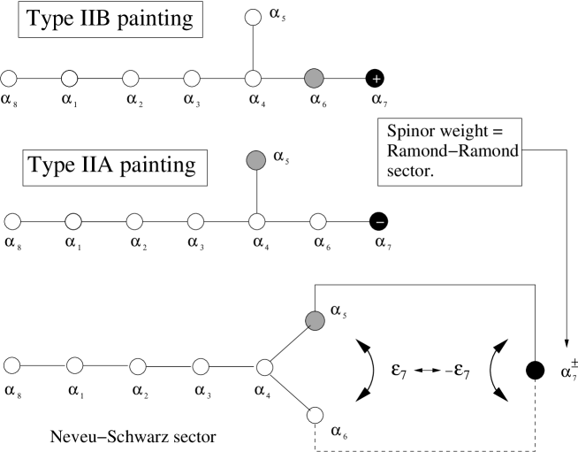
Figure 2: There are two different ways of embedding the $\mathrm{SL(7,R)}$ Lie algebra in $E_{8(8)}$ which correspond to the type II A and type II B interpretation of the same sigma model. This can also be seen as a different way of painting the same Dynkin diagram with blobs that are either associated with the metric (white) or with the $B$–field (gray) or with the Ramond–Ramond field (black). Furthermore the T–duality transforming the A painting into the B one is just the change in sign of the $\epsilon_{7}$ vector in Euclidean space. Indeed this corresponds, physically to inverting one of the torus radii $R_{9}\rightarrow\alpha^{\prime}/R_{9}$.

These two choices are illustrated in fig.2 where the roots belonging to the $SL(7,\mathbb{R})\subset GL(7,\mathbb{R})$ subgroup of the metric group are painted white. The roots eventually corresponding to a B–field are instead painted black, while the root eventually corresponding to a RR state are painted gray. As one sees the difference between the A and B interpretation of the same Dynkin diagram, named by us a painting of the same, resides in the fact that in the first case the RR root is linked to a metric, while in the second it is linked to a B–field.

In order to motivate the above identifications, let us start recalling that the $T^{7}$ metric–moduli parametrize the coset ${\mathcal{M}}^{A/B}_{g}\,=\,\mathrm{GL}(7,\mathbb{R})_{A/B}/\mathrm{SO(7)}$ in the type II A or B frameworks. If we describe ${\mathrm{\mathcal{M}}^{A/B}_{g}}$ as a solvable Lie group generated by the solvable Lie algebra $Solv({\mathcal{M}}^{A/B}_{g})$ [53, 22] then its coset representative $L^{p}{}_{\hat{q}}$ (in our notation the hatted indices are rigid, i.e. are acted on by the compact isotropy group) will be a solvable group element which, in virtue of the Iwasawa decomposition can be expressed as the product of a matrix ${\mathcal{N}}^{-1T}$, which is the exponent of a nilpotent matrix, times a diagonal one ${\mathcal{H}}^{-1}$: $L\,=\,{\mathcal{N}}^{-1T}\,{\mathcal{H}}^{-1}$. Indeed the matrix ${\mathcal{N}}^{-1T}$ is the exponential of the subalgebra $\mathcal{A}$ of $Solv({\mathcal{M}}^{A/B}_{g})$ spanned by the shift operators corresponding to the $\mathrm{GL}(7,\mathbb{R})_{A/B}$ positive roots, while ${\mathcal{H}}^{-1}$ is the exponential of the six–dimensional $\mathrm{GL}(7,\mathbb{R})_{A/B}$ Cartan subalgebra. The vielbein $E_{p}{}^{\hat{q}}$ corresponding to the $T^{7}$ metric $g_{pq}$ will have the following expression :

$$E = L^{-1T}\,=\,{\mathcal{N}}\,{\mathcal{H}}\,,$$

$$g = E\,E^{T}\,=\,{\mathcal{N}}\,{\mathcal{H}}\,{\mathcal{H}}^{T}\,{\mathcal{N}}^{T}\,.$$ (4.3)

The matrix ${\mathcal{N}}$ is non–trivial only if $T^{7}$ has off–diagonal metric–moduli. In the case of a straight torus, namely when $g_{pq}\,=\,e^{2\sigma_{p}}\,\delta_{pq}\,=\,R_{p}^{2}\,\delta_{pq}$ the diagonal entries of ${\mathcal{H}}$ are just the radii $R_{p}$: ${\mathcal{H}}_{p}{}^{\hat{q}}\,=\,R_{p}\,\delta_{p}{}^{\hat{q}}$.

The decomposition of $Solv(E_{8(8)}/SO(16))=Solv_{8}$ with respect to $Solv(GL(7,\mathbb{R})/SO(7))=Solv_{7}^{A/B}$ has the following form:

$$Solv_{8} = Solv_{7}^{A/B}+o(1,1)^{A/B}+{\mathcal{A}}^{[1]}+{\mathbf{B}}^{[1]}+{\mathbf{B}}^{[2]}+\sum_{k}{\mathbf{C}}_{A/B}^{[k]}$$ (4.4)

where $o(1,1)^{A/B}$ denote the Cartan generators $H_{\alpha[7]+\epsilon_{7}},\,H_{\alpha[7]}$, which are parametrized by the ten dimensional dilaton $\phi$ in the Type II A and II B settings respectively, ${\mathbf{B}}^{[2]}\,=\,B_{2+p\,,\,2+q}\,{\mathbf{B}}^{p\,\,q}$ is the subspace parametrized by the internal components of the Kalb–Ramond field and ${\mathbf{C}}_{A/B}^{[k]}\,=\,C_{2+p_{1}\,\dots\,2+p_{k}}\,{\mathbf{C}}^{p_{1}\,\dots\,p_{k}}$ the subspace spanned by the internal components of the R–R k–form (in our conventions $C_{2+p_{1},\dots 2+p_{k}}$ for $k>4$ are the dualized vectors $C_{2+q_{1}\,\dots\,2+q_{7-k},\mu}$, with $\epsilon^{p_{1}\dots p_{k}q_{1}\dots q_{7-k}}\,\neq\,0$). Finally the nilpotent spaces ${\mathcal{A}}^{[1]}$ and ${\mathbf{B}}^{[1]}$ are parametrized by the dualized Kaluza–Klein and Kalb–Ramon vectors: $g_{p\,\mu},\,B_{2+p,\,\mu}$. The nilpotent subspaces $\{{\mathcal{A}}^{[1]},\,{\mathbf{B}}^{[1]},\,{\mathbf{C}}_{A/B}^{[k]}\}$ define order–$k$ antisymmetric tensorial representations ${\mathbf{T}}^{[k]}\,=\,\{{\mathbf{T}}^{{p_{1}\dots p_{k}}}\}$ with respect to the adjoint action of $\mathrm{GL}(7,\mathbb{R})_{A/B}$:

$${\mathbf{E}} \in \mathrm{GL}(7,\mathbb{R})_{A/B}\,:\,\,\,{\mathbf{E}}\cdot{\mathbf{T}}^{{p_{1}\dots p_{k}}}\cdot{\mathbf{E}}^{-1}\,=\,E^{p_{1}}{}_{q_{1}}\dots E^{p_{k}}{}_{q_{k}}{\mathbf{T}}^{{q_{1}\dots q_{k}}}$$ (4.5)

From the definitions (4.2) we see that the shift generators in $Solv_{8}-Solv_{7}^{A}$ branch with respect to $\mathrm{GL}(7,\mathbb{R})_{A}$ into the subspaces ${\mathcal{A}}^{[1]},\,{\mathbf{B}}^{[1]},\,{\mathbf{B}}^{[2]}$ and ${\mathbf{C}}_{A}^{[k]}$, $k\,=\,1,\,3,\,5,\,7$ and those in $Solv_{8}-Solv_{7}^{B}$ branch with respect to $\mathrm{GL}(7,\mathbb{R})_{B}$ into ${\mathcal{A}}^{[1]},\,{\mathbf{B}}^{[1]},\,{\mathbf{B}}^{[2]}$ and ${\mathbf{C}}_{B}^{[k]}$, $k\,=\,0,\,2,\,4,\,6$. As far as the R–R scalars are concerned, these representations correspond indeed to the tensorial structure of the type II A spectrum $C_{2+p},\,C_{2+p\,,\,2+q\,,\,2+r},\,C_{\mu},\,C_{2+p\,,\,2+q\,,\,\mu}$ and type II B spectrum $C,\,C_{2+p,2+q},\,C_{2+p,2+q,2+r,2+s},\,C_{2+p,\mu}$. We can now define a one-to-one correspondence between axions and ${\mathrm{E}}_{8(8)}$ positive roots. The $T^{7}$ moduli space is ${\rm SO}(7,7)_{T}/[{\rm SO}(7)\times{\rm SO}(7)]\,=\,{\rm Exp}(Solv_{T})$ parametrized by the scalars $g_{2+p\,,\,2+q}$ and $B_{2+p\,,\,2+q}$, where:

$$Solv_{T} = Solv_{7}^{A/B}+{\mathbf{B}}^{[2]}$$ (4.6)

In three dimensions the scalar fields deriving from the dualization of $g_{p\mu}$ and $B_{p\,\mu}$ together with the dilaton $\phi$ enlarge the manifold ${\rm SO}(7,7)_{T}/[{\rm SO}(7)\times{\rm SO}(7)]$ to ${\rm SO}(8,8)/[{\rm SO}(8)\times{\rm SO}(8)]\,=\,{\rm Exp}(Solv_{NS})$ where now:

$$Solv_{NS} = Solv_{7}^{A/B}+o(1,1)+{\mathcal{A}}^{[1]}+{\mathbf{B}}^{[1]}+{\mathbf{B}}^{[2]}\,,$$ (4.7)

This manifold is parametrized by the 64 NS scalar fields. If we decompose $Solv_{8}$ with respect to $Solv_{NS}$ we may achieve an intrinsic group–theoretical characterization of the NS and R–R scalars. From this point of view the R–R scalar fields span the 64–dimensional subalgebra $Solv_{8}/Solv_{NS}$ which coincides with a spinorial representation of ${\rm SO}(7,7)_{T}$ with a definite chirality. Therefore the corresponding positive roots have grading one with respect to the ${\rm SO}(7,7)_{T}$ spinorial root $\alpha[7]$. Finally the higher–dimensional origin of the three dimensional scalar fields can be determined by decomposing $Solv_{8}$ with respect to the solvable algebra $Solv_{11-D}$ generating the scalar manifold ${\rm E}_{11-D(11-D)}/{\rm H}$ of the D–dimensional maximal supergravity. This decomposition is defined by the embedding of the higher–dimensional duality groups ${\rm E}_{11-D(11-D)}$ inside the three dimensional one. The Dynkin diagrams of the $E_{11-D(11-D)}$ nested Lie algebras are arranged according to the the pictures displayed in Fig. 3 and Fig. 4.

Figure 3: The Dynkin diagrams of $E_{3(3))}\subset E_{4(4)}\subset E_{5(5)}$ and the labeling of simple roots

Figure 4: The Dynkin diagrams of $E_{6(6))}\subset E_{7(7)}\subset E_{8(8)}$ and the labeling of simple roots

Let us now comment on the geometrical relation between the Type II A and II B representations. The two ${\rm SL}(7,\mathbb{R})_{A/B}$ Dynkin diagrams are mapped into each other by the ${\rm SO}(8,8)$ outer authomorphism $\epsilon_{7}\rightarrow-\epsilon_{7}$ which corresponds, in the light of our parametrization of the ${\rm E}_{8(8)}$ Cartan generators, to a T–duality along the direction $x^{9}$. This transformation defines the correspondence between the two inequivalent ${\rm SL}(8,\mathbb{R})_{A/B}$ inside which ${\rm SL}(7,\mathbb{R})_{A/B}$ are embedded. To show that this operation is indeed a T–duality (see [54] and also [55] for a geometrical definition of T–duality in the solvable Lie algebra formalism) let us recall the parametrization of the Cartan subalgebra in our setup:

Type II B:

$$\vec{h}\cdot\vec{H} = \sum_{p=1}^{7}\,\sigma_{p}\,(\epsilon_{p}-\epsilon_{8})-\frac{\phi}{2}\,\alpha_{7}\,=\,\sum_{p=1}^{7}\,\widetilde{\sigma}_{p}\,(\epsilon_{p}-\epsilon_{8})+2\phi\,\epsilon_{8}$$

Type II A:

$$\vec{h}\cdot\vec{H} = \sum_{p=1}^{7}\,\sigma_{p}\,(\epsilon^{\prime}_{p}-\epsilon^{\prime}_{8})-\frac{\phi}{2}\,(\alpha_{7}+\epsilon_{7})\,=\,\sum_{p=1}^{7}\,\widetilde{\sigma}_{p}\,(\epsilon^{\prime}_{p}-\epsilon^{\prime}_{8})+2\phi\,\epsilon^{\prime}_{8}$$ (4.8)

$$\epsilon^{\prime}_{w} = \epsilon_{w}\,,\,\,w\,\neq\,7\,,\,\,\,\epsilon^{\prime}_{7}\,=\,-\epsilon_{7}$$

where, in the case of a compactification on a straight torus, $\sigma_{p}\,=\,\log{(R_{p})}$ and $\widetilde{\sigma}_{p}\,=\,\log{(\widetilde{R}_{p})}$, $R_{p}$ and $\widetilde{R}_{p}$ being the $T^{7}$ radii in the ten–dimensional Einstein– or string–frame respectively. Let us consider a T–duality along directions $x^{i_{1}},\dots,\,x^{i_{k}}$: $\widetilde{R}_{i_{r}}\,\rightarrow\,1/\widetilde{R}_{i_{r}}$ ($r=1,\dots,k,\,\,\alpha^{\prime}\,=\,1$). The transformation $\epsilon_{i_{r}}\,\rightarrow\,-\epsilon_{i_{r}}$ in the expression of $\vec{h}\cdot\vec{H}$ can be absorbed by the transformation $\widetilde{\sigma}_{i_{r}}\,\rightarrow\,-\widetilde{\sigma}_{i_{r}}$ and $\phi\,\rightarrow\,\phi-\sum_{r=1}^{k}\,\widetilde{\sigma}_{i_{r}}$ which is indeed the effect of the T–duality.

As a result of this analysis the precise one–to–one correspondence between axions and positive roots can now be given in the following form:

Type II B:

$$C_{2+p_{1}\,\dots\,2+p_{k}}\,\leftrightarrow\,\alpha_{7}+\epsilon_{p_{1}}+\dots\epsilon_{p_{k}}\,,\,\,\,(k\,=\,2,\,4)\,,$$

$$C_{2+p\,,\,\mu}\,\leftrightarrow\,\alpha_{7}+\epsilon_{q_{1}}+\dots\epsilon_{q_{6}}\,,\,\,\,(\epsilon^{pq_{1}\dots q_{6}}\neq 0)\,,$$

$$B_{2+p\,,\,2+q}\,\leftrightarrow\,\epsilon_{p}+\epsilon_{q}\,,$$

$$B_{2+p\,,\,\mu}\,\leftrightarrow\,-\epsilon_{p}-\epsilon_{8}\,,$$

$$\gamma_{2+p}{}^{2+q}\,\leftrightarrow\,\epsilon_{p}-\epsilon_{q}$$

$$\gamma_{\mu}{}^{2+q}\,\leftrightarrow\,\epsilon_{q}-\epsilon_{8}$$

Type II A:

$$C_{2+p_{1}\dots 2+p_{k}}\,\leftrightarrow\,\alpha_{7}+\epsilon_{7}+\epsilon^{\prime}_{p_{1}}+\dots\epsilon^{\prime}_{p_{k}}\,,\,\,\,(k\,=\,1,\,3)\,,$$

$$C_{2+p_{1}\,,\,2+p_{2}\,,\,\mu}\,\leftrightarrow\,\alpha_{7}+\epsilon_{7}+\epsilon^{\prime}_{q_{1}}+\dots\epsilon^{\prime}_{q_{5}}\,,\,\,\,(\epsilon^{p_{1}p_{2}q_{1}\dots q_{5}}\neq 0)\,,$$

$$C_{\mu}\,\leftrightarrow\,\alpha_{7}+\epsilon_{7}+\epsilon^{\prime}_{1}+\dots\epsilon^{\prime}_{7}\,,$$

$$B_{2+p\,,\,2+q}\,\leftrightarrow\,\epsilon^{\prime}_{p}+\epsilon^{\prime}_{q}\,,$$

$$B_{2+p\,,\,\mu}\,\leftrightarrow\,-\epsilon^{\prime}_{p}-\epsilon^{\prime}_{8}\,,$$

$$\gamma_{2+p}{}^{2+q}\,\leftrightarrow\,\epsilon^{\prime}_{p}-\epsilon^{\prime}_{q}$$

$$\gamma_{\mu}{}^{2+q}\,\leftrightarrow\,\epsilon^{\prime}_{q}-\epsilon^{\prime}_{8}$$

where $\gamma_{2+p}{}^{2+q}$ are the parameters entering the matrix ${\mathcal{N}}$ and which determine the off–diagonal entries of the $T^{7}$ vielbein $E_{p}{}^{\hat{q}}$:

$$\mathcal{N} \equiv \exp{(\gamma_{2+p}{}^{2+q}\,\mathcal{A}_{q}{}^{p})}$$ (4.10)

for a precise definition of the above exponential representation see [53]. The fields $\gamma_{\mu}{}^{q}$ denote the scalars dual to the Kaluza–Klein vectors.

5 Oxidation of the $\mathrm{A_{2}}$ solutions

In this section, as a working illustration of the oxidation process we derive two full fledged $D=10$ supergravity backgrounds corresponding to the two $A_{2}$ sigma model solutions derived in previous sections. As we already emphasized in our introduction the correspondence is not one-to-one, rather it is one-to-many. This has two reasons. First of all we can either oxide to a type II A or to a type II B configuration. Secondly, even within the same supergravity choice (A or B), there are several different oxidations of the same abstract sigma model solution, just as many as the different ways of embedding the solvable $Solv(\mathrm{A_{2}})$ algebra into the solvable $Solv(\mathrm{E_{8}}/SO(16))$ algebra. This embeddings lead to quite different physical interpretations of the same abstract sigma model solution.

Our first task is the classification of these inequivalent embeddings.

5.1 Possible embeddings of the $A_{2}$ algebra

In order to study the possible embeddings it is convenient to rely on a compact notation and on the following graded structure of the Solvable Lie algebra $Solv(\mathrm{E_{8}}/SO(16))$ characterized by the following non vanishing commutators:

$$\left[\mathcal{A}\,,\,\mathcal{A}\right] = \mathcal{A}$$

$$\left[\mathcal{A}\,,\,\mathcal{A}^{[1]}\right] = \mathcal{A}^{[1]}$$

$$\left[\mathcal{A}\,,\,\mathbf{B}^{[1]}\right] = \mathbf{B}^{[1]}$$

$$\left[\mathcal{A}\,,\,\mathbf{B}^{[2]}\right] = \mathbf{B}^{[2]}$$

$$\left[\mathcal{A}\,,\,\mathbf{C}^{[k]}\right] = \mathbf{C}^{[k]}$$

$$\left[\mathbf{B}^{[2]}\,,\,\mathbf{B}^{[1]}\right] = \mathcal{A}^{[1]}$$

$$\left[\mathbf{B}^{[2]}\,,\,\mathbf{C}^{[k]}\right] = \mathbf{C}^{[k+2]}$$

$$\left[\mathbf{C}^{[k]}\,,\,\mathbf{C}^{[6-k]}\right] = {\mathbf{B}}^{[1]}$$

$$\left[\mathbf{C}^{[k]}\,,\,\mathbf{C}^{[8-k]}\right] = {\mathcal{A}}^{[1]}$$ (5.1)

In eq. (5.1) $\mathcal{A}^{[1]}$, $\mathbf{B}^{[2]}$, $\mathbf{B}^{[1]}$ and $\mathbf{C}^{[k]}$ are the spaces of nilpotent generators defined in the previous section, while $\mathcal{A}$ is the $Solv_{7}^{A/B}$ Lie algebra. In view of the above graded structure there are essentially $10$ physically different ways of embedding the $A_{2}$ algebra into $\mathrm{E_{8(8)}}$.

1

Every root $\beta_{1,2,3}$ is a metric generator ${\mathcal{A}}$. In this case the $A_{2}$ Lie algebra is embedded into the $\mathrm{SL(7,\mathbb{R})}$ subalgebra of $\mathrm{E_{8(8)}}$ and the corresponding oxidation leads to a purely gravitational background of supergravity which is identical in the type II A or type II B theory.

2

The root $\beta_{1}$ corresponds to an off–diagonal element of the internal metric, namely belongs to $\mathcal{A}$, while $\beta_{2,3}$ correspond to scalars dual to the Kaluza–Klein vectors $g_{2+p\,,\,\mu}$ namely belong to $\mathcal{A}^{[1]}$. This commutation relation follows from the fact that the $\mathcal{A}^{[1]}$ generators transform in the ${\bf 7}$ of $\mathrm{SL(7,\mathbb{R})}$.

3

The two simple roots $\beta_{1,2}$ are respectively associated with a metric generator ${\mathcal{A}}$ and a $B$-field generator $\mathbf{B}^{[1]}$ corresponding to the dualized vector field deriving from the Kalb–Ramond two form. The composite root $\beta_{3}$ is associated with a second $B$-field generator $\mathbf{B}^{[1]}$. This is so because the $\mathbf{B}^{[1]}$ transform in the ${\overline{7}}$ of $\mathrm{SL(7,\mathbb{R})}$. In this case oxidation leads to a purely NS configuration, shared by type II A and type II B theories, involving the metric, the dilaton and the B-field alone.

4

The two simple roots $\beta_{1,2}$ are respectively associated with a metric generator ${\mathcal{A}}$ and a $B$-field generator $\mathbf{B}^{[2]}$ parametrized by a $B_{pq}$ scalar field. The composite root $\beta_{3}$ is associated with a second $B$-field generator $\mathbf{B}^{[2]}$. This follows from the fact that $\mathbf{B}^{[2]}$ defines a representation ${\bf 21}$ of $\mathrm{SL(7,\mathbb{R})}$. In this case oxidation leads to a purely NS configuration, shared by type II A and type II B theories.

5

The two simple roots $\beta_{1,2}$ are respectively associated with a metric generator ${\mathcal{A}}$ and with a RR $k$–form generator $\mathbf{C}^{[k]}$. The composite root $\beta_{3}$ is associated with a second RR generator $\mathbf{C}^{[k]}$ in the same $[k]$–representation. This follows again from the fact that the $\mathbf{C}^{[k]}$ generators span an order –$k$ tensor representation of $\mathrm{SL(7,\mathbb{R})}$. In this case oxidation leads to different results in type II A and type II B theories, although the metric is the same for the two cases and it has non trivial off-diagonal parts.

6

The root $\beta_{1}$ is contained in $\mathbf{B}^{[2]}$, namely it describes an internal component of the B–field. The root $\beta_{2}\,\in\,\mathbf{B}^{[1]}$ namely it corresponds to a B–field with mixed indices. The root $\beta_{3}\,\in\,\mathcal{A}^{[1]}$ is associated with a Kaluza–Klein vector.

8

The simple roots $\beta_{1,2}$ are respectively associated with a RR $k$-form generator $\mathbf{C}^{[k]}$ and with a B-field generator $\mathbf{B}$. The composite root $\beta_{3}$ is associated with a $k+2$ form generator $\mathbf{C}^{{k+2}}$. In this case the metric is purely diagonal and we have non trivial B-fields and RR forms. Type II A and type II B oxidations are differ just in this latter sector. The NS sector is the same for both.

9

The two simple roots $\beta_{1,2}$ are respectively associated with a RR generator $\mathbf{C}^{[k]}$ and a RR generator $\mathbf{C}^{[6-k]}$. The composite root $\beta_{3}$ is associated with a $\mathbf{B}^{[1]}$ generator. The oxidation properties of this case are just similar to those of the previous case. Also here the metric is diagonal.

10

In type II B theory the roots $\beta_{1,2}$ belong to $C^{[k]}$ and $C^{[8-k]}$ namely are associated with the internal components of two different R–R forms, while $\beta_{3}\,\in\,\mathcal{A}^{[1]}$ describes a Kaluza–Klein vector.

5.2 Choice of one embedding example

As an illustration, out of the above list we choose one example of embedding that has an immediate and nice physical interpretation in terms of a brane system. We consider the case $4$, with a RR generator $\mathbf{C}^{[2]}$ and a B-field generator respectively associated with $\beta_{1,2}$ and a $\mathbf{C}^{[4]}$ generator associated with the composite root $\beta_{3}$. In particular we set:

$$\beta_{1} \rightarrow \mathbf{B}^{34}$$

$$\beta_{2} \rightarrow \mathbf{C}^{89}$$

$$\beta_{3} \rightarrow \mathbf{C}^{3489}\,\sim\,\mathbf{C}^{\mu 567}$$ (5.2)

More precisely this corresponds to identifying $\beta_{1,2,3}$ with the following roots of $E_{8(8)}$ according to their classification given in the appendix:

$$\begin{array}[]{cccclcc}\beta_{1}&\hookrightarrow&\alpha[69]&=&\epsilon_{1}+\epsilon_{2}&\leftrightarrow&B_{34}\\ \beta_{2}&\hookrightarrow&\alpha[15]&=&\alpha[7]+\epsilon_{6}+\epsilon_{7}&\leftrightarrow&C_{89}\\ \beta_{3}&\hookrightarrow&\alpha[80]&=&\alpha[7]+\epsilon_{1}+\epsilon_{1}+\epsilon_{6}+\epsilon_{7}&\leftrightarrow&C_{3489}\sim C_{\mu 567}\end{array}$$ (5.3)

where $\alpha[7]=\left\{-{\textstyle\frac{1}{2}},-{\textstyle\frac{1}{2}},-{\textstyle\frac{1}{2}},-{\textstyle\frac{1}{2}},-{\textstyle\frac{1}{2}},-{\textstyle\frac{1}{2}},-{\textstyle\frac{1}{2}},-{\textstyle\frac{1}{2}}\right\}$ is the spinorial simple root of $\mathrm{E_{8(8)}}$.

Next given the explicit form of the two roots $\beta_{1}\hookrightarrow\alpha[69]$ and $\beta_{2}\hookrightarrow\alpha[15]$ we construct the $2$–dimensional subspace of the Cartan subalgebra which is orthogonal to the orthogonal complement of $\alpha[69]$ and $\alpha[15]$ in $\mathbb{R}^{8}$. We immediately see that this subspace is spanned by all $8$ vectors of the form:

$$\overrightarrow{h}=\left\{x,x,y,y,y,-y,-y,y\right\}$$ (5.4)

so that we find:

$$\overrightarrow{h}\cdot\overrightarrow{\alpha}[69]=2x\quad;\quad\overrightarrow{h}\cdot\overrightarrow{\alpha}[15]=-(x+3y)$$ (5.5)

Then we relate the fields $x$ and $y$ to the diagonal part of the ten dimensional metric.

To this effect we start from the general relations between the ten-dimensional metric in the Einstein frame and the fields in three-dimensions evaluated in the $D=3$ Einstein frame, then we specialize such relations to our particular case.

General relations in dimensional reduction

The Einstein frame metric in $D=10$ can be written as:

$$G_{MN}^{(Einstein)}=\left(\begin{array}[]{c|c}\exp[4\phi_{3}-{\textstyle\frac{1}{2}}\phi]\,g^{(E,3)}_{\mu\nu}+G_{ij}\,\mathcal{A}^{i}_{\mu}\,\mathcal{A}^{i}_{\nu}&G_{ik}\,\mathcal{A}^{k}_{\mu}\\ \hline\cr G_{jk}\,\mathcal{A}^{k}_{\nu}&G_{ij}\end{array}\right)$$ (5.6)

where $g^{(E,3)}_{\mu\nu}$ is the three dimensional Einstein frame metric (2.10) determined by the solution of the $D=3$-sigma model via equations (2.17) and (2.18,2.19). On the other hand $G_{ij}$ is the Einstein frame metric in the internal seven directions. It parametrizes the coset:

$$\frac{\mathrm{GL(7,\mathbb{R})}}{\mathrm{SO(7)}}=O(1,1)\,\times\,\frac{\mathrm{SL(7,\mathbb{R})}}{\mathrm{SO(7)}}$$ (5.7)

In full generality, recalling eq.s(4.3) we can set ([53, 22]):

$$G=E\,E^{T}\quad;\quad E=\mathcal{N}\,\mathcal{H}$$ (5.8)

where, in this case:

$$\mathcal{N}_{ij}=\delta_{ij}$$ (5.9)

since there are no roots associated with metric generators, while the diagonal matrix:

$$H_{ij}=\exp[\sigma_{i}]\,\delta_{ij}$$ (5.10)

parametrizes the degrees of freedom associated with the Cartan subalgebra of $\mathrm{O(1,1)}\times\mathrm{SL(7,\mathbb{R})}$. The relation of the fields $\sigma_{i}$ with the dilaton field and the Cartan fields of $E_{8(8)}$ is obtained through the following general formulae:

$$\overrightarrow{h} = \sum_{p=1}^{7}\,\left(\sigma_{p}+{\textstyle\frac{1}{4}}\phi\right)\,\overrightarrow{\epsilon}_{p}+2\phi_{3}\,\overrightarrow{\epsilon}_{8}$$

$$\phi_{3} = {\textstyle\frac{1}{8}}\,\phi-{\textstyle\frac{1}{2}}\sum_{p=1}^{7}\,\sigma_{p}$$ (5.11)

$\phi$ being the dilaton in $D=10$ and $\phi_{3}$ its counterpart in $D=3$. The above formula follows immediately from eq.(4)

We also stress the following general property of the parametrization (5.6) for the $D=10$ metric:

$$\sqrt{-\mbox{det}G}\,G^{00}\,=\,\sqrt{-\mbox{det}g}\,\,g^{00}$$ (5.12)

having denoted $G$ the full Einstein metric in ten dimension and $g$ the Einstein metric in three dimension.

Specializing to our example

Hence, in our example the ansatz for $G_{ij}$ is diagonal

$$G_{ij}=\exp\left[2\sigma_{i}\right]\,\delta_{ij}\quad;\quad i=1,\dots,7$$ (5.13)

and we obtain the following relation between the fields $x$ and $y$ and the diagonal entries of the metric and the dilaton:

$$\phi=-\overrightarrow{h}\cdot\overrightarrow{\alpha}[7] = x+y$$

$$\sigma_{1,2} = \frac{3x-y}{4}$$

$$\sigma_{3,4,5} = \frac{3y-x}{4}$$

$$\sigma_{6,7} = -\frac{5y+x}{4}$$ (5.14)

Calling $\widetilde{h}_{1,2}$ the Cartan fields in the abstract $\mathrm{A_{2}}$ model discussed in section 3, we have:

$${\widetilde{h}}\cdot\beta_{1}=\sqrt{2}\,\widetilde{h}_{1}\quad;\quad{\widetilde{h}}\cdot\beta_{2}=-{\textstyle\frac{1}{\sqrt{2}}}\,\widetilde{h}_{1}\,+\,\sqrt{{\textstyle\frac{3}{2}}}\,\widetilde{h}_{2}$$ (5.15)

so that we can conclude:

$$x={\textstyle\frac{1}{\sqrt{2}}}\,\widetilde{h}_{1}\,\quad;\quad y=-{\textstyle\frac{1}{\sqrt{6}}}\widetilde{h}_{2}$$ (5.16)

We can also immediately conclude that:

$$Q^{2}=\frac{d}{dt}{h}\cdot\frac{d}{dt}{h}=\frac{d}{dt}{\widetilde{h}}\cdot\frac{d}{dt}{\widetilde{h}}=|\chi_{1}|^{2}+|\chi_{2}|^{2}$$ (5.17)

On the other hand the interpretation of $Q^{2}$ is the following. Consider the parameter $\varpi^{2}$ appearing in the three-dimensional metric determined from the sigma model by Einstein equations. It is defined as:

$$\varpi^{2}=h_{IJ}\dot{\phi}^{I}\,\dot{\phi}^{J}=\sum_{i=1}^{8}|\chi_{i}|^{2}+\sum_{\alpha=1}^{120}\,|\Phi|^{2}$$ (5.18)

If we calculate $\varpi^{2}$ using the generating solution or any other solution obtained from it by compensating $\mathrm{H}$-transformations, its value, which is a constant, does not change. So we have:

$$\varpi^{2}=\sum_{i=1}^{8}|\chi_{i}^{(\mbox{gen.sol.})}|^{2}$$ (5.19)

and in the lifting of our $\mathrm{A_{2}}$ solutions we can conclude that $Q^{2}=\varpi^{2}$. Let us calculate this crucial parameter for the case of the non trivial $A_{2}$ solutions discussed above. By means of straightforward algebra we get:

$$\varpi^{2}=|\chi_{1}^{(\mbox{gen.sol.})}|^{2}+|\chi_{2}^{(\mbox{gen.sol.})}|^{2}={\textstyle\frac{1}{24}}\,\left(\kappa^{2}+3\,\omega^{2}\right)$$ (5.20)

Next we turn to the identification of the $p$-forms. As we will explicitly verify by checking type II B supergravity field equations, the appropriately normalized identifications are the following ones:

$$B_{[2]} = \varphi_{1}(t)\,dx_{3}\,\wedge\,dx_{4}$$

$$C_{[2]} = \varphi_{2}(t)\,dx_{8}\,\wedge\,dx_{9}$$

$$C_{[4]} = \varphi_{3}(t)\,dx_{3}\,\wedge\,dx_{4}\,\wedge\,dx_{8}\,\wedge\,dx_{9}\,+\,U$$ (5.21)

where $U$ is the appropriate $4$–form needed to make the corresponding field strength self dual.

In this way recalling the normalizations of type II B field strengths as given in appendix we get:

$$F^{NS}_{[3]034} = {\textstyle\frac{1}{6}}\varphi_{1}\,^{\prime}(t)$$

$$F^{RR}_{[3]089} = {\textstyle\frac{1}{6}}\varphi_{2}\,^{\prime}(t)$$

$$F^{RR}_{[5]03489} = {\textstyle\frac{1}{240}}\,W(t)\,$$

$$F^{RR}_{[5]12567} = {\textstyle\frac{1}{240}}\,W(t)\,\sqrt{-\mbox{det}g}\,\frac{1}{g_{00}\,g_{33}\,g_{44}\,g_{88}\,g_{99}}$$ (5.22)

and we recognize that the combination $W(t)$ defined in eq.(3.28) is just the self-dual $5$-form field strength including Chern-Simons factors.

5.2.1 Full oxidation of the $A_{2}$ solution with only one root switched on

Let us now focus on the $A_{2}$ solution involving only the highest root (similar solutions were obtained in [56]-[60],[8]), namely on eq.s (3.47) and (3.48). Inserting the explicit form of the Cartan fields in eq.s(5.16) and then using (5.14) we obtain the complete form of the metric

$$ds^{2} = -r^{2}_{[0]}(t)\,dt^{2}+r^{2}_{[1|2]}(t)\,\left(dx_{1}^{2}+dx_{2}^{2}\right)+r^{2}_{[3|4]}(t)\,\left(dx_{3}^{2}+dx_{4}^{2}\right)$$ (5.23)

$$+r^{2}_{[5|6|7]}(t)\,\left(dx_{5}^{2}+dx_{6}^{2}+dx_{7}^{2}\right)+r^{2}_{[8|9]}(t)\,\left(dx_{8}^{2}+dx_{9}^{2}\right)$$

which is diagonal and it is parametrized by five time dependent scale factors

$$r^{2}_{[0]}(t) = e^{t\,{\sqrt{\frac{{\kappa}^{2}}{3}+{\omega}^{2}}}}\,{\sqrt{\cosh\frac{t\,\omega}{2}}}$$

$$r^{2}_{[1|2]}(t) = e^{\frac{t\,{\sqrt{\frac{{\kappa}^{2}}{3}+{\omega}^{2}}}}{2}}\,{\sqrt{\cosh\frac{t\,\omega}{2}}}$$

$$r^{2}_{[3|4]}(t) = \frac{1}{e^{\frac{t\,\kappa}{6}}\,{\sqrt{\cosh\frac{t\,\omega}{2}}}}$$

$$r^{2}_{[5|6|7]}(t) = {\sqrt{\cosh\frac{t\,\omega}{2}}}$$

$$r^{2}_{[8|9]}(t) = \frac{e^{\frac{t\,\kappa}{6}}}{{\sqrt{\cosh\frac{t\,\omega}{2}}}}$$ (5.24)

We also obtain the explicit form of the dilaton, which turns out to be linear in time:

$$\phi=-{\textstyle\frac{1}{6}}\,\kappa\,t$$ (5.25)

Calculating the Ricci tensor of the metric (5.23) we find that it is also diagonal and it has five independent eigenvalues respectively given by:

$$Ric_{00} = \frac{\left({\kappa}^{2}+9\,{\omega}^{2}+{\kappa}^{2}\,\cosh t\,\omega\right)\,{\mbox{sech}^{2}(\frac{t\,\omega}{2})}}{288}$$

$$Ric_{11}=Ric_{22} = \frac{{\omega}^{2}\,{\mbox{sech}^{2}(\frac{t\,\omega}{2})}}{32\,e^{\frac{t\,{\sqrt{\frac{{\kappa}^{2}}{3}+{\omega}^{2}}}}{2}}}$$

$$Ric_{33}=Ric_{44} = \frac{\omega^{2}\mbox{sech}^{2}(\frac{t\omega}{2})}{32\,e^{\frac{t\,{\sqrt{\frac{{\kappa}^{2}}{3}+{\omega}^{2}}}}{2}}}$$

$$Ric_{55}=Ric_{66}=Ric_{77} = \frac{-\omega^{2}\mbox{sech}^{3}(\frac{t\omega}{2})}{32\,e^{\frac{t\,\left(\kappa+6\,{\sqrt{\frac{{\kappa}^{2}}{3}+{\omega}^{2}}}\right)}{6}}}$$

$$Ric_{88}=Ric_{99} = \frac{-\omega^{2}\mbox{sech}^{3}(\frac{t\omega}{2})}{32\,e^{\frac{t\,\left(\kappa+6\,{\sqrt{\frac{{\kappa}^{2}}{3}+{\omega}^{2}}}\right)}{6}}}$$ (5.26)

On the other hand inserting the explicit values of scalar fields (3.48) into equations (5.21) we obtain:

$$F^{NS}_{[3]} = 0$$

$$F^{RR}_{[3]} = 0$$

$$F^{RR}_{[5]} = \frac{\omega\,{dt}\wedge{{{dx}}_{3}}\wedge{{{dx}}_{4}}\wedge{{{dx}}_{8}}\wedge{{{dx}}_{9}}}{1+\cosh t\,\omega}+\frac{\omega\,{{{dx}}_{1}}\wedge{{{dx}}_{2}}\wedge{{{dx}}_{5}}\wedge{{{dx}}_{6}}\wedge{{{dx}}_{7}}}{2}$$ (5.27)

Considering eq.s(5.27) and (5.25) together the physical interpretation of the parameters $\omega$ and $\kappa$ labeling the generating solution, becomes clear. They are respectively associated to the charges of the $D3$ and $D5$ branes which originate this classical supergravity solution. Indeed, as it is obvious from the last of eq.s (5.27), there is a dyonic $D3$-brane whose magnetic charge is uniformly distributed on the Euclidean hyperplane 12567 while the electric charge is attached to the Minkowskian hyperplane 03489. The magnetic charge per unit volume is $\omega/2$. With our choice of the $\mathrm{A_{2}}$ subalgebra, there should also be a $D5$-brane magnetically dual to an Euclidean $D$-string extending in the directions 89. In this particular solution, where $\varphi_{1,2}=0$ the $F^{RR}_{[3]}$ vanishes, yet the presence of the $D5$ brane is revealed by the dilaton. Indeed in a pure $D3$ brane solution the dilaton would be constant. The linear behaviour (5.25) of $\phi$, with coefficient $-\kappa/6$ is due to the $D5$ brane which couples non trivially to the dilaton field. Such an interpretation will become completely evident when we consider the oxidation of the solution obtained from this by a further $\mathrm{SO(3)}$ rotation which switches on all the roots. This we do in the next subsection. Then we will discuss how both oxidations do indeed satisfy the field equations of type II B supergravity and we will illustrate their physical properties as cosmic backgrounds.

5.2.2 Full oxidation of the $\mathrm{A_{2}}$ solution with all three roots switched on

Let us then turn to the $\mathrm{A_{2}}$ solution involving all the three nilpotent fields, namely to eq.s (3.51) and (3.52). Just as before, by inserting the explicit form of the Cartan fields in eq.s(5.16) and then using (5.14) we obtain the complete form of the new metric, which has the same diagonal structure as in the previous example, namely

$$ds^{2} = -\overline{r}^{2}_{[0]}(t)\,dt^{2}+\overline{r}^{2}_{[1|2]}(t)\,\left(dx_{1}^{2}+dx_{2}^{2}\right)+\overline{r}^{2}_{[3|4]}(t)\,\left(dx_{3}^{2}+dx_{4}^{2}\right)$$ (5.28)

$$+\overline{r}^{2}_{[5|6|7]}(t)\,\left(dx_{5}^{2}+dx_{6}^{2}+dx_{7}^{2}\right)+\overline{r}^{2}_{[8|9]}(t)\,\left(dx_{8}^{2}+dx_{9}^{2}\right)$$

now, however, the scale factors are given by:

$$\overline{r}^{2}_{[0]}(t) = e^{t\,\left(\frac{-\omega}{4}+{\sqrt{\frac{{\kappa}^{2}}{3}+{\omega}^{2}}}\right)}\,{\left(1+e^{t\,\omega}\right)}^{\frac{1}{4}}\,{\left(1+e^{t\,\omega}+e^{\frac{t\,\left(\kappa+\omega\right)}{2}}\right)}^{\frac{1}{4}}$$

$$\overline{r}^{2}_{[1|2]}(t) = e^{\frac{t\,\left(-3\,\omega+2\,{\sqrt{3}}\,{\sqrt{{\kappa}^{2}+3\,{\omega}^{2}}}\right)}{12}}\,{\left(1+e^{t\,\omega}\right)}^{\frac{1}{4}}\,{\left(1+e^{t\,\omega}+e^{\frac{t\,\left(\kappa+\omega\right)}{2}}\right)}^{\frac{1}{4}}$$

$$\overline{r}^{2}_{[3|4]}(t) = \frac{e^{\frac{-\left(t\,\kappa\right)}{6}+\frac{t\,\omega}{4}}\,{\left(1+e^{t\,\omega}+e^{\frac{t\,\left(\kappa+\omega\right)}{2}}\right)}^{\frac{1}{4}}}{{\left(1+e^{t\,\omega}\right)}^{\frac{3}{4}}}$$

$$\overline{r}^{2}_{[5|6|7]}(t) = \frac{{\left(1+e^{t\,\omega}\right)}^{\frac{1}{4}}\,{\left(1+e^{t\,\omega}+e^{\frac{t\,\left(\kappa+\omega\right)}{2}}\right)}^{\frac{1}{4}}}{e^{\frac{t\,\omega}{4}}}$$

$$\overline{r}^{2}_{[8|9]}(t) = \frac{e^{\frac{t\,\left(2\,\kappa+3\,\omega\right)}{12}}\,{\left(1+e^{t\,\omega}\right)}^{\frac{1}{4}}}{{\left(1+e^{t\,\omega}+e^{\frac{t\,\left(\kappa+\omega\right)}{2}}\right)}^{\frac{3}{4}}}$$ (5.29)

and the dilaton is no longer linear in time, rather it is given by:

$$\phi=\frac{-\left(t\,\kappa\right)-3\,\log(1+e^{t\,\omega})+3\,\log(1+e^{t\,\omega}+e^{\frac{t\,\left(\kappa+\omega\right)}{2}})}{6}$$ (5.30)

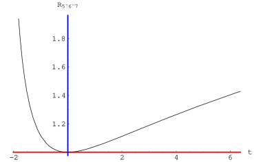
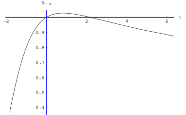
Figure 5: Plots of the scale factors $r^{2}_{[\alpha]}$, $\alpha=1|2\,,\,3|4\,,\,5|6|7\,,\,8|9$ as functions of the cosmic time $t=\tau(T)$ in the case of the choice of parameters $\omega=1$, $\kappa=0.5$ and for the $A_{2}$ solution with only the highest root switched on.

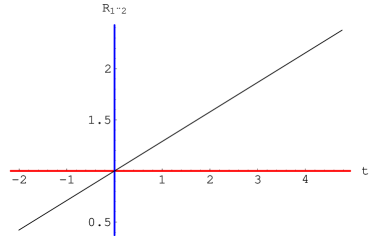
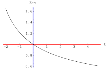
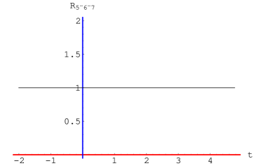
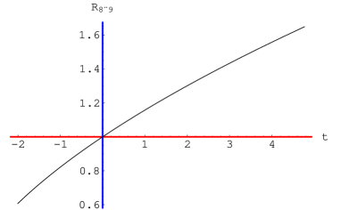
Figure 6: Plots of the scale factors $r^{2}_{[\alpha]}$, $\alpha=1|2\,,\,3|4\,,\,5|6|7\,,\,8|9$ as functions of the cosmic time $t=\tau(T)$ in the case of the choice of parameters $\omega=0$, $\kappa=1$ and for the $A_{2}$ solution with only the highest root switched on.

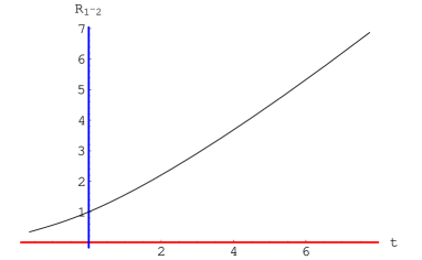
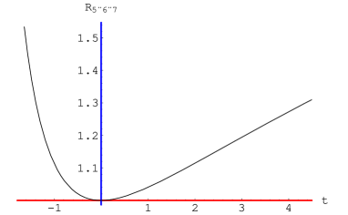
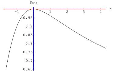
Figure 7: Plots of the scale factors $r^{2}_{[\alpha]}$, $\alpha=1|2\,,\,3|4\,,\,5|6|7\,,\,8|9$ as functions of the cosmic time $t=\tau(T)$ in the case of the choice of parameters $\omega=1$, $\kappa=0$ and for the $A_{2}$ solution with only the highest root switched on.

Calculating the Ricci tensor of the metric (5.28,5.29) we find it diagonal with five different eigenvalues, just as in the previous case, but with a modified time dependence, namely:

$$Ric_{00} = \frac{1}{576\,{\left(1+e^{t\,\omega}\right)}^{2}\,{\left(1+e^{t\,\omega}+e^{\frac{t\,\left(\kappa+\omega\right)}{2}}\right)}^{2}}\,\left({\left(1+e^{t\,\omega}\right)}^{2}\,\left(4+8\,e^{t\,\omega}+4\,e^{2\,t\,\omega}+23\,e^{\frac{t\,\left(\kappa+\omega\right)}{2}}\right.\right.$$

$$+\left.\left.e^{t\,\left(\kappa+\omega\right)}+23\,e^{\frac{t\,\left(\kappa+3\,\omega\right)}{2}}\right)\,{\kappa}^{2}-6\,e^{\frac{t\,\left(\kappa+\omega\right)}{2}}\,\left(-1+e^{2\,t\,\omega}\right)\,\left(7+7\,e^{t\,\omega}+e^{\frac{t\,\left(\kappa+\omega\right)}{2}}\right)\,\kappa\,\omega\right.$$

$$\left.+9\,\left(8\,e^{t\,\omega}+16\,e^{2\,t\,\omega}+8\,e^{3\,t\,\omega}+3\,e^{\frac{t\,\left(\kappa+\omega\right)}{2}}+e^{t\,\left(\kappa+\omega\right)}+10\,e^{t\,\left(\kappa+2\,\omega\right)}\right.\right.$$

$$\left.\left.+17\,e^{\frac{t\,\left(\kappa+3\,\omega\right)}{2}}+e^{t\,\left(\kappa+3\,\omega\right)}+17\,e^{\frac{t\,\left(\kappa+5\,\omega\right)}{2}}+3\,e^{\frac{t\,\left(\kappa+7\,\omega\right)}{2}}\right)\,{\omega}^{2}\right)$$

$$Ric_{11} = Ric_{22}$$

$$= \frac{1}{64\,{\left(1+e^{t\,\omega}\right)}^{2}\,{\left(1+e^{t\,\omega}+e^{\frac{t\,\left(\kappa+\omega\right)}{2}}\right)}^{2}}\,\left(e^{\frac{t\,\left(\omega-{\sqrt{\frac{{\kappa}^{2}}{3}+{\omega}^{2}}}\right)}{2}}\,\left(e^{\frac{t\,\left(\kappa+6\,\omega\right)}{2}}\,{\left(\kappa-\omega\right)}^{2}\right.\right.$$

$$\left.\left.+8\,e^{\frac{t\,\omega}{2}}\,{\omega}^{2}+16\,e^{\frac{3\,t\,\omega}{2}}\,{\omega}^{2}+8\,e^{\frac{5\,t\,\omega}{2}}\,{\omega}^{2}+4\,e^{t\,\left(\kappa+\frac{3\,\omega}{2}\right)}\,{\omega}^{2}\right.\right.$$

$$\left.\left.+e^{\frac{t\,\kappa}{2}}\,{\left(\kappa+\omega\right)}^{2}+e^{\frac{t\,\left(\kappa+4\,\omega\right)}{2}}\,\left(3\,{\kappa}^{2}-2\,\kappa\,\omega+11\,{\omega}^{2}\right)\right.\right.$$

$$\left.\left.+e^{\frac{t\,\kappa}{2}+t\,\omega}\,\left(3\,{\kappa}^{2}+2\,\kappa\,\omega+11\,{\omega}^{2}\right)\right)\right)$$

$$Ric_{33} = Ric_{44}$$

$$= \frac{1}{64\,e^{\frac{t\,\left(\kappa-6\,\omega+6\,{\sqrt{\frac{{\kappa}^{2}}{3}+{\omega}^{2}}}\right)}{6}}\,{\left(1+e^{t\,\omega}\right)}^{3}\,{\left(1+e^{t\,\omega}+e^{\frac{t\,\left(\kappa+\omega\right)}{2}}\right)}^{2}}\left(e^{\frac{t\,\left(\kappa+6\,\omega\right)}{2}}\,{\left(\kappa-\omega\right)}^{2}\right.$$

$$\left.-8\,e^{\frac{t\,\omega}{2}}\,{\omega}^{2}-16\,e^{\frac{3\,t\,\omega}{2}}\,{\omega}^{2}-8\,e^{\frac{5\,t\,\omega}{2}}\,{\omega}^{2}-12\,e^{t\,\left(\kappa+\frac{3\,\omega}{2}\right)}\,{\omega}^{2}\right.$$

$$\left.+e^{\frac{t\,\kappa}{2}}\,{\left(\kappa+\omega\right)}^{2}+e^{\frac{t\,\left(\kappa+4\,\omega\right)}{2}}\,\left(3\,{\kappa}^{2}-2\,\kappa\,\omega-21\,{\omega}^{2}\right)\right.$$

$$\left.+e^{\frac{t\,\kappa}{2}+t\,\omega}\,\left(3\,{\kappa}^{2}+2\,\kappa\,\omega-21\,{\omega}^{2}\right)\right)$$

$$Ric_{55} = Ric_{66}=Ric_{77}$$

$$= \frac{1}{64\,{\left(1+e^{t\,\omega}\right)}^{2}\,{\left(1+e^{t\,\omega}+e^{\frac{t\,\left(\kappa+\omega\right)}{2}}\right)}^{2}}\,\left(e^{\frac{t\,\left(\omega-2\,{\sqrt{\frac{{\kappa}^{2}}{3}+{\omega}^{2}}}\right)}{2}}\,\left(e^{\frac{t\,\left(\kappa+6\,\omega\right)}{2}}\,{\left(\kappa-\omega\right)}^{2}+8\,e^{\frac{t\,\omega}{2}}\,{\omega}^{2}+\right.\right.$$

$$\left.\left.16\,e^{\frac{3\,t\,\omega}{2}}\,{\omega}^{2}+8\,e^{\frac{5\,t\,\omega}{2}}\,{\omega}^{2}+4\,e^{t\,\left(\kappa+\frac{3\,\omega}{2}\right)}\,{\omega}^{2}+e^{\frac{t\,\kappa}{2}}\,{\left(\kappa+\omega\right)}^{2}\right.\right.$$

$$\left.\left.+e^{\frac{t\,\left(\kappa+4\,\omega\right)}{2}}\,\left(3\,{\kappa}^{2}-2\,\kappa\,\omega+11\,{\omega}^{2}\right)+e^{\frac{t\,\kappa}{2}+t\,\omega}\,\left(3\,{\kappa}^{2}+2\,\kappa\,\omega+11\,{\omega}^{2}\right)\right)\right)$$

$$Ric_{88} = Ric_{99}$$ (5.31)

$$= \frac{-1}{64\,{\left(1+e^{t\,\omega}\right)}^{2}\,{\left(1+e^{t\,\omega}+e^{\frac{t\,\left(\kappa+\omega\right)}{2}}\right)}^{3}}\,\left(e^{\frac{t\,\left(\kappa+6\,\omega-6\,{\sqrt{\frac{{\kappa}^{2}}{3}+{\omega}^{2}}}\right)}{6}}\,\left(3\,e^{\frac{t\,\left(\kappa+6\,\omega\right)}{2}}\,{\left(\kappa-\omega\right)}^{2}\right.\right.$$

$$\left.\left.+8\,e^{\frac{t\,\omega}{2}}\,{\omega}^{2}+16\,e^{\frac{3\,t\,\omega}{2}}\,{\omega}^{2}+8\,e^{\frac{5\,t\,\omega}{2}}\,{\omega}^{2}-4\,e^{t\,\left(\kappa+\frac{3\,\omega}{2}\right)}\,{\omega}^{2}+e^{\frac{t\,\left(\kappa+4\,\omega\right)}{2}}\,{\left(-3\,\kappa+\omega\right)}^{2}\right.\right.$$

$$\left.\left.+3\,e^{\frac{t\,\kappa}{2}}\,{\left(\kappa+\omega\right)}^{2}+e^{\frac{t\,\kappa}{2}+t\,\omega}\,{\left(3\,\kappa+\omega\right)}^{2}\right)\right)$$

On the other hand inserting the explicit values of scalar fields (3.52) into equations (5.21) we obtain:

$$F^{NS}_{[3]} = -{\textstyle\frac{1}{4}}\omega{\mbox{sech}^{2}(\frac{t\,\omega}{2})}dt\,\wedge\,dx_{3}\,\wedge\,dx_{4}$$

$$F^{RR}_{[3]} = \frac{e^{\frac{t\,\left(\kappa+\omega\right)}{2}}\,\left(\kappa+e^{t\,\omega}\,\left(\kappa-\omega\right)+\omega\right)}{2\,{\left(1+e^{t\,\omega}+e^{\frac{t\,\left(\kappa+\omega\right)}{2}}\right)}^{2}}\,dt\,\wedge\,dx_{8}\,\wedge\,dx_{9}$$

$$F^{RR}_{[5]} = \frac{e^{t\,\omega}\,\omega\,{dt}\wedge{{{dx}}_{3}}\wedge{{{dx}}_{4}}\wedge{{{dx}}_{8}}\wedge{{{dx}}_{9}}}{\left(1+e^{t\,\omega}\right)\,\left(1+e^{t\,\omega}+e^{\frac{t\,\left(\kappa+\omega\right)}{2}}\right)}-\omega\,{{{dx}}_{1}}\wedge{{{dx}}_{2}}\wedge{{{dx}}_{5}}\wedge{{{dx}}_{6}}\wedge{{{dx}}_{7}}$$ (5.32)

This formula completes the oxidation also of the second sigma model solution to a full fledged $D=10$ type II B configuration. As expected in both cases the ten dimensional fields obtained by oxidation satisfy the field equations of supergravity as formulated in the appendix (see eq.s(B.4)-(B.9)). We discuss this in the next section.

5.2.3 How the supergravity field equations are satisfied and their cosmological interpretation

Taking into account that the Ramond scalar $C_{0}$ vanishes the effective bosonic field equations of supergravity reduce to:

$$d\star d\phi = {\textstyle\frac{1}{2}}\left(e^{-\phi}\,F_{3}^{NS}\wedge\star F_{3}^{NS}-e^{\phi}\,F_{3}^{RR}\wedge\star F_{3}^{RR}\right)$$ (5.33)

$$0 = F_{3}^{NS}\wedge\star F_{3}^{NS}$$ (5.34)

$$d\left(e^{-\phi}F_{3}^{NS}\right) = -F_{3}^{RR}\wedge\star F_{5}^{RR}$$ (5.35)

$$d\left(e^{\phi}F_{3}^{RR}\right) = F_{3}^{NS}\wedge\star F_{5}^{RR}$$ (5.36)

$$d\left(\star F_{3}^{RR}\right) = -F_{3}^{NS}\wedge F_{3}^{RR}$$ (5.37)

$$-2Ric_{MN} = \hat{T}_{MN}$$ (5.38)

where the reduced stress energy tensor $\hat{T}_{MN}$ is the superposition of two contributions that we respectively attribute to the $D3$ brane and to the $D5$-brane, namely:

$$\hat{T}_{MN} = \hat{T}_{MN}^{[D3]}+\hat{T}_{MN}^{[D5]}$$ (5.39)

$$\hat{T}_{MN}^{[D3]} \equiv 150{F}_{[5]{M}\cdot\cdot\cdot\cdot}{F}_{[5]{N}}^{\phantom{{M}}\cdot\cdot\cdot\cdot}$$ (5.40)

$$\hat{T}_{MN}^{[D5]} \equiv \frac{1}{2}\partial_{{M}}\varphi\partial_{{N}}\varphi+9\left(e^{-\varphi}F_{[3]{M}\cdot\cdot}^{NS}\,F_{[3]{N}}^{{NS}\phantom{{M}}\cdot\cdot}+e^{\varphi}{F}_{[3]{M}\cdot\cdot}^{RR}{F}_{[3]{N}}^{RR\phantom{{M}}\cdot\cdot}\right)$$ (5.41)

$$-\frac{3}{4}\,g_{{MN}}\,\left(e^{-\varphi}F_{[3]\cdot\cdot\cdot}^{NS}F_{[3]}^{NS\cdot\cdot\cdot}+e^{\varphi}{{F}}_{[3]\cdot\cdot\cdot}^{RR}{F}^{RR\cdot\cdot\cdot}_{[3]}\right)$$

By means of laborious algebraic manipulations that can be easily performed on a computer with the help of MATHEMATICA, we have explicitly verified that in both cases, that of section 5.2.1 and that of section 5.2.2 the field eq.s(5.33)-(5.38) are indeed satisfied, so that the oxidation procedure we have described turns out to be well tuned and fully correct.

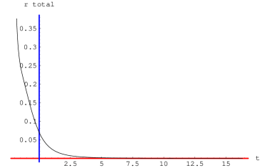
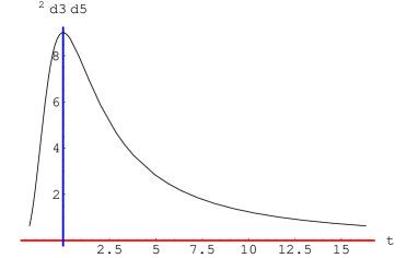
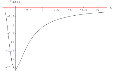
Figure 8: Plots of the energy densities in the case of the choice of parameters $\omega=1$, $\kappa=0.5$ and for the $A_{2}$ solution with only the highest root switched on. The first picture plots the total density $\rho^{tot}(\tau)$. The second picture plots the ratio $\rho^{d3}(\tau)/\rho^{tot}(\tau)$ and the third plots the ratio $\rho^{d3}(\tau)/\rho^{d5}(\tau)$

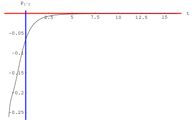
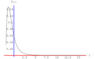
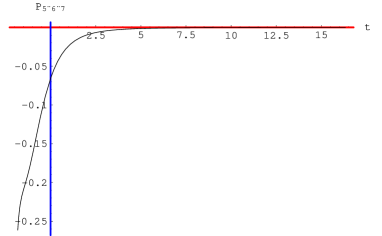
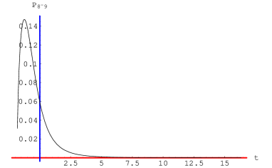
Figure 9: Plots of the pressure eigenvalues $P_{[\alpha]}$, $\alpha=1|2\,,\,3|4\,,\,5|6|7\,,\,8|9$ as functions of the cosmic time $t=\tau(T)$ in the case of the choice of parameters $\omega=1$, $\kappa=0.5$ and for the $A_{2}$ solution with only the highest root switched on.

In order to enlighten the physical meaning of the type II B superstring backgrounds we have eventually constructed it is worth to analyze the structure of the stress energy tensor. First, reintroducing the missing traces we define:

$$T_{MN}^{[D3]} = \hat{T}_{MN}^{[D3]}-{\textstyle\frac{1}{2}}\,g_{MN}\,\hat{T}_{RS}^{[D3]}\,g^{RS}$$

$$T_{MN}^{[D5]} = \hat{T}_{MN}^{[D5]}-{\textstyle\frac{1}{2}}\,g_{MN}\,\hat{T}_{RS}^{[D5]}\,g^{RS}$$

$$T_{MN}^{tot} = T_{MN}^{[D3]}+T_{MN}^{[D5]}$$ (5.42)

It turns out that the stress energy tensors are diagonal, just as the metric, and have the form of a perfect fluid, but with different pressure eigenvalues in the various subspaces. Indeed we can write:

$$T_{00}^{tot,\,D3,\,D5} = g_{00}\,\rho^{tot,\,D3,\,D5}$$

$$T_{i_{\alpha}j_{\alpha}}^{tot,\,D3,\,D5} = -g_{i_{\alpha}j_{\alpha}}\,P_{\alpha}^{tot,\,D3,\,D5}$$ (5.43)

where $\alpha$ denotes the four different submanifolds extending in directions:

$$\alpha=1|2\,,\,3|4\,,\,5|6|7\,,\,8|9$$ (5.44)

We can now analyze the specific properties of the two example of solutions.

5.2.4 Properties of the solution with just one root switched on

In the case of the time dependent background described in section (5.2.1) and obtained by oxiding the solution (3.48) we obtain for the energy densities:

$$\rho^{tot} = \frac{{\left(1+e^{t\,\omega}\right)}^{2}\,{\kappa}^{2}+9\,e^{t\,\omega}\,{\omega}^{2}}{36\,e^{t\,{\sqrt{\frac{{\kappa}^{2}}{3}+{\omega}^{2}}}}\,{\left(1+e^{t\,\omega}\right)}^{2}\,{\sqrt{\cosh\frac{t\,\omega}{2}}}}$$

$$\rho^{d3} = \frac{{\omega}^{2}}{16\,e^{t\,{\sqrt{\frac{{\kappa}^{2}}{3}+{\omega}^{2}}}}\,{\cosh^{\frac{5}{2}}\frac{t\,\omega}{2}}}$$

$$\rho^{d5} = \frac{{\kappa}^{2}}{36\,e^{t\,{\sqrt{\frac{{\kappa}^{2}}{3}+{\omega}^{2}}}}\,{\sqrt{\cosh\frac{t\,\omega}{2}}}}$$ (5.45)

for the total pressures:

$$P_{1|2}^{tot} = -\frac{\kappa^{2}+9\omega^{2}+\kappa^{2}\cosh t\omega}{144e^{t\sqrt{\frac{\kappa^{2}}{3}+\omega^{2}}}\cosh^{\frac{5}{2}}\frac{t\omega}{2}}$$

$$P_{3|4}^{tot} = -\frac{e^{t\left(\omega-\sqrt{\frac{\kappa^{2}}{3}+\omega^{2}}\right)}\left(\kappa^{2}-9\omega^{2}+\kappa^{2}\cosh t\omega\right)}{36{\left(1+e^{t\omega}\right)}^{2}\sqrt{\cosh\frac{t\omega}{2}}}$$

$$P_{5|6|7}^{tot} = -\frac{\kappa^{2}+9\omega^{2}+\kappa^{2}\cosh t\omega}{144e^{t\sqrt{\frac{\kappa^{2}}{3}+\omega^{2}}}\cosh^{\frac{5}{2}}\frac{t\omega}{2}}$$

$$P_{8|9}^{tot} = -\frac{e^{t\left(\omega-\sqrt{\frac{\kappa^{2}}{3}+\omega^{2}}\right)}\left(\kappa^{2}-9\omega^{2}+\kappa^{2}\cosh t\omega\right)}{36\left(1+e^{t\omega}\right)^{2}\sqrt{\cosh\frac{t\omega}{2}}}$$ (5.46)

for the pressures associated with the $D3$ brane:

$$P_{1|2}^{D3} = \frac{-{\omega}^{2}}{16\,e^{t\,{\sqrt{\frac{{\kappa}^{2}}{3}+{\omega}^{2}}}}\,{\cosh^{\frac{5}{2}}\frac{t\omega}{2}}}$$

$$P_{3|4}^{D3} = \frac{{\omega}^{2}}{16\,e^{t\,{\sqrt{\frac{{\kappa}^{2}}{3}+{\omega}^{2}}}}\,{\cosh^{\frac{5}{2}}\frac{t\omega}{2}}}$$

$$P_{5|6|7}^{D3} = \frac{-{\omega}^{2}}{16\,e^{t\,{\sqrt{\frac{{\kappa}^{2}}{3}+{\omega}^{2}}}}\,{\cosh^{\frac{5}{2}}\frac{t\,\omega}{2}}}$$

$$P_{8|9}^{D3} = \frac{{\omega}^{2}}{16\,e^{t\,{\sqrt{\frac{{\kappa}^{2}}{3}+{\omega}^{2}}}}\,{\cosh^{\frac{5}{2}}\frac{t\,\omega}{2}}}$$ (5.47)

and for the pressures associated with the $D5$ brane:

$$P_{1|2}^{D5} = \frac{-{\kappa}^{2}}{72\,e^{t\,{\sqrt{\frac{{\kappa}^{2}}{3}+{\omega}^{2}}}}\,{\sqrt{\cosh\frac{t\,\omega}{2}}}}$$

$$P_{3|4}^{D5} = \frac{-{\kappa}^{2}}{72\,e^{t\,{\sqrt{\frac{{\kappa}^{2}}{3}+{\omega}^{2}}}}\,{\sqrt{\cosh\frac{t\,\omega}{2}}}}$$

$$P_{5|6|7}^{D5} = \frac{-{\kappa}^{2}}{72\,e^{t\,{\sqrt{\frac{{\kappa}^{2}}{3}+{\omega}^{2}}}}\,{\sqrt{\cosh\frac{t\,\omega}{2}}}}$$

$$P_{8|9}^{D5} = \frac{-{\kappa}^{2}}{72\,e^{t\,{\sqrt{\frac{{\kappa}^{2}}{3}+{\omega}^{2}}}}\,{\sqrt{\cosh\frac{t\,\omega}{2}}}}$$ (5.48)

As we see from its analytic expression the total energy density is an exponentially decreasing function of time which tends to zero at asymptotically late times ($t\mapsto\infty$). What happens instead at asymptotically early times ($t\mapsto-\infty$) depends on the value of $\kappa$. For $\kappa=0$ we have $\lim_{t\mapsto-\infty}\rho^{tot}(t)=0$, while for $\kappa\neq 0$ we always have $\lim_{t\mapsto-\infty}\rho^{tot}(t)=\infty$. This is illustrated, for instance, in figs.(8) and (10). This phenomenon is related to the presence or absence of a $D5$ brane as it is evident from eq.s (5.45) which shows that the dilaton-($D5$) brane contribution to the energy density is proportional to $\kappa^{2}$ and it is always divergent at asymptotically early times, while the $D3$ brane contribution tends to zero in the same regime.

We also note, comparing eq.s(5.48) with eq.s(5.47) that the pressure contributed by the dilaton–$D5$–brane system is the same in all directions 1–9, while the pressure contributed by the $D3$–brane system is just opposite in the direction 3489 and in the transverse directions 12567. This is the origin of the cosmic billiard phenomenon that we observe in the behaviour of the metric scale factors. Indeed the presence of the $D3$-brane causes, at a certain instant of time, a switch in the cosmic expansion. Dimensions that were previously shrinking begin to expand and dimensions that were expanding begin to shrink. It is like a ball that hits a wall and inverts its speed. In the exact solution that we have constructed through reduction to three dimensions this occurs in a smooth way. There is a maximum and respectively a minimum in the behaviour of certain scale factors, which is in relation with a predominance of the $D3$–brane energy density with respect to the total energy density. The cosmic $D3$–brane behaves just as an instanton. Its contribution to the total energy is originally almost zero, then it raises and dominates for some time, then it exponentially decays again. This is the smooth exact realization of the potential walls envisaged by Damour et al.

To appreciate such a behaviour it is convenient to consider some plots of the scale factors, the energy densities and the pressures. In order to present such plots we first reduce the metric (5.23) to a standard cosmological form, by introducing a new time variable $\tau$ such that:

$$r_{[0]}(t)\,dt=d\tau$$ (5.49)

Explicitly we set:

$$\tau=\int_{0}^{T}\,r_{[0]}(t)\,dt$$ (5.50)

and inserting the explicit form of the scale factor $r_{[0]}(t)$ as given in eq.(5.24) we obtain:

$$\tau(T) = \frac{4\,2^{\frac{3}{4}}}{\omega-4\,{\sqrt{\frac{{\kappa}^{2}}{3}+{\omega}^{2}}}}\,\left[{{}_{2}F_{1}}\left(-{\textstyle\frac{1}{8}}+{\textstyle\frac{{\sqrt{\frac{{\kappa}^{2}}{3}+{\omega}^{2}}}}{2\,\omega}},-{\textstyle\frac{1}{4}},{\textstyle\frac{7}{8}}+{\textstyle\frac{{\sqrt{\frac{{\kappa}^{2}}{3}+{\omega}^{2}}}}{2\,\omega}},-1\right)\right.$$ (5.51)

$$\left.-e^{\frac{T\,\left(-\omega+4\,{\sqrt{\frac{{\kappa}^{2}}{3}+{\omega}^{2}}}\right)}{8}}\,{{}_{2}F_{1}}\left(-{\textstyle\frac{1}{8}}+{\textstyle\frac{{\sqrt{\frac{{\kappa}^{2}}{3}+{\omega}^{2}}}}{2\,\omega}},-{\textstyle\frac{1}{4}},{\textstyle\frac{7}{8}}+{\textstyle\frac{{\sqrt{\frac{{\kappa}^{2}}{3}+{\omega}^{2}}}}{2\,\omega}},-e^{T\,\omega}\right)\right]$$

which expresses $\tau$ in terms of hypergeometric functions and exponentials.

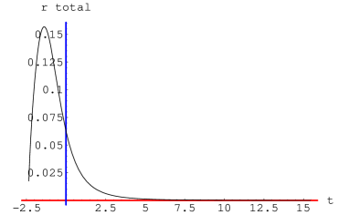
Figure 10: Plot of the energy density as function of the cosmic time $t=\tau(T)$ in the case of a pure $D3$ brane system, namely for the the choice of parameters $\omega=1$, $\kappa=0$ and for the $A_{2}$ solution with only the highest root switched on.

In fig.(5) we observe the billiard phenomenon in a generic case where both parameters $\omega$ and $\kappa$ are non vanishing. Since the value of $\omega$ can always be rescaled by a rescaling of the original time coordinate $t$, we can just set it to $1$ and what matters is to distinguish the case $\omega\neq 0$ where the $D3$ brane is present from the case $\omega=0$ corresponding to its absence. Hence fig.(5) corresponds to the presence of both a $D3$–brane and a dilaton–$D5$–brane system. A very different behavior occurs in fig.(6) where $\omega=0$. In this case there is no billiard and the dimensions either shrink or expand uniformly. On the other hand in fig.(7) we observe the pure billiard phenomenon induced by the $D3$-brane in the case where no dilaton-$D5$–brane is present, namely when we set $\kappa=0$. In this case, as we see, the parallel directions to the Euclidean $D3$–brane, namely 3489 have exactly the same behaviour: they first inflate and then they deflate, namely there is a maximum in the scale factor. The transverse directions to the $D3$ brane 567 have the opposite behaviour. They display a minimum at the same point where the parallel directions display a maximum. In all cases the directions 12 corresponding to the spatial directions of the three dimensional sigma model world suffer a uniform expansion.

Let us now consider the behavior of the energy densities. In fig.(8) we focus on the mixed case $\omega=1$, $\kappa=0.5$ characterized by the presence of both a $D3$ brane and dilaton-$D5$–brane system. As we see the total energy density exponentially decreases at late times and has a singularity at asymptotically early times. This is like in a standard Big Bang cosmological model with an indefinite expansion starting from an initial singularity. Yet the ratio of the $D3$ energy with respect to the total energy has a maximum at some instant of time and this is the cause of the billiard phenomenon in the behaviour of the scale factors respectively parallel and transverse to the $D3$ brane itself. The two contributions to the energy density from the $D3$–brane and from the dilaton have the same sign and the plot of their ratio displays a maximum in correspondence with the billiard time. With the same choice of parameters $\omega=1$, $\kappa=0.5$ the physical behavior of the system can be appreciated by looking at the plots of the pressure eigenvalues. They are displayed in fig.(9). We observe that the pressure is negative in the directions transverse to the $D3$ brane 12 and 567. Slowly, but uniformly it increases to zero in these directions. In the directions parallel to the brane the pressure is instead always positive and it displays a sharp maximum at the instant of time where the billiard phenomenon occurs.

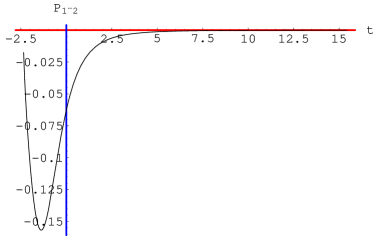
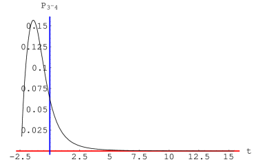
Figure 11: Plots of the pressure eigenvalues $P_{[\alpha]}$, $\alpha=1|2\,,\,3|4\,,\,5|6|7\,,\,8|9$ as functions of the cosmic time $t=\tau(T)$ in the case of the choice of parameters $\omega=1$, $\kappa=0$ and for the $A_{2}$ solution with only the highest root switched on. This case corresponds to a pure $D3$ brane system.

For a pure $D3$ brane system, namely for $\kappa=0$ and $\omega=1$ the energy density starts at zero, develops a maximum and then decays again to zero. This can be seen in fig.(10). The plot of the pressures is displayed, for this case in fig.(11). In this case the pressure in the directions transverse to the brane, i.e. 12567 is negative and it is just the opposite of the pressure in the directions parallel to the brane, namely 3489. This behavior causes the corresponding scale factors to suffer a minimum and a maximum, respectively.

5.2.5 Properties of the solution with all roots switched on

Let us now discuss the properties of the second solution where all the roots have been excited. In section 5.2.2 we considered the oxidation of such a sigma model solution and we constructed the corresponding $D=10$ supergravity background given by the metric (5.28, 5.29) and by the field strengths (5.32). Looking at eq.s (5.32) we see that the interpretation of the parameter $\omega$ is still the same as it was before, namely it represents the magnetic charge of the dyonic $D3$-brane. At $\omega=0$ the $D3$–brane disappears. Yet it appears from eq.s (5.32) that there is no obvious interpretation of the parameter $\kappa$ as a pure $D5$-brane charge. Indeed there is no choice of $\kappa$ which suppresses both the NS and the RR $3$–form field strengths.

Following the same procedure as in the previous case we calculate the energy density and the pressures and we separate the contributions due to the $D3$–brane and to the dilaton–$D5$–brane system. After straightforward but lengthy algebraic manipulations, implemented on a computer with MATHEMATICA we obtain:

$$\rho^{tot} = \frac{e^{t\,\left(\frac{\omega}{4}-{\sqrt{\frac{{\kappa}^{2}}{3}+{\omega}^{2}}}\right)}\,}{192\,{\left(1+e^{t\,\omega}\right)}^{\frac{9}{4}}\,{\left(1+e^{t\,\omega}+e^{\frac{t\,\left(\kappa+\omega\right)}{2}}\right)}^{\frac{9}{4}}}\,\left[{\left(1+e^{t\,\omega}\right)}^{2}\,\left(4+8\,e^{t\,\omega}+4\,e^{2\,t\,\omega}\right.\right.$$

$$\left.\left.+20\,e^{\frac{t\,\left(\kappa+\omega\right)}{2}}+e^{t\,\left(\kappa+\omega\right)}+20\,e^{\frac{t\,\left(\kappa+3\,\omega\right)}{2}}\right)\,{\kappa}^{2}\right.$$

$$\left.-6\,e^{\frac{t\,\left(\kappa+\omega\right)}{2}}\,\left(-1+e^{2\,t\,\omega}\right)\,\left(6+6\,e^{t\,\omega}+e^{\frac{t\,\left(\kappa+\omega\right)}{2}}\right)\,\kappa\,\omega\right.$$

$$\left.+3\,\left(16\,e^{t\,\omega}+32\,e^{2\,t\,\omega}+16\,e^{3\,t\,\omega}+8\,e^{\frac{t\,\left(\kappa+\omega\right)}{2}}+3\,e^{t\,\left(\kappa+\omega\right)}\right.\right.$$

$$\left.\left.+26\,e^{t\,\left(\kappa+2\,\omega\right)}+40\,e^{\frac{t\,\left(\kappa+3\,\omega\right)}{2}}+3\,e^{t\,\left(\kappa+3\,\omega\right)}+40\,e^{\frac{t\,\left(\kappa+5\,\omega\right)}{2}}+8\,e^{\frac{t\,\left(\kappa+7\,\omega\right)}{2}}\right)\,{\omega}^{2}\right]$$

$$\rho^{d3} = \frac{{\omega}^{2}}{4\,e^{t\,\left(\frac{-5\,\omega}{4}+{\sqrt{\frac{{\kappa}^{2}}{3}+{\omega}^{2}}}\right)}\,{\left(1+e^{t\,\omega}\right)}^{\frac{5}{4}}\,{\left(1+e^{t\,\omega}+e^{\frac{t\,\left(\kappa+\omega\right)}{2}}\right)}^{\frac{5}{4}}}$$

$$\rho^{d5} = \frac{e^{t\,\left(\frac{\omega}{4}-{\sqrt{\frac{{\kappa}^{2}}{3}+{\omega}^{2}}}\right)}\,}{192\,{\left(1+e^{t\,\omega}\right)}^{\frac{9}{4}}\,{\left(1+e^{t\,\omega}+e^{\frac{t\,\left(\kappa+\omega\right)}{2}}\right)}^{\frac{9}{4}}}\,\left[{\left(1+e^{t\,\omega}\right)}^{2}\,\left(4+8\,e^{t\,\omega}+4\,e^{2\,t\,\omega}+20\,e^{\frac{t\,\left(\kappa+\omega\right)}{2}}\right.\right.$$ (5.52)

$$\left.\left.+e^{t\,\left(\kappa+\omega\right)}+20\,e^{\frac{t\,\left(\kappa+3\,\omega\right)}{2}}\right)\,{\kappa}^{2}\right.$$

$$\left.-6\,e^{\frac{t\,\left(\kappa+\omega\right)}{2}}\,\left(-1+e^{2\,t\,\omega}\right)\,\left(6+6\,e^{t\,\omega}+e^{\frac{t\,\left(\kappa+\omega\right)}{2}}\right)\,\kappa\,\omega\right.$$

$$\left.+3\,\left(8\,e^{\frac{t\,\left(\kappa+\omega\right)}{2}}+3\,e^{t\,\left(\kappa+\omega\right)}+26\,e^{t\,\left(\kappa+2\,\omega\right)}+24\,e^{\frac{t\,\left(\kappa+3\,\omega\right)}{2}}\right.\right.$$

$$\left.\left.+3\,e^{t\,\left(\kappa+3\,\omega\right)}+24\,e^{\frac{t\,\left(\kappa+5\,\omega\right)}{2}}+8\,e^{\frac{t\,\left(\kappa+7\,\omega\right)}{2}}\right)\,{\omega}^{2}\right]$$

We see from the above formulae that the energy density contributed by the $D3$–brane system is proportional to $\omega^{2}$ as before and vanishes at $\omega=0$. However there is no choice of the parameter $\kappa$ which suppresses the dilaton–$D5$–contribution leaving the $D3$–contribution non–zero.

The pressure eigenvalues can also be calculated just as in the previous example but the resulting analytic formulae are quite messy and we do not feel them worthy to be displayed. It is rather convenient to consider a few more plots.

Just as in the previous case we define the cosmic time through the formula (5.50). In this case, however, the integral does not lead to a closed formula in terms of special functions and we just have an implicit definition:

$$\tau(T)\,\equiv\,\int_{0}^{T}\,e^{\frac{t\,\left(\frac{-\omega}{4}+{\sqrt{\frac{{\kappa}^{2}}{3}+{\omega}^{2}}}\right)}{2}}\,{\left(1+e^{t\,\omega}\right)}^{\frac{1}{8}}\,{\left(1+e^{t\,\omega}+e^{\frac{t\,\left(\kappa+\omega\right)}{2}}\right)}^{\frac{1}{8}}\,dt$$ (5.53)

Let us now observe from eq.s (5.29), (5.32) that there are the following critical values of the parameters:

1

For $\omega=0$ and $\kappa\neq 0$ there is no $D3$–brane and there is just a $D$–string dual to a $D5$–brane.

2

For $\kappa=\pm{\textstyle\frac{3}{2}}\,\omega$ the scale factor in the directions 34 tends to a finite asymptotic value respectively at very early or very late times.

The plot of the scale factors for the choice $\omega=0$, $\kappa=3/2$ is given in fig.(12)

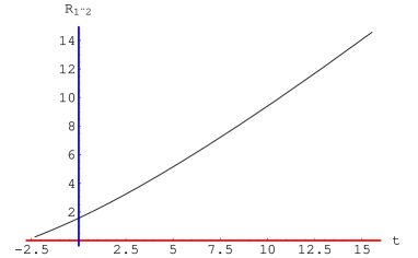
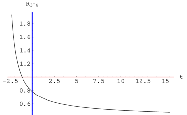
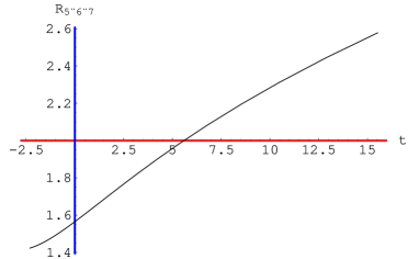
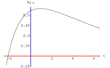
Figure 12: Plots of the scale factors $\overline{r}^{2}_{[\alpha]}$, $\alpha=1|2\,,\,3|4\,,\,5|6|7\,,\,8|9$ as functions of the cosmic time $t=\tau(T)$ with the parameter choice $\omega=0$, $\kappa=3/2$ and for the $A_{2}$ solution with all the roots switched on.

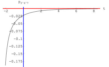
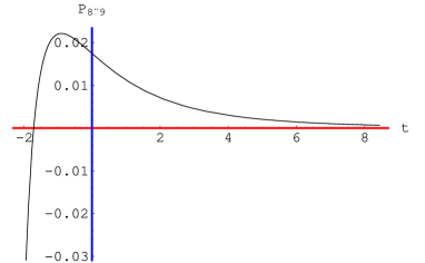
Figure 13: Plots of the pressure eigenvalues $\overline{P}_{[\alpha]}$, $\alpha=1|2\,,\,3|4\,,\,5|6|7\,,\,8|9$ as functions of the cosmic time $t=\tau(T)$ with the parameter choice $\omega=0$, $\kappa=3/2$ and for the $A_{2}$ solution with all the roots switched on.

As already stressed, this a pure $D$-string system and indeed the billiard phenomenon occurs only in the directions 89 that correspond to the euclidean $D$–string world–sheet. In all the other directions there is a monotonous behavior of the scale factors. The $D$-string nature of the solution is best appreciated by looking at the behavior of the pressure eigenvalues, displayed in fig.(13)

As we see the positive bump in the pressure now occurs only in the $D$–string directions 89, while in all the other directions the pressure is the same and rises monotonously to zero from large negative values. The pressure bump is in correspondence with the billiard phenomenon. The energy density is instead a monotonously decreasing function of time (see fig.(14)).

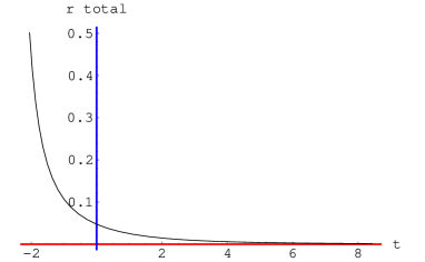
Figure 14: Plot of the energy density as function of the cosmic time $t=\tau(T)$ with the parameter choice $\omega=0$, $\kappa=3/2$ and for the $A_{2}$ solution with all the roots switched on.

An intermediate case is provided by the parameter choice $\omega=1$, $\kappa=0.8<3/2$. The plots of the scale factors are given in fig.(15)

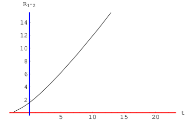
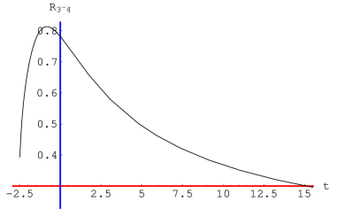
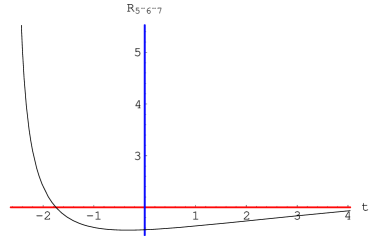
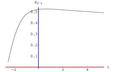
Figure 15: Plots of the scale factors $\overline{r}^{2}_{[\alpha]}$, $\alpha=1|2\,,\,3|4\,,\,5|6|7\,,\,8|9$ as functions of the cosmic time $t=\tau(T)$ with the parameter choice $\omega=1$, $\kappa=0.8$ and for the $A_{2}$ solution with all the roots switched on.

The mixture of $D3$ and $D5$ systems is evident from the pictures. Indeed we have now a billiard phenomenon in both the directions 34 and 89 as we expect from a $D3$–brane, but the maximum in 34 is much sharper than in 89. The maximum in 89 is broader because it takes contribution both from the $D3$ brane and from the $D$–string.

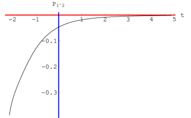
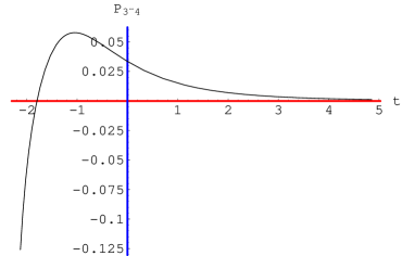
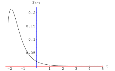
Figure 16: Plots of the pressure eigenvalues $\overline{P}_{[\alpha]}$, $\alpha=1|2\,,\,3|4\,,\,5|6|7\,,\,8|9$ as functions of the cosmic time $t=\tau(T)$ with the parameter choice $\omega=1$, $\kappa=0.8$ and for the $A_{2}$ solution with all the roots switched on.

The phenomenon is best appreciated by considering the plots of the pressure eigenvalues (see figs. (16)) and of the energy density (see figs. (17)). In the pressure plots we see that there is a positive bump both in the directions 34 and 89, yet the bump in 89 is anticipated at earlier times and it is bigger than the bump in 34, the reason being the cooperation between the $D3$–brane and $D$-string contributions. Even more instructive is the plot of the energy densities.

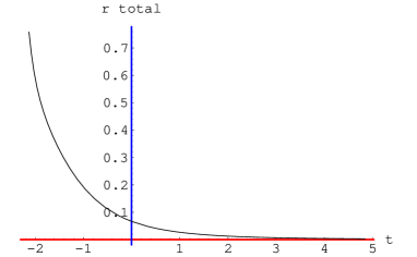
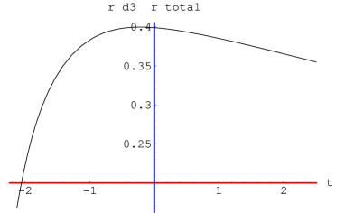
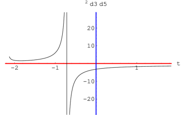
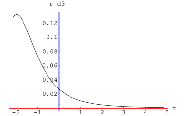
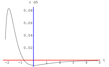
Figure 17: Plots of the energy densities as functions of the cosmic time $t=\tau(T)$ with the parameter choice $\omega=1$, $\kappa=0.8$ and for the $A_{2}$ solution with all the roots switched on. The first picture plots the behaviour of the total energy density. The second plots the ratio of the $D3$–brane contribution to the energy density with respect to the total density. The third plots the ratio of the $D3$–brane contribution with respect to the contribution of the dilaton $D5$–brane system. The fourth and the fifth picture plot the energy density of the $D3$–brane and of the dilaton–$D$–string systems, respectively.

In fig.(17) we see that the energy density of the $D3$–brane has the usual positive bump, while the energy density of the dilaton–$D$–string system has a positive bump followed by a smaller negative one, so that it passes through zero.

At the critical value $\kappa={\textstyle\frac{3}{2}}\omega$ something very interesting occurs in the behaviour of the scale factors.

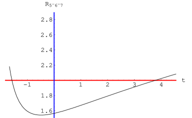
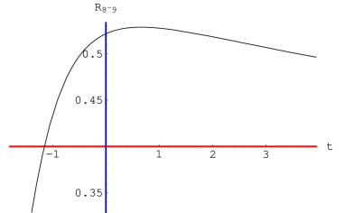
Figure 18: Plots of the scale factors $\overline{r}^{2}_{[\alpha]}$, $\alpha=1|2\,,\,3|4\,,\,5|6|7\,,\,8|9$ as functions of the cosmic time $t=\tau(T)$ with the critical choice of parameters $\omega=1$, $\kappa=3/2$ and for the $A_{2}$ solution with all the roots switched on.

As we see from fig.(18), the scale factor in the direction 34, rather than starting from zero as in all other cases starts from a finite value and then always decreases without suffering a billiard bump. The bump is only in the scale factor 89. Essentially this means that the positive energy of the $D3$ brane and the negative one of the $D$-string exactly compensate at the origin of time for these critical value of the parameters.

5.2.6 Summarizing the above discussion and the cosmological billiard

Summarizing what we have learned from the numerical analysis of the type II B cosmological backgrounds obtained by a specific oxidation of the $A_{2}$ sigma model solutions we can say what follows.

The expansion or contraction of the cosmological scale factors in the diagonal metric is driven by the presence of euclidean $D$–branes which behave like instantons (S-branes). Their energy–density and charge are localized functions of time. Alternatively we see that these branes contribute rather sharp bumps in the eigenvalues of the spatial part of the stress–energy tensor which we have named pressures. Typically there are maxima of these pressures in the space directions parallell to the euclidean brane world–volume and minima of the same in the directions transverse to the brane. These maxima and minima in the pressures correspond to maxima and minima of the scale factors in the same directions. Such inversions in the rate of expansion/contraction of the scale factors is the cosmological billiard phenomenon originally envisaged by Damour et al. In the toy $A_{2}$ model we have presented, we observe just one scattering, but this is due to the insufficient number of branes (roots in the Lie algebra language) that we have excited. Indeed it is like we had only one wall of a Weyl chamber. In subsequent publications we plan to study the phenomenon in more complex situations with more algebraic roots switched on. What is relevant in our opinion is that we were able to see the postulated bumping phenomenon in the context of exact smooth solutions rather than in asymptotic limiting regimes.

6 Conclusions and Perspectives

The main purpose of our analysis was to develop a convenient mathematical framework within three dimensional (ungauged) maximal supergravity where to study homogeneous cosmological solutions of type II A or II B theories. Our approach exploits the correspondence between homogeneous time–dependent solutions in ten and three dimensions. This mapping is realized through toroidal dimensional reduction from $D=10$ to $D=3$ or through oxidation from $D=3$ to $D=10$. The starting point of our study was the ${\rm E}_{8(8)}$ orbit described by three dimensional homogeneous solutions and we defined the precise method for constructing a generic representative of the orbit from the generating solution which is defined only by the radii of the internal seven–torus and the dilaton. Exploiting the solvable Lie algebra (or Iwasawa) representation of the scalar manifold in the three dimensional theory it was possible to control the ten dimensional interpretation of the various bosonic fields. This allows for instance to construct a ten dimensional solution characterized by certain (off–diagonal) components of the metric or of the tensor fields by oxiding a three dimensional solution in which the scalar fields associated with the corresponding ${\rm E}_{8(8)}$ roots are switched on. As an example we have worked out in three dimensions the general homogeneous time–dependent solution of an $A_{2}$ model in which the scalar fields span a ${\rm SL}(3,\mathbb{R})/{\rm SO}(3)$ submanifold of ${\rm E}_{8(8)}/{\rm SO}(16)$. It was shown that, depending on the embedding of ${\rm SL}(3,\mathbb{R})$ within ${\rm E}_{8(8)}$ the ten dimensional solution obtained upon oxidation of the three dimensional one can have radically different physical interpretations in terms of ten dimensional fields. We have then focused on one particular embedding for which the axionic fields are interpreted as the components $B_{34}$, $C_{89}$ and $C_{3489}$ of the type II B tensor fields, and accomplished the oxidation of the solution to ten dimensions. Its behavior, which has been described in detail in the previous section, is characterized by an exchange of energy between the tensor fields and the gravitational field which results in consecutive phases of expansion and contraction of the cosmological scale factors along the directions defined by the non vanishing components of the tensor fields (the “bouncing” behavior of the scale factors in this kind of solutions was also analyzed by Emparan and Arriga in a different perspective [8]). This background could be interpreted microscopically in terms of a system of space–like or S–branes (or SD–branes) [7, 8] along the directions $89$ and $3489$, coupled to the Kalb–Ramond field.

It is interesting to make contact with the cosmological billiard phenomenon describing the behavior of solutions to Einstein equations near space–like singularities. In this limit the evolution of the scale–factors/dilatons is described by a null trajectory in a hyperbolic space which is reflected by walls or hyper–surfaces where the energy density of the axionic fields diverges. Although ours is a different kind of analysis which aims at the construction of exact smooth cosmological solutions, we may retrieve a similar qualitative description of the evolution of the scale–factors/dilaton in relation to the evolution of the axionic fields. In our formalism the logarithm $\sigma_{i}$ of the scale factors associated with the internal directions together with the ten dimensional dilaton $\phi$ are described by the vector $h(t)$ in the Euclidean eight–dimensional space of the ${\rm E}_{8(8)}$ Cartan subalgebra. The kinetic term of an axion $\chi$ associated with the positive ${\rm E}_{8(8)}$ root $\alpha$ contains the characteristic exponential factor $\exp{(-2\,\alpha\cdot h)}$. The corresponding wall in the space of $h$ is defined by the equation $\alpha\cdot h=0$ and the billiard region by $\alpha\cdot h\geq 0$. As it can be inferred from our solution, the evolution of $h(t)$ is such that, if we denote by $h^{\|}$ the component of $h$ along $\alpha$ and by $h^{\perp}$ its projection on the hyperplane perpendicular to $\alpha$ (the wall), as the energy density of $\chi$ reaches its maximum (this temporal region corresponds to the thickness of the S–branes in the $A_{2}$ solution) $h$ undergoes a reflection. This is most easily illustrated for example in the $A_{2}$ solution with just one root switched on (namely $\alpha[80]$). In this case the component of $\dot{h}$ parallel to $\alpha[80]$ undergoes a continuous sign inversion from negative values to positive ones while $|\dot{h}^{\perp}|$ is constant and proportional to the time derivative of the dilaton :

$$\dot{h}^{\|}\rightarrow-\dot{h}^{\|}\,\,\,;\,\,\,|\dot{h}^{\perp}|\,=\,\frac{k}{2\sqrt{6}}\,\propto\,\dot{\phi}\,=\,\mbox{const.}$$ (6.1)

The roots in the $A_{2}$ system are not enough to define a finite volume billiard which would result in an oscillatory behavior of the solution. Indeed, using for $h$ the parametrization in terms of the variables $x,\,y$, namely $h=\{x,x,y,y,y,-y,-y,y\}$, the billiard region is defined by the dominant walls $\alpha[69]\cdot h=0,\,\alpha[15]\cdot h=0$:

$$x \geq 0\,;\,\,\,y\leq-\frac{x}{3}$$ (6.2)

which is an open region. This explains the Kasner–like (non–oscillatory) behavior of our solution for $t\rightarrow+\infty$.

As a possible direction for future investigations, it would be interesting to extend the solution–constructing technology developed in the present paper to one dimensional theories, in which the symmetry group is ${\rm E}_{10(10)}$ [34]–[38] and the Cartan fields $h$ evolve in a ten dimensional Lorentzian space. In this setting a system of axions can be chosen so as to define through their roots a finite billiard, yielding an oscillatory ten dimensional cosmological solution with chaotic behavior.

In perspective it would be also interesting to analyze more general ten dimensional homogeneous solutions deriving from the coupling of gravity to various other combinations of tensor fields and with a non–diagonal metric. We leave for instance to future investigations the construction of backgrounds related to the other classes of $A_{2}$ embeddings outlined in section 5. These backgrounds can provide cosmological settings where to analyze interesting braneworld scenarios, in which the dynamics of the universe expansion/contraction along directions parallel to the braneworld (our four–dimensional universe) and transverse to it would in general be different.

Of course any microscopic interpretation of these homogeneous backgrounds will bring about the issue of $\alpha^{\prime}$ corrections (as far as S–brane supergravity solutions are concerned see [61, 62, 63]) and the possibility of constructing exact string solutions. This is in general not the case for standard cosmological backgrounds, on which stringy corrections have a relevant effect.

An other direction for future research would be to generalize our solution–constructing technique to ansaetze which are inomogeneous/anisotropic with respect to the three–dimensional space–time and to analyze the behavior of these solutions in relation for instance to the singularity theorem discussed in [8].

7 Acknowledgments

M. T. would like to thank M. Bertolini and B. Stefanski for useful discussions.

Appendix A Listing of the $E_{8}$ positive roots

A.1 Listing according to height

In this listing we present the roots of the $E_{8}$ Lie algebra, giving their definition both in terms of the simple roots and in the eucledian basis. The notation $a_{i|j}$ is introduced to denote the height of the root (i). The number (j) is introduced to distinguish the roots of the same height

$$\begin{array}[]{lclclcl}{a_{1|1}}&=&{\alpha[}1]&=&\{1,0,0,0,0,0,0,0\}&=&\{0,1,-1,0,0,0,0,0\}\\ {a_{1|2}}&=&{\alpha[}2]&=&\{0,1,0,0,0,0,0,0\}&=&\{0,0,1,-1,0,0,0,0\}\\ {a_{1|3}}&=&{\alpha[}3]&=&\{0,0,1,0,0,0,0,0\}&=&\{0,0,0,1,-1,0,0,0\}\\ {a_{1|4}}&=&{\alpha[}4]&=&\{0,0,0,1,0,0,0,0\}&=&\{0,0,0,0,1,-1,0,0\}\\ {a_{1|5}}&=&{\alpha[}5]&=&\{0,0,0,0,1,0,0,0\}&=&\{0,0,0,0,0,1,-1,0\}\\ {a_{1|6}}&=&{\alpha[}6]&=&\{0,0,0,0,0,1,0,0\}&=&\{0,0,0,0,0,1,1,0\}\\ {a_{1|7}}&=&{\alpha[}7]&=&\{0,0,0,0,0,0,1,0\}&=&\big{\{}-\frac{1}{2},-\frac{1}{2},-\frac{1}{2},-\frac{1}{2},-\frac{1}{2},-\frac{1}{2},-\frac{1}{2},-\frac{1}{2}\big{\}}\\ {a_{1|8}}&=&{\alpha[}8]&=&\{0,0,0,0,0,0,0,1\}&=&\big{\{}1,-1,0,0,0,0,0,0\big{\}}\\ {a_{2|1}}&=&{\alpha[}9]&=&\{1,1,0,0,0,0,0,0\}&=&\{0,1,0,-1,0,0,0,0\}\\ {a_{2|2}}&=&{\alpha[}10]&=&\{1,0,0,0,0,0,0,1\}&=&\big{\{}1,0,-1,0,0,0,0,0\big{\}}\\ {a_{2|3}}&=&{\alpha[}11]&=&\{0,1,1,0,0,0,0,0\}&=&\{0,0,1,0,-1,0,0,0\}\\ {a_{2|4}}&=&{\alpha[}12]&=&\{0,0,1,1,0,0,0,0\}&=&\{0,0,0,1,0,-1,0,0\}\\ {a_{2|5}}&=&{\alpha[}13]&=&\{0,0,0,1,1,0,0,0\}&=&\{0,0,0,0,1,0,-1,0\}\\ {a_{2|6}}&=&{\alpha[}14]&=&\{0,0,0,1,0,1,0,0\}&=&\{0,0,0,0,1,0,1,0\}\\ {a_{2|7}}&=&{\alpha[}15]&=&\{0,0,0,0,0,1,1,0\}&=&\big{\{}-\frac{1}{2},-\frac{1}{2},-\frac{1}{2},-\frac{1}{2},-\frac{1}{2},\frac{1}{2},\frac{1}{2},-\frac{1}{2}\big{\}}\\ {a_{3|1}}&=&{\alpha[}16]&=&\{1,1,1,0,0,0,0,0\}&=&\{0,1,0,0,-1,0,0,0\}\\ {a_{3|2}}&=&{\alpha[}17]&=&\{1,1,0,0,0,0,0,1\}&=&\big{\{}1,0,0,-1,0,0,0,0\big{\}}\\ {a_{3|3}}&=&{\alpha[}18]&=&\{0,1,1,1,0,0,0,0\}&=&\{0,0,1,0,0,-1,0,0\}\\ {a_{3|4}}&=&{\alpha[}19]&=&\{0,0,1,1,1,0,0,0\}&=&\{0,0,0,1,0,0,-1,0\}\\ {a_{3|5}}&=&{\alpha[}20]&=&\{0,0,1,1,0,1,0,0\}&=&\{0,0,0,1,0,0,1,0\}\\ {a_{3|6}}&=&{\alpha[}21]&=&\{0,0,0,1,0,1,1,0\}&=&\big{\{}-\frac{1}{2},-\frac{1}{2},-\frac{1}{2},-\frac{1}{2},\frac{1}{2},-\frac{1}{2},\frac{1}{2},-\frac{1}{2}\big{\}}\\ {a_{3|7}}&=&{\alpha[}22]&=&\{0,0,0,1,1,1,0,0\}&=&\{0,0,0,0,1,1,0,0\}\\ {a_{4|1}}&=&{\alpha[}23]&=&\{1,1,1,1,0,0,0,0\}&=&\{0,1,0,0,0,-1,0,0\}\\ {a_{4|2}}&=&{\alpha[}24]&=&\{0,1,1,1,1,0,0,0\}&=&\{0,0,1,0,0,0,-1,0\}\\ {a_{4|3}}&=&{\alpha[}25]&=&\{0,1,1,1,0,1,0,0\}&=&\{0,0,1,0,0,0,1,0\}\\ {a_{4|4}}&=&{\alpha[}26]&=&\{1,1,1,0,0,0,0,1\}&=&\big{\{}1,0,0,0,-1,0,0,0\big{\}}\\ {a_{4|5}}&=&{\alpha[}27]&=&\{0,0,1,1,0,1,1,0\}&=&\big{\{}-\frac{1}{2},-\frac{1}{2},-\frac{1}{2},\frac{1}{2},-\frac{1}{2},-\frac{1}{2},\frac{1}{2},-\frac{1}{2}\big{\}}\\ {a_{4|6}}&=&{\alpha[}28]&=&\{0,0,1,1,1,1,0,0\}&=&\{0,0,0,1,0,1,0,0\}\end{array}$$

$$\begin{array}[]{lclclcl}{a_{4|7}}&=&{\alpha[}29]&=&\{0,0,0,1,1,1,1,0\}&=&\big{\{}-\frac{1}{2},-\frac{1}{2},-\frac{1}{2},-\frac{1}{2},\frac{1}{2},\frac{1}{2},-\frac{1}{2},-\frac{1}{2}\big{\}}\\ {a_{5|1}}&=&{\alpha[}30]&=&\{1,1,1,1,1,0,0,0\}&=&\{0,1,0,0,0,0,-1,0\}\\ {a_{5|2}}&=&{\alpha[}31]&=&\{1,1,1,1,0,1,0,0\}&=&\{0,1,0,0,0,0,1,0\}\\ {a_{5|3}}&=&{\alpha[}32]&=&\{0,1,1,1,0,1,1,0\}&=&\big{\{}-\frac{1}{2},-\frac{1}{2},\frac{1}{2},-\frac{1}{2},-\frac{1}{2},-\frac{1}{2},\frac{1}{2},-\frac{1}{2}\big{\}}\\ {a_{5|4}}&=&{\alpha[}33]&=&\{0,1,1,1,1,1,0,0\}&=&\{0,0,1,0,0,1,0,0\}\\ {a_{5|5}}&=&{\alpha[}34]&=&\{0,0,1,1,1,1,1,0\}&=&\big{\{}-\frac{1}{2},-\frac{1}{2},-\frac{1}{2},\frac{1}{2},-\frac{1}{2},\frac{1}{2},-\frac{1}{2},-\frac{1}{2}\big{\}}\\ {a_{5|6}}&=&{\alpha[}35]&=&\{1,1,1,1,0,0,0,1\}&=&\big{\{}1,0,0,0,0,-1,0,0\big{\}}\\ {a_{5|7}}&=&{\alpha[}36]&=&\{0,0,1,2,1,1,0,0\}&=&\{0,0,0,1,1,0,0,0\}\\ {a_{6|1}}&=&{\alpha[}37]&=&\{1,1,1,1,0,1,1,0\}&=&\big{\{}-\frac{1}{2},\frac{1}{2},-\frac{1}{2},-\frac{1}{2},-\frac{1}{2},-\frac{1}{2},\frac{1}{2},-\frac{1}{2}\big{\}}\\ {a_{6|2}}&=&{\alpha[}38]&=&\{1,1,1,1,1,1,0,0\}&=&\{0,1,0,0,0,1,0,0\}\\ {a_{6|3}}&=&{\alpha[}39]&=&\{0,1,1,1,1,1,1,0\}&=&\big{\{}-\frac{1}{2},-\frac{1}{2},\frac{1}{2},-\frac{1}{2},-\frac{1}{2},\frac{1}{2},-\frac{1}{2},-\frac{1}{2}\big{\}}\\ {a_{6|4}}&=&{\alpha[}40]&=&\{0,1,1,2,1,1,0,0\}&=&\{0,0,1,0,1,0,0,0\}\\ {a_{6|5}}&=&{\alpha[}41]&=&\{0,0,1,2,1,1,1,0\}&=&\big{\{}-\frac{1}{2},-\frac{1}{2},-\frac{1}{2},\frac{1}{2},\frac{1}{2},-\frac{1}{2},-\frac{1}{2},-\frac{1}{2}\big{\}}\\ {a_{6|6}}&=&{\alpha[}42]&=&\{1,1,1,1,1,0,0,1\}&=&\big{\{}1,0,0,0,0,0,-1,0\big{\}}\\ {a_{6|7}}&=&{\alpha[}43]&=&\{1,1,1,1,0,1,0,1\}&=&\big{\{}1,0,0,0,0,0,1,0\big{\}}\\ {a_{7|1}}&=&{\alpha[}44]&=&\{1,1,1,1,1,1,1,0\}&=&\big{\{}-\frac{1}{2},\frac{1}{2},-\frac{1}{2},-\frac{1}{2},-\frac{1}{2},\frac{1}{2},-\frac{1}{2},-\frac{1}{2}\big{\}}\\ {a_{7|2}}&=&{\alpha[}45]&=&\{1,1,1,2,1,1,0,0\}&=&\{0,1,0,0,1,0,0,0\}\\ {a_{7|3}}&=&{\alpha[}46]&=&\{0,1,1,2,1,1,1,0\}&=&\big{\{}-\frac{1}{2},-\frac{1}{2},\frac{1}{2},-\frac{1}{2},\frac{1}{2},-\frac{1}{2},-\frac{1}{2},-\frac{1}{2}\big{\}}\\ {a_{7|4}}&=&{\alpha[}47]&=&\{0,1,2,2,1,1,0,0\}&=&\{0,0,1,1,0,0,0,0\}\\ {a_{7|5}}&=&{\alpha[}48]&=&\{1,1,1,1,1,1,0,1\}&=&\big{\{}1,0,0,0,0,1,0,0\big{\}}\\ {a_{7|6}}&=&{\alpha[}49]&=&\{0,0,1,2,1,2,1,0\}&=&\big{\{}-\frac{1}{2},-\frac{1}{2},-\frac{1}{2},\frac{1}{2},\frac{1}{2},\frac{1}{2},\frac{1}{2},-\frac{1}{2}\big{\}}\\ {a_{7|7}}&=&{\alpha[}50]&=&\{1,1,1,1,0,1,1,1\}&=&\big{\{}\frac{1}{2},-\frac{1}{2},-\frac{1}{2},-\frac{1}{2},-\frac{1}{2},-\frac{1}{2},\frac{1}{2},-\frac{1}{2}\big{\}}\\ {a_{8|1}}&=&{\alpha[}51]&=&\{1,1,1,2,1,1,1,0\}&=&\big{\{}-\frac{1}{2},\frac{1}{2},-\frac{1}{2},-\frac{1}{2},\frac{1}{2},-\frac{1}{2},-\frac{1}{2},-\frac{1}{2}\big{\}}\\ {a_{8|2}}&=&{\alpha[}52]&=&\{1,1,2,2,1,1,0,0\}&=&\{0,1,0,1,0,0,0,0\}\\ {a_{8|3}}&=&{\alpha[}53]&=&\{0,1,1,2,1,2,1,0\}&=&\big{\{}-\frac{1}{2},-\frac{1}{2},\frac{1}{2},-\frac{1}{2},\frac{1}{2},\frac{1}{2},\frac{1}{2},-\frac{1}{2}\big{\}}\\ {a_{8|4}}&=&{\alpha[}54]&=&\{0,1,2,2,1,1,1,0\}&=&\big{\{}-\frac{1}{2},-\frac{1}{2},\frac{1}{2},\frac{1}{2},-\frac{1}{2},-\frac{1}{2},-\frac{1}{2},-\frac{1}{2}\big{\}}\\ {a_{8|5}}&=&{\alpha[}55]&=&\{1,1,1,2,1,1,0,1\}&=&\big{\{}1,0,0,0,1,0,0,0\big{\}}\\ {a_{8|6}}&=&{\alpha[}56]&=&\{1,1,1,1,1,1,1,1\}&=&\big{\{}\frac{1}{2},-\frac{1}{2},-\frac{1}{2},-\frac{1}{2},-\frac{1}{2},\frac{1}{2},-\frac{1}{2},-\frac{1}{2}\big{\}}\\ {a_{9|1}}&=&{\alpha[}57]&=&\{1,1,1,2,1,2,1,0\}&=&\big{\{}-\frac{1}{2},\frac{1}{2},-\frac{1}{2},-\frac{1}{2},\frac{1}{2},\frac{1}{2},\frac{1}{2},-\frac{1}{2}\big{\}}\\ {a_{9|2}}&=&{\alpha[}58]&=&\{1,1,2,2,1,1,1,0\}&=&\big{\{}-\frac{1}{2},\frac{1}{2},-\frac{1}{2},\frac{1}{2},-\frac{1}{2},-\frac{1}{2},-\frac{1}{2},-\frac{1}{2}\big{\}}\\ {a_{9|3}}&=&{\alpha[}59]&=&\{1,2,2,2,1,1,0,0\}&=&\{0,1,1,0,0,0,0,0\}\\ {a_{9|4}}&=&{\alpha[}60]&=&\{0,1,2,2,1,2,1,0\}&=&\big{\{}-\frac{1}{2},-\frac{1}{2},\frac{1}{2},\frac{1}{2},-\frac{1}{2},\frac{1}{2},\frac{1}{2},-\frac{1}{2}\big{\}}\\ {a_{9|5}}&=&{\alpha[}61]&=&\{1,1,2,2,1,1,0,1\}&=&\big{\{}1,0,0,1,0,0,0,0\big{\}}\\ {a_{9|6}}&=&{\alpha[}62]&=&\{1,1,1,2,1,1,1,1\}&=&\big{\{}\frac{1}{2},-\frac{1}{2},-\frac{1}{2},-\frac{1}{2},\frac{1}{2},-\frac{1}{2},-\frac{1}{2},-\frac{1}{2}\big{\}}\end{array}$$

$$\begin{array}[]{lclclcl}{a_{10|1}}&=&{\alpha[}63]&=&\{1,1,2,2,1,2,1,0\}&=&\big{\{}-\frac{1}{2},\frac{1}{2},-\frac{1}{2},\frac{1}{2},-\frac{1}{2},\frac{1}{2},\frac{1}{2},-\frac{1}{2}\big{\}}\\ {a_{10|2}}&=&{\alpha[}64]&=&\{1,2,2,2,1,1,1,0\}&=&\big{\{}-\frac{1}{2},\frac{1}{2},\frac{1}{2},-\frac{1}{2},-\frac{1}{2},-\frac{1}{2},-\frac{1}{2},-\frac{1}{2}\big{\}}\\ {a_{10|3}}&=&{\alpha[}65]&=&\{1,2,2,2,1,1,0,1\}&=&\big{\{}1,0,1,0,0,0,0,0\big{\}}\\ {a_{10|4}}&=&{\alpha[}66]&=&\{1,1,2,2,1,1,1,1\}&=&\big{\{}\frac{1}{2},-\frac{1}{2},-\frac{1}{2},\frac{1}{2},-\frac{1}{2},-\frac{1}{2},-\frac{1}{2},-\frac{1}{2}\big{\}}\\ {a_{10|5}}&=&{\alpha[}67]&=&\{0,1,2,3,1,2,1,0\}&=&\big{\{}-\frac{1}{2},-\frac{1}{2},\frac{1}{2},\frac{1}{2},\frac{1}{2},-\frac{1}{2},\frac{1}{2},-\frac{1}{2}\big{\}}\\ {a_{10|6}}&=&{\alpha[}68]&=&\{1,1,1,2,1,2,1,1\}&=&\big{\{}\frac{1}{2},-\frac{1}{2},-\frac{1}{2},-\frac{1}{2},\frac{1}{2},\frac{1}{2},\frac{1}{2},-\frac{1}{2}\big{\}}\\ {a_{11|1}}&=&{\alpha[}69]&=&\{2,2,2,2,1,1,0,1\}&=&\big{\{}1,1,0,0,0,0,0,0\big{\}}\\ {a_{11|2}}&=&{\alpha[}70]&=&\{1,1,2,3,1,2,1,0\}&=&\big{\{}-\frac{1}{2},\frac{1}{2},-\frac{1}{2},\frac{1}{2},\frac{1}{2},-\frac{1}{2},\frac{1}{2},-\frac{1}{2}\big{\}}\\ {a_{11|3}}&=&{\alpha[}71]&=&\{1,2,2,2,1,2,1,0\}&=&\big{\{}-\frac{1}{2},\frac{1}{2},\frac{1}{2},-\frac{1}{2},-\frac{1}{2},\frac{1}{2},\frac{1}{2},-\frac{1}{2}\big{\}}\\ {a_{11|4}}&=&{\alpha[}72]&=&\{1,2,2,2,1,1,1,1\}&=&\big{\{}\frac{1}{2},-\frac{1}{2},\frac{1}{2},-\frac{1}{2},-\frac{1}{2},-\frac{1}{2},-\frac{1}{2},-\frac{1}{2}\big{\}}\\ {a_{11|5}}&=&{\alpha[}73]&=&\{1,1,2,2,1,2,1,1\}&=&\big{\{}\frac{1}{2},-\frac{1}{2},-\frac{1}{2},\frac{1}{2},-\frac{1}{2},\frac{1}{2},\frac{1}{2},-\frac{1}{2}\big{\}}\\ {a_{11|6}}&=&{\alpha[}74]&=&\{0,1,2,3,2,2,1,0\}&=&\big{\{}-\frac{1}{2},-\frac{1}{2},\frac{1}{2},\frac{1}{2},\frac{1}{2},\frac{1}{2},-\frac{1}{2},-\frac{1}{2}\big{\}}\\ {a_{12|1}}&=&{\alpha[}75]&=&\{2,2,2,2,1,1,1,1\}&=&\big{\{}\frac{1}{2},\frac{1}{2},-\frac{1}{2},-\frac{1}{2},-\frac{1}{2},-\frac{1}{2},-\frac{1}{2},-\frac{1}{2}\big{\}}\\ {a_{12|2}}&=&{\alpha[}76]&=&\{1,1,2,3,2,2,1,0\}&=&\big{\{}-\frac{1}{2},\frac{1}{2},-\frac{1}{2},\frac{1}{2},\frac{1}{2},\frac{1}{2},-\frac{1}{2},-\frac{1}{2}\big{\}}\\ {a_{12|3}}&=&{\alpha[}77]&=&\{1,2,2,3,1,2,1,0\}&=&\big{\{}-\frac{1}{2},\frac{1}{2},\frac{1}{2},-\frac{1}{2},\frac{1}{2},-\frac{1}{2},\frac{1}{2},-\frac{1}{2}\big{\}}\\ {a_{12|4}}&=&{\alpha[}78]&=&\{1,2,2,2,1,2,1,1\}&=&\big{\{}\frac{1}{2},-\frac{1}{2},\frac{1}{2},-\frac{1}{2},-\frac{1}{2},\frac{1}{2},\frac{1}{2},-\frac{1}{2}\big{\}}\\ {a_{12|5}}&=&{\alpha[}79]&=&\{1,1,2,3,1,2,1,1\}&=&\big{\{}\frac{1}{2},-\frac{1}{2},-\frac{1}{2},\frac{1}{2},\frac{1}{2},-\frac{1}{2},\frac{1}{2},-\frac{1}{2}\big{\}}\\ {a_{13|1}}&=&{\alpha[}80]&=&\{2,2,2,2,1,2,1,1\}&=&\big{\{}\frac{1}{2},\frac{1}{2},-\frac{1}{2},-\frac{1}{2},-\frac{1}{2},\frac{1}{2},\frac{1}{2},-\frac{1}{2}\big{\}}\\ {a_{13|2}}&=&{\alpha[}81]&=&\{1,2,2,3,2,2,1,0\}&=&\big{\{}-\frac{1}{2},\frac{1}{2},\frac{1}{2},-\frac{1}{2},\frac{1}{2},\frac{1}{2},-\frac{1}{2},-\frac{1}{2}\big{\}}\\ {a_{13|3}}&=&{\alpha[}82]&=&\{1,2,2,3,1,2,1,1\}&=&\big{\{}\frac{1}{2},-\frac{1}{2},\frac{1}{2},-\frac{1}{2},\frac{1}{2},-\frac{1}{2},\frac{1}{2},-\frac{1}{2}\big{\}}\\ {a_{13|4}}&=&{\alpha[}83]&=&\{1,2,3,3,1,2,1,0\}&=&\big{\{}-\frac{1}{2},\frac{1}{2},\frac{1}{2},\frac{1}{2},-\frac{1}{2},-\frac{1}{2},\frac{1}{2},-\frac{1}{2}\big{\}}\\ {a_{13|5}}&=&{\alpha[}84]&=&\{1,1,2,3,2,2,1,1\}&=&\big{\{}\frac{1}{2},-\frac{1}{2},-\frac{1}{2},\frac{1}{2},\frac{1}{2},\frac{1}{2},-\frac{1}{2},-\frac{1}{2}\big{\}}\\ {a_{14|1}}&=&{\alpha[}85]&=&\{2,2,2,3,1,2,1,1\}&=&\big{\{}\frac{1}{2},\frac{1}{2},-\frac{1}{2},-\frac{1}{2},\frac{1}{2},-\frac{1}{2},\frac{1}{2},-\frac{1}{2}\big{\}}\\ {a_{14|2}}&=&{\alpha[}86]&=&\{1,2,2,3,2,2,1,1\}&=&\big{\{}\frac{1}{2},-\frac{1}{2},\frac{1}{2},-\frac{1}{2},\frac{1}{2},\frac{1}{2},-\frac{1}{2},-\frac{1}{2}\big{\}}\\ {a_{14|3}}&=&{\alpha[}87]&=&\{1,2,3,3,2,2,1,0\}&=&\big{\{}-\frac{1}{2},\frac{1}{2},\frac{1}{2},\frac{1}{2},-\frac{1}{2},\frac{1}{2},-\frac{1}{2},-\frac{1}{2}\big{\}}\\ {a_{14|4}}&=&{\alpha[}88]&=&\{1,2,3,3,1,2,1,1\}&=&\big{\{}\frac{1}{2},-\frac{1}{2},\frac{1}{2},\frac{1}{2},-\frac{1}{2},-\frac{1}{2},\frac{1}{2},-\frac{1}{2}\big{\}}\\ {a_{15|1}}&=&{\alpha[}89]&=&\{2,2,2,3,2,2,1,1\}&=&\big{\{}\frac{1}{2},\frac{1}{2},-\frac{1}{2},-\frac{1}{2},\frac{1}{2},\frac{1}{2},-\frac{1}{2},-\frac{1}{2}\big{\}}\\ {a_{15|2}}&=&{\alpha[}90]&=&\{2,2,3,3,1,2,1,1\}&=&\big{\{}\frac{1}{2},\frac{1}{2},-\frac{1}{2},\frac{1}{2},-\frac{1}{2},-\frac{1}{2},\frac{1}{2},-\frac{1}{2}\big{\}}\\ {a_{15|3}}&=&{\alpha[}91]&=&\{1,2,3,3,2,2,1,1\}&=&\big{\{}\frac{1}{2},-\frac{1}{2},\frac{1}{2},\frac{1}{2},-\frac{1}{2},\frac{1}{2},-\frac{1}{2},-\frac{1}{2}\big{\}}\\ {a_{15|4}}&=&{\alpha[}92]&=&\{1,2,3,4,2,2,1,0\}&=&\big{\{}-\frac{1}{2},\frac{1}{2},\frac{1}{2},\frac{1}{2},\frac{1}{2},-\frac{1}{2},-\frac{1}{2},-\frac{1}{2}\big{\}}\\ {a_{16|1}}&=&{\alpha[}93]&=&\{2,2,3,3,2,2,1,1\}&=&\big{\{}\frac{1}{2},\frac{1}{2},-\frac{1}{2},\frac{1}{2},-\frac{1}{2},\frac{1}{2},-\frac{1}{2},-\frac{1}{2}\big{\}}\\ {a_{16|2}}&=&{\alpha[}94]&=&\{2,3,3,3,1,2,1,1\}&=&\big{\{}\frac{1}{2},\frac{1}{2},\frac{1}{2},-\frac{1}{2},-\frac{1}{2},-\frac{1}{2},\frac{1}{2},-\frac{1}{2}\big{\}}\\ {a_{16|3}}&=&{\alpha[}95]&=&\{1,2,3,4,2,2,1,1\}&=&\big{\{}\frac{1}{2},-\frac{1}{2},\frac{1}{2},\frac{1}{2},\frac{1}{2},-\frac{1}{2},-\frac{1}{2},-\frac{1}{2}\big{\}}\\ {a_{16|4}}&=&{\alpha[}96]&=&\{1,2,3,4,2,3,1,0\}&=&\big{\{}-\frac{1}{2},\frac{1}{2},\frac{1}{2},\frac{1}{2},\frac{1}{2},\frac{1}{2},\frac{1}{2},-\frac{1}{2}\big{\}}\end{array}$$

$$\begin{array}[]{lclclcl}{a_{17|1}}&=&{\alpha[}97]&=&\{2,2,3,4,2,2,1,1\}&=&\big{\{}\frac{1}{2},\frac{1}{2},-\frac{1}{2},\frac{1}{2},\frac{1}{2},-\frac{1}{2},-\frac{1}{2},-\frac{1}{2}\big{\}}\\ {a_{17|2}}&=&{\alpha[}98]&=&\{2,3,3,3,2,2,1,1\}&=&\big{\{}\frac{1}{2},\frac{1}{2},\frac{1}{2},-\frac{1}{2},-\frac{1}{2},\frac{1}{2},-\frac{1}{2},-\frac{1}{2}\big{\}}\\ {a_{17|3}}&=&{\alpha[}99]&=&\{1,2,3,4,2,3,1,1\}&=&\big{\{}\frac{1}{2},-\frac{1}{2},\frac{1}{2},\frac{1}{2},\frac{1}{2},\frac{1}{2},\frac{1}{2},-\frac{1}{2}\big{\}}\\ {a_{17|4}}&=&{\alpha[}100]&=&\{1,2,3,4,2,3,2,0\}&=&\big{\{}-1,0,0,0,0,0,0,-1\big{\}}\\ {a_{18|1}}&=&{\alpha[}101]&=&\{2,2,3,4,2,3,1,1\}&=&\big{\{}\frac{1}{2},\frac{1}{2},-\frac{1}{2},\frac{1}{2},\frac{1}{2},\frac{1}{2},\frac{1}{2},-\frac{1}{2}\big{\}}\\ {a_{18|2}}&=&{\alpha[}102]&=&\{2,3,3,4,2,2,1,1\}&=&\big{\{}\frac{1}{2},\frac{1}{2},\frac{1}{2},-\frac{1}{2},\frac{1}{2},-\frac{1}{2},-\frac{1}{2},-\frac{1}{2}\big{\}}\\ {a_{18|3}}&=&{\alpha[}103]&=&\{1,2,3,4,2,3,2,1\}&=&\big{\{}0,-1,0,0,0,0,0,-1\big{\}}\\ {a_{19|1}}&=&{\alpha[}104]&=&\{2,2,3,4,2,3,2,1\}&=&\big{\{}0,0,-1,0,0,0,0,-1\big{\}}\\ {a_{19|2}}&=&{\alpha[}105]&=&\{2,3,3,4,2,3,1,1\}&=&\big{\{}\frac{1}{2},\frac{1}{2},\frac{1}{2},-\frac{1}{2},\frac{1}{2},\frac{1}{2},\frac{1}{2},-\frac{1}{2}\big{\}}\\ {a_{19|3}}&=&{\alpha[}106]&=&\{2,3,4,4,2,2,1,1\}&=&\big{\{}\frac{1}{2},\frac{1}{2},\frac{1}{2},\frac{1}{2},-\frac{1}{2},-\frac{1}{2},-\frac{1}{2},-\frac{1}{2}\big{\}}\\ {a_{20|1}}&=&{\alpha[}107]&=&\{2,3,3,4,2,3,2,1\}&=&\big{\{}0,0,0,-1,0,0,0,-1\big{\}}\\ {a_{20|2}}&=&{\alpha[}108]&=&\{2,3,4,4,2,3,1,1\}&=&\big{\{}\frac{1}{2},\frac{1}{2},\frac{1}{2},\frac{1}{2},-\frac{1}{2},\frac{1}{2},\frac{1}{2},-\frac{1}{2}\big{\}}\\ {a_{21|1}}&=&{\alpha[}109]&=&\{2,3,4,4,2,3,2,1\}&=&\big{\{}0,0,0,0,-1,0,0,-1\big{\}}\\ {a_{21|2}}&=&{\alpha[}110]&=&\{2,3,4,5,2,3,1,1\}&=&\big{\{}\frac{1}{2},\frac{1}{2},\frac{1}{2},\frac{1}{2},\frac{1}{2},-\frac{1}{2},\frac{1}{2},-\frac{1}{2}\big{\}}\\ {a_{22|1}}&=&{\alpha[}111]&=&\{2,3,4,5,2,3,2,1\}&=&\big{\{}0,0,0,0,0,-1,0,-1\big{\}}\\ {a_{22|2}}&=&{\alpha[}112]&=&\{2,3,4,5,3,3,1,1\}&=&\big{\{}\frac{1}{2},\frac{1}{2},\frac{1}{2},\frac{1}{2},\frac{1}{2},\frac{1}{2},-\frac{1}{2},-\frac{1}{2}\big{\}}\\ {a_{23|1}}&=&{\alpha[}113]&=&\{2,3,4,5,3,3,2,1\}&=&\big{\{}0,0,0,0,0,0,-1,-1\}\\ {a_{23|2}}&=&{\alpha[}114]&=&\{2,3,4,5,2,4,2,1\}&=&\big{\{}0,0,0,0,0,0,1,-1\big{\}}\\ {a_{24|1}}&=&{\alpha[}115]&=&\{2,3,4,5,3,4,2,1\}&=&\big{\{}0,0,0,0,0,1,0,-1\big{\}}\\ {a_{25|1}}&=&{\alpha[}116]&=&\{2,3,4,6,3,4,2,1\}&=&\big{\{}0,0,0,0,1,0,0,-1\big{\}}\\ {a_{26|1}}&=&{\alpha[}117]&=&\{2,3,5,6,3,4,2,1\}&=&\big{\{}0,0,0,1,0,0,0,-1\big{\}}\\ {a_{27|1}}&=&{\alpha[}118]&=&\{2,4,5,6,3,4,2,1\}&=&\big{\{}0,0,1,0,0,0,0,-1\big{\}}\\ {a_{28|1}}&=&{\alpha[}119]&=&\{3,4,5,6,3,4,2,1\}&=&\big{\{}0,1,0,0,0,0,0,-1\big{\}}\\ {a_{29|1}}&=&{\alpha[}120]&=&\{3,4,5,6,3,4,2,2\}&=&\big{\{}1,0,0,0,0,0,0,-1\big{\}}\end{array}$$

A.2 Listing the roots according to the dimensional filtration

Roots in D[ 1 ] and D[ 2 ]

$$\begin{array}[]{lcccl|cc}\hline\cr\mbox{label}&\hbox{}\hfil&\mbox{root number}&\hbox{}\hfil&\mbox{Dynkin label}&\mbox{type II B }&\mbox{type II A }\\ \hline\cr{d_{1|1}}&=&{\alpha[}7]&=&\{0,0,0,0,0,0,1,0\}&\rho&C_{9}\\ {d_{2|1}}&=&{\alpha[}6]&=&\{0,0,0,0,0,1,0,0\}&B_{8\,9}&\gamma_{8}^{\phantom{8}\,9}\\ {d_{2|2}}&=&{\alpha[}5]&=&\{0,0,0,0,1,0,0,0\}&\gamma_{8}{}^{9}&\gamma_{8}{}^{9}\\ {d_{2|3}}&=&{\alpha[}15]&=&\{0,0,0,0,0,1,1,0\}&C_{8\,9}&C_{8}\\ \end{array}$$

Roots in D[ 3 ], D[ 4 ] and D[ 5 ]

$$\begin{array}[]{lcccl|cc}\hline\cr\mbox{label}&\hbox{}\hfil&\mbox{root number}&\hbox{}\hfil&\mbox{Dynkin label}&\mbox{type II B }&\mbox{type II A }\\ \hline\cr{d_{3|1}}&=&{\alpha[}22]&=&\{0,0,0,1,1,1,0,0\}&B_{7\,8}&\gamma_{7}^{\phantom{7}\,8}\\ {d_{3|2}}&=&{\alpha[}4]&=&\{0,0,0,1,0,0,0,0\}&\gamma_{7}{}^{8}&\gamma_{7}{}^{8}\\ {d_{3|3}}&=&{\alpha[}14]&=&\{0,0,0,1,0,1,0,0\}&B_{7\,9}&\gamma_{7}{}^{9}\\ {d_{3|4}}&=&{\alpha[}13]&=&\{0,0,0,1,1,0,0,0\}&\gamma_{7}{}^{9}&B_{7\,9}\\ {d_{3|5}}&=&{\alpha[}29]&=&\{0,0,0,1,1,1,1,0\}&C_{7\,8}&C_{7\,8\,9}\\ {d_{3|6}}&=&{\alpha[}21]&=&\{0,0,0,1,0,1,1,0\}&C_{7\,9}&C_{7}\\ {d_{4|1}}&=&{\alpha[}36]&=&\{0,0,1,2,1,1,0,0\}&B_{6\,7}&B_{6\,7}\\ {d_{4|2}}&=&{\alpha[}3]&=&\{0,0,1,0,0,0,0,0\}&\gamma_{6}{}^{7}&\gamma_{6}{}^{7}\\ {d_{4|3}}&=&{\alpha[}28]&=&\{0,0,1,1,1,1,0,0\}&B_{6\,8}&B_{6\,8}\\ {d_{4|4}}&=&{\alpha[}12]&=&\{0,0,1,1,0,0,0,0\}&\gamma_{6}{}^{8}&\gamma_{6}{}^{8}\\ {d_{4|5}}&=&{\alpha[}20]&=&\{0,0,1,1,0,1,0,0\}&B_{6\,9}&\gamma_{6}{}^{9}\\ {d_{4|6}}&=&{\alpha[}19]&=&\{0,0,1,1,1,0,0,0\}&\gamma_{6}{}^{9}&B_{6\,9}\\ {d_{4|7}}&=&{\alpha[}41]&=&\{0,0,1,2,1,1,1,0\}&C_{6\,7}&C_{6\,7\,9}\\ {d_{4|8}}&=&{\alpha[}34]&=&\{0,0,1,1,1,1,1,0\}&C_{6\,8}&C_{6\,8\,9}\\ {d_{4|9}}&=&{\alpha[}27]&=&\{0,0,1,1,0,1,1,0\}&C_{6\,9}&C_{6}\\ {d_{4|10}}&=&{\alpha[}49]&=&\{0,0,1,2,1,2,1,0\}&C_{6\,7\,8\,9}&C_{6\,7\,8}\\ {d_{5|1}}&=&{\alpha[}47]&=&\{0,1,2,2,1,1,0,0\}&B_{5\,6}&B_{5\,6}\\ {d_{5|2}}&=&{\alpha[}2]&=&\{0,1,0,0,0,0,0,0\}&\gamma_{5}{}^{6}&\gamma_{5}{}^{6}\\ {d_{5|3}}&=&{\alpha[}40]&=&\{0,1,1,2,1,1,0,0\}&B_{5\,7}&B_{5\,7}\\ {d_{5|4}}&=&{\alpha[}11]&=&\{0,1,1,0,0,0,0,0\}&\gamma_{5}{}^{7}&\gamma_{5}{}^{7}\\ {d_{5|5}}&=&{\alpha[}33]&=&\{0,1,1,1,1,1,0,0\}&B_{5\,8}&B_{5\,8}\\ {d_{5|6}}&=&{\alpha[}18]&=&\{0,1,1,1,0,0,0,0\}&\gamma_{5}{}^{8}&\gamma_{5}{}^{8}\\ {d_{5|7}}&=&{\alpha[}25]&=&\{0,1,1,1,0,1,0,0\}&B_{5\,9}&\gamma_{5}{}^{9}\\ {d_{5|8}}&=&{\alpha[}24]&=&\{0,1,1,1,1,0,0,0\}&\gamma_{5}{}^{9}&B_{5\,9}\\ {d_{5|9}}&=&{\alpha[}54]&=&\{0,1,2,2,1,1,1,0\}&C_{5\,6}&C_{5\,6\,9}\\ {d_{5|10}}&=&{\alpha[}46]&=&\{0,1,1,2,1,1,1,0\}&C_{5\,7}&C_{5\,7\,9}\\ {d_{5|11}}&=&{\alpha[}39]&=&\{0,1,1,1,1,1,1,0\}&C_{5\,8}&C_{5\,8\,9}\\ {d_{5|12}}&=&{\alpha[}32]&=&\{0,1,1,1,0,1,1,0\}&C_{5\,9}&C_{5}\\ {d_{5|13}}&=&{\alpha[}53]&=&\{0,1,1,2,1,2,1,0\}&C_{5\,7\,8\,9}&C_{5\,7\,8}\\ {d_{5|14}}&=&{\alpha[}60]&=&\{0,1,2,2,1,2,1,0\}&C_{5\,6\,8\,9}&C_{5\,6\,8}\\ {d_{5|15}}&=&{\alpha[}67]&=&\{0,1,2,3,1,2,1,0\}&C_{5\,6\,7\,9}&C_{5\,6\,7}\\ {d_{5|16}}&=&{\alpha[}74]&=&\{0,1,2,3,2,2,1,0\}&C_{5\,6\,7\,8}&C_{3\,4\,\mu}\\ \end{array}$$

Roots in D[ 6 ]

$$\begin{array}[]{lcccl|cc}\hline\cr\mbox{label}&\hbox{}\hfil&\mbox{root number}&\hbox{}\hfil&\mbox{Dynkin label}&\mbox{type II B }&\mbox{type II A }\\ \hline\cr{d_{6|1}}&=&{\alpha[}59]&=&\{1,2,2,2,1,1,0,0\}&B_{4\,5}&B_{4\,5}\\ {d_{6|2}}&=&{\alpha[}1]&=&\{1,0,0,0,0,0,0,0\}&\gamma_{4}{}^{5}&\gamma_{4}{}^{5}\\ {d_{6|3}}&=&{\alpha[}52]&=&\{1,1,2,2,1,1,0,0\}&B_{4\,6}&B_{4\,6}\\ {d_{6|4}}&=&{\alpha[}9]&=&\{1,1,0,0,0,0,0,0\}&\gamma_{4}{}^{6}&\gamma_{4}{}^{6}\\ {d_{6|5}}&=&{\alpha[}45]&=&\{1,1,1,2,1,1,0,0\}&B_{4\,7}&B_{4\,7}\\ {d_{6|6}}&=&{\alpha[}16]&=&\{1,1,1,0,0,0,0,0\}&\gamma_{4}{}^{7}&\gamma_{4}{}^{7}\\ \ {d_{6|7}}&=&{\alpha[}38]&=&\{1,1,1,1,1,1,0,0\}&B_{4\,8}&B_{4\,8}\\ {d_{6|8}}&=&{\alpha[}23]&=&\{1,1,1,1,0,0,0,0\}&\gamma_{4}{}^{8}&\gamma_{4}{}^{8}\\ {d_{6|9}}&=&{\alpha[}31]&=&\{1,1,1,1,0,1,0,0\}&B_{4\,9}&\gamma_{4}{}^{9}\\ {d_{6|10}}&=&{\alpha[}30]&=&\{1,1,1,1,1,0,0,0\}&\gamma_{4}{}^{9}&B_{4\,9}\\ {d_{6|11}}&=&{\alpha[}100]&=&\{1,2,3,4,2,3,2,0\}&B_{3\,\mu}&B_{3\,\mu}\\ {d_{6|12}}&=&{\alpha[}96]&=&\{1,2,3,4,2,3,1,0\}&C_{3\,\mu}&C_{3\,9\,\mu}\\ {d_{6|13}}&=&{\alpha[}64]&=&\{1,2,2,2,1,1,1,0\}&C_{4\,5}&C_{4\,5\,9}\\ {d_{6|14}}&=&{\alpha[}58]&=&\{1,1,2,2,1,1,1,0\}&C_{4\,6}&C_{4\,6\,9}\\ {d_{6|15}}&=&{\alpha[}51]&=&\{1,1,1,2,1,1,1,0\}&C_{4\,7}&C_{4\,7\,9}\\ {d_{6|16}}&=&{\alpha[}44]&=&\{1,1,1,1,1,1,1,0\}&C_{4\,8}&C_{4\,8\,9}\\ {d_{6|17}}&=&{\alpha[}37]&=&\{1,1,1,1,0,1,1,0\}&C_{4\,9}&C_{4}\\ {d_{6|18}}&=&{\alpha[}57]&=&\{1,1,1,2,1,2,1,0\}&C_{4\,7\,8\,9}&C_{4\,7\,8}\\ {d_{6|19}}&=&{\alpha[}63]&=&\{1,1,2,2,1,2,1,0\}&C_{4\,6\,8\,9}&C_{4\,6\,8}\\ {d_{6|20}}&=&{\alpha[}70]&=&\{1,1,2,3,1,2,1,0\}&C_{4\,6\,7\,9}&C_{4\,6\,7}\\ {d_{6|21}}&=&{\alpha[}76]&=&\{1,1,2,3,2,2,1,0\}&C_{4\,6\,7\,8}&C_{3\,5\,\mu}\\ {d_{6|22}}&=&{\alpha[}71]&=&\{1,2,2,2,1,2,1,0\}&C_{4\,5\,8\,9}&C_{4\,5\,8}\\ {d_{6|23}}&=&{\alpha[}77]&=&\{1,2,2,3,1,2,1,0\}&C_{4\,5\,7\,9}&C_{4\,5\,7}\\ {d_{6|24}}&=&{\alpha[}81]&=&\{1,2,2,3,2,2,1,0\}&C_{4\,5\,7\,8}&C_{3\,6\,\mu}\\ {d_{6|25}}&=&{\alpha[}83]&=&\{1,2,3,3,1,2,1,0\}&C_{4\,5\,6\,9}&C_{4\,5\,6}\\ {d_{6|26}}&=&{\alpha[}87]&=&\{1,2,3,3,2,2,1,0\}&C_{4\,5\,6\,8}&C_{3\,7\,\mu}\\ {d_{6|27}}&=&{\alpha[}92]&=&\{1,2,3,4,2,2,1,0\}&C_{4\,5\,6\,7}&C_{3\,8\,\mu}\\ \end{array}$$

Roots in D[ 7 ]
Electric with respect to the electric subgroup $\mathrm{SL(8)}\subset\mathrm{E_{7(7)}}\subset\mathrm{E_{8(8)}}$

$$\begin{array}[]{lclclcl|cc}\hline\cr\mbox{label}&\hbox{}\hfil&\mbox{root $\#$}&\hbox{}\hfil&\mbox{Dynkin label}&\hbox{}\hfil&\mbox{q-vector}&\mbox{type II B}&\mbox{type II A}\\ \hline\cr{d_{7|1}}&=&{\alpha[}50]&=&\{1,1,1,1,0,1,1,1\}&\Rightarrow&\{1,1,1,1,0,1,1\}&C_{3\,9}&C_{3}\\ {d_{7|2}}&=&{\alpha[}99]&=&\{1,2,3,4,2,3,1,1\}&\Rightarrow&\{1,2,3,4,2,3,1\}&C_{4\,\mu}&C_{4\,9\,\mu}\\ {d_{7|3}}&=&{\alpha[}101]&=&\{2,2,3,4,2,3,1,1\}&\Rightarrow&\{2,2,3,4,2,3,1\}&C_{5\,\mu}&C_{5\,9\,\mu}\\ {d_{7|4}}&=&{\alpha[}105]&=&\{2,3,3,4,2,3,1,1\}&\Rightarrow&\{2,3,3,4,2,3,1\}&C_{6\,\mu}&C_{6\,9\,\mu}\\ {d_{7|5}}&=&{\alpha[}108]&=&\{2,3,4,4,2,3,1,1\}&\Rightarrow&\{2,3,4,4,2,3,1\}&C_{7\,\mu}&C_{7\,9\,\mu}\\ {d_{7|6}}&=&{\alpha[}110]&=&\{2,3,4,5,2,3,1,1\}&\Rightarrow&\{2,3,4,5,2,3,1\}&C_{8\,\mu}&C_{8\,9\,\mu}\\ {d_{7|7}}&=&{\alpha[}84]&=&\{1,1,2,3,2,2,1,1\}&\Rightarrow&\{1,1,2,3,2,2,1\}&C_{3\,6\,7\,8}&C_{4\,5\,\mu}\\ {d_{7|8}}&=&{\alpha[}86]&=&\{1,2,2,3,2,2,1,1\}&\Rightarrow&\{1,2,2,3,2,2,1\}&C_{3\,5\,7\,8}&C_{4\,6\,\mu}\\ {d_{7|9}}&=&{\alpha[}91]&=&\{1,2,3,3,2,2,1,1\}&\Rightarrow&\{1,2,3,3,2,2,1\}&C_{3\,5\,6\,8}&C_{4\,7\,\mu}\\ {d_{7|10}}&=&{\alpha[}95]&=&\{1,2,3,4,2,2,1,1\}&\Rightarrow&\{1,2,3,4,2,2,1\}&C_{3\,5\,6\,7}&C_{4\,8\,\mu}\\ {d_{7|11}}&=&{\alpha[}97]&=&\{2,2,3,4,2,2,1,1\}&\Rightarrow&\{2,2,3,4,2,2,1\}&C_{3\,4\,6\,7}&C_{5\,8\,\mu}\\ {d_{7|12}}&=&{\alpha[}102]&=&\{2,3,3,4,2,2,1,1\}&\Rightarrow&\{2,3,3,4,2,2,1\}&C_{3\,4\,5\,7}&C_{6\,8\,\mu}\\ {d_{7|13}}&=&{\alpha[}106]&=&\{2,3,4,4,2,2,1,1\}&\Rightarrow&\{2,3,4,4,2,2,1\}&C_{3\,4\,5\,6}&C_{7\,8\,\mu}\\ {d_{7|14}}&=&{\alpha[}93]&=&\{2,2,3,3,2,2,1,1\}&\Rightarrow&\{2,2,3,3,2,2,1\}&C_{3\,4\,6\,8}&C_{5\,7\,\mu}\\ {d_{7|15}}&=&{\alpha[}89]&=&\{2,2,2,3,2,2,1,1\}&\Rightarrow&\{2,2,2,3,2,2,1\}&C_{3\,4\,7\,8}&C_{5\,6\,\mu}\\ {d_{7|16}}&=&{\alpha[}98]&=&\{2,3,3,3,2,2,1,1\}&\Rightarrow&\{2,3,3,3,2,2,1\}&C_{3\,4\,5\,8}&C_{6\,7\,\mu}\\ {d_{7|17}}&=&{\alpha[}103]&=&\{1,2,3,4,2,3,2,1\}&\Rightarrow&\{1,2,3,4,2,3,2\}&B_{4\,\mu}&B_{4\,\mu}\\ {d_{7|18}}&=&{\alpha[}104]&=&\{2,2,3,4,2,3,2,1\}&\Rightarrow&\{2,2,3,4,2,3,2\}&B_{5\,\mu}&B_{5\,\mu}\\ {d_{7|19}}&=&{\alpha[}107]&=&\{2,3,3,4,2,3,2,1\}&\Rightarrow&\{2,3,3,4,2,3,2\}&B_{6\,\mu}&B_{6\,\mu}\\ {d_{7|20}}&=&{\alpha[}109]&=&\{2,3,4,4,2,3,2,1\}&\Rightarrow&\{2,3,4,4,2,3,2\}&B_{7\,\mu}&B_{7\,\mu}\\ {d_{7|21}}&=&{\alpha[}111]&=&\{2,3,4,5,2,3,2,1\}&\Rightarrow&\{2,3,4,5,2,3,2\}&B_{8\,\mu}&B_{8\,\mu}\\ {d_{7|22}}&=&{\alpha[}114]&=&\{2,3,4,5,2,4,2,1\}&\Rightarrow&\{2,3,4,5,2,4,2\}&\gamma_{\mu}{}^{9}&B_{9\mu}\\ {d_{7|23}}&=&{\alpha[}8]&=&\{0,0,0,0,0,0,0,1\}&\Rightarrow&\{0,0,0,0,0,0,0\}&\gamma_{3}{}^{4}&\gamma_{3}{}^{4}\\ {d_{7|24}}&=&{\alpha[}10]&=&\{1,0,0,0,0,0,0,1\}&\Rightarrow&\{1,0,0,0,0,0,0\}&\gamma_{3}{}^{5}&\gamma_{3}{}^{5}\\ {d_{7|25}}&=&{\alpha[}17]&=&\{1,1,0,0,0,0,0,1\}&\Rightarrow&\{1,1,0,0,0,0,0\}&\gamma_{3}{}^{6}&\gamma_{3}{}^{6}\\ {d_{7|26}}&=&{\alpha[}26]&=&\{1,1,1,0,0,0,0,1\}&\Rightarrow&\{1,1,1,0,0,0,0\}&\gamma_{3}{}^{7}&\gamma_{3}{}^{7}\\ {d_{7|27}}&=&{\alpha[}35]&=&\{1,1,1,1,0,0,0,1\}&\Rightarrow&\{1,1,1,1,0,0,0\}&\gamma_{3}{}^{8}&\gamma_{3}{}^{8}\\ {d_{7|28}}&=&{\alpha[}43]&=&\{1,1,1,1,0,1,0,1\}&\Rightarrow&\{1,1,1,1,0,1,0\}&B_{3\,9}&\gamma_{3}{}^{9}\\ \end{array}$$

Roots in D[ 7 ]
Magnetic with respect to the electric subgroup $\mathrm{SL(8)}\subset\mathrm{E_{7(7)}}\subset\mathrm{E_{8(8)}}$

$$\begin{array}[]{lclclclcc}{d_{7|29}}&=&{\alpha[}112]&=&\{2,3,4,5,3,3,1,1\}&\Rightarrow&\{2,3,4,5,3,3,1\}&C_{9\mu}&C_{\mu}\\ {d_{7|30}}&=&{\alpha[}75]&=&\{2,2,2,2,1,1,1,1\}&\Rightarrow&\{2,2,2,2,1,1,1\}&C_{3\,4}&C_{3\,4\,9}\\ {d_{7|31}}&=&{\alpha[}72]&=&\{1,2,2,2,1,1,1,1\}&\Rightarrow&\{1,2,2,2,1,1,1\}&C_{3\,5}&C_{3\,5\,9}\\ {d_{7|32}}&=&{\alpha[}66]&=&\{1,1,2,2,1,1,1,1\}&\Rightarrow&\{1,1,2,2,1,1,1\}&C_{3\,6}&C_{3\,6\,9}\\ {d_{7|33}}&=&{\alpha[}62]&=&\{1,1,1,2,1,1,1,1\}&\Rightarrow&\{1,1,1,2,1,1,1\}&C_{3\,7}&C_{3\,7\,9}\\ {d_{7|34}}&=&{\alpha[}56]&=&\{1,1,1,1,1,1,1,1\}&\Rightarrow&\{1,1,1,1,1,1,1\}&C_{3\,8}&C_{3\,8\,9}\\ {d_{7|35}}&=&{\alpha[}94]&=&\{2,3,3,3,1,2,1,1\}&\Rightarrow&\{2,3,3,3,1,2,1\}&C_{3\,4\,5\,9}&C_{3\,4\,5}\\ {d_{7|36}}&=&{\alpha[}90]&=&\{2,2,3,3,1,2,1,1\}&\Rightarrow&\{2,2,3,3,1,2,1\}&C_{3\,4\,6\,9}&C_{3\,4\,6}\\ {d_{7|37}}&=&{\alpha[}85]&=&\{2,2,2,3,1,2,1,1\}&\Rightarrow&\{2,2,2,3,1,2,1\}&C_{3\,4\,7\,9}&C_{3\,4\,7}\\ {d_{7|38}}&=&{\alpha[}80]&=&\{2,2,2,2,1,2,1,1\}&\Rightarrow&\{2,2,2,2,1,2,1\}&C_{3\,4\,8\,9}&C_{3\,4\,8}\\ {d_{7|39}}&=&{\alpha[}78]&=&\{1,2,2,2,1,2,1,1\}&\Rightarrow&\{1,2,2,2,1,2,1\}&C_{3\,5\,8\,9}&C_{3\,5\,8}\\ {d_{7|40}}&=&{\alpha[}73]&=&\{1,1,2,2,1,2,1,1\}&\Rightarrow&\{1,1,2,2,1,2,1\}&C_{3\,6\,8\,9}&C_{3\,6\,8}\\ {d_{7|41}}&=&{\alpha[}68]&=&\{1,1,1,2,1,2,1,1\}&\Rightarrow&\{1,1,1,2,1,2,1\}&C_{3\,7\,8\,9}&C_{3\,7\,8}\\ {d_{7|42}}&=&{\alpha[}82]&=&\{1,2,2,3,1,2,1,1\}&\Rightarrow&\{1,2,2,3,1,2,1\}&C_{3\,5\,7\,9}&C_{3\,5\,7}\\ {d_{7|43}}&=&{\alpha[}88]&=&\{1,2,3,3,1,2,1,1\}&\Rightarrow&\{1,2,3,3,1,2,1\}&C_{3\,5\,6\,9}&C_{3\,5\,6}\\ {d_{7|44}}&=&{\alpha[}79]&=&\{1,1,2,3,1,2,1,1\}&\Rightarrow&\{1,1,2,3,1,2,1\}&C_{3\,6\,7\,9}&C_{3\,6\,7}\\ {d_{7|45}}&=&{\alpha[}69]&=&\{2,2,2,2,1,1,0,1\}&\Rightarrow&\{2,2,2,2,1,1,0\}&B_{3\,4}&B_{3\,4}\\ {d_{7|46}}&=&{\alpha[}65]&=&\{1,2,2,2,1,1,0,1\}&\Rightarrow&\{1,2,2,2,1,1,0\}&B_{3\,5}&B_{3\,5}\\ {d_{7|47}}&=&{\alpha[}61]&=&\{1,1,2,2,1,1,0,1\}&\Rightarrow&\{1,1,2,2,1,1,0\}&B_{3\,6}&B_{3\,6}\\ {d_{7|48}}&=&{\alpha[}55]&=&\{1,1,1,2,1,1,0,1\}&\Rightarrow&\{1,1,1,2,1,1,0\}&B_{3\,7}&B_{3\,7}\\ {d_{7|49}}&=&{\alpha[}48]&=&\{1,1,1,1,1,1,0,1\}&\Rightarrow&\{1,1,1,1,1,1,0\}&B_{3\,8}&B_{3\,8}\\ {d_{7|50}}&=&{\alpha[}42]&=&\{1,1,1,1,1,0,0,1\}&\Rightarrow&\{1,1,1,1,1,0,0\}&\gamma_{3}{}^{9}&B_{39}\\ {d_{7|51}}&=&{\alpha[}119]&=&\{3,4,5,6,3,4,2,1\}&\Rightarrow&\{3,4,5,6,3,4,2\}&\gamma_{\mu}{}^{4}&\gamma_{\mu}{}^{4}\\ {d_{7|52}}&=&{\alpha[}118]&=&\{2,4,5,6,3,4,2,1\}&\Rightarrow&\{2,4,5,6,3,4,2\}&\gamma_{\mu}{}^{5}&\gamma_{\mu}{}^{5}\\ {d_{7|53}}&=&{\alpha[}117]&=&\{2,3,5,6,3,4,2,1\}&\Rightarrow&\{2,3,5,6,3,4,2\}&\gamma_{\mu}{}^{6}&\gamma_{\mu}{}^{6}\\ {d_{7|54}}&=&{\alpha[}116]&=&\{2,3,4,6,3,4,2,1\}&\Rightarrow&\{2,3,4,6,3,4,2\}&\gamma_{\mu}{}^{7}&\gamma_{\mu}{}^{7}\\ {d_{7|55}}&=&{\alpha[}115]&=&\{2,3,4,5,3,4,2,1\}&\Rightarrow&\{2,3,4,5,3,4,2\}&\gamma_{\mu}{}^{8}&\gamma_{\mu}{}^{8}\\ {d_{7|56}}&=&{\alpha[}113]&=&\{2,3,4,5,3,3,2,1\}&\Rightarrow&\{2,3,4,5,3,3,2\}&B_{9\,\mu}&\gamma_{\mu}{}^{9}\\ \end{array}$$

Roots in D[ 8 ]

$$\begin{array}[]{lcccl|cc}\hline\cr\mbox{label}&\hbox{}\hfil&\mbox{root number}&\hbox{}\hfil&\mbox{Dynkin label}&\mbox{type II B}&\mbox{type II A}\\ \hline\cr{d_{8|1}}&=&{\alpha[}120]&=&\{3,4,5,6,3,4,2,2\}&\gamma_{\mu}{}^{3}&\gamma_{\mu}{}^{3}\end{array}$$

Appendix B Bosonic Field Equations of type II B supergravity

The bosonic part of the equations can be formally obtained through variation of the following action :

$$S_{\rm IIB}=\frac{1}{2\kappa^{2}}\Bigg{\{}\int d^{10}x~{}\left[-2\sqrt{-\det g}~{}R\right]-\frac{1}{2}\int\Big{[}d\varphi\wedge\star d\varphi\,+\,{\rm e}^{-\varphi}F_{[3]}^{NS}\wedge\star F_{[3]}^{NS}\,+\,{\rm e}^{2\varphi}\,F_{[1]}^{RR}\wedge\star F_{[1]}^{RR}$$

$$+\,\,{\rm e}^{\varphi}\,{F}_{[3]}^{RR}\wedge\star{F}_{[3]}^{RR}\,+\,\frac{1}{2}\,{F}_{[5]}^{RR}\wedge\star{F}_{[5]}^{RR}\,-\,C_{[4]}\wedge F_{[3]}^{NS}\wedge F_{[3]}^{RR}\Big{]}\Bigg{\}}$$ (B.1)

where:

$$F^{RR}_{[1]} = dC_{[0]}$$

$$F^{NS}_{[3]} = dB_{[2]}$$

$$F^{RR}_{[3]} = dC_{[2]}-\,C_{[0]}\,dB_{[2]}$$

$$F^{RR}_{[5]} = dC_{[4]}-{\textstyle\frac{1}{2}}\,\left(B_{[2]}\wedge dC_{[2]}-C_{[2]}\wedge dB_{[2]}\right)$$ (B.2)

It is important to stress though that the action (B.1) is to be considered only a book keeping device since the $4$-form $C_{[4]}$ is not free, its field strength $F_{[5]}^{RR}$ being subject to the on-shell self-duality constraint:

$$F_{[5]}^{RR}=\star F_{[5]}^{RR}$$ (B.3)

From the above action the corresponding equations of motion can be obtained:

$$d\star d\varphi-e^{2\varphi}\,F^{RR}_{[1]}\wedge\star F^{RR}_{[1]} = -{\textstyle\frac{1}{2}}\,\left(e^{-\varphi}F^{NS}_{[3]}\wedge\star F^{NS}_{[3]}-e^{\varphi}F^{RR}_{[3]}\wedge\star F^{RR}_{[3]}\right)$$ (B.4)

$$d\left(e^{2\varphi}\star F^{RR}_{[1]}\right) = -e^{\varphi}\,F^{NS}_{[3]}\wedge\star F^{RR}_{[3]}$$ (B.5)

$$d\left(e^{-\varphi}\,\star F_{[3]}^{NS}\right)+e^{\varphi}\,F^{RR}_{[1]}\wedge\star F^{RR}_{[3]} = -F_{[3]}^{RR}\wedge F^{RR}_{[5]}$$ (B.6)

$$d\left(e^{\varphi}\star F_{[3]}^{RR}\right) = -F_{[5]}^{RR}\,\wedge F_{[3]}^{NS}$$ (B.7)

$$d\star F^{RR}_{[5]} = -F^{NS}_{[3]}\,\wedge\,F^{RR}_{[3]}$$ (B.8)

$$-\,2\,R_{{MN}} = \frac{1}{2}\partial_{{M}}\varphi\partial_{{N}}\varphi+\frac{e^{2\varphi}}{2}\partial_{{M}}C_{[0]}\partial_{{N}}C_{[0]}+150{F}_{[5]{M}\cdot\cdot\cdot\cdot}{F}_{[5]{N}}^{\phantom{{M}}\cdot\cdot\cdot\cdot}$$ (B.9)

$$+9\left(e^{-\varphi}F_{[3]{M}\cdot\cdot}^{NS}\,F_{[3]{N}}^{{NS}\phantom{{M}}\cdot\cdot}+e^{\varphi}{F}_{[3]{M}\cdot\cdot}^{RR}{F}_{[3]{N}}^{RR\phantom{{M}}\cdot\cdot}\right)$$

$$-\frac{3}{4}\,g_{{MN}}\,\left(e^{-\varphi}F_{[3]\cdot\cdot\cdot}^{NS}F_{[3]}^{NS\cdot\cdot\cdot}+e^{\varphi}{{F}}_{[3]\cdot\cdot\cdot}^{RR}{F}^{RR\cdot\cdot\cdot}_{[3]}\right)$$

It is not difficult to show, upon suitable identification of the massless superstring fields, that this is the correct set of equations which can be consistently obtained from the manifestly $\mathrm{SU(1,1)}$ covariant formulation of type II B supergravity [52].

Appendix C A useful integral

$$\int\,\exp[a\,x]\,\left(\cosh[b\,x]\right)^{1/4}=\frac{2^{7/4}}{4a-b}\,\exp[(a-b)x]\,\,_{2}F_{1}\left(-{\textstyle\frac{1}{8}}+{\textstyle\frac{a}{2b}},-{\textstyle\frac{1}{4}},{\textstyle\frac{7}{8}}+{\textstyle\frac{a}{2b}}\,;\,-e^{2bx}\right)$$ (C.1)

References

- [1] Riess A G et al. 1998 Astron. J. 1161009, Perlmutter S et al. 1999 Astron. J. 517 565, Sievers J L et al. 2002 Preprint astro-ph/0205387
- [2] Linde A D 1990 Particle Physics and Inflationary Cosmology (Switzerland: Harwood Academic)
- [3] S. Kachru, R. Kallosh, A. Linde, J. Maldacena, L. McAllister and S. P. Trivedi, Towards inflation in string theory, [arXiv:hep-th/0308055].
- [4] S. Kachru, R. Kallosh, A. Linde and S. P. Trivedi, De Sitter vacua in string theory, Phys. Rev. D 68 (2003) 046005 [arXiv:hep-th/0301240].
- [5] C. P. Burgess, R. Kallosh and F. Quevedo, de Sitter String Vacua from Supersymmetric D-terms, [arXiv:hep-th/0309187].
- [6] P. Fre, M. Trigiante and A. Van Proeyen, Stable de Sitter vacua from N = 2 supergravity, Class. Quant. Grav. 19 (2002) 4167 [arXiv:hep-th/0205119];M. de Roo, D. B. Westra, S. Panda and M. Trigiante, Potential and mass-matrix in gauged N = 4 supergravity, JHEP 0311 (2003) 022 [arXiv:hep-th/0310187].
- [7] M. Gutperle and A. Strominger, Spacelike branes, JHEP 0204 (2002) 018 [arXiv:hep-th/0202210].
- [8] V. D. Ivashchuk and V. N. Melnikov, Multidimensional classical and quantum cosmology with intersecting p-branes, J. Math. Phys. 39 (1998) 2866 [arXiv:hep-th/9708157]; L. Cornalba, M. S. Costa and C. Kounnas, A resolution of the cosmological singularity with orientifolds, Nucl. Phys. B 637 (2002) 378 [arXiv:hep-th/0204261]; L. Cornalba and M. S. Costa, On the classical stability of orientifold cosmologies, Class. Quant. Grav. 20 (2003) 3969 [arXiv:hep-th/0302137]. F. Leblond and A. W. Peet, A note on the singularity theorem for supergravity SD-branes, [arXiv:hep-th/0305059]; M. Kruczenski, R. C. Myers and A. W. Peet, Supergravity S-branes, JHEP 0205 (2002) 039 [arXiv:hep-th/0204144]; N. Ohta, Accelerating cosmologies from S-branes, Phys. Rev. Lett. 91 (2003) 061303 [arXiv:hep-th/0303238]; R. Emparan and J. Garriga, A note on accelerating cosmologies from compactifications and S-branes, JHEP 0305 (2003) 028 [arXiv:hep-th/0304124]; A. Buchel and J. Walcher, Comments on supergravity description of S-branes, JHEP 0305 (2003) 069 [arXiv:hep-th/0305055].
- [9] G. Papadopoulos, J. G. Russo and A. A. Tseytlin, Solvable model of strings in a time-dependent plane-wave background, Class. Quant. Grav. 20 (2003) 969 [arXiv:hep-th/0211289].
- [10] F. Quevedo, Lectures on string / brane cosmology, hep-th/0210292.
- [11] M. Gasperini and G. Veneziano, The pre-big bang scenario in string cosmology, hep-th/0207130.
- [12] B. Craps, D. Kutasov and G. Rajesh, String propagation in the presence of cosmological singularities, JHEP 0206, 053 (2002) [hep-th/0205101].
- [13] T. Banks and W. Fischler, M-theory observables for cosmological space-times, hep-th/0102077.
- [14] J. Khoury, B. A. Ovrut, N. Seiberg, P. J. Steinhardt and N. Turok, From big crunch to big bang, Phys. Rev. D 65, 086007 (2002) [hep-th/0108187].
- [15] J. E. Lidsey, D. Wands and E. J. Copeland, Superstring cosmology, Phys. Rept. 337, 343 (2000) [hep-th/9909061].
- [16] A. E. Lawrence and E. J. Martinec, String field theory in curved spacetime and the resolution of spacelike singularities, Class. Quant. Grav. 13, 63 (1996) [hep-th/9509149].
- [17] A. Sen, Time evolution in open string theory, JHEP 0210 (2002) 003 [arXiv:hep-th/0207105].
- [18] A. Sen, Rolling tachyon, JHEP 0204 (2002) 048 [arXiv:hep-th/0203211].
- [19] B. de Wit, H. Samtleben and M. Trigiante, On Lagrangians and gaugings of maximal supergravities, Nucl. Phys. B 655 (2003) 93 [arXiv:hep-th/0212239]; B. de Wit, H. Samtleben and M. Trigiante, Maximal supergravity from IIB flux compactifications, [arXiv:hep-th/0311224]; L. Andrianopoli, R. D’Auria, S. Ferrara and M. A. Lledo, Gauging of flat groups in four dimensional supergravity, JHEP 0207 (2002) 010 [arXiv:hep-th/0203206]; C. M. Hull, New gauged N = 8, D = 4 supergravities, [arXiv:hep-th/0204156]; F. Cordaro, P. Fre, L. Gualtieri, P. Termonia and M. Trigiante, N = 8 gaugings revisited: An exhaustive classification, Nucl. Phys. B 532 (1998) 245 [arXiv:hep-th/9804056].
- [20] L. Andrianopoli, S. Ferrara and M. Trigiante, Fluxes, supersymmetry breaking and gauged supergravity, [arXiv:hep-th/0307139]; C. Angelantonj, S. Ferrara and M. Trigiante, New D = 4 gauged supergravities from N = 4 orientifolds with fluxes, [arXiv:hep-th/0306185]; C. Angelantonj, S. Ferrara and M. Trigiante, Unusual gauged supergravities from type IIA and type IIB orientifolds, arXiv:hep-th/0310136; R. D’Auria, S. Ferrara, F. Gargiulo, M. Trigiante and S. Vaula, N = 4 supergravity Lagrangian for type II B on in presence of fluxes and D3-branes, JHEP 0306 (2003) 045 [arXiv:hep-th/0303049]; R. D’Auria, S. Ferrara, M. A. Lledo and S. Vaula, No-scale N = 4 supergravity coupled to Yang-Mills: The scalar potential and super Higgs effect, Phys. Lett. B 557 (2003) 278 [arXiv:hep-th/0211027]; S. Ferrara and M. Porrati, N = 1 no-scale supergravity from II B orientifolds, Phys. Lett. B 545 (2002) 411 [arXiv:hep-th/0207135]; R. D’Auria, S. Ferrara and S. Vaula, N = 4 gauged supergravity and a II B orientifold with fluxes, New J. Phys. 4 (2002) 71 [arXiv:hep-th/0206241].
- [21] V. D. Ivashchuk and V. N. Melnikov, Billiard representation for multidimensional cosmology with intersecting p-branes near the singularity, J. Math. Phys. 41 (2000) 6341 [arXiv:hep-th/9904077].
- [22] T. Damour, M. Henneaux and H. Nicolai, Cosmological billiards, Class. Quant. Grav. 20 (2003) R145 [arXiv:hep-th/0212256].
- [23] M. Henneaux and B. Julia, Hyperbolic billiards of pure D = 4 supergravities, JHEP 0305 (2003) 047 [arXiv:hep-th/0304233].
- [24] S. de Buyl, G. Pinardi and C. Schomblond, Einstein billiards and spatially homogeneous cosmological models, [arXiv:hep-th/0306280].
- [25] T. Damour, M. Henneaux, A. D. Rendall and M. Weaver, Kasner-like behaviour for subcritical Einstein-matter systems, Annales Henri Poincare 3 (2002) 1049 [arXiv:gr-qc/0202069].
- [26] T. Damour and M. Henneaux, Chaos In Superstring Cosmology, Gen. Rel. Grav. 32 (2000) 2339.
- [27] T. Damour, M. Henneaux, B. Julia and H. Nicolai, Hyperbolic Kac-Moody algebras and chaos in Kaluza-Klein models, Phys. Lett. B 509 (2001) 323 [arXiv:hep-th/0103094].
- [28] T. Damour and M. Henneaux, E(10), BE(10) and arithmetical chaos in superstring cosmology, Phys. Rev. Lett. 86 (2001) 4749 [arXiv:hep-th/0012172].
- [29] T. Damour and M. Henneaux, Oscillatory behaviour in homogeneous string cosmology models, Phys. Lett. B 488 (2000) 108 [Erratum-ibid. B 491 (2000) 377] [arXiv:hep-th/0006171].
- [30] T. Damour and M. Henneaux, Chaos in superstring cosmology, Phys. Rev. Lett. 85 (2000) 920 [arXiv:hep-th/0003139].
- [31] J. Demaret, Y. De Rop and M. Henneaux, Chaos In Nondiagonal Spatially Homogeneous Cosmological Models In Space-Time Dimensions ¡= 10, Phys. Lett. B 211 (1988) 37.
- [32] E. Cremmer, in Supergravity ’81, ed. by S. Ferrara and J. G. Taylor, pag. 313; B. Julia, in Superspace and Supergravity, eds. S. W. Hawking and M. Roček, Cambridge Univ. Press, 1980; in Unified Field Theories and Beyond, Johns Hopkins Workshop on Current Problems in Particle Physics, Johns Hopkins University, Baltimore, 1981.
- [33] C. M. Hull and P. K. Townsend, Unity of superstring dualities, Nucl. Phys. B 438 (1995) 109 [arXiv:hep-th/9410167].
- [34] B. Julia, Kac-Moody Symmetry Of Gravitation And Supergravity Theories, Invited talk given at AMS-SIAM Summer Seminar on Applications of Group Theory in Physics and Mathematical Physics, Chicago, Ill., Jul 6-16, 1982.
- [35] H. Nicolai and N. P. Warner, The Structure Of N=16 Supergravity In Two-Dimensions, Commun. Math. Phys. 125 (1989) 369.
- [36] H. Nicolai, A Hyperbolic Lie Algebra From Supergravity, Phys. Lett. B 276 (1992) 333.
- [37] S. Mizoguchi, E(10) symmetry in one-dimensional supergravity, Nucl. Phys. B 528 (1998) 238 [arXiv:hep-th/9703160].
- [38] H. Nicolai and T. Fischbacher, Low level representations for E(10) and E(11), [arXiv:hep-th/0301017].
- [39] N. Marcus and J. H. Schwarz, Three-Dimensional Supergravity Theories, Nucl. Phys. B 228 (1983) 145.
- [40] B. de Wit, A. K. Tollsten and H. Nicolai, Locally supersymmetric D = 3 nonlinear sigma models, Nucl. Phys. B 392 (1993) 3 [arXiv:hep-th/9208074].
- [41] B. de Wit, I. Herger and H. Samtleben, Gauged locally supersymmetric D = 3 nonlinear sigma models, [arXiv:hep-th/0307006].
- [42] T. Fischbacher, H. Nicolai and H. Samtleben, Non-semisimple and complex gaugings of N = 16 supergravity, [arXiv:hep-th/0306276].
- [43] H. Nicolai and H. Samtleben, Compact and noncompact gauged maximal supergravities in three dimensions, JHEP 0104 (2001) 022 [arXiv:hep-th/0103032].
- [44] H. Nicolai and H. Samtleben, Maximal gauged supergravity in three dimensions, Phys. Rev. Lett. 86 (2001) 1686 [arXiv:hep-th/0010076].
- [45] L. Andrianopoli, R. D’Auria, S. Ferrara, P. Fre and M. Trigiante, R-R scalars, U-duality and solvable Lie algebras, Nucl. Phys. B 496 (1997) 617 [arXiv:hep-th/9611014].
- [46] L. Andrianopoli, R. D’Auria, S. Ferrara, P. Fre, R. Minasian and M. Trigiante, Solvable Lie algebras in type II A, type II B and M theories, Nucl. Phys. B 493 (1997) 249 [arXiv:hep-th/9612202].
- [47] D. V. Alekseevskii, Classification of quaternionic spaces with a transitive solvable group of motions., Izv. Akad. Nauk SSSR Ser. Mat. 9, 315-362 (1975); Math. USSR Izvesstija, 9, 297-339 (1975).
- [48] A. Keurentjes, The group theory of oxidation, Nucl. Phys. B 658 (2003) 303 [arXiv:hep-th/0210178].
- [49] E. Cremmer, B. Julia, H. Lu and C. N. Pope, Higher-dimensional origin of D = 3 coset symmetries, [arXiv:hep-th/9909099].
- [50] B. Julia, Group Disintegrations, LPTENS 80/16 Invited paper presented at Nuffield Gravity Workshop, Cambridge, Eng., Jun 22 - Jul 12, 1980.
- [51] I. C. Campbell and P. C. West, N=2 D = 10 Nonchiral Supergravity And Its Spontaneous Compactification, Nucl. Phys. B 243 (1984) 112.
- [52] J. H. Schwarz, Covariant Field Equations Of Chiral N=2 D = 10 Supergravity, Nucl. Phys. B226 (1983) 269; P. S. Howe and P. C. West, The Complete N=2, D = 10 Supergravity, Nucl. Phys. B 238 (1984) 181; The Complete superspace action of chiral D = 10, N=2 supergravity, Int. J. Mod. Phys. A8 (1993) 1125.
- [53] E. Cremmer, B. Julia, H. Lu and C. N. Pope, Dualisation of dualities. I, Nucl. Phys. B 523 (1998) 73 [arXiv:hep-th/9710119].
- [54] H. Lu, C. N. Pope and K. S. Stelle, Weyl Group Invariance and p-brane Multiplets, Nucl. Phys. B 476 (1996) 89 [arXiv:hep-th/9602140].
- [55] M. Bertolini and M. Trigiante, Regular R-R and NS-NS BPS black holes, Int. J. Mod. Phys. A 15 (2000) 5017 [arXiv:hep-th/9910237].
- [56] H. Lu, S. Mukherji, C. N. Pope and K. W. Xu, Cosmological solutions in string theories, Phys. Rev. D 55, 7926 (1997) [arXiv:hep-th/9610107].
- [57] H. Lu, S. Mukherji and C. N. Pope, From p-branes to cosmology, Int. J. Mod. Phys. A 14, 4121 (1999) [arXiv:hep-th/9612224].
- [58] A. Lukas, B. A. Ovrut and D. Waldram, Cosmological solutions of type II string theory, Phys. Lett. B 393, 65 (1997) [arXiv:hep-th/9608195].
- [59] A. Lukas, B. A. Ovrut and D. Waldram, String and M-theory cosmological solutions with Ramond forms, Nucl. Phys. B 495, 365 (1997) [arXiv:hep-th/9610238].
- [60] C. Grojean, F. Quevedo, G. Tasinato and I. Zavala, Branes on Charged Dilatonic Backgrounds: Self-Tuning, Lorentz Violations and Cosmology, JHEP 0108, 005 (2001) [arXiv:hep-th/0106120].
- [61] A. Maloney, A. Strominger and X. Yin, S-brane thermodynamics, [arXiv:hep-th/0302146].
- [62] A. Strominger, Open string creation by S-branes, [arXiv:hep-th/0209090].
- [63] M. Gutperle and A. Strominger, Timelike boundary Liouville theory, [arXiv:hep-th/0301038].