Matrix string theory, contact terms,
and superstring field theory

Abstract:

In this note, we first explain the equivalence between the interaction Hamiltonian of Green-Schwarz light cone gauge superstring field theory and the twist field formalism known from matrix string theory. We analyze the role of the large $N$ limit in matrix string theory, in particular in relation with conformal perturbation theory around the orbifold SCFT that reproduces light-cone string perturbation theory. We show how the scaling with $N$ is directly related to measures on the moduli space of Riemann surfaces. The scaling dimension $3$ of the Mandelstam vertex as reproduced by the twist field interaction is in this way related to the dimension $3(h-1)$ of the moduli space. We analyze the structure and scaling of the higher order twist fields that represent the contact terms. We find one relevant twist field at each order. More generally, the structure of string field theory seems more transparent in the twist field formalism. Finally we also investigate the modifications necessary to describe the pp-wave backgrounds in the light-cone gauge and we interpret a diagram from the BMN limit as a stringy diagram involving the contact term.

1 Introduction

Matrix theory provides us with a fundamental light-cone gauge description of nonperturbative string theory in terms of large $N$ matrix models. Although the original BFSS matrix model [1] covered the 11-dimensional M-theoretical background only, it became possible to generalize this formalism into other backgrounds as well. See for example the lecture notes [2, 3, 4, 5, 6].

For instance, the matrix model describing M-theory on $T^{k}$ for $k\leq 5$ is formulated as the completed $(k+1)$-dimensional maximally supersymmetric $U(N)$ gauge theory compactified on the dual $T^{k}$. In the case $k=4$, the relevant UV completion is the six-dimensional $(2,0)$ SCFT on $T^{5}$, and in the case $k=5$ we must deal with the six-dimensional $(1,1)$ little string theory on $T^{5}$. These exotic six-dimensional theories can be described by matrix models [7, 8] or they can be reduced to four-dimensional theories using the techniques of deconstruction [9]; see also [10]. M-theory on $T^{k}$ for $k>5$ does not admit a non-gravitational matrix definition.

The best understood case is $k=1$. In this case, the background of M-theory on $S^{1}$ is dual to type IIA string theory. In the limit where its coupling constant $g_{\mathrm{string}}$ becomes very small, it is possible to derive the Green-Schwarz light-cone gauge type IIA string field theory as the appropriate approximation of the matrix model, using the techniques of matrix string theory [11, 12, 13]. Unlike the light-cone gauge string field theory, the matrix model gives us a full nonperturbative definition of the stringy dynamics. It is therefore a fully consistent incarnation of the idea of string bits [14, 15, 16].

This 1+1-dimensional $U(N)$ gauge theory has the maximal number of 16 supercharges and it contains eight matrix-valued scalar fields $X^{i}$ that can be understood as non-Abelian generalizations of the usual eight transverse coordinates of a string. If one considers the gauge theory with the Yang-Mills coupling $g$ (of dimension mass) on a world-sheet cylinder of circumference $L$, the type IIA string coupling constant is identified with the inverse of the dimensionless gauge coupling

$$g_{\mathrm{string}}\sim\frac{1}{gL}\sim\left(R\over l_{\mathrm{Planck}}\right)^{3/2}.$$ (1)

The IR limit $L\to\infty$ corresponds to the weak string coupling limit $g_{\mathrm{string}}\to 0$. Here the supersymmetric Yang-Mills theory becomes strongly coupled and approaches a superconformal fixed point. The $U(N)$ gauge symmetry is locally broken down to $U(1)^{N}$ by the expectation values of the fields $X^{i}$. There is a strong evidence that the IR fixed point is described by the supersymmetrized sigma model on the symmetric orbifold ${\mathbb{R}}^{8N}/S_{N}$ (i.e. the moduli space), which can be canonically identified with a free, second-quantized type IIA string. In the neighborhood of the fixed point one hopes to reproduce the standard light-cone perturbative picture of the interactions by conformal perturbation theory around this orbifold sigma model. The perturbation theory in $g_{\mathrm{string}}$ then corresponds to a strong coupling expansion of the supersymmetric Yang-Mills theory. In this regime one approximates the matrix string by an effective Lagrangian density of the form

$${\cal L}={\cal L}_{SCFT}+\sum_{i}\lambda_{i}{\cal O}_{i}.$$ (2)

Here the ${\cal O}_{i}$ are a set of irrelevant operators in the orbifold model that are required to respect space-time supersymmetry and the transverse rotational group $Spin(8)$ (the R-symmetry), and hopefully—in the large $N$ limit—the full ten-dimensional super Poincaré invariance. The twist field formalism is more than just a nice set of conventions; it has been successfully used to calculate various scattering amplitudes in [17, 18, 19]. An operator ${\cal O}_{i}$ of dimension $d_{i}$ must be multiplied by a coupling constant $\lambda_{i}$ that scales like $L^{2-d_{i}}$, which translates into a dependence $g_{\mathrm{string}}^{d_{i}-2}$ on the string coupling constant. Note that the powers $d_{i}$ are not a priori guaranteed to be integers. However we will show that the least irrelevant operators that are invariant under the spacetime symmetries have integer total dimensions.

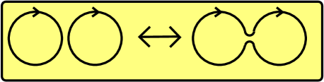
Figure 1: The ${\mathbb{Z}}_{2}$ twist field induces the usual splitting/joining interaction between strings, i.e. an interaction term that is cubic in the string fields.

In [13] it was shown that the leading irrelevant operator in this $g_{\mathrm{string}}$ expansion is given by a specific excited ${\mathbb{Z}}_{2}$ twist field ${\cal O}_{ij}$ that permutes pairs of two eigenvalue strings $x_{i}$ and $x_{j}$. In section 2 we show that this DVV twist field exactly reproduces the Lorentz-invariant Mandelstam vertex that describes the joining and splitting of type II strings in light-cone gauge, including the “prefactor”. Since the total scaling dimension of this twist field is $3$, this deformation is of first order in the string coupling by the scaling argument above.

If we try to go beyond the leading order perturbation, we face a lot of issues. Since we flow up in the RG, various more irrelevant terms will appear through contact terms, and the question is to which extent the super Poincaré invariance constrains the effective action (2). The hope is that a crucial role is played by the large $N$ limit, and we want to analyze this point in more detail in sections 3 and 4.

1.1 A few more words on matrix string theory

The generic matrix string configurations locally break the gauge group $U(N)$ to $U(1)^{N}$. The coefficient of the commutator terms diverges for $g_{\mathrm{string}}\to 0$ and therefore dynamics of the gauge theory involves the moduli space only: in the typical configurations, $X^{i}(\sigma)$ can be simultaneously diagonalized for each value of $\sigma$. However the basis in which they can be diagonalized may undergo a permutation if $\sigma$ increases by $2\pi$ (the periodicity) because a diagonal matrix conjugated by a permutation is again a diagonal matrix, and the symmetric group of permutations is a subgroup of the $U(N)$ gauge group. Therefore, in the $g_{\mathrm{string}}\to 0$ limit, low energy states of the gauge theory are divided into sectors classified by a permutation in $S_{N}\subseteq U(N)$. In other words, we deal with a two-dimensional theory on the orbifold

$${\mathbb{R}}^{8N}/S_{N}$$ (3)

with the appropriate number of fermionic fields to preserve ${\cal N}=8$ world sheet supersymmetry. The twisted sectors of the orbifold (3) are classified by a permutation. Every permutation may be factorized into a product of commuting cycles of length $n_{i}$ and the corresponding state describes a collection of strings whose longitudinal momenta equal $p^{+}_{i}=n_{i}/R$. Furthermore, the orbifold (3) requires us to omit the unphysical states which are not invariant under the $S_{N}\subseteq U(N)$ gauge transformations. For a given state, this constraint is nontrivial if we choose the permutation to be one of the generators of a ${\mathbb{Z}}_{n_{i}}$ group that cyclically permutes a given cycle. In the large $N$ limit, the ratios $n_{i}/N$ are kept fixed and $n_{i}$ are large. The group ${\mathbb{Z}}_{n_{i}}$ approximates the $U(1)$ group of rigid transformations of a long string. This implies that only the states that satisfy $L_{0}-\widetilde{L}_{0}=0$ appear in the physical spectrum [13].

Once we consider $g_{\mathrm{string}}$ small but finite, the strings can interact. Locally a $U(2)_{ij}$ group, originally broken to $U(1)_{i}\times U(1)_{j}$, can get restored. The detailed physics is a strongly coupled phenomenon from the gauge theory viewpoint; an instanton configuration that might be relevant in this context was suggested in [20, 21]. But the result of such a process may include the transposition of the $i$-th and $j$-th copy of the CFT; $i,j=1\dots N$. Such a transposition, when added to the original permutation, can join two cycles into one or split one cycle into two. This basic mechanism is responsible for stringy interactions [11].

We will often consider the Hamiltonian instead of the Lagrangian; for the leading order interaction to be described below the identity ${\cal H}=-{\cal L}$ may be applied. The Hamiltonian for the orbifold CFT, that approximates the $U(N)$ supersymmetric gauge theory on ${\mathbb{R}}\times S^{1}$, can be written as

$$P^{-}=\int_{0}^{1}{\rm d}\sigma\sum_{m=1}^{N}\left[(p_{m}^{i}(\sigma))^{2}+(x^{\prime i}_{m})^{2}+i\theta^{\prime}_{m}\Gamma_{9}\theta_{m}(\sigma)\right]+P^{-}_{\mathrm{interaction}}.$$ (4)

Here $\theta$ is a 16-component spinor of $SO(9)$, inherited from the BFSS model, that decomposes into ${\bf 8_{s}}\oplus{\bf 8_{c}}$ under the $SO(8)$ subgroup according to the eigenvalue of $\Gamma_{9}$; this eigenvalue decides whether the fermion becomes left-moving or right-moving. The type IIB D1-brane in the static gauge correctly reproduces the physics of the type IIA fundamental string in the light cone gauge.

What about the interactions? The leading term is the least irrelevant operator preserving the ${\cal N}=(8,8)$ world sheet (or Yang-Mills) supersymmetry:

$${L}_{\mathrm{interaction}}=g_{\mathrm{string}}\int_{0}^{L}{\rm d}\sigma\sum_{m<n}^{1\dots N}(\tau^{i}\Sigma^{i})_{m,n}\otimes(\bar{\tau}^{j}\bar{\Sigma}^{j})_{m,n}\quad+\quad O(g_{\mathrm{string}}^{2})$$ (5)

where the excited twist field operator $\tau^{i}$, $i=1,2,\dots 8_{v}$ and the spin field operators $\Sigma_{i}$ create a branch cut in the conformal field theory $CFT_{m}-CFT_{n}$, i.e. the sigma model with coordinates $x_{m}^{i}-x_{n}^{i}$. The orthogonal theory $CFT_{m}+CFT_{n}$ (as well as the other $CFT_{i}$’s for $i\neq m,n$) is not affected by the permutation of $m$ and $n$. Note that the interaction factorizes into the left-moving and the right-moving part. The integrand is an operator of dimension $(3/2,3/2)$. The total dimension is therefore mass³. Because the operator is integrated over ${\rm d}^{2}\sigma$ to obtain the action, its coefficient must have a dimension of the world sheet length. Since the only local distance scale of the gauge theory is $1/g=g_{\mathrm{string}}L$ where $L$ is the circumference of the $S^{1}$ in the gauge theory (it is equal to the inverse mass of the W-bosons that would have to be integrated out in order to obtain the interaction term), the gauge theory automatically generates the correct coefficient of (45) proportional to $g_{\mathrm{string}}$.

Now we want to remind the reader why the operator in (45) has dimension $(3/2,3/2)$. It is a product of a left-moving and a right-moving piece and therefore it is sufficient to show that $\tau^{i}\Sigma^{i}$ has dimension $3/2$. Although bosonic string theory cannot be written as a limit of a consistent gauge theory (because various supersymmetric cancellations are necessary for the matrix model to have a spacetime interpretation, i.e. to satisfy the cluster property), it is useful to consider the case of bosonic string theory first. In this case, $\tau^{i}\Sigma^{i}$ would be simply replaced by $\sigma$ (and $\bar{\tau}^{i}\bar{\Sigma}^{i}$ by $\bar{\sigma}$), the unexcited twist field:

$$\sigma=\prod_{i=1}^{24}\sigma^{(i)}$$ (6)

It has also dimension $24/16=3/2$ because $1/16$ comes from every transverse dimension. (The constant $1/16$ equals the difference between the zero point energy $+1/48$ in the antiperiodic sector and $-1/24$ in the periodic sector.) In the superstring case we must also add a spin field because fermions in $CFT_{m}$ and $CFT_{n}$ must get interchanged, too. But if the fermions $\theta^{a}$ transform in ${\bf 8_{s}}$ of $Spin(8)$, their spin fields must transform in ${\bf 8_{v}}\oplus{\bf 8_{c}}$, i.e. they are $\Sigma^{i}$ and $\Sigma^{{\dot{a}}}$. If we used $\Sigma^{\dot{a}}$, there would be no chance to contract the spinor index in order to create an $SO(8)$ invariant expression. Therefore we must choose $\Sigma^{i}$ and its vector index can be contracted with the vector index of the excited twist field $\tau^{i}$, corresponding to the vertex operator of the state

$$\alpha^{i}_{-1/2}\left|0\right\rangle_{\mbox{\scriptsize antiperiodic }x^{i}}\leftrightarrow\tau^{i}.$$ (7)

The total dimension of $\tau^{i}$ is $3/2$: $8/16$ comes from the spin field $\Sigma_{i}$, $8/16$ comes from the twist field $\sigma$ and $1/2$ comes from the excitation $\alpha_{-1/2}^{i}$ in (7). The resulting excited twist field $\tau^{i}\Sigma^{i}$ may be written as a supervariation, $\tau^{i}\Sigma^{i}=G^{\dot{a}}_{-1/2}(\sigma\Sigma^{\dot{a}})$.

Furthermore in the case of heterotic strings, we can combine a left-moving bosonic $\sigma$ with a right-moving supersymmetric $\bar{\tau}^{i}\bar{\Sigma}^{i}$. Because both factors have dimension $3/2$, we again obtain a $(3/2,3/2)$ operator [23]. This fact is important to preserve the correct scaling (1) of the interactions also for the heterotic matrix strings [24, 25].

1.2 A short review of Green-Schwarz superstring field theory

Light-cone gauge (super)string field theory is obtained by canonical second quantization of the first-quantized quantum mechanics of a single string. The amplitudes $\langle u|\psi\rangle$ become operators $\langle u|\hat{\Psi}\rangle$ that satisfy the commutation relations

$$[\langle u|\hat{\Psi}\rangle\,,\,\langle\hat{\Psi}|v\rangle]_{\mathrm{grad}}=\langle u|v\rangle.$$ (8)

The annihilation operators $\Psi_{u}=\langle u|\hat{\Psi}\rangle$—and analogously their Hermitian conjugates, the creation operators $\Psi^{\dagger}_{v}=\langle\hat{\Psi}|v\rangle$—can be written in terms of various bases of the first quantized Hilbert space, for instance a continuous functional basis, namely as string fields $\hat{\Psi}[x^{i}(\sigma),\theta^{a}(\sigma)]$ that depend on curves in a (super)space much like the fields in point-like particle quantum field theories depend on points in a (super)space.

The second-quantized kinematical generators and the free Hamiltonian are formally written as the expectation values in the string field operator-vectors, for example

$$P^{-}_{\mathrm{free}}\equiv H_{\mathrm{free}}=\langle\hat{\Psi}|h_{\mathrm{free}}|\hat{\Psi}\rangle=\sum_{u,v}\langle\hat{\Psi}|v\rangle\langle v|h_{\mathrm{free}}|u\rangle\langle u|\hat{\Psi}\rangle.$$ (9)

The interaction Hamiltonian of string field theory annihilates one string and creates two or vice versa; see figure 1. In the case of bosonic string field theory, it would have the form

$$g_{\mathrm{string}}\int{\cal D}z_{1}[\sigma]{\cal D}z_{2}[\sigma]{\cal D}z_{3}[\sigma]\Delta[z_{3}(\sigma)\!-\!z_{1}(\sigma)\!-\!z_{2}(\sigma)]\Psi^{\dagger}[z_{3}(\sigma)]\Psi[z_{1}(\sigma)]\Psi[z_{2}(\sigma)]$$ (10)

plus the Hermitean conjugate term, where the schematically written $\Delta$ functional is nonzero only if two parts of the string no. 3 overlap with the string no. 1 or the string no. 2, respectively. This continuity condition is automatically satisfied by the twist field $\sigma$ of the bosonic version of matrix string theory. The bosonic string interaction vertex contains no prefactors. This reflects the fact that the interactions of closed bosonic fields can have non-derivative character (for instance the tachyon potential term $T^{3}$).

The vertex in superstring field theory is more complicated. It contains a “prefactor” ${\cal H}$, an operator inserted at the interaction point. This prefactor is bilinear in the bosonic fields $\partial z^{i}(\sigma_{\mathrm{interaction}})$. This reflects the 2-derivative character of closed superstring field interactions (e.g. $\Phi R$ and $C\wedge F\wedge F$ in supergravity).

$$g_{\mathrm{string}} \int{\cal D}z_{1}^{\oplus}[\sigma]{\cal D}z_{2}^{\oplus}[\sigma]{\cal D}z_{3}^{\oplus}[\sigma]$$ (11)

$${\cal H}[z^{\oplus}(\sigma_{\mathrm{interaction}})]\Delta[z_{3}^{\oplus}(\sigma)\!-\!z_{1}^{\oplus}(\sigma)\!-\!z_{2}^{\oplus}(\sigma)]\Psi^{\dagger}[z_{3}^{\oplus}(\sigma)]\Psi[z_{1}^{\oplus}(\sigma)]\Psi[z_{2}^{\oplus}(\sigma)]\quad\,$$ (12)

Here ${\cal D}z^{\oplus}$ indicates the integral over the whole superspace, i.e. ${\cal D}^{8}z\,{\cal D}^{8}\Lambda$ where $\Lambda^{a}(\sigma)$ will denote eight fermionic coordinates.

The prefactor [26] is a polynomial

$${\cal H}=v^{ij}(\Lambda^{a}_{\mathrm{reg}})p_{\mathrm{reg}}^{i}\widetilde{p}_{\mathrm{reg}}^{j}.$$ (13)

Here the function $v^{ij}(\Lambda^{a})$ is an octic polynomial in the fermions near the interaction point, and

$$p_{\mathrm{reg}}^{i}\sim\sqrt{\epsilon}\partial z^{i}(\sigma_{\mathrm{interaction}}+\epsilon), \widetilde{p}_{\mathrm{reg}}^{j}\sim\sqrt{\epsilon}\bar{\partial}z^{i}(\sigma_{\mathrm{interaction}}+\epsilon)$$ (14)

$$\Lambda^{a}_{\mathrm{reg}}\sim\sqrt{\epsilon}\Lambda^{a}(\sigma_{\mathrm{interaction}}+\epsilon)$$ (15)

The operators $\partial z^{i}(\sigma),\bar{\partial}z^{i}(\sigma),\Lambda^{a}(\sigma)$ are singular at the interaction point, and therefore they must be evaluated at $\sigma_{\mathrm{interaction}}+\epsilon$ and multiplied by $\sqrt{\epsilon}$. The singular behavior can be seen if we use the coordinate $w$ that is related to $z$ by $z=w^{2}$: $\partial_{w}z^{i}(w)$ is finite in the $w$-plane (even around $w=0$), and therefore $\partial_{z}z^{i}(z)$ scales as $1/\sqrt{z}$. A generalization of the $w$-plane was employed by Wynter [22] to understand the nature of matrix string interactions.

Because an excited version of the twist field $\sigma$ is inserted at the interaction point, the factor $\sqrt{\epsilon}$ is precisely the factor needed to compensate $1/\sqrt{z}$ in the OPE of $\sigma$ with $\partial z^{i}$. In other words, $p_{\mathrm{reg}}^{i}$ is proportional to $\alpha_{-1/2}^{i}$. Clearly, the factor $p_{\mathrm{reg}}^{i}$ in (13) transforms $\sigma$ (corresponding to the bare delta functional) into $\tau^{i}$, an excited twist field. The factor $\widetilde{p}_{\mathrm{reg}}^{j}$ transmutes $\widetilde{\sigma}$ into $\widetilde{\tau}^{j}$ in a similar manner.

If we consider the equivalence between the $\sigma$ twist field in bosonic matrix string theory and the bosonic superstring field theory’s interaction vertex (containing no prefactors) to be a direct consequence of the topology of this interaction (strings split and join, as on figure 1), the remaining fact to be shown is that the function $v^{ij}(\Lambda^{a}_{\mathrm{reg}})$ from (13) describes the correct fermionic twist field $\Sigma^{i}\widetilde{\Sigma}^{j}$. The fermionic zero modes cause the unexcited fermionic twist field to be degenerate; it has $({\bf 8_{v}}+{\bf 8_{c}})\otimes({\bf 8_{v}}+{\bf 8_{c}})$ components: the left-moving part can be either $\Sigma^{i}$ or $\Sigma^{\dot{a}}$ and the right-moving part can be $\widetilde{\Sigma}^{i}$ or $\widetilde{\Sigma}^{\dot{a}}$. The space of functions of eight fermions $\Lambda^{a}$ is also 256-dimensional. Our task will be to show that $v^{ij}$ corresponds exactly to $\Sigma^{i}\widetilde{\Sigma}^{j}$.

2 The equivalence of the interaction vertices

It has become a well-known fact from matrix string theory that the large $N$ limit of the Hilbert space of the symmetric orbifold CFT reproduces the Hilbert space of the second-quantized superstring field theory in the light-cone gauge. The Hilbert space of large $N$ matrix string theory contains states with an arbitrary number of strings with arbitrary values of $P^{+}$ (while the total $P^{+}$ is fixed). The states must be invariant under the orbifold group. This has several consequences: the unbroken cyclical group ${\mathbb{Z}}_{k}$ commuting with a cycle of length $k$ becomes $U(1)$ generated by $L_{0}-\widetilde{L}_{0}$ when $k$ is large, and therefore the individual physical strings are guaranteed to satisfy $L_{0}=\widetilde{L}_{0}$. If several ($M_{k}$) strings (blocks) carry the same value of $k$, the unbroken group ${\mathbb{Z}}_{M_{k}}$ exchanging these strings imposes the (anti)symmetry of the wave function: strings in the same state are identical, with the correct statistics determined by their spin.

In this section we would like to explicitly show that the ${\mathbb{Z}}_{2}$ twist field describing the leading perturbation in matrix string theory coincides with the cubic interaction term in string field theory. The reader who is primarily interested in the higher order twist fields should skip this section.

Although the easiest theory to derive from the matrix description is type IIA string theory, we will be focusing on type IIB string theory. The twist field for type IIB string theory is completely analogous to that of type IIA string theory; the only difference is that the chirality of the left-moving fermions in all relevant formulae is inverted. All $\theta^{a}$ as well as $\widetilde{\theta}^{a}$ will have undotted indices.

This choice allows us to compare the twist field expressions with the formalism for string field theory by Green, Schwarz, and Brink [26] that pairs up eight real left-moving fermions with eight right-moving fermions into eight complex fermions and their conjugate momenta. It has the virtue of keeping the $spin(8)$ symmetry manifest. The equivalence of the two descriptions of type IIA superstring theory then follows from T-duality whose action is simple on both sides.

2.1 Identification of the unit function of fermions in the DVV language

Let us start with some useful and elementary OPEs of the fermions $\theta$ and their twist fields $\Sigma$:

$$\theta^{a}(z)\Sigma^{i}(0)\sim\frac{\eta^{*}}{\sqrt{2z}}\gamma^{i}_{a\dot{a}}\Sigma^{\dot{a}},\qquad\theta^{a}(z)\Sigma^{\dot{a}}(0)\sim\frac{\eta^{*}}{\sqrt{2z}}\gamma^{i}_{a\dot{a}}\Sigma^{i}.$$ (16)

We chose an equal phase $\eta^{*}=\mbox{exp}(-i\pi/4)$ in both numerators but this phase must be nontrivial in order to satisfy (18): one can derive this phase by the requirement that $\theta^{\langle a}\theta^{b\rangle}(z)$ acts as the same $SO(8)$ generator on $\theta^{c}(0)$ as well as all the $\Sigma$’s.

We define the antiholomorphic quantities in such a way that they satisfy the following OPEs (which differ by $z\leftrightarrow\bar{z}$ and $\theta\leftrightarrow\widetilde{\theta}$ etc. from (16), without changing the order of factors):

$$\widetilde{\theta}^{a}(\bar{z})\widetilde{\Sigma}^{i}(0)\sim\frac{\eta^{*}}{\sqrt{2\bar{z}}}\gamma^{i}_{a\dot{a}}\widetilde{\Sigma}^{\dot{a}},\qquad\widetilde{\theta}^{a}(\bar{z})\widetilde{\Sigma}^{\dot{a}}(0)\sim\frac{\eta^{*}}{\sqrt{2z}}\gamma^{i}_{a\dot{a}}\widetilde{\Sigma}^{i}.$$ (17)

We inserted the factors of $1/\sqrt{2}$ so that the OPEs are consistent with

$$\theta^{a}(z)\theta^{b}(0)\sim\frac{\delta^{ab}}{z},\quad\widetilde{\theta}^{a}(\bar{z})\widetilde{\theta}^{b}(0)\sim\frac{\delta^{ab}}{\bar{z}}.$$ (18)

In these calculations, $\theta^{a}$ is an anticommuting object. The spin field $\Sigma^{i}$ is treated as an anticommuting object, too, because it corresponds to $\psi^{i}$ in the RNS formalism. However $\Sigma^{\dot{a}}$ then must be a commuting object because of (16).

The periodic sector of eight pairs of fermions $\theta^{a},\widetilde{\theta}^{a}$ contains $({\bf 8_{v}}+{\bf 8_{c}})\otimes({\bf 8_{v}}+{\bf 8_{c}})$ states (of the supergravity multiplet) whose vertex operators are

$$\Sigma^{i}\widetilde{\Sigma}^{j},\quad\Sigma^{i}\widetilde{\Sigma}^{\dot{b}},\quad\Sigma^{\dot{a}}\widetilde{\Sigma}^{j},\quad\Sigma^{\dot{a}}\widetilde{\Sigma}^{\dot{b}}.$$ (19)

However in the $SO(8)$ invariant formalism for the light-cone gauge type IIB superstring field theory of Green, Schwarz, and Brink [26] we must pair the left-moving fermions and the right-moving fermions into superspace coordinates $\vartheta^{a}$ and superspace momenta $\lambda^{a}$:

$$\vartheta^{a}(\sigma)\approx\eta^{*}[S_{L}^{a}(\sigma)+iS_{R}^{a}(\sigma)],\qquad\lambda^{a}(\sigma)\equiv\frac{\partial}{\partial\vartheta^{a}(\sigma)}=\eta[S_{L}^{a}(\sigma)-iS_{R}^{a}(\sigma)].$$ (20)

There are eight complex fermionic coordinates $\vartheta^{a}$ at each point. The fields $S_{L},S_{R}$ are taken to be proportional to $\theta,\widetilde{\theta}$; also, a new symbol $\Lambda$ will be used for $\vartheta$ (up to an overall multiplicative factor). Because the three-string vertex contains a prefactor inserted at the interaction point, we must study the correspondence between the polynomials of $\vartheta(\sigma_{\mathrm{interaction}})$ and the operators (19). Which operator corresponds to the unit function of $\vartheta^{a}(\sigma)$, for example? Because the GSB formalism is $SO(8)$ invariant, the unit function must also be $SO(8)$ invariant. It is not hard to guess that it will contain an equal mixture of $\Sigma^{i}{\widetilde{\Sigma}}^{i}$ and $\Sigma^{{\dot{a}}}{\widetilde{\Sigma}}^{{\dot{a}}}$:

$$1_{\vartheta}\leftrightarrow\Sigma^{i}{\widetilde{\Sigma}}^{i}-i\Sigma^{{\dot{a}}}{\widetilde{\Sigma}}^{{\dot{a}}}.$$ (21)

While the overall normalization is somewhat arbitrary (although correlated with other conventions), the relative phase $(-i)$ is important to guarantee the counterpart of the identity $\partial(\sqrt{2}\eta)/\partial\vartheta=0$ in terms of the OPEs:

$$\begin{array}[]{rcl}\eta\sqrt{2}\left(\theta^{a}(z)-i{\widetilde{\theta}}^{a}(\bar{z})\right)\left(\Sigma^{i}{\widetilde{\Sigma}}^{i}(0)-i\Sigma^{\dot{b}}{\widetilde{\Sigma}}^{\dot{b}}(0)\right)&\sim&z^{-1/2}\gamma^{i}_{a{\dot{a}}}\Sigma^{\dot{a}}{\widetilde{\Sigma}}^{i}(0)+i\bar{z}^{-1/2}\gamma^{i}_{a{\dot{a}}}\Sigma^{i}{\widetilde{\Sigma}}^{\dot{a}}\\ &-&\!iz^{-1/2}\gamma^{i}_{a{\dot{b}}}\Sigma^{i}{\widetilde{\Sigma}}^{\dot{b}}(0)-\bar{z}^{-1/2}\gamma^{i}_{a{\dot{b}}}\Sigma^{\dot{b}}{\widetilde{\Sigma}}^{i}\end{array}$$ (22)

This vanishes for $z=\bar{z}$ positive; the positive real $z$-axis is used to regulate the quantities that diverge at the interaction point.

2.2 The remaining polynomials of the fermionic variables

The remaining polynomials in $\vartheta^{a}=\theta^{a}(z)+i{\widetilde{\theta}}^{a}(\bar{z})$ can be computed easily. Because (16) and (17) imply that $\theta(z),{\widetilde{\theta}}(\bar{z})$ behave in a singular way near the spin field, we define new variables

$$\Lambda^{a}=\sqrt{\frac{z}{2}}\theta^{a}(z)+i\sqrt{\frac{\bar{z}}{2}}{\widetilde{\theta}}^{a}(\bar{z}).$$ (23)

These are clearly related to $\vartheta^{a}$, assuming $z$ real and positive. By a function of $\Lambda^{a}$, we will mean the limit for $z\to 0$ of the OPE of the operator (23) with the “unit” vertex operator (21). One can also check that the derivatives with respect to $\Lambda^{a}$ can be represented by

$$\frac{\partial}{\partial\Lambda^{a}}=\sqrt{\frac{z}{2}}\theta^{a}(z)-i\sqrt{\frac{\bar{z}}{2}}{\widetilde{\theta}}^{a}(\bar{z})$$ (24)

so that the required anticommutators $\{\frac{\partial}{\partial\Lambda^{a}},\Lambda^{b}\}=\delta^{ab}$ are satisfied when acting on the spin fields.

It is natural to start with the linear functions of $\theta^{a}$. In this case, the contributions from (22) simply double:

$$\Lambda^{a}\leftrightarrow\eta^{*}\gamma^{i}_{a{\dot{a}}}(\Sigma^{\dot{a}}{\widetilde{\Sigma}}^{i}-i\Sigma^{i}{\widetilde{\Sigma}}^{\dot{a}}).$$ (25)

Let us act on the previous result with $\Lambda^{b}$:

$$\Lambda^{b}\Lambda^{a}\leftrightarrow-i\gamma^{i}_{a{\dot{a}}}\gamma^{j}_{b{\dot{a}}}\Sigma^{\langle j}{\widetilde{\Sigma}}^{i\rangle}-\gamma^{i}_{a{\dot{a}}}\gamma^{i}_{b{\dot{b}}}\Sigma^{\langle{\dot{b}}}{\widetilde{\Sigma}}^{{\dot{a}}\rangle}.$$ (26)

Note that in this $ab$ antisymmetric object only terms antisymmetric in $ij$ and ${\dot{a}}{\dot{b}}$ appear; they form the adjoint 28-dimensional representation of $SO(8)$ in all three cases. It is straightforward to continue and add $\Lambda^{c}$:

$$\begin{array}[]{rcl}\Lambda^{c}\Lambda^{b}\Lambda^{a}&\leftrightarrow&\frac{-i\eta^{*}}{2}\left(\Sigma^{\dot{c}}{\widetilde{\Sigma}}^{k}+i\Sigma^{k}{\widetilde{\Sigma}}^{\dot{c}}\right)\left(\gamma^{\langle k}_{a{\dot{a}}}\gamma^{j\rangle}_{b{\dot{a}}}\gamma^{j}_{c{\dot{c}}}+\gamma^{i}_{a\langle{\dot{a}}}\gamma^{i}_{{\dot{c}}\rangle b}\gamma^{k}_{c{\dot{a}}}\right)\\ &=&i\eta^{*}u^{k{\dot{c}}}_{abc}\left(\Sigma^{\dot{c}}{\widetilde{\Sigma}}^{k}+i\Sigma^{k}{\widetilde{\Sigma}}^{\dot{c}}\right)\end{array}$$ (27)

The $\gamma$-matrices and the symbols $u^{k{\dot{c}}}_{abc}$ and $t^{kl}_{abcd}$ are defined in [26]. The quartic polynomial is the last one that we will compute.

$$\begin{array}[]{rcl}\Lambda^{d}\Lambda^{c}\Lambda^{b}\Lambda^{a}&\leftrightarrow&u^{k{\dot{c}}}_{\langle abc}\left(\gamma^{l}_{d\rangle{\dot{c}}}\Sigma^{(l}{\widetilde{\Sigma}}^{k)}+i\gamma^{k}_{d\rangle{\dot{d}}}\Sigma^{\dot{c}}{\widetilde{\Sigma}}^{\dot{d}}\right)\\ &=&t^{kl}_{abcd}\Sigma^{k}{\widetilde{\Sigma}}^{l}+iu^{k{\dot{c}}}_{\langle abc}\gamma^{k}_{d\rangle{\dot{d}}}\Sigma^{{\dot{c}}}{\widetilde{\Sigma}}^{\dot{d}}\end{array}$$ (28)

The other polynomials are related to those above by the Grassmann Fourier transform i.e. by adding/removing $\Lambda$’s using the epsilon symbol. If we define the operator $\mathfrak{CH}$ by

$$\mathfrak{CH}=\left(\Lambda^{1}-\frac{\partial}{\partial\Lambda^{1}}\right)\left(\Lambda^{2}-\frac{\partial}{\partial\Lambda^{2}}\right)\dots\left(\Lambda^{8}-\frac{\partial}{\partial\Lambda^{8}}\right)=\prod_{a=1}^{8}\sqrt{2\bar{z}}{\widetilde{\theta}}^{a}(\bar{z}),$$ (29)

it is straightforward to see that $\mathfrak{CH}^{2}=1$ and

$$\begin{array}[]{rcl}\mathfrak{CH}(\Lambda^{a_{8}}\dots\Lambda^{a_{9-k}})&=&\frac{1}{k!}\epsilon^{a_{1}\dots a_{8}}\Lambda^{a_{1}}\dots\Lambda^{a_{k}}(-1)^{k}\\ &=&\int\mbox{exp}\left(\sum_{i=1}^{8}\Lambda^{i}\Lambda^{\prime i}\right)(\Lambda^{\prime a_{8}}\dots\Lambda^{\prime a_{9-k}})d\Lambda^{\prime 8}d\Lambda^{\prime 7}\dots d\Lambda^{\prime 1}\end{array}$$ (30)

where $\epsilon^{12345678}=+1$. Note that our formulae follow the equations in the appendix D of [26] for $\alpha=2$. More precisely, our $\Lambda$ is related to theirs by

$$\Lambda^{a}=\sqrt{\frac{2}{\alpha}}\Lambda^{a}_{GSB}.$$ (31)

How does $\mathfrak{CH}$ act on operators such as (19)? It is an $SO(8)$ invariant operator with eigenvalues $\pm 1$ for ${\widetilde{\Sigma}}^{i}$ and ${\widetilde{\Sigma}}^{\dot{a}}$, respectively: the equation (29) implies that $\mathfrak{CH}$ acts on the tilded spin fields only and this operator differs from the chirality operator by a triality transformation.

Finally we consider the polynomials from [26]:

$$w^{ij}=\delta^{ij}+\frac{1}{4!}t^{ij}_{abcd}\Lambda^{a}\Lambda^{b}\Lambda^{c}\Lambda^{d}+\frac{1}{8!}\delta^{ij}\epsilon^{abcdefgh}\Lambda^{a}\Lambda^{b}\dots\Lambda^{h}$$ (32)

While $w^{ij}$ is the symmetric part of $v^{ij}=w^{ij}+y^{ij}$, the quantity $y^{ij}$ is the antisymmetric part:

$$y^{ij}=-\frac{i}{2}\gamma^{ij}_{ab}\Lambda^{a}\Lambda^{b}-\frac{i}{2\cdot 6!}\epsilon^{ab\dots h}\Lambda^{c}\Lambda^{d}\dots\Lambda^{h}.$$ (33)

The effect of the term in (32) proportional to the $\epsilon$-symbol is to get rid of the $\Sigma^{\dot{a}}{\widetilde{\Sigma}}^{\dot{b}}$ part of (21) while it doubles the first part $\Sigma^{j}{\widetilde{\Sigma}}^{i}$. Similarly, the last term in (33) cancels the last term in (26) but doubles the first term. The symbol $t^{ij}_{abcd}$ is automatically self-dual:

$$t^{ij}_{abcd}\equiv\gamma^{ik}_{\langle ab}\gamma^{jk}_{cd\rangle}=\frac{1}{4!}\epsilon^{abcdefgh}t^{ij}_{efgh}.$$ (34)

We obtain

$$\begin{array}[]{rcccl}{w^{ij}}&\leftrightarrow&(2\delta^{ij}\delta^{kl}+\frac{1}{4!}t^{ij}_{abcd}t^{kl}_{abcd})\Sigma^{k}{\widetilde{\Sigma}}^{l}&=&+8(\delta^{ik}\delta^{jl}+\delta^{il}\delta^{jk})\Sigma^{k}{\widetilde{\Sigma}}^{l}\\ \mbox{and}\quad y^{ij}&\leftrightarrow&-\gamma^{ij}_{ab}\gamma^{kl}_{ab}\Sigma^{k}{\widetilde{\Sigma}}^{l}&=&-8(\delta^{ik}\delta^{jl}-\delta^{il}\delta^{jk})\Sigma^{k}{\widetilde{\Sigma}}^{l}\end{array}$$ (35)

Therefore the sum admits an easy representation:

$$v^{ij}\equiv w^{ij}+y^{ij}\leftrightarrow 16\Sigma^{j}{\widetilde{\Sigma}}^{i}.$$ (36)

It is equally straightforward to translate the fermionic functions into the spin field representation:

$$\begin{array}[]{rcl}s_{1}^{i{\dot{a}}}&=&2\gamma^{i}_{a{\dot{a}}}\Lambda^{a}+\frac{1}{3\cdot 5!}u^{i{\dot{a}}}_{abc}\epsilon^{ab\dots h}\Lambda^{d}\Lambda^{e}\dots\Lambda^{h}\\ s_{2}^{i{\dot{a}}}&=&-\frac{1}{3}u^{i{\dot{a}}}_{abc}\Lambda^{a}\Lambda^{b}\Lambda^{c}+\frac{2}{7!}\gamma^{i}_{a{\dot{a}}}\epsilon^{ab\dots h}\Lambda^{b}\Lambda^{c}\dots\Lambda^{h}.\end{array}$$ (37)

Let us consider the combination

$$\frac{\eta}{2}(s_{1}^{i{\dot{a}}}-is_{2}^{i{\dot{a}}})\leftrightarrow\left(2\gamma^{i}_{a{\dot{a}}}\gamma^{k}_{a{\dot{c}}}+\frac{1}{3}u^{i{\dot{a}}}_{abc}u_{abc}^{k{\dot{c}}}\right)\Sigma^{{\dot{c}}}{\widetilde{\Sigma}}^{k}=16\Sigma^{{\dot{a}}}{\widetilde{\Sigma}}^{i}$$ (38)

This operator is important for the interaction part of the dynamical supersymmetry operator. In a complete analogy one can also construct the other combination:

$$-\frac{\eta^{*}}{2}(s_{1}^{i{\dot{a}}}+is_{2}^{i{\dot{a}}})\leftrightarrow\left(2\gamma^{i}_{a{\dot{a}}}\gamma^{k}_{a{\dot{c}}}+\frac{1}{3}u^{i{\dot{a}}}_{abc}u_{abc}^{k{\dot{c}}}\right)\Sigma^{k}{\widetilde{\Sigma}}^{\dot{c}}=16\Sigma^{i}{\widetilde{\Sigma}}^{\dot{a}}$$ (39)

Type IIB string theory allowed us to use a $Spin(8)$ invariant formalism for string field theory; this is also possible for its orientifold, type I string theory. Type IIA and heterotic string field theories require us to use a formalism that breaks $Spin(8)$. The twist field formalism, on the other hand, keeps $Spin(8)$ manifest. The proof of equivalence in the other cases could be nevertheless performed in a direct analogy with the type IIB proof above.

3 The large $N$ scaling limit

We now turn to the role of the large $N$ scaling limit in conformal perturbation theory around the $S^{N}{\mathbb{R}}^{8}$ orbifold model. Note that in contrast with the ’t Hooft limit, where one keeps $g^{2}N$ fixed and is driven to weak coupling $g\to 0$ as $N\to\infty$, in the large $N$ limit the dimensionless Yang-Mills coupling constant $gL=1/g_{\mathrm{string}}$ remains fixed. Therefore the usual perturbative large $N$ techniques do not apply.

Furthermore, one should take into account that only Yang-Mills energies of the order $1/N$ can give rise to finite spacetime energy in the light-cone frame. The truncation to these extremely low-lying states can be implemented by a rescaling of the worldsheet time coordinate $\tau$ by a factor of $N$:

$$\tau\to N\tau.$$ (40)

The appearance of energies of order $1/N$ in the supersymmetric gauge theory has an intuitive explanation in the strong coupling IR phase where the ‘long string’ configurations dominate. In this regime the matrix-valued coordinates $X^{i}$ commute almost everywhere, where they can be simultaneously diagonalized giving $N$ eigenvalue vectors $x_{1}^{i},\dots,x_{N}^{i}$. The long strings are made up of twisted configurations of these eigenvalue strings or string bits: the twisted sector corresponding to a permutation $p\in S_{N}\subset U(N)$ describes a configuration of strings of lengths $n_{i}$ where

$$p=\prod_{i=1}^{N_{\mathrm{cycles}}}(n_{i}),\qquad\sum_{i=1}^{N_{\mathrm{cycles}}}n_{i}=N$$ (41)

where $(n_{i})$ are the independent cycles of the permutation that generate ${\mathbb{Z}}_{n_{i}}$ subgroups of $S_{N}$. These residual groups ${\mathbb{Z}}_{n_{i}}$ are part of the gauge group that must keep physical states invariant. This fact imposes the constraints for the individual strings

$$L_{0}(i)-\widetilde{L}_{0}(i)\in n_{i}{\mathbb{Z}}.$$ (42)

For $N\to\infty$ and $n_{i}/N$ fixed, $n_{i}\to\infty$ guarantees that the finite energy configurations must satisfy $L_{0}(i)-\widetilde{L}_{0}(i)=0$. If two strings with $n_{i}=n_{j}$ are excited in the same state $|\psi\rangle$, an extra permutation exchanging these two cycles guarantees that the wave function is (anti)symmetric, according to the statistics of $|\psi\rangle$.

The worldsheet of the long strings is an $N$-fold cover of the cylinder on which the Yang-Mills theory is defined. These covering Riemann surfaces have circumference $NL$ and they can support fractional momenta $\sim 1/N$. The appearance of these long strings is therefore a crucial ingredient in our understanding why the large $N$ limit of Matrix theory leads to a non-trivial scaling limit of the SYM theory. Note that, since we also scaled the worldsheet time $\tau$ by a factor of $N$, one can think of the perturbative string worldsheets as scaled by an overall factor of $N$ compared to the SYM cylinder. So scaling in $N$ can be thought of in terms of RG flow—a point of view that we will further explore.

3.1 The renormalization group involving $N$

The leading perturbation is an irrelevant twist field and a natural question is why such an irrelevant operator affects physics at very long worldsheet distances. The subtlety that makes this twist field important is an extra scaling with $N$.

The light-cone Hamiltonian for the orbifold CFT, that approximates the $U(N)$ supersymmetric gauge theory on ${\mathbb{R}}\times S^{1}$, can be written as

$$P^{-}=\int_{0}^{L}{\rm d}\sigma\sum_{m=1}^{N}\left[(p_{m}^{i}(\sigma))^{2}+(x^{\prime i}_{m})^{2}+i\theta^{\prime}_{m}\Gamma_{9}\theta_{m}(\sigma)\right]+P^{-}_{\mathrm{interaction}}.$$ (43)

Here $\theta$ is a 16-component spinor of $SO(9)$, inherited from the BFSS model, that decomposes into the eigenvectors of the chirality matrix $\Gamma_{9}$, i.e. ${\bf 8_{s}}\oplus{\bf 8_{c}}$ under the $SO(8)$ subgroup. The type IIB D1-brane in the static gauge correctly reproduces the physics of the type IIA fundamental string in the light cone gauge.

If the light-like radius $R_{-}$ becomes infinite and $p^{+}$ is kept fixed i.e. $N\to\infty$, the DLCQ treatment becomes ordinary light-cone gauge quantization and the length of string bits $L$ becomes infinitesimal compared to the total length of the strings $NL$. We see that the free term in (43) may be rewritten as an integral over the string(s) of length $NL$:

$$P^{-}=\int_{0}^{NL}{\rm d}\sigma\left[(p^{i}(\sigma))^{2}+(x^{\prime i})^{2}+i\theta^{\prime}\Gamma_{9}\theta(\sigma)\right]+P^{-}_{\mathrm{interaction}}.$$ (44)

What about the interactions? The leading term is the least irrelevant operator preserving the ${\cal N}=(8,8)$ world sheet (or Yang-Mills) supersymmetry:

$$P^{-}_{\mathrm{interaction}}=\frac{1}{g}\int_{0}^{L}{\rm d}\sigma\sum_{m<n}^{1\dots N}(\tau^{i}\Sigma^{i})_{m,n}\otimes(\bar{\tau}^{j}\bar{\Sigma}^{j})_{m,n}\quad+\quad O(g_{\mathrm{string}}^{2})$$ (45)

In this form, the interaction term, resulting from a strongly coupled dynamics where $U(2)_{m,n}$ (otherwise broken to $U(1)\times U(1)$) gets restored, there is no $N$-dependence but the term must be summed over $m,n$. The Yang-Mills coupling constant $g$ (of dimension mass) determines the only local scale of Yang-Mills theory and the appropriate power is inserted on dimensional grounds because the twist field has total dimension $3$. As $N$ becomes large, the interaction can effectively occur between any two points on the string(s) and the continuum limit of (45) can therefore be written as a bilocal term

$$P^{-}_{\mathrm{interaction}}=\frac{1}{gL}\int_{0}^{NL}{\rm d}\sigma\int_{0}^{NL}{\rm d}\sigma^{\prime}(\tau^{i}\Sigma^{i})_{(\sigma,\sigma^{\prime})}\otimes(\bar{\tau}^{j}\bar{\Sigma}^{j})_{(\sigma,\sigma^{\prime})}\quad+\quad O(g_{\mathrm{string}}^{2})$$ (46)

Recall that the coefficient of this term is $1/gL=g_{\mathrm{string}}$. The expression (46) is locally $N$-independent.

More generally, if the twist field appearing in (45) has the usual RG dimension $d=h+\bar{h}$, the coefficient will be $1/g^{d-2}$ on dimensional grounds. If it connects $w$ indices, i.e. if the sum contains $O(N^{w})$ terms (the leading perturbation in (45) has $w=2$), then the continuum limit, giving a $w$-local (bilocal, trilocal, tetralocal etc.) interaction, requires us add a factor $1/L^{w-1}$. The total coefficient replacing $1/gL$ in (46) will be

$$\frac{1}{g^{d-2}L^{w-1}}=\frac{g_{\mathrm{string}}^{w-1}}{g^{d-1-w}}$$ (47)

The power of $g_{\mathrm{string}}$ is thus determined by $w-1$ only: the free Hamiltonian has $w=1$ and therefore no $g_{\mathrm{string}}$ dependence. The leading perturbation has $w=2$ and is therefore proportional to $g_{\mathrm{string}}$. The ${\mathbb{Z}}_{k}$ twist field, permuting $k$ eigenvalue strings, leads to a perturbation of order $g_{\mathrm{string}}^{k-1}$. Such a term in the action is generated by the strongly coupled gauge theory dynamics in which a group $U(k)$ gets restored.

The denominator in (47) is $g^{d-1-w}$. It is dimensionless if $d-1-w=0$. In this case, we will say that the twist field is $N$-marginal and its effects survive the continuum limit. If $d-1-w>0$, the coefficient $g^{-d+1+w}$ has dimension of a positive power of length, and therefore this term is $N$-irrelevant in the IR i.e. for long strings where we can essentially send $g\to\infty$. $N$-relevant operators would have to have $d-1-w<0$. Such operators are incompatible with supersymmetry, except for the (untwisted) mass terms that appear in the light-cone gauge description of strings in the pp-waves.

In other words, $(d+1-w)=(d-1-w)+2$ is the $N$-corrected dimension that takes the scaling of $N$ together with worldsheet distances into account. Only the $N$-marginal operators with $d-1-w=0$ survive the large $N$ i.e. $g\to\infty$ limit of matrix string theory. In the section 4 we will see that the leading supersymmetric $Spin(8)$ invariant twist field from the ${\mathbb{Z}}_{w}$ twisted sector is $N$-marginal.

Another argument in favor of the condition $d-1-w=0$ in flat space is the invariance under the boosts generated by $J_{+-}$ that rescale $P^{+}$ by $\kappa$ and $P^{-}$ by $1/\kappa$: the Hamiltonian $P^{-}$ must scale like $1/P^{+}$. The variables $\sigma$ scale just like $P^{+}$ because the length of the strings represents the light-like momentum. Therefore $w$ integrals over $\sigma$ in (46) scale like $(P^{+})^{w}$. An operator of dimension $d$ scales like $(P^{+})^{-d}$. The product $(P^{+})^{-d+w}$ must scale like $(P^{+})^{-1}$, and therefore $d-1-w=0$.

3.2 Moduli and powers of $N$

There is actually a direct link between the $N$ scaling of the interaction vertex and the moduli of the light-cone diagrams. Consider adding a handle to a particular diagram by two insertions of the twist field:

$$\int{\cal O}_{(IJ)}{\cal O}_{(KL)}.$$ (48)

Each operator ${\cal O}_{(IJ)}$ has dimension $3$ and scales therefore as $N^{-3}$. These three factors of $N$ are compensated by two integrals over $\sigma$ and one integral over $\tau$.

A product of two such operators (48) scales like $N^{-6}$. This factor must be cancelled by $6$ explicit factors of $N$. The integral over $6$ worldsheet variables has an interpretation in terms of moduli. Adding a handle to a Riemann surface generically adds $6$ new real moduli. In the light-cone gauge language, they can be interpreted as follows:

• two time coordinates $\tau,\tau^{\prime}$ of the interaction vertices

• one common position of the vertices in $\sigma$; it carries the information how $P^{+}$ is separated between two virtual strings

• three twist parameters $\Delta\sigma_{1,2,3}$ that implement the condition $L_{0}-\widetilde{L}_{0}=0$ on two new virtual “smaller” strings and one new “bigger” string

We claim that in DLCQ, each of these $6$ real moduli comes with a factor of $N$, and the total factor of $N^{6}$ compensates $N^{-6}$ from the dimensions of the twist fields. The factors of $N$ coming with the $\tau,\tau^{\prime},\sigma$ integrals have been explained previously. The projection to the states satisfying $L_{0}-\widetilde{L}_{0}=0$ is approximated by a ${\mathbb{Z}}_{n_{i}}$ projection and $n_{i}$ scales like $N$ as well. In fact, in this way we could identify the scaling dimension $3$ of the vertex, with the number $3$ appearing in the complex dimension $3h-3$ of the moduli space of Riemann surfaces of genus $h$.

This analysis can also be extended to include punctures. If the total number of external states is $n$, the number of vertices (pairs of pants) is given by minus the Euler character $(2h-2+n)$ leading to a total scaling dimension of $N^{-(6h-6+3n)}$. The number of real moduli is $6h-6+2n$. There is however an extra factor of $N$ for each external state, that implements the ${\mathbb{Z}}_{n_{i}}$ level-matching projection. The normalization with $N$ is natural both in the orbifold model (viewed as an $S_{N}$ gauge theory) and on the light-cone theory phase space (where the factors of $N$ are needed to give $\delta(p^{+})$ normalizations of the external states). So, altogether we obtain a combinatorial power $N^{6h-6+3n}$ that compensates precisely the scaling of the vertices.

Summarizing: the $N$ scaling weight of correlators in the orbifold SCFT agrees with the weight of the corresponding string amplitude viewed as an integral over the moduli space of light-cone diagrams.

Let us note that the ${\mathbb{Z}}_{2}$ twist field only has scaling dimension $3$ in the case of an 8-dimensional transverse space. This is how the critical dimension appears in the strong coupling gauge theory. It should be compared to the covariant formulation where the coordinate and ghost determinants only combine into a proper density over the (super)moduli space for the critical space-time dimension. Note that in the subcritical case of $D<8$ transverse dimensions the string coupling constant is $N$-relevant (the dimension is something like $1+D/4$) and will diverge in the large $N$ limit. This might be of relevance for the six-dimensional non-Abelian $(2,0)$ strings, that allow a matrix formulation in terms of sigma models on the $N$-instanton moduli space [7].

For a transverse $M^{4}$ (which is either $T^{4}$ or $K3$) this instanton moduli space is a hyperKähler deformation of a symmetric product, and part of the above analysis might apply.

Conformal field theory on a deformed symmetric product of many copies of $M^{4}$ is the dual description of type IIB string theory on $AdS_{3}\times S^{3}\times M^{4}$. The conformal symmetry implies that the deformation must be marginal in the ordinary sense, not $N$-marginal. In the pp-wave limit of the symmetric orbifold $S^{N}M^{4}$, one must combine the pp-wave string bit techniques [27] with matrix string theory to understand the full stringy Hamiltonian [28]. The reason that the marginal perturbation (the resolution of the fixed points of the symmetric orbifold) turns out also to be $N$-marginal is that a BMN-like mechanism renormalizes the kinetic terms in such a way that the worldsheet distances seem to be contracted by $g_{\mathrm{string}}Q_{5}$.

4 Twist fields and contact terms

Let us consider in more detail the large $N$ behavior of operators in the ${\mathbb{R}}^{8N}/S_{N}$ orbifold. Since the operators naturally factorize in a product of ${\mathbb{Z}}_{n_{i}}$ factors, it suffices to start with a single ${\mathbb{Z}}_{w}$ twist field. Such an operator cyclically permutes the coordinates $x_{1}^{i},x_{2}^{i},\dots,x_{w}^{i}$ of $w$ eigenvalue strings. In string perturbation theory this operator describes a vertex of order $w+1$ (or less by an even number) in the string fields.

The twist operator induces twisted boundary conditions for the bosons

$$x_{I}^{i}(\sigma+2\pi)=x^{i}_{I+1}(\sigma)$$ (49)

where $I+1$ is computed modulo $w$. The cyclic group element also acts on the left-moving as well as the right-moving fermions $\theta^{a}_{I}$ and $\bar{\theta}^{\dot{a}}_{I}$. With periodic (Ramond) boundary conditions, the action is

$$\theta^{a}_{I}(\sigma+2\pi)=\theta_{I+1}^{a}(\sigma)$$ (50)

whereas with antiperiodic (Neveu-Schwarz) boundary conditions we have

$$\theta^{a}_{I}(\sigma+2\pi)=-\theta_{I+1}^{a}(\sigma).$$ (51)

Similar relations hold for the right-movers. Note that the Ramond sector always has a $16\times 16$ degeneracy, since the linear sum

$$\sum_{I=1}^{w}\theta^{a}_{I}$$ (52)

is periodic and gives fermionic zero modes. In the Neveu-Schwarz sector the fermionic zero modes appear for even $w$ only and have the form

$$\sum_{I=1}^{w}(-1)^{I}\theta^{a}_{I}.$$ (53)

For $w$ odd the Neveu-Schwarz ground state is a singlet. This includes the NS vacuum in the untwisted sector $w=1$ as a special case.

It is not difficult to compute the scaling dimensions of the ground states in such ${\mathbb{Z}}_{w}$ twisted sectors. First of all, both for the bosons and the fermions the ${\mathbb{Z}}_{w}$ action can be diagonalized by taking complex linear combinations. (In the case of fermions, this only leaves the subgroup $SU(4)\times U(1)$ of $spin(8)$ manifest.)

The bosonic twist field that implements a twist with eigenvalue $e^{2\pi ik/w}$ where $k=0,1,\dots w-1$, is well-known to have the total (left+right) scaling dimension $Dk(w-k)/2w^{2}$ with $D$ the dimension of the transversal space (in our case of type II string theory, $D=8$). For the fermionic twist field with the same twist $e^{2\pi ik/w}$ ($k$ is an integer or half-integer for the NS or R sector respectively) we find dimension $Dm^{2}/2w^{2}$ where $m=\min(k,w-k)$.

Summing up all possible eigenvalues for $D=8$ we obtain a scaling dimension $w$ for the R ground states and

$$d=\left\{\begin{array}[]{ll}w,&w\mbox{\,\,\,even}\\ w-1/w,&w\mbox{\,\,\,odd}\end{array}\quad\right\rangle\quad\mbox{for the NS ground states.}$$ (54)

We are however only interested in those states that are invariant under the supersymmetry and $Spin(8)$. Although the NS ground states for $w$ odd are $Spin(8)$ invariant, they are not supersymmetric.

The least irrelevant invariant twist field ${\cal O}_{(w)}$ can be constructed analogously to the ${\mathbb{Z}}_{2}$ operator in [13]. Because of supersymmetry at the leading order in $g_{\mathrm{string}}$, it must be written as a supersymmetric descendent of a NS state with the correct indices $\dot{a},b$

$${\cal O}_{(w)}=G^{\dot{a}}_{-1/2}\bar{G}_{-1/2}^{b}{\cal O}_{(w)}^{\dot{a}b}.$$ (55)

For $w=2$ we obtain the leading perturbation (DVV twist field). More generally for $w$ even, ${\cal O}_{(w)}^{\dot{a}b}$ is exactly one of the degenerate ground state twist fields. However for $w$ odd (55) must be completed by a definition of ${\cal O}_{(w)}^{\dot{a}b}$ because the ground state ${\cal O}_{(w)}$ is non-degenerate in this case. The right prescription for ${\cal O}_{(w)}^{\dot{a}b}$ can be easily guessed in analogy with the case $w=1$ where

$$\partial x^{i}\bar{\partial}x_{i}=G_{-1/2}^{\dot{a}}\bar{G}_{-1/2}^{b}\gamma^{i}_{a\dot{a}}\gamma_{i,b\dot{b}}\theta^{a}\bar{\theta}^{\dot{b}}.$$ (56)

Because this is again a descendant, it is supersymmetric up to a total derivative. For general odd $w$ we can therefore define the least irrelevant operator appearing in (55) as

$${\cal O}_{(w)}^{\dot{a}b}=\gamma^{i}_{a\dot{a}}\gamma_{i,b\dot{b}}\theta_{-1/2w}^{a}\bar{\theta}^{\dot{b}}_{-1/2w}|0\rangle$$ (57)

where $|0\rangle$ denotes the unique ${\mathbb{Z}}_{w}$ NS ground state. One might also consider another operator of the same dimension as (57), namely $\theta_{-1/2w}^{b}\bar{\theta}^{\dot{a}}_{-1/2w}|0\rangle$, but it would transform incorrectly under supersymmetry; the operator $\gamma^{i}_{a\dot{a}}\gamma_{i,b\dot{b}}$ that projects the spinors onto their self-dual part seems to play a crucial role. The invariant operator ${\cal O}_{(w)}$ that is reproduced in this way has again total scaling dimension $w+1$, and therefore is $N$-marginal as described in the subsection 3.1. The operators then lead to the $g_{\mathrm{string}}^{w-1}$ dependence on the string coupling constant. The $S_{N}$ invariance implies that the term must be summed over the whole conjugacy class:

$$g_{\mathrm{string}}^{w-1}\int\mathrm{d}\sigma\sum_{I_{1}<\dots I_{w}}{\cal O}_{(I_{1}\dots I_{w})}.$$ (58)

All other supersymmetric and $Spin(8)$ invariant operators in the twisted sector are $N$-irrelevant, and therefore will become unimportant in the large $N$ limit. Intuitively it is not too surprising because such operators are obtained by acting with $\partial x^{i}$ on the operator ${\cal O}$ that leads to an extra factor of $1/N$ because of the long strings.

Note that the unique operator (55) replaces a whole family of different operators that one would have to insert in string field theory. For example the ${\mathbb{Z}}_{3}$ vertex induces the interactions from figure 2 and the higher-order diagrams would lead to an even larger set of interactions.

We mention that the operators of dynamical spacetime supercharges $Q^{-\dot{a}}$ and $\bar{Q}^{-b}$ contain terms similar to (55), but without one of the worldsheet supersymmetric excitation:

$${\cal O}_{(w)}^{\dot{a}}=\bar{G}_{-1/2}^{b}{\cal O}_{(w)}^{\dot{a}b},\quad\bar{\cal O}_{(w)}^{b}=G^{\dot{a}}_{-1/2}{\cal O}_{(w)}^{\dot{a}b}.$$ (59)

It would be interesting to compute the actual numerical coefficients of all the operators ${\cal O}_{(w)}$ in $P^{-},Q^{-\dot{a}},\bar{Q}^{-b}$. We believe that the expansion is non-polynomial, much like other closed string theory actions as well as their low energy limit, i.e. the Einstein-Hilbert action. The coefficients of the contact terms must be usually taken to be infinite, $1/\epsilon^{\alpha}$, and the circumference of the Yang-Mills cylinder $L$ will play the role of the natural worldsheet cutoff $\epsilon$ in our case.

4.1 An example: ${\mathbb{Z}}_{2}$ and ${\mathbb{Z}}_{3}$ twist fields and pp-waves

The ${\mathbb{Z}}_{2}$ twist field ${\cal O}_{(IJ)}$ has the interpretation of the three-string joining/splitting vertex (see the figure 1). The higher order twist fields describe spacetime contact terms that are known to appear in light-cone gauge perturbation theory [29, 30, 31, 32].

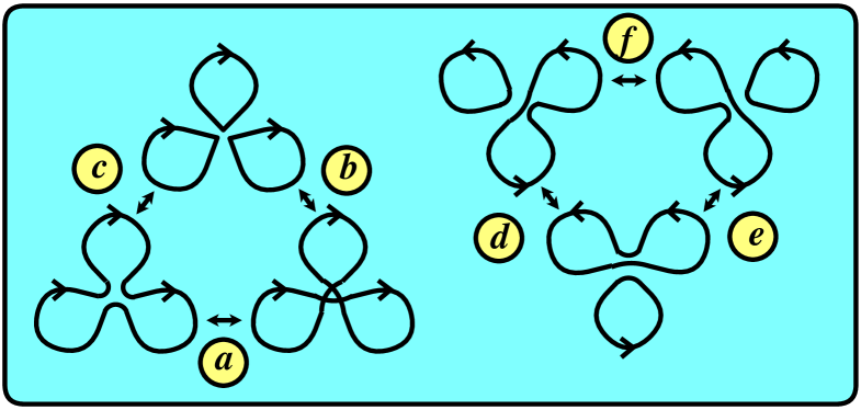
Figure 2: The ${\mathbb{Z}}_{3}$ twist field induces quadratic (a) and quartic (b,c,d,e,f) (depending on the choice of the twisted sector) contact interactions of the string fields. The local form of the trilocal interaction is identical in all cases. Higher order twist fields give rise to ever larger number of different string field interaction terms.

For example, locally the same ${\mathbb{Z}}_{3}$ vertex (that is an effective description of physical phenomena resulting from a $U(3)$ symmetry restoration) generates a quartic as well as a quadratic contact interaction (see figure 2) in the string fields that scales like $g_{\mathrm{string}}^{2}$. The quadratic interaction is necessary [29, 30, 32] to cancel the $g_{\mathrm{string}}^{2}$ self-energy of the supergraviton ground state in the second-order of the old-fashioned quantum perturbation theory which is known to be negative for the ground state:

$$E^{(2)}_{n}=\sum_{m}^{m\neq n}\frac{|V_{mn}|^{2}}{E_{n}^{(0)}-E_{m}^{(0)}}.$$ (60)

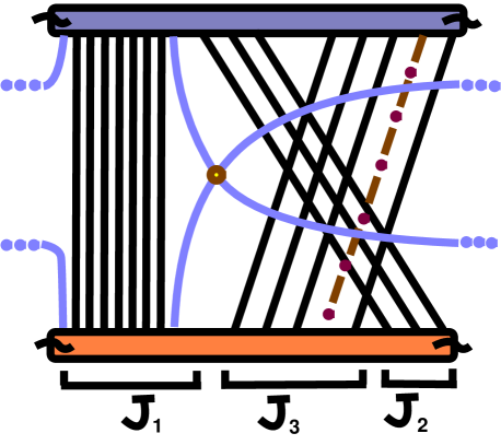
Figure 3: The non-nearest neighbor diagram from [34] contributing to a self-energy of a string has the form of the contact interaction from figure 2(a).

This is just a special case of a more general requirement that the super Poincaré algebra is closed at higher orders in $g_{\mathrm{string}}$; this requirement forces us to add higher order terms into the Hamiltonian and the dynamical supersymmetry generators.

A simple argument showing that these $g_{\mathrm{string}}^{2}$ terms are inevitable is the following: the ground state energy (i.e. the mass of the graviton multiplet) always acquires a negative shift in the second order perturbation theory, and an explicit positive shift proportional to $g_{\mathrm{string}}^{2}$ (see figure 2(a)) is needed to compensate this second-order correction and keep the graviton massless.

We can also see that the non-nearest neighbor diagrams of [34] (see also [33]) depicted on figure 3 that contribute to the self-energy of the states in the pp-wave background have exactly the structure of the quadratic ${\mathbb{Z}}_{3}$ contact interaction. (A string is divided to three pieces that get rearranged.) Note that the pp-wave deformation of string theory is relevant, and therefore does not affect the UV physics on the worldsheet. However, the exact analysis of the self-energy is more complicated because of the operator mixing effects [35, 36, 37, 38]. A general proposal to identify all the Feynman diagrams that are responsible for the contact terms appeared in section 5 of [39].

4.2 Composite operators

Up to now we only analyzed the operators in a single ${\mathbb{Z}}_{n}$ twisted sector. The full orbifold also contains twisted superselection sectors that are products of such cyclic permutations. In that case one simply takes the products of the operators of the individual factors. However, these composite operators are always $N$-irrelevant.

Consider a simple example: a conjugacy class of type $(IJ)(KL)$ with $I,J,K,L$ all different, consisting of two elementary transpositions. The obvious guess for the least-irrelevant operator in this sector is

$${\cal O}_{(IJ)(KL)}={\cal O}_{(IJ)}{\cal O}_{(KL)}.$$ (61)

Note that the OPE of the factors on the right hand side of (61) is non-singular because the twist fields act on different coordinates. It has total scaling dimension $6$ and combinatorial weight $4$, and therefore scales as $N^{-1}$. It is therefore $N$-irrelevant. One could also try other combinations, such as ${\cal O}^{\dot{a}b}_{(IJ)}{\cal O}_{(KL)}^{\dot{a}b}$ of weight four. This is $spin(8)$ invariant, but not supersymmetric.

In summary: it is only the irreducible ${\mathbb{Z}}_{n}$ vertices that survive the large $N$ scaling.

4.3 Contact terms on the worldsheet

The ${\mathbb{Z}}_{2}$ twist field ${\cal O}_{(IJ)}$ has an interpretation as the three-string joining/splitting vertex. The higher order twist fields describe spacetime contact terms, that are known to appear in light-cone perturbation theory. They are necessary for the supersymmetry algebra to be closed at higher orders in $g_{\mathrm{string}}$.

In fact, these terms also appear as worldsheet contact terms in the conformal perturbation theory. For example, in the OPE of two ${\mathbb{Z}}_{2}$ twist fields the ${\mathbb{Z}}_{3}$ twist field can appear through

$${\cal O}_{(IJ)}(z){\cal O}_{(JK)}(w)\sim\frac{1}{|z-w|^{2}}{\cal O}_{(IJK)}(w),\qquad I\neq K.$$ (62)

The singularity is logarithmic (just as in the OPE of marginal operators), so that in the RG flow the ${\mathbb{Z}}_{3}$ contact term ${\cal O}_{(IJK)}(w)$ is reproduced with a finite coefficient. So the effective action contains a term

$$g_{\mathrm{string}}^{2}\int\sum_{I<J<K}{\cal O}_{(IJK)}.$$ (63)

One easily verifies that in all OPEs between these least irrelevant invariant operators the singularities are of the above type. (Roughly because they are descendents of chiral primary fields.) Since all such operators are $N$-marginal, this contact term algebra is preserved in the large $N$ limit.

Note that in this way the ${\mathbb{Z}}_{n}$ twist fields for $n>2$ are made out of contact terms between the fundamental ${\mathbb{Z}}_{2}$ vertices, these higher order interactions also respect the 10-dimensional Lorentz symmetry!

5 Conclusions and outlook

We believe that the twist field formulation of perturbative string theory in the light-cone gauge is more natural and more fundamental than the usual language of second-quantized string field theory. A single and simple twist field at each order in $g_{\mathrm{string}}$ gives rise to many polynomial interactions of the string fields. Yet, it is still straightforward to translate the expressions involving twist fields into those involving string fields. Instead of complicated Neumann coefficients, one can study simple OPEs in a conformal field theory. A modified version of the renormalization group includes the $N$-scaling as well and helps us to understand the large $N$ limit that is responsible for the light-like decompactification limit of Matrix theory.

It could be interesting to:

• determine the precise coefficients of the ${\mathbb{Z}}_{n}$ twist fields from the requirement that the super Poincaré algebra is closed; are all the coefficients non-zero? A recent investigation of the pp-waves [44] seems to indicate that all terms beyond $g_{\mathrm{string}}^{2}$ vanish;

• compute the matrix elements of the contact terms between general string states;

• study the divergence of the string coupling expansion of the light-cone Hamiltonian itself; does it diverge in the same sense as the action of closed covariant string field theories?

• calculate some explicit loop diagrams and understand how the singular coefficients of the contact terms arise from our finite ${\mathbb{Z}}_{n}$ twist fields;

• try to derive the explicit ${\mathbb{Z}}_{n}$ twist field perturbations from the $U(n)$ Yang-Mills theory more directly, perhaps by some sort of instanton calculation;

• check that the dimensions of $N$-marginal operators are integers also in the case of heterotic string theories;

• extend the twist field formalism to open strings; the splitting/joining interaction vertex for the open strings should mimic the structure of the left-moving part of the closed string vertex.

- [1] T. Banks, W. Fischler, S. H. Shenker and L. Susskind, “M theory as a matrix model: A conjecture,” Phys. Rev. D 55, 5112 (1997) [arXiv:hep-th/9610043].
- [2] A. Bilal, “M(atrix) theory: A pedagogical introduction,” Fortsch. Phys. 47, 5 (1999) [arXiv:hep-th/9710136].
- [3] T. Banks, “Matrix theory,” Nucl. Phys. Proc. Suppl. 67, 180 (1998) [arXiv:hep-th/9710231].
- [4] D. Bigatti and L. Susskind, “Review of matrix theory,” arXiv:hep-th/9712072.
- [5] R. Dijkgraaf, E. Verlinde and H. Verlinde, “Notes on matrix and micro strings,” Nucl. Phys. Proc. Suppl. 62, 348 (1998) [arXiv:hep-th/9709107].
- [6] W. Taylor, “M(atrix) theory: Matrix quantum mechanics as a fundamental theory,” Rev. Mod. Phys. 73, 419 (2001) [arXiv:hep-th/0101126].
- [7] O. Aharony, M. Berkooz, S. Kachru, N. Seiberg and E. Silverstein, “Matrix description of interacting theories in six dimensions,” Adv. Theor. Math. Phys. 1, 148 (1998) [arXiv:hep-th/9707079].
- [8] O. Aharony, M. Berkooz, S. Kachru and E. Silverstein, “Matrix description of (1,0) theories in six dimensions,” Phys. Lett. B 420, 55 (1998) [arXiv:hep-th/9709118].
- [9] N. Arkani-Hamed, A. G. Cohen, D. B. Kaplan, A. Karch and L. Motl, “Deconstructing (2,0) and little string theories,” arXiv:hep-th/0110146.
- [10] I. Kirsch and D. Oprisa, “Towards the deconstruction of M-theory,” arXiv:hep-th/0307180.
- [11] L. Motl, “Proposals on nonperturbative superstring interactions,” arXiv:hep-th/9701025.
- [12] T. Banks and N. Seiberg, “Strings from matrices,” Nucl. Phys. B 497, 41 (1997) [arXiv:hep-th/9702187].
- [13] R. Dijkgraaf, E. Verlinde and H. Verlinde, “Matrix string theory,” Nucl. Phys. B 500, 43 (1997) [arXiv:hep-th/9703030].
- [14] R. Giles and C. B. Thorn, “A Lattice Approach To String Theory,” Phys. Rev. D 16, 366 (1977).
- [15] C. B. Thorn, “On The Derivation Of Dual Models From Field Theory,” Phys. Lett. B 70, 85 (1977).
- [16] C. B. Thorn, “On The Derivation Of Dual Models From Field Theory 2,” Phys. Rev. D 17, 1073 (1978).
- [17] G. E. Arutyunov and S. A. Frolov, “Virasoro amplitude from the S(N) R**24 orbifold sigma model,” Theor. Math. Phys. 114, 43 (1998) [arXiv:hep-th/9708129].
- [18] G. E. Arutyunov and S. A. Frolov, “Four graviton scattering amplitude from S(N) R**8 supersymmetric orbifold sigma model,” Nucl. Phys. B 524, 159 (1998) [arXiv:hep-th/9712061].
- [19] G. Arutyunov, S. Frolov and A. Polishchuk, “On Lorentz invariance and supersymmetry of four particle scattering amplitudes in S(N) R**8 orbifold sigma model,” Phys. Rev. D 60, 066003 (1999) [arXiv:hep-th/9812119].
- [20] G. Bonelli, L. Bonora and F. Nesti, “Matrix string theory, 2D SYM instantons and affine Toda systems,” Phys. Lett. B 435, 303 (1998) [arXiv:hep-th/9805071].
- [21] G. Bonelli, L. Bonora, F. Nesti and A. Tomasiello, “Matrix string theory and its moduli space,” Nucl. Phys. B 554, 103 (1999) [arXiv:hep-th/9901093].
- [22] T. Wynter, “Gauge fields and interactions in matrix string theory,” Phys. Lett. B 415, 349 (1997) [arXiv:hep-th/9709029].
- [23] S. J. Rey, “Heterotic M(atrix) strings and their interactions,” Nucl. Phys. B 502, 170 (1997) [arXiv:hep-th/9704158].
- [24] T. Banks and L. Motl, “Heterotic strings from matrices,” JHEP 9712, 004 (1997) [arXiv:hep-th/9703218].
- [25] P. Hořava, “Matrix theory and heterotic strings on tori,” Nucl. Phys. B 505, 84 (1997) [arXiv:hep-th/9705055].
- [26] M. B. Green, J. H. Schwarz and L. Brink, “Superfield Theory Of Type II Superstrings,” Nucl. Phys. B 219, 437 (1983).
- [27] D. Berenstein, J. Maldacena and H. Nastase, “Strings in flat space and pp waves from super Yang Mills,” arXiv:hep-th/0202021.
- [28] J. Gomis, L. Motl and A. Strominger, “PP-wave / CFT(2) duality,” JHEP 0211, 016 (2002) [arXiv:hep-th/0206166].
- [29] J. Greensite and F. R. Klinkhamer, “New Interactions For Superstrings,” Nucl. Phys. B 281, 269 (1987).
- [30] J. Greensite and F. R. Klinkhamer, “Contact Interactions In Closed Superstring Field Theory,” Nucl. Phys. B 291, 557 (1987).
- [31] M. B. Green and N. Seiberg, “Contact Interactions In Superstring Theory,” Nucl. Phys. B 299, 559 (1988).
- [32] J. Greensite and F. R. Klinkhamer, “Superstring Amplitudes And Contact Interactions,” Nucl. Phys. B 304, 108 (1988).
- [33] C. Kristjansen, J. Plefka, G. W. Semenoff and M. Staudacher, “A new double-scaling limit of N = 4 super Yang-Mills theory and PP-wave strings,” Nucl. Phys. B 643, 3 (2002) [arXiv:hep-th/0205033].
- [34] N. R. Constable, D. Z. Freedman, M. Headrick, S. Minwalla, L. Motl, A. Postnikov and W. Skiba, “PP-wave string interactions from perturbative Yang-Mills theory,” JHEP 0207, 017 (2002) [arXiv:hep-th/0205089].
- [35] N. R. Constable, D. Z. Freedman, M. Headrick and S. Minwalla, “Operator mixing and the BMN correspondence,” JHEP 0210, 068 (2002) [arXiv:hep-th/0209002].
- [36] N. Beisert, C. Kristjansen, J. Plefka, G. W. Semenoff and M. Staudacher, “BMN correlators and operator mixing in N = 4 super Yang-Mills theory,” Nucl. Phys. B 650, 125 (2003) [arXiv:hep-th/0208178].
- [37] N. Beisert, C. Kristjansen, J. Plefka and M. Staudacher, “BMN gauge theory as a quantum mechanical system,” Phys. Lett. B 558, 229 (2003) [arXiv:hep-th/0212269].
- [38] N. Beisert, C. Kristjansen and M. Staudacher, “The dilatation operator of N = 4 super Yang-Mills theory,” Nucl. Phys. B 664, 131 (2003) [arXiv:hep-th/0303060].
- [39] U. Gursoy, “Predictions for pp-wave string amplitudes from perturbative SYM,” arXiv:hep-th/0212118.
- [40] M.B. Green, J.H. Schwarz, E. Witten, “Superstring theory,” 2 volumes, Cambridge University Press 1987
- [41] J. Polchinski, “String theory,” 2 volumes, Cambridge University Press 1998
- [42] J. Maldacena, “The large limit of superconformal field theories and supergravity,” Adv. Theor. Math. Phys. 2, 231 (1998) [Int. J. Theor. Phys. 38, 1113 (1998)] [arXiv:hep-th/9711200].
- [43] S. Sethi and L. Susskind, “Rotational invariance in the M(atrix) formulation of type IIB theory,” Phys. Lett. B 400, 265 (1997) [arXiv:hep-th/9702101].
- [44] J. Pearson, M. Spradlin, D. Vaman, H. Verlinde and A. Volovich, “Tracing the string: BMN correspondence at finite J**2/N,” JHEP 0305, 022 (2003) [arXiv:hep-th/0210102].