Inflating magnetically charged braneworlds

Abstract

Numerical solutions of Einstein, scalar, and gauge field equations are found for static and inflating defects in a higher-dimensional spacetime. The defects have $(3+1)$-dimensional core and magnetic monopole configuration in $n=3$ extra dimensions. For symmetry-breaking scale $\eta$ below the critical value $\eta_{c}$, the defects are characterized by a flat worldsheet geometry and asymptotically flat extra dimensions. The critical scale $\eta_{c}$ is comparable to the higher-dimensional Planck scale and has some dependence on the gauge and scalar couplings. For $\eta=\eta_{c}$, the extra dimensions degenerate into a ‘cigar’, and for $\eta>\eta_{c}$ all static solutions are singular. The singularity can be removed if the requirement of staticity is relaxed and defect cores are allowed to inflate. The inflating solutions have de Sitter worldsheets and cigar geometry in the extra dimensions. Exact analytic solutions describing the asymptotic behavior of these inflating monopoles are found and the parameter space of these solutions is analyzed.

I Introduction

In “braneworld” models, our universe is represented by a $(3+1)$-dimensional brane floating in a higher-dimensional bulk spacetime [1, 2, 3]. The brane can be thought of as fundamental $D$-brane, or it can arise as a topological defect in a higher-dimensional field theory. It may well be that $D$-branes could also eventually find some dual field-theory description. In the simplest, codimension-one models, the brane can be pictured as a domain wall propagating in a 5D spacetime [1, 4]. Higher codimensions with both gauge and global defects have also been considered. In particular, models have been discussed where the field configuration in the directions orthogonal to the brane is that of a cosmic string [5], a monopole [6, 7], or a texture [8]. In these models, the bulk curvature produced by the defects plays a major role in localizing gravity on the brane and in solving the mass-hierarchy problem.

The physics of braneworld models crucially depends on the nature of the gravitational fields produced by defects in higher dimensions. These fields, however, are not yet fully understood. Exact analytic solutions have been obtained to the higher-dimensional Einstein equations, and to the combined system of Einstein, gauge and/or Goldstone field equations for branes carrying gauge or global charges [3, 9, 6, 7, 10]. These solutions correspond to the limit of a vanishingly thin core and contain curvature singularities. One can hope that the singularities will be smoothed out in more realistic models including the defect core, and it has been verified in [10] that this is indeed the case for higher-dimensional global monopoles.

Apart from the spurious singularities resulting from the thin-core approximation, the defect spacetimes can also develop singularities in the exterior region. Well-known $3$-dimensional examples are static domain wall [11] and global string [12] solutions. In these cases, the singularities are removed by relaxing the requirement of staticity and allowing the defect worldsheets to inflate [13, 14]. Static 3-dimensional gauge strings are also known to be singular when their symmetry-breaking scale becomes greater than the Planck scale (see, e.g., Ref. [15] for discussion and references).

In Ref. [10] we showed that similar singularities arise in higher-dimensional monopole spacetimes, if the symmetry-breaking scale of the monopole exceeds certain critical value comparable to the Planck scale, and that the singularities can be removed if the monopole worldsheets are allowed to inflate. We argued that the inflation rate $H$ is uniquely fixed by the regularity condition.

Another motivation for looking into the super-Planckian regime is the interesting work by Dvali, Gabadadze and Shifman [16], suggesting that braneworld models of codimension $n>2$, with a very low bulk Planck scale, can provide a solution to the cosmological constant problem. It was conjectured in Ref. [16] that defect solutions in such models may exhibit de Sitter inflation of the worldsheet, with the expansion rate inversely proportional to the brane tension. The very low expansion rate observed today could then be obtained with a very large brane tension. Our analysis of global defects in [10] has shown that global higher-dimensional defects do not have this property.

The purpose of the present paper is to extend the analysis of Ref. [10] to the case of gauge defects. Specifically, we consider a codimension-3 gauge monopole. In the following Section, we introduce the model and review some asymptotic solutions found earlier by Gregory [9, 17]. The numerical solutions assuming a static (noninflating) worldsheet are presented in Section III, for both sub- and super-critical regimes. We find that sub-critical solutions are regular and asymptotically flat, while the super-critical ones have a curvature singularity at a finite distance from the core (as they do in the global monopole case). Inflating defect spacetimes are discussed in Sec. IV. We find analytic solutions describing the asymptotic behavior of these spacetimes and chart the rather complicated parameter space of these solutions. Our numerical results indicate that inflation of the worldsheet does remove the singularity and that the resulting spacetimes have a ‘cigar’ geometry. However, the numerical accuracy limitations do not allow us to conclude that the regularity requirement selects a unique value of the expansion rate $H$. Our conclusions are briefly summarized in Section V.

II Field equations and some asymptotic solutions

The action for our model is

$${\cal S}=\int d^{7}x\sqrt{-g}\left({{\cal R}\over 2\kappa^{2}}+{\cal L}_{m}\right)\,,$$ (1)

where $\kappa^{2}=1/M^{2+n}$ and $M$ is the 7D Planck mass. We assume that the metric has de Sitter or Poincare symmetry along the brane and spherical symmetry in the extra three dimensions. This corresponds to the following ansatz:

$$ds^{2}=B^{2}(r)d\bar{s}_{4}^{2}+dr^{2}+C^{2}(r)r^{2}(d\theta^{2}+\sin^{2}\theta d\varphi^{2})\,,$$ (2)

where $d\bar{s}_{4}^{2}$ is the 4D world-volume metric.

The matter-field Lagrangian is given by

$${\cal L}_{m}=-{1\over 4}G^{a}_{MN}G^{aMN}-{1\over 2}D_{M}\Phi^{a}D^{M}\Phi^{a}-{\lambda\over 4}(\Phi^{a}\Phi^{a}-\eta^{2})^{2}\,,$$ (3)

where

$$D_{M}\Phi^{a} = \partial_{M}\Phi^{a}+e\epsilon^{abc}W^{b}_{M}\Phi^{c}\,,$$ (4)

$$G^{a}_{MN} = \partial_{M}W^{a}_{N}-\partial_{N}W^{a}_{M}+e\epsilon^{abc}W^{b}_{M}W^{c}_{N}\,,$$ (5)

$D_{M}$ is the covariant derivative, and $e$ is the gauge-coupling constant. In the following sections, it will be convenient to use the notation

$$\beta\equiv\lambda/e^{2}$$ (6)

for the ratio of the scalar and gauge couplings.

We assume that the scalar triplet $\Phi^{a}$ has a “hedgehog” configuration in extra dimensions,

$$\Phi^{a}=\phi(r){x^{3+a}\over{r}}\,.$$ (7)

The gauge field is given by

$$W^{a}_{\mu} = 0\,,$$ (8)

$$W^{a}_{i} = [1-w(r)]\epsilon^{a(i-3)(j-3)}{x^{j}\over er^{2}}\,,$$ (9)

or, in spherical coordinates (2),

$$W^{a}_{r} = 0\,,$$ (10)

$$W^{a}_{\theta} = {1-w(r)\over er}(\sin\varphi,-\cos\varphi,0)\,,$$ (11)

$$W^{a}_{\varphi} = {1-w(r)\over er}\sin\theta(\cos\theta\cos\varphi,\cos\theta\sin\varphi,-\sin\theta)\,.$$ (12)

Einstein equations corresponding to the above ansätze are

$$-G^{\mu}_{\mu} = -3{B^{\prime\prime}\over B}-3\left({B^{\prime}\over B}\right)^{2}-6{B^{\prime}\over Br}-6{B^{\prime}C^{\prime}\over BC}-2{C^{\prime\prime}\over C}-\left({C^{\prime}\over C}\right)^{2}-6{C^{\prime}\over Cr}+{1\over C^{2}r^{2}}-{1\over r^{2}}+{1\over 4}{\bar{R}^{(4)}\over B^{2}}$$ (13)

$$= \kappa^{2}\left[{\phi^{\prime 2}\over 2}+{\phi^{2}w^{2}\over C^{2}r^{2}}+{1\over e^{2}C^{2}r^{2}}\left[w^{\prime 2}+{(1-w^{2})^{2}\over 2C^{2}r^{2}}\right]+{\lambda\over 4}(\phi^{2}-\eta^{2})^{2}\right]\,,$$ (14)

$$-G^{r}_{r} = -6\left({B^{\prime}\over B}\right)^{2}-8{B^{\prime}\over Br}-8{B^{\prime}C^{\prime}\over BC}-\left({C^{\prime}\over C}\right)^{2}-2{C^{\prime}\over Cr}+{1\over C^{2}r^{2}}-{1\over r^{2}}+{1\over 2}{\bar{R}^{(4)}\over B^{2}}$$ (15)

$$= \kappa^{2}\left[-{\phi^{\prime 2}\over 2}+{\phi^{2}w^{2}\over C^{2}r^{2}}+{1\over e^{2}C^{2}r^{2}}\left[-w^{\prime 2}+{(1-w^{2})^{2}\over 2C^{2}r^{2}}\right]+{\lambda\over 4}(\phi^{2}-\eta^{2})^{2}\right]\,,$$ (16)

$$-G^{\theta_{i}}_{\theta_{i}} = -4{B^{\prime\prime}\over B}-6\left({B^{\prime}\over B}\right)^{2}-4{B^{\prime}\over Br}-4{B^{\prime}C^{\prime}\over BC}-{C^{\prime\prime}\over C}-2{C^{\prime}\over Cr}+{1\over 2}{\bar{R}^{(4)}\over B^{2}}$$ (17)

$$= \kappa^{2}\left[{\phi^{\prime 2}\over 2}-{(1-w^{2})^{2}\over 2e^{2}C^{4}r^{4}}+{\lambda\over 4}(\phi^{2}-\eta^{2})^{2}\right]\,,$$ (18)

where $\bar{R}^{(4)}$ is the Ricci scalar of the 4D world volume.

The field equation for the scalar field is

$$\phi^{\prime\prime}+2\left(2{B^{\prime}\over B}+{C^{\prime}\over C}+{1\over r}\right)\phi^{\prime}-2{w^{2}\phi\over C^{2}r^{2}}-\lambda\phi(\phi^{2}-\eta^{2})=0\,.$$ (19)

The field equation for the gauge field is

$$w^{\prime\prime}+4{B^{\prime}\over B}w^{\prime}+{w(1-w^{2})\over C^{2}r^{2}}-e^{2}\phi^{2}w=0\,.$$ (20)

At large distances from the monopole core, $r\gg(\sqrt{\lambda}\eta)^{-1}$, one can expect the scalar and gauge field to approach the asymptotic values

$$\phi(r\to\infty)=\eta,\quad w(r\to\infty)=0.$$ (21)

In this regime, the monopole can be approximated as an infinitely thin charged 3-brane. The corresponding solution of Einstein equations has been found by Gregory [9] in the case of a flat 4D world-volume metric. We shall not reproduce this solution here and note only that it is asymptotically flat, $B(r\to\infty)=C(r\to\infty)=1$.

Gregory has also considered inflating branes with a de Sitter world-volume metric [17],

$$d\bar{s}_{4}^{2}=-dt^{2}+H^{-2}\cosh^{2}(Ht)d\Omega_{3}^{2}\,.$$ (22)

Using higher-dimensional vacuum Einstein’s equations, she found the asymptotic behavior of the metric at large $r$. In the case of a 3-brane in a 7D spacetime, her asymptotic solution has the form,

$$ds^{2}={3\over 5}H^{2}r^{2}(-dt^{2}+e^{2Ht}d\text{x}^{2})+dr^{2}+{1\over 5}r^{2}d\Omega_{2}^{2}\,.$$ (23)

Note that this is not globally flat at $r\to\infty$, but has a solid deficit angle in the extra dimensions. Although this asymptotic solution was obtained for an uncharged brane, one can expect it to give a good approximation, since the gauge field energy-momentum tensor vanishes at $r\to\infty$.

In the following sections, we shall see that Gregory’s solutions indeed describe the asymptotic behavior of the metric, but only if the symmetry-breaking scale $\eta$ is sufficiently small. For large values of $\eta$, the nature of the solutions is drastically different.

III Static solutions

We numerically solved Einstein, scalar-field, and gauge-field equations (14)-(20) with boundary conditions, $\phi(0)=0$, $\phi(\infty)=\eta$, $w(0)=1$, $w(\infty)=0$, $B(0)=C(0)=1$, and $B^{\prime}(0)=C^{\prime}(0)=0$ [18]. For static solutions, we assumed a flat worldsheet, $d\bar{s}_{4}^{2}=\eta_{\mu\nu}dx^{\mu}dx^{\nu}$, and $\bar{R}^{(4)}=0$.

For a sufficiently small symmetry-breaking scale $\eta$, we find regular, asymptotically flat solutions with $B(\infty)={\rm const}$ and $C(\infty)=1$. The fields $\phi$ and $w$ rapidly approach their asymptotic values outside the monopole core; see Fig. 1. As $\eta$ is increased, the character of the solution gradually changes: the asymptotic value of $B(r)$ grows and a ‘cylindrical’ region develops near the core, where $C(r)r\approx{\rm const}$. This is illustrated in Figs. 2 and 3.

At some critical value $\eta=\eta_{c}$, the solution degenerates into a ‘cigar’, with $Cr$ approaching a constant at large $r$, and for $\eta>\eta_{c}$ all static solutions are singular. The singularity is at a finite value of $r$, where $C(r)$ vanishes and $B(r)$ diverges (see Figs. 4 and 5). This singular behavior is opposite to that of a global monopole, for which $C$ diverges and $B$ vanishes at the singular point [10].

Figure 6 shows the location of the singularity, $r=r_{s}$, as a function of $\eta$. As $\eta$ is decreased, the singularity moves away from the core, and $r_{s}\to\infty$ in the limit $\eta\to\eta_{c}$.

The asymptotic form of the critical ‘cigar’ solution can be found analytically. With the ansätze $Cr={\rm const}\equiv c_{0}$, $\phi=\eta$, $w=0$, Einstein equations take the form

$$-G^{\mu}_{\mu} = -3{B^{\prime\prime}\over B}-3\left({B^{\prime}\over B}\right)^{2}+{1\over c_{0}^{2}}={\kappa^{2}\over 2e^{2}c_{0}^{4}}\,,$$ (24)

$$-G^{r}_{r} = -6\left({B^{\prime}\over B}\right)^{2}+{1\over c_{0}^{2}}={\kappa^{2}\over 2e^{2}c_{0}^{4}}\,,$$ (25)

$$-G^{\theta_{i}}_{\theta_{i}} = -4{B^{\prime\prime}\over B}-6\left({B^{\prime}\over B}\right)^{2}=-{\kappa^{2}\over 2e^{2}c_{0}^{4}}\,,$$ (26)

and the solution is easily found,

$$B=b_{0}e^{{\sqrt{5}e\over 8\kappa}r}\,,\qquad c_{0}={2\over\sqrt{5}}{\kappa\over e}\,,$$ (27)

where $b_{0}$ is an integration constant. The value of $\eta_{c}$ depends on the parameter $\beta=\lambda/e^{2}$ and has to be determined numerically. The cigar solution in Figs. 4 and 5 is obtained for $\beta=1$, in which case we find $\kappa\eta_{c}=1.28630998$.

In Fig. 7, we show the critical value $\kappa\eta_{c}$ for several values of $\beta$. As $\beta$ increases, $\kappa\eta_{c}$ decreases and approaches $\kappa\eta_{c}=1$ in the global monopole limit $\beta\to\infty$.

IV Inflating solutions

A Sub-critical case: $\eta<\eta_{c}$

We shall now discuss monopoles with inflating 4D worldsheets. In this case, the worldsheet metric is a 4D de Sitter space (22), and the 4D curvature scalar is $\bar{R}^{(4)}=12H^{2}$.

Let us first consider sub-critical inflating monopoles with $\eta$ significantly below $\eta_{c}$. In this case, we found regular solutions for a range of expansion rates $H$ spanning almost two orders of magnitude. All these solutions approach Gregory’s asymptotic form (23) at large $r$. We note also that, as $H$ is increased, our solutions appear to approach Gregory’s metric (23) at all $r$ in the limit $H\to\infty$. This is illustrated in Figs. 8 and 9 for $\kappa\eta=0.2$.

A peculiar feature of these solutions is that the expansion rate $H$ is not determined by the energy density of the brane, as in the case of the “usual” 4D inflation, but is rather a free parameter. Also peculiar is the asymptotic geometry at large $r$, which exhibits a deficit solid angle $\Delta\Omega=16\pi/5$, also independent of the stress-energy of the brane. It thus appears that inflation is imposed on the brane by the choice of boundary conditions.

For larger values of $\eta$, $1/\kappa\lesssim\eta<\eta_{c}$, we find a different pattern. As $H$ is increased, a cigar solution with $Cr={\rm const}$ is obtained at some critical $H_{c}(\eta)$ [19]. At still larger values of $H$, the solutions have a curvature singularity of the type similar to the $H=0$ case (see Figs. 10 and 11).

Based on this analysis, it appears reasonable to conjecture that the physical solutions for sub-critical branes ($\eta<\eta_{c}$) are the static regular solutions with $H=0$. The physical interpretation of inflating sub-critical solutions is not clear to us, and we are inclined to dismiss them as unphysical. We have not, therefore, attempted to determine the dependence $H_{c}(\eta)$ in any detail.

B Super-critical case: $\eta>\eta_{c}$

In the super-critical case, $\eta>\eta_{c}$, regular static solutions no longer exist. It is well known that the singularity of some static defect solutions can be removed by relaxing the requirement of staticity and allowing the defect worldsheet to inflate. Examples are domain walls [13, 20] and global strings [14, 21] in $(3+1)$ dimensions. In both of these cases, the inflation rate $H$ is uniquely determined by the requirement of regularity, and the inflating solutions can be interpreted as true physical spacetimes for these sources. The same idea was applied to a 7D global monopole with a 3D core [10] (this corresponds to $e=0$, or $\beta=\infty$, in our model). In that paper, we found (i) that regular static solutions exist only for $\eta<\eta_{c}=\kappa^{-1}$, and (ii) that nonsingular super-critical solutions with $\eta>\eta_{c}$ exist only for inflating branes. In these solutions, the scalar field acquires an asymptotic value which is somewhat lower than the symmetry-breaking scale, $\phi=\phi_{0}<\eta$, the extra dimensions have a cigar geometry, and we have argued that the value of $H$ is uniquely fixed by the regularity requirement.

We have verified that regular solutions of the same type also exist for super-critical gauge monopoles. The asymptotic form of these solutions at large $r$ can be found analytically. With the ansätze $\phi=\phi_{0}$, $w=w_{0}$, $\sqrt{\lambda}\eta Cr=C_{0}$, where $\phi_{0}$, $w_{0}$ and $C_{0}$ are constants, the combined field equations yield the following equation for the scalar field $\phi_{0}$:

$${4\kappa^{2}\over 5\eta^{2}}\left({1\over\beta}-{1\over 2}\right)\phi_{0}^{4}+{1\over\eta^{2}}\left({3\kappa^{2}\eta^{2}\over 10}-{1\over\beta}+{1\over 2}\right)\phi_{0}^{2}+{\kappa^{2}\eta^{2}\over 10}-{1\over 2}=0\,.$$ (28)

The solution to this equation, as a function of $\eta$ and $\beta$, is given by

$$\left(\phi_{0}^{\pm}\right)^{2}=\left[-\left({3\kappa^{2}\eta^{2}\over 10}-{1\over\beta}+{1\over 2}\right)\pm\sqrt{D}\right]\left[{8\kappa^{2}\over 5}\left({1\over\beta}-{1\over 2}\right)\right]^{-1},$$ (29)

where

$$D=\left({3\kappa^{2}\eta^{2}\over 10}-{1\over\beta}+{1\over 2}\right)^{2}-{16\kappa^{2}\eta^{2}\over 5}\left({1\over\beta}-{1\over 2}\right)\left({\kappa^{2}\eta^{2}\over 10}-{1\over 2}\right)\,.$$ (30)

With this expression for the scalar field, the other fields are

$$\sqrt{\lambda}\eta B = {H\over\sqrt{K}}sinh(\sqrt{\lambda}\eta\sqrt{K}r)\quad(\text{for }K>0)\,,$$ (31)

$$\sqrt{\lambda}\eta B = {H\over\sqrt{-K}}\sin(\sqrt{\lambda}\eta\sqrt{-K}r)\quad(\text{for }K<0)\,,$$ (32)

$$C_{0}^{2} = \left[{1\over 2}+\left({1\over\beta}-{1\over 2}\right){\phi_{0}^{2}\over\eta^{2}}\right]^{-1}\,,$$ (33)

$$w_{0}^{2} = {C_{0}^{2}\over 2}\left(1-{\phi_{0}^{2}\over\eta^{2}}\right)\,,$$ (34)

where

$$K={\kappa^{2}\phi_{0}^{2}-1\over 4C_{0}^{2}}\,.$$ (35)

Note that it follows from Eq. (34) that $\phi_{0}<\eta$, and it follows from (35) that $\phi_{0}>\kappa^{-1}$ for $K>0$ solutions and $\phi_{0}<\kappa^{-1}$ for $K<0$ solutions.

In the asymptotic solutions (31) and (32), the expansion rate $H$ can be absorbed by rescaling the time coordinate $t$ in Eq. (22); then the solution takes the form

$$(\lambda\eta^{2})ds^{2} = K^{-1}(sinh^{2}\chi d\bar{s}_{+}^{2}+d\chi^{2})+C_{0}^{2}d\Omega_{2}^{2}\quad(\text{for }K>0)\,,$$ (36)

$$= |K|^{-1}(\sin^{2}\chi d\bar{s}_{+}^{2}+d\chi^{2})+C_{0}^{2}d\Omega_{2}^{2}\quad(\text{for }K<0)\,,$$ (37)

where $\chi=\sqrt{\lambda}\eta\sqrt{|K|}r$ and $d\bar{s}_{+}^{2}$ is the 4D de Sitter metric with $H=1$. Note that, although $H$ drops out of the asymptotic solution, it is a meaningful parameter for the full spacetime. With our boundary conditions at $r=0$, it gives the inflation rate in the core of the monopole.

For $K<0$, the above metric is essentially the same as the one found in Ref. [6] as a solution for a global defect with $\phi=\eta$ and a positive bulk cosmological constant. It was also obtained in Ref. [10] as a cigar solution for a global monopole with $\phi_{0}<\eta$. In the latter case, the role of the cosmological constant is played by the scalar field potential, $V(\phi_{0})>0$. For a gauge monopole, there is in addition the gauge field energy density, which approaches a constant at large $r$.

The solution (37) has an apparent singularity at $\chi=\pi$, but as it was noted in Ref. [6], the first two terms in Eq. (37) describe a 5D de Sitter space. The 5D inflation rate is $H_{5}=\sqrt{\lambda}\eta\sqrt{|K|}$, and the surface $\chi=\pi$ corresponds to the de Sitter horizon. This shows that the space outside the monopole core inflates not only along the 4D worldsheet, but also in one of the transverse directions, while two of the extra dimensions remain compactified in a sphere. The effective 5D cosmological constant is

$$\Lambda_{5}=-6\lambda\eta^{2}K,$$ (38)

so the geometry of the uncompactified dimensions is flat for $K=0$ and anti-de Sitter for $K>0$.

C The parameter space of asymptotic solutions

We found in Ref. [10] that in the global monopole case, $\eta_{c}=1/\kappa$ and solutions of the form (37) exist only in the range $1\leq\kappa^{2}\eta^{2}<5$. For a gauge monopole, we also find that asymptotic cigar solutions exist only in a restricted parameter space of $\eta$ and $\beta$. The conditions for a solution to exist are $D\geq 0$, $\phi_{0}^{2}>0$, $C_{0}^{2}>0$, and $w_{0}^{2}>0$.

The $\eta-\beta$ parameter space is partitioned by the lines $D=0$, $\phi_{0}=0$, $C_{0}=0$, $w_{0}=0$, and $K=0$, as shown in Fig. 12. The vertical straight lines, $\kappa^{2}\eta^{2}=5$ and $\kappa^{2}\eta^{2}=5/4$ correspond to $\phi_{0}=0$ and $w_{0}=0$, respectively. The curve $D=0$ is split into two sectors. The right sector tangents the $\kappa^{2}\eta^{2}=5$ line at $\beta=1/2$, while the left sector tangents the $\kappa^{2}\eta^{2}=5/4$ line at $\beta=8$ and asymptotes to $\kappa^{2}\eta^{2}=1$ as $\beta\to\infty$. Finally, the curve $K=0$ is given by

$$\beta={2\over(\kappa^{2}\eta^{2}-1)^{2}}\,$$ (39)

and also asymptotes $\kappa^{2}\eta^{2}=1$ at large $\beta$.

The parameter space is thus divided into several domains with different types of solutions. In the figure, the domains are marked (a)-(f) and the corresponding solutions are: (a) $B_{s}^{+}$, (b) $B_{s}^{+}$ and $B_{s}^{-}$, (c) $B_{s}^{-}$ and $B_{sh}^{+}$, (d) $B_{sh}^{+}$, (e) $B_{sh}^{+}$ and $B_{sh}^{-}$, (f) $B_{sh}^{-}$ and $B_{s}^{+}$. The superscripts $\pm$ indicate the choice of sign in the expression (29) for $\phi_{0}$, and the subscripts indicate whether the corresponding solution for $B$ is a sine function ($K<0$) or a sinh function ($K>0$).

D Nonsingular super-critical solutions

By analogy with the global monopole case, one can expect that, for a given value of $\beta$ and $\eta>\eta_{c}(\beta)$, there is a single value of $H$ that gives a nonsingular solution. We would then interpret that solution as the physical solution describing the spacetime of a super-critical gauge monopole. Of course, it is impossible to find the precise value of $H$ numerically, and all super-critical global monopole solutions we considered in Ref. [10] eventually developed a singularity. By adjusting the value of $H$, we were able to shift the onset of the singularity to larger and larger radii, so that the solution got closer and closer to the analytic asymptotic solution, presumably giving a better and better approximation to the nonsingular solution.

We tried to use the same strategy for gauge monopoles. We found, however, that numerical instabilities here are much more severe than in the global case. As we tried to extend the solutions from the origin towards larger values of $r$, they became unstable well before we got close to the singularity. We could not, therefore, get any information about the value of $H$ that yields the nonsingular solution.

Sample numerical solutions with the parameter values in the domains (a) and (d) are shown in Figs. 13-18 for several values of $H$. The solutions are extended in $r$ as far as the numerical accuracy allowed. All these solutions approach our analytical asymptotic solutions at large $r$, indicating that nonsingular super-critical inflating solutions do exist. However, our numerical solutions exhibit this behavior for a wide range of $H$. We cannot, therefore, conclude that the true nonsingular solution corresponds to a single value of $H$, and if it does, our results do not allow us to determine this value, even approximately. To make further progress, one will have to find ways to significantly improve the numerical accuracy. It may also be possible to prove the uniqueness of the nonsingular solution using the dynamical systems method employed in Refs. [14, 21].

V Conclusions

In this paper, we continued the investigation of the gravitational field of higher-dimensional defects that we started in Ref. [10]. We have obtained numerical solutions of Einstein’s, scalar, and gauge field equations for a defect with a $(3+1)$-dimensional core, which has a monopole-like field configuration in the extra three dimensions. We have verified that, for symmetry-breaking scale $\eta$ below the critical value $\eta_{c}$, the spacetime of the defect worldsheet is flat, and the geometry of extra dimensions is asymptotically flat, in agreement with the asymptotic solution obtained in Ref. [14]. For $\eta=\eta_{c}$, the extra dimensions degenerate into a ‘cigar’, and for $\eta>\eta_{c}$ all static solutions are singular. The critical value $\eta_{c}$ depends on the ratio of scalar and gauge couplings, $\beta=\lambda/e^{2}$, with $\eta_{c}$ approaching the Planck scale from above as $\beta\to\infty$.

In the super-critical regime, $\eta>\eta_{c}$, we found numerical solutions in which the defect core has the geometry of de Sitter space inflating at some rate $H$, while extra dimensions have a cigar geometry, with two of these dimensions compactified as a sphere of a fixed radius. At large distances from the core, the solutions have a very simple form, and we found exact analytic solutions of the field equations describing this asymptotic behavior.

The nature of super-critical monopole solutions is rather similar to that of super-critical global monopoles that we discussed in Ref. [10]. There, our results indicated that, for a given $\eta$, there is a unique value of $H$ that gives a nonsingular solution, and that $H$ is a growing function of $\eta$. This behavior is opposite to that required in the Dvali, Gabadadze and Shifman (DGS) scenario for solving the cosmological constant problem. One of our goals in the present paper has been to find whether or not the situation is different for gauge monopoles. Unfortunately, we were unable to check this directly, since the numerical instabilities did not allow us to determine the dependence of $H$ on $\eta$. In fact, our numerical accuracy was not sufficient to conclude that the value of $H$ is fixed (or strongly constrained) by fixing $\eta$ and requiring regularity of the metric.

We do however have some indirect evidence indicating that higher-dimensional magnetic monopoles do not help to solve the cosmological constant problem. The DGS conjecture was originally based on the assumption that in singular static monopole solutions [22], the distance $r_{s}$ from the monopole center to the singularity is a growing function of $\eta$. Then, in the inflating solutions, where the singularity is replaced by a horizon, one expects that the expansion rate $H\sim r_{s}^{-1}$ decreases with $\eta$. However, our analysis of static solutions shows that $r_{s}$ gets smaller as $\eta$ is increased for magnetic monopoles, just as it does for global monopoles. This suggests that the DGS scenario cannot be implemented using inflating defect solutions.

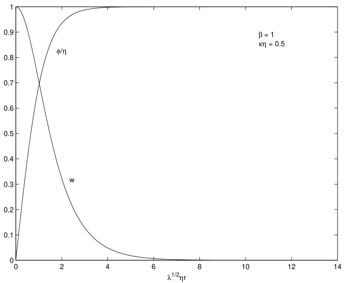
FIG. 1.: Flat-brane solutions: Scalar and gauge fields of a sub-critical monopole for $\kappa\eta=0.5$ and $\beta\equiv\lambda/e^{2}=1$. The scalar field rapidly approaches $\eta$ and the gauge field approaches zero at large $r$.

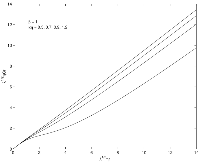
FIG. 2.: Flat-brane solutions: The metric coefficient $Cr$ of sub-critical monopoles for $\beta=1$ and $\kappa\eta=0.5,0.7,0.9,1.2$, from the top down. As $\eta$ approaches the critical value, a ‘cigar’-like region develops near the core.

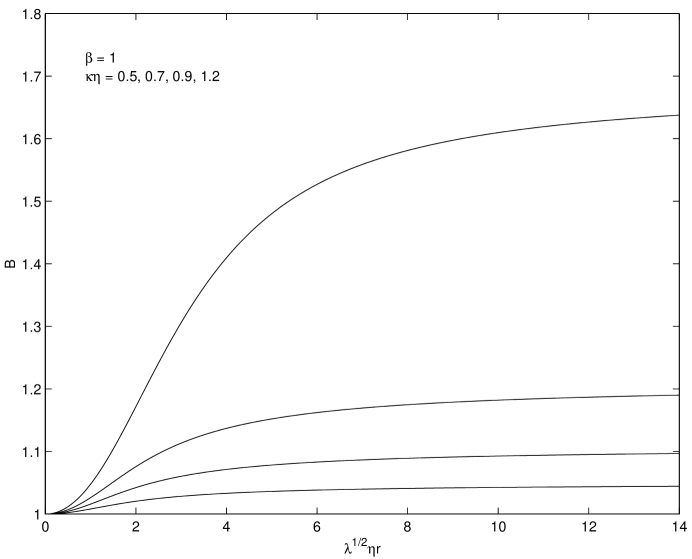
FIG. 3.: Flat-brane solutions: The metric coefficient $B$ of sub-critical monopoles for $\beta=1$ and $\kappa\eta=0.5,0.7,0.9,1.2$, from the bottom up.

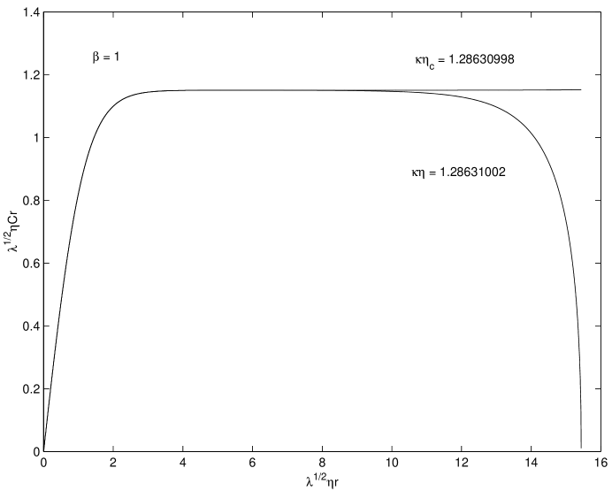
FIG. 4.: Flat-brane solutions: The metric coefficient $Cr$ of a critical monopole, $\kappa\eta_{c}=1.28630998$, and of a super-critical monopole, $\kappa\eta=1.28631002$, for $\beta=1$. For the critical monopole, $Cr$ is a constant, while for the super-critical monopole it drops to zero at the singularity.

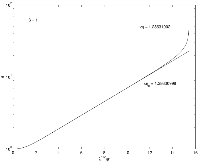
FIG. 5.: Flat-brane solutions: The metric coefficient $B$ of a critical and a super-critical monopole, for the same parameter values as in Fig. 4. For the critical monopole, $B$ is an exponential function of $r$, while for the super-critical monopole it diverges at the singularity.

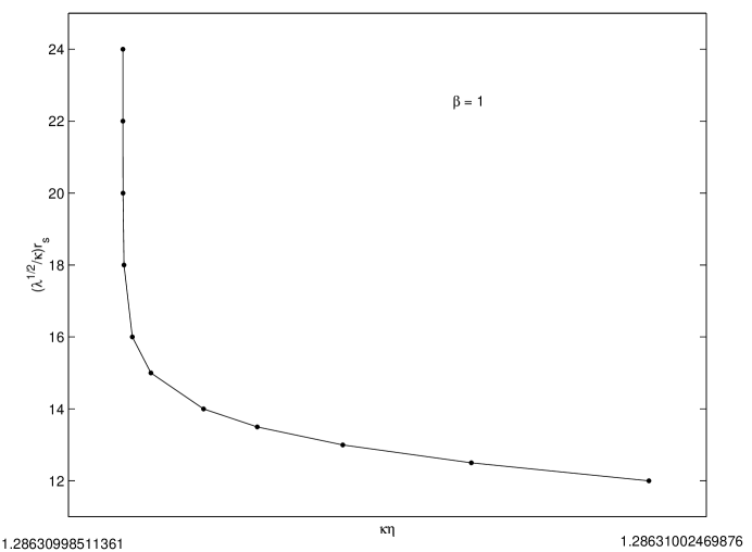
FIG. 6.: Location of the singularity $r_{s}$ vs. $\eta$ for $\beta=1$. $r_{s}$ moves away from the core as $\eta$ is decreased and becomes infinite at the critical value $\eta_{c}$.

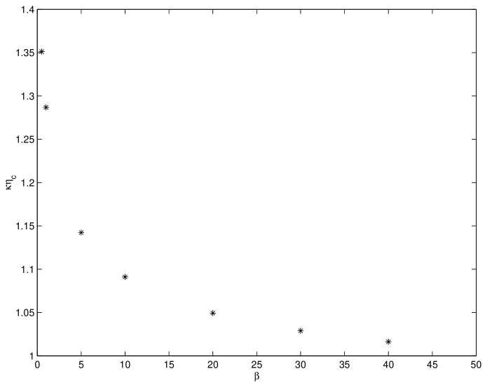
FIG. 7.: Flat-brane solutions: The critical value $\kappa\eta_{c}$ for several values of $\beta=0.5,1,5,10,20,30,40$.

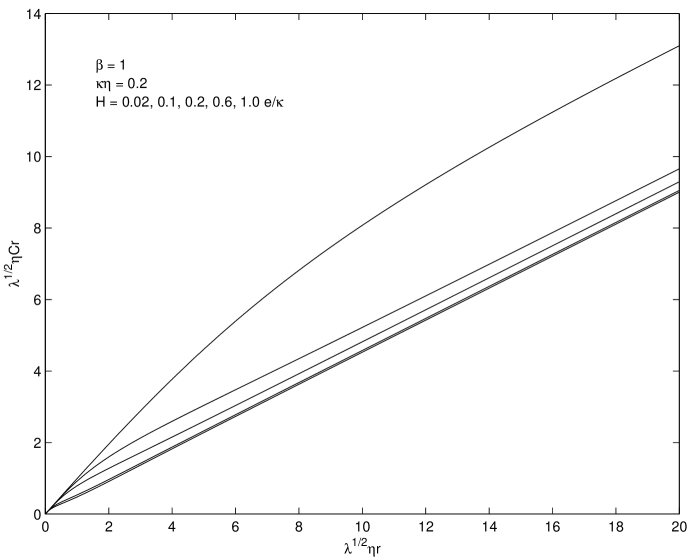
FIG. 8.: Inflating-brane solutions: The metric coefficient $Cr$ of sub-critical monopoles for $\kappa\eta=0.2$ and $\beta=1$, with the expansion rate $H=0.02,0.1,0.2,0.6,1.0e/\kappa$ from the top down.

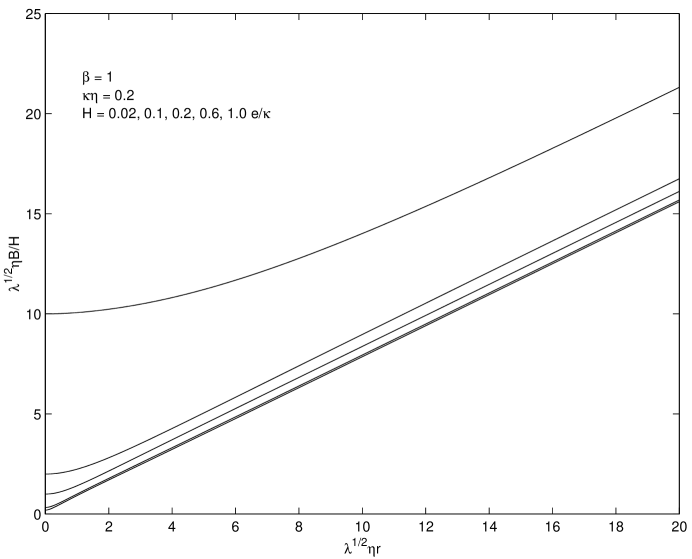
FIG. 9.: Inflating-brane solutions: The metric coefficient $B$ of sub-critical monopoles for $\kappa\eta=0.2$ and $\beta=1$, with $H=0.02,0.1,0.2,0.6,1.0e/\kappa$ from the top down.

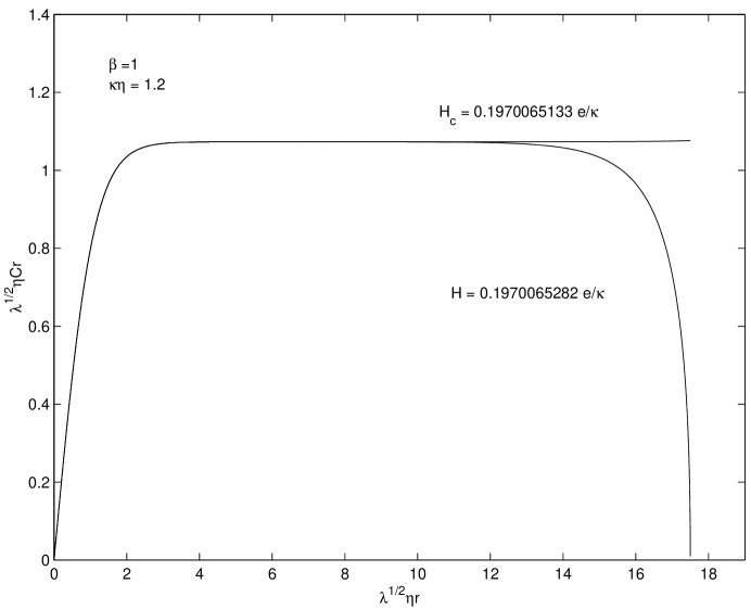
FIG. 10.: Inflating-brane solutions: The metric coefficient $Cr$ of a sub-critical monopole with $\kappa\eta=1.2<\kappa\eta_{c}$ and $\beta=1$, for two values of the expansion rate $H$: the critical rate $H_{c}=0.1970065133e/\kappa$, and a super-critical rate $H=0.1970065282e/\kappa$.

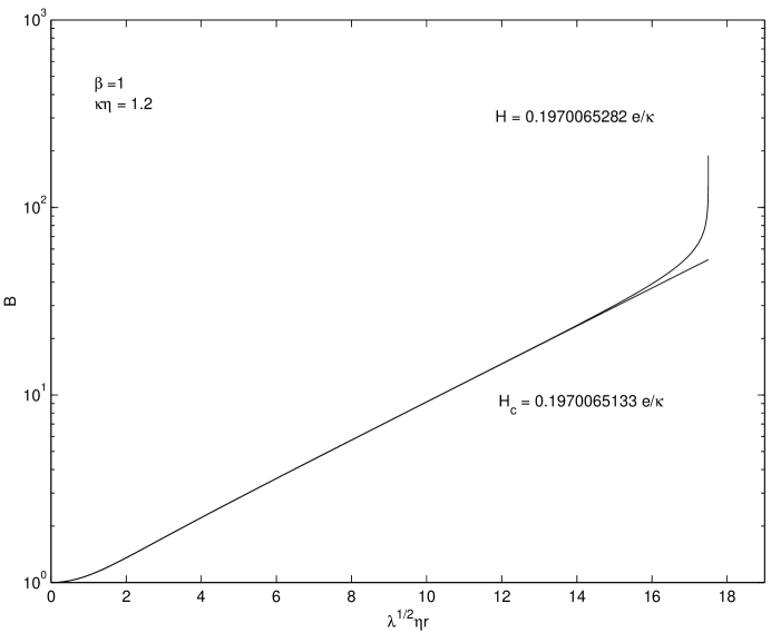
FIG. 11.: Inflating-brane solutions: The metric coefficient $B$ of a sub-critical inflating monopole, for the same parameter values as in Fig. 10.

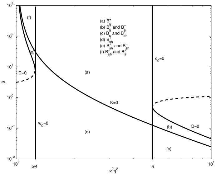
FIG. 12.: The parameter space of inflating cigar solutions.

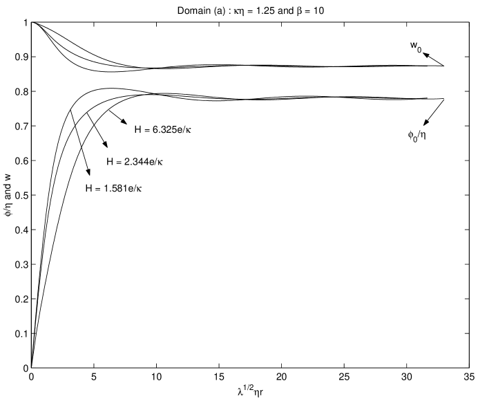
FIG. 13.: Inflating-brane solutions in domain (a): Scalar and gauge fields for $\kappa\eta=1.25$, $\beta=10$ and $H=1.581,2.344,6.325e/\kappa$.

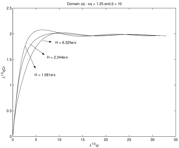
FIG. 14.: Inflating-brane solutions in domain (a): The metric coefficient $Cr$ for the same parameters as in Fig. 13.

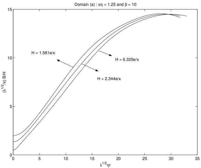
FIG. 15.: Inflating-brane solutions in domain (a): The metric coefficient $B$ for the same parameters as in Fig. 13.

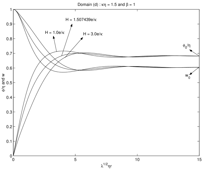
FIG. 16.: Inflating-brane solutions in domain (d): Scalar and gauge fields for $\kappa\eta=1.5$, $\beta=1$ and $H=1.0,1.507439,3.0e/\kappa$.

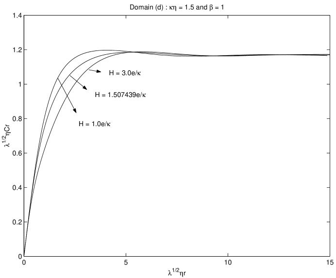
FIG. 17.: Inflating-brane solutions in domain (d): The metric coefficient $Cr$ for the same parameters as in Fig. 16.

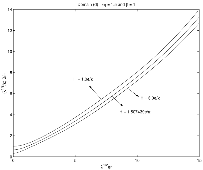
FIG. 18.: Inflating-brane solutions in domain (d): The metric coefficient $B$ for the same parameters as in Fig. 16.