Conformal Transformations of S-Matrix in Scalar Field Theory

Abstract

In this paper, three methods for describing the conformal transformations of the S-matrix in quantum field theory are proposed. They are illustrated by applying the algebraic renormalization procedure to the quantum scalar field theory, defined by the LSZ reduction mechanism in the BPHZ renormalization scheme. Central results are shown to be independent of scheme choices and derived to all orders in loop expansions. Firstly, the local Callan–Symanzik equation is constructed, in which the insertion of the trace of the energy-momentum tensor is related to the beta function and the anomalous dimension. With this result, the Ward identities for the conformal transformations of the Green functions are derived. Then the conformal transformations of the S-matrix defined by the LSZ reduction procedure are calculated. Secondly, the conformal transformations of the S-matrix in the functional formalism are related to charge constructions. The commutators between the charges and the S-matrix operator are written in a compact way to represent the conformal transformations of the S-matrix. Lastly, the massive scalar field theory with local coupling is introduced in order to control breaking of the conformal invariance further. The conformal transformations of the S-matrix with local coupling are calculated.

I Introduction

The S-matrix plays a fundamental role in quantum field theory. It is always used to construct the cross section, which can be checked by measurements of scattering experiments. On the other hand, it is also one way of defining quantum field theory. For example, in the Epstein–Glaser scheme, see epstein , the locality and the unitarity of the S-matrix with local coupling determine the whole theory. Furthermore, symmetries of the S-matrix have been studied on an abstract level coleman ; hagg .

In this paper, we study the conformal transformations of the S-matrix in four dimensional flat space-time. When the mass of particles can be neglected in high energy experiments, the theory could be regarded as conformally invariant at least in the classical approximation. Hence, solving problems of this type is helpful to simplify calculations or to find some identities in phenomenological physics. At the abstract level, it also may improve knowledge on how to control anomalies or breakings in quantum field theory.

The conformal transformations consist of the Poincaré transformations, the dilatation transformation and the special conformal transformation. In all versions of ordinary quantum field theory the S-matrix has to be Poincaré invariant, which has been verified in all experiments until now. But generally, the S-matrix is not invariant under the dilatation transformation and the special conformal transformation even if the corresponding classical theory is conformally invariant. Some research has been carried out on the breaking of the conformal invariance. For example, in the massless $\phi^{4}$ theory constructed by a nonperturbative approach in Zimmer1 , the dilatation transformation of the S-matrix is given by

$$\sum_{i=1}^{n}\left(1+p_{i}\partial_{p_{i}}\right)S_{n}=\beta_{\lambda}\partial_{\lambda}S_{n},$$ (1)

where $\gamma$, the anomalous dimension, does not contribute.

We will treat our problem in the approach of the algebraic renormalization introduced in brs1 ; brs2 , also see sibold1 ; piguet ; schweda . It is based on the quantum action principle, relating differentiation (or variation) on parameters (or fields) to local insertions Low1 ; Low2 ; Lam1 ; Lam2 . There are two guiding arguments about the quantum action principle. Firstly, it is independent of regularization schemes and renormalization procedures. Secondly, the perturbative quantum action principle is satisfied to all orders of $\hbar$. Hence they provide strong power for the algebraic renormalization procedure. Furthermore, the algebra of the global (local) Ward identity operators (or the cohomology of the Slavnov–Taylor identity operator) can be realized by the differential (variational) operators. By imposing them as constraints on local insertions, the global (local) Ward identities (or the Slavnov–Taylor identity) can be constructed to all orders in loop expansions.

The global Ward identity for the conformal transformation of the vertex functional $\Gamma[\phi]$ can be defined respectively by

$$\mathcal{W}^{i}\Gamma[\phi]:=\int\!\!{\rm d}^{4}x\,\delta^{i}\phi(x){\frac{\delta\Gamma[\phi]}{\delta\phi(x)}},\qquad\qquad i=T,L,D,K,$$ (2)

where the symbol $\mathit{T}$ denotes translation, the symbol $\mathit{L}$ denotes Lorentz rotations, the symbol $\mathit{D}$ denotes dilatation and the symbol $\mathit{K}$ denotes special conformal transformation. If we redefine the global Ward identity operator $\mathcal{W}^{i}$ by $-\mathcal{W}^{i}$, the new global Ward identity operator exactly forms a representation of the conformal algebra. The corresponding local Ward identity operator is given by

$$\mathbf{w}^{i}(x)=\delta^{i}\phi(x){\frac{\delta}{\delta\phi(x)}},\qquad\qquad i=T,L,D,K.$$ (3)

It is not unique since we can add total derivatives without changing the global Ward identity (2).

Although the approach of algebraic renormalization does not rely on the choices of renormalization schemes, we choose the BPHZ renormalization scheme in Zimmer2 to define the scalar field theory. The main reason is that in this scheme insertions can be realized by the normal product algorithm, see Low1 , Zimmer3 , Zimmer4 . Then we can directly calculate insertions in detail instead of using algebraic constraints. Furthermore, we can use the Zimmermann identities defined in the BPHZ renormalization scheme which relate insertions with different subtraction degrees, see Zimmer3 . As a matter of fact, however, the central results in the paper are independent of the scheme choices.

The S-matrix is given by amputation of external propagators of the Green function in the on-shell limit in the LSZ reduction procedure, which suggests that the breaking of the conformal invariance have to be first controlled at the level of the Green functions. Actually, they are determined by insertion of the trace of the energy-momentum tensor which is related to the local Callan–Symanzik equation. With it in hand, we can calculate the Ward identities for the conformal transformations to all orders in loop expansions. By integrating both sides, the Callan–Symanzik equation, see Callan ; Symanzik , can be obtained and directly related to the dilatation transformation. The special conformal transformation of the Green function is obtained in a similar manner. Afterwards, the conformal transformations of the S-matrix can be calculated by applying the LSZ reduction formula.

Furthermore, the LSZ reduction procedure can be used to construct the charges responsible for the conformal transformations with the local Ward identities. For example, the charges for the $\mathit{BRST}$ transformations have been obtained in Kugo1 ; Kugo2 . The commutators between the charges and the S-matrix operator are to represent the conformal transformations of the S-matrix in the functional formalism.

Moreover, we will introduce local coupling instead of the coupling constant in order to control the conformal breaking further. The massive $\phi^{4}$ model with local coupling can be constructed by means of Poincaré invariance and power counting renormalizability. The local Callan–Symanzik equation is also calculated then applied to the calculation of the conformal transformations of the S-matrix.

In addition, we try to obtain the conformal transformations of the S-matrix in the massless case. In a general sense, it does not exist due to infra-red divergence. But in Zimmer1 by imposing some necessary physical postulates, the S-matrix in the massless $\phi^{4}$ field theory can be proved to exist in a nonperturbative way. Here, we directly assume that it exists and that it can be obtained by taking the massless limit of the S-matrix defined in the massive model. Naturally, such a treatment is purely formal.

The plan of this paper is the following. In the second section, a general procedure to solve our problem is proposed. In the third section, we study the conformal transformations of the S-matrix in the massive ${\phi}^{4}~{}model$ defined by the BPHZ renormalization procedure. In the fourth section, the conformal transformations of the S-matrix are given by the commutators between the S-matrix operators and the corresponding charges. In the fifth section, the conformal transformations of the S-matrix in the massive ${\phi}^{4}~{}model$ with local coupling are calculated. In our conclusion, some remarks suggest that three methods employed in this paper are also suitable for other models such as non-abelian gauge field theories or supersymmetrical gauge field theories. In Appendix A, the proof supporting that the dilatation transformation of the S-matrix goes without on-shell poles is presented. In Appendix B, the problem whether the special conformal transformation of the S-matrix has on-shell poles or not is discussed up to two-loop order. In Appendix C, current constructions and charge constructions via the local Ward identities are presented in detail.

II The general procedure for calculating the conformal transformations of the S-Matrix

In this section, we propose the general procedure by showing an example of how to construct the dilatation transformations of the S-matrix in the massive ${\phi}^{4}~{}model$.

The S-matrix is constructed from the Green function by the amputation of its external propagators in the on-shell limit. With the LSZ reduction procedure, the S-matrix in the momentum space is given by the following expression,

$$S_{n}=\lim_{p_{i}{\in}P}(-ir^{-{\textstyle\frac{1}{2}}})^{n}\prod_{i=1}^{n}({p_{i}}^{2}-m^{2})\,G_{n}(p_{1},p_{2},\cdots,p_{n}),$$ (4)

where $S_{n}(p_{1},p_{2},\cdots,p_{n})$ is the $n$-particle scattering matrix element; $G_{n}(p_{1},p_{2},\cdots,p_{n})$ is the $n$-particle general Green function, but here we only take the connected part which contains the factor $\delta^{4}(p_{1}+p_{2}+\cdots+p_{n})$; $r$ is the wavefunction renormalization constant; $p_{i}$ is the momentum of ith particle, $m$ is the mass of the scalar particle; and $P$ is the set defined by

$$P:=\{p_{i}\mid p_{i}^{2}=m^{2};~{}{p_{i}}^{0}>0;~{}i=1,2\cdots n\}.$$ (5)

The wavefunction renormalization constant $r$ is also defined by

$${\frac{1}{r}}:=\partial_{p^{2}}\widetilde{\Gamma}_{2}{(p,-p)}\mid_{p^{2}=m^{2}},$$ (6)

where $\widetilde{\Gamma}_{2}{(p,-p)}$ is the two-point $1PI$(one particle irreducible) Green function.

The dilatation transformation of the S-matrix can be defined by

$$\mathcal{W}^{D}\,S_{n}:=\sum_{i=1}^{n}\left(1+p_{i}\partial_{p_{i}}\right)\,S_{n}(p_{1},p_{2},\cdots,p_{n}),$$ (7)

$\mathcal{W}^{D}$ being the Ward identity operator for the dilatation transformation. With the definition of the S-matrix, first, we have to control the breaking of the dilatation invariance of the Green function, namely we have to calculate

$$\mathcal{W}^{D}\,G_{n}:=\sum_{i=1}^{n}\left(1+x_{i}\partial_{x_{i}}\right)\,G_{n}(x_{1},x_{2},\cdots,x_{n}).$$ (8)

Second we shall treat the derivative of the following type,

$$\partial_{p_{i}}\left\{f(p_{1},\cdots,p_{n})\mid_{P}\right\},$$ (9)

since the S-matrix is obtained by taking the on-shell limit. It is observed that there is no direct access to the derivative (9), because in the general case we have

$$\partial_{p_{i}}\left\{f(p_{1},\cdots,p_{n})\mid_{P}\right\}\neq\partial_{p_{i}}f(p_{1},\cdots,p_{n})\mid_{P}.$$ (10)

The derivative $p_{i}\partial_{p_{i}}\left\{f(p_{1},\cdots,p_{n})\mid_{P}\right\}$ is not well-defined since the on-shell condition $p_{i}^{2}$$=$$m^{2}$ means that $p_{i}^{0}$, $p_{i}^{1}$, $p_{i}^{2}$, $p_{i}^{3}$ are not independent of each other, but $\partial_{p_{i}}f(p_{1},\cdots,p_{n})\mid_{P}$ is well-defined and hence can be used to define the previous one.

Introducing two new functions,

$$G_{A,n} := \,(ir^{-{\textstyle\frac{1}{2}}})^{n}\prod_{i=1}^{n}(\Box_{x_{i}}+m^{2})\,G_{n}(x_{1},x_{2},\cdots,x_{n}),$$ (11)

$$S_{A,n} := \,\int\!\prod_{i=1}^{n}{\rm d}^{4}x_{i}\,\,e^{i\sum_{j=1}^{n}{p_{j}\cdot x_{j}}}\,G_{A,n},$$ (12)

the S-matrix element $S_{n}$ is obtained to be found to be

$$S_{n}=\lim_{p_{i}{\in}P}\,S_{A,n}(p_{1},p_{2},\cdots,p_{n}),$$ (13)

which implies that we can construct $\mathcal{W}^{D}\,S_{n}$ with ${\mathcal{W}}^{D}S_{A,n}\mid_{P}$. Hence it is necessary to understand what ${\mathcal{W}}^{D}S_{A,n}\mid_{P}$ does mean in a physical sense.

Furthermore, for convenience, we introduce the notation ${\mathcal{F}}^{A}_{n}(x;p)$ to denote the action of both the Fourier transformation and the amputation, namely

$${\mathcal{F}}^{A}_{n}(x;p):=(ir^{-{\textstyle\frac{1}{2}}})^{n}\int\!\!\prod_{i=1}^{n}{\rm d}^{4}x_{i}\,\,e^{i\sum_{j=1}^{n}{p_{j}\cdot x_{j}}}\,\prod_{i=1}^{n}(\Box_{x_{i}}+m^{2}),$$ (14)

where $(x;p)$ is the abbreviation of $(x_{1},\cdots x_{n};p_{1},\cdots p_{n})$. Then $S_{A,n}$ is denoted by ${\mathcal{F}}^{A}_{n}(x;p)G_{n}$. We also introduce the notation ${\mathcal{F}}^{A}_{n}(x,\check{x}_{l};p)$:

$${\mathcal{F}}^{A}_{n}(x,\check{x}_{l};p):=(ir^{-{\textstyle\frac{1}{2}}})^{n}\int\!\!\prod_{i=1}^{n}{\rm d}^{4}x_{i}\,\,e^{i\sum_{j=1}^{n}{p_{j}\cdot x_{j}}}\,\prod_{i=1,i\neq l}^{n}(\Box_{x_{i}}+m^{2}).$$ (15)

Similarly, ${\mathcal{F}}^{A}_{n}(x;-q)$ and ${\mathcal{F}}^{A}_{n}(x,\check{x}_{l};-q)$ are given by replacing the momentum $p_{i}$ with $-q_{i}$ in the corresponding parts.

The general procedure for calculating the conformal transformations of the S-matrix can be concluded as follows. As a starting point, we must have a set of well-defined Green functions. Then we carry out the following steps.

1. Calculate $\mathcal{W}^{D}\,G_{n}(x_{1},x_{2},\cdots,x_{n})$;

2. Calculate $\mathcal{W}^{D}\,G_{A,n}(x_{1},x_{2},\cdots,x_{n})$;

3. Calculate $\mathcal{W}^{D}\,S_{A,n}(p_{1},p_{2},\cdots,p_{n})$;

4. Calculate $\mathcal{W}^{D}\,S_{n}(p_{1},p_{2},\cdots,p_{n})$.

In order to check the result, we can compare $\mathcal{W}^{D}\,S_{n}(p_{1},p_{2},\cdots,p_{n})$ with known results in case they exist. If we can control the breaking further, then we have to repeat all the above steps. Moreover, there are several reasons for introducing the above procedure. First of all, they are set up for solving the puzzle of how to define the derivation on the on-shell objects. Second, carrying out them step by step will be helpful to choose suitable formalisms of the conformal transformations as realizations of differential operators. Third, like what we will do in the fourth section, the conformal transformations of the S-matrix can be also calculated by the commutators between charges and the S-matrix operator. However, as will be shown, to define charges for the conformal transformations is not an easy task.

III Conformal transformations of the S-matrix
in the massive scalar model

A well-defined perturbative quantum field theory provides at least exact rules to compute renormalized Green functions and derive relations among different renormalized Green functions. In this section, the conformal transformations of the S-matrix in the well-defined massive ${\phi}^{4}~{}model$ will be calculated. The massive ${\phi}^{4}~{}model$ will be defined in the BPHZ renormalization scheme where the insertions of the composite operators are represented by normal products in Zimmer2 . However, most results can be also obtained from other regularization schemes or renormalization procedures.

III.1 The massive ${\phi}^{4}~{}model$ via the BPHZ renormalization procedure

In this subsection, the well-defined massive ${\phi}^{4}~{}model$ in the BPHZ renormalization scheme is introduced. Namely, the renormalized action, the renormalization conditions, the Zimmermann’s forest formula, the renormalized Green function, the renormalized Green function with the insertions of the normal products, the quantum action principle and the Zimmermann identities are presented.

The renormalized action $\Gamma_{\rm ren}$ can be regarded as the sum of the free part $\Gamma_{0}$ and the interaction part $\Gamma_{\rm int}$,

$$\Gamma_{\rm ren}=\Gamma_{0}+\Gamma_{\rm int}=-z\,{\Delta}_{1}-\,a{\Delta}_{2}-{\rho}\,{\Delta}_{4}.$$ (16)

In the tree approximation, the coefficients $z$, $a$, $\rho$ are specified by

$$z^{(0)}=1,\qquad a^{(0)}=m^{2},\qquad\rho^{(0)}=\lambda,$$ (17)

where the upper indices denote the power counting of $\hbar$ in this section. The normal products ${\Delta}_{1}$, ${\Delta}_{2}$, ${\Delta}_{4}$ are given by

$${\Delta}_{1} = \left[\int\!\!{\rm d}^{4}x\,{\textstyle\frac{1}{2}}\phi(x)\Box\phi(x)\right]_{4},$$ (18)

$${\Delta}_{2} = \left[\int\!\!{\rm d}^{4}x\,{\textstyle\frac{1}{2}}\phi^{2}(x)\right]_{4},$$ (19)

$${\Delta}_{4} = \left[\int\!\!{\rm d}^{4}x\,{\frac{1}{4!}}{\phi^{4}(x)}\right]_{4}.$$ (20)

The free part $\Gamma_{0}$ is given by $-{\Delta}_{1}-m^{2}{\Delta}_{2}$ determining the propagator. The renormalized Lagrangian density is chosen to be

$$\mathcal{L}_{\rm ren}=-{\textstyle\frac{1}{2}}\,z\,\phi\Box\phi-\,{\textstyle\frac{1}{2}}\,a\phi^{2}-{\frac{1}{4!}}\rho\phi^{4},$$ (21)

but it can be changed by adding total derivatives. On the other hand, the renormalized action $\Gamma_{\rm ren}$ is also the sum of the classical action $\Gamma_{\rm cl}$ and all the possible local counterterms $\Gamma_{\rm counter}$, namely

$$\Gamma_{\rm ren}=\Gamma_{\rm cl}+\Gamma_{\rm counter}=-\int({\textstyle\frac{1}{2}}\,\phi(\Box+m^{2})\phi+{\frac{1}{4!}}\lambda\phi^{4})+\mathcal{O}(\hbar).$$ (22)

In higher orders, the coefficients $z$, $a$, $\rho$ are decided by the renormalization conditions

$$\widetilde{\Gamma}_{2}{(p,-p)}\mid_{p^{2}=m^{2}} = 0,$$ (23)

$$\partial_{p^{2}}\widetilde{\Gamma}_{2}{(p,-p)}\mid_{p^{2}={\mu}^{2}} = 1,$$ (24)

$$\widetilde{\Gamma}_{4}{(p_{1},p_{2},p_{3},p_{4})}\mid_{Q} = -\lambda,$$ (25)

where $m$ is the physical mass, $\mu$ is the normalization mass denoting the renormalization scale, $\lambda$ is the physical coupling constant and $Q$ is the set given by

$$Q={\{p_{i}\mid p_{i}^{2}={\mu}^{2},(p_{i}+p_{j})^{2}={\frac{4}{3}}{\mu}^{2};i\neq j;i,j=1,2,3,4\}}.$$ (26)

$\widetilde{\Gamma}_{2}{(p,-p)}$ and $\widetilde{\Gamma}_{4}{(p_{1},p_{2},p_{3},p_{4})}$ are the two-point $1PI$ Green function and the four-point $1PI$ Green function respectively. Here the rule of the Fourier transformation of an ordinary function, such as the Green function or 1PI Green function, between the momentum space and the coordinate space has been chosen as

$$F(p_{1},p_{2},\cdots,p_{n}) = (2\,\pi)^{4}\,\delta^{4}\left(\sum_{i=1}^{n}\,p_{i}\right)\,\widetilde{F}(p_{1},p_{2},\cdots,p_{n})$$ (27)

$$= \int\!\!\prod_{i=1}^{n}{\rm d}^{4}x_{i}\,\,e^{i\sum_{j=1}^{n}{p_{j}\cdot x_{j}}}\,\,F(x_{1},x_{2},\cdots,x_{n}).$$

The Zimmermann forest formula was given in Zimmer2 . It denotes a procedure for obtaining the renormalized Feynman integrand $R_{\Gamma}(p,k)$ from the unrenormalized Feynman integrand $I_{\Gamma}(p,k)$, namely

$$R_{\Gamma}(p,k)=\sum_{U\in{\mathcal{F}}}\,S_{\Gamma}\prod_{\gamma\in U}\,(-t^{\delta_{\gamma}}S_{\gamma})\,\,I_{\Gamma}(p,k),$$ (28)

where $U$ is a forest, ${\mathcal{F}}$ is a set of all possible renormalization forests, $S_{\Gamma}$ or $S_{\gamma}$ are substitution operators, $t^{\delta_{\gamma}}$ is the Taylor subtraction operator cut off by the subtraction degree $\delta_{\gamma}$, the argument $p$ denotes a set of external momenta and the argument $k$ denotes a set of independent internal momenta.

The renormalized Green function in the BPHZ renormalization procedure was defined in Zimmer3 ; Zimmer4 . The unrenormalized Green function is given in the Gell-Mann$-$Low formulation and its renormalized version is directly defined as the finite part under the BPHZ renormalization procedure,

$$\langle T\phi(x_{1})\phi(x_{2})\cdots\phi(x_{n})\rangle$$

$$:={BPHZ}~{}\mbox{finite part ~{}of~{}}$$

$$\langle T\phi_{0}(x_{1})\phi_{0}(x_{2})\cdots\phi_{0}(x_{n})e^{{\frac{i}{\hslash}}{\Gamma}^{0}_{\rm int}}\rangle/\langle Te^{{\frac{i}{\hslash}}{\Gamma}^{0}_{\rm int}}\rangle.$$ (29)

The renormalized Green function with insertions of normal products is given by

$$\prod_{i}N_{\delta_{i}}\left[Q_{i}(y_{i})\right]\cdot G_{n}(x_{1},x_{2},\cdots,x_{n})$$ (30)

$$:= \langle T\prod_{i}N_{\delta_{i}}\left[Q_{i}(y_{i})\right]\phi(x_{1})\phi(x_{2})\cdots\phi(x_{n})\rangle$$

$$= {BPHZ}~{}\mbox{finite part ~{}of~{}}$$

$$\langle T\prod_{i}N_{\delta_{i}}\left[Q^{0}_{i}(y_{i})\right]\phi_{0}(x_{1})\phi_{0}(x_{2})\cdots\phi_{0}(x_{n})e^{{\frac{i}{\hslash}}{\Gamma}^{0}_{\rm int}}\rangle/\langle Te^{{\frac{i}{\hslash}}{\Gamma}^{0}_{\rm int}}\rangle,$$

where the normal products $N_{\delta_{i}}\left[Q^{0}_{i}(y_{i})\right]$ denote vertices to be treated with the subtraction degree $\delta_{i}$. The symbols with the upper index $0$ are defined in free quantum field theory. For convenience, the subtraction degrees of normal products will not be explicitly given in some cases.

The quantum action principle was derived in the BPHZ renormalization procedure, see Low1 ; Low2 ; Lam1 ; Lam2 . It means that variations of parameters or fields of the Green function can be represented by appropriate local insertions. Its differential formalism is given in the following way,

$$\partial_{A}\Gamma = \left[\partial_{A}\Gamma_{\rm ren}\right]_{4}\cdot\Gamma,~{}~{}~{}~{}~{}A=m,{\mu},\lambda,$$ (31)

$${\phi(x){\frac{\delta\Gamma}{\delta\phi(x)}}} = \left[\phi(x){\frac{\delta\Gamma_{\rm ren}}{\delta\phi(x)}}\right]_{4}\cdot\Gamma,$$ (32)

where the lower indices of normal products are the subtraction degrees used in the BPHZ renormalization scheme.

The Zimmermann identities were proved in Zimmer3 ; Zimmer4 . They relate the subtraction and the over-subtraction in the BPHZ renormalization procedure. They are given by

$$N_{\delta}\left[Q\right]\cdot\Gamma=\sum_{i}u_{i}N_{\chi}\left[Q_{i}\right]\cdot\Gamma,$$ (33)

where the sum is over all possible normal products of the over-subtraction degree $\chi$ with same quantum numbers, and $\delta$ is the subtraction degree, with $\chi$$>$$\delta$. The coefficients $u_{i}$ are determined by normalization conditions on insertions of composite operators.

III.2 The local Callan–Symanzik equation

First of all, we have to control the breaking of the conformal invariance of the Green function. Choosing one suitable momentum construction of the local Ward identity operator for the translation transformation as

$$\widetilde{\mathbf{w}}_{\mu}^{T}(x)=\partial_{\mu}\phi(x){\frac{\delta}{\delta\phi(x)}}-{\frac{1}{4}}\partial_{\mu}\left(\phi(x){\frac{\delta}{\delta\phi(x)}}\right),$$ (34)

the breaking of the conformal invariance will be determined by the insertion of the trace of the energy-momentum tensor $T_{\mu\nu}$ given by

$$T_{\mu\nu}=z\partial_{\mu}\phi\partial_{\nu}\phi-\eta_{\mu\nu}({\frac{1}{2}}z\partial\phi\partial\phi+{\frac{1}{4}}z\phi\Box\phi-{\frac{1}{4}}a\phi^{2})-c(\partial_{\mu}\partial_{\nu}-\eta_{\mu\nu}\Box)\phi^{2},$$ (35)

where $T_{\mu\nu}$ satisfies $\widetilde{\mathbf{w}}_{\mu}^{T}(x)\Gamma_{\rm ren}=-\partial^{\nu}[T_{\mu\nu}(x)]_{4}$, $\eta_{\mu\nu}$ is a metric given in Minkowski space-time and $c$ is a constant determined by coupling the energy-momentum tensor $T_{\mu\nu}$ to a curved background, see elisabeth1 ; elisabeth2 .

The dilatation transformation of the vertex functional $\Gamma$ is defined by

$$\mathcal{W}^{D}\Gamma[\phi] := \int\!\!{\rm d}^{4}x\,(1+x\partial_{x})\phi(x)\,{\frac{\delta\Gamma[\phi]}{\delta\phi(x)}}$$ (36)

$$= \int\!\!{\rm d}^{4}x\,[T^{\nu}_{\nu}]_{4}\cdot\Gamma.$$

The special conformal transformation of the vertex functional $\Gamma$ is defined by

$$\alpha\mathcal{W}^{K}\Gamma[\phi] := \int\!\!{\rm d}^{4}x\,\left(\alpha^{\nu}(2x_{\nu}x^{\mu}-\eta^{\mu}_{\nu}x^{2})\partial_{\mu}+2\alpha x\right)\phi(x)\,{\frac{\delta\Gamma[\phi]}{\delta\phi(x)}}$$ (37)

$$= \int\!\!{\rm d}^{4}x\,\,(2\alpha x)\,[T^{\nu}_{\nu}]_{4}\cdot\Gamma,$$

where the symbol $\alpha$ is a constant parameter and $\alpha\mathcal{W}^{K}$ denotes the scalar product of $\alpha^{\nu}\mathcal{W}^{K}_{\nu}$.

Hence we have to first carry out the insertion of the trace of the energy-momentum tensor into the vertex functional $\Gamma$. With the known $\beta_{\lambda}$ function and the anomalous dimension $\gamma$ used in the Callan–Symanzik equation, the local Callan–Symanzik equation is obtained by

$$-[T^{\nu}_{\nu}]_{4}\cdot\Gamma+\beta_{\lambda}[\partial_{\lambda}\mathcal{L}_{\rm ren}]_{4}\cdot\Gamma-{\textstyle\frac{1}{2}}\gamma\phi{\frac{\delta}{\delta\phi}}\Gamma$$

$$=(z-6c-{\textstyle\frac{1}{2}}\alpha_{m}s)[\phi\Box\phi+\partial\phi\partial\phi]_{4}\cdot\Gamma+{\textstyle\frac{1}{2}}\alpha_{m}[\phi^{2}]_{2}\cdot\Gamma,$$ (38)

where $\alpha_{m}$ is a parameter to be determined, and we have used the Zimmermann identity given by

$${\textstyle\frac{1}{2}}[\phi^{2}]_{2}\cdot\Gamma={\textstyle\frac{1}{2}}[\phi^{2}]_{4}\cdot\Gamma+{\textstyle\frac{1}{2}}s\,[\partial\phi\partial\phi]_{4}\cdot\Gamma+{\textstyle\frac{1}{2}}r\,[\phi\Box\phi]_{4}\cdot\Gamma+{\frac{1}{4!}}t\,[\phi^{4}]_{4}\cdot\Gamma,$$ (39)

the parameters $s$, $r$, $t$ being fixed by the normalization conditions on the insertions of the related composite operators. By defining $\alpha_{m}$, $\beta_{\lambda}$ and $\gamma$ as the solutions of the following three equations:

$$\left\{\begin{array}[]{lll}\alpha_{m}&=&-2a-\beta_{\lambda}\partial_{\lambda}a+\gamma a,\\ {\alpha_{m}}(r-s)&=&-\beta_{\lambda}\partial_{\lambda}z+\gamma z,\\ {\alpha_{m}}t&=&-\beta_{\lambda}\partial_{\lambda}\rho+2\gamma\rho,\end{array}\right.$$ (40)

we arrive at the conventional form of the Callan–Symanzik equation.

The Callan–Symanzik equation like the ordinary one can be obtained by integrating the both sides of the equation (III.2),

$$\left(m\partial_{m}+\beta_{\lambda}\partial_{\lambda}-{\textstyle\frac{1}{2}}\gamma{\mathcal{N}}\right)\Gamma=\alpha_{m}\,{\Delta}_{d}\cdot\Gamma,$$ (41)

where the symbol $m\partial_{m}$ denotes $m\partial_{m}+\mu\partial_{\mu}$, the classical approximation of $\alpha_{m}$ is given by $\alpha_{m}^{(0)}$$=$$-2m^{2}$ and ${\mathcal{N}}$ and the ${\Delta}_{d}$ are denoted by

$${\mathcal{N}}=\int\!\!{\rm d}^{4}x\,\phi(x){\frac{\delta}{\delta\phi(x)}},\qquad{\Delta}_{d}=\left[\int\!\!{\rm d}^{4}x\,{\textstyle\frac{1}{2}}\phi^{2}(x)\right]_{2},$$ (42)

respectively.

Three remarks are given in order. First, there are four differential operators,

$$m\partial_{m},\,\,\mu\partial_{\mu},\,\,\beta_{\lambda}\partial_{\lambda},\,\,{\mathcal{N}},$$ (43)

and one identity, the Zimmermann identity, but we only have three independent integral insertions. So, we have to obtain two constraint equations. One is just the ${Callan--Symanzik}$ equation and the other is the renormalization group equation. Second, although here the ${Callan--Symanzik}$ equation is derived in the BPHZ scheme, its formulation (41) is ordinary, independent of used schemes. Third, taking the massless limit in a formal sense, we have $\alpha_{m}$$\to$ $0$ due to

$$\alpha_{m}=-2m^{2}\,{\frac{1}{r\,\Delta_{d}\cdot\widetilde{\Gamma}_{2}|_{p^{2}=m^{2}}}}$$ (44)

as explained in Appendix A.

III.3 The Poincaré transformation of the S-matrix

The Poincaré transformations consist of translations and Lorentz rotations. That the S-matrix is invariant under Poincaré transformations is one fundamental physical requirement in axiomatic quantum field theory. We have to realize it in our approach.

The global Ward identity for space-time translations in the generating functional $Z[J]$ is defined by

$$\mathcal{W}^{T}_{\mu}\mathit{Z}[J]:=\int\!\!{\rm d}^{4}x\,J(x)\,\partial_{\mu}\,{\frac{\delta\mathit{Z}[J]}{\delta J(x)}}.$$ (45)

Similarly, the global Ward identity for Lorentz transformations is defined by

$$\mathcal{W}^{L}_{\mu\nu}\mathit{Z}[J]:=\int\!\!{\rm d}^{4}x\,J(x)\,(x_{\mu}\partial_{\nu}-x_{\nu}\partial_{\mu})\,{\frac{\delta Z[J]}{\delta J(x)}}.$$ (46)

Since the renormalized action $\Gamma_{\rm ren}$ is invariant under space-time translations and Lorentz rotations, applying the quantum action principle, we obtain

$$\mathcal{W}^{T}_{\mu}G_{n}(x_{1},x_{2},\cdots,x_{n})=0,\qquad\mathcal{W}^{L}_{\mu\nu}G_{n}(x_{1},x_{2},\cdots,x_{n})=0.$$ (47)

Due to the commutativity between the Klein-Gordon operator $\Box_{x}+m^{2}$ and the differential operators $\partial_{\mu}$ or $x_{\mu}\partial_{\nu}-x_{\nu}\partial_{\mu}$, we have

$$\mathcal{W}^{T}_{\mu}G_{A,n}(x_{1},x_{2},\cdots,x_{n})=0,\qquad\mathcal{W}^{L}_{\mu\nu}G_{A,n}(x_{1},x_{2},\cdots,x_{n})=0,$$ (48)

which are transformed into the the momentum space formulation by

$$\mathcal{W}^{T}_{\mu}S_{A,n}:=\sum_{l=1}^{n}p_{l,\mu}S_{A,n}=0,\qquad\mathcal{W}^{L}_{\mu\nu}S_{A,n}:=\sum_{l=1}^{n}\left(p_{l,\mu}{\frac{\partial}{\partial{p_{l,\nu}}}}-p_{l,\nu}{\frac{\partial}{\partial{p_{l,\mu}}}}\right)S_{A,n}=0.$$ (49)

From theses equations, we can derive the conservation of four-momentum and the fact that $S_{A,n}$ is Lorentz invariant. Then we assign to $S_{A,n}$ and $S_{n}$ two new Lorentz invariant functions $S^{\prime}_{A,n}$ and $S^{\prime}_{n}$ in the following way:

$$S_{A,n}=\delta^{4}(\sum_{i=1}^{n}\,p_{i})S^{\prime}_{A,n}(p_{i}^{2},p_{i}\cdot p_{j},m^{2}),\qquad S_{n}=\delta^{4}(\sum_{i=1}^{n}\,p_{i})S^{\prime}_{n}(p_{i}\cdot p_{j},m^{2}),$$ (50)

where the second one implies that the S-matrix is Poincaré invariant, namely,

$$\mathcal{W}^{T}_{\mu}S_{n}=0,\qquad\mathcal{W}^{L}_{\mu\nu}S_{n}=0.$$ (51)

Furthermore, we define $\sum_{i=1}^{n}\,p_{i}\partial_{p_{i}}\,S_{n}$ by

$$\sum_{i=1}^{n}\,p_{i}\partial_{p_{i}}\,S_{n}:=\sum_{i=1}^{n}\,p_{i}\partial_{p_{i}}\,S_{A,n}|_{P}-2m^{2}\delta^{4}(\sum_{i=1}^{n}\,p_{i})\sum_{i=1}^{n}\,\partial_{p_{i}^{2}}\,S^{\prime}_{A,n}|_{P},$$ (52)

$p_{i}^{2}$ and $p_{i}\cdot p_{j}$, $i\neq j$, being regarded as independent variables before the on-shell limit. When we formally take the massless limit in our approach, we find

$$\sum_{i=1}^{n}\,(1+p_{i}\partial_{p_{i}})\,S_{n}=\sum_{i=1}^{n}\,(1+p_{i}\partial_{p_{i}})\,S_{A,n}|_{P}.$$ (53)

III.4 The dilatation transformation of the S-matrix

In this subsection, the dilatation transformation of the S-matrix will be treated with the general procedure proposed above. It is well known that the breaking of the dilatational invariance can be characterized by the beta function $\beta_{\lambda}$ and the anomalous dimension $\gamma$ in the Callan–Symanzik equation. We will read off our result in the massless limit and compare it with Zimmermann’s result in Zimmer2 .

Define the global Ward identity for the dilatation transformation of the generating functional $Z[J]$ by

$$\mathcal{W}^{D}\mathit{Z}[J]:=\int\!\!{\rm d}^{4}x\,J(x)\,(1+x\partial_{x})\,{\frac{\delta\mathit{Z}[J]}{\delta J(x)}},$$ (54)

then the transformation of the general Green function $G_{n}$ under dilatation is

$$\mathcal{W}^{D}\,G_{n}=\sum_{i=1}^{n}\left(1+x_{i}\partial_{x_{i}}\right)\,G_{n}(x_{1},x_{2},\cdots,x_{n}).$$ (55)

By the dimensional analysis, the dilatation transformation of the Green function is represented by

$$\mathcal{W}^{D}\,G_{n}=m\partial_{m}\,G_{n}(x_{1},x_{2},\cdots,x_{n}),$$ (56)

where we denote ${m}{\partial}_{m}+{\mu}{\partial}_{\mu}$ by $m\partial_{m}$ for convenience.

With the Callan–Symanzik equation realized in the Green function obtained by applying the Legendre transformation to the equation (41), the dilatation transformation of the n-point Green function is obtained as

$$\mathcal{W}^{D}\,G_{n}={\frac{i}{\hbar}}\alpha_{m}{\Delta}_{d}\cdot G_{n}-(\beta_{\lambda}\partial_{\lambda}+{\textstyle\frac{1}{2}}\,n\gamma)\,G_{n},$$ (57)

where the insertion $\alpha_{m}{\Delta}_{d}\cdot G_{n}$ vanishes in the limit of large momenta due to the Weinberg asymptotic theorem wein and is thus called “soft” breaking of the dilatation invariance.

Calculating $\mathcal{W}^{D}\,G_{A,n}$, we obtain

$$\mathcal{W}^{D}\,G_{A,n} := \sum_{i=1}^{n}\left(1+x_{i}\partial_{x_{i}}\right){(ir^{-1/2})}^{n}\prod_{i=1}^{n}(\Box_{x_{i}}+m^{2})\,G_{n}$$ (58)

$$= {(ir^{-1/2})}^{n}\prod_{i=1}^{n}(\Box_{x_{i}}+m^{2})\mathcal{W}^{D}\,G_{n}$$

$$-{(ir^{-1/2})}^{n}\sum_{l=1}^{n}2\Box_{x_{l}}\prod_{i=1,i\neq l}^{n}(\Box_{x_{i}}+m^{2})\,G_{n},$$

where we used the commutator $\left[1+x\partial_{x},\Box_{x}+m^{2}\right]=-2\Box_{x}$ implying that the amputation does not commute with the dilatation transformation.

Replacing $\mathcal{W}^{D}\,G_{n}$ in the above expression with (57), we have

$$\mathcal{W}^{D}\,G_{A,n}=-\beta_{\lambda}\,\partial_{\lambda}\,G_{A,n}-{\textstyle\frac{1}{2}}n(\beta_{\lambda}\partial_{\lambda}\ln{r}+\gamma)\,G_{A,n}-2n\,G_{A,n}+{\Delta}^{\prime}_{d}\cdot G_{A,n},$$ (59)

where ${\Delta}^{\prime}_{d}\cdot G_{A,n}$ is given by

$${\Delta}^{\prime}_{d}\cdot G_{A,n}={(ir^{-1/2})}^{n}\sum_{l=1}^{n}\,2m^{2}\prod_{i=1,i\neq l}^{n}(\Box_{x_{i}}+m^{2})\,G_{n}$$

$$+(ir^{-1/2})^{n}{\frac{i}{\hbar}}\alpha_{m}\prod_{i=1}^{n}(\Box_{x_{i}}+m^{2}){\Delta}_{d}\cdot G_{n}.$$ (60)

Then the dilatation transformation of $S_{A,n}$ is given by

$$\mathcal{W}^{D}\,S_{A,n} := \sum_{i=1}^{n}\left(1+p_{i}\partial_{p_{i}}\right)S_{A,n}=-m\partial_{m}\,S_{A,n}$$ (61)

$$= \beta_{\lambda}\,\partial_{\lambda}\,S_{A,n}+{\textstyle\frac{1}{2}}n(\beta_{\lambda}\partial_{\lambda}\ln{r}+\gamma)S_{A,n}-{\Delta}^{\prime}_{d}\cdot S_{A,n},$$

where ${\Delta}^{\prime}_{d}\cdot S_{A,n}$ is the $Fourier$ transformation of ${\Delta}^{\prime}_{d}\cdot G_{A,n}$, namely

$${\Delta}^{\prime}_{d}\cdot S_{A,n}=\int\!\!\prod_{i=1}^{n}{\rm d}^{4}x_{i}\,\,e^{i\sum_{j=1}^{n}{p_{j}\cdot x_{j}}}\,{\Delta}^{\prime}_{d}\cdot G_{A,n}.$$ (62)

Taking the on-shell limit, we obtain ${\Delta}^{\prime}_{d}\cdot S_{n}$ by

$${\Delta}^{\prime}_{d}\cdot S_{n}={\Delta}^{\prime}_{d}\cdot S_{A,n}\mid_{P}.$$ (63)

Two remarks are in order. In the on-shell limit, it seems that ${\Delta}^{\prime}_{d}\cdot S_{n}$ is not a well-defined object. We have to prove that in ${\Delta}^{\prime}_{d}\cdot S_{n}$, all on-shell poles like ${\frac{1}{p_{i}^{2}-m^{2}}}$ cancel. In fact, ${\Delta}^{\prime}_{d}\cdot S_{n}$ does not include contributions from the insertion of the local integral $\Delta_{d}$ into external propagators of the Green function $G_{n}$, which makes the upper index $\prime$ meaningful,

$${\Delta}^{\prime}_{d}\cdot S_{n}={\frac{i}{\hbar}}\alpha_{m}\lim_{p_{i}\in P}{\mathcal{F}}^{A}_{n}(x;p){\Delta}_{d}^{\prime}\cdot G_{n},$$ (64)

and hence the amputation of external propagators in ${\Delta}^{\prime}_{d}\cdot S_{n}$ can be well-defined. The proof is given in Appendix A. Here, we generalize the notation ${\Delta}\cdot S_{n}$ to arbitrary insertions such as a double insertion like $\Delta_{1}\cdot\Delta_{2}$,

$$\Delta_{1}\cdot\Delta_{2}\cdot S_{A,n}:={\mathcal{F}}^{A}_{n}(x;p)\Delta_{1}\cdot\Delta_{2}\cdot G_{n}.$$ (65)

Second, the term $\beta_{\lambda}\partial_{\lambda}\ln{r}+\gamma$ can be represented by the on-shell normalization conditions. Combining the ${Callan--Symanzik}$ equation for the two-point $1PI$ Green function with dimensional analysis, we obtain a very useful equation,

$$2(1-p^{2}\partial_{p^{2}})\widetilde{\Gamma}_{2}{(p,-p)}+(\beta_{\lambda}\partial_{\lambda}-\gamma)\widetilde{\Gamma}_{2}{(p,-p)}=\alpha_{m}{\Delta}_{d}\cdot\widetilde{\Gamma}_{2}{(p,-p)}.$$ (66)

By multiplying the derivative $p^{2}\partial_{p^{2}}$ on both sides and taking the on-shell limit, we have

$$(\beta_{\lambda}\partial_{\lambda}\ln{r}+\gamma)=-2\,r\,m^{2}\partial_{p^{2}}\partial_{p^{2}}\widetilde{\Gamma}_{2}{(p,-p)}\mid_{p^{2}=m^{2}}$$

$$-\alpha_{m}\,r\partial_{p^{2}}{\Delta}_{d}\cdot\widetilde{\Gamma}_{2}{(p,-p)}\mid_{p^{2}=m^{2}}.$$ (67)

With the following dimensional analysis:

$$\left(\sum_{j=1}^{n}p_{j}^{2}\partial_{p_{j}^{2}}+{m^{2}}{\partial}_{m^{2}}+{\mu^{2}}{\partial}_{\mu^{2}}\right)S_{A,n}\mid_{P}$$

$$=\left(\sum_{j=1}^{n}p_{j}^{2}\partial_{p_{j}^{2}}+{m^{2}}{\partial}_{m^{2}}+{\mu^{2}}{\partial}_{\mu^{2}}\right)S_{n},$$ (68)

which means the on-shell limit does not change the dimension of $S_{A,n}$, we derive the transformation of the S-matrix under dilatation by

$$\mathcal{W}^{D}\,S_{n} = {\mathcal{W}}^{D}S_{A,n}\mid_{P}-2\left({m^{2}}{\partial}_{m^{2}}S_{n}-{m^{2}}{\partial}_{m^{2}}S_{A,n}\mid_{P}\right)$$ (69)

$$= \beta_{\lambda}\,\partial_{\lambda}\,S_{n}+{\textstyle\frac{1}{2}}n(\beta_{\lambda}\partial_{\lambda}\ln{r}+\gamma)S_{n}-{\Delta}^{\prime}_{d}\cdot S_{n}$$

$$-2m^{2}\delta^{4}(\sum_{i=1}^{n}\,p_{i})\sum_{i=1}^{n}\,\partial_{p_{i}^{2}}\,S^{\prime}_{A,n}\mid_{P}.$$

Four remarks have to be made. First, the dilatation transformation of the S-matrix seems to be complicated, but the expression for the off-shell S-matrix element $S_{A,n}$ is simpler. It is necessary to find what ${\mathcal{W}}^{D}S_{A,n}\mid_{P}$ does mean. Second, we can take the complete on-shell normalization conditions, namely choosing the renormalization scale $\mu$ to be the same as the physical mass scale $m$. Then the residue $r$ is the factor 1 and the anomalous dimension $\gamma$ can be written as

$$\gamma=-2\,m^{2}(\partial_{p^{2}}\partial_{p^{2}}\widetilde{\Gamma}_{2}+{\frac{\alpha_{m}}{2m^{2}}}\partial_{p^{2}}{\Delta}_{d}\cdot\widetilde{\Gamma}_{2})\mid_{p^{2}=m^{2}}.$$ (70)

When we take the normalization condition for the insertion of the compositor operator ${\Delta}_{d}$ as ${\Delta}_{d}\cdot\widetilde{\Gamma}_{2}\mid_{p^{2}=m^{2}}$$=$$1$, the parameter $\alpha_{m}$ is given by $\alpha_{m}$$=$$-2\,m^{2}$, using (44). Third, when we formally take the massless limit, some terms in the above equation (69) will vanish,

$$\alpha_{m}\to 0;~{}~{}(\beta_{\lambda}\partial_{\lambda}\ln{r}+\gamma)\to 0;~{}~{}{\Delta}^{\prime}_{d}\cdot S_{n}\to 0;$$ (71)

our result will become the same as Zimmermann’s,

$$\sum_{i=1}^{n}\left(1+p_{i}\partial_{p_{i}}\right)S_{n}=\beta_{\lambda}\,\partial_{\lambda}\,S_{n},$$ (72)

where the anomalous dimension $\gamma$ does not show up, but may appear in the renormalization group equation. If we take the massless limit in a formal sense under the complete on-shell normalization condition, the anomalous dimension will vanish, and we will obtain the Callan–Symanzik equation by

$$(\mu\partial_{\mu}+\beta_{\lambda}\partial_{\lambda})\Gamma=0,$$ (73)

which implies that the anomalous dimension $\gamma$ only has an effect in the off-shell case Zimmer1 . Fourth, since the dilatation transformation changes the mass of the particle, it cannot be regarded as a type of symmetry. But we can use it to relate two theories with different masses in the Fock space, for example,

$$S_{n}(m_{2})-S_{n}(m_{1})=-\left(\beta_{\lambda}\,\partial_{\lambda}+{\textstyle\frac{1}{2}}n(\beta_{\lambda}\partial_{\lambda}\ln{r}+\gamma)\right)\int_{\ln{m_{1}}}^{\ln{m_{2}}}{\rm d(\ln{m})}\,\,S_{n}$$

$$+\int_{\ln{m_{1}}}^{\ln{m_{2}}}{\rm d(\ln{m})}\,{\Delta}^{\prime}_{d}\cdot S_{n}+\delta^{4}(\sum_{i=1}^{n}\,p_{i})\,\int_{m_{1}^{2}}^{m_{2}^{2}}{\,\rm dm^{2}}\,\,\sum_{i=1}^{n}\partial_{p_{i}^{2}}S^{\prime}_{A,n}\mid_{P}.$$ (74)

III.5 The special conformal transformation of the S-matrix

The global Ward identity for the special conformal transformation in the generating functional $Z[J]$ is defined by

$$\alpha\mathcal{W}^{K}\mathit{Z}[J]:=\int\!\!{\rm d}^{4}x\,J(x)\,\left(\alpha^{\nu}(2x_{\nu}x^{\mu}-\eta^{\mu}_{\nu}x^{2})\partial_{\mu}+2\alpha x\right)\,{\frac{\delta\mathit{Z}[J]}{\delta J(x)}}.$$ (75)

With the commutator,

$$\left[\sum_{l=1}^{n}\{(2x_{\nu}x^{\mu}-\eta^{\mu}_{\nu}x^{2})\partial_{\mu}+2x_{\nu}\},\prod_{i=1}^{n}(\Box_{x_{i}}+m^{2})\right]=-\sum_{l=1}^{n}4x_{l,\nu}\Box_{x_{l}}\prod_{i=1,i\neq l}^{n}(\Box_{x_{i}}+m^{2}),$$ (76)

we obtain the special conformal transformation of the “amputated” Green function $G_{A,n}$,

$$\alpha\mathcal{W}^{K}G_{A,n} = (ir^{-{\textstyle\frac{1}{2}}})^{n}\prod_{i=1}^{n}(\Box_{x_{i}}+m^{2})\alpha\mathcal{W}^{K}G_{n}$$ (77)

$$-(ir^{-{\textstyle\frac{1}{2}}})^{n}\sum_{l=1}^{n}(4\alpha x_{l})\Box_{x_{l}}\prod_{i=1,i\neq l}^{n}(\Box_{x_{i}}+m^{2})G_{n}.$$

Applying the local Callan–Symanzik equation (III.2), the special conformal transformation of the n-point Green function is calculated as follows

$$\alpha\mathcal{W}^{K}G_{n}={\frac{i}{\hbar}}\alpha_{m}\,\alpha\Delta_{k}\cdot G_{n}-{\frac{i}{\hbar}}\beta_{\lambda}[\partial_{\lambda}(\alpha\Gamma_{\rm ren}^{k})]\cdot G_{n}-{\textstyle\frac{1}{2}}\gamma\sum_{l=1}^{n}(2\alpha x_{l})G_{n},$$ (78)

where the insertion $\alpha\Delta_{k}\cdot G_{n}$ and $\alpha\Gamma_{\rm ren}^{k}$ denote

$$\alpha\Delta_{k}\cdot G_{n}=\int\!\!{\rm d}^{4}x\,(2\alpha x){\textstyle\frac{1}{2}}[\phi^{2}(x)]\cdot G_{n},\qquad\alpha\Gamma_{\rm ren}^{k}=\int\!\!{\rm d}^{4}x\,(2\alpha x)[\mathcal{L}_{\rm ren}]_{4}.$$ (79)

Defining the special conformal transformation on $S_{A,n}$ by

$$\alpha\mathcal{W}^{K}S_{A,n}:=i\sum_{l=1}^{n}\alpha^{\nu}\delta^{k}_{\nu}(p_{l})S_{A,n},$$ (80)

where the differential operator $\delta^{k}_{\nu}(p_{l})$ is given by

$$\delta^{k}_{\nu}(p)=p_{\mu}(2{\frac{\partial^{2}}{\partial p^{\nu}\partial p_{\mu}}}-\eta^{\mu}_{\nu}{\frac{\partial^{2}}{\partial p^{\zeta}\partial p_{\zeta}}})+2{\frac{\partial}{\partial p^{\nu}}}$$ (81)

with the argument $p_{l}$, we obtain its result that

$$\alpha\mathcal{W}^{K}S_{A,n}=-{\frac{i}{\hbar}}\beta_{\lambda}{\mathcal{F}}^{A}_{n}(x;p)[\partial_{\lambda}(\alpha\Gamma_{\rm ren}^{k})]\cdot G_{n}-{\textstyle\frac{1}{2}}\gamma{\mathcal{F}}^{A}_{n}(x;p)\sum_{l=1}^{n}(2\alpha x_{l})G_{n}+\alpha\Delta_{k}^{\prime}\cdot S_{A,n},$$ (82)

in which the insertion $\alpha\Delta_{k}^{\prime}\cdot S_{A,n}$ is defined as

$$\alpha\Delta_{k}^{\prime}\cdot S_{A,n}:=2m^{2}\,\sum_{l=1}^{n}\,{\mathcal{F}}^{A}_{n}(x,\check{x}_{l};p)(2\alpha x_{l})\,G_{n}+{\frac{i}{\hbar}}\alpha_{m}\,{\mathcal{F}}^{A}_{n}(x;p)\alpha\Delta_{k}\cdot G_{n}.$$ (83)

With the double insertions, the term ${\frac{i}{\hbar}}\beta_{\lambda}{\mathcal{F}}^{A}_{n}(x;p)[\partial_{\lambda}(\alpha\Gamma_{\rm ren}^{k})]\cdot G_{n}$ can be represented by

$${\frac{i}{\hbar}}\beta_{\lambda}(\partial_{\lambda}+{\frac{n}{2}}\partial_{\lambda}\ln{r})([(\alpha\Gamma_{\rm ren}^{k})]\cdot S_{n})-{\frac{i}{\hbar}}\beta_{\lambda}[(\alpha\Gamma_{\rm ren}^{k})]\cdot[\partial_{\lambda}\Gamma_{\rm ren}]\cdot S_{n},$$ (84)

which together with (82) suggests that it is not possible to obtain the combinational term of $\beta_{\lambda}\partial_{\lambda}ln{r}+\gamma$ in the case of the special conformal transformation. Via the complete on-shell normalization condition, the term containing $\partial_{\lambda}\ln{r}$ will vanish and the anomalous dimension $\gamma$ will be fixed. Formally taking the massless limit, the term $\alpha\Delta_{k}^{\prime}\cdot S_{A,n}$ will also become zero. The question whether the term $\alpha\Delta_{k}^{\prime}\cdot S_{A,n}\mid_{P}$ has on-shell poles or not will be answered in Appendix B. Similar to the dilatation transformation of the S-matrix, we also define $\alpha\mathcal{W}^{K}S_{n}$ by taking the on-shell limit of $\alpha\mathcal{W}^{K}S_{A,n}$, namely

$$\alpha\mathcal{W}^{K}S_{n}:=\alpha\mathcal{W}^{K}S_{A,n}\mid_{P}-4\,i\,m^{2}\sum_{l=1}^{n}\alpha\mathcal{P}^{k}_{l}S^{\prime}_{A,n}\mid_{P},$$ (85)

where the second term vanishes in the formal massless limit and the differential operator $\mathcal{P}^{k}_{l,\nu}$ is given by

$$\mathcal{P}^{k}_{l,\nu}:=\left(\frac{\partial\delta^{4}}{\partial p_{l}^{\nu}}+\delta^{4}\sum_{m=1}^{n}p_{m,\nu}\frac{\partial}{\partial(p_{m}\cdot p_{l})}\right)\frac{\partial}{\partial p_{l}^{2}},$$ (86)

the symbol $\delta^{4}$ denoting the delta function $\delta^{4}(\sum_{i=1}^{n}\,p_{i})$.

Finally, in order to control further the breaking of the conformal transformations of the S-matrix, a local coupling $\lambda(x)$ will be introduced instead of the constant coupling $\lambda$, since it is observed that

$$\lim_{\lambda(x)\to\lambda}{\frac{\delta}{\delta\lambda(x)}}G_{n}={\frac{i}{\hbar}}\partial_{\lambda}[\mathcal{L}_{\rm ren}]_{4}\cdot G_{n}.$$ (87)

IV Conformal transformations of the S-matrix in the functional formalism

In the above sections, we treated our problem in the ordinary functional space instead of in the operator formalism. However, it is possible to recover information about the operator formalism in our calculation where the S-matrix is defined by using the LSZ reduction procedure. We construct the charges responsible for the conformal transformations with the help of the local Ward identities. Via the commutators between the charges and the S-matrix operator, the conformal transformations of the S-matrix can be represented in the functional formalism in an effective way. In addition, a generating functional of the “amputated” Green functions is at first given so that all the previous calculation can be carried out in terms of functionals.

IV.1 The functional for the “amputated” Green function

Define the generating functional for “amputated” Green functions by

$$Z_{A}[J]:=Z_{A}[J,j]|_{j=0}=\Sigma[J,j]Z[j]|_{j=0},$$ (88)

where $\Sigma[J,j]$ is given by

$$\Sigma[J,j]=\exp\left\{-i\hbar\int\!\!{\rm d}^{4}x\,\,J(x)(\Box_{x}+m^{2}){\frac{\delta}{\delta j(x)}}\right\}.$$ (89)

This functional can be used to derive the previous results. As an example, the special conformal transformation of the “amputated” Green function is calculated. The Ward identity for the special conformal transformation is defined by

$$\alpha\mathcal{W}^{K}Z_{A}[J]:=\int\!\!{\rm d}^{4}x\,\alpha^{\nu}(2x_{\nu}x^{\mu}-\eta_{\nu}^{\mu}x^{2})\widetilde{\mathbf{w}}^{T}_{\mu}[J]Z_{A}[J],$$ (90)

where $\widetilde{\mathbf{w}}^{T}_{\mu}[J]$ is given by

$$\widetilde{\mathbf{w}}^{T}_{\mu}[J](x)=J(x)\partial^{x}_{\mu}{\frac{\delta}{\delta J(x)}}-{\frac{1}{4}}\partial^{x}_{\mu}\left({J(x)\frac{\delta}{\delta J(x)}}\right).$$ (91)

By direct calculation, we find

$$\alpha\mathcal{W}^{K}Z_{A}[J] = \int\!\!{\rm d}^{4}x\,J(x)(\Box_{x}+m^{2})\left(\alpha^{\nu}(2x_{\nu}x^{\mu}-\eta_{\nu}^{\mu}\,x^{2})\partial_{\mu}+2\alpha x\right)$$ (92)

$$\times(-i\hbar){\frac{\delta}{\delta j(x)}}Z_{A}[J,j]|_{j=0}$$

$$-\int\!\!{\rm d}^{4}x\,\,(4\alpha x)J(x)\Box_{x}(-i\hbar){\frac{\delta}{\delta j(x)}}Z_{A}[J,j]|_{j=0}.$$

Multiplying by the product of the derivatives $\prod_{i=1}^{n}{\frac{\delta}{\delta J(x_{i})}}$ then taking $J$$=$$0$, we obtain the result same as in (77).

IV.2 The functional for the S-matrix in the operator formalism

The S-matrix operator, the generating functional for the S-matrix element, is given by

$$\hat{S}[\hat{\phi}_{\rm in}]=:\hat{\Sigma}[\hat{\phi}_{\rm in},J]:Z[J]|_{J=0},$$ (93)

where the symbol $:$ denotes the normal ordering of operator products, $\hat{\phi}_{\rm in}$ is a free quantum field operator, and $\hat{\Sigma}[\hat{\phi}_{\rm in},J]$ is given by

$$\hat{\Sigma}[\hat{\phi}_{\rm in},J]=\exp{\hat{X}},$$ (94)

the operator $\hat{X}$ being given by

$$\hat{X}=(i\,r^{-{\textstyle\frac{1}{2}}})\int\!\!{\rm d}^{4}x\,\,\hat{\phi}_{\rm in}(x)(\Box_{x}+m^{2})(-i\hbar){\frac{\delta}{\delta J(x)}}.$$ (95)

Here, we expand the field operator $\hat{\phi}_{\rm in}(x)$ in the momentum space by

$$\hat{\phi}_{\rm in}(x)=\int\,{\rm d}{\tilde{k}}\,(a(k)e^{-i\,kx}+a^{{\dagger}}(k)e^{i\,kx}),$$ (96)

where the annihilation operator $a(k)$ and the creation operator $a^{{\dagger}}(k)$ satisfy the commutator relation

$$[a(k),\,a^{{\dagger}}(k^{\prime})]=(2\pi)^{3}\,2\omega_{k}\,\delta^{3}(\vec{k}-\vec{k^{\prime}}),$$ (97)

and the symbols ${\rm d}{\tilde{k}}$ and $\omega_{k}$ denote

$${\rm d}{\tilde{k}}={\frac{{\rm d}^{3}k}{(2\pi)^{3}\,2\omega_{k}}},\qquad\omega_{k}:=\sqrt{k^{2}+m^{2}}.$$ (98)

The state $|k_{1},k_{2},\cdots k_{n}\rangle$ is constructed from the vacuum state $|0\rangle$ by

$$|k_{1},k_{2},\cdots k_{n}\rangle=a^{\dagger}(k_{1})a^{\dagger}(k_{2})\cdots a^{\dagger}(k_{n})|0\rangle.$$ (99)

In the following, we represent the conformal transformations of the S-matrix by the commutators between the S-matrix operator $\hat{S}$ and the charge operators. First, we define the charge $\hat{P}_{\mu}$ for the translation transformation, the charge $\hat{M}_{\mu\nu}$ for the Lorentz transformations, the charge $\hat{D}$ for the dilatation transformation and the charge $\hat{K}_{\nu}$ for the special conformal transformation. The conformal transformations of the quantum field $\hat{\phi}_{\rm in}(x)$ generated by the charges are given by

$${\frac{i}{\hbar}}[\hat{P}_{\mu},\,\hat{\phi}_{\rm in}(x)] = \partial_{\mu}\hat{\phi}_{\rm in}(x),$$

$${\frac{i}{\hbar}}[\hat{M}_{\mu\nu},\,\hat{\phi}_{\rm in}(x)] = (x_{\mu}\partial_{\nu}-x_{\nu}\partial_{\mu})\hat{\phi}_{\rm in}(x),$$

$${\frac{i}{\hbar}}[\hat{D},\,\hat{\phi}_{\rm in}(x)] = (1+x\partial_{x})\hat{\phi}_{\rm in}(x),$$

$${\frac{i}{\hbar}}[\hat{K}_{\nu},\,\hat{\phi}_{\rm in}(x)] = ((2x_{\nu}x^{\mu}-\eta^{\mu}_{\nu}x^{2})\partial_{\mu}+2x_{\nu})\hat{\phi}_{\rm in}(x),$$ (100)

and the relevant details are presented in Appendix C.

Two remarks have to be made. Even in the free theory, it is a very delicate subject to define the charges responsible for the dilatation transformation and the special conformal transformation because they will change the mass and we have to work in different Hilbert spaces. The reason can be seen from the commutative relations between the generators $D$, $K_{\nu}$ and $P^{2}$ at the classical approximation, namely

$$[D,P^{2}] = -2\,P^{2},$$ (101)

$$[K_{\nu},P^{2}] = -4\,x_{\nu}\,P^{2}.$$ (102)

They imply that only the massless states are conformal invariant, see Callan2 . But we have treated our problem in terms of the Green functions without introducing any charges defined in the Hilbert space. Furthermore, we have assumed that the vacuum state $|0\rangle$ is invariant under the conformal transformations, namely,

$$\hat{P}_{\mu}|0\rangle=0,\qquad\hat{M}_{\mu\nu}|0\rangle=0,\qquad\hat{D}|0\rangle=0,\qquad\hat{K}_{\nu}|0\rangle=0.$$ (103)

The commutator between the charge $\hat{P}_{\mu}$ and the S-matrix operator $\hat{S}$ is given by

$$[\hat{P}_{\mu},\,\hat{S}]=[\hat{P}_{\mu},\,:\hat{\Sigma}:]Z[J]|_{J=0}.$$ (104)

By calculating the commutator between $\mathcal{W}^{T}$ and $\hat{X}$ and observing

$${\frac{i}{\hbar}}[\hat{P}_{\mu},\,\hat{X}]=[\mathcal{W}^{T}_{\mu},\,\hat{X}],$$ (105)

we obtain the result

$${\frac{i}{\hbar}}[\hat{P}_{\mu},\,\hat{S}] = [\mathcal{W}^{T}_{\mu},\,:\hat{\Sigma}:]Z[J]|_{J=0}$$ (106)

$$= \mathcal{W}^{T}_{\mu}:\hat{\Sigma}:Z[J]|_{J=0}-:\hat{\Sigma}:\mathcal{W}^{T}_{\mu}Z[J]|_{J=0}=0,$$

where the potential trouble induced by the normal ordering is avoided since the charge $\hat{P}_{\mu}$ does not mix the creation part and annihilation part of the asymptotic operator, namely

$${\frac{i}{\hbar}}[\hat{P}_{\mu},\,\hat{\phi}^{(+)}_{\rm in}(x)]=\partial_{\mu}\hat{\phi}^{(+)}_{\rm in}(x),\qquad{\frac{i}{\hbar}}[\hat{P}_{\mu},\,\hat{\phi}^{(-)}_{\rm in}(x)]=\partial_{\mu}\hat{\phi}^{(-)}_{\rm in}(x).$$ (107)

Similarly, the commutator between the charge $M_{\mu\nu}$ and the S-matrix operator $\hat{S}$ yields

$$[\hat{M}_{\mu\nu},\hat{S}]=0.$$ (108)

Hence the quantum field theory we are treating is invariant under the Poincaré transformations.

In the case of the dilatation transformation, the commutator between $\mathcal{W}^{D}$ and $\hat{X}$ is given by

$$[\mathcal{W}^{D},\hat{X}]={\frac{i}{\hbar}}[\hat{D},\hat{X}]+2(ir^{-{\textstyle\frac{1}{2}}})m^{2}\int\!\!{\rm d}^{4}x\,\hat{\phi}_{\rm in}(x)(-i\hbar){\frac{\delta}{\delta J(x)}}.$$ (109)

The commutator between the charge $\hat{D}$ and the S-matrix operator $\hat{S}$ is calculated to give

$${\frac{i}{\hbar}}[\hat{D},\hat{S}] = {\frac{i}{\hbar}}[\hat{D},\,\hat{\Sigma}:]Z[J]|_{J=0}$$ (110)

$$= -:\hat{\Sigma}:\mathcal{W}^{D}Z[J]|_{J=0}$$

$$-2m^{2}(ir^{-{\textstyle\frac{1}{2}}})\int\!\!{\rm d}^{4}x\,(-i\hbar){\frac{\delta}{\delta J(x)}}:\hat{\phi}_{\rm in}(x)\hat{\Sigma}:Z[J]|_{J=0}.$$

In the case of the special conformal transformation, the commutator between the generator $\alpha\hat{K}$ and the S-matrix operator $\hat{S}$ is calculated by

$${\frac{i}{\hbar}}[\alpha\hat{K},\hat{S}]=-:\hat{\Sigma}:\alpha\mathcal{W}^{K}Z[J]|_{J=0}$$

$$-2m^{2}(ir^{-{\textstyle\frac{1}{2}}})\int\!\!{\rm d}^{4}x\,\,(2\alpha x)(-i\hbar){\frac{\delta}{\delta J(x)}}:\hat{\phi}_{\rm in}(x)\hat{\Sigma}:Z[J]|_{J=0}.$$ (111)

IV.3 The conformal transformations of the S-matrix

As an example, we calculate the dilatation transformation of the S-matrix in the functional formalism. Replacing $\mathcal{W}^{D}Z[J]$ by the differential operator $m\partial_{m}$ and then using the Callan–Symanzik equation in the generating functional $Z[J]$, we obtain

$$-:\hat{\Sigma}:\mathcal{W}^{D}Z[J]|_{J=0} = \beta_{\lambda}:\hat{\Sigma}:\partial_{\lambda}Z[J]|_{J=0}+{\textstyle\frac{1}{2}}\gamma:\hat{\Sigma}:{\mathcal{N}}Z[J]|_{J=0}$$ (112)

$$-{\frac{i}{\hbar}}\alpha_{m}:\hat{\Sigma}:\Delta_{d}\cdot Z[J]|_{J=0},$$

where ${\mathcal{N}}$ is given by $\int\!\!{\rm d}^{4}x\,\,J(x){\frac{\delta}{\delta J(x)}}$. Then the dilatation transformation of the S-matrix operator can be represented by

$${\frac{i}{\hbar}}[\hat{D},\hat{S}]=\beta_{\lambda}\partial_{\lambda}\hat{S}+{\textstyle\frac{1}{2}}(\beta_{\lambda}\partial_{\lambda}\ln{r}+\gamma):\hat{X}\hat{\Sigma}:Z[J]|_{J=0}-\Delta_{d}^{\prime}\cdot\hat{S},$$ (113)

$\Delta_{d}^{\prime}\cdot\hat{S}$ denoting

$$\Delta_{d}^{\prime}\cdot\hat{S} = {\frac{i}{\hbar}}\alpha_{m}:\hat{\Sigma}:\Delta_{d}\cdot Z[J]|_{J=0}$$ (114)

$$+2m^{2}(ir^{-{\textstyle\frac{1}{2}}})\int\!\!{\rm d}^{4}x\,(-i\hbar){\frac{\delta}{\delta J(x)}}:\hat{\phi}_{\rm in}(x)\hat{\Sigma}:Z[J]|_{J=0}.$$

In addition, applying $m\partial_{m}+\beta_{\lambda}\partial_{\lambda}$ on the S-matrix operator $\hat{S}$, we find

$$m\partial_{m}\hat{S}=-{\frac{i}{\hbar}}[\hat{D},\hat{S}],$$ (115)

which is useful for charge constructions.

Furthermore, the consistency of all the results in this subsection can be checked with those of the previous ones in the S-matrix element. Taking the incoming state by $|q_{1},q_{2},\cdots q_{n_{1}}\rangle$, the outgoing state by $\langle p_{n_{2}},\cdots,p_{2},p_{1}|$, we obtain the result

$$\langle p_{n_{2}},\cdots,p_{2},p_{1}|{\frac{i}{\hbar}}[\hat{D},\hat{S}]|q_{1},q_{2},\cdots q_{n_{1}}\rangle$$

$$=\beta_{\lambda}\,\partial_{\lambda}\,S_{n_{1}\to n_{2}}+{\textstyle\frac{1}{2}}(n_{1}+n_{2})(\beta_{\lambda}\partial_{\lambda}\ln{r}+\gamma)S_{n_{1}\to n_{2}}-\Delta_{d}^{\prime}\cdot S_{n_{1}\to n_{2}},$$ (116)

where $S_{n_{1}\to n_{2}}$ is the matrix element denoted by $\langle p_{n_{2}},\cdots,p_{2},p_{1}|\hat{S}|q_{1},q_{2},\cdots q_{n_{1}}\rangle$. The S-matrix element $S_{n}$ treated before is obtained by taking $n_{1}$ as zero and $n_{2}$ as $n$. Due to the fact that the conformal transformations are linear, the dilatation transformation of the field operator $\phi_{\rm in}(x)$ can be decomposed into two independent parts, namely

$${\frac{i}{\hbar}}[\hat{D},\,\hat{\phi}^{(+)}_{\rm in}(x)]=(1+x\partial_{x})\hat{\phi}^{(+)}_{\rm in}(x),\qquad{\frac{i}{\hbar}}[\hat{D},\,\hat{\phi}^{(-)}_{\rm in}(x)]=(1+x\partial_{x})\hat{\phi}^{(-)}_{\rm in}(x).$$ (117)

With these in hand, we obtain the matrix element realization of the commutator ${\frac{i}{\hbar}}[\hat{D},\hat{S}]$ by

$$\langle p_{n_{2}},\cdots,p_{2},p_{1}|{\frac{i}{\hbar}}[\hat{D},\hat{S}]|q_{1},q_{2},\cdots q_{n_{1}}\rangle$$

$$=\left(\sum_{l=1}^{n_{1}}(1+q_{l}\partial_{q_{l}})+\sum_{l=1}^{n_{2}}(1+p_{l}\partial_{p_{l}})\right)S_{A,n_{1}\to n_{2}}|_{P},$$ (118)

which gives a meaning to our calculation of the derivatives of the following type:

$$\partial_{p_{i}}\left\{f(p_{1},\cdots,p_{n})\right\}\mid_{P}.$$ (119)

Hence we declare $\mathcal{W}^{D}\,S_{A,n}\mid_{P}$ to be the matrix element of the commutator between $\hat{D}$ and $\hat{S}$.

In the case of the special conformal transformation, we obtain the result in the operator formalism

$${\frac{i}{\hbar}}[\alpha\hat{K},\hat{S}] = {\frac{i}{\hbar}}\beta_{\lambda}:\hat{\Sigma}:\partial_{\lambda}(\alpha\Gamma_{\rm ren}^{k})\cdot Z[J]\mid_{J=0}$$ (120)

$$+ {\textstyle\frac{1}{2}}\gamma:\hat{\Sigma}:\alpha{\mathcal{N}}^{k}Z[J]|_{J=0}-\alpha\Delta_{k}^{\prime}\cdot\hat{S},$$

where $\alpha{\mathcal{N}}^{k}$ is given by

$$\alpha{\mathcal{N}}^{k}=\int\,\!\!{\rm d}^{4}x\,\,(2\alpha x)J(x){\frac{\delta}{\delta J(x)}},$$ (121)

and $\alpha\Delta_{k}^{\prime}\cdot\hat{S}$ is defined by

$$\alpha\Delta_{k}^{\prime}\cdot\hat{S}:={\frac{i}{\hbar}}\alpha_{m}:\hat{\Sigma}:\alpha\Delta_{k}\cdot Z[J]|_{J=0}$$

$$+2m^{2}(ir^{-{\textstyle\frac{1}{2}}})\int\!\!{\rm d}^{4}x\,(2\alpha\,x):\hat{\phi}_{\rm in}(x)\hat{\Sigma}:(-i\hbar){\frac{\delta}{\delta J(x)}}Z[J]|_{J=0}.$$ (122)

In addition, the above result can be also realized in the S-matrix element,

$$\langle p_{n_{2}},\cdots,p_{2},p_{1}|{\frac{i}{\hbar}}[\alpha\hat{K},\hat{S}]|q_{1},q_{2},\cdots q_{n_{1}}\rangle\\ =i\left(\sum_{l=1}^{n_{1}}\alpha\delta^{k}(q_{l})-\sum_{l=1}^{n_{2}}\alpha\delta^{k}(p_{l})\right)S_{A,n_{1}\to n_{2}}|_{P}.$$

V Conformal transformations of the S-matrix with local coupling

In this section, we will treat the conformal transformations of the S-matrix in the $\phi^{4}$ model with an external field: the case of local coupling. It was originally used to study the renormalizability like in epstein . In such a case, the breaking of the conformal invariance can be controlled better in principle than with constant coupling, because the insertion of the trace of the energy-momentum can be represented by the action of differential operators. It is also helpful for constructing charges and carrying out consistency conditions to all orders elisabeth2 .

In the following, a well-defined massive $\phi^{4}$ model with local coupling in the BPHZ renormalization procedure is first introduced. Then the local Callan–Symanzik equation is calculated and used to derive both the dilatation transformation and the special conformal transformation of the S-matrix. All results of this section in the constant coupling limit are required to return to those of the above sections.

V.1 The massive $\phi^{4}$ model with local coupling

The renormalized action $\Gamma_{{\rm ren},\lambda}$ is constructed by requiring that it is Poincaré invariant and satisfies dimensional constraints of the power-counting renormalizability. First, we will list all possible independent Poincaré invariant local basis as monomials of $\lambda(x)$ and $\phi(x)$ with dimension four:

$$I^{(n)}_{m} = \lambda^{n}\phi^{2},$$

$$I^{(n)}_{l} = \lambda^{n}\phi\Box\phi,$$

$$I^{(n)}_{4} = \lambda^{n}\phi^{4},$$

$$I^{(n)}_{1} = \lambda^{n-1}\partial_{\mu}\lambda\partial^{\mu}\phi^{2},$$

$$I^{(n)}_{\lambda} = \lambda^{n-2}\partial_{\mu}\lambda\partial^{\mu}\lambda\phi^{2},$$

$$I^{(n)}_{k} = {\textstyle\frac{1}{2}}\Box(\lambda^{n}\phi^{2}),$$

$$I^{(n)}_{2} = {\frac{1}{n}}\partial_{\mu}(\partial^{\mu}\lambda^{n}\phi^{2}).$$ (123)

Then the renormalized action is an integral over the space-time variables of all possible linear combinations in the whole above local basis,

$$\Gamma_{{\rm ren},\lambda}=\sum_{n=0}^{\infty}\int\,[-{\textstyle\frac{1}{2}}z^{(n)}I^{(n)}_{l}-{\textstyle\frac{1}{2}}{a^{(n)}}I^{(n)}_{m}-{\frac{1}{4!}}\rho^{(n)}I^{(n+1)}_{4}+\tilde{z}^{(n)}I^{(n)}_{1}+z^{(n)}_{\lambda}I^{(n)}_{\lambda}],$$ (124)

where all coefficients can be determined and the upper indices denote the power counting of local coupling in this section. In the classical approximation, we desire that the $\phi^{4}$ model with local coupling returns to the original one, which means

$$z^{(0)}=1,\qquad a^{(0)}=m^{2},\qquad\rho^{(0)}=1,\qquad\tilde{z}^{(0)}=0,\qquad z^{(0)}_{\lambda}=0.$$ (125)

In higher orders, the coefficients $z^{(n)}$, $a^{(n)}$, $\rho^{(n)}$, $n\geq 1$, can be fixed by the renormalization conditions similar to (23),

$$\lim_{\lambda(x)\to\lambda}\widetilde{\Gamma}_{2}{(p,-p)}\mid_{p^{2}=m^{2}} = 0,$$ (126)

$$\lim_{\lambda(x)\to\lambda}\partial_{p^{2}}\widetilde{\Gamma}_{2}{(p,-p)}\mid_{p^{2}={\mu}^{2}} = 1,$$ (127)

$$\lim_{\lambda(x)\to\lambda}\widetilde{\Gamma}_{4}{(p_{1},p_{2},p_{3},p_{4})}\mid_{Q} = -\lambda,$$ (128)

where the symbol $\lambda$ denotes the constant coupling. The coefficients $\tilde{z}^{(n)}$, $z^{(n)}_{\lambda}$, $n\geq 1$, can be decided by suitable renormalization conditions which are not given here since they are not used. In addition, we arrange that the relation between the counting number of loops (the power counting of $\hbar$) and the counting number of local coupling $\lambda(x)$ is the same as in the case of constant coupling, which means that $z^{(1)}_{\lambda}$$=$$0$.

For the perturbative calculation in higher orders, we still take the BPHZ renormalization procedure to define the finite Green function and apply the normal product algorithm to define insertion of composite operators, since local coupling is introduced as the external field and this only changes the assignment of external momenta. The quantum action principle with local coupling is given in its differential formalism,

$$\partial_{A}\Gamma = \left[\partial_{A}\Gamma_{{\rm ren},\lambda}\right]_{4}\cdot\Gamma,~{}~{}~{}~{}~{}A=m,{\mu},$$ (129)

$${\frac{\delta\Gamma}{\delta\lambda(x)}} = \left[{\frac{\delta\Gamma_{{\rm ren},\lambda}}{\delta\lambda(x)}}\right]_{4}\cdot\Gamma,\qquad{\phi(x){\frac{\delta\Gamma}{\delta\phi(x)}}}=\left[\phi(x){\frac{\delta\Gamma_{{\rm ren},\lambda}}{\delta\phi(x)}}\right]_{4}\cdot\Gamma.$$ (130)

The Zimmermann identity with local coupling is still constructed by expanding the insertion of normal product with the lower subtraction degree in a linear combination of all possible independent insertions with the same higher subtraction degree. For example,

$${\textstyle\frac{1}{2}}[\phi^{2}]_{2}\cdot\Gamma={\textstyle\frac{1}{2}}[\phi^{2}]_{4}\cdot\Gamma+\sum_{n=0}^{\infty}[{\textstyle\frac{1}{2}}u^{(n)}_{l}I^{(n)}_{l}+{\frac{1}{4!}}u^{(n)}_{4}I^{(n+1)}_{4}]\cdot\Gamma$$

$$+\sum_{n=0}^{\infty}[u^{(n)}_{1}I^{(n)}_{1}+u^{(n)}_{\lambda}I^{(n)}_{\lambda}+v^{(n)}_{2}I^{(n)}_{2}+v^{(n)}_{k}I^{(n)}_{k}]_{4}\cdot\Gamma,$$ (131)

which will return to the Zimmermann identity (39) in the constant coupling limit.

V.2 The local Callan–Symanzik equation

Define the energy momentum tensor $T_{\mu\nu}$ by the local Ward identity for space-time translations, namely

$$\widetilde{\mathbf{w}}_{\mu}^{T}\Gamma[\phi,\lambda]=:-\partial^{\nu}[T_{\mu\nu}]_{4}\cdot\Gamma[\phi,\lambda],$$ (132)

where the contact term $\widetilde{\mathbf{w}}_{\mu}^{T}$ is defined by

$$\widetilde{\mathbf{w}}_{\mu}^{T}[\phi,\lambda]:=\partial_{\mu}\phi{\frac{\delta}{\delta\phi}}-{\frac{1}{4}}\partial_{\mu}(\phi{\frac{\delta}{\delta\phi}})+\partial_{\mu}\lambda{\frac{\delta}{\delta\lambda}}.$$ (133)

With a local coupling, the breaking of the conformal invariance is still controlled by the insertion of the trace of the energy-momentum tensor which is calculated to be

$$T^{\nu}_{\nu}=\sum_{n=0}^{\infty}a^{(n)}I^{(n)}_{m}-\sum_{n=0}^{\infty}(z^{(n)}-6c^{(n)})I^{(n)}_{k}-\sum_{n=0}^{\infty}\tilde{z}^{(n)}I^{(n)}_{2},$$ (134)

where $c^{(n)}$ denote contributions from total derivatives and can be determined by the introduction of a curved background like in elisabeth1 ; elisabeth2 . The local Callan–Symanzik equation reads

$$[T^{\nu}_{\nu}](x)\cdot\Gamma-\sum_{k=0}^{\infty}\beta^{(k)}_{\lambda}\lambda^{k+1}(x){\frac{\delta}{\delta\lambda(x)}}\Gamma+{\textstyle\frac{1}{2}}\,\sum_{k=0}^{\infty}\gamma^{(k)}\lambda^{k}(x)\phi(x){\frac{\delta}{\delta\phi(x)}}\Gamma=-\mathbf{\Delta}_{\lambda}(x)\cdot\Gamma,$$ (135)

where the insertion $\mathbf{\Delta}_{\lambda}(x)\cdot\Gamma$ is given by

$$\mathbf{\Delta}_{\lambda}\cdot\Gamma=\sum_{n=0}^{\infty}{\textstyle\frac{1}{2}}\alpha^{(n)}_{m}[I^{(n)}_{m}]_{2}\cdot\Gamma+\sum_{n=0}^{\infty}[A^{(n)}_{1}I^{(n)}_{1}+A^{(n)}_{\lambda}I^{(n)}_{\lambda}+A^{(n)}_{2}I^{(n)}_{2}+A^{(n)}_{k}I^{(n)}_{k}]_{4}\cdot\Gamma.$$ (136)

We have used the Zimmermann identity with local coupling (V.1) and defined parameters $\alpha_{m}^{(n)}$, $\beta_{\lambda}^{(n)}$ and $\gamma^{(n)}$ as the solutions of the following three equations,

$$\left\{\begin{array}[]{lll}\alpha^{(n)}_{m}&=&-2a^{(n)}+\sum_{k=0}^{n}a^{(n-k)}\gamma^{(k)}-\sum_{k=0}^{n}(n-k)a^{(n-k)}\beta_{\lambda}^{(k)},\\ \alpha^{(k)}_{m}u^{(n-k)}_{l}&=&-\beta^{(k)}_{\lambda}z^{(n-k)}(n-k)+\gamma^{(k)}z^{(n-k)},\\ \alpha^{(k)}_{m}u^{(n-k)}_{4}&=&-\beta^{(k)}_{\lambda}(n-k+1)\rho^{(n-k)}+2\rho^{(n-k)}\gamma^{(k)},\end{array}\right.$$ (137)

which are consistent with (40) in the constant coupling limit. Hence the coefficients $A^{(n)}_{1}$, $A^{(n)}_{\lambda}$, $A^{(n)}_{2}$, $A^{(n)}_{k}$ are specified by

$$A^{(n)}_{1} = \sum_{k=0}^{n}(n\beta^{(k)}_{\lambda}\tilde{z}^{(n-k)}-\gamma^{(k)}\tilde{z}^{(n-k)})-\sum_{k=0}^{n}\alpha^{(k)}_{m}(u^{(n-k)}_{1}-{\textstyle\frac{1}{2}}kv^{(n-k)}_{k}),$$

$$A^{(n)}_{\lambda} = \sum_{k=0}^{n}[(n+k)\beta^{(k)}_{\lambda}z^{(n-k)}_{\lambda}-\gamma^{(k)}({\frac{1}{4}}(n-k)k{z}^{(n-k)}+k\tilde{z}^{(n-k)}+z^{(n-k)}_{\lambda})]$$

$$-\sum_{k=0}^{n}\alpha^{(k)}_{m}[u^{(n-k)}_{\lambda}-kv^{(n-k)}_{2}-{\textstyle\frac{1}{2}}(n-k)kv_{2}],$$

$$A^{(n)}_{2} = \sum_{k=0}^{n}[\beta^{(k)}_{\lambda}(n\tilde{z}^{(n-k)}-2z^{(n-k)}_{\lambda})+{\textstyle\frac{1}{2}}\gamma^{(k)}(2\tilde{z}^{(n-k)}+{\textstyle\frac{1}{2}}(n-k)z^{(n-k)})+2\tilde{z}^{(n)}\delta_{n,k}]$$

$$-\sum_{k=0}^{n}\alpha^{(k)}_{m}(v^{(n-k)}_{2}-{\textstyle\frac{1}{2}}kv^{(n-k)}_{k}),$$

$$A^{(n)}_{k} = \sum_{k=0}^{n}[-2\beta^{(k)}_{\lambda}\tilde{z}^{(n-k)}+(z^{(n)}-6c^{(n)})\delta_{n,k}]-\sum_{k=0}^{n}\alpha^{(k)}_{m}v^{(n-k)}_{k}.$$ (138)

In the above formulae, we have used the following results on the beta function $\beta_{\lambda}$ and the anomalous dimension $\gamma$ from a perturbative calculation,

$$\beta^{(0)}_{\lambda}=0,\qquad\beta^{(1)}_{\lambda}=\mathcal{O}(\hbar),\qquad\gamma^{(0)}=\gamma^{(1)}=0,\qquad\gamma^{(2)}=\mathcal{O}(\hbar^{2}).$$ (139)

Furthermore, we obtain the Callan–Symanzik equation with local coupling by

$$m\partial_{m}\Gamma_{n}+\sum_{k=0}^{\infty}\beta_{\lambda}^{(k)}\int\!\!{\rm d}^{4}x\,\lambda^{k+1}(x){\frac{\delta}{\delta\lambda(x)}}\Gamma_{n}-{\textstyle\frac{1}{2}}\sum_{k=0}^{\infty}\gamma^{(k)}\sum_{l=1}^{n}\lambda^{k}(x_{l})\Gamma_{n}=\mathbf{\Delta}_{d\lambda}\cdot\Gamma_{n},$$ (140)

where the normal product $\mathbf{\Delta}_{d\lambda}$ is given by $\int{\rm d}^{4}x\,\,\Delta_{\lambda}(x)$. In the constant coupling limit, it will return to the ordinary Callan–Symanzik equation with the following expansions of $\beta_{\lambda}$ and $\gamma$ in the coupling constant $\lambda$,

$$\beta_{\lambda}=\sum_{k=0}^{\infty}\beta_{\lambda}^{(k)}\lambda^{k+1},\qquad\gamma=\sum_{k=0}^{\infty}\gamma^{(k)}\lambda^{k}.$$ (141)

In the following, we start to study the conformal transformations of the S-matrix. Similar to the situation with constant coupling, we obtain the Poincaré transformations of the S-matrix given by

$$\mathcal{W}^{T}_{\mu}S_{n} := \sum_{l=1}^{n}p_{l,\mu}S_{n}=\int\!\!{\rm d}^{4}x\,\partial_{\mu}\lambda(x){\frac{\delta}{\delta\lambda(x)}}S_{n},$$ (142)

$$\mathcal{W}^{L}_{\mu\nu}S_{n} := \sum_{l=1}^{n}\left(p_{l,\mu}{\frac{\partial}{\partial{p_{l,\nu}}}}-p_{l,\nu}{\frac{\partial}{\partial{p_{l,\mu}}}}\right)S_{n}$$ (143)

$$= \int\!\!{\rm d}^{4}x\,\,(x_{\mu}\partial_{\nu}\lambda(x)-x_{\nu}\partial_{\mu}\lambda(x)){\frac{\delta}{\delta\lambda(x)}}S_{n}.$$

V.3 The dilatation transformation of the S-matrix

Define the Ward identity for the dilatation transformation with local coupling by

$$\mathcal{W}^{D}Z[J,\lambda]: = \int\!\!{\rm d}^{4}x\,\left(J(x)(1+x^{\mu}\partial_{\mu}){\frac{\delta}{\delta J(x)}}-x^{\mu}\partial_{\mu}\lambda(x){\frac{\delta}{\delta\lambda(x)}}\right)Z[J,\lambda]$$ (144)

$$= m\partial_{m}Z[J,\lambda].$$

The dilatation transformation of the “amputated” S-matrix element $S_{A,n}$ is given by

$$\mathcal{W}^{D}S_{A,n} := \sum_{i=1}^{n}(1+p_{i}\partial_{p_{i}})S_{A,n}$$ (145)

$$=-{\mathcal{F}}^{A}_{n}(x;p)\mathcal{W}^{D}G_{n}-2m^{2}\sum_{l=1}^{n}{\mathcal{F}}^{A}_{n}(x,\check{x}_{l};p)G_{n},$$

where $\mathcal{W}^{D}G_{n}$ is calculated by $\sum_{l=1}^{n}(1+x_{l}\partial_{x_{l}})G_{n}$.

With the Callan–Symanzik equation (140), we obtain the result

$$\mathcal{W}^{D}S_{A,n} = \sum_{k=0}^{\infty}\beta^{(k)}_{\lambda}\int\!\!{\rm d}^{4}x\,\lambda^{k+1}(x){\frac{\delta}{\delta\lambda(x)}}S_{A,n}$$ (146)

$$+{\textstyle\frac{1}{2}}\mathcal{B}^{d}_{n}S_{A,n}-\mathcal{H}^{d}_{n}(\gamma,{\frac{\delta}{\delta\lambda(x)}})G_{n}-\mathbf{\Delta}_{d\lambda}^{\prime}\cdot S_{A,n},$$

$\mathcal{B}^{d}_{n}$ being given by

$$\mathcal{B}^{d}_{n}=n\sum_{k=0}^{\infty}\beta_{\lambda}^{(k)}\int\!\!{\rm d}^{4}x\,\lambda^{k+1}(x){\frac{\delta}{\delta\lambda(x)}}\ln{r}+\sum_{l=1}^{n}\sum_{k=0}^{\infty}\gamma^{(k)}\lambda^{k}(x_{l}),$$ (147)

and the parameter $r$ being the wavefunction renormalization constant in the coupling constant limit; $\mathcal{H}^{d}_{n}(\gamma,{\frac{\delta}{\delta\lambda}})$ is given by

$$\mathcal{H}^{d}_{n}(\gamma,{\frac{\delta}{\delta\lambda}})={\mathcal{F}}^{A}_{n}(x;p)\int\!\!{\rm d}^{4}x\,\,\,x^{\mu}\partial_{\mu}\lambda(x){\frac{\delta}{\delta\lambda(x)}}$$

$$-\sum_{l=1}^{n}{\mathcal{F}}^{A}_{n}(x,\check{x}_{l};p)\sum_{k=0}^{\infty}\gamma^{(k)}\left({\textstyle\frac{1}{2}}\Box_{x_{l}}\lambda^{k}(x_{l})+{\frac{\partial\lambda^{k}(x_{l})}{\partial{x_{l}^{\mu}}}}{\frac{\partial}{\partial{x_{l,\mu}}}}\right);$$ (148)

and $\mathbf{\Delta}_{d\lambda}^{\prime}\cdot S_{A,n}$ is given by

$$\mathbf{\Delta}_{d\lambda}^{\prime}\cdot S_{A,n}=2m^{2}\sum_{l=1}^{n}{\mathcal{F}}^{A}_{n}(x,\check{x}_{l};p)G_{n}+{\frac{i}{\hbar}}{\mathcal{F}}^{A}_{n}(x;p)\mathbf{\Delta}_{d\lambda}\cdot G_{n}.$$ (149)

In the constant coupling limit, the expression (69) can be obtained via the above equation (146). The improved Callan–Symanzik operator $\hat{\mathcal{C}}$ is defined by

$$\hat{\mathcal{C}}:=m\,\partial_{m}+\sum_{k=0}^{\infty}\beta_{\lambda}^{(k)}\int\lambda^{k+1}{\frac{\delta}{\delta\lambda}}-{\textstyle\frac{1}{2}}\sum_{k=0}^{\infty}\gamma^{(k)}\int\lambda^{k}\phi{\frac{\delta}{\delta\phi}},$$ (150)

which is applied to $S_{A,n}$ to obtain

$$\hat{\mathcal{C}}\,S_{A,n} = \mathbf{\Delta}_{d\lambda}^{\prime}\cdot S_{A,n}\,+\,\mathcal{H}^{d}_{n}(\gamma,{\frac{\delta}{\delta\lambda}})\,G_{n}$$ (151)

$$-{\textstyle\frac{1}{2}}\,n\sum_{k=0}^{\infty}\beta_{\lambda}^{(k)}\int\!\!{\rm d}^{4}x\,\lambda^{k+1}(x){\frac{\delta\ln{r}}{\delta\lambda(x)}}\,S_{A,n}.$$

V.4 The special conformal transformation of the S-matrix

Define the Ward identity for the special conformal transformation by

$$\alpha\mathcal{W}^{K}Z[J,\lambda] := \int\!\!{\rm d}^{4}x\,\,\alpha^{\nu}(2x_{\nu}x^{\mu}-\eta^{\mu}_{\nu}x^{2})(J(x)\partial_{\mu}{\frac{\delta}{\delta J(x)}}-\partial_{\mu}\lambda(x){\frac{\delta}{\delta\lambda(x)}})Z$$ (152)

$$+\int\!\!{\rm d}^{4}x\,\,(2\alpha x)J(x){\frac{\delta}{\delta J(x)}}Z$$

With the definition (80) of the special conformal transformation of the “amputated” S-matrix element $S_{A,n}$, we obtain

$$\alpha\mathcal{W}^{K}S_{A,n}=-\sum_{k=0}^{\infty}\beta^{(k)}_{\lambda}\int\!\!{\rm d}^{4}x\,\,(2\alpha x)\lambda^{k+1}(x){\frac{\delta}{\delta\lambda(x)}}S_{A,n}$$

$$-{\textstyle\frac{1}{2}}\alpha\mathcal{B}^{k}_{n}S_{A,n}+\alpha\mathcal{H}^{k}_{n}(\gamma,{\frac{\delta}{\delta\lambda}})G_{n}+\alpha\mathbf{\Delta}^{\prime}_{k\lambda}\cdot S_{A,n},$$ (153)

where $\alpha\mathcal{B}^{k}_{n}$ is given by

$$\alpha\mathcal{B}^{k}_{n}=n\sum_{k=0}^{\infty}\beta_{\lambda}^{(k)}\int\!\!{\rm d}^{4}x\,(2\alpha x)\lambda^{k+1}(x){\frac{\delta}{\delta\lambda(x)}}\ln{r}+\sum_{l=1}^{n}\sum_{k=0}^{\infty}\gamma^{(k)}\,(2\alpha x_{l})\lambda^{k}(x_{l});$$ (154)

$\alpha\mathcal{H}^{k}_{n}(\gamma,{\frac{\delta}{\delta\lambda}})$ is given by

$$\alpha\mathcal{H}^{k}_{n}(\gamma,{\frac{\delta}{\delta\lambda}})={\mathcal{F}}^{A}_{n}(x;p)\int\!\!{\rm d}^{4}x\,\alpha^{\nu}(2x_{\nu}x^{\mu}-\eta^{\mu}_{\nu}x^{2})\partial_{\mu}\lambda(x){\frac{\delta}{\delta\lambda(x)}}$$

$$-\sum_{l=1}^{n}{\mathcal{F}}^{A}_{n}(x,\check{x}_{l};p)\sum_{k=0}^{\infty}\gamma^{(k)}\left(\Box_{x_{l}}(\alpha x_{l}\lambda^{k}(x_{l}))+{\frac{\partial(2\alpha x_{l}\lambda^{k}(x_{l}))}{\partial{x_{l}^{\mu}}}}{\frac{\partial}{\partial{x_{l,\mu}}}}\right);$$ (155)

and $\alpha\mathbf{\Delta}^{\prime}_{k\lambda}\cdot S_{A,n}$ is given by

$$\alpha\mathbf{\Delta}^{\prime}_{k\lambda}\cdot S_{A,n}=2m^{2}\sum_{l=1}^{n}{\mathcal{F}}^{A}_{n}(x,\check{x}_{l};p)(2\alpha x_{l})G_{n}+{\frac{i}{\hbar}}{\mathcal{F}}^{A}_{n}(x;p)\alpha\mathbf{\Delta}_{k\lambda}\cdot G_{n},$$ (156)

with $\alpha\mathbf{\Delta}_{k\lambda}$ given by

$$\alpha\mathbf{\Delta}_{k\lambda}=\int\!\!{\rm d}^{4}x\,\,(2\alpha x)\mathbf{\Delta}_{\lambda}(x).$$ (157)

The improved Ward identity operator $\alpha\hat{\mathcal{W}}^{K}$ of the special conformal transformation is defined by

$$\alpha\hat{\mathcal{W}}^{K}:=\alpha\mathcal{W}^{K}+\sum_{k=0}^{\infty}\beta_{\lambda}^{(k)}\int\,(2\alpha x)\lambda^{k+1}{\frac{\delta}{\delta\lambda}}-{\textstyle\frac{1}{2}}\sum_{k=0}^{\infty}\gamma^{(k)}\int\,(2\alpha x)\lambda^{k}\phi{\frac{\delta}{\delta\phi}}.$$ (158)

Applying it to $S_{A,n}$, we find

$$\alpha\hat{\mathcal{W}}^{K}\,S_{A,n} = \alpha\mathbf{\Delta}^{\prime}_{k\lambda}\cdot S_{A,n}+\alpha\mathcal{H}^{k}_{n}(\gamma,{\frac{\delta}{\delta\lambda}})\,G_{n}$$ (159)

$$-{\textstyle\frac{1}{2}}\,n\sum_{k=0}^{\infty}\beta_{\lambda}^{(k)}\int\!\!{\rm d}^{4}x\,(2\alpha x)\lambda^{k+1}(x){\frac{\delta\ln{r}}{\delta\lambda(x)}}\,S_{A,n}.$$

VI Concluding remarks

In this paper, we followed three approaches to investigate the behaviour of the S-matrix under the conformal transformations. First, one way of studying the conformal transformations of the S-matrix by means of the LSZ reduction procedure is proposed. We derive the Ward identities for the conformal transformations of the Green functions with the local Callan–Symanzik equation, then obtain the conformal transformations of the off-shell S-matrix by calculating the commutators between Ward identity operators and the Klein-Gordon operator $\Box_{x}+m^{2}$, and thus represent the conformal transformation of the S-matrix in terms of the off-shell S-matrix in the on-shell limit. Second, with charge constructions, we calculate the conformal transformations of the S-matrix in the functional formalism and realize physical meanings of the conformal transformations of the off-shell S-matrix in the on-shell limit. Third, we also calculate the conformal transformations of the S-matrix in the case of a local coupling. As was shown up, three different types of results are consistent with each other.

For the dilatation transformation, we obtain the simple result

$$\sum_{i=1}^{n}\left(1+p_{i}\partial_{p_{i}}\right)S_{n} = \beta_{\lambda}\,\partial_{\lambda}\,S_{n}+{\textstyle\frac{1}{2}}n(\beta_{\lambda}\partial_{\lambda}\ln{r}+\gamma)S_{n}-{\Delta}^{\prime}_{d}\cdot S_{n}$$ (160)

$$-2m^{2}\delta^{4}(\sum_{i=1}^{n}\,p_{i})\sum_{i=1}^{n}\,\partial_{p_{i}^{2}}\,S^{\prime}_{A,n}\mid_{P},$$

which yields in the massless limit

$$\sum_{i=1}^{n}\left(1+p_{i}\partial_{p_{i}}\right)S_{n}=\beta_{\lambda}\,\partial_{\lambda}\,S_{n}.$$ (161)

But in the case of the special conformal transformation, the result seems to be complicated, which suggests that we have to treat other models such as supersymmetrical field theories.

In addition, a proof that the dilatation transformation of the S-matrix has no on-shell poles is given. It is independent of the chosen regularization scheme and renormalization procedure. It is based on the skeleton expansion, the Callan–Symanzik equation and the on-shell renormalization conditions. Furthermore, the discussion whether the special conformal transformation of the S-matrix has on-shell poles or not is given in detail. First, the problem is simplified by considering the skeleton expansion and using conservation of energy-momentum. Then the perturbative calculation is carried out up to two-loop.

Some remarks are in order. Firstly, in the framework of the algebraic renormalization procedure, consistency conditions among the Ward identity operators, see elisabeth2 , can be used to evaluate coefficients in the Callan–Symanzik equation with a local coupling. For example, with the help of the commutativity between the Callan–Symanzik operator ${\hat{\mathcal{C}}}$ and the improved Ward identity operator $\hat{\mathcal{W}}^{K}$ of the special conformal transformation, the coefficient $A^{(n)}_{1}$ can be proved to vanish.

Secondly, the external field $q(x)$ can be introduced to control the soft breaking,

$$\Delta_{d}\cdot\Gamma=\int d^{4}x{\frac{\delta\Gamma}{\delta q(x)}}\mid_{q(x)=0}.$$ (162)

With two external fields $\lambda(x)$ and $q(x)$, the insertion of the trace of the energy-momentum tensor can be completely represented by the action of differential operators, namely

$$[T^{\nu}_{\nu}]_{4}\cdot\Gamma=\lim_{\lambda(x)\to\lambda}\left(\beta_{\lambda}{\frac{\delta}{\delta\lambda(x)}}-{\textstyle\frac{1}{2}}\gamma\phi(x){\frac{\delta}{\delta\phi(x)}}+{\textstyle\frac{1}{2}}\alpha_{m}{\frac{\delta}{\delta q(x)}}\right)\Gamma,$$ (163)

which can be used to construct charges or simplify calculations in applying consistency conditions to all orders in $\hbar$. For example, we can obtain

$$\partial^{\mu}{\hat{D}}_{\mu} = \lim_{\lambda(x)\to\lambda}\left(\beta_{\lambda}{\frac{\delta}{\delta\lambda(x)}}-{\textstyle\frac{1}{2}}\gamma\phi(x){\frac{\delta}{\delta\phi(x)}}+{\textstyle\frac{1}{2}}\alpha_{m}{\frac{\delta}{\delta q(x)}}\right),$$ (164)

$$\partial^{\mu}\hat{K}_{\mu\nu} = \lim_{\lambda(x)\to\lambda}2x_{\nu}\left(\beta_{\lambda}{\frac{\delta}{\delta\lambda(x)}}-{\textstyle\frac{1}{2}}\gamma\phi(x){\frac{\delta}{\delta\phi(x)}}+{\textstyle\frac{1}{2}}\alpha_{m}{\frac{\delta}{\delta q(x)}}\right).$$ (165)

where ${\hat{D}}_{\mu}$ is the current operator for the dilatation transformation and $\hat{K}_{\mu\nu}$ is the current operator for the special conformal transformation, see Appendix C. Hence it is interesting to calculate the conformal transformations with two external fields $\lambda(x)$ and $q(x)$.

Thirdly, the conformal transformations of the S-matrix with local coupling have been calculated in the BPHZ renormalization scheme. Moreover, the S-matrix operator with local coupling is a basic object in the Epstein–Glaser scheme. This means that calculating its conformal transformations is an independent topic, see grig ; aste . But it is not easy to solve in the Epstein–Glaser scheme. Here, it can be obtained by direct calculation, although a lot of delicate things lie behind all this. It may give some insights into a similar study within the Epstein–Glaser scheme.

Lastly, since three methods to describe the conformal transformations of the S-matrix are proposed in the paper, they are expected to be also applied to fermionic field theories, gauge field theories and supersymmetrical field theories, see christian ; elisabeth0 . They will not be much affected by careful treatment with spin dependences in the fermionic field theories, gauge fixings in gauge field theories and algebraic constraints from the Slavnov–Taylor identities in the supersymmetrical field theories.

VII acknowledgements

I am indebted to Klaus Sibold for initial common work, helpful discussions and critical readings on the manuscript. I thank Xiao Yuan Li for helpful comments. I would like to thank Christoph Dehne, Markus Roth and Christian Rupp for helpful discussions. I would like to thank IHES for its hospitality and thank Dirk Kreimer for helpful comments.

The DFG is acknowledged for financial support.

Appendix A The cancellation of on-shell poles in $\Delta_{d}^{\prime}\cdot S_{n}$

In the on-shell limit, it seems that ${\Delta}^{\prime}_{d}\cdot S_{A,n}$ represented by

$${\Delta}^{\prime}_{d}\cdot S_{A,n}=\int\!\!\prod_{i=1}^{n}{\rm d}^{4}x_{i}\,\,e^{i\sum_{j=1}^{n}{p_{j}\cdot x_{j}}}\,{(ir^{-1/2})}^{n}\sum_{l=1}^{n}2m^{2}\prod_{i=1,i\neq l}^{n}(\Box_{x_{i}}+m^{2})\,G_{n}$$

$$+\int\!\!\prod_{i=1}^{n}{\rm d}^{4}x_{i}\,\,e^{i\sum_{j=1}^{n}{p_{j}\cdot x_{j}}}\,(ir^{-1/2})^{n}{\frac{i}{\hbar}}\alpha_{m}\prod_{i=1}^{n}(\Box_{x_{i}}+m^{2}){\Delta}_{d}\cdot G_{n},$$ (166)

has on-shell poles like ${\frac{1}{p_{i}^{2}-m^{2}}}$, $p_{i}$ being the external momenta. In this section we will prove that the poles of this type do not exist. For simplicity, we only treat the S-matrix constructed from the connected Green function. We denote ${\Delta}^{\prime}_{d}\cdot S_{A,n}|_{P}$ in the momentum space,

$${\Delta}^{\prime}_{d}\cdot S_{A,n}|_{P}=(-1)^{n}{(ir^{-1/2})}^{n}(2\pi)^{4}\delta^{4}(\sum_{l=1}^{n}p_{l})$$

$$\times\{\prod_{i=1}^{n}(p_{i}^{2}-m^{2}){\frac{i}{\hbar}}\alpha_{m}{\Delta}_{d}\cdot\widetilde{G}_{n}-\sum_{l=1}^{n}2m^{2}\prod_{i=1,i\neq l}^{n}(p_{i}^{2}-m^{2})\widetilde{G}_{n}\}|_{P}.$$ (167)

Applying the Legendre transformation, we expand $G_{n}$ and $\Delta_{d}\cdot G_{n}$ respectively,

$$G_{n} = {\frac{i}{\hbar}}\int\,\underbrace{G_{2}\,G_{2}\cdots G_{2}}_{n}\,\Gamma_{n}+\cdots,$$ (168)

$$\Delta_{d}\cdot G_{n} = \int\,\underbrace{G_{2}\,G_{2}\cdots G_{2}}_{n}\,\Delta_{d}\cdot\Gamma_{n}+\,n{\frac{i}{\hbar}}\int\,(\Delta_{d}\cdot G_{2})\,\underbrace{G_{2}\cdots G_{2}}_{n-1}\,\Gamma_{n}+\cdots$$ (169)

where the symbol $\int$ denotes integration over multi-variables and the symbol $\cdots$ denotes other unwritten terms which do not affect our proof. Then we only have to prove that the expression in momentum space, given by

$$(-1)^{n}{(ir^{-1/2})}^{n}(2\pi)^{4}\delta^{4}(\sum_{l=1}^{n}p_{l})$$

$$\times\left\{{\frac{i}{\hbar}}\alpha_{m}(p_{1}^{2}-m^{2}){\Delta}_{d}\cdot\widetilde{\Delta}(p_{1},-p_{1})-2m^{2}\widetilde{\Delta}(p_{1})\right\}$$

$$\times{\frac{i}{\hbar}}\prod_{i=2}^{n}(p_{i}^{2}-m^{2})\widetilde{\Delta}(p_{2})\cdots\widetilde{\Delta}(p_{n})\widetilde{\Gamma}_{n}|_{P},$$ (170)

has no on-shell pole at $p_{1}^{2}=m^{2}$, in which the symbol $\widetilde{\Delta}$ stands for the full propagator (the two-point connected Green function) in the momentum space. The employed procedure has an obvious diagrammatic representation, see FIG. 1. This figure shows the skeleton expansion of the Green functions. The empty circle denotes the full propagator $G_{2}$; the shaded circle denotes the insertion $\Delta_{d}\cdot\Gamma_{2}$; the hatched circle denotes the kernel $K_{n}$ which is either the 1PI Green function $\Gamma_{n}$ or the product of several 1PI Green functions. The numbers $1$, $2$, $\cdots$, $n$ enumerate all the external lines.

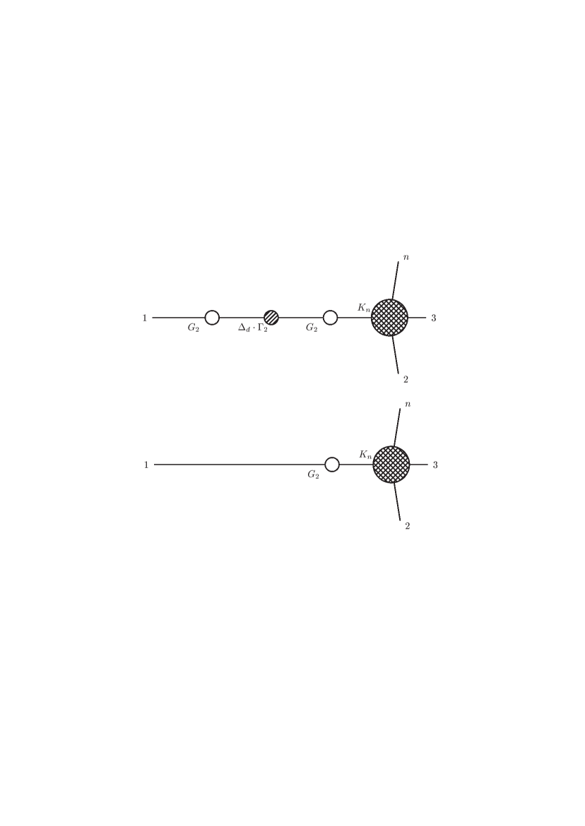
Figure 1: Cancellation of on-shell poles in the dilatation transformation

Before completing the proof, two things have to be prepared. We have realized

$$2(1-p^{2}\partial_{p^{2}})\widetilde{\Gamma}_{2}{(p,-p)}+(\beta_{\lambda}\partial_{\lambda}-\gamma)\widetilde{\Gamma}_{2}{(p,-p)}$$

$$=\alpha_{m}{\Delta}_{d}\cdot\widetilde{\Gamma}_{2}{(p,-p)},$$ (171)

from which the relation between the residue $r$ and the insertion into the 1PI two-point Green function ${\Delta}_{d}\cdot\widetilde{\Gamma}_{2}$ is derived to be

$${\frac{-2m^{2}}{r}}=\alpha_{m}\Delta_{d}\cdot\widetilde{\Gamma}_{2}|_{p^{2}=m^{2}},$$ (172)

which is consistent with the normalization conditions (23). The other crucial point is that the residue $r$ can be determined in the following way,

$$\lim_{p^{2}\to m^{2}}(p^{2}-m^{2})\widetilde{\Delta}(p)=i\hbar\,r,$$ (173)

which is equivalent to ${\frac{1}{r}}$$=$ $\partial_{p^{2}}\,\widetilde{\Gamma}_{2}(p,-p)|_{p^{2}=m^{2}}$.

Now, we can show that the expression (A) is zero by applying the relation between $\Delta_{d}\cdot G_{2}$ and $\Delta_{d}\cdot\Gamma_{2}$,

$$\Delta_{d}\cdot G_{2}(x,z)=\int{\rm d}^{4}z_{1}\int{\rm d}^{4}z_{2}\,G_{2}(x,z_{1})G_{2}(z,z_{2})\Delta_{d}\cdot\Gamma_{2}(z_{1},z_{2}).$$ (174)

The proof means that ${\Delta}^{\prime}_{d}\cdot S_{n}$ only includes the contributions from the local integral insertion $\Delta_{d}$ into the internal propagators of the Green function $G_{n}$, and hence the amputation of the external propagators in ${\Delta}^{\prime}_{d}\cdot S_{n}$ is well-defined.

One remark is stated on our proof. It is based on the Legendre transformation, the skeleton expansion of the Green function, the definition of the residue $r$ and the on-shell renormalization conditions. So, it is independent of choices of both regularization schemes and renormalization procedures.

Appendix B On the on-shell poles in $\alpha\Delta_{k}^{\prime}\cdot S_{A,n}\mid_{P}$

Whether $\alpha\Delta_{k}^{\prime}\cdot S_{A,n}$ contains the on-shell poles or not is a serious problem in calculating the special conformal transformation of the S-matrix. If this was so, the amputation of external propagators cannot be well-defined. In the following, we will try to gain some insights. With $\alpha\Delta_{k}^{\prime}\cdot S_{A,n}$ given by

$$\alpha\Delta_{k}^{\prime}\cdot S_{A,n}:=2m^{2}\,\sum_{l=1}^{n}\,{\mathcal{F}}^{A}_{n}(x,\check{x}_{l};p)(2\alpha x_{l})\,G_{n}+{\frac{i}{\hbar}}\alpha_{m}\,{\mathcal{F}}^{A}_{n}(x;p)\alpha\Delta_{k}\cdot G_{n},$$ (175)

it is necessary to judge whether the sum of the two terms

$${\frac{i}{\hbar}}\int{\rm d}^{4}x_{1}e^{i\,p_{1}x_{1}}\left(2\,m^{2}(2\alpha x_{1})G_{2}(x_{1},y_{1})+{\frac{i}{\hbar}}\alpha_{m}(\Box_{x_{1}}+m^{2})\,\alpha\Delta_{k}\cdot G_{2}(x_{1},y_{1})\right)$$ (176)

vanishes in the on-shell limit. The strategy is the same as in the case of the dilatation transformation. Its diagrammatic interpretation is also shown in the FIG. 1, except that the symbol $\Delta_{d}\cdot\Gamma_{2}$ is changed to $\alpha\Delta_{k}\cdot\Gamma_{2}$.

By means of the Fourier transformation, $\alpha\Delta_{k}\cdot\Gamma_{2}(x_{1},x_{2})$ can be represented by

$$\alpha\Delta_{k}\cdot\Gamma_{2}(x_{1},x_{2})=\int{\frac{{\rm d}^{4}p_{1}}{(2\pi)^{4}}}e^{-ip_{1}(x_{1}-x_{2})}(2\alpha x_{2})[{\textstyle\frac{1}{2}}\phi^{2}(0)]_{2}\cdot\widetilde{\Gamma}_{2}(p_{1},-p_{1})$$

$$+\int{\frac{{\rm d}^{4}p_{1}}{(2\pi)^{4}}}e^{-ip_{1}(x_{1}-x_{2})}(-2i\alpha{\frac{\partial}{\partial p}})[{\textstyle\frac{1}{2}}\phi^{2}(p)]_{2}\cdot\widetilde{\Gamma}_{2}(p_{1},-p-p_{1})\mid_{p=0},$$ (177)

so the $\alpha\Delta_{k}\cdot G_{2}(x_{1},y_{1})$ is denoted by

$$\alpha\Delta_{k}\cdot G_{2}(x_{1},y_{1}) = \int{\frac{{\rm d}^{4}p_{1}}{(2\pi)^{4}}}{\frac{i\hbar\,e^{-ip_{1}x_{1}}}{\widetilde{\Gamma}_{2}(p_{1},-p_{1})}}[{\textstyle\frac{1}{2}}\phi^{2}(0)]_{2}\cdot\widetilde{\Gamma}_{2}(p_{1},-p_{1})$$ (178)

$$\times(-2i\alpha{\frac{\partial}{\partial p_{1}}}){\frac{i\hbar\,e^{ip_{1}y_{1}}}{\widetilde{\Gamma}_{2}(p_{1},-p_{1})}}$$

$$+\int{\frac{{\rm d}^{4}p_{1}}{(2\pi)^{4}}}{\frac{i\hbar\,e^{-ip_{1}x_{1}}}{\widetilde{\Gamma}_{2}(p_{1},-p_{1})}}{\frac{i\hbar\,e^{ip_{1}y_{1}}}{\widetilde{\Gamma}_{2}(p_{1},-p_{1})}}$$

$$\times(-2i\alpha{\frac{\partial}{\partial p}})[{\textstyle\frac{1}{2}}\phi^{2}(p)]_{2}\cdot\widetilde{\Gamma}_{2}(p_{1},-p-p_{1})\mid_{p=0}.$$

Hence, in $\alpha\Delta_{k}^{\prime}\cdot S_{A,n}$, the term $\mathcal{KP}$ containing all possible on-shell poles is given by

$$\mathcal{KP}:=(\,i\,{\hbar}^{n-1}\alpha_{m}\,r^{{\frac{1}{2}}n})(2i\alpha{\frac{\partial}{\partial p}})$$

$$\left(\sum_{l=1}^{n}\,{\frac{[{\textstyle\frac{1}{2}}\phi^{2}(p)]_{2}\cdot\widetilde{\Gamma}_{2}(p_{l},-p-p_{l})}{\widetilde{\Gamma}_{2}(p_{l},-p_{l})}}\right)_{p=0}\,K_{n}(p_{1},\cdots,p_{n})\mid_{p_{l}^{2}=m^{2}}.$$ (179)

Formally taking the massless limit, $\mathcal{KP}$ will vanish because of the vanishing $\alpha_{m}$.

In the following, for example, the insertion $[{\textstyle\frac{1}{2}}\phi^{2}(p)]_{2}\cdot\widetilde{\Gamma}_{2}(p_{1},-p-p_{1})$ is considered. Due to the Lorentz invariance and the subtraction scheme in the BPHZ renormalization procedure, it is obtained from

$$[{\textstyle\frac{1}{2}}\phi^{2}(p)]_{2}\cdot\widetilde{\Gamma}_{2}(p_{1},-p-p_{1})=R(p^{2},p_{1}^{2},m^{2},p\cdot p_{1})-R(0,0,m^{2},0),$$ (180)

where the symbol $R$ stands for the term without subdivergences. So, the problem changes to the one whether the derivative

$${\frac{\partial R(0,m^{2},p\cdot p_{1})}{\partial p\cdot p_{1}}}\mid_{p=0}$$ (181)

vanishes or not, which cannot be exactly solved in a general sense at least in a massive scalar field theory. Here it will be calculated up to two-loop.

Up to order in $\hbar$, there are two non-vanishing Feynman integrals. The two corresponding Feynman diagrams are illustrated in FIG.2.

Figure 2: Contributions to $\mathcal{KP}$ up to order of $\hbar$

The first diagram is the tree approximation giving the constant value and will vanish when taking the derivative. The second Feynman integral has the form

$${\frac{i\hbar\lambda}{2}}{\frac{\rm d^{4}k}{(2\,\pi)^{4}}}(D_{k}\,D_{p+k}-D_{k}^{2}),$$ (182)

where the symbol $D_{k}$ and $D_{p+k}$ are denoted by

$$D_{k}={\frac{1}{k^{2}-m^{2}}},\qquad D_{p+k}={\frac{1}{(p+k)^{2}-m^{2}}}.$$ (183)

Applying the derivation action ${\frac{\partial}{\partial p}}$ then setting $p$ zero, the second Feynman diagram still contributes zero.

In order of $\hbar^{2}$, there are two types of diagrams, given in FIG.3 and FIG.4. First, consider FIG.3. The first diagram is similar to the second one in FIG. 2, but involves the counterterm as the interaction vertex, then also giving a vanishing result. The second Feynman diagram is the scoop one including one tadpole, and thus giving no contribution. The third one has the Feynman integral with

$${\frac{(i\hbar\lambda)^{2}}{4}}{\frac{\rm d^{4}k_{1}}{(2\,\pi)^{4}}}{\frac{\rm d^{4}k_{2}}{(2\,\pi)^{4}}}(D_{k_{1}}\,D_{p+{k_{1}}}-D^{2}_{k_{1}})(D_{k_{2}}\,D_{p+{k_{2}}}-D^{2}_{k_{2}}),$$ (184)

which also vanishes in the calculation of ${\mathcal{K}P}$.

Figure 3: Vanishing contributions to $\mathcal{KP}$ in order of $\hbar^{2}$

Consider the sunset Feynman diagram in FIG.4.

Figure 4: Non-vanishing contribution to $\mathcal{KP}$ in order of $\hbar^{2}$

The relevant two-loop calculation is carried out to obtain

$$(2i\alpha{\frac{\partial}{\partial p}})\left(\sum_{l=1}^{n}\,{\frac{[{\textstyle\frac{1}{2}}\phi^{2}(p)]_{2}\cdot\widetilde{\Gamma}_{2}(p_{l},-p-p_{l})}{\widetilde{\Gamma}_{2}(p_{l},-p_{l})}}\right)^{(\leq 2)}\mid_{p=0,~{}p_{l}^{2}=m^{2}}$$

$$={\frac{1}{2!(4\pi)^{4}}}(1-{\frac{\pi^{2}}{12}}){\frac{\hbar^{2}\lambda^{2}}{m^{2}}}\sum_{l=1}^{n}\,{\frac{2i\alpha\,p_{l}}{p_{l}^{2}-m^{2}}}\mid_{p_{l}^{2}=m^{2}}.$$ (185)

Therefore, in our case, the term ${\mathcal{K}P}$ is approximated by

$${\mathcal{K}P}={\mathcal{O}}(\hbar^{2}).$$ (186)

It suggests that in the massive scalar field theory $\alpha\Delta_{k}^{\prime}\cdot S_{A,n}\mid_{P}$ has on-shell poles. In order to make ${\mathcal{K}P}$ vanish, there are at least two ways out. The first one is that complicated field theories have to be involved, such as supersymmetrical field theories, see white0 ; white1 . The second one suggests to redefine the special conformal transformation of the off-shell S-matrix element $S_{A,n}$ in the on-shell limit

$$\alpha\mathcal{W}^{K}S_{A,n}\mid_{P}$$ (187)

according to the equation (85)

$$\alpha\mathcal{W}^{K}S_{n}=\alpha\mathcal{W}^{K}S_{A,n}\mid_{P}-4\,i\,m^{2}\sum_{l=1}^{n}\alpha\mathcal{P}^{k}_{l}S^{\prime}_{A,n}\mid_{P},$$ (188)

since $\alpha\mathcal{W}^{K}S_{n}$ has to be finite in a physical sense.

Appendix C Current constructions and charge constructions

As a matter of fact, the S-matrix used in our work is defined in the LSZ reduction procedure. With this approach, the information on the operator formalism can be recovered, such as current constructions, charge constructions and quantum transformations of quantum fields.

For simplification, the moment constructions of the local Ward identity operators can be chosen as follows:

$$\widetilde{\mathbf{w}}_{\mu}^{T}(x) = \partial_{\mu}\phi(x){\frac{\delta}{\delta\phi(x)}}-{\frac{1}{4}}\partial_{\mu}\left(\phi(x){\frac{\delta}{\delta\phi(x)}}\right),$$ (189)

$$\widetilde{\mathbf{w}}_{\mu\nu}^{L}(x) = x_{\mu}\widetilde{\mathbf{w}}_{\nu}^{T}(x)-x_{\nu}\widetilde{\mathbf{w}}_{\mu}^{T}(x),$$ (190)

$$\widetilde{\mathbf{w}}^{D}(x) = x^{\mu}\widetilde{\mathbf{w}}_{\mu}^{T}(x),$$ (191)

$$\widetilde{\mathbf{w}}^{K}_{\nu}(x) = (2x^{\mu}x_{\nu}-\eta^{\mu}_{\nu}x^{2})\widetilde{\mathbf{w}}_{\mu}^{T}(x).$$ (192)

Applying the quantum action principle in the BPHZ renormalization procedure, the energy-momentum tensor $T_{\mu\nu}$ can be calculated from

$$\widetilde{\mathbf{w}}_{\mu}^{T}(x)\cdot\Gamma=-[\partial^{\nu}\,T_{\mu\nu}(x)]\cdot\Gamma.$$ (193)

Then the breaking of the conformal invariance are controlled by the insertion of the trace of the energy-momentum tensor, namely,

$$\widetilde{\mathbf{w}}^{D}\Gamma = -\partial^{\nu}\left[{D_{\nu}}\right]\cdot\Gamma+\left[T^{\nu}_{\nu}\right]\cdot\Gamma,$$ (194)

$$\widetilde{\mathbf{w}}^{K}_{\nu}\Gamma = -\partial^{\mu}\left[{K_{\mu\nu}}\right]\cdot\Gamma+2x_{\nu}\left[T^{\mu}_{\mu}\right]\cdot\Gamma,$$ (195)

where the current $D_{\nu}$ is $x^{\mu}T_{\mu\nu}$ for the dilatation transformation and the current $K_{\mu\nu}$ is $(2x_{\nu}x^{\zeta}-\eta_{\nu}^{\zeta}x^{2})T_{\mu\zeta}$ for the special conformal transformation.

Define the local Ward identity for the space-time translation in the generating functional $Z[J]$ by

$$\widetilde{\mathbf{w}}_{\mu}^{T}(x)Z[J] := \left(J(x)\partial_{\mu}{\frac{\delta}{\delta J(x)}}-{\frac{1}{4}}\partial_{\mu}(J(x){\frac{\delta}{\delta J(x)}})\right)Z[J]$$ (196)

$$= {\frac{i}{\hbar}}\partial^{\nu}[T_{\mu\nu}]\cdot Z[J].$$

It can be realized in the Green function via

$$\widetilde{\mathbf{w}}_{\mu}^{T}(x)G_{n} = \sum_{l=1}^{n}\delta(x-x_{l})\partial^{x}_{\mu}G_{n}(x,x_{1},\cdots,\check{x}_{l},\cdots,x_{n})$$ (197)

$$-{\frac{1}{4}}\sum_{l=1}^{n}\partial^{x}_{\mu}\left(\delta(x-x_{l})G_{n}(x,x_{1},\cdots,\check{x}_{l},\cdots,x_{n})\right)$$

$$= {\frac{i}{\hbar}}\partial^{\nu}[T_{\mu\nu}]\cdot G_{n}(x_{1},\cdots,x_{n}),$$

where $\check{x}_{l}$ indicates that $\check{x}_{l}$ is missing in the string of variables. Furthermore, the local Ward identity for space-time translations in the momentum space is given by

$$\widetilde{\mathbf{w}}_{\mu}^{T}(p)G_{n} = -i\sum_{l=1}^{n}\left((p_{\mu}+p_{l,\mu})-{\frac{1}{4}}p_{\mu}\right)G_{n}(p+p_{l},p_{1},\cdots,\check{p}_{l},\cdots,p_{n})$$ (198)

$$= {\frac{i}{\hbar}}(-ip^{\nu})[T_{\mu\nu}(p)]\cdot G_{n}(p_{1},\cdots,\cdots,p_{n}),$$

which can be transfered into the form

$${\frac{i}{\hbar}}(-ip^{\nu})[T_{\mu\nu}(p)]\cdot S_{n}(p_{1},\cdots,\cdots,p_{n})$$

$$=-i\sum_{l=1}^{n}\left((p_{\mu}+p_{l,\mu})-{\frac{1}{4}}p_{\mu}\right)(-ir^{-{\textstyle\frac{1}{2}}})^{n}\prod_{j=1}^{n}(p_{j}^{2}-m^{2})$$

$$\times G_{n}(p+p_{l},p_{1},\cdots,\check{p}_{l},\cdots,p_{n})|_{P}.$$ (199)

In the on-shell limit and in case of $p$ being nonzero and the right hand side being zero, the conservation of the energy-momentum tensor is obtained by

$$p^{\nu}\hat{T}_{\mu\nu}(p)=0,$$ (200)

which is given in coordinate space by

$$\partial^{\nu}\hat{T}_{\mu\nu}=0.$$ (201)

Hence the four-momentum charge $\hat{P}_{\mu}$ is defined as

$$\hat{P}_{\mu}:=\int\,{\rm d}^{3}x\,\hat{T}_{\mu 0}.$$ (202)

Here all involved operators are defined in the asymptotic Hilbert space $\mathcal{H}$ satisfying

$$\mathcal{H}=\mathcal{H}_{\rm in}=\mathcal{H}_{\rm out}.$$ (203)

Similarly, for the other conformal transformations, the corresponding expressions can be also set up

$$\partial^{a}\hat{M}_{\mu\nu a} = 0,$$

$$\partial^{\mu}\hat{D}_{\mu} = \hat{T}^{\nu}_{\nu},$$

$$\partial^{\mu}\hat{K}_{\mu\nu} = 2x_{\nu}\hat{T}^{\mu}_{\mu},$$ (204)

where $\hat{M}_{\mu\nu a}$, $\hat{D}_{\mu}$, and $\hat{K}_{\nu\mu}$ are respectively given by

$$\hat{M}_{\mu\nu a}=x_{\mu}\hat{T}_{\nu a}-x_{\nu}\hat{T}_{\mu a},\qquad\hat{D}_{\mu}=x^{\nu}\hat{T}_{\mu\nu},\qquad\hat{K}_{\nu\mu}=(2x_{\nu}x^{\zeta}-\eta_{\nu}^{\zeta}x^{2})\hat{T}_{\mu\zeta}.$$ (205)

Then the charge $M_{\mu\nu}$ for the Lorentz rotations is denoted by $\int\,{\rm d}^{3}x\hat{M}_{\mu\nu 0}\,$. But the charges for both the dilatation transformation and for the special conformal transformation cannot easily be found out.

To derive the quantum transformations of the quantum field operator $\hat{\Phi}$, the LSZ reduction procedure can be applied on the both sides of the local Ward identity (198), namely

$${\frac{i}{\hbar}}(-ir^{-{\textstyle\frac{1}{2}}})^{n}\prod_{j=2}^{n}(p_{j}^{2}-m^{2})(-ip^{\nu})[T_{\mu\nu}(p)]\cdot G_{n}(p_{1},\cdots,\cdots,p_{n})|_{P}$$

$$=-i\sum_{l=1}^{n}\left((p_{\mu}+p_{l,\mu})-{\frac{1}{4}}p_{\mu}\right)(-ir^{-{\textstyle\frac{1}{2}}})^{n}\prod_{j=2}^{n}(p_{j}^{2}-m^{2})$$

$$\times\,G_{n}(p+p_{l},p_{1},\cdots,\check{p}_{l},\cdots,p_{n})|_{P}.$$ (206)

In the on-shell limit, the above formalism is related to

$$-i\left((p_{\mu}+p_{l,\mu})-{\frac{1}{4}}p_{\mu}\right)\hat{\Phi}(p+p_{1})={\frac{i}{\hbar}}(-ip^{\nu})\mathcal{T}\left(\hat{T}_{\mu\nu}(p)\hat{\Phi}(p_{1})\right),$$ (207)

where the symbol $\mathcal{T}$ denotes the time-ordering defined in the coordinate space. Then the action of the local Ward identity operator for space-time translations on the quantum field operator $\hat{\Phi}(x)$ in coordinate space is given by

$$\widetilde{\mathbf{w}}_{\mu}^{T}(x)\hat{\Phi}(x_{1}) := \partial_{\mu}^{x}\hat{\Phi}(x)\delta^{4}(x-x_{1})-{\frac{1}{4}}\partial_{\mu}^{x}(\hat{\Phi}(x)\delta^{4}(x-x_{1}))$$ (208)

$$= {\frac{i}{\hbar}}\partial^{\nu}\mathcal{T}\left(\hat{T}_{\mu\nu}(x)\hat{\Phi}(x_{1})\right).$$

The similar equations for the other conformal transformations can be also obtained by

$$(x_{\mu}\widetilde{\mathbf{w}}_{\nu}^{T}(x)-x_{\nu}\widetilde{\mathbf{w}}_{\mu}^{T}(x))\hat{\Phi}(x_{1}) = {\frac{i}{\hbar}}\partial^{a}\mathcal{T}\left(\hat{M}_{\mu\nu a}(x)\hat{\Phi}(x_{1})\right),$$ (209)

$$x^{\mu}\widetilde{\mathbf{w}}_{\mu}^{T}(x)\hat{\Phi}(x_{1}) = {\frac{i}{\hbar}}\partial^{\mu}\mathcal{T}\left(\hat{D}_{\mu}(x)\hat{\Phi}(x_{1})\right)$$ (210)

$$-{\frac{i}{\hbar}}\mathcal{T}\left(\hat{T}^{\nu}_{\nu}(x)\hat{\Phi}(x_{1})\right),$$

$$(2x_{\nu}x^{\mu}-\eta_{\nu}^{\mu}x^{2})\widetilde{\mathbf{w}}_{\mu}^{T}(x)\hat{\Phi}(x_{1}) = {\frac{i}{\hbar}}\partial^{\mu}\mathcal{T}\left(\hat{K}_{\mu\nu}(x)\hat{\Phi}(x_{1})\right)$$ (211)

$$-{\frac{i}{\hbar}}2x_{\nu}\mathcal{T}\left(\hat{T}^{\mu}_{\mu}(x)\hat{\Phi}(x_{1})\right).$$

The quantum transformations of the quantum field $\hat{\Phi}$ for space-time translations and Lorentz rotations are obtained by integrating

$$\int^{x^{0}+\varepsilon}_{x^{0}-\varepsilon}{\rm d}x_{1}^{0}\int{\rm d}^{3}x_{1}$$ (212)

on both sides of the above equations (208) and (209), namely

$$\delta^{T}_{\mu}\,\hat{\Phi} := \partial_{\mu}\hat{\Phi}={\frac{i}{\hbar}}[\hat{P}_{\mu},\hat{\Phi}],$$

$$\delta^{L}_{\mu\nu}\,\hat{\Phi} := (x_{\mu}\partial_{\nu}-x_{\nu}\partial_{\mu})\hat{\Phi}={\frac{i}{\hbar}}[\hat{M}_{\mu\nu},\hat{\Phi}].$$ (213)

In the cases of the dilatation transformation and the special conformal transformation, the quantum transformations in the free(or asymptotic free) field theory are constructed by

$$\delta^{D}\hat{\phi}_{\rm in}(x) := (1+x\partial_{x})\hat{\phi}_{\rm in}(x)={\frac{i}{\hbar}}[\hat{D},\hat{\phi}_{\rm in}(x)],$$

$$\delta^{K}_{\nu}\hat{\phi}_{\rm in}(x) := \left((2x_{\nu}x^{\mu}-\eta_{\nu}^{\mu}x^{2})\partial_{\mu}+2x_{\nu}\right)\hat{\phi}_{\rm in}(x)={\frac{i}{\hbar}}[\hat{K}_{\nu},\hat{\phi}_{\rm in}(x)],$$ (214)

where $\hat{D}$ is the charge for the dilatation transformation and $\hat{K}_{\nu}$ is the charge for the special conformal transformation.

References

- (1) H. Epstein, V. Glaser, Ann. Inst. Henri Poincaré 19, 211 (1973)
- (2) R. Coleman, J. Mandula, Phys. Rev. 159, 1251 (1967)
- (3) R. Haag, T. Lopuszanski, M. Sohnius, Nucl. Phys. B 88, 257 (1975)
- (4) W. Zimmermann, Commun. Math.Phys. 76, 39 (1980)
- (5) C. Becchi, A. Rouet, R. Stora, Commun. Math.Phys. 42, 127 (1975)
- (6) C. Becchi, A. Rouet, R. Stora, Ann. Phys. 98, 287 (1976)
- (7) K. Sibold, Störungtheoretische Renormierung Quantisierung von Eichtheorieen (unpublished, 1993)
- (8) O. Piguet, S.P. Sorella, Algebraic Renormalization: Perturbative Renormalization, Symmetries and Anomalies (Springer 1995)
- (9) A. Boresch, O. Moritsch, M. Schweda, T. Sommer, H. Zerrouki, S. Emery, Applications of Noncovariant Gauges in the Algebraic Renormalization Procedure (World Scientific 1998)
- (10) J.H. Lowenstein, Phys. Rev. D 4, 2281 (1971)
- (11) J.H. Lowenstein, Commun. Math.Phys. 24, 1 (1971)
- (12) Y.M.P. Lam, Phys. Rev. D 6, 2145 (1972)
- (13) Y.M.P. Lam, Phys. Rev. D 7, 2943 (1973)
- (14) W. Zimmermann, Commun. Math.Phys. 11, 208 (1969)
- (15) W. Zimmermann, Ann. Phys. (N. Y.) 77, 536 (1973)
- (16) W. Zimmermann, Ann. Phys. (N. Y.) 77, 570 (1973)
- (17) C. G. Callan, Phys. Rev. D 2, 1541 (1970)
- (18) K. Symanzik, Commun. Math.Phys. 18, 227 (1970)
- (19) T. Kugo, I. Ojima, Prog. Theor. Phys. 60, 1869 (1978)
- (20) T. Kugo, I. Ojima, Prog. Theor. Phys. 61, 294 (1979)
- (21) E. Kraus, K. Sibold, Nucl. Phys. B 372, 113 (1992)
- (22) E. Kraus, K. Sibold, Nucl. Phys. B 398, 125 (1993)
- (23) S. Weinberg, Phys. Rev. 18, 838 (1960)
- (24) R. Coleman, R. Jackiw, Ann. Phys. 67, 552 (1971)
- (25) D. Grigore, Scale Invariance in the Causal Approach to Renormalization Theory, hep-th/0004163
- (26) A. Aste, G. Scharf, Int. J. Mod. Phys. A 14, 3421 (1999)
- (27) E. Kraus, C. Rupp, K. Sibold, Eur. Phys. J. C 24, 631 (2002)
- (28) E. Kraus, Nucl. Phys. B 620, 55 (2002), hep-th/0107239
- (29) P.L. White, Class. Quant. Grav. 9, 413 (1992)
- (30) P.L. White, Class. Quant. Grav. 9, 1663 (1992)