ROM2F-03/07 hep-th/0305224 Magnetized Four-Dimensional $Z_{2}\times Z_{2}$ Orientifolds

We study deformations of $Z_{2}\times Z_{2}$ (shift-)orientifolds in four dimensions in the presence of both uniform Abelian internal magnetic fields and quantized NS-NS $B_{ab}$ backgrounds, that are shown to be equivalent to asymmetric shift-orbifold projections. These models are related by $T$-duality to orientifolds with $D$-branes intersecting at angles. As in corresponding six-dimensional examples, $D9$-branes magnetized along two internal directions acquire a charge with respect to the R-R six form, contributing to the tadpole of the orthogonal $D5$-branes (“brane transmutation”). The resulting models exhibit rank reduction of the gauge group and multiple matter families, due both to the quantized $B_{ab}$ and to the background magnetic fields. Moreover, the low-energy spectra are chiral and anomaly free if additional $D5$-branes longitudinal to the magnetized directions are present, and if there are no Ramond-Ramond tadpoles in the corresponding twisted sectors of the undeformed models.

1. Introduction

Perturbative type I vacua [1, 2, 3] (for reviews see [4, 5]) are a small corner in the moduli space of the unified underlying and yet poorly understood eleven dimensional M-theory [6]. Nowadays, however, they are the most promising perturbative models to test possible “stringy” effects at the next generation of accelerators [7]. Indeed, while in the usual heterotic SUSY-GUT scenarios [9] the string scale is directly tied to the Planck scale, making it hard to conceive probes of low-energy effects, the type I string scale is basically an independent parameter, that can be lowered down to a few TeV’s [10]. In this setting, and more generally in the context of “brane-world scenarios” [11, 7], the gauge degrees of freedom are confined to some (stacks of) branes while the gravitational interactions invade the whole higher dimensional spacetime. In order to respect the experimental limits on gravitational interactions, the extra dimensions orthogonal to the branes could be up to sub-millimeter size [12], while the extra dimensions longitudinal to the branes should be quite tiny (at least of TeV scale) but still testable in future experiments. In this context, however, several aspects of the conventional Standard Model picture like, for instance, the problem of scale hierarchies and the unification of the running coupling constants at a scale of order $10^{16}GeV$ in the MSSM desert hypothesis, have to be reconsidered [7, 5, 8]. Some other issues, like supersymmetry breaking, find instead new possibilities in type I perturbative vacua.

There are basically four known ways to break supersymmetry within String Theory. The first is to combine left and right moving modes in a non-supersymmetric fashion, like for instance in the type $0$ models [13] and in the corresponding lower dimensional compactifications and orientifolds [2, 14, 15, 16]. Some type I-like instances, the type $0^{\prime}$B and its compactifications [14], are also free of the tachyons that typically plague this kind of models. The second is the generalization to String Theory of the Scherk-Schwarz mechanism [17], available also in the heterotic case, in which the breaking is due to a generalized Kaluza-Klein compactification that involves different periodicities for bosons and fermions, thereby not respecting supersymmetry [18]. In this framework, the scale of supersymmetry breaking is inversely proportional to the volume of the internal manifold and some residual global supersymmetries may be left at tree level on some branes (“brane supersymmetry”) [19, 20]. The third possibility is related to models with supersymmetry non linearly realized on some branes, as a result of the simultaneous presence of branes and antibranes of the same [21, 22, 23] or of different types [24, 22, 25], or of the introduction of “exotic” orientifold planes [26]. These are referred to as “brane supersymmetry breaking” models, and the corresponding scale of supersymmetry breaking can be tied generically to the string scale. Finally, supersymmetry can be broken [27, 28, 29] by the introduction of internal magnetic fields [30] in the open sectors [28, 31, 32, 33]. In refs. [31, 32], six-dimensional $(T^{2}\times T^{2})/Z_{2}$ orientifold models with a pair of internal magnetic fields turned on inside the internal tori have been discussed in detail.

In this paper we extend the construction of [31, 32] to four dimensional models obtained as magnetic deformations of $Z_{2}\times Z_{2}$ orientifolds, possibly combined with momentum or winding shifts along some of the internal directions [20, 22]. Some preliminary results have already appeared in refs. [34]. As in the six-dimensional models of [31, 32], for generic values of the magnetic fields Nielsen-Olesen instabilities [35] manifest themselves in the presence of tachyonic excitations, and supersymmetry is broken due to the unpairing of states of different spins. However, the compactness of the internal space allows self-dual or antiself-dual Abelian field configurations with non-vanishing instanton number, that can compensate the R-R charge excess, eliminating the tachyons and retrieving supersymmetry if the BPS bound is saturated, or giving rise to “brane supersymmetry breaking” models if the magnetized $D9$-branes transmute into anti $D5$-branes [31, 32]. The resulting models exhibit several interesting features, to wit Chan-Paton gauge groups of reduced rank and several families of matter multiplets, linked in a natural way to the degeneracy of the Landau levels. Moreover, in the presence of $D$-branes longitudinal to the directions along which the magnetic fields are turned on, the four dimensional models can also be chiral. It should be stressed that these models with internal background (open) magnetic fields are connected by T-duality to orientifolds with $D$-branes intersecting at angles [36, 37, 38, 39, 40, 41, 42, 43, 44], that have received much attention in the last few years in attempts to recover (extensions of) the Standard Model as low-energy limits of String Theory or M-theory. A byproduct of this analysis is a precise link between a quantized NS-NS $B_{ab}$ and shift-orbifolds.

This paper is organized as follows: in Section 2, after a brief discussion of the relation between shifts and the quantized NS-NS two form $B_{ab}$, we shortly review the basic facts characterizing $Z_{2}\times Z_{2}$ (shift-)orientifolds in its presence. In Section 3 we discuss general aspects of the inclusion of uniform internal Abelian magnetic fields in the open-string sector and shortly review the models in [31]. In Section 4 we describe four dimensional examples based on magnetic deformations of the $Z_{2}\times Z_{2}$ (shift-)orientifolds previously introduced. Section 5 is devoted to one “brane supersymmetry breaking” example and finally Section 6 contains our Conclusions. Notations, conventions and Tables are displayed in the Appendices. In particular, Appendix A collects the relevant lattice sums that enter the one-loop partition functions. The $Z_{2}\times Z_{2}$ characters are defined in Appendix B, while Appendix C is a collection of Tables that summarize massless spectra, gauge groups and tadpole cancellation conditions for all the models considered in this paper.

2. $Z_{2}\times Z_{2}$ Orientifolds

In this Section we review some four dimensional type I vacua obtained as orientifolds of $Z_{2}\times Z_{2}$ orbifolds, or of freely acting $Z_{2}\times Z_{2}$ shift-orbifolds. The starting point is an orbifold of the type IIB superstring compactified on an internal six-torus that, without any loss of generality for our purposes, can be chosen to be a product of three two-tori $T^{45}$, $T^{67}$ and $T^{89}$ along the three complex directions $Z^{1}=X^{4}+iX^{5}$, $Z^{2}=X^{6}+iX^{7}$ and $Z^{3}=X^{8}+iX^{9}$. Each two-torus can be equipped with a NS-NS background two-form $B_{i}$ of rank $r_{i}$ (with $r_{i}=0$ or $2$) that, if the orientifold projection is induced by the world-sheet parity operator $\Omega$, is a discrete modulus and may thus take only quantized values [45, 46]. The orbifold group will be taken to be the combination of the $Z_{2}\times Z_{2}$ generated by the elements

$$g:(+,-,-)\qquad{\rm and}\qquad h:(-,-,+)\quad,$$ (2.1)

where the minus signs indicate the two-dimensional $Z_{2}$ inversion of the corresponding coordinates $(Z^{i}\rightarrow-Z^{i})$, with momenta and/or winding shifts along the real part of (some of) the three complex directions.

The conventional $Z_{2}\times Z_{2}$ orbifolds, allowing for the introduction of a “discrete torsion”[47], give rise to supersymmetric orientifolds [48, 49, 39] as well as to orientifolds with “brane supersymmetry breaking” [22]. Moreover, the freely acting $Z_{2}\times Z_{2}$ (shift-)orbifolds produce ten classes of orientifolds with different amounts of supersymmetry (models with “brane supersymmetry” [19, 20]), together with a huge number of variants with brane-antibrane pairs and “brane supersymmetry breaking”[22].

2.1 NS-NS $B_{ab}$ and Shifts

Before moving to the detailed analysis of the models, it is worth clarifying the relation between a non-vanishing discretized NS-NS two form $B_{ab}$ on orientifolds [45, 46] and momentum and winding shifts. In particular, we want to show that the presence of a quantized NS-NS two-form field $B_{ab}$ on a two-torus is exactly equivalent to an asymmetric shift-orbifold in which a momentum shift along the first direction of the torus is accompanied by a winding shift along the other direction. For simplicity, let us take for the two-torus a product of circles both of radius $R$. Parametrizing the discretized two form as [45]

$$B\ =\ \frac{\alpha^{\prime}}{2}\left(\begin{array}[]{rrrr}0&1\\ -1&0\end{array}\right)\quad,$$ (2.4)

the generalized momenta of eqs. (A1, A2) reduce to the expressions

$$p_{{\rm(L,R)}\,a}\ =\ m_{a}^{\prime}\ \pm\ \frac{1}{\alpha^{\prime}}\ g_{ab}\ n^{b}\qquad,$$ (2.5)

where $m_{a}^{\prime}\,=\,m_{a}\,-\,\frac{1}{2}\,\epsilon_{ab}\,n^{b}$. The presence of $B_{ab}$ makes the $m_{a}^{\prime}$’s integers or half-integers depending on the oddness or evenness of the integer $n^{a}$’s. As a result, omitting the prime on the dummy $m$-variables for the rest of this Section, the torus partition function of eq. (A3) can be decomposed in the form

$$\!\!\!\Lambda(B)\!\!\! = \!\!\!\Lambda(m_{1},m_{2},2n_{1},2n_{2})+\Lambda(m_{1}+1/2,m_{2},2n_{1},2n_{2}+1)$$

$$+ \!\!\!\Lambda(m_{1},m_{2}+1/2,2n_{1}+1,2n_{2})+\Lambda(m_{1}+1/2,m_{2}+1/2,2n_{1}+1,2n_{2}+1)\,,$$

where $\Lambda(m_{1},m_{2},n_{1},n_{2})$ denotes the two-dimensional lattice sum over momenta $m_{a}/R$ and windings $n^{a}R$.

The same partition function can be obtained as an asymmetric shift-orbifold. Indeed, projecting the conventional ($B=0$) $\Lambda(m_{1},m_{2},n_{1},n_{2})$ under the action of a $p_{1}w_{2}$ shift and completing the modular invariant with the addition of twisted sectors, the resulting partition function is

$$\Lambda(p_{1}w_{2})\!\!\! = \!\!\!\frac{1}{2}\ \bigl{[}\,\Lambda(m_{1},m_{2},n_{1},n_{2})+(-1)^{m_{1}+n_{2}}\,\Lambda(m_{1},m_{2},n_{1},n_{2})$$

$$+ \!\!\!\Lambda(m_{1},m_{2}+1/2,n_{1}+1/2,n_{2})+(-1)^{m_{1}+n_{2}}\,\Lambda(m_{1},m_{2}+1/2,n_{1}+1/2,n_{2})\,\bigr{]}\ .$$

This expression is exactly the one in eq. (2.1) after doubling the radius $(R\rightarrow 2R)$ along the first direction. Thus, it should not come as a surprise that in some cases the effect of the shifts can be compensated by the presence of a quantized $B_{ab}$. However, all the models in this paper display a reduction of the rank of the Chan-Paton group when a non-vanishing quantized $B_{ab}$ is turned on. The reason is that the shifts we consider affect only one real coordinate of the tori, rather than two as in the previous asymmetric shift-orbifold construction. Nonetheless, in some cases, the shifts make the multiplicities of the matter multiplets independent of the rank of $B_{ab}$. By $T$-duality, other allowed discrete moduli [52, 53, 54] like, for instance, the off-diagonal components of the metric in orientifolds of the type IIA superstring, can also be related to suitable shift-orbifolds.

A nice geometric interpretation of the rank reduction of the Chan-Paton groups can also be given resorting to the asymmetric shift-orbifold description of $B_{ab}$. As we shall extensively see in the next Sections, a momentum shift orthogonal to $D$-branes splits them into multiple images. After a $T$-duality along the second direction of the two-torus, the $p_{1}w_{2}$ becomes a $p_{1}p_{2}$ shift-orbifold, that admits orientifold projections containing $D1$-branes parallel to $p_{1}$ and orthogonal to $p_{2}$. The corresponding annulus amplitude can be written

$${\cal A}\ =\ \frac{1}{2}\ N^{2}\ \big{(}\,P_{1}+P_{1}^{1/2}\,\big{)}\ \big{(}\,W_{2}+W_{2}^{1/2}\,\big{)}\ ,$$ (2.8)

where $P_{i}$ and $W_{i}$ are the usual one-dimensional momentum and winding lattice sums [45], respectively, while $P_{i}^{1/2}$ and $W_{i}^{1/2}$ are the corresponding shifted ones, and the consistent Möbius amplitude, describing the unoriented projection, is

$${\cal M}\ =\ -\frac{1}{2}\ N\ \big{(}\,\hat{P}_{1}\,\hat{W}_{2}\,+\,\hat{P}_{1}^{1/2}\,\hat{W}_{2}^{1/2}\,\big{)}\ .$$ (2.9)

Eqs. (2.8, 2.9) neatly display the expected doublet structure of the $D1$-brane configuration, and the analysis of the tadpole cancellation conditions reveals the related rank reduction of the Chan-Paton group. For instance, an equivalent eight-dimensional $p_{1}p_{2}$ shift-orientifold compactification of the type IIB superstring, would yield type I models with an $SO(16)$ gauge group, thus providing a rank reduction by a factor of two.

2.2 $Z_{2}\times Z_{2}$ Models and Discrete Torsion

Let us now turn to the analysis of the $Z_{2}\times Z_{2}$ models. Aside from the identity, the $Z_{2}\times Z_{2}$ elements can be grouped together in the matrix

$$\sigma_{0}\ =\ \left(\begin{array}[]{rrrr}+&-&-\\ -&+&-\\ -&-&+\end{array}\right)\quad,$$ (2.13)

whose rows represent the action of $g$, $f=g\circ h$ and $h$ on the three internal torus coordinates $Z^{i}$. The one-loop closed partition function can be obtained supplementing the $Z_{2}\times Z_{2}$ projections of the toroidal amplitude with the inclusion of three twisted sectors, located at the three fixed tori, to complete the modular invariant. There are actually two options, related to the freedom of introducing a discrete torsion [47], i.e. a relative sign between two disconnected orbits of the modular group. The result is

$${\cal T}\!\!\! = \!\!{1\over 4}\Biggl{\{}|T_{oo}|^{2}\Lambda_{1}(B_{1})\Lambda_{2}(B_{2})\Lambda_{3}(B_{3})+\big{[}\,|T_{og}|^{2}\Lambda_{1}(B_{1})+|T_{of}|^{2}\Lambda_{2}(B_{2})+|T_{oh}|^{2}\Lambda_{3}(B_{3})\,\big{]}\ \left|{4\eta^{2}\over\vartheta_{2}^{2}}\right|^{2}$$ (2.14)

$$+ \big{[}\ |T_{go}|^{2}\Lambda_{1}(B_{1})+|T_{fo}|^{2}\Lambda_{2}(B_{2})+|T_{ho}|^{2}\Lambda_{3}(B_{3})\ \big{]}\ \left|{4\eta^{2}\over\vartheta_{4}^{2}}\right|^{2}$$

$$+ \big{[}\ |T_{gg}|^{2}\Lambda_{1}(B_{1})+|T_{ff}|^{2}\Lambda_{2}(B_{2})+|T_{hh}|^{2}\Lambda_{3}(B_{3})\ \big{]}\ \left|{4\eta^{2}\over\vartheta_{3}^{2}}\right|^{2}$$

$$+ \omega\left(|T_{gh}|^{2}+|T_{gf}|^{2}+|T_{fg}|^{2}+|T_{fh}|^{2}+|T_{hg}|^{2}+|T_{hf}|^{2}\right)\left|{8\eta^{3}\over\vartheta_{2}\vartheta_{3}\vartheta_{4}}\right|^{2}\Biggr{\}}\quad,$$

where the $\Lambda_{i}$’s are the two-dimensional Narain lattice sums for the three internal tori (see Appendix A), that depend on the two-dimensional blocks $(B_{i})$ of the NS-NS two-form $B_{ab}$, and $\omega=\pm 1$ is the sign associated to the discrete torsion. We have expressed the torus amplitude in terms of the 16 quantities $(i=o,g,h,f)$

$$T_{io} = \tau_{io}+\tau_{ig}+\tau_{ih}+\tau_{if}\quad,\qquad T_{ig}=\tau_{io}+\tau_{ig}-\tau_{ih}-\tau_{if}\quad,$$

$$T_{ih} = \tau_{io}-\tau_{ig}+\tau_{ih}-\tau_{if}\quad,\qquad T_{if}=\tau_{io}-\tau_{ig}-\tau_{ih}+\tau_{if}\quad,$$ (2.15)

where the $16$ $Z_{2}\times Z_{2}$ characters $\tau_{il}$ [48], combinations of products of level-one SO(2) characters, are displayed in Appendix B. The geometric model, related to the “charge conjugation” modular invariant, corresponds to the choice $\omega=-1$, as can be deduced from the massless spectra reported in Table 2. It is a compactification on (a singular limit of) a Calabi-Yau threefold with Hodge numbers $(h_{11}=51,h_{21}=3)$, while the $\omega=1$ choice, linked in this context to the T-dual compactification, leads to (a singular limit of) the mirror symmetric Calabi-Yau threefold, with $h_{11}=3,h_{21}=51$.

The starting point for the orientifold construction are the Klein-bottle amplitudes

$${\cal K}\!\! = \!\!\frac{1}{8}\biggl{\{}(P_{1}P_{2}P_{3}+2^{-4}P_{1}W_{2}(B_{2})W_{3}(B_{3})+2^{-4}W_{1}(B_{1})P_{2}W_{3}(B_{3})+2^{-4}W_{1}(B_{1})W_{2}(B_{2})P_{3})T_{oo}$$ (2.16)

$$+ \!\!2\times 16\bigl{[}2^{-\frac{r_{2}}{2}-\frac{r_{3}}{2}}\omega_{1}(P_{1}+\omega\,2^{-2}W_{1}(B_{1}))T_{go}+2^{-\frac{r_{1}}{2}-\frac{r_{3}}{2}}\omega_{2}(P_{2}+\omega\,2^{-2}W_{2}(B_{2}))T_{fo}$$

$$+ \!\!2^{-\frac{r_{1}}{2}-\frac{r_{2}}{2}}\omega_{3}(P_{3}+\omega\,2^{-2}W_{3}(B_{3}))T_{ho}\bigr{]}\left(\frac{\eta}{\vartheta_{4}}\right)^{2}\biggr{\}}\ ,$$

that project the oriented closed spectra into unoriented ones. The signs $\omega_{i}$ are linked to the discrete torsion through the “crosscap constraint”[55] by the relation [22]

$$\omega_{1}\ \omega_{2}\ \omega_{3}\ =\omega\quad,$$ (2.17)

The transverse channel amplitude, obtained performing an $S$ modular transformation, is

$$\tilde{\cal K}\!\! = \!\!\frac{2^{5}}{8}\biggl{\{}\bigl{(}v_{1}v_{2}v_{3}W^{e}_{1}W^{e}_{2}W^{e}_{3}+2^{-4}\frac{v_{1}}{v_{2}v_{3}}W_{1}^{e}P_{2}^{e}(B_{2})P_{3}^{e}(B_{3})$$ (2.18)

$$+ \!\!\!\!2^{-4}\frac{v_{2}}{v_{1}v_{3}}P_{1}^{e}W_{2}^{e}(B_{2})P_{3}^{e}(B_{3})+2^{-4}\frac{v_{3}}{v_{1}v_{2}}P_{1}^{e}(B_{1})P_{2}^{e}(B_{2})W_{3}^{e}\bigr{)}\ T_{oo}$$

$$+ \!\!\!\!2\ \bigl{[}\ 2^{-\frac{r_{2}}{2}-\frac{r_{3}}{2}}\omega_{1}(\ v_{1}W_{1}^{e}+\omega\,2^{-2}\frac{P_{1}^{e}(B_{1})}{v_{1}}\ )\ T_{og}$$

$$+ \!\!\!\!2^{-\frac{r_{1}}{2}-\frac{r_{3}}{2}}\,\omega_{2}\,(\ v_{2}W_{2}^{e}+\omega\,2^{-2}\frac{P_{2}^{e}(B_{2})}{v_{2}}\ )\ T_{of}$$

$$+ \!\!\!\!2^{-\frac{r_{1}}{2}-\frac{r_{2}}{2}}\,\omega_{3}\,(\ v_{3}W_{3}^{e}+\omega\,2^{-2}\frac{P_{3}^{e}(B_{3})}{v_{3}}\ )\ T_{oh}\,\bigr{]}\left(\frac{2\eta}{\theta_{2}}\right)^{2}\biggr{\}}\quad,$$

where the superscript $e$ denotes the usual restriction of the sums to even subsets and the $v_{i}$ denote the volumes of the three internal tori. At the origin of the lattices, the reflection coefficients are perfect squares,

$$\!\!\!\!\!\tilde{\cal K}_{0}\!\! = \!\!\frac{2^{5}}{8}\Biggl{\{}\,\left(\sqrt{v_{1}v_{2}v_{3}}+2^{-\frac{r_{2}}{2}-\frac{r_{3}}{2}}\omega_{1}\sqrt{\frac{v_{1}}{v_{2}v_{3}}}+2^{-\frac{r_{1}}{2}-\frac{r_{3}}{2}}\omega_{2}\sqrt{\frac{v_{2}}{v_{1}v_{3}}}+2^{-\frac{r_{1}}{2}-\frac{r_{2}}{2}}\omega_{3}\sqrt{\frac{v_{3}}{v_{1}v_{2}}}\right)^{2}\tau_{oo}$$ (2.19)

$$+ \!\!\!\!\left(\sqrt{v_{1}v_{2}v_{3}}+2^{-\frac{r_{2}}{2}-\frac{r_{3}}{2}}\omega_{1}\sqrt{\frac{v_{1}}{v_{2}v_{3}}}-2^{-\frac{r_{1}}{2}-\frac{r_{3}}{2}}\omega_{2}\sqrt{\frac{v_{2}}{v_{1}v_{3}}}-2^{-\frac{r_{1}}{2}-\frac{r_{2}}{2}}\omega_{3}\sqrt{\frac{v_{3}}{v_{1}v_{2}}}\right)^{2}\tau_{og}$$

$$+ \!\!\!\!\left(\sqrt{v_{1}v_{2}v_{3}}-2^{-\frac{r_{2}}{2}-\frac{r_{3}}{2}}\omega_{1}\sqrt{\frac{v_{1}}{v_{2}v_{3}}}+2^{-\frac{r_{1}}{2}-\frac{r_{3}}{2}}\omega_{2}\sqrt{\frac{v_{2}}{v_{1}v_{3}}}-2^{-\frac{r_{1}}{2}-\frac{r_{2}}{2}}\omega_{3}\sqrt{\frac{v_{3}}{v_{1}v_{2}}}\right)^{2}\tau_{of}$$

$$+ \!\!\!\!\left(\sqrt{v_{1}v_{2}v_{3}}-2^{-\frac{r_{2}}{2}-\frac{r_{3}}{2}}\omega_{1}\sqrt{\frac{v_{1}}{v_{2}v_{3}}}-2^{-\frac{r_{1}}{2}-\frac{r_{3}}{2}}\omega_{2}\sqrt{\frac{v_{2}}{v_{1}v_{3}}}+2^{-\frac{r_{1}}{2}-\frac{r_{2}}{2}}\omega_{3}\sqrt{\frac{v_{3}}{v_{1}v_{2}}}\right)^{2}\tau_{oh}\,\Biggr{\}},$$

and encode the presence, together with the conventional Orientifold $9$-planes ($O9_{+}$-planes from now on), of three kinds of $O5$-planes, that we shall denote $O5_{1\alpha}$, $O5_{2\alpha}$ and $O5_{3\alpha}$. These (non-dynamical) planes are fixed under the combined action of $\Omega$ and the inversion along the directions orthogonal to them, namely $g$ for the $O5_{1\alpha}$, $f$ for the $O5_{2\alpha}$ and $h$ for the $O5_{3\alpha}$, and the index $\alpha$ reflects their R-R charge. We shall use the $+$ sign to indicate $O$-planes with tension and R-R charge opposite to the corresponding quantities for the $D$-branes, and the $-$ sign for the “exotic” Orientifold planes with reverted tension and R-R charge. As is evident from eq. (2.19), the $\omega_{i}$ are proportional to the R-R charges of the $O5_{i}$. While manifestly compatible with the usual positivity requirements, the eight different choices reported, for the case with $B_{ab}=0$, in Table 3, affect the tadpole conditions. In particular, the presence of “exotic” $O5_{i}$ requires the introduction of antibranes in order to globally neutralize the R-R charge of the vacuum configuration. In this respect, according to [24], $\omega=-1$ implies the reversal of at least one of the $O5$-plane charges, producing type I vacua with “brane supersymmetry breaking” [22]. Moreover, the presence of the NS-NS two form blocks $B_{i}$ affects the reflection coefficients in front of a crosscap by the familiar powers of two, responsible for the rank reduction of the Chan-Paton gauge groups [45, 46].

In this Section, we shall limit ourselves to the discussion of the orientifolds of the unique supersymmetric model with $\omega_{i}=+1$, leaving to Section 5 some examples with “brane supersymmetry breaking”. The unoriented closed spectra are reported in Table 4, while the annulus amplitude can be written as

$${\cal A} = \frac{1}{8}\biggl{\{}\bigl{(}N^{2}\ 2^{r-6}\ P_{1}(B_{1})P_{2}(B_{2})P_{3}(B_{3})+D_{1}^{2}\ 2^{r_{1}-2}\ P_{1}(B_{1})W_{2}W_{3}$$ (2.20)

$$+ D_{2}^{2}\ 2^{r_{2}-2}\ W_{1}P_{2}(B_{2})W_{3}+D_{3}^{2}\ 2^{r_{3}-2}\ W_{1}W_{2}P_{3}(B_{3})\bigr{)}\ T_{oo}$$

$$+ \bigg{[}\ 2^{\frac{r_{2}}{2}+\frac{r_{3}}{2}}\ \bigl{(}2ND_{1}\ 2^{r_{1}-2}\ P_{1}(B_{1})+2D_{2}D_{3}\ W_{1}\bigr{)}\ T_{go}$$

$$+ \ 2^{\frac{r_{1}}{2}+\frac{r_{3}}{2}}\ \bigl{(}2ND_{2}\ 2^{r_{2}-2}\ P_{2}(B_{2})+2D_{1}D_{3}\ W_{2}\bigr{)}\ T_{fo}$$

$$+ \ 2^{\frac{r_{1}}{2}+\frac{r_{2}}{2}}\ \bigl{(}2ND_{3}\ 2^{r_{3}-2}\ P_{3}(B_{3})+2D_{1}D_{2}\ W_{3}\bigr{)}\ T_{ho}\bigg{]}\ \left(\frac{\eta}{\theta_{4}}\right)^{2}\biggl{\}}\quad,$$

where $r=r_{1}+r_{2}+r_{3}$ is the total $B$-rank. Aside from the standard NN open-strings, there are the three types of open-strings with Dirichlet boundary conditions along two of the three internal directions, as well as mixed ND open strings. The corresponding vacuum-channel amplitude displays four independent squared reflection coefficients, related to the ubiquitous D9-branes on which the NN strings end, and to three types of $D5$-branes. In particular, we call $D5_{i}$-branes those with world-volume that invades the four-dimensional space-time and the internal $Z^{i}$ coordinate. Again, the presence of the NS-NS two form reflects itself in the generic appearance of additional matter multiplets whose multiplicities depend on the rank of the $B_{i}$-blocks along the directions orthogonal to the fixed tori. $N$ and $D_{i}$ in eq. (2.20) indicate the traces of the Chan-Paton matrices, or Chan-Paton multiplicities, corresponding to the D9 and D5 branes, respectively.

Standard methods [1, 2, 3, 4] determine the direct-channel Möbius amplitude

$${\cal M} = -\frac{1}{8}\,\biggl{\{}\,\bigl{[}\,2^{\frac{r-6}{2}}\,N\,P_{1}(B_{1},\gamma_{\epsilon_{1}})\,P_{2}(B_{2},\gamma_{\epsilon_{2}})\,P_{3}(B_{3},\gamma_{\epsilon_{3}})$$ (2.21)

$$+ 2^{\frac{r_{1}-6}{2}}\,D_{1}\,P_{1}(B_{1},\gamma_{\epsilon_{1}})W_{2}(B_{2},\tilde{\gamma}_{\epsilon_{2}})W_{3}(B_{3},\tilde{\gamma}_{\epsilon_{3}})$$

$$+ 2^{\frac{r_{2}-6}{2}}\,D_{2}\,W_{1}(B_{1},\tilde{\gamma}_{\epsilon_{1}})P_{2}(B_{2},\gamma_{\epsilon_{2}})W_{3}(B_{3},\tilde{\gamma}_{\epsilon_{3}})$$

$$+ 2^{\frac{r_{3}-6}{2}}\,D_{3}\,W_{1}(B_{1},\tilde{\gamma}_{\epsilon_{1}})W_{2}(B_{2},\tilde{\gamma}_{\epsilon_{2}})P_{3}(B_{3},\gamma_{\epsilon_{3}})\,\bigr{]}\,\hat{T}_{oo}$$

$$- \!\bigl{[}\,2^{\frac{r_{1}-2}{2}}\,(N\!+\!D_{1})P_{1}(B_{1},\gamma_{\epsilon_{1}})\!+\!2^{-1}\,(D_{2}\!+\!D_{3})W_{1}(B_{1},\tilde{\gamma}_{\epsilon_{1}})\bigr{]}\,\hat{T}_{og}\left(\frac{2\hat{\eta}}{\hat{\theta_{2}}}\right)^{2}$$

$$- \!\bigl{[}\,2^{\frac{r_{2}-2}{2}}\,(N\!+\!D_{2})P_{2}(B_{2},\gamma_{\epsilon_{2}})\!+\!2^{-1}\,(D_{1}\!+\!D_{3})W_{2}(B_{2},\tilde{\gamma}_{\epsilon_{2}})\bigr{]}\,\hat{T}_{of}\left(\frac{2\hat{\eta}}{\hat{\theta_{2}}}\right)^{2}$$

$$- \!\bigl{[}\,2^{\frac{r_{3}-2}{2}}\,(N\!+\!D_{3})P_{3}(B_{3},\gamma_{\epsilon_{3}})\!+\!2^{-1}\,(D_{1}\!+\!D_{2})W_{3}(B_{3},\tilde{\gamma}_{\epsilon_{3}})\bigr{]}\,\hat{T}_{oh}\left(\frac{2\hat{\eta}}{\hat{\theta_{2}}}\right)^{2}\,\biggr{\}}\ ,$$

where the hatted version of the blocks in eq. (2.15) is linked, as usual, to the choice of a real basis of characters. A proper particle interpretation of the annulus and Möbius strip amplitudes requires a rescaling of the charges in such a way that $N=2n$ and $D_{i}=2d_{i}$. The (untwisted) tadpole conditions reported in Table 5 emphasize the usual rank reduction due to the presence of quantized values of $B_{ab}$ and demand that the signs $\gamma_{\epsilon}$ and $\tilde{\gamma}_{\epsilon}$ satisfy the conditions

$$\sum_{\epsilon_{i}=0,1}\gamma_{\epsilon_{i}}=2\,\quad,\qquad\qquad\sum_{\epsilon_{i}=0,1\,\in{\rm Ker}(B)}\tilde{\gamma}_{\epsilon_{i}}=2^{(2-r_{i})/2}\,.$$ (2.22)

There are several solutions for the allowed gauge groups, that depend on the additional signs $\xi_{i}$ and $\eta_{i}$ defined by

$$\sum_{\epsilon_{i}=0,1}\tilde{\gamma}_{\epsilon_{i}}=2\,\xi_{i}\,\quad,\qquad\qquad\sum_{\epsilon_{i}=0,1\,\in{\rm Ker}(B)}{\gamma}_{\epsilon_{i}}=2^{(2-r_{i})/2}\,\eta_{i}\,.$$ (2.23)

As shown in Table 5, they are products of four factors, chosen to be $USp$ or $SO$ depending on the values of $\xi_{i}$ and $\eta_{i}$. The massless unoriented open spectra, encoded in the annulus and Möbius amplitudes at the lattice origin,

$${\cal A}_{0} = {\frac{1}{2}}\ [\,(\,n^{2}+d_{1}^{2}+d_{2}^{2}+d_{3}^{2}\,)\,(\tau_{oo}+\tau_{og}+\tau_{oh}+\tau_{of})$$ (2.24)

$$+ 2^{\frac{r_{2}}{2}+\frac{r_{3}}{2}}\ (2nd_{1}+2d_{2}d_{3})(\tau_{go}+\tau_{gg}+\tau_{gh}+\tau_{gf})$$

$$+ 2^{\frac{r_{1}}{2}+\frac{r_{3}}{2}}\ (2nd_{2}+2d_{1}d_{3})(\tau_{fo}+\tau_{fg}+\tau_{fh}+\tau_{ff})$$

$$+ 2^{\frac{r_{1}}{2}+\frac{r_{2}}{2}}\ (2nd_{3}+2d_{1}d_{2})(\tau_{ho}+\tau_{hg}+\tau_{hh}+\tau_{hf})\,]$$

and

$${\cal M}_{0} = -\frac{1}{2}\ \biggl{[}\ \tau_{oo}\ [\frac{n}{2}\,(\eta_{1}\eta_{2}\eta_{3}-\eta_{1}-\eta_{2}-\eta_{3})+\frac{d_{1}}{2}(\,\eta_{1}\xi_{2}\xi_{3}-\eta_{1}-\xi_{2}-\xi_{3})$$ (2.25)

$$+ \frac{d_{2}}{2}\,(\xi_{1}\eta_{2}\xi_{3}-\xi_{1}-\eta_{2}-\xi_{3})+\frac{d_{3}}{2}(\,\xi_{1}\xi_{2}\eta_{3}-\xi_{1}-\xi_{2}-\eta_{3})]$$

$$+ \tau_{og}\ [\frac{n}{2}\,(\eta_{1}\eta_{2}\eta_{3}-\eta_{1}+\eta_{2}+\eta_{3})+\frac{d_{1}}{2}(\,\eta_{1}\xi_{2}\xi_{3}-\eta_{1}+\xi_{2}+\xi_{3})$$

$$+ \frac{d_{2}}{2}\,(\xi_{1}\eta_{2}\xi_{3}-\xi_{1}+\eta_{2}+\xi_{3})+\frac{d_{3}}{2}(\,\xi_{1}\xi_{2}\eta_{3}-\xi_{1}+\xi_{2}+\eta_{3})]$$

$$+ \tau_{of}\ [\frac{n}{2}\,(\eta_{1}\eta_{2}\eta_{3}+\eta_{1}-\eta_{2}+\eta_{3})+\frac{d_{1}}{2}(\,\eta_{1}\xi_{2}\xi_{3}+\eta_{1}-\xi_{2}+\xi_{3})$$

$$+ \frac{d_{2}}{2}\,(\xi_{1}\eta_{2}\xi_{3}+\xi_{1}-\eta_{2}+\xi_{3})+\frac{d_{3}}{2}(\,\xi_{1}\xi_{2}\eta_{3}+\xi_{1}-\xi_{2}+\eta_{3})]$$

$$+ \tau_{oh}[\frac{n}{2}\,(\eta_{1}\eta_{2}\eta_{3}+\eta_{1}+\eta_{2}-\eta_{3})+\frac{d_{1}}{2}(\,\eta_{1}\xi_{2}\xi_{3}+\eta_{1}+\xi_{2}-\xi_{3})$$

$$+ \frac{d_{2}}{2}\,(\xi_{1}\eta_{2}\xi_{3}+\xi_{1}+\eta_{2}-\xi_{3})+\frac{d_{3}}{2}(\,\xi_{1}\xi_{2}\eta_{3}+\xi_{1}+\xi_{2}-\eta_{3})]\biggr{]}\,,$$

are reported in Table 6. Being non chiral, these models are clearly free of anomalies.

2.3 $Z_{2}\times Z_{2}$ Shift-orientifolds and Brane Supersymmetry

In this Section we review how $(\delta_{L},\delta_{R})$ shifts can be combined with $Z_{2}\times Z_{2}$ orbifold operations in the open descendants of type IIB compactifications. As in [20, 22], we shall distinguish between symmetric momentum shifts $(p)=(\delta,\delta)$ and antisymmetric winding shifts $(w)=(\delta,-\delta)$, since the two have very different effects on the resulting spectra. These orbifolds correspond to singular limits of Calabi-Yau manifolds with Hodge numbers $(19,19)$, $(11,11)$ and $(3,3)$ in the cases of one, two and three shifts, respectively, as shown in Table 15. Let us begin by introducing a convenient notation to specify the orbifold action $Z_{i}\to\sigma(Z_{i})$ on the complex coordinates of the three internal tori. There are several ways to combine the three operations $g$, $f$ and $h$ of the matrix (2.13) with shifts consistently with the $Z_{2}\times Z_{2}$ group structure. However, up to T-dualities and corresponding redefinitions of the $\Omega$ projection, all non-trivial possibilities are captured by [20]

$$\sigma_{1}(\delta_{1},\delta_{2},\delta_{3})=\left(\begin{array}[]{rrrr}\delta_{1}&-\delta_{2}&-1\\ -1&\delta_{2}&-\delta_{3}\\ -\delta_{1}&-1&\delta_{3}\end{array}\right)\quad,\qquad\sigma_{2}(\delta_{1},\delta_{2},\delta_{3})=\left(\begin{array}[]{rrrr}\delta_{1}&-1&-1\\ -1&\delta_{2}&-\delta_{3}\\ -\delta_{1}&-\delta_{2}&\delta_{3}\end{array}\right)\ ,$$ (2.32)

where the three lines refer to the new operations, that we shall continue to denote by $g$, $f$ and $h$, and where $-\delta_{i}$ indicates the combination of a shift in the real part of the $i$-th coordinate with the orbifold inversion. Notice that when a line of the table contains $p$ or $-w$, the corresponding $D5$-branes are eliminated. One thus obtains the ten different classes of models reported in Table 1, with the $w_{2}p_{3}$ model now linked to the $\sigma_{1}$ action, correcting a misprint in ref. [20]. In listing these models, we have followed the choices of axes made in ref. [20], so that when a single set of $D5$ branes is present, this is always the first, $D5_{1}$, and when two sets are present, these are always $D5_{1}$ and $D5_{2}$. All these freely acting orientifolds have $N=1$ supersymmetry in the closed sector, but exhibit interesting instances of “brane supersymmetry” in the open part: additional supersymmetries are present for their massless modes, that in some cases extend also to the massive ones [19] confined to some branes.

models	shift	$D9$ susy	$D5_{1}$ susy	$D5_{2}$ susy
$p_{3}$	$\sigma_{1}$	N=1	N=2	N=2
$w_{2}p_{3}$	$\sigma_{1}$	N=2	N=2	N=4
$w_{1}w_{2}p_{3}$	$\sigma_{2}$	N=4	N=4	N=4
$p_{2}p_{3}$	$\sigma_{2}$	N=1	N=2	–
$w_{1}p_{2}$	$\sigma_{2}$	N=2	N=4	–
$w_{1}p_{2}p_{3}$	$\sigma_{2}$	N=2	N=4	–
$w_{1}p_{2}w_{3}$	$\sigma_{1}$	N=4	N=4	–
$p_{1}p_{2}p_{3}$	$\sigma_{1}$	N=1	–	–
$p_{1}w_{2}w_{3}$	$\sigma_{2}$	N=2	–	–
$w_{1}w_{2}w_{3}$	$\sigma_{1}$	N=4	–	–

Table 1: Shifts and “brane supersymmetry” for the various models.

Table 1 also collects the number of supersymmetries of the massless modes for the various branes present in each model. The unoriented truncations and the open spectra are generically affected by the shifts, that lift in mass some tree-level closed string terms eliminating the corresponding tadpoles, and determine the brane content of the models, related to the presence of the projectors

$$\Pi_{1} \sim 1+(-1)^{\delta_{1}+\delta_{2}}+(-1)^{\delta_{2}+\delta_{3}}+(-1)^{\delta_{1}+\delta_{3}}\quad,$$ (2.33)

$$\Pi_{2} \sim 1+(-1)^{\delta_{1}}+(-1)^{\delta_{2}+\delta_{3}}+(-1)^{\delta_{1}+\delta_{2}+\delta_{3}}\quad,$$ (2.34)

for the $\sigma_{1}$ and $\sigma_{2}$ tables respectively, along the tube.

The open-string spectra of the models in Table 1 are shown in Table 41. They correspond to peculiar and interesting brane configurations, related to the fact that some projections are absent in the NN or $D9-D9$ string contributions, as well as in the DD or $D5-D5$ string contributions. These features admit a nice geometrical interpretation: they are linked to the presence of multiplets of branes, associated with multiplets of tori fixed by some $Z_{2}\times Z_{2}$ elements and interchanged by the action of the remaining ones. Only the projections introduced by the former elements are thus present, since in these sectors the physical states are combinations of multiplets localized on the image branes. If one attempts to insert all branes at a fixed point, the other operations inevitably move them, giving rise to multiple images. Equivalently, as already discussed in Section 2.1, brane multiplets may be traced to the presence of momentum shifts orthogonal to the branes [19].

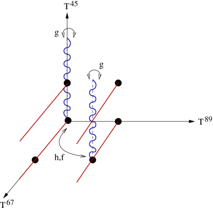
Figure 1: $D5_{1}$ and $D5_{2}$ brane configurations for the $w_{2}p_{3}$ model

As a consequence, the massless modes (or at times the full spectrum) exhibit enhanced supersymmetry. Figure 1 displays the brane configuration of the $w_{2}p_{3}$ model. The three axes refer to the three two-tori $T^{45}$, $T^{67}$ and $T^{89}$, and the $D5_{1}$ branes, drawn as wavy blue lines, occupy a pair of fixed tori, while the $D5_{2}$ branes, the solid red lines, occupy all the four fixed tori along the $Z^{2}$ direction. The $D5_{1}-D5_{1}$ configurations correspond to doublets of branes, associated to the pair of tori fixed by $g$ and interchanged by $f$ and $h$. As expected and as shown in Table 1, there is an $N=2$ supersymmetry associated to the $D5_{1}$ brane doublets together with an $N=4$ supersymmetry associated to the quartets of $D5_{2}$ branes.

3. Magnetic Deformations and Brane Transmutation

A uniform background magnetic field $H_{i}$ on the $i$-th torus is a monopole field, a $U(1)$ bundle with non-trivial transition functions gluing two local charts, whose consistency with particle dynamics requires a Dirac quantization condition

$$2\pi\alpha^{\prime}q_{i}H_{i}=\frac{k_{i}}{v_{i}}\qquad,$$ (3.1)

where $q_{i}$ is the $U(1)$-charge, $v_{i}$ is the volume of the torus and $k_{i}$ is an integer defining the (quantized) number of elementary fluxons or, equivalently, the Landau-level degeneracy. The background magnetic field couples solely to the open string ends through a boundary term in the action [30]. Thus, denoting with $q_{L}$ and $q_{R}$ the $U(1)$-charges at the two ends of the open strings and defining the total charge $Q=q_{L}+q_{R}$, one has to distinguish between “neutral”, $Q=0$, sectors and “charged”, $Q\neq 0$, ones. Charged open strings with $Q=\pm 1$ or $Q=\pm 2$ are characterized by oscillators whose frequencies are shifted according to

$$z_{i}=\frac{1}{\pi}[\ arctg(2\pi\alpha^{\prime}q_{L}H_{i})+arctg(2\pi\alpha^{\prime}q_{R}H_{i})\ ]\ .$$ (3.2)

Moreover, there is a Landau-level degeneracy that exactly amounts to the $k_{i}$ factor in eq. (3.1) and reflects the fact that the zero-modes along the two directions of the torus do not commute. Moreover, on a $Z_{N}$-orbifold the unit cell has a volume reduced by a factor $N$ with respect to the torus. As a result, the degeneracies of Landau levels should be multiples of $N$. For instance, $k_{i}$ are typically even on the $Z_{2}$-orbifold. However, a non-vanishing quantized NS-NS $B_{ab}$ could make some orbifold projections uneffective, thus allowing more choices for the $k_{i}$ [32]. On the other hand, neutral “dipole” strings with $q_{L}=-q_{R}$ ($Q=0$), have integer-mode frequencies, but the structure of their zero-modes is rather peculiar. Indeed, both momenta and windings are now allowed, but the effect of the magnetic field on this sector is simply to introduce rescalings in the momentum and winding lattices entering the one-loop annulus partition function. An analysis of the resulting projector along the tube shows that in the open one-loop channel the lattice sums over momenta and windings are indeed subjected to the “complex boosts”

$$m_{i}\rightarrow\frac{m_{i}}{\sqrt{1+(2\pi\alpha^{\prime}q_{i}H_{i})^{2}}}\ ,\quad n_{i}\rightarrow n_{i}\sqrt{1+(2\pi\alpha^{\prime}q_{i}H_{i})^{2}}\ .$$ (3.3)

Let us stress that a uniform Abelian magnetic field can be given a dual interpretation in terms of rotated branes [36]. In particular, after a T-duality along one of the two directions of one torus, the modified boundary conditions can be rephrased in terms of rotations of the corresponding $D$-branes by angles $\theta_{i}$ such that

$$\tan{\theta_{i}}=2\pi\alpha^{\prime}q_{i}H_{i}\quad.$$

The Dirac quantization condition in eq. (3.1) can then be interpreted as the requirement that the D-branes wrap exactly $k_{i}$-times the tori. Notice that we always normalize the electric charge of the open-strings in such a way that it corresponds to the elementary quantum. This is the reason why we can describe all spectra using just one integer $k_{i}$ for each two-torus or, in other words, setting to one the electric winding number of the corresponding $D$-branes.

Let us briefly review how these configurations manifest themselves in the orientifold of type IIB on a magnetized $(T^{2}\times T^{2})/Z_{2}$ [31]. This is a deformation of the six-dimensional $(T^{2}\times T^{2})/Z_{2}$ [2, 56] model, whose massless oriented closed spectrum is reported in Table 7 and comprises $N=(2,0)$ supergravity coupled to $21$ tensor multiplets, as expected for a singular limit of a $K_{3}$ compactification. The unoriented spectra, not affected by the constant magnetic backgrounds, are reported in table 8 and exhibit at zero mass $N=(1,0)$ supergravity modes coupled to hypermultiplets and tensor multiplets whose numbers depend upon the total rank $r$ of $B_{ab}$. In the open sector, the two magnetic fields $H_{1}$ and $H_{2}$ turned on inside the two $T^{2}$’s are aligned along the same $U(1)$ subgroup of the Chan-Paton gauge group. Generic fluxes of $H_{1}$ and $H_{2}$ produce the breaking of supersymmetry and the presence of Nielsen-Olesen instabilities, signaled by the appearance of tachyonic states. Absence of tachyons and supersymmetry can be attained choosing self-dual field configurations, that at the same time allow to compensate the non-vanishing instanton density with additional lower dimensional branes. As a result, the magnetized D9-branes mimic the behaviour of the D5-branes and couple to the R-R six-form, contributing to the tadpole cancellation conditions. This is the “brane transmutation” phenomenon, first described, in this context, in ref. [31] and linked there to the peculiar Wess-Zumino couplings in the D-brane actions [57]. There are several solutions, reported in Tables 9, 10, 11, 12 (see Appendix C for notations and conventions used in the Tables), depending on the $O$-plane configurations, or equivalently on the signs, analogous to the ones in Eq. (2.23), contained in the Möbius-strip amplitudes. In particular the R-R tadpole cancellation conditions and the resulting Chan-Paton gauge groups are shown in Table 9 for the models with complex charges and in Table 11 for the models with real charges. Moreover, the untwisted NS-NS tadpoles are related to the derivatives of the Born-Infeld action with respect to the untwisted moduli, while the twisted ones are associated with corresponding couplings in the effective Lagrangian, as in [31, 32]. The resulting open spectra, reported in Table 10 for complex charges and in Table 12 for real charges, can be easily recognized as deformations of the models without background magnetic fields [2, 56]. Several interesting facts, however, emerge from the analysis of Tables 10 and 12. First, there is an unusual rank reduction of the Chan-Paton gauge group. Second, some matter multiplets appear in multiple families, because of the degeneracy introduced by the Landau levels. Third, as already stressed the magnetized D9-branes behave exactly like D5-branes. This is particularly evident for the models without D5-branes, related for instance to the choice $r=0$, $k_{2}=k_{3}=2$, $d=0$, $n=12$ and $m=4$ in Table 10, and corresponds [58] to the fact that the D5-branes can be interpreted as instantons of vanishing size. So, in the presence of self-dual configurations of the internal magnetic fields, a stack of $2^{\frac{r}{2}}|k_{2}k_{3}|$ D5-branes is replaced by a “fat” instanton that invades the whole ten-dimensional space-time, in a transition related by $T$-duality [39] to the inverse small-instanton transition discussed in [58]. Finally, introducing antiself-dual configurations for the magnetic field, the magnetized $D9$-branes mimic anti-$D5$-branes [32]. Tachyons are again eliminated, but supersymmetry is broken at tree level in the open sector at the string scale or, better, is non-linearly realized in the anti $D5$-brane sector, as discussed in refs. [59, 60].

4. Magnetized Four-Dimensional Models

The four-dimensional models developed in refs. [20, 22] display $D9$ and $D5$ branes in their perturbative spectra, and are thus a natural arena to build consistent magnetized models sharing the qualitative features of the six-dimensional $T^{4}/Z_{2}$ model. As we shall see, their spectra exhibit rank reductions of the gauge groups and multiple matter families. In addition, as in the six-dimensional examples, there is the option of introducing pairs of magnetic fields aligned along the same $U(1)$ subgroup. This is allowed only if the undeformed model contains corresponding $O5$-planes orthogonal to the two magnetized directions, or, equivalently, if there are sources that add to the magnetized $D9$-branes in such a way as to compensate the R-R charge excess. We shall always introduce uniform Abelian background magnetic fields $(H_{2},H_{3})$ along the $(Z^{2},Z^{3})$ directions, thus requiring just the presence of $O5_{1}$-planes to balance the R-R charge excess of magnetized $D9$-branes and $D5_{1}$-branes.

If $D5$-branes whose world-volume invades coordinates longitudinal to the magnetized directions are also present, one obtains, as a bonus, chiral fermions. Chirality is connected on the one hand to the intersection of two sets of orthogonal $D5$-branes, and on the other to the chiral asymmetry in the “pure magnetic” sector. Moreover, the phenomenon of brane transmutation acquires in this setting its full-fledged form. Indeed, as stressed in Section 2, shift-orientifolds are characterized by the presence of multiplets of defocalized D5-branes. This implies, as mentioned before, that some of the D5-branes cannot be put on the same fixed tori but have to be distributed among the images interchanged by the action of some orbifold group elements. The magnetized D9-branes “remember” the localized distribution of the D5-branes they are mimicking. Indeed, although they invade the whole internal space, the centers of the corresponding classical Landau orbits organize themselves in multiplets that reflect the structure of the D5-branes.

4.1 Magnetized $Z_{2}\times Z_{2}$ Orientifolds

Let us begin the discussion of magnetic deformations by considering the “plain” $Z_{2}\times Z_{2}$ model with $\omega_{i}=1$ (for related examples in the language of intersecting $D$-brane models, see [39]). As stated in Section 2, the remaining models in Table 3 give rise to orientifolds with “brane supersymmetry breaking”, that, for brevity, will not be explicitly discussed here. However, in Section 5 we shall describe one class of orientifolds with “brane supersymmetry breaking” related to a class of $w_{2}p_{3}$ shift-orbifold models.

The closed string amplitudes, not affected by the introduction of constant background magnetic fields $H_{2}$ and $H_{3}$ along the $Z^{2}$ and $Z^{3}$ directions, as well as the $O$-plane content, are described in Section 2.2. In addition, the closed unoriented spectra are collected in Table 3. The annulus amplitude can be obtained using the techniques of [31], reviewed in Section 3, as a deformation of the annulus amplitudes of eq. (2.20). The result can be cast into the sum of the following three contributions (for notations and conventions see the Appendices)

$$\mathcal{A}_{(Q=0)} = \frac{1}{8}\biggl{\{}\bigl{(}N^{2}\ 2^{r-6}\ P_{1}(B_{1})P_{2}(B_{2})P_{3}(B_{3})+2m\bar{m}\ 2^{r-6}\ P_{1}(B_{1})\tilde{P}_{2}(B_{2})\tilde{P}_{3}(B_{3})$$ (4.1)

$$+ D_{1}^{2}\ 2^{r_{1}-2}\ P_{1}(B_{1})W_{2}W_{3}+D_{2}^{2}\ 2^{r_{2}-2}\ W_{1}P_{2}(B_{2})W_{3}$$

$$+ D_{3}^{2}\ 2^{r_{3}-2}\ W_{1}W_{2}P_{3}(B_{3})\bigr{)}T_{oo}(0;0;0)$$

$$+ 2^{\frac{r_{2}}{2}+\frac{r_{3}}{2}}\ T_{go}(0;0;0)\bigg{[}2ND_{1}\ 2^{r_{1}-2}\ P_{1}(B_{1})+2D_{2}D_{3}\ W_{1}\bigg{]}\,\Big{(}\frac{\eta}{\vartheta_{4}(0)}\Big{)}^{2}$$

$$+ 2^{\frac{r_{1}}{2}+\frac{r_{3}}{2}}\ T_{fo}(0;0;0)\bigg{[}2ND_{2}\ 2^{r_{2}-2}\ P_{2}(B_{2})+2D_{1}D_{3}\ W_{2}\bigg{]}\,\Big{(}\frac{\eta}{\vartheta_{4}(0)}\Big{)}^{2}$$

$$+ 2^{\frac{r_{1}}{2}+\frac{r_{2}}{2}}\ T_{ho}(0;0;0)\bigg{[}2ND_{3}\ 2^{r_{3}-2}\ P_{3}(B_{3})+2D_{1}D_{2}\ W_{3}\bigg{]}\,\Big{(}\frac{\eta}{\vartheta_{4}(0)}\Big{)}^{2}\biggl{\}}$$

for the zero-charge sectors,

$$\mathcal{A}_{(Q=1)} = \frac{1}{8}\biggl{\{}-2^{r-2}2mNT_{oo}(0;z_{2}\tau;z_{3}\tau)P_{1}(B_{1})\ \frac{k_{2}\eta}{\vartheta_{1}(z_{2}\tau)}\ \frac{k_{3}\eta}{\vartheta_{1}(z_{3}\tau)}$$ (4.2)

$$- 2^{r-2}2\bar{m}NT_{oo}(0;-z_{2}\tau;-z_{3}\tau)P_{1}(B_{1})\ \frac{k_{2}\eta}{\vartheta_{1}(-z_{2}\tau)}\ \frac{k_{3}\eta}{\vartheta_{1}(-z_{3}\tau)}$$

$$+ 2^{\frac{r_{2}}{2}+\frac{r_{3}}{2}}\ T_{go}(0;z_{2}\tau;z_{3}\tau)\bigg{[}2mD_{1}\ 2^{r_{1}-2}\ P_{1}(B_{1})\bigg{]}\,\frac{\eta}{\vartheta_{4}(z_{2}\tau)}\ \frac{\eta}{\vartheta_{4}(z_{3}\tau)}$$

$$+ 2^{\frac{r_{2}}{2}+\frac{r_{3}}{2}}\ T_{go}(0;-z_{2}\tau;-z_{3}\tau)\bigg{[}2\bar{m}D_{1}\ 2^{r_{1}-2}\ P_{1}(B_{1})\bigg{]}\,\frac{\eta}{\vartheta_{4}(-z_{2}\tau)}\ \frac{\eta}{\vartheta_{4}(-z_{3}\tau)}$$

$$+ 2^{\frac{r+r_{2}}{2}}\ T_{fo}(0;z_{2}\tau;z_{3}\tau)\bigg{[}-2imD_{2}\bigg{]}\,\frac{\eta}{\vartheta_{4}(0)}\ \frac{k_{2}\eta}{\vartheta_{1}(z_{2}\tau)}\ \frac{\eta}{\vartheta_{4}(z_{3}\tau)}$$

$$+ 2^{\frac{r+r_{2}}{2}}\ T_{fo}(0;-z_{2}\tau;-z_{3}\tau)\bigg{[}2i\bar{m}D_{2}\bigg{]}\,\frac{\eta}{\vartheta_{4}(0)}\ \frac{k_{2}\eta}{\vartheta_{1}(-z_{2}\tau)}\ \frac{\eta}{\vartheta_{4}(-z_{3}\tau)}$$

$$+ 2^{\frac{r+r_{3}}{2}}\ T_{ho}(0;z_{2}\tau;z_{3}\tau)\bigg{[}-2imD_{3}\bigg{]}\,\frac{\eta}{\vartheta_{4}(0)}\ \frac{\eta}{\vartheta_{4}(z_{2}\tau)}\ \frac{k_{3}\eta}{\vartheta_{1}(z_{3}\tau)}$$

$$+ 2^{\frac{r+r_{3}}{2}}\ T_{ho}(0;-z_{2}\tau;-z_{3}\tau)\bigg{[}2i\bar{m}D_{3}\bigg{]}\,\frac{\eta}{\vartheta_{4}(0)}\ \frac{\eta}{\vartheta_{4}(-z_{2}\tau)}\ \frac{k_{3}\eta}{\vartheta_{1}(-z_{3}\tau)}\biggl{\}}$$

for the charge-one sectors, and

$$\mathcal{A}_{(Q=2)} = \frac{1}{8}\biggl{\{}-2^{r-2}m^{2}T_{oo}(0;2z_{2}\tau;2z_{3}\tau)P_{1}(B_{1})\ \frac{2k_{2}\eta}{\vartheta_{1}(2z_{2}\tau)}\ \frac{2k_{3}\eta}{\vartheta_{1}(z_{3}\tau)}$$ (4.3)

$$- 2^{r-2}\bar{m}^{2}T_{oo}(0;-2z_{2}\tau;-2z_{3}\tau)P_{1}(B_{1})\ \frac{2k_{2}\eta}{\vartheta_{1}(-2z_{2}\tau)}\ \frac{2k_{3}\eta}{\vartheta_{1}(-2z_{3}\tau)}\biggl{\}}$$

for the total charge-two sectors. The Möbius amplitude can be obtained in a similar way from the undeformed case, distinguishing only the uncharged ($Q=0$) sector from the charged ($Q=2$) one, since the $Q=1$ sector is absent in $\mathcal{M}$ because of the oriented nature of the corresponding open-strings. Thus

$$\mathcal{M}_{(Q=0)}\!\! = \!\!\!-\frac{1}{8}\biggl{\{}\,\bigl{[}\,2^{\frac{r-6}{2}}\,N\,P_{1}(B_{1},\gamma_{\epsilon_{1}})\,P_{2}(B_{2},\gamma_{\epsilon_{2}})\,P_{3}(B_{3},\gamma_{\epsilon_{3}})$$

$$+ 2^{\frac{r_{1}-6}{2}}\,D_{1}\,P_{1}(B_{1},\gamma_{\epsilon_{1}})W_{2}(B_{2},\tilde{\gamma}_{\epsilon_{2}})W_{3}(B_{3},\tilde{\gamma}_{\epsilon_{3}})$$

$$+ 2^{\frac{r_{2}-6}{2}}\,D_{2}\,W_{1}(B_{1},\tilde{\gamma}_{\epsilon_{1}})P_{2}(B_{2},\gamma_{\epsilon_{2}})W_{3}(B_{3},\tilde{\gamma}_{\epsilon_{3}})$$

$$+ 2^{\frac{r_{3}-6}{2}}\,D_{3}\,W_{1}(B_{1},\tilde{\gamma}_{\epsilon_{1}})W_{2}(B_{2},\tilde{\gamma}_{\epsilon_{2}})P_{3}(B_{3},\gamma_{\epsilon_{3}})\,\bigr{]}\,\hat{T}_{oo}(0;0;0)$$

$$- \!\bigl{[}\,2^{\frac{r_{1}-2}{2}}\,(N\!+\!D_{1})P_{1}(B_{1},\gamma_{\epsilon_{1}})\!+\!2^{-1}\,(D_{2}\!+\!D_{3})W_{1}(B_{1},\tilde{\gamma}_{\epsilon_{1}})\bigr{]}\,\hat{T}_{og}(0;0;0)\left(\frac{2\hat{\eta}}{\hat{\theta_{2}}}\right)^{2}$$

$$- \!\bigl{[}\,2^{\frac{r_{2}-2}{2}}\,(N\!+\!D_{2})P_{2}(B_{2},\gamma_{\epsilon_{2}})\!+\!2^{-1}\,(D_{1}\!+\!D_{3})W_{2}(B_{2},\tilde{\gamma}_{\epsilon_{2}})\bigr{]}\,\hat{T}_{of}(0;0;0)\left(\frac{2\hat{\eta}}{\hat{\theta_{2}}}\right)^{2}$$

$$- \!\bigl{[}\,2^{\frac{r_{3}-2}{2}}\,(N\!+\!D_{3})P_{3}(B_{3},\gamma_{\epsilon_{3}})\!+\!2^{-1}\,(D_{1}\!+\!D_{2})W_{3}(B_{3},\tilde{\gamma}_{\epsilon_{3}})\bigr{]}\,\hat{T}_{oh}(0;0;0)\left(\frac{2\hat{\eta}}{\hat{\theta_{2}}}\right)^{2}\biggr{\}}\quad,$$

and

$$\mathcal{M}_{(Q=2)}\!\! = \!\!\ -\frac{1}{8}\biggl{\{}\,-2^{\frac{r-2}{2}}m\hat{T}_{oo}(0;2z_{2}\tau;2z_{3}\tau)\,P_{1}(B_{1},\gamma_{\epsilon_{1}})\,\frac{2k_{2}\hat{\eta}}{\hat{\vartheta}_{1}(2z_{2}\tau)}\frac{2k_{3}\hat{\eta}}{\hat{\vartheta}_{1}(2z_{3}\tau)}$$ (4.5)

$$- 2^{\frac{r-2}{2}}\bar{m}\hat{T}_{oo}(0;-2z_{2}\tau;-2z_{3}\tau)\,P_{1}(B_{1},\gamma_{\epsilon_{1}})\,\frac{2k_{2}\hat{\eta}}{\hat{\vartheta}_{1}(-2z_{2}\tau)}\frac{2k_{3}\hat{\eta}}{\hat{\vartheta}_{1}(-2z_{3}\tau)}$$

$$- 2^{\frac{r_{1}-2}{2}}m\hat{T}_{og}(0;2z_{2}\tau;2z_{3}\tau)\,P_{1}(B_{1},\gamma_{\epsilon_{1}})\,\frac{2\hat{\eta}}{\hat{\vartheta}_{2}(2z_{2}\tau)}\frac{2\hat{\eta}}{\hat{\vartheta}_{2}(2z_{3}\tau)}$$

$$- 2^{\frac{r_{1}-2}{2}}\bar{m}\hat{T}_{og}(0;-2z_{2}\tau;-2z_{3}\tau)\,P_{1}(B_{1},\gamma_{\epsilon_{1}})\,\frac{2\hat{\eta}}{\hat{\vartheta}_{2}(-2z_{2}\tau)}\frac{2\hat{\eta}}{\hat{\vartheta}_{2}(-2z_{3}\tau)}$$

$$+ i\,m\,2^{\frac{r_{2}}{2}}\,\hat{T}_{of}(0;2z_{2}\tau;2z_{3}\tau)\,\frac{2\hat{\eta}}{\hat{\vartheta}_{2}(0)}\,\frac{2k_{2}\hat{\eta}}{\hat{\vartheta}_{1}(2z_{2}\tau)}\frac{2\hat{\eta}}{\hat{\vartheta}_{2}(2z_{3}\tau)}$$

$$- i\,\bar{m}\,2^{\frac{r_{2}}{2}}\,\hat{T}_{of}(0;-2z_{2}\tau;-2z_{3}\tau)\,\frac{2\hat{\eta}}{\hat{\vartheta}_{2}(0)}\,\frac{2k_{2}\hat{\eta}}{\hat{\vartheta}_{1}(-2z_{2}\tau)}\frac{2\hat{\eta}}{\hat{\vartheta}_{2}(-2z_{3}\tau)}$$

$$+ i\,m\,2^{\frac{r_{3}}{2}}\,\hat{T}_{oh}(0;2z_{2}\tau;2z_{3}\tau)\,\frac{2\hat{\eta}}{\hat{\vartheta}_{2}(0)}\,\frac{2\hat{\eta}}{\hat{\vartheta}_{2}(2z_{2}\tau)}\frac{2k_{3}\hat{\eta}}{\hat{\vartheta}_{1}(2z_{3}\tau)}$$

$$- i\,\bar{m}\,2^{\frac{r_{3}}{2}}\,\hat{T}_{oh}(0;-2z_{2}\tau;-2z_{3}\tau)\,\frac{2\hat{\eta}}{\hat{\vartheta}_{2}(0)}\,\frac{2\hat{\eta}}{\hat{\vartheta}_{2}(-2z_{2}\tau)}\frac{2k_{3}\hat{\eta}}{\hat{\vartheta}_{1}(-2z_{3}\tau)}\biggr{\}}\quad.$$

These amplitudes describe the couplings of conventional $D9$ and $D5_{i}$ branes with an additional set of (magnetized) $D9$-branes. This natural interpretation is encoded into the four $o$, $g$, $f$ and $h$ projections, present in the ($Q=2$) sector of the Möbius amplitudes. The tadpole cancellation conditions may be extracted combining the transverse (tree) channel Klein-bottle amplitude of eq. (2.18) with the transverse annulus amplitudes

$$\tilde{\cal{A}} = \frac{2^{-5}}{8}\ \biggl{\{}\ [2^{r-6}v_{1}v_{2}v_{3}N^{2}W_{1}(B_{1})W_{2}(B_{2})W_{3}(B_{3})\ +\ \frac{v_{1}}{v_{2}v_{3}}\ 2^{r_{1}-2}\ D_{1}^{2}W_{1}(B_{1})P_{2}P_{3}$$ (4.6)

$$+ \frac{v_{2}}{v_{1}v_{3}}\ 2^{r_{2}-2}\ D_{2}^{2}P_{1}W_{2}(B_{2})P_{3}\ +\ \frac{v_{3}}{v_{1}v_{2}}\ 2^{r_{3}-2}\ D_{3}^{2}P_{1}P_{2}W_{3}(B_{3})$$

$$+ 2^{r-6}v_{1}v_{2}v_{3}\ 2m\bar{m}(1+q^{2}H_{2}^{2})(1+q^{2}H_{3}^{2})W_{1}(B_{1})\tilde{W_{2}}(B_{2})\tilde{W_{3}}(B_{3})\ ]\ T_{oo}(0;0;0)$$

$$+ 2^{r-2}\ 8\ N\ [mT_{oo}(0;z_{2};z_{3})+\bar{m}T_{oo}(0;-z_{2};-z_{3})]v_{1}W_{1}(B_{1})\ \frac{k_{2}\eta}{\vartheta_{1}(z_{2})}\frac{k_{3}\eta}{\vartheta_{1}(z_{3})}$$

$$+ 2^{r-2}\ 4\ [m^{2}T_{oo}(0;2z_{2};2z_{3})+\bar{m}^{2}T_{oo}(0;-2z_{2};-2z_{3})]v_{1}W_{1}(B_{1})\ \frac{2k_{2}\eta}{\vartheta_{1}(2z_{2})}\frac{2k_{3}\eta}{\vartheta_{1}(2z_{3})}$$

$$+ \ 2^{\frac{r_{2}}{2}+\frac{r_{3}}{2}}\ T_{og}(0;0;0)\Big{[}2^{r_{1}-2}\ 2ND_{1}v_{1}W_{1}(B_{1})+2D_{2}D_{3}\frac{P_{1}}{v_{1}}\Big{]}\ \frac{2\eta}{\vartheta_{2}(0)}\ \frac{2\eta}{\vartheta_{2}(0)}$$

$$+ \ 2^{\frac{r_{1}}{2}+\frac{r_{3}}{2}}\ T_{of}(0;0;0)\Big{[}2^{r_{2}-2}\ 2ND_{2}v_{2}W_{2}(B_{2})+2D_{1}D_{3}\frac{P_{2}}{v_{2}}\Big{]}\ \frac{2\eta}{\vartheta_{2}(0)}\ \frac{2\eta}{\vartheta_{2}(0)}$$

$$+ \ 2^{\frac{r_{1}}{2}+\frac{r_{2}}{2}}\ T_{oh}(0;0;0)\Big{[}2^{r_{3}-2}\ 2ND_{3}v_{3}W_{3}(B_{3})+2D_{1}D_{2}\frac{P_{3}}{v_{3}}\Big{]}\ \frac{2\eta}{\vartheta_{2}(0)}\ \frac{2\eta}{\vartheta_{2}(0)}$$

$$+ \ 2^{\frac{r_{2}}{2}+\frac{r_{3}}{2}}\ T_{og}(0;z_{2};z_{3})\Big{[}2^{r_{1}-2}\ 2mD_{1}v_{1}W_{1}(B_{1})\Big{]}\ \frac{2\eta}{\vartheta_{2}(z_{2})}\ \frac{2\eta}{\vartheta_{2}(z_{3})}$$

$$+ \ 2^{\frac{r_{2}}{2}+\frac{r_{3}}{2}}\ T_{og}(0;-z_{2};-z_{3})\Big{[}2^{r_{1}-2}\ 2\bar{m}D_{1}v_{1}W_{1}(B_{1})\Big{]}\ \frac{2\eta}{\vartheta_{2}(-z_{2})}\ \frac{2\eta}{\vartheta_{2}(-z_{3})}$$

$$+ \ 2^{\frac{r_{1}}{2}+\frac{r_{3}}{2}}\ T_{of}(0;z_{2};z_{3})\ 2mD_{2}\ \frac{2\eta}{\vartheta_{2}(0)}\ \frac{2k_{2}\eta}{\vartheta_{1}(z_{2})}\ \frac{2\eta}{\vartheta_{2}(z_{3})}$$

$$+ \ 2^{\frac{r_{1}}{2}+\frac{r_{3}}{2}}\ T_{of}(0;-z_{2};-z_{3})\ 2\bar{m}D_{2}\ \frac{2\eta}{\vartheta_{2}(0)}\ \frac{2k_{2}\eta}{\vartheta_{1}(-z_{2})}\ \frac{2\eta}{\vartheta_{2}(-z_{3})}$$

$$+ \ 2^{\frac{r_{1}}{2}+\frac{r_{2}}{2}}\ T_{oh}(0;z_{2};z_{3})\ 2mD_{3}\ \frac{2\eta}{\vartheta_{2}(0)}\ \frac{2\eta}{\vartheta_{2}(z_{2})}\ \frac{2k_{3}\eta}{\vartheta_{1}(z_{3})}$$

$$+ \ 2^{\frac{r_{1}}{2}+\frac{r_{2}}{2}}\ T_{oh}(0;-z_{2};-z_{3})\ 2\bar{m}D_{3}\ \frac{2\eta}{\vartheta_{2}(0)}\ \frac{2\eta}{\vartheta_{2}(-z_{2})}\ \frac{2k_{3}\eta}{\vartheta_{1}(-z_{3})}\ \biggr{\}}\quad,$$

and with the transverse Möbius amplitudes

$$\tilde{\cal{M}} = -\frac{2}{8}\ \biggl{\{}\ [\ 2^{\frac{r-6}{2}}\ N\ v_{1}v_{2}v_{3}\ W_{1}(B_{1},\gamma_{\epsilon_{1}})\ W_{2}(B_{2},\gamma_{\epsilon_{2}})\ W_{3}(B_{3},\gamma_{\epsilon_{3}})]\ \hat{T}_{oo}(0;0;0)$$ (4.7)

$$+ [\ 2^{\frac{r_{1}-6}{2}}\ \frac{v_{1}}{v_{2}v_{3}}\ D_{1}\ W_{1}(B_{1},\gamma_{\epsilon_{1}})\ P_{2}(B_{2},\tilde{\gamma}_{\epsilon_{2}})\ P_{3}(B_{3},\tilde{\gamma}_{\epsilon_{3}})\ ]\ \hat{T}_{oo}(0;0;0)$$

$$+ [\ 2^{\frac{r_{2}-6}{2}}\ \frac{v_{2}}{v_{1}v_{3}}\ D_{2}\ P_{1}(B_{1},\tilde{\gamma}_{\epsilon_{1}})\ W_{2}(B_{2},\gamma_{\epsilon_{2}})\ P_{3}(B_{3},\tilde{\gamma}_{\epsilon_{3}})\ ]\ \hat{T}_{oo}(0;0;0)$$

$$+ [\ 2^{\frac{r_{3}-6}{2}}\ \frac{v_{3}}{v_{1}v_{2}}\ D_{3}\ P_{1}(B_{1},\tilde{\gamma}_{\epsilon_{1}})\ P_{2}(B_{2},\tilde{\gamma}_{\epsilon_{2}})\ W_{3}(B_{3},\gamma_{\epsilon_{3}})\ ]\ \hat{T}_{oo}(0;0;0)$$

$$+ 2^{\frac{r_{1}}{2}+r_{2}+r_{3}-1}\ 4\ [\ m\hat{T}_{oo}(0;z_{2};z_{3})+\bar{m}\hat{T}_{oo}(0;-z_{2};-z_{3})\ ]\ v_{1}W_{1}(B_{1},\gamma_{\epsilon_{1}})\frac{k_{2}\hat{\eta}}{\hat{\vartheta}_{1}(z_{2})}\frac{k_{3}\hat{\eta}}{\hat{\vartheta}_{1}(z_{3})}$$

$$+ \hat{T}_{og}(0;0;0)\ [2^{\frac{r_{1}}{2}-1}(N+D_{1})v_{1}W_{1}(B_{1},\gamma_{\epsilon_{1}})\ +\ \frac{2^{-1}}{v_{1}}(D_{2}+D_{3})P_{1}(B_{1},\tilde{\gamma}_{\epsilon_{1}})]\ \frac{2\hat{\eta}}{\hat{\vartheta}_{2}(0)}\frac{2\hat{\eta}}{\hat{\vartheta}_{2}(0)}$$

$$+ \hat{T}_{of}(0;0;0)\ [2^{\frac{r_{2}}{2}-1}(N+D_{2})v_{2}W_{2}(B_{2},\gamma_{\epsilon_{2}})\ +\ \frac{2^{-1}}{v_{2}}(D_{1}+D_{3})P_{2}(B_{2},\tilde{\gamma}_{\epsilon_{2}})]\ \frac{2\hat{\eta}}{\hat{\vartheta}_{2}(0)}\frac{2\hat{\eta}}{\hat{\vartheta}_{2}(0)}$$

$$+ \hat{T}_{oh}(0;0;0)\ [2^{\frac{r_{3}}{2}-1}(N+D_{3})v_{3}W_{3}(B_{3},\gamma_{\epsilon_{3}})\ +\ \frac{2^{-1}}{v_{3}}(D_{1}+D_{2})P_{2}(B_{2},\tilde{\gamma}_{\epsilon_{2}})]\ \frac{2\hat{\eta}}{\hat{\vartheta}_{2}(0)}\frac{2\hat{\eta}}{\hat{\vartheta}_{2}(0)}$$

$$+ 2^{\frac{r_{1}}{2}-1}[\ m\hat{T}_{og}(0;z_{2};z_{3})+\bar{m}\hat{T}_{og}(0;-z_{2};-z_{3})\ ]\ v_{1}W_{1}(B_{1},\gamma_{\epsilon_{1}})\ \frac{2\hat{\eta}}{\hat{\vartheta}_{2}(z_{2})}\ \frac{2\hat{\eta}}{\hat{\vartheta}_{2}(z_{3})}$$

$$+ [\ m\hat{T}_{of}(0;z_{2};z_{3})-\bar{m}\hat{T}_{of}(0;-z_{2};-z_{3})\ ]\ \frac{2\hat{\eta}}{\hat{\vartheta}_{2}(0)}\ \frac{2k_{2}\hat{\eta}}{\hat{\vartheta}_{1}(z_{2})}\ \frac{2\hat{\eta}}{\hat{\vartheta}_{2}(z_{3})}$$

$$+ [\ m\hat{T}_{oh}(0;z_{2};z_{3})-\bar{m}\hat{T}_{oh}(0;-z_{2};-z_{3})\ ]\ \frac{2\hat{\eta}}{\hat{\vartheta}_{2}(0)}\ \frac{2\hat{\eta}}{\hat{\vartheta}_{2}(z_{2})}\ \frac{2k_{3}\hat{\eta}}{\hat{\vartheta}_{1}(z_{3})}\ \biggr{\}}\quad.$$

Apart from the $m=\bar{m}$ condition, automatic for the unitary gauge group selected by the magnetic background, all R-R tadpole cancellation conditions directly tied to four-dimensional non Abelian anomalies arise from the untwisted sector. After the charges are rescaled and parametrized in such a way that $N=2n$, $D_{i}=2d_{i}$ and $m\rightarrow 2m$, the resulting R-R conditions are as in Table 13, provided the signs $\gamma_{\epsilon}$ and $\tilde{\gamma}_{\epsilon}$ satisfy the same identities (2.22) of the undeformed case. The NS-NS tadpoles, canceled only at the supersymmetric $H_{2}=-H_{3}$ point, are related to the derivatives of the Born-Infeld action with respect to the moduli, exactly as in the six-dimensional case [31]. Several choices of gauge group are again allowed by the additional signs $\xi_{i}$ and $\eta_{i}$, in eq.(2.23). Introducing the combinations

$$2\rho_{\alpha,o}\ =\ a_{1}a_{2}a_{3}-a_{1}-a_{2}-a_{3}\ ,$$

$$2\rho_{\alpha,g}\ =\ a_{1}a_{2}a_{3}-a_{1}+a_{2}+a_{3}\ ,$$

$$2\rho_{\alpha,f}\ =\ a_{1}a_{2}a_{3}+a_{1}-a_{2}+a_{3}\ ,$$

$$2\rho_{\alpha,h}\ =\ a_{1}a_{2}a_{3}+a_{1}+a_{2}-a_{3}\ ,$$ (4.8)

where $a_{i}=\eta_{i}$ if $\alpha=n$ while $a_{i}=\eta_{i}$ but $a_{k}=\xi_{k},k\neq i$ if $\alpha=d_{i}$, the massless spectra are encoded in

$${\mathcal{A}}_{0}+{\mathcal{M}}_{0}\,=\,\tau_{oo}(0)\ \Big{[}\frac{n(n-\rho_{no})}{2}+\frac{d_{1}(d_{1}-\rho_{d_{1}o})}{2}+\frac{d_{2}(d_{2}-\rho_{d_{2}o})}{2}+\frac{d_{3}(d_{3}-\rho_{d_{3}o})}{2}+m\bar{m}\Big{]}$$ (4.9)

$$+ \tau_{og}(0)\Big{[}\frac{n(n-\rho_{ng})}{2}+\frac{d_{1}(d_{1}-\rho_{d_{1}g})}{2}+\frac{d_{2}(d_{2}-\rho_{d_{2}g})}{2}+\frac{d_{3}(d_{3}-\rho_{d_{3}g})}{2}+m\bar{m}\Big{]}$$

$$+ \tau_{oh}(0)\Big{[}\frac{n(n-\rho_{nh})}{2}+\frac{d_{1}(d_{1}-\rho_{d_{1}h})}{2}+\frac{d_{2}(d_{2}-\rho_{d_{2}h})}{2}+\frac{d_{3}(d_{3}-\rho_{d_{3}h})}{2}+m\bar{m}\Big{]}$$

$$+ \tau_{of}(0)\Big{[}\frac{n(n-\rho_{nf})}{2}+\frac{d_{1}(d_{1}-\rho_{d_{1}f})}{2}+\frac{d_{2}(d_{2}-\rho_{d_{2}f})}{2}+\frac{d_{3}(d_{3}-\rho_{d_{3}f})}{2}+m\bar{m}\Big{]}$$

$$+ \Big{[}\ \tau_{gh}(0)\ +\ \tau_{gf}(0)\ \Big{]}\ 2^{\frac{r_{2}}{2}+\frac{r_{3}}{2}}\ (nd_{1}+d_{2}d_{3})$$

$$+ \Big{[}\ \tau_{fg}(0)\ +\ \tau_{fh}(0)\ \Big{]}\ 2^{\frac{r_{1}}{2}+\frac{r_{3}}{2}}\ (nd_{2}+d_{1}d_{3})$$

$$+ \Big{[}\ \tau_{hg}(0)\ +\ \tau_{hf}(0)\ \Big{]}\ 2^{\frac{r_{1}}{2}+\frac{r_{2}}{2}}\ (nd_{3}+d_{1}d_{2})$$

$$+ \Big{[}\ \tau_{oh}(+)\ +\ \tau_{of}(+)\ \Big{]}\ 2^{r_{2}+r_{3}}\ |k_{2}k_{3}|\ nm\ +\ \Big{[}\ \tau_{oh}(-)\ +\ \tau_{of}(-)\ \Big{]}\ 2^{r_{2}+r_{3}}\ |k_{2}k_{3}|\ n\bar{m}$$

$$+ \Big{[}\ \tau_{gh}(+)\ +\ \tau_{gf}(+)\ \Big{]}\ 2^{\frac{r_{2}}{2}+\frac{r_{3}}{2}}\ md_{1}\ +\ \Big{[}\ \tau_{gh}(-)\ +\ \tau_{gf}(-)\ \Big{]}\ 2^{\frac{r_{2}}{2}+\frac{r_{3}}{2}}\ \bar{m}d_{1}$$

$$+ \Big{[}\ \tau_{fh}(+)\ \Big{]}\ 2^{\frac{r_{1}}{2}+\frac{r_{3}}{2}}\ md_{2}|k_{2}|\ +\ \Big{[}\ \tau_{fg}(-)\ \Big{]}2^{\frac{r_{1}}{2}+\frac{r_{3}}{2}}\bar{m}d_{2}|k_{2}|$$

$$+ \Big{[}\ \tau_{hg}(+)\ \Big{]}\ 2^{\frac{r_{1}}{2}+\frac{r_{2}}{2}}\ md_{3}|k_{3}|\ +\ \Big{[}\ \tau_{hf}(-)\ \Big{]}2^{\frac{r_{1}}{2}+\frac{r_{2}}{2}}\ \bar{m}d_{3}|k_{3}|$$

$$+ \Big{[}\ \tau_{oh}(2+)\ \Big{]}\ \frac{m(m-1)}{2}\ \Big{[}2^{r_{2}+r_{3}}2|k_{2}\,k_{3}|+2^{\frac{r_{2}+r_{3}}{2}}\eta_{1}|k_{2}\,k_{3}|+\eta_{1}+2^{\frac{r_{2}}{2}}|k_{2}|-2^{\frac{r_{3}}{2}}|k_{3}|\Big{]}$$

$$+ \Big{[}\ \tau_{oh}(2+)\ \Big{]}\ \frac{m(m+1)}{2}\ \Big{[}2^{r_{2}+r_{3}}2|k_{2}\,k_{3}|-2^{\frac{r_{2}+r_{3}}{2}}\eta_{1}|k_{2}\,k_{3}|-\eta_{1}-2^{\frac{r_{2}}{2}}|k_{2}|+2^{\frac{r_{3}}{2}}|k_{3}|\Big{]}$$

$$+ \Big{[}\ \tau_{of}(2+)\ \Big{]}\ \frac{m(m-1)}{2}\ \Big{[}2^{r_{2}+r_{3}}2|k_{2}\,k_{3}|+2^{\frac{r_{2}+r_{3}}{2}}\eta_{1}|k_{2}\,k_{3}|+\eta_{1}-2^{\frac{r_{2}}{2}}|k_{2}|+2^{\frac{r_{3}}{2}}|k_{3}|\Big{]}$$

$$+ \Big{[}\ \tau_{of}(2+)\ \Big{]}\ \frac{m(m+1)}{2}\ \Big{[}2^{r_{2}+r_{3}}2|k_{2}\,k_{3}|-2^{\frac{r_{2}+r_{3}}{2}}\eta_{1}|k_{2}\,k_{3}|-\eta_{1}+2^{\frac{r_{2}}{2}}|k_{2}|-2^{\frac{r_{3}}{2}}|k_{3}|\Big{]}$$

$$+ \Big{[}\ \tau_{of}(2-)\ \Big{]}\ \frac{\bar{m}(\bar{m}-1)}{2}\ \Big{[}2^{r_{2}+r_{3}}2|k_{2}\,k_{3}|+2^{\frac{r_{2}+r_{3}}{2}}\eta_{1}|k_{2}\,k_{3}|+\eta_{1}+2^{\frac{r_{2}}{2}}|k_{2}|-2^{\frac{r_{3}}{2}}|k_{3}|\Big{]}$$

$$+ \Big{[}\ \tau_{of}(2-)\ \Big{]}\ \frac{\bar{m}(\bar{m}+1)}{2}\ \Big{[}2^{r_{2}+r_{3}}2|k_{2}\,k_{3}|-2^{\frac{r_{2}+r_{3}}{2}}\eta_{1}|k_{2}\,k_{3}|-\eta_{1}-2^{\frac{r_{2}}{2}}|k_{2}|+2^{\frac{r_{3}}{2}}|k_{3}|\Big{]}$$

$$+ \Big{[}\ \tau_{oh}(2-)\ \Big{]}\ \frac{\bar{m}(\bar{m}-1)}{2}\ \Big{[}2^{r_{2}+r_{3}}2|k_{2}\,k_{3}|+2^{\frac{r_{2}+r_{3}}{2}}\eta_{1}|k_{2}\,k_{3}|+\eta_{1}-2^{\frac{r_{2}}{2}}|k_{2}|+2^{\frac{r_{3}}{2}}|k_{3}|\Big{]}$$

$$+ \Big{[}\ \tau_{oh}(2-)\ \Big{]}\ \frac{\bar{m}(\bar{m}+1)}{2}\ \Big{[}2^{r_{2}+r_{3}}2|k_{2}\,k_{3}|-2^{\frac{r_{2}+r_{3}}{2}}\eta_{1}|k_{2}\,k_{3}|-\eta_{1}+2^{\frac{r_{2}}{2}}|k_{2}|-2^{\frac{r_{3}}{2}}|k_{3}|\Big{]}\ ,$$

where $(0)$, $(\pm)$ and $(2\pm)$ are shorthand notations for the arguments $(0,0,0)$, $(0;\pm z_{2}\tau;\pm z_{3}\tau)$ and $(0;\pm 2z_{2}\tau;\pm 2z_{3}\tau)$, respectively, and the characters with non-vanishing arguments actually denote restrictions to their massless parts.

The resulting gauge groups are reported in Table 13, while the open unoriented spectra are displayed in Table 14. As expected from the previous discussion, chirality originates from two different sources. The first is the chiral asymmetry in the “pure magnetic” sector, due to the misalignment introduced by the combined action of magnetic backgrounds and orbifold projections on the Möbius amplitudes. The second is the coupling between magnetized $D9$-branes and $D5$-branes longitudinal to the magnetized complex directions, familiar from the $T$-dual picture, where chiral fermions live in a natural way at brane intersections [36]. Whenever potentially anomalous $U(1)$’s are present, they call for a generalization of the Dine-Seiberg-Witten mechanism [62], an option that, as in six dimensions [63], requires generalized Green-Schwarz couplings in the Ramond-Ramond sectors [64].

4.2 Magnetized $Z_{2}\times Z_{2}$ Shift-orientifolds

In this Section we describe the magnetized versions of the $Z_{2}\times Z_{2}$ shift-orientifolds introduced in [20] and reviewed in Section 2.3. As in the “plain” $Z_{2}\times Z_{2}$ models of Section 4.1, chiral matter can be obtained if open strings stretched between magnetized $D9$-branes and $D5$-branes longitudinal to the $Z^{2}$ and/or $Z^{3}$ directions are present. An inspection of Table 1 shows that the $p_{3}$, $w_{2}p_{3}$ and $w_{1}w_{2}p_{3}$ models are potentially chiral, while the remaining models are not.

The $p_{3}$ model requires a separate discussion, since in its undeformed version [20] it exhibits an $f$-twisted R-R tadpole condition, corresponding to the action of the $Z_{2}\times Z_{2}$ element that fixes the $T^{67}$-torus, one of the two along which we turn on background magnetic fluxes (see Table 16 for the unoriented closed spectra and Table 41 for the unoriented open spectra with complex Chan-Paton charges). This tadpole condition can no longer be satisfied if the background magnetic field is present, since some states are lifted in mass by a term depending solely on the field strength $H_{2}$ along $T^{67}$, rather than on the difference $H_{2}-H_{3}$ as in the case for the tadpole conditions coming from the untwisted or from the $g$-twisted sectors. The resulting models are thus anomalous as string vacua, because the magnetic deformations are, in the aforementioned sense, incompatible with the $p_{3}$ shift. The natural geometric interpretation of this phenomenon is as follows: the $p_{3}$ shift is introducing a net number of fractional branes [67] that, differently from what happens in the remaining models, are partly longitudinal and partly orthogonal to the magnetic fields carrying a non-vanishing twisted R-R charge, whose excess can be canceled only turning off the background magnetic field.

In the following we shall analyze the chiral and non-chiral examples with selfdual configurations of the magnetic field, i.e. at supersymmetric points, leaving to Section 5 the discussion of models with “brane supersymmetry breaking”.

4.2.1 $w_{2}p_{3}$ Models

Let us first analyze in detail the $w_{2}p_{3}$ class of orientifolds, that captures all interesting features of the models discussed in this paper. In the presence of the NS-NS two-form $B_{ab}$, the unoriented truncation of the closed spectrum is obtained adding to the halved torus amplitude the Klein-bottle amplitude

$${\cal K} = \frac{1}{8}\biggl{\{}\bigl{[}\ P_{1}\,P_{2}\,P_{3}\,+2^{-4}\,P_{1}\,W_{2}(B_{2})\,W_{3}(B_{3})\,$$ (4.10)

$$+ \!\!2^{-4}\,W_{1}(B_{1})\,P_{2}\,W_{3}(B_{3})$$

$$+ \!\!2^{-4}\,W_{1}(B_{1})\,(-1)^{n_{2}}W_{2}(B_{2})\,(-1)^{m_{3}}P_{3}\ \bigr{]}\,T_{oo}$$

$$+ \!\!2\times 16\,\bigl{[}\ 2^{-\frac{r_{2}}{2}-\frac{r_{3}}{2}}\,P_{1}\,T_{go}+2^{-\frac{r_{1}}{2}-\frac{r_{3}}{2}}\,P_{2}^{\frac{1}{2}}\,T_{fo}$$

$$+ \!\!2^{-\frac{r_{1}}{2}-\frac{r_{2}}{2}}\,2^{-2}\,W_{3}^{\frac{1}{2}}(B_{3})\,T_{ho}\ \bigr{]}\,\left(\frac{\eta}{\vartheta_{4}}\right)^{2}\biggr{\}}\quad.$$

The resulting massless unoriented closed spectra are reported in Table 17. The transverse-channel amplitude

$$\tilde{\cal K}_{0} = \frac{2^{5}}{8}\Biggl{\{}\ \left(\sqrt{v_{1}v_{2}v_{3}}+2^{-\frac{r_{2}}{2}-\frac{r_{3}}{2}}\sqrt{\frac{v_{1}}{v_{2}v_{3}}}+2^{-\frac{r_{1}}{2}-\frac{r_{3}}{2}}\sqrt{\frac{v_{2}}{v_{1}v_{3}}}\right)^{2}\tau_{oo}$$ (4.11)

$$+ \left(\sqrt{v_{1}v_{2}v_{3}}+2^{-\frac{r_{2}}{2}-\frac{r_{3}}{2}}\sqrt{\frac{v_{1}}{v_{2}v_{3}}}-2^{-\frac{r_{1}}{2}-\frac{r_{3}}{2}}\sqrt{\frac{v_{2}}{v_{1}v_{3}}}\right)^{2}\tau_{og}$$

$$+ \left(\sqrt{v_{1}v_{2}v_{3}}-2^{-\frac{r_{2}}{2}-\frac{r_{3}}{2}}\sqrt{\frac{v_{1}}{v_{2}v_{3}}}-2^{-\frac{r_{1}}{2}-\frac{r_{3}}{2}}\sqrt{\frac{v_{2}}{v_{1}v_{3}}}\right)^{2}\tau_{oh}$$

$$+ \left(\sqrt{v_{1}v_{2}v_{3}}-2^{-\frac{r_{2}}{2}-\frac{r_{3}}{2}}\sqrt{\frac{v_{1}}{v_{2}v_{3}}}+2^{-\frac{r_{1}}{2}-\frac{r_{3}}{2}}\sqrt{\frac{v_{2}}{v_{1}v_{3}}}\right)^{2}\tau_{of}\ \Biggr{\}}\quad$$

displays very neatly the presence of one conventional $O9$-plane and of the $O5_{1}$ and $O5_{2}$ planes, while the $O5_{3}$-plane of the $Z_{2}\times Z_{2}$-models in eq. (2.19) is no longer a fixed manifold of the combined orbifold and shifts, and is thus eliminated.

The annulus amplitude is more subtle. In the presence of $B_{ab}$, $H_{2}$ along $T^{67}$ and $H_{3}$ along $T^{89}$, it is again the sum of three contributions:

$$\mathcal{A}_{(Q=0)} = \frac{1}{8}\biggl{\{}\bigl{[}\frac{N^{2}}{2}\ 2^{r-6}\ P_{1}(B_{1})\ (\ P_{2}(B_{2})+P_{2}^{1/2}(B_{2})\ )\ P_{3}(B_{3})$$ (4.12)

$$+ \frac{2m\bar{m}}{2}\ 2^{r-6}\ P_{1}(B_{1})\ (\ \tilde{P}_{2}(B_{2})+\tilde{P}_{2}^{1/2}(B_{2})\ )\ \tilde{P}_{3}(B_{3})$$

$$+ \frac{D_{1}^{2}}{2}\ 2^{r_{1}-2}\ P_{1}(B_{1})W_{2}(\ W_{3}+W_{3}^{1/2}\ )$$

$$+ \frac{D_{2}^{2}}{4}\ 2^{r_{2}-2}\ W_{1}(\ P_{2}(B_{2})+P_{2}^{1/2}(B_{2})\ )\ (\ W_{3}+W_{3}^{1/2}\ )\bigr{]}T_{oo}(0;0;0)$$

$$+ 2^{r_{1}-2}\bigl{[}\frac{G^{2}}{2}+\frac{G_{1}^{2}}{2}+\frac{2m\bar{m}}{2}\bigr{]}T_{og}(0;0;0)\ P_{1}(B_{1})\Big{(}\frac{2\eta}{\vartheta_{2}(0)}\Big{)}^{2}$$

$$+ 2^{\frac{r_{1}}{2}+\frac{r_{3}}{2}}\ T_{go}(0;0;0)\ 2ND_{1}\ 2^{r_{1}-2}\ P_{1}(B_{1})\Big{(}\frac{\eta}{\vartheta_{4}(0)}\Big{)}^{2}$$

$$+ 2^{\frac{r_{1}}{2}+\frac{r_{3}}{2}}\ T_{gg}(0;0;0)\ 2GG_{1}\ 2^{r_{1}-2}\ P_{1}(B_{1})\Big{(}\frac{\eta}{\vartheta_{3}(0)}\Big{)}^{2}$$

$$+ 2^{\frac{r_{1}}{2}+\frac{r_{3}}{2}}\ T_{fo}(0;0;0)\ ND_{2}\ 2^{r_{2}-2}\ (\ P_{2}^{1/4}(B_{2})+P_{2}^{3/4}(B_{2})\ )\,\Big{(}\frac{\eta}{\vartheta_{4}(0)}\Big{)}^{2}$$

$$+ 2^{\frac{r_{1}}{2}+\frac{r_{2}}{2}}\ T_{ho}(0;0;0)\ 2^{r_{3}-2}D_{1}D_{2}\ (\ W_{3}^{1/4}+W_{3}^{3/4}\ )\,\Big{(}\frac{\eta}{\vartheta_{4}(0)}\Big{)}^{2}\biggl{\}}$$

for the $Q=0$ sectors,

$$\mathcal{A}_{(Q=1)} = \frac{1}{8}\biggl{\{}-2^{r-2}\,2\,m\,N\,T_{oo}(0;z_{2}\tau;z_{3}\tau)P_{1}(B_{1})\ \frac{k_{2}\eta}{\vartheta_{1}(z_{2}\tau)}\ \frac{k_{3}\eta}{\vartheta_{1}(z_{3}\tau)}$$ (4.13)

$$- 2^{r-2}\,2\,\bar{m}\,N\,T_{oo}(0;-z_{2}\tau;-z_{3}\tau)P_{1}(B_{1})\ \frac{k_{2}\eta}{\vartheta_{1}(-z_{2}\tau)}\ \frac{k_{3}\eta}{\vartheta_{1}(-z_{3}\tau)}$$

$$+ \ T_{og}(0;z_{2}\tau;z_{3}\tau)\bigg{[}\alpha_{mG}\,m\,G\ 2^{r_{1}-2}\ P_{1}(B_{1})\bigg{]}\,\frac{2\eta}{\vartheta_{2}(z_{2}\tau)}\ \frac{2\eta}{\vartheta_{2}(z_{3}\tau)}$$

$$+ \ T_{og}(0;-z_{2}\tau;-z_{3}\tau)\bigg{[}\bar{\alpha}_{mG}\,\bar{m}\,G\ 2^{r_{1}-2}\ P_{1}(B_{1})\bigg{]}\,\frac{2\eta}{\vartheta_{2}(-z_{2}\tau)}\ \frac{2\eta}{\vartheta_{2}(-z_{3}\tau)}$$

$$+ 2^{\frac{r_{2}}{2}+\frac{r_{3}}{2}}\ T_{go}(0;z_{2}\tau;z_{3}\tau)\bigg{[}2mD_{1}\ 2^{r_{1}-2}\ P_{1}(B_{1})\bigg{]}\,\frac{\eta}{\vartheta_{4}(z_{2}\tau)}\ \frac{\eta}{\vartheta_{4}(z_{3}\tau)}$$

$$+ 2^{\frac{r_{2}}{2}+\frac{r_{3}}{2}}\ T_{go}(0;-z_{2}\tau;-z_{3}\tau)\bigg{[}2\bar{m}D_{1}\ 2^{r_{1}-2}\ P_{1}(B_{1})\bigg{]}\,\frac{\eta}{\vartheta_{4}(-z_{2}\tau)}\ \frac{\eta}{\vartheta_{4}(-z_{3}\tau)}$$

$$+ 2^{\frac{r_{2}}{2}+\frac{r_{3}}{2}}\ T_{gg}(0;z_{2}\tau;z_{3}\tau)\bigg{[}\alpha_{mG_{1}}\ 2mG_{1}\ 2^{r_{1}-2}\ P_{1}(B_{1})\bigg{]}\,\frac{\eta}{\vartheta_{3}(z_{2}\tau)}\ \frac{\eta}{\vartheta_{3}(z_{3}\tau)}$$

$$+ 2^{\frac{r_{2}}{2}+\frac{r_{3}}{2}}\ T_{gg}(0;-z_{2}\tau;-z_{3}\tau)\bigg{[}\bar{\alpha}_{mG_{1}}\ 2\bar{m}G_{1}\ 2^{r_{1}-2}\ P_{1}(B_{1})\bigg{]}\,\frac{\eta}{\vartheta_{3}(-z_{2}\tau)}\ \frac{\eta}{\vartheta_{3}(-z_{3}\tau)}$$

$$+ 2^{\frac{r}{2}+\frac{r_{2}}{2}}\ T_{fo}(0;z_{2}\tau;z_{3}\tau)\bigg{[}-2imD_{2}\bigg{]}\,\frac{\eta}{\vartheta_{4}(0)}\ \frac{k_{2}\eta}{\vartheta_{1}(z_{2}\tau)}\ \frac{\eta}{\vartheta_{4}(z_{3}\tau)}$$

$$+ 2^{\frac{r}{2}+\frac{r_{2}}{2}}\ T_{fo}(0;-z_{2}\tau;-z_{3}\tau)\bigg{[}2i\bar{m}D_{2}\bigg{]}\,\frac{\eta}{\vartheta_{4}(0)}\ \frac{k_{2}\eta}{\vartheta_{1}(-z_{2}\tau)}\ \frac{\eta}{\vartheta_{4}(-z_{3}\tau)}\biggl{\}},$$

for the $Q=1$ sectors, and

$$\mathcal{A}_{(Q=2)} = \frac{1}{8}\biggl{\{}-2^{r-2}m^{2}T_{oo}(0;2z_{2}\tau;2z_{3}\tau)P_{1}(B_{1})\ \frac{2k_{2}\eta}{\vartheta_{1}(2z_{2}\tau)}\ \frac{k_{3}\eta}{2\vartheta_{1}(z_{3}\tau)}$$ (4.14)

$$- 2^{r-2}\bar{m}^{2}T_{oo}(0;-2z_{2}\tau;-2z_{3}\tau)P_{1}(B_{1})\ \frac{k_{2}\eta}{\vartheta_{1}(-2z_{2}\tau)}\ \frac{k_{3}\eta}{\vartheta_{1}(-2z_{3}\tau)}$$

$$+ 2^{r_{1}-2}\alpha_{m^{2}}\ \frac{m^{2}}{2}T_{og}(0;2z_{2}\tau;2z_{3}\tau)P_{1}(B_{1})\ \frac{2\eta}{\vartheta_{2}(2z_{2}\tau)}\ \frac{2\eta}{\vartheta_{2}(2z_{3}\tau)}$$

$$+ 2^{r_{1}-2}\bar{\alpha}_{m^{2}}\ \frac{\bar{m}^{2}}{2}T_{og}(0;-2z_{2}\tau;-2z_{3}\tau)P_{1}(B_{1})\ \frac{2\eta}{\vartheta_{2}(-2z_{2}\tau)}\ \frac{2\eta}{\vartheta_{2}(-2z_{3}\tau)}\biggl{\}}.$$

for the $Q=2$ sectors, where the magnetized Chan-Paton charge multiplicity is denoted by $m$. The coefficients $\alpha_{mG}$, $\bar{\alpha}_{mG}$, $\alpha_{mG_{1}}$, $\bar{\alpha}_{mG_{1}}$, $\alpha_{m^{2}}$ and $\bar{\alpha}_{m^{2}}$ must be chosen in such a way that the annulus amplitudes become real. The Möbius amplitude can be deduced in a similar way from the undeformed case, adding to the uncharged ($Q=0$) contributions the charged ($Q=2$) ones. The result is

$$\mathcal{M}_{(Q=0)} = -\frac{1}{8}\biggl{\{}\,\bigl{[}\,2^{\frac{r-6}{2}}\,N\,P_{1}(B_{1},\gamma_{\epsilon_{1}})\,P_{2}(B_{2},\gamma_{\epsilon_{2}})\,P_{3}(B_{3},\gamma_{\epsilon_{3}})$$ (4.15)

$$+ 2^{\frac{r_{1}-6}{2}}\,D_{1}\,P_{1}(B_{1},\gamma_{\epsilon_{1}})W_{2}(B_{2},\tilde{\gamma}_{\epsilon_{2}})W_{3}(B_{3},\tilde{\gamma}_{\epsilon_{3}})$$

$$+ 2^{\frac{r_{2}-6}{2}}\,D_{2}\,W_{1}(B_{1},\tilde{\gamma}_{\epsilon_{1}})P_{2}(B_{2},\gamma_{\epsilon_{2}})W_{3}(B_{3},\tilde{\gamma}_{\epsilon_{3}})\bigr{]}\,\hat{T}_{oo}(0;0;0)$$

$$- \!\bigl{[}\,2^{\frac{r_{1}-2}{2}}\,(N\!+\!D_{1})P_{1}(B_{1},\gamma_{\epsilon_{1}})\bigr{]}\,\hat{T}_{og}(0;0;0)\left(\frac{2\hat{\eta}}{\hat{\theta_{2}}}\right)^{2}$$

$$- \!\bigl{[}\,2^{\frac{r_{2}-2}{2}}\,(N\!+\!D_{2})P_{2}^{1/2}(B_{2},\gamma_{\epsilon_{2}})\bigr{]}\,\hat{T}_{of}(0;0;0)\left(\frac{2\hat{\eta}}{\hat{\theta_{2}}}\right)^{2}$$

$$- \!\bigl{[}\,2^{-1}\,(D_{1}\!+\!D_{2})W_{3}(B_{3},\tilde{\gamma}_{\epsilon_{3}})\bigr{]}\,\hat{T}_{oh}(0;0;0)\left(\frac{2\hat{\eta}}{\hat{\theta_{2}}}\right)^{2}\ \biggr{\}}\quad,$$

and

$$\mathcal{M}_{(Q=2)} = -\frac{1}{8}\biggl{\{}\,-2^{\frac{r-2}{2}}m\hat{T}_{oo}(0;2z_{2}\tau;2z_{3}\tau)\,P_{1}(B_{1},\gamma_{\epsilon_{1}})\,\frac{2k_{2}\hat{\eta}}{\hat{\vartheta}_{1}(2z_{2}\tau)}\frac{2k_{3}\hat{\eta}}{\hat{\vartheta}_{1}(2z_{3}\tau)}$$ (4.16)

$$- 2^{\frac{r-2}{2}}\bar{m}\hat{T}_{oo}(0;-2z_{2}\tau;-2z_{3}\tau)\,P_{1}(B_{1},\gamma_{\epsilon_{1}})\,\frac{2k_{2}\hat{\eta}}{\hat{\vartheta}_{1}(-2z_{2}\tau)}\frac{2k_{3}\hat{\eta}}{\hat{\vartheta}_{1}(-2z_{3}\tau)}$$

$$- 2^{\frac{r_{1}-2}{2}}m\hat{T}_{og}(0;2z_{2}\tau;2z_{3}\tau)\,P_{1}(B_{1},\gamma_{\epsilon_{1}})\,\frac{2\hat{\eta}}{\hat{\vartheta}_{2}(2z_{2}\tau)}\frac{2\hat{\eta}}{\hat{\vartheta}_{2}(2z_{3}\tau)}$$

$$- 2^{\frac{r_{1}-2}{2}}\bar{m}\hat{T}_{og}(0;-2z_{2}\tau;-2z_{3}\tau)\,P_{1}(B_{1},\gamma_{\epsilon_{1}})\,\frac{2\hat{\eta}}{\hat{\vartheta}_{2}(-2z_{2}\tau)}\frac{2\hat{\eta}}{\hat{\vartheta}_{2}(-2z_{3}\tau)}$$

$$- 2^{\frac{r_{2}}{2}}im\hat{T}_{of}(0;2z_{2}\tau;2z_{3}\tau)\,\frac{2\hat{\eta}}{\hat{\vartheta}_{2}(0)}\,\frac{2k_{2}\hat{\eta}}{\hat{\vartheta}_{1}(2z_{2}\tau)}\frac{2\hat{\eta}}{\hat{\vartheta}_{2}(2z_{3}\tau)}$$

$$- 2^{\frac{r_{2}}{2}}(-i)\bar{m}\hat{T}_{of}(0;-2z_{2}\tau;-2z_{3}\tau)\,\frac{2\hat{\eta}}{\hat{\vartheta}_{2}(0)}\,\frac{2k_{2}\hat{\eta}}{\hat{\vartheta}_{1}(-2z_{2}\tau)}\frac{2\hat{\eta}}{\hat{\vartheta}_{2}(-2z_{3}\tau)}\biggr{\}}\quad.$$

In order to analyze in some detail the tadpole cancellation conditions, it is worth displaying the transverse (tree) channel amplitudes. The annulus part comprises untwisted and twisted terms

$$\tilde{\cal{A}}=\tilde{\cal{A}}^{U}+\tilde{\cal{A}}^{T}\qquad,$$

where

$$\tilde{\cal{A}}^{U} = \frac{2^{-5}}{8}\ \biggl{\{}\ [2^{r-6}v_{1}v_{2}v_{3}\frac{N^{2}}{2}W_{1}(B_{1})(W_{2}(B_{2})+(-1)^{n_{2}}W_{2}(B_{2}))W_{3}(B_{3})$$

$$+ \ \frac{v_{1}}{v_{2}v_{3}}\ 2^{r_{1}-2}\ \frac{D_{1}^{2}}{2}W_{1}(B_{1})P_{2}(P_{3}+(-1)^{m_{3}}P_{3})$$

$$+ \frac{v_{2}}{v_{1}v_{3}}\ 2^{r_{2}-2}\ \frac{D_{2}^{2}}{4}P_{1}(W_{2}(B_{2})+(-1)^{n_{2}}W_{2}(B_{2}))(P_{3}+(-1)^{m_{3}}P_{3})$$

$$+ 2^{r-6}v_{1}v_{2}v_{3}\ \frac{2m\bar{m}}{2}(1+q^{2}H_{2}^{2})(1+q^{2}H_{3}^{2})W_{1}(B_{1})(\tilde{W_{2}}(B_{2})$$

$$+ (-1)^{n_{2}}\tilde{W_{2}}(B_{2}))\tilde{W_{3}}(B_{3})\ ]\ T_{oo}(0;0;0)$$

$$+ \ 2^{\frac{r_{2}}{2}+\frac{r_{3}}{2}}\ \Big{[}2^{r_{1}-2}\ 2ND_{1}v_{1}W_{1}(B_{1})\Big{]}\ T_{og}(0;0;0)\ \frac{2\eta}{\vartheta_{2}(0)}\ \frac{2\eta}{\vartheta_{2}(0)}$$

$$+ \ 2^{\frac{r_{1}}{2}+\frac{r_{3}}{2}}\ \Big{[}2^{r_{2}-2}\ ND_{2}v_{2}((i)^{n_{2}}W_{2}(B_{2})+(-i)^{n_{2}}W_{2}(B_{2}))\Big{]}\ T_{of}(0;0;0)\ \frac{2\eta}{\vartheta_{2}(0)}\ \frac{2\eta}{\vartheta_{2}(0)}$$

$$+ \ 2^{\frac{r_{1}}{2}+\frac{r_{2}}{2}}\ \Big{[}D_{1}D_{2}\frac{1}{v_{3}}((i)^{m_{3}}P_{3}+(-i)^{m_{3}}P_{3})\Big{]}\ T_{oh}(0;0;0)\ \frac{2\eta}{\vartheta_{2}(0)}\ \frac{2\eta}{\vartheta_{2}(0)}$$

$$+ 2^{r-2}\ 8\ N\ v_{1}W_{1}(B_{1})[mT_{oo}(0;z_{2};z_{3})+\bar{m}T_{oo}(0;-z_{2};-z_{3})]\ \frac{k_{2}\eta}{\vartheta_{1}(z_{2})}\frac{k_{3}\eta}{\vartheta_{1}(z_{3})}$$

$$+ \ 2^{\frac{r}{2}+\frac{r_{1}}{2}-2}\ 2D_{1}v_{1}W_{1}(B_{1})\Big{[}mT_{og}(0;z_{2};z_{3})+\bar{m}T_{og}(0;-z_{2};-z_{3})\Big{]}\ \frac{2\eta}{\vartheta_{2}(z_{2})}\ \frac{2\eta}{\vartheta_{2}(z_{3})}$$

$$+ \ 2^{\frac{r_{2}}{2}+\frac{r_{3}}{2}}\ \Big{[}2^{r_{1}-2}\ 2\bar{m}D_{1}v_{1}W_{1}(B_{1})\Big{]}\ T_{og}(0;-z_{2};-z_{3})\ \frac{2\eta}{\vartheta_{2}(-z_{2})}\ \frac{2\eta}{\vartheta_{2}(-z_{3})}$$

$$+ \ 2^{\frac{r}{2}+\frac{r_{2}}{2}}\ \ 2mD_{2}\ T_{of}(0;z_{2};z_{3})\ \frac{2\eta}{\vartheta_{2}(0)}\ \frac{2k_{2}\eta}{\vartheta_{1}(z_{2})}\ \frac{2\eta}{\vartheta_{2}(z_{3})}$$

$$- \ 2^{\frac{r}{2}+\frac{r_{2}}{2}}\ \ 2\bar{m}D_{2}\ T_{of}(0;-z_{2};-z_{3})\ \frac{2\eta}{\vartheta_{2}(0)}\ \frac{2k_{2}\eta}{\vartheta_{1}(-z_{2})}\ \frac{2\eta}{\vartheta_{2}(-z_{3})}$$

$$+ 2^{r-2}\ 4\ v_{1}W_{1}(B_{1})\ [m^{2}T_{oo}(0;2z_{2};2z_{3})+\bar{m}^{2}T_{oo}(0;-2z_{2};-2z_{3})]\ \frac{2k_{2}\eta}{\vartheta_{1}(2z_{2})}\frac{2k_{3}\eta}{\vartheta_{1}(2z_{3})}\ \biggr{\}}\quad,$$

and

$$\tilde{\cal{A}}^{T} = \frac{2^{-5}}{8}\ \biggl{\{}\ 2^{r_{1}-2}\ 16\ v_{1}W_{1}(B_{1})\Big{[}\frac{G^{2}}{2}+\frac{{G^{2}}_{1}}{2}\frac{2m\bar{m}}{2}\Big{]}\ T_{go}(0;0;0)\ \frac{\eta}{\vartheta_{4}(0)}\ \frac{\eta}{\vartheta_{4}(0)}$$ (4.18)

$$- \ 2^{\frac{r}{2}+\frac{r_{1}}{2}-2}\ v_{1}W_{1}(B_{1})\ 8\ GG_{1}\ T_{gg}(0;0;0)\ \frac{\eta}{\vartheta_{3}(0)}\ \frac{\eta}{\vartheta_{3}(0)}$$

$$+ 2^{r_{1}-2}\ 16\ G\ v_{1}W_{1}(B_{1})\Big{[}\ \alpha_{mG}mT_{go}(0;z_{2};z_{3})+\bar{\alpha}_{mG}\bar{m}T_{go}(0;-z_{2};-z_{3})\Big{]}\ \frac{\eta}{\vartheta_{4}(z_{2})}\ \frac{\eta}{\vartheta_{4}(z_{3})}$$

$$- \ 2^{\frac{r}{2}+\frac{r_{1}}{2}-2}\ 8\ G_{1}\ v_{1}\ W_{1}(B_{1})\ \Big{[}\ \alpha_{mG_{1}}\ m\ T_{gg}(0;z_{2};z_{3})$$

$$+ \bar{\alpha}_{mG_{1}}\ \bar{m}\ T_{gg}(0;-z_{2};-z_{3})\ \Big{]}\ \frac{\eta}{\vartheta_{3}(z_{2})}\ \frac{\eta}{\vartheta_{3}(z_{3})}$$

$$+ 2^{r_{1}-2}\ 8\ v_{1}\ W_{1}(B_{1})\ \Big{[}\ \alpha_{m^{2}}\ m^{2}\ T_{go}(0;2z_{2};2z_{3})$$

$$+ \bar{\alpha}_{m^{2}}\ \bar{m}^{2}\ T_{go}(0;-2z_{2};-2z_{3})\ \Big{]}\ \frac{\eta}{\vartheta_{4}(2z_{2})}\ \frac{\eta}{\vartheta_{4}(2z_{3})}\ \biggr{\}}\quad.$$

This is to be contrasted with the transverse Möbius amplitude, that contains only untwisted contributions

$$\tilde{\cal{M}} = -\frac{2}{8}\ \biggl{\{}\ \Big{[}\ 2^{\frac{r-6}{2}}\ N\ v_{1}v_{2}v_{3}\ W^{e}_{1}(B_{1},\gamma_{\epsilon_{1}})\ W^{e}_{2}(B_{2},\gamma_{\epsilon_{2}})\ W^{e}_{3}(B_{3},\gamma_{\epsilon_{3}})$$ (4.19)

$$+ 2^{\frac{r_{1}-6}{2}}\ \frac{v_{1}}{v_{2}v_{3}}\ D_{1}\ W^{e}_{1}(B_{1},\gamma_{\epsilon_{1}})\ P^{e}_{2}(B_{2},\tilde{\gamma}_{\epsilon_{2}})\ P^{e}_{3}(B_{3},\tilde{\gamma}_{\epsilon_{3}})$$

$$+ 2^{\frac{r_{2}-6}{2}}\ \frac{v_{2}}{v_{1}v_{3}}\ D_{2}\ P^{e}_{1}(B_{1},\tilde{\gamma}_{\epsilon_{1}})\ W^{e}_{2}(B_{2},\gamma_{\epsilon_{2}})\ P^{e}_{3}(B_{3},\tilde{\gamma}_{\epsilon_{3}})\ \Big{]}\ \hat{T}_{oo}(0;0;0)$$

$$+ 2^{\frac{r_{1}}{2}-1}\ (N+D_{1})\ v_{1}\ W^{e}_{1}(B_{1},\gamma_{\epsilon_{1}})\ \hat{T}_{og}(0;0;0)\ \frac{2\hat{\eta}}{\hat{\vartheta}_{2}(0)}\ \frac{2\hat{\eta}}{\hat{\vartheta}_{2}(0)}$$

$$+ 2^{\frac{r_{2}}{2}-1}\ (N+D_{2})\ v_{2}\ W^{e}_{2}(B_{2},\gamma_{\epsilon_{2}})\ \hat{T}_{of}(0;0;0)\ \frac{2\hat{\eta}}{\hat{\vartheta}_{2}(0)}\ \frac{2\hat{\eta}}{\hat{\vartheta}_{2}(0)}$$

$$+ \frac{2^{-1}}{v_{3}}\ (D_{1}+D_{2})\ \phi^{B_{3}}\ P^{e}_{3}(B_{3},\tilde{\gamma}_{\epsilon_{3}})\ \hat{T}_{oh}(0;0;0)\ \frac{2\hat{\eta}}{\hat{\vartheta}_{2}(0)}\ \frac{2\hat{\eta}}{\hat{\vartheta}_{2}(0)}$$

$$+ 2^{\frac{r}{2}-1}\ 4\ v_{1}W^{e}_{1}(B_{1},\gamma_{\epsilon_{1}})\ [\ m\hat{T}_{oo}(0;z_{2};z_{3})+\bar{m}\hat{T}_{oo}(0;-z_{2};-z_{3})\ ]\ \frac{k_{2}\hat{\eta}}{\hat{\vartheta}_{1}(z_{2})}\frac{k_{3}\hat{\eta}}{\hat{\vartheta}_{1}(z_{3})}$$

$$+ 2^{\frac{r_{1}}{2}-1}\ v_{1}W^{e}_{1}(B_{1},\gamma_{\epsilon_{1}})\ [\ m\hat{T}_{og}(0;z_{2};z_{3})+\bar{m}\hat{T}_{og}(0;-z_{2};-z_{3})\ ]\ \frac{2\hat{\eta}}{\hat{\vartheta}_{2}(z_{2})}\ \frac{2\hat{\eta}}{\hat{\vartheta}_{2}(z_{3})}$$

$$+ 2^{\frac{r_{2}}{2}}\ m\ \hat{T}_{of}(0;z_{2};z_{3})\ \frac{2\hat{\eta}}{\hat{\vartheta}_{2}(0)}\ \frac{2k_{2}\hat{\eta}}{\hat{\vartheta}_{1}(z_{2})}\ \frac{2\hat{\eta}}{\hat{\vartheta}_{2}(z_{3})}$$

$$- 2^{\frac{r_{2}}{2}}\ \bar{m}\ \hat{T}_{of}(0;-z_{2};-z_{3})\ \frac{2\hat{\eta}}{\hat{\vartheta}_{2}(0)}\ \frac{2k_{2}\hat{\eta}}{\hat{\vartheta}_{1}(-z_{2})}\ \frac{2\hat{\eta}}{\hat{\vartheta}_{2}(-z_{3})}\biggr{\}}\quad,$$

where $\phi^{B_{3}}$ is a suitable phase that depends on the rank of $B_{ab}$, not directly relevant for our discussion. The untwisted tadpole cancellation conditions are related to the superposition of $\tilde{{\cal K}}$, $\tilde{{\cal A}}$ and $\tilde{{\cal M}}$, and can be obtained as follows. The residues corresponding to the R-R part of the $\tau_{0\alpha}$ character are

$$\!\!\!\!\!\!\sqrt{v_{1}v_{2}v_{3}}\,\left\{\,2^{\frac{r}{2}}\,\left[\,N+(m+\bar{m})(1-4\pi^{2}{\alpha^{\prime}}^{2}q^{2}H_{2}H_{3})+(m-\bar{m})\ 8i\pi^{2}{\alpha^{\prime}}^{2}q^{2}(H_{2}+H_{3})\,\right]-32\,\right\}$$ (4.20)

$$+ \lambda_{1\alpha}\,\sqrt{\frac{v_{1}}{v_{2}v_{3}}}\ \left[\,2^{\frac{r_{1}}{2}}D_{1}\ -\ 32\,2^{-\frac{r_{2}+r_{3}}{2}}\,\right]\ +\ \lambda_{2\alpha}\,\sqrt{\frac{v_{2}}{v_{1}v_{3}}}\ \left[\,2^{\frac{r_{2}}{2}}D_{2}\ -\ 32\,2^{-\frac{r_{1}+r_{3}}{2}}\,\right]\,=\,0,$$

together with the complex conjugates, where $\lambda_{1\alpha}$ is $+1$ for $\alpha=o,g$ and is $-1$ for $\alpha=h,f$ while $\lambda_{2\alpha}$ is $+1$ for $\alpha=o,f$ and is $-1$ for $\alpha=g,h$. In order to obtain eqs. (4.20), the conditions in (2.22) for the signs $\gamma_{\epsilon}$ and $\tilde{\gamma}_{\epsilon}$ must be used, and, in order to ensure the vanishing of the imaginary part the numerical constraint, $m=\bar{m}$ must also be enforced. Using the Dirac quantization condition in eq. (3.1), it is interesting to notice that the magnetized $D9$-branes contribute not only to the tadpole of the R-R ten-form, but also to the tadpole of the R-R six-form. As in the six-dimensional examples, this signals the phenomenon of brane transmutation. In particular, disentangling the diverse contributions, one obtains

$$\sqrt{v_{1}v_{2}v_{3}}\,\left[\,2^{\frac{r}{2}}\,(\,N+m+\bar{m})\,\right]\ =\ \sqrt{v_{1}v_{2}v_{3}}\ 32$$ (4.21)

for the $D9$-brane sector,

$$\sqrt{\frac{v_{1}}{v_{2}v_{3}}}\ \left[\,2^{\frac{r_{1}}{2}}D_{1}\ +2^{\frac{r}{2}}\,|k_{2}k_{3}|\,(m+\bar{m})\,\right]\ =\ \sqrt{\frac{v_{1}}{v_{2}v_{3}}}\,\left[\,32\,2^{-\frac{r_{2}+r_{3}}{2}}\,\right]$$ (4.22)

for the $D5_{1}$-brane sector and

$$\sqrt{\frac{v_{2}}{v_{1}v_{3}}}\ \left[\,2^{\frac{r_{2}}{2}}D_{2}\right]\ =\ \sqrt{\frac{v_{2}}{v_{1}v_{3}}}\,\left[\,32\,2^{-\frac{r_{1}+r_{3}}{2}}\,\right]$$ (4.23)

for the $D5_{2}$-brane sector.

The twisted tadpole conditions determine the nature of the allowed Chan-Paton charges. There are two options, that result in complex or real Chan-Paton charges. In the complex case, one must choose

$$\alpha_{mG}=-\bar{\alpha}_{mG}=\alpha_{mG_{1}}=-\bar{\alpha}_{mG_{1}}\ =\ i\quad;\qquad\alpha_{m^{2}}=\bar{\alpha}_{m^{2}}\ =\ -1\quad,$$

and the tadpole cancellation condition can be written

$$(8-2^{r-r_{1}+1})\ [\,G+im-i\bar{m}\,]^{2}+2\ [\,2\,G_{1}+2^{\frac{r-r_{1}}{2}}\,(\,G+im-i\bar{m}\,)\,]^{2}=0\quad,$$ (4.24)

while the real charges are determined by the choice

$$\alpha_{mG}=-\bar{\alpha}_{mG}=\alpha_{mG_{1}}=-\bar{\alpha}_{mG_{1}}=\alpha_{m^{2}}=\bar{\alpha}_{m^{2}}\ =\ 1,$$

and the corresponding tadpole cancellation condition can be written in the form

$$(8-2^{r-r_{1}+1})\ [\,G+m+\bar{m}\,]^{2}+2\ [\,2\,G_{1}+2^{\frac{r-r_{1}}{2}}\,(\,G+m+\bar{m}\,)\,]^{2}=0\quad.$$ (4.25)

The analysis of the open spectra is very similar to the one in Section 2, and therefore we shall not repeat it here. With complex charges, after the choice of signs in eq. (2.23), one has to fix

$$\xi_{2}\ \xi_{3}=\eta_{2}\ \eta_{3}\ =\ 1\quad,$$ (4.26)

while $\xi_{1}$ and $\eta_{1}$ are free signs. In order to obtain amplitudes with a proper particle interpretation, the magnetic charges must be rescaled by a factor of two, and a suitable parametrization of the Chan-Paton multiplicities is

$$N = \ 2\ (\ n\ +\ \bar{n}\ )\quad,\qquad G\ =\ 2\ i\ (\ n\ -\ \bar{n}\ )\quad;$$

$$D_{1} = 2\ (\ d\ +\ \bar{d}\ )\quad,\qquad G_{1}\ =\ 2\ i\ (\ d\ -\ \bar{d}\ )\quad;$$

$$D_{2} = 4\ d_{2}\quad.$$ (4.27)

With this choice, the tadpole cancellation conditions are reported in Table 18, together with corresponding options for the Chan-Paton gauge groups. The resulting open spectra at the supersymmetric point are reported in Table 19, and chirality emerges again both at brane intersections and due to the chiral asymmetry present in the “pure magnetic” sector. It should be noticed that, as in [31], the Möbius-strip amplitudes must be suitably interpreted, since naively they are not compatible with the corresponding annulus amplitudes. As is familiar from rational models, some missing parts must be identified with differences of pairs of identical terms, one symmetrized and the other antisymmetrized by the action of the open “twist”[2, 4, 55]. The real-charge solutions, present only if the $B$-rank is non-vanishing, correspond to the choice

$$\xi_{2}\ \xi_{3}=\eta_{2}\ \eta_{3}\ =\ -1\quad,$$ (4.28)

with $\xi_{1}$ and $\eta_{1}$ again free signs. In this case after rescaling the magnetic charge $m$ by a factor of two, a suitable parametrization for the Chan-Paton multiplicities is

$$N = \ 2\ (\ n_{1}+\ n_{2})\quad,\qquad G\ =\ 2\ (\ n_{1}-\ n_{2}\ )\quad;$$

$$D_{1} = 2\ (\ d_{1}\ +\ d_{2}\ )\quad,\qquad G_{1}\ =\ 2\ (\ d_{1}\ -\ d_{2}\ )\quad;$$

$$D_{2} = 4\ d_{3}\quad.$$ (4.29)

Table 20 displays the tadpole cancellation conditions and the allowed Chan-Paton gauge groups, while the resulting chiral open spectra are exhibited in Table 21.

To conclude, let us mention that at the supersymmetric point, i.e. for self-dual configurations of the background magnetic fields, the tadpoles originating from the NS-NS sectors are also automatically canceled. As in ref. [31], they can be traced to corresponding derivatives of the Born-Infeld-type action for the untwisted sectors (the dilaton tadpole, for instance, is one of them). Moreover, the twisted NS-NS tadpoles are subtle: they are not perfect squares because of the behaviour of the magnetic field under time reversal [31, 4]. Still, they introduce additional couplings in the twisted NS-NS sectors that are proportional to $H_{2}-H_{3}$ and are thus canceled at the (self-dual) supersymmetric point.

4.2.2 $w_{1}w_{2}p_{3}$ Models

Another interesting class of chiral orientifolds can be derived from deformations of the $w_{1}w_{2}p_{3}$ models. Since this is very similar to the $w_{2}p_{3}$ case, we shall not perform a detailed description of all the amplitudes as in Section 4.2.1, but we shall just quote the results. The Klein bottle amplitude

$${\cal K} = \frac{1}{8}\biggl{\{}\bigl{[}\ P_{1}\,P_{2}\,P_{3}\,+2^{-4}\,P_{1}\,W_{2}(B_{2})\,W_{3}(B_{3})\,+\,2^{-4}\,W_{1}(B_{1})\,P_{2}\,W_{3}(B_{3})$$ (4.30)

$$+ \!\!2^{-4}\,(-1)^{n_{1}}\,W_{1}(B_{1})\,(-1)^{n_{2}}W_{2}(B_{2})\,(-1)^{m_{3}}P_{3}\ \bigr{]}\,T_{oo}$$

$$+ \!\!2\times 16\,\bigl{[}\ 2^{-\frac{r_{2}}{2}-\frac{r_{3}}{2}}\,P_{1}^{\frac{1}{2}}\,T_{go}+2^{-\frac{r_{1}}{2}-\frac{r_{3}}{2}}\,P_{2}^{\frac{1}{2}}\,T_{fo}$$

$$+ \!\!2^{-\frac{r_{1}}{2}-\frac{r_{2}}{2}}\,2^{-2}\,W_{3}^{\frac{1}{2}}(B_{3})\,T_{ho}\ \bigr{]}\,\left(\frac{\eta}{\vartheta_{4}}\right)^{2}\biggr{\}}\ ,$$

produces the unoriented closed spectra, whose massless part is reported in Table 22. It should be noticed that the result does not depend on the rank of $B_{ab}$, in agreement with the considerations made in Section 2.1 relating quantized values of $B_{ab}$ to shifts. An $S$ transformation of (4.30) yields the transverse channel amplitude, that at the origin of the lattice sums is identical to eq. (4.11). As a result, the models contain $O9_{+}$, $O5_{1+}$ and $O5_{2+}$ planes. In order to neutralize the R-R charge, (magnetized) $D9$-branes, $D5_{1}$-branes and $D5_{2}$-branes are introduced. Due to the triple shifts, the tadpole cancellation conditions derive only from the untwisted sectors, and their analysis is very similar to the one in Section 4.2.1. After a proper normalization, the Chan-Paton charge multiplicities are displayed in Table 23, where the allowed Chan-Paton gauge groups are also reported. Apart from the $m$ charges, all others are real, as emerges from the open unoriented chiral spectra shown in Table 24.

4.2.3 Non-chiral Models

In this Section we discuss the remaining models in Table 1 that admit magnetic deformations, namely those containing $D5$-branes along $T^{45}$ that can absorb the R-R charge flux of the magnetized $D9$-branes. It is easy to see that the $p_{2}p_{3}$, $w_{1}p_{2}$, $w_{1}p_{2}p_{3}$ and $w_{1}p_{2}w_{3}$ models do admit magnetic deformations, while the $p_{1}p_{2}p_{3}$, $p_{1}w_{2}w_{3}$ and $w_{1}w_{2}w_{3}$ do not. The four models are quite different, but inherit an effective world-sheet parity projection that allows one to express the Klein bottle amplitude in the following form:

$${\cal K} = \frac{1}{8}\biggl{\{}\bigl{[}\ P_{1}\,P_{2}\,P_{3}\,+2^{-4}\,P_{1}\,W_{2}(B_{2})\,W_{3}(B_{3})\,+\,2^{-4}\,W_{1}(B_{1})\,(-1)^{\delta_{2}}\,P_{2}\,(-1)^{\delta_{3}}\,W_{3}(B_{3})$$ (4.31)

$$+ \!\!2^{-4}\,(-1)^{\delta_{1}}W_{1}(B_{1})\,(-1)^{\delta_{2}}\,W_{2}(B_{2})\,(-1)^{\delta_{3}}\,P_{3}\ \bigr{]}\,T_{oo}$$

$$+ \!\!2\times 16\ 2^{-\frac{r_{2}}{2}-\frac{r_{3}}{2}}\,{P_{1}}^{\lambda_{1}}\,T_{go}\ \left(\frac{\eta}{\vartheta_{4}}\right)^{2}\biggr{\}}\ ,$$

where $\lambda_{1}$ is $0$ if $\delta_{1}=p_{1}$ and $\frac{1}{2}$ if $\delta_{1}=w_{1}$, while obviously the shifts affect the sums only if they are present in the corresponding $\sigma$ table and are of the same type as the lattice sums. The transverse channel gives the $O$-plane content in the four cases, that is expected to be the same for the four classes of models. Indeed, at the origin of the lattices

$$\tilde{\cal K}_{0} = \frac{2^{5}}{8}\Biggl{\{}\ \left(\sqrt{v_{1}v_{2}v_{3}}+2^{-\frac{r_{2}}{2}-\frac{r_{3}}{2}}\sqrt{\frac{v_{1}}{v_{2}v_{3}}}\ \right)^{2}\ \left(\,\tau_{oo}+\tau_{og}\,\right)$$ (4.32)

$$+ \left(\sqrt{v_{1}v_{2}v_{3}}+2^{-\frac{r_{2}}{2}-\frac{r_{3}}{2}}\sqrt{\frac{v_{1}}{v_{2}v_{3}}}\ \right)^{2}\ \left(\,\tau_{oh}+\tau_{of}\ \right)\,\Biggr{\}}\quad,$$

so that in all four classes of models only $O9_{+}$ and $O5_{1+}$ are present. On the other hand, both the unoriented closed spectra and the open sectors are quite distinct, as can be deduced from the diverse $D$-brane multiplet configurations of the undeformed models in Table 41. Of course, only (magnetized) $D9$-branes and $D5_{1}$-branes are needed, with a consequent lack of chirality. The unoriented closed spectra of the four classes of models can be found in Tables 25, 26 and 27. Only the $p_{2}p_{3}$ models show a dependence on the rank of $B_{ab}$, while the two models with three shifts have identical massless closed spectra.

There are two different $p_{2}p_{3}$ unoriented partition functions, that differ in the open-string sectors, depending on the sign freedom for the Möbius projections. With complex and properly normalized charges, untwisted and twisted tadpole cancellation conditions are summarized in Table 28, where the resulting Chan-Paton gauge groups are also reported. The open spectra can be read from Table 29, where $R$ stands for the symmetric representation if $\eta_{1}=+1$, or for the antisymmetric representation if $\eta_{1}=-1$. The second solution is linked to a real parametrization of the Chan-Paton charges that results into tadpole cancellation conditions and gauge groups as in Table 30. It should be noticed that in this case group factors, other than $U(m)$, must be all orthogonal or all symplectic. The massless open spectra can be found in Table 31.

The $w_{1}p_{2}$ models and the $w_{1}p_{2}p_{3}$ models are very similar and, independently of the presence of $H_{i}$, differ solely in their massive excitations. In other words, the analysis of the massless excitations is not sufficient to distinguish these two classes of models. Their unoriented closed spectra are different, as emerges from Tables 26 and 27, but they have identical open spectra. The tadpole cancellation conditions and the resulting Chan-Paton groups are reported in Table 32 for complex charges and in Table 34 for real charges. The non-chiral and coincident open spectra are reported in Table 33 for the complex charge cases, and in Table 35 for the real charge cases.

Finally, the $w_{1}p_{2}w_{3}$ models exhibit unoriented bulk spectra identical to the one of the $w_{1}p_{2}p_{3}$ models in Table 27, but with tadpole conditions and Chan-Paton groups as in Table 36. The resulting non-chiral massless open spectra are contained in Table 37.

5. Brane Supersymmetry Breaking

In this Section we discuss one significant class of magnetized orientifolds in which the field configurations are chosen so that magnetized $D9$-branes mimic anti-$D5$-branes rather than $D5$-branes, thus breaking supersymmetry in the open-string sector (“brane supersymmetry breaking”). We analyze in some detail a variant of the $w_{2}p_{3}$ class of models extensively discussed at the supersymmetric point in Section 4.2.1. For simplicity, we shall confine ourselves to the $B_{ab}=0$ case. The oriented closed spectrum is always the one contained in Table 15, but the Klein-bottle projection, described by

$${\cal K} = \frac{1}{8}\biggl{\{}\bigl{[}\ P_{1}\,P_{2}\,P_{3}\,+\,P_{1}\,W_{2}\,W_{3}\,+\,W_{1}\,P_{2}\,W_{3}+W_{1}\,(-1)^{n_{2}}W_{2}\,(-1)^{m_{3}}P_{3}\ \bigr{]}\,T_{oo}$$ (5.1)

$$- \!\!2\times 16\,\bigl{[}\ T_{go}\,P_{1}\,-\,T_{fo}\,{P_{2}}^{\frac{1}{2}}\,+\,W_{3}^{\frac{1}{2}}\,T_{ho}\ \bigr{]}\,\left(\frac{\eta}{\vartheta_{4}}\right)^{2}\biggr{\}}\ ,$$

is now different, due to the inversion of some signs, and produces the massless unoriented closed spectra of Table 38. The transverse channel amplitude at the lattice origin,

$$\tilde{\cal K}_{0} = \frac{2^{5}}{8}\Biggl{\{}\ \left(\sqrt{v_{1}v_{2}v_{3}}-\sqrt{\frac{v_{1}}{v_{2}v_{3}}}-\sqrt{\frac{v_{2}}{v_{1}v_{3}}}\ \right)^{2}\tau_{oo}$$ (5.2)

$$+ \left(\sqrt{v_{1}v_{2}v_{3}}-\sqrt{\frac{v_{1}}{v_{2}v_{3}}}+\sqrt{\frac{v_{2}}{v_{1}v_{3}}}\ \right)^{2}\tau_{og}$$

$$+ \left(\sqrt{v_{1}v_{2}v_{3}}+\sqrt{\frac{v_{1}}{v_{2}v_{3}}}+\sqrt{\frac{v_{2}}{v_{1}v_{3}}}\ \right)^{2}\tau_{oh}$$

$$+ \left(\sqrt{v_{1}v_{2}v_{3}}+\sqrt{\frac{v_{1}}{v_{2}v_{3}}}-\sqrt{\frac{v_{2}}{v_{1}v_{3}}}\ \right)^{2}\tau_{of}\ \Biggr{\}}\quad,$$

displays very neatly the presence of one $O9_{+}$-plane and of the two “exotic” $O5_{1-}$ and $O5_{2-}$ planes, that require the introduction of anti-$D5_{1}$-branes and anti-$D5_{2}$-branes, together with the (magnetized) $D9$-branes. In order to neutralize the global R-R charge, one has to sit at the antiself-dual background field configuration, corresponding to $H_{2}=H_{3}$ in our conventions. Only the R-R tadpole cancellation conditions can be imposed, while the NS-NS tadpoles survive, signaling, as customary, the need for a non-Minkowskian vacuum [66]. The results for the Chan-Paton gauge groups are displayed in Table 39, while the open and unoriented massless spectra are displayed in Table 40. As usual, in the models with “brane supersymmetry breaking” supersymmetry is exact at tree level on the $D9$-branes but it is only non-linearly realized on the anti-$D5$-branes [59, 60]. This can be foreseen from Table 40, where modes originally in a given supermultiplet are assigned to different gauge group representations.

6. Conclusions

In this paper we have analyzed in detail four dimensional orientifolds originating from $Z_{2}\times Z_{2}$ toroidal orbifolds and from freely acting $Z_{2}\times Z_{2}$ shift-orbifolds of the type IIB superstring, in the presence of uniform background magnetic fluxes along four of the six internal directions and of a quantized NS-NS $B_{ab}$, that has been shown to be equivalent to an asymmetric shift-orbifold projection. These models are connected by T-duality to models with branes intersecting at angles and contain magnetized $D9$-branes charged also with respect to the R-R six-form, thus exhibiting several interesting novelties. In particular, for suitable self-dual configurations of the internal backgrounds, that in the T-dual picture correspond to suitable angles between the branes, it is possible to obtain non tachyonic four dimensional supersymmetric models with spectra containing in a natural way several families of matter fields whose numbers are related to the multiplicities of the Landau levels. Moreover, the instanton-like behaviour of the “magnetized” $D9$-branes that mimic localized $D5$-branes produces an interesting rank reduction of the Chan-Paton gauge groups. As a bonus, if $D5$ branes longitudinal to the directions of the internal magnetic fields are present, the models can acquire chiral spectra, due to the unpairing of fermions at the intersections and to the chiral asymmetry in the “pure magnetic” sectors. Geometrically, chirality is related to configurations in which $D$-branes are not parallel to the corresponding $O$-planes, differently from the models of ref. [61], where the $D9$-branes are parallel to the $O9$-planes, but the orbifold projection produces only left-handed fermions. Introducing antiself-dual background fields, it is also possible to obtain non-tachyonic models with “brane supersymmetry breaking”, for which supersymmetry is exact at tree level in the bulk and on the $D9$-branes, but is non-linearly realized and thus effectively broken at the string scale on the anti-$D5$ branes and on the equivalent magnetized $D9$-branes. The chiral four dimensional models can be used to build realistic extensions of the Standard Model in a brane-world like scenario, introducing brane-antibrane pairs or Wilson lines. This is a very interesting and widely pursued effort, but the dynamical stability of all these vacua is still an open question. It would be also interesting to analyze in some detail mechanisms to reduce the number of moduli, for instance introducing background fluxes, as recently discussed in refs. [44].

Acknowledgements

It is a pleasure to acknowledge C. Angelantonj, P. Bantay, M Berg, M. Bianchi, R. Blumenhagen, E. Dudas, L. Genovese, M. Haack, J. Mourad, Ya.S. Stanev and A.M. Uranga for stimulating discussions and especially A. Sagnotti for the collaboration at the early stages of this work and for several illuminating discussions. G.P. is grateful to the Theoretical Physics Department of the Eötvös Loránd University of Budapest for the kind hospitality while this work was being completed. This work was supported in part by I.N.F.N., by the E.C. RTN programs HPRN-CT-2000-00122 and HPRN-CT-2000-00148, by the INTAS contract 99-1-590, by the MIUR-COFIN contract 2001-025492 and by the NATO contract PST.CLG.978785.

Appendix A Lattice Sums in the Presence of a Quantized $B_{ab}$

In this Appendix we collect the relevant lattice sums that enter the one-loop partition functions. We follow mainly the notation of [4], and display only the sums modified by the presence of an antisymmetric tensor $B_{ab}$. Since each surface of vanishing Euler number has a different double cover, the sums also differ in their proper time dependence. We will denote with $\tau$ the loop channel modulus of each surface and with $\ell$ the modulus of the doubly covering tori. Let us begin by recalling that, in presence of a $B_{ab}$ background, the generalized $d$-dimensional momenta $p_{\rm L}$ and $p_{\rm R}$ are [65]:

$$p_{{\rm L},a}=m_{a}+\frac{1}{\alpha^{\prime}}(g_{ab}-B_{ab})\,n^{b}\,,$$ (A1)

$$p_{{\rm R},a}=m_{a}-\frac{1}{\alpha^{\prime}}(g_{ab}+B_{ab})\,n^{b}\,.$$ (A2)

The corresponding lattice sums on the torus take the form

$$\Lambda(B)\ =\ \sum_{m,n}\frac{q^{\frac{\alpha^{\prime}}{4}p_{\rm L}^{T}g^{-1}p_{\rm L}}\ \bar{q}^{\frac{\alpha^{\prime}}{4}p_{\rm R}^{T}g^{-1}p_{\rm R}}}{|\eta(\tau)|^{2d}}\,,$$ (A3)

as in ref. [65]. For the direct-channel Klein-bottle amplitudes, only the winding sums are modified and become

$$W(B)=\sum_{\epsilon=0,1}\sum_{n}{q^{{1\over 2\alpha^{\prime}}n^{{\rm T}}gn}\,e^{{2i\pi\over\alpha^{\prime}}n^{{\rm T}}B\epsilon}\over\eta^{2}(2i\tau)}\quad,$$ (A4)

while in the transverse channel the momentum sums are

$$P(B)=\sum_{\epsilon=0,1}\sum_{m}{(e^{-2\pi\ell})^{\alpha^{\prime}(m+{1\over\alpha^{\prime}}B\epsilon)^{{\rm T}}g^{-1}(m+{1\over\alpha^{\prime}}B\epsilon)}\over\eta^{2}(i\ell)}\quad.$$ (A5)

In the annulus amplitudes the situation is reverted, and modified momentum sums

$$P(B)=\sum_{\epsilon=0,1}\sum_{m}{q^{{\alpha^{\prime}\over 2}(m+{1\over\alpha^{\prime}}B\epsilon)^{{\rm T}}g^{-1}(m+{1\over\alpha^{\prime}}B\epsilon)}\over\eta^{2}(i\tau/2)}\quad,$$ (A6)

appear in the direct channel, while modified winding sums

$$W(B)=\sum_{\epsilon=0,1}\sum_{n}{(e^{-2\pi\ell})^{{1\over 4\alpha^{\prime}}n^{{\rm T}}gn}e^{{2i\pi\over\alpha^{\prime}}n^{{\rm T}}B\epsilon}\over\eta^{2}(i\ell)}$$ (A7)

appear in the transverse channel. The direct Möbius amplitudes involve

$$P(B,\gamma_{\epsilon})=\sum_{\epsilon=0,1}\sum_{m}{q^{{\alpha^{\prime}\over 2}(m+{1\over\alpha^{\prime}}B\epsilon)^{{\rm T}}g^{-1}(m+{1\over\alpha^{\prime}}B\epsilon)}\ \gamma_{\epsilon}\over{\hat{\eta}^{2}({i\tau\over 2}+{1\over 2})}}$$ (A8)

and

$$W(B,\tilde{\gamma}_{\epsilon})=\sum_{\epsilon=0,1}\sum_{n}{q^{{1\over 2\alpha^{\prime}}n^{{\rm T}}gn}\,e^{{2i\pi\over\alpha^{\prime}}n^{{\rm T}}B\epsilon}\tilde{\gamma}_{\epsilon}\over\hat{\eta}^{2}({i\tau\over 2}+{1\over 2})}\quad,$$ (A9)

while the transverse Möbius amplitudes involve

$$W(B,\gamma_{\epsilon})=\sum_{\epsilon=0,1}\sum_{n}{(e^{-2\pi\ell})^{{1\over 4\alpha^{\prime}}n^{{\rm T}}gn}e^{{2i\pi\over\alpha^{\prime}}n^{{\rm T}}B\epsilon}\ \gamma_{\epsilon}\over\hat{\eta}^{2}(i\ell)}$$ (A10)

and

$$P(B,\tilde{\gamma}_{\epsilon})=\sum_{\epsilon=0,1}\sum_{m}{(e^{-2\pi\ell})^{\alpha^{\prime}(m+{1\over\alpha^{\prime}}B\epsilon)^{{\rm T}}g^{-1}(m+{1\over\alpha^{\prime}}B\epsilon)}\ \tilde{\gamma}_{\epsilon}\over\hat{\eta}^{2}(i\ell)}\quad.$$ (A11)

All sums displayed in this Appendix are two-dimensional, since for simplicity the six-dimensional internal torus is chosen to be factorized as a product of two-dimensional tori, while the corresponding antisymmetric two-tensor is also chosen, for simplicity, in a block-diagonal form of two-by-two matrices.

Appendix B Characters for the $T^{6}/Z_{2}\times Z_{2}$ Orbifolds

In this Appendix we list the $Z_{2}\times Z_{2}$ characters that enter the one-loop amplitudes. Using the conventions of ref. [4], they may be expressed as ordered products of the four SO(2) level-one characters, $O_{2}$, $V_{2}$, $S_{2}$ and $C_{2}$, as follows:

$$\tau_{oo} = V_{2}O_{2}O_{2}O_{2}+O_{2}V_{2}V_{2}V_{2}-S_{2}S_{2}S_{2}S_{2}-C_{2}C_{2}C_{2}C_{2}\ ,$$

$$\tau_{og} = O_{2}V_{2}O_{2}O_{2}+V_{2}O_{2}V_{2}V_{2}-C_{2}C_{2}S_{2}S_{2}-S_{2}S_{2}C_{2}C_{2}\ ,$$

$$\tau_{oh} = O_{2}O_{2}O_{2}V_{2}+V_{2}V_{2}V_{2}O_{2}-C_{2}S_{2}S_{2}C_{2}-S_{2}C_{2}C_{2}S_{2}\ ,$$

$$\tau_{of} = O_{2}O_{2}V_{2}O_{2}+V_{2}V_{2}O_{2}V_{2}-C_{2}S_{2}C_{2}S_{2}-S_{2}C_{2}S_{2}C_{2}\ ,$$

$$\tau_{go} = V_{2}O_{2}S_{2}C_{2}+O_{2}V_{2}C_{2}S_{2}-S_{2}S_{2}V_{2}O_{2}-C_{2}C_{2}O_{2}V_{2}\ ,$$

$$\tau_{gg} = O_{2}V_{2}S_{2}C_{2}+V_{2}O_{2}C_{2}S_{2}-S_{2}S_{2}O_{2}V_{2}-C_{2}C_{2}V_{2}O_{2}\ ,$$

$$\tau_{gh} = O_{2}O_{2}S_{2}S_{2}+V_{2}V_{2}C_{2}C_{2}-C_{2}S_{2}V_{2}V_{2}-S_{2}C_{2}O_{2}O_{2}\ ,$$

$$\tau_{gf} = O_{2}O_{2}C_{2}C_{2}+V_{2}V_{2}S_{2}S_{2}-S_{2}C_{2}V_{2}V_{2}-C_{2}S_{2}O_{2}O_{2}\ ,$$

$$\tau_{ho} = V_{2}S_{2}C_{2}O_{2}+O_{2}C_{2}S_{2}V_{2}-C_{2}O_{2}V_{2}C_{2}-S_{2}V_{2}O_{2}S_{2}\ ,$$

$$\tau_{hg} = O_{2}C_{2}C_{2}O_{2}+V_{2}S_{2}S_{2}V_{2}-C_{2}O_{2}O_{2}S_{2}-S_{2}V_{2}V_{2}C_{2}\ ,$$

$$\tau_{hh} = O_{2}S_{2}C_{2}V_{2}+V_{2}C_{2}S_{2}O_{2}-S_{2}O_{2}V_{2}S_{2}-C_{2}V_{2}O_{2}C_{2}\ ,$$

$$\tau_{hf} = O_{2}S_{2}S_{2}O_{2}+V_{2}C_{2}C_{2}V_{2}-C_{2}V_{2}V_{2}S_{2}-S_{2}O_{2}O_{2}C_{2}\ ,$$

$$\tau_{fo} = V_{2}S_{2}O_{2}C_{2}+O_{2}C_{2}V_{2}S_{2}-S_{2}V_{2}S_{2}O_{2}-C_{2}O_{2}C_{2}V_{2}\ ,$$

$$\tau_{fg} = O_{2}C_{2}O_{2}C_{2}+V_{2}S_{2}V_{2}S_{2}-C_{2}O_{2}S_{2}O_{2}-S_{2}V_{2}C_{2}V_{2}\ ,$$

$$\tau_{fh} = O_{2}S_{2}O_{2}S_{2}+V_{2}C_{2}V_{2}C_{2}-C_{2}V_{2}S_{2}V_{2}-S_{2}O_{2}C_{2}O_{2}\ ,$$

$$\tau_{ff} = O_{2}S_{2}V_{2}C_{2}+V_{2}C_{2}O_{2}S_{2}-C_{2}V_{2}C_{2}O_{2}-S_{2}O_{2}S_{2}V_{2}\ .$$ (B1)

Appendix C Massless Spectra

This Appendix collects the massless spectra of all the models in the paper. $N$ indicates the number of supersymmetries and $H$, $V$, $C$ and $C_{L,R}$ denote hypermultiplets, vector multiplets and chiral multiplets with a Majorana or a Weyl (left or right) spinor, respectively. $CY(h_{11},h_{12})$ is referred to the fact that the related orbifold is a singular limit of a Calabi-Yau compactification with Hodge numbers $(h_{11},h_{12})$, $\omega$ is the discrete torsion while $\omega_{i}$ are signs that satisfy $\omega_{1}\,\omega_{2}\,\omega_{3}\,=\,\omega$ (Cfr. Section 2). $k_{i}$ are the integer multiplicities of the Landau Level degeneracies, $r_{j}$ is the rank of the two-by-two $j$-th block of the $B_{ab}$ NS-NS antisymmetric tensor and $r=r_{1}+r_{2}+r_{3}$ is the total $B$-rank. The $\eta_{i}$ and $\xi_{i}$, introduced in eq. (2.23) can be $\pm 1$, and both choices are allowed if their values are not specified. For what concerns the Chan-Paton gauge groups, $F$, $S$, $A$ and $Adj$ denote respectively the Fundamental, Symmetric, Antisymmetric and Adjoint representations. When two Chan-Paton groups or two multiplets are within brackets, one of the two factors can be chosen independently. Finally, the notation related to the Chan-Paton charges or to the number of branes reserves the $n$’s to the uncharged $D9$-branes, the $m$’s to the magnetized $D9$-branes and the $d$’s to the $D5_{i}$-branes.

C.1 Closed Spectra of the $Z_{2}\times Z_{2}$ orbifolds

	untwisted	untwisted	untwisted	twisted	twisted
$\omega$	SUGRA	H	V	H	V
$+1$	$N=2$	$1+3$	3	$16+16+16$	$0$	CY $(3,51)$
$-1$	$N=2$	$1+3$	3	$0$	$16+16+16$	CY $(51,3)$

Table 2: Oriented closed spectra of $Z_{2}\times Z_{2}$ orbifolds.

		untwisted	untwisted	twisted	twisted
$(\omega_{1},\omega_{2},\omega_{3})$	$\omega$	SUGRA	C	C	V
$(+,+,+)$	+	$N=1$	$1+3+3$	$16+16+16$	$0$
$(+,-,-)$	+
$(-,+,-)$	+	$N=1$	$1+3+3$	$16$	$16+16$
$(-,-,+)$	+
$(-,-,-)$	-
$(+,+,-)$	-	$N=1$	$1+3+3$	$16+16+16$	$0$
$(+,-,+)$	-
$(-,+,+)$	-

Table 3: Unoriented closed spectra of the $Z_{2}\times Z_{2}$ orbifolds.

$B$ rank			untwisted	untwisted	twisted	twisted
$r_{1}$	$r_{2}$	$r_{3}$	SUGRA	C	C	V
$0$	$0$	$0$	$N=1$	$1+3+3$	$16+16+16$	$0$
$2$	$0$	$0$	$N=1$	$1+3+3$	$16+12+12$	$0+4+4$
$0$	$2$	$0$	$N=1$	$1+3+3$	$12+16+12$	$4+0+4$
$0$	$0$	$2$	$N=1$	$1+3+3$	$12+12+16$	$4+4+0$
$2$	$2$	$0$	$N=1$	$1+3+3$	$12+12+10$	$4+4+6$
$0$	$2$	$2$	$N=1$	$1+3+3$	$10+12+12$	$6+4+4$
$2$	$0$	$2$	$N=1$	$1+3+3$	$12+10+12$	$4+6+4$
$2$	$2$	$2$	$N=1$	$1+3+3$	$10+10+10$	$6+6+6$

Table 4: Unoriented closed spectra of the $Z_{2}\times Z_{2}$ orbifolds with $\omega_{i}=+1$.

C.2 Open spectra of the $Z_{2}\times Z_{2}$ orientifolds with $\omega_{i}=+1$

$\biggl{(}\begin{array}[]{c}USp(n)\\ SO(n)\end{array}\biggr{)}\ \otimes\ \biggl{(}\begin{array}[]{c}USp(d_{1})\\ SO(d_{1})\end{array}\biggr{)}\ \otimes\ \biggl{(}\begin{array}[]{c}USp(d_{2})\\ SO(d_{2})\end{array}\biggr{)}\ \otimes\ \biggl{(}\begin{array}[]{c}USp(d_{3})\\ SO(d_{3})\end{array}\biggr{)}$

$n=d_{1}=d_{2}=d_{3}=16\ 2^{-{r\over 2}}$

Table 5: Chan-Paton groups and tadpole conditions for the $[T^{2}\times T^{2}\times T^{2}]/Z_{2}\times Z_{2}$ models.

Multiplets	Number	Rep.
$C$	$\biggl{(}\begin{array}[]{c}3\\ 0\end{array}\biggr{)}$ or $\biggl{(}\begin{array}[]{c}1\\ 2\end{array}\biggr{)}$ if $USp$   ;   $\biggl{(}\begin{array}[]{c}2\\ 1\end{array}\biggr{)}$ or $\biggl{(}\begin{array}[]{c}0\\ 3\end{array}\biggr{)}$ if $SO$	$\biggl{(}\begin{array}[]{c}$(A,1,1,1)$\\ $(S,1,1,1)$\end{array}\biggr{)}$
$C$	$\biggl{(}\begin{array}[]{c}3\\ 0\end{array}\biggr{)}$ or $\biggl{(}\begin{array}[]{c}1\\ 2\end{array}\biggr{)}$ if $USp$   ;   $\biggl{(}\begin{array}[]{c}2\\ 1\end{array}\biggr{)}$ or $\biggl{(}\begin{array}[]{c}0\\ 3\end{array}\biggr{)}$ if $SO$	$\biggl{(}\begin{array}[]{c}$(1,A,1,1)$\\ $(1,S,1,1)$\end{array}\biggr{)}$
$C$	$\biggl{(}\begin{array}[]{c}3\\ 0\end{array}\biggr{)}$ or $\biggl{(}\begin{array}[]{c}1\\ 2\end{array}\biggr{)}$ if $USp$   ;   $\biggl{(}\begin{array}[]{c}2\\ 1\end{array}\biggr{)}$ or $\biggl{(}\begin{array}[]{c}0\\ 3\end{array}\biggr{)}$ if $SO$	$\biggl{(}\begin{array}[]{c}$(1,1,A,1)$\\ $(1,1,S,1)$\end{array}\biggr{)}$
$C$	$\biggl{(}\begin{array}[]{c}3\\ 0\end{array}\biggr{)}$ or $\biggl{(}\begin{array}[]{c}1\\ 2\end{array}\biggr{)}$ if $USp$   ;   $\biggl{(}\begin{array}[]{c}2\\ 1\end{array}\biggr{)}$ or $\biggl{(}\begin{array}[]{c}0\\ 3\end{array}\biggr{)}$ if $SO$	$\biggl{(}\begin{array}[]{c}$(1,1,1,A)$\\ $(1,1,1,S)$\end{array}\biggr{)}$
$C$	$2^{\frac{r_{2}+r_{3}}{2}}$	$(F,F,1,1),(1,1,F,F)$
$C$	$2^{\frac{r_{1}+r_{3}}{2}}$	$(F,1,F,1),(1,F,1,F)$
$C$	$2^{\frac{r_{1}+r_{1}}{2}}$	$(F,1,1,F),(1,F,F,1)$

Table 6: Open spectra of the $Z_{2}\times Z_{2}$ orientifold with $\omega=1$.

C.3 Spectra of the $[T^{2}(H_{2})\times T^{2}(H_{3})]/Z_{2}$ orientifolds

untwisted	untwisted	twisted
SUGRA	T	T
$N=(2,0)$	$1+4$	$16$

Table 7: Oriented closed spectra of the $[T^{2}\times T^{2}]/Z_{2}$ Orbifolds.

B rank	untwisted	untwisted	untwisted	twisted	twisted
$r$	SUGRA	H	T	H	T
$0$	$N=(1,0)$	$4$	1	$16$	$0$
$2$	$N=(1,0)$	$4$	1	$14$	$2$
$4$	$N=(1,0)$	$4$	1	$10$	$6$

Table 8: Unoriented closed spectra of the $[T^{2}\times T^{2}]/Z_{2}$ orientifolds.

$U(n)\otimes U(d)\otimes U(m)$
$n+\bar{n}+m+\bar{m}=32\ 2^{-{r\over 2}}$
$d+\bar{d}+2^{r\over 2}\ |k_{2}k_{3}|\ (m+\bar{m})=32\ 2^{-{r\over 2}}$
$n=\bar{n}\qquad;\qquad d=\bar{d}\qquad;\qquad m=\bar{m}$

Table 9: Chan-Paton groups and tadpole conditions for the $[T^{2}\times T^{2}]/Z_{2}$ models (complex charges).

Multiplets	Number	Rep.
H	$1$	$(A+\bar{A},1,1)$
H	$1$	$(1,A+\bar{A},1)$
H	$2^{r}\ |k_{2}k_{3}|-4$	$(F,1,F)$
H	$2^{r}\ |k_{2}k_{3}|+4$	$(\bar{F},1,F)$
H	$(2^{r}+2^{r/2})\,|k_{2}k_{3}|-2$	$(1,1,A)$
H	$(2^{r}-2^{r/2})\,|k_{2}k_{3}|$	$(1,1,S)$
H	$2^{r/2}$	$(F,\bar{F},1)$
H	$2^{r/2}$	$(1,\bar{F},F)$

Table 10: Open spectra of the $[T^{2}(H_{2})\times T^{2}(H_{3})]/Z_{2}$ orientifolds (complex charges).

$USp(n_{1})\otimes USp(n_{2})\otimes USp(d_{1})\otimes USp(d_{2})\otimes U(m)$
$n_{1}+n_{2}+m+\bar{m}=32\ 2^{-{r\over 2}}$
$d_{1}+d_{2}+2^{r\over 2}\ |k_{2}k_{3}|\ (m+\bar{m})=32\ 2^{-{r\over 2}}$
$n_{2}=n_{1}+m+\bar{m}\qquad;\qquad d_{1}=d_{2}\qquad;\qquad m=\bar{m}$

Table 11: Chan-Paton groups and tadpole conditions for the $[T^{2}\times T^{2}]/Z_{2}$ models (real charges).

Multiplets	Number	Rep.
H	$1$	$(F,F,1,1,1)$
H	$1$	$(1,1,F,F,1)$
H	$(2^{r}+2^{r/2})\,|k_{2}k_{3}|-2$	$(1,1,1,1,A)$
H	$(2^{r}-2^{r/2})\,|k_{2}k_{3}|$	$(1,1,1,1,S)$
H	$2^{r}\ 2\,|k_{2}k_{3}|+2$	$(F,1,1,1,F)$
H	$2^{r}\ 2\,|k_{2}k_{3}|-2$	$(1,F,1,1,F)$
H	$2^{r/2-1}$	$(F,1,F,1,1)$
H	$2^{r/2-1}$	$(1,F,1,F,1)$
H	$2^{r/2}$	$(1,1,F,1,F)$

Table 12: Open spectra of the $[T^{2}(H_{2})\times T^{2}(H_{3})]/Z_{2}$ orientifolds (real charges).

C.4 Open Spectra of the Magnetized $Z_{2}\times Z_{2}$ Orientifolds with $\omega_{i}=+1$

$\biggl{(}\begin{array}[]{c}USp(n)\\ SO(n)\end{array}\biggr{)}\ \otimes\ \biggl{(}\begin{array}[]{c}USp(d_{1})\\ SO(d_{1})\end{array}\biggr{)}\ \otimes\ \biggl{(}\begin{array}[]{c}USp(d_{2})\\ SO(d_{2})\end{array}\biggr{)}\ \otimes\ \biggl{(}\begin{array}[]{c}USp(d_{3})\\ SO(d_{3})\end{array}\biggr{)}\ \otimes\ U(m)$
$n+m+\bar{m}=16\ 2^{-{r\over 2}}$
$d_{1}+2^{{r_{2}\over 2}+{r_{3}\over 2}}\ |k_{2}k_{3}|\ (m+\bar{m})=16\ 2^{-{r\over 2}}$
$d_{2}=16\ 2^{-{r\over 2}}\qquad;\qquad d_{3}=16\ 2^{-{r\over 2}}\qquad;\qquad m=\bar{m}$

Table 13: Chan-Paton groups and tadpole conditions for the magnetized $[T^{2}\times T^{2}\times T^{2}]/Z_{2}\times Z_{2}$ models.

Multiplets	Number	Rep.
$C$	$\biggl{(}\begin{array}[]{c}3\\ 0\end{array}\biggr{)}$ or $\biggl{(}\begin{array}[]{c}1\\ 2\end{array}\biggr{)}$ if $USp$   ;   $\biggl{(}\begin{array}[]{c}2\\ 1\end{array}\biggr{)}$ or $\biggl{(}\begin{array}[]{c}0\\ 3\end{array}\biggr{)}$ if $SO$	$\biggl{(}\begin{array}[]{c}$(A,1,1,1,1)$\\ $(S,1,1,1,1)$\end{array}\biggr{)}$
$C$	$\biggl{(}\begin{array}[]{c}3\\ 0\end{array}\biggr{)}$ or $\biggl{(}\begin{array}[]{c}1\\ 2\end{array}\biggr{)}$ if $USp$   ;   $\biggl{(}\begin{array}[]{c}2\\ 1\end{array}\biggr{)}$ or $\biggl{(}\begin{array}[]{c}0\\ 3\end{array}\biggr{)}$ if $SO$	$\biggl{(}\begin{array}[]{c}$(1,A,1,1,1)$\\ $(1,S,1,1,1)$\end{array}\biggr{)}$
$C$	$\biggl{(}\begin{array}[]{c}3\\ 0\end{array}\biggr{)}$ or $\biggl{(}\begin{array}[]{c}1\\ 2\end{array}\biggr{)}$ if $USp$   ;   $\biggl{(}\begin{array}[]{c}2\\ 1\end{array}\biggr{)}$ or $\biggl{(}\begin{array}[]{c}0\\ 3\end{array}\biggr{)}$ if $SO$	$\biggl{(}\begin{array}[]{c}$(1,1,A,1,1)$\\ $(1,1,S,1,1)$\end{array}\biggr{)}$
$C$	$\biggl{(}\begin{array}[]{c}3\\ 0\end{array}\biggr{)}$ or $\biggl{(}\begin{array}[]{c}1\\ 2\end{array}\biggr{)}$ if $USp$   ;   $\biggl{(}\begin{array}[]{c}2\\ 1\end{array}\biggr{)}$ or $\biggl{(}\begin{array}[]{c}0\\ 3\end{array}\biggr{)}$ if $SO$	$\biggl{(}\begin{array}[]{c}$(1,1,1,A,1)$\\ $(1,1,1,S,1)$\end{array}\biggr{)}$
$C$	$3$	$(1,1,1,1,Adj)$
$C$	$2^{\frac{r_{2}+r_{3}}{2}}$	$(F,F,1,1,1),(1,1,F,F,1)$
$C$	$2^{\frac{r_{1}+r_{3}}{2}}$	$(F,1,F,1,1),(1,F,1,F,1)$
$C$	$2^{\frac{r_{1}+r_{2}}{2}}$	$(F,1,1,F,1),(1,F,F,1,1)$
$C$	$2^{\frac{r_{2}+r_{3}}{2}}$	$(1,F,1,1,F+\bar{F})$
$C$	$2^{r_{2}+r_{3}}\ |k_{2}\,k_{3}|$	$(F,1,1,1,F+\bar{F})$
$C_{L}$	$2^{r_{2}+r_{3}+1}|k_{2}\,k_{3}|+2^{\frac{r_{2}+r_{3}}{2}}\eta_{1}|k_{2}\,k_{3}|+\eta_{1}+2^{\frac{r_{2}}{2}}\,|k_{2}|-2^{\frac{r_{3}}{2}}\,|k_{3}|$	$(1,1,1,1,A)$
$C_{L}$	$2^{r_{2}+r_{3}+1}|k_{2}\,k_{3}|-2^{\frac{r_{2}+r_{3}}{2}}\eta_{1}|k_{2}\,k_{3}|-\eta_{1}-2^{\frac{r_{2}}{2}}\,|k_{2}|+2^{\frac{r_{3}}{2}}\,|k_{3}|$	$(1,1,1,1,S)$
$C_{L}$	$2^{r_{2}+r_{3}+1}|k_{2}\,k_{3}|+2^{\frac{r_{2}+r_{3}}{2}}\eta_{1}|k_{2}\,k_{3}|+\eta_{1}-2^{\frac{r_{2}}{2}}\,|k_{2}|+2^{\frac{r_{3}}{2}}\,|k_{3}|$	$(1,1,1,1,\bar{A})$
$C_{L}$	$2^{r_{2}+r_{3}+1}|k_{2}\,k_{3}|-2^{\frac{r_{2}+r_{3}}{2}}\eta_{1}|k_{2}\,k_{3}|-\eta_{1}+2^{\frac{r_{2}}{2}}\,|k_{2}|-2^{\frac{r_{3}}{2}}\,|k_{3}|$	$(1,1,1,1,\bar{S})$
$C_{L}$	$2^{\frac{r+r_{2}}{2}}\ |k_{2}|$	$(1,1,F,1,F)$
$C_{R}$	$2^{\frac{r+r_{3}}{2}}\ |k_{3}|$	$(1,1,1,F,F)$

Table 14: Open spectra of the magnetized $Z_{2}\times Z_{2}$ orientifolds with $\omega=1$.

C.5 Oriented Closed Spectra of the $Z_{2}\times Z_{2}$ Shift-orientifolds

	untwisted	untwisted	untwisted	twisted	twisted
model	SUGRA	H	V	H	V
$p_{3}$	$N=2$	$1+3$	3	$16$	$16$	CY $(19,19)$
$p_{2}p_{3}$	$N=2$	$1+3$	3	$8$	$8$	CY $(11,11)$
$w_{2}p_{3}$	$N=2$	$1+3$	3	$8$	$8$	CY $(11,11)$
$w_{1}p_{2}$	$N=2$	$1+3$	3	$8$	$8$	CY $(11,11)$
$p_{1}p_{2}p_{3}$	$N=2$	$1+3$	3	$0$	$0$	CY $(3,3)$
$p_{1}w_{2}w_{3}$	$N=2$	$1+3$	3	$0$	$0$	CY $(3,3)$
$w_{1}p_{2}p_{3}$	$N=2$	$1+3$	3	$0$	$0$	CY $(3,3)$
$w_{1}p_{2}w_{3}$	$N=2$	$1+3$	3	$0$	$0$	CY $(3,3)$
$w_{1}w_{2}p_{3}$	$N=2$	$1+3$	3	$0$	$0$	CY $(3,3)$
$w_{1}w_{2}w_{3}$	$N=2$	$1+3$	3	$0$	$0$	CY $(3,3)$

Table 15: Oriented closed spectra of the $Z_{2}\times Z_{2}$ shift-orbifolds.

C.6 Unoriented Closed Spectra of the $p_{3}$ Models

$B$ rank			untwisted	untwisted	twisted	twisted
$r_{1}$	$r_{2}$	$r_{3}$	SUGRA	C	C	V
$0$	$0$	$0$	$N=1$	$1+3+3$	$16+16$	$0$
$2$	$0$	$0$	$N=1$	$1+3+3$	$14+14$	$2+2$
$0$	$2$	$0$	$N=1$	$1+3+3$	$14+14$	$2+2$
$0$	$0$	$2$	$N=1$	$1+3+3$	$12+12$	$4+4$
$2$	$2$	$0$	$N=1$	$1+3+3$	$12+12$	$4+4$
$0$	$2$	$2$	$N=1$	$1+3+3$	$11+11$	$5+5$
$2$	$0$	$2$	$N=1$	$1+3+3$	$11+11$	$5+5$
$2$	$2$	$2$	$N=1$	$1+3+3$	$10+10$	$6+6$

Table 16: Unoriented closed spectra of the $p_{3}$ models.

C.7 Orientifolds of the $w_{2}p_{3}$ Models

$B$ rank	untwisted	untwisted	twisted	twisted
$r_{2}+r_{3}$	SUGRA	C	C	V
$0$	$N=1$	$1+3+3$	$8+8$	$0$
$2$	$N=1$	$1+3+3$	$6+6$	$2+2$
$4$	$N=1$	$1+3+3$	$5+5$	$3+3$

Table 17: Unoriented closed spectra of the $w_{2}p_{3}$ models.

$U(n)\ \otimes\ U(d_{1})\ \otimes\ \biggl{(}\begin{array}[]{c}USp(d_{2})\\ SO(d_{2})\end{array}\biggr{)}\ \otimes\ U(m)$
$n+\bar{n}+m+\bar{m}=16\ 2^{-{r\over 2}}$
$d_{1}+\bar{d_{1}}+2^{{r_{2}\over 2}+{r_{3}\over 2}}\ |k_{2}k_{3}|\ (m+\bar{m})=16\ 2^{-{r\over 2}}$
$d_{2}=8\ 2^{-{r\over 2}}\qquad;\qquad n=\bar{n}\qquad;\qquad d_{1}=\bar{d}_{1}\qquad;\qquad m=\bar{m}$

Table 18: Chan-Paton groups and tadpole conditions for the $w_{2}p_{3}$ models (complex charges).

Mult.	Number	Rep.
$C$	$1$	$(Adj,1,1,1),(1,Adj,1,1)$
		$(1,1,1,Adj)$
$C$	$\biggl{(}\begin{array}[]{c}2\\ 0\end{array}\biggr{)}$ if $USp$     ;     $\biggl{(}\begin{array}[]{c}0\\ 2\end{array}\biggr{)}$ if $SO$	$\biggl{(}\begin{array}[]{c}(1,S+\bar{S},1,1),(S+\bar{S},1,1,1)\\ (A+\bar{A},1,1,1),(1,A+\bar{A},1,1)\end{array}\biggr{)}$
$C$	$3$	$(1,1,A,1)$ or $(1,1,S,1)$
$C$	$2^{r_{2}+r_{3}}\ |k_{2}\,k_{3}|+2$	$(F,1,1,F)$, $(\bar{F},1,1,\bar{F})$
$C$	$2^{r_{2}+r_{3}}\ |k_{2}\,k_{3}|-2$	$(\bar{F},1,1,F)$, $(F,1,1,\bar{F})$
$C$	$2\ 2^{\frac{r_{2}+r_{3}}{2}}$	$(F,F,1,1)$,$(\bar{F},\bar{F},1,1)$
$C$	$2\ 2^{\frac{r_{2}+r_{3}}{2}}$	$(1,F,1,F)$, $(1,\bar{F},1\bar{F})$
$C_{L}$	$2^{r_{2}+r_{3}}\ 2\ |k_{2}\,k_{3}|+1+2^{\frac{r_{2}+r_{3}}{2}}\eta_{1}|k_{2}\,k_{3}|+\eta_{1}+2^{\frac{r_{2}}{2}}|k_{2}|$	$(1,1,1,A)$
$C_{L}$	$2^{r_{2}+r_{3}}\ 2\ |k_{2}\,k_{3}|+1-2^{\frac{r_{2}+r_{3}}{2}}\eta_{1}|k_{2}\,k_{3}|-\eta_{1}-2^{\frac{r_{2}}{2}}|k_{2}|$	$(1,1,1,S)$
$C_{L}$	$2^{r_{2}+r_{3}}\ 2\ |k_{2}\,k_{3}|+1+2^{\frac{r_{2}+r_{3}}{2}}\eta_{1}|k_{2}\,k_{3}|+\eta_{1}-2^{\frac{r_{2}}{2}}|k_{2}|$	$(1,1,1,\bar{A})$
$C_{L}$	$2^{r_{2}+r_{3}}\ 2\ |k_{2}\,k_{3}|+1-2^{\frac{r_{2}+r_{3}}{2}}\eta_{1}|k_{2}\,k_{3}|-\eta_{1}+2^{\frac{r_{2}}{2}}|k_{2}|$	$(1,1,1,\bar{S})$
$C_{L}$	$2^{\frac{r_{1}+r_{3}}{2}+r_{2}}\ 2\ |k_{2}|$	$(1,1,F,F)$

Table 19: Open spectra of the $w_{2}p_{3}$ models (complex charges).

$\biggl{(}\begin{array}[]{c}USp(n_{1})\ \otimes\ USp(n_{2})\ \otimes\ USp(d_{1})\ \otimes USp(d_{2})\\ SO(n_{1})\ \otimes SO(n_{2})\ \otimes SO(d_{1})\ \otimes SO(d_{2})\end{array}\biggr{)}\otimes\ \biggl{(}\begin{array}[]{c}USp(d_{3})\\ SO(d_{3})\end{array}\biggr{)}\ \otimes\ U(m)$
$n_{1}+n_{2}+m+\bar{m}=16\ 2^{-{r\over 2}}$
$d_{1}+d_{2}+2^{{r_{2}\over 2}+{r_{3}\over 2}}\ |k_{2}k_{3}|\ (m+\bar{m})=16\ 2^{-{r\over 2}}$
$d_{3}=8\ 2^{-{r\over 2}}\qquad;\qquad n_{2}=n_{1}+m+\bar{m}\qquad;\qquad d_{1}=d_{1}\qquad;\qquad m=\bar{m}$

Table 20: Chan-Paton groups and tadpole conditions for the $w_{2}p_{3}$ models (real charges).

Mult.	Number	Rep.
$C$	$1$	$(1,1,1,1,1,Adj)$
$C$	$2$	$(F,F,1,1,1,1),(1,1,F,F,1,1)$
$C$	$\biggl{(}\begin{array}[]{c}1\\ 0\end{array}\biggr{)}$ if $USp$     ;     $\biggl{(}\begin{array}[]{c}0\\ 1\end{array}\biggr{)}$ if $SO$	$\biggl{(}\begin{array}[]{c}(S,1,1,1,1,1),(1,S,1,1,1,1)\\ (A,1,1,1,1,1),(1,A,1,1,1,1)\end{array}\biggr{)}$
$C$	$\biggl{(}\begin{array}[]{c}1\\ 0\end{array}\biggr{)}$ if $USp$     ;     $\biggl{(}\begin{array}[]{c}0\\ 1\end{array}\biggr{)}$ if $SO$	$\biggl{(}\begin{array}[]{c}(1,1,S,1,1,1),(1,1,1,S,1,1)\\ (1,1,A,1,1,1),(1,1,1,A,1,1)\end{array}\biggr{)}$
$C$	$\biggl{(}\begin{array}[]{c}3\\ 0\end{array}\biggr{)}$ if $USp$     ;     $\biggl{(}\begin{array}[]{c}0\\ 3\end{array}\biggr{)}$ if $SO$	$\biggl{(}\begin{array}[]{c}(1,1,1,1,1,S)\\ (1,1,1,1,1,A)\end{array}\biggr{)}$
$C$	$2^{r_{2}+r_{3}}\ |k_{2}\,k_{3}|+2$	$(1,F,1,1,1,F+\bar{F})$
$C$	$2^{r_{2}+r_{3}}\ |k_{2}\,k_{3}|-2$	$(F,1,1,1,1,F+\bar{F})$
$C$	$2\ 2^{\frac{r_{2}+r_{3}}{2}}$	$(F,1,1,F,1,1),(1,F,F,1,1,1)$
$C$	$2\ 2^{\frac{r_{2}+r_{3}}{2}}$	$(1,1,1,F,1,F+\bar{F})$
$C_{L}$	$2^{r_{2}+r_{3}}\ 2\ |k_{2}\,k_{3}|-1+2^{\frac{r_{2}+r_{3}}{2}}\eta_{1}|k_{2}\,k_{3}|+\eta_{1}+2^{\frac{r_{2}}{2}}|k_{2}|$	$(1,1,1,1,1,A)$
$C_{L}$	$2^{r_{2}+r_{3}}\ 2\ |k_{2}\,k_{3}|-1-2^{\frac{r_{2}+r_{3}}{2}}\eta_{1}|k_{2}\,k_{3}|-\eta_{1}-2^{\frac{r_{2}}{2}}|k_{2}|$	$(1,1,1,1,1,S)$
$C_{L}$	$2^{r_{2}+r_{3}}\ 2\ |k_{2}\,k_{3}|-1+2^{\frac{r_{2}+r_{3}}{2}}\eta_{1}|k_{2}\,k_{3}|+\eta_{1}-2^{\frac{r_{2}}{2}}|k_{2}|$	$(1,1,1,1,1,\bar{A})$
$C_{L}$	$2^{r_{2}+r_{3}}\ 2\ |k_{2}\,k_{3}|-1-2^{\frac{r_{2}+r_{3}}{2}}\eta_{1}|k_{2}\,k_{3}|-\eta_{1}+2^{\frac{r_{2}}{2}}|k_{2}|$	$(1,1,1,1,1,\bar{S})$
$C_{L}$	$2^{\frac{r_{1}+r_{3}}{2}+r_{2}}\ 2\ |k_{2}|$	$(1,1,1,1,F,F)$

Table 21: Open spectra of the $w_{2}p_{3}$ models (real charges).

C.8 Orientifolds of the $w_{1}w_{2}p_{3}$ Models

untwisted	untwisted	twisted	twisted
SUGRA	C	C	V
$N=1$	$1+3+3$	$0$	$0$

Table 22: Unoriented closed spectra of the $w_{1}w_{2}p_{3}$ models.

$\biggl{(}\begin{array}[]{c}USp(n)\\ SO(n)\end{array}\biggr{)}$	$\otimes$	$\biggl{(}\begin{array}[]{c}USp(d_{1})\\ SO(d_{1})\end{array}\biggr{)}$	$\otimes$	$\biggl{(}\begin{array}[]{c}USp(d_{2})\\ SO(d_{2})\end{array}\biggr{)}$	$\otimes$	$U(m)$
$n+m+\bar{m}=8\ 2^{-{r\over 2}}$
$d_{1}+2^{-{r_{2}\over 2}-{r_{3}\over 2}}\ |k_{2}k_{3}|\ (m+\bar{m})=8\ 2^{-{r\over 2}}$
$d_{2}=8\ 2^{-{r\over 2}}\qquad;\qquad m=\bar{m}$

Table 23: Chan-Paton groups and tadpole conditions for the $w_{1}w_{2}p_{3}$ models.

Mult.	Number	Rep.
$C$	$3$	$(Adj,1,1,1),(1,Adj,1,1)$
		$(1,1,Adj,1)$, $(1,1,1,Adj)$
$C$	$2^{r_{2}+r_{3}}\ 2\ |k_{2}\,k_{3}|$	$(F,1,1,F+\bar{F})$
$C_{L}$	$2^{r_{2}+r_{3}}\ 4\ |k_{2}\,k_{3}|+2^{\frac{r_{2}+r_{3}}{2}}\eta_{1}2|k_{2}\,k_{3}|+2^{\frac{r_{2}}{2}}2|k_{2}|$	$(1,1,1,A)$
$C_{L}$	$2^{r_{2}+r_{3}}\ 4\ |k_{2}\,k_{3}|-2^{\frac{r_{2}+r_{3}}{2}}\eta_{1}2|k_{2}\,k_{3}|-2^{\frac{r_{2}}{2}}2|k_{2}|$	$(1,1,1,S)$
$C_{L}$	$2^{r_{2}+r_{3}}\ 4\ |k_{2}\,k_{3}|+2^{\frac{r_{2}+r_{3}}{2}}\eta_{1}2|k_{2}\,k_{3}|-2^{\frac{r_{2}}{2}}2|k_{2}|$	$(1,1,1,\bar{A})$
$C_{L}$	$2^{r_{2}+r_{3}}\ 4\ |k_{2}\,k_{3}|-2^{\frac{r_{2}+r_{3}}{2}}\eta_{1}2|k_{2}\,k_{3}|+2^{\frac{r_{2}}{2}}2|k_{2}|$	$(1,1,1,\bar{S})$
$C_{L}$	$2^{\frac{r_{1}+r_{3}}{2}+r_{2}}\ 4\ |k_{2}|$	$(1,1,F,F)$

Table 24: Open spectra of the $w_{1}w_{2}p_{3}$ models.

C.9 Non-chiral Orientifolds

$B$ rank	untwisted	untwisted	twisted	twisted
$r_{2}+r_{3}$	SUGRA	C	C	V
$0$	$N=1$	$1+3+3$	$8+8$	$0$
$2$	$N=1$	$1+3+3$	$6+6$	$2+2$
$4$	$N=1$	$1+3+3$	$5+5$	$3+3$

Table 25: Unoriented closed spectra of the $p_{2}p_{3}$ models.

untwisted	untwisted	twisted	twisted
SUGRA	C	C	V
$N=1$	$1+3+3$	$8$	$8$

Table 26: Unoriented closed spectra of the $w_{1}p_{2}$ models.

untwisted	untwisted	twisted	twisted
SUGRA	C	C	V
$N=1$	$1+3+3$	$0$	$0$

Table 27: Unoriented closed spectra of the $w_{1}p_{2}p_{3}$ and $w_{1}p_{2}w_{3}$ models.

$U(n_{1})\ \otimes\ U(n_{2})\ \otimes\ U(d)\ \otimes\ U(m)$
$n_{1}+\bar{n}_{1}+n_{2}+\bar{n}_{2}+m+\bar{m}=32\ 2^{-{r\over 2}}$
$d+\bar{d}+2^{{r_{2}\over 2}+{r_{3}\over 2}}\ |k_{2}k_{3}|\ (m+\bar{m})=32\ 2^{-{r\over 2}}$
$n_{1}=\bar{n}_{1}\qquad;\qquad n_{2}=\bar{n}_{2}\qquad;\qquad d=\bar{d}\qquad;\qquad m=\bar{m}$

Table 28: Chan-Paton groups and tadpole conditions for the $p_{2}p_{3}$ models (complex charges).

Multiplets	Number	Rep.
C	$1$	$(F,\bar{F},1,1)$,$(\bar{F},F,1,1)$
		$(1,1,Adj,1)$
C	$1$	$(F,F,1,1)$,$(\bar{F},\bar{F},1,1)$
		$(1,1,R+\bar{R},1)$
C	$1$	$(R+\bar{R},1,1,1),(1,R+\bar{R},1,1)$
		$(1,1,R+\bar{R},1)$
C	$\frac{|k_{2}\,k_{3}|}{4}\ 2^{r_{2}+r_{3}}+1$	$(F,1,1,F),(1,F,1,F)$
		$(\bar{F},1,1,\bar{F}),(1,\bar{F},1,\bar{F})$
C	$\frac{|k_{2}\,k_{3}|}{4}\ 2^{r_{2}+r_{3}}-1$	$(\bar{F},1,1,F),(1,\bar{F},1,F)$
		$(F,1,1,\bar{F}),(1,F,1,\bar{F})$
C	$2^{\frac{r_{2}+r_{3}}{2}}$	$(1,1,F,F),(1,1,\bar{F},\bar{F})$
C	$\frac{|k_{2}k_{3}|}{2}\ (2^{r_{2}+r_{3}}+\eta_{1}\ 2^{\frac{r_{2}+r_{3}}{2}})+1$	$(1,1,1,A+\bar{A})$
C	$\frac{|k_{2}k_{3}|}{2}\ (2^{r_{2}+r_{3}}-\eta_{1}\ 2^{\frac{r_{2}+r_{3}}{2}})$	$(1,1,1,S+\bar{S})$

Table 29: Open spectra of the magnetized $p_{2}p_{3}$ models (complex charges).

$\biggl{(}\begin{array}[]{c}USp(n_{1})\ \otimes\ USp(n_{2})\ \otimes\ USp(n_{3})\ \otimes\ USp(n_{4})\ \otimes\ USp(d_{1})\ \otimes\ USp(d_{2})\\ SO(n_{1})\ \otimes\ SO(n_{2})\ \otimes\ SO(n_{3})\ \otimes\ SO(n_{4})\ \otimes\ SO(d_{1})\ \otimes\ SO(d_{2})\end{array}\biggr{)}\ \otimes\ U(m)$
$n_{1}+n_{2}+n_{3}+n_{4}+m+\bar{m}=32\ 2^{-{r\over 2}}$
$d_{1}+d_{2}+2^{{r_{2}\over 2}+{r_{3}\over 2}}\ |k_{2}k_{3}|\ (m+\bar{m})=32\ 2^{-{r\over 2}}$
$n_{3}+n_{4}=n_{1}+n_{2}+m+\bar{m}\qquad;\qquad d_{1}=d_{2}\qquad;\qquad m=\bar{m}$

Table 30: Chan-Paton groups and tadpole conditions for the $p_{2}p_{3}$ models (real charges).

Multiplets	Number	Rep.
C	$1$	$(F,F,1,1,1,1,1)$,$(1,1,F,F,1,1,1)$
		$(1,1,1,1,1,Adj,1)$,$(1,1,1,1,Adj,1,1)$
C	$1$	$(F,1,F,1,1,1,1)$,$(1,F,1,F,1,1,1)$
		$(1,1,1,1,F,F,1)$
C	$1$	$(F,1,1,F,1,1,1)$,$(1,F,F,1,1,1,1)$
		$(1,1,1,1,F,F,1)$
C	$2^{\frac{r_{2}+r_{3}}{2}}$	$(F,1,1,1,1,F,1)$, $(1,F,1,1,1,F,1)$
		$(1,1,F,1,F,1,1)$, $(1,1,1,F,F,1,1)$
C	$2^{\frac{r_{2}+r_{3}}{2}}$	$(1,1,1,1,1,F,F+\bar{F})$
C	$\frac{|k_{2}\,k_{3}|}{4}\ 2^{r_{2}+r_{3}}+1$	$(F,1,1,1,1,1,F+\bar{F})$, $(1,F,1,1,1,1,F+\bar{F})$
C	$\frac{|k_{2}\,k_{3}|}{4}\ 2^{r_{2}+r_{3}}-1$	$(1,1,F,1,1,1,F+\bar{F})$, $(1,1,1,F,1,1,F+\bar{F})$
C	$\frac{|k_{2}k_{3}|}{2}\ (2^{r_{2}+r_{3}}+\eta_{1}\ 2^{\frac{r_{2}+r_{3}}{2}})+1$	$(1,1,1,1,1,1,A+\bar{A})$
C	$\frac{|k_{2}k_{3}|}{2}\ (2^{r_{2}+r_{3}}-\eta_{1}\ 2^{\frac{r_{2}+r_{3}}{2}})$	$(1,1,1,1,1,1,S+\bar{S})$

Table 31: Open spectra of the magnetized $p_{2}p_{3}$ models (real charges).

$U(n)\otimes\biggl{(}\begin{array}[]{c}USp(d)\\ SO(d)\end{array}\biggr{)}\otimes U(m)$
$n+\bar{n}+m+\bar{m}=16\ 2^{-{r\over 2}}$
$2d_{1}+2^{{r_{2}\over 2}+{r_{3}\over 2}}\ |k_{2}k_{3}|\ (m+\bar{m})=16\ 2^{-{r\over 2}}$
$n=\bar{n}\qquad;\qquad m=\bar{m}$

Table 32: Chan-Paton groups and tadpole conditions for the $w_{1}p_{2}$ and $w_{1}p_{2}p_{3}$ models (complex charges).

Multiplets	Number	Rep.
C	$1$	$(Adj,1,1)$, $(1,Adj,1)$
		$(1,1,Adj)$
C	$2$	$(1,Adj,1)$
		$(A+\bar{A},1,1)$ or $(S+\bar{S},1,1)$
C	$\frac{|k_{2}\,k_{3}|}{2}\ 2^{r_{2}+r_{3}}$	$(F+\bar{F},1,F+\bar{F})$
C	$2\ |k_{2}k_{3}|\ (2^{r_{2}+r_{3}}+\eta_{1}\ 2^{\frac{r_{2}+r_{3}}{2}})$	$(1,1,A+\bar{A})$
C	$2\ |k_{2}k_{3}|\ (2^{r_{2}+r_{3}}-\eta_{1}\ 2^{\frac{r_{2}+r_{3}}{2}})$	$(1,1,S+\bar{S})$

Table 33: Open spectra of the magnetized $w_{1}p_{2}$ and $w_{1}p_{2}p_{3}$ models (complex charges).

$\biggl{(}\begin{array}[]{c}USp(n_{1})\ \otimes\ USp(n_{2})\\ SO(n_{1})\ \otimes\ SO(n_{2})\end{array}\biggr{)}\ \otimes\ \biggl{(}\begin{array}[]{c}USp(d_{1})\\ SO(d_{1})\end{array}\biggr{)}\ \otimes\ U(m)$
$n_{1}+n_{2}+m+\bar{m}=16\ 2^{-{r\over 2}}$
$2d_{1}+2^{{r_{2}\over 2}+{r_{3}\over 2}}\ |k_{2}k_{3}|\ (m+\bar{m})=16\ 2^{-{r\over 2}}$
$m=\bar{m}$

Table 34: Chan-Paton groups and tadpole conditions for the $w_{1}p_{2}$ and the $w_{1}p_{2}p_{3}$ models (real charges).

Multiplets	Number	Rep.
C	$1$	$(Adj,1,1,1)$, $(1,Adj,1,1)$
		$(1,1,Adj,1)$, $(1,1,1,Adj)$
C	$2$	$(1,1,Adj,1)$, $(F,F,1,1)$
C	$\frac{|k_{2}\,k_{3}|}{2}\ 2^{r_{2}+r_{3}}$	$(F,1,1,F+\bar{F})$, $(1,F,1,F+\bar{F})$
C	$2\ |k_{2}k_{3}|\ (2^{r_{2}+r_{3}}+\eta_{1}\ 2^{\frac{r_{2}+r_{3}}{2}})$	$(1,1,1,A+\bar{A})$
C	$2\ |k_{2}k_{3}|\ (2^{r_{2}+r_{3}}-\eta_{1}\ 2^{\frac{r_{2}+r_{3}}{2}})$	$(1,1,1,S+\bar{S})$

Table 35: Open spectra of the magnetized $w_{1}p_{2}$ and $w_{1}p_{2}p_{3}$ models (real charges).

$\biggl{(}\begin{array}[]{c}USp(n)\\ SO(n)\end{array}\biggr{)}\ \otimes\ \biggl{(}\begin{array}[]{c}USp(d)\\ SO(d)\end{array}\biggr{)}\ \otimes\ U(m)$
$n+m+\bar{m}=8\ 2^{-{r\over 2}}$
$d+2^{{r_{2}\over 2}+{r_{3}\over 2}}\ |k_{2}k_{3}|\ (m+\bar{m})=8\ 2^{-{r\over 2}}$
$m=\bar{m}$

Table 36: Chan-Paton groups of the $w_{1}p_{2}w_{3}$ models.

Multiplets	Number	Rep.
C	$3$	$(Adj,1,1)$, $(1,Adj,1)$
		$(1,1,Adj)$
C	$2\ |k_{2}\,k_{3}|\ 2^{r_{2}+r_{3}}$	$(F,1,F+\bar{F})$
C	$2\ |k_{2}k_{3}|\ (2\ 2^{r_{2}+r_{3}}+\eta_{1}\ 2^{\frac{r_{2}+r_{3}}{2}})$	$(1,1,A+\bar{A})$
C	$2\ |k_{2}k_{3}|\ (2\ 2^{r_{2}+r_{3}}-\eta_{1}\ 2^{\frac{r_{2}+r_{3}}{2}})$	$(1,1,S+\bar{S})$

Table 37: Open spectra of the magnetized $w_{1}p_{2}w_{3}$ models.

C.10 $w_{2}p_{3}$ Models with “Brane Supersymmetry Breaking”

	untwisted	untwisted	twisted	twisted
model	SUGRA	C	C	V
$w_{2}p_{3}$	$N=1$	$1+3+3$	$8$	$8$

Table 38: Unoriented closed spectra of the $w_{2}p_{3}$ models with “brane supersymmetry breaking”.

$SO(n_{1})\otimes SO(n_{2})\otimes Usp(d_{1})\otimes Usp(d_{2})\otimes Usp(d_{3})\otimes U(m)$
$n_{1}+n_{2}+m+\bar{m}=16$
$d_{1}+d_{2}+|k_{2}k_{3}|\ (m+\bar{m})=16$
$d_{3}=8\qquad;\qquad n_{2}=n_{1}+m+\bar{m}\qquad;\qquad m=\bar{m}$

Table 39: Chan-Paton groups of the $w_{2}p_{3}$ models with “brane supersymmetry breaking”.

States	Number	Rep.
Scalars	$2$	$(Adj,1,1,1,1,1),(1,Adj,1,1,1,1),(1,1,Adj,1,1,1)$
		$(1,1,1,Adj,1,1),(1,1,1,1,Adj,1),(1,1,1,1,1,Adj)$
$C$	$2$	$(Adj,1,1,1,1,1),(1,Adj,1,1,1,1),(1,1,A,1,1,1)$
		$(1,1,1,A,1,1),(1,1,1,1,A,1),(1,1,1,1,1,Adj)$
Scalars	$4$	$(F,F,1,1,1,1),(1,1,F,F,1,1),(1,1,1,1,Adj,1)$
$C$	$2$	$(F,F,1,1,1,1),(1,1,F,F,1,1),(1,1,1,1,Adj,1)$
Scalars	$4$	$(F,1,F,1,1,1),(1,F,1,F,1,1)$
$C$	$2$	$(1,F,F,1,1,1),(F,1,1,F,1,1)$
$C$	$|k_{2}\,k_{3}|/2+2$	$(F,1,1,1,1,F+\bar{F})$
$C$	$|k_{2}\,k_{3}|/2-2$	$(1,F,1,1,1,F+\bar{F})$
Scalars	$|k_{2}\,k_{3}|-4$	$(F,1,1,1,1,F+\bar{F})$
Scalars	$|k_{2}\,k_{3}|+4$	$(1,F,1,1,1,F+\bar{F})$
$C$	$2$	$(1,1,1,F,1,F+\bar{F})$
Scalars	$4$	$(1,1,F,1,1,F+\bar{F})$
Scalars	$3\ |k_{2}\,k_{3}|-2-|k_{2}|$	$(1,1,1,1,1,A+\bar{A})$
Scalars	$|k_{2}\,k_{3}|+|k_{2}|$	$(1,1,1,1,1,S+\bar{S})$
Scalars	$3\ |k_{2}\,k_{3}|-2+|k_{2}|$	$(1,1,1,1,1,A+\bar{A})$
Scalars	$|k_{2}\,k_{3}|-|k_{2}|$	$(1,1,1,1,1,S+\bar{S})$
$C_{L}$	$3\ |k_{2}\,k_{3}|+2+|k_{2}|$	$(1,1,1,1,1,A)$
$C_{L}$	$|k_{2}\,k_{3}|-|k_{2}|$	$(1,1,1,1,1,S)$
$C_{R}$	$3\ |k_{2}\,k_{3}|+2-|k_{2}|$	$(1,1,1,1,1,A)$
$C_{R}$	$|k_{2}\,k_{3}|+|k_{2}|$	$(1,1,1,1,1,S)$
$C_{L}$	$|k_{2}|$	$(1,1,1,1,F,F)$
Scalars	$|k_{2}|$	$(1,1,1,1,F,F+\bar{F})$

Table 40: Open spectra of the $w_{2}p_{3}$ models with “brane supersymmetry breaking”.

C.11 Open Spectra of the Undeformed $Z_{2}\times Z_{2}$ Shift-orientifolds

model	CP group	constraints	susy	chiral multiplets
$p_{3}$	$[U(n_{1})\times U(n_{2})]_{9}\times$	$n_{1}+n_{2}=16$	N=1	$(A+\bar{A},1,1,1)_{99}$ $(1,A+\bar{A},1,1)_{99}$
	$U(d_{1})_{5_{1}}\times U(d_{2})_{5_{2}}$	$d_{1}=d_{2}=8$		$(F+\bar{F},F+\bar{F},1,1)_{99}$
				$(1,1,A,1)_{55}$ $(1,1,1,A)_{55}$
				$(F,1,F,1)_{59}$ $(F,1,1,F)_{59}$
				$(1,\bar{F},1,F)_{59}$ $(1,F,F,1)_{59}$
$p_{23}$	$[U(n_{1})\times U(n_{2})]_{9}\times$	$n_{1}+n_{2}=16$	N=1	$(A+\bar{A},1,1)_{99}$ $(1,A+\bar{A},1)_{99}$
	$U(d)_{5_{1}}$	$d=8$		$(F+\bar{F},F+\bar{F},1)_{99}$ $(1,1,A+\bar{A})_{55}$
				$(F,1,F)_{59}$ $(\bar{F},1,\bar{F})_{59}$
				$(1,F,F)_{59}$ $(1,\bar{F},\bar{F})_{59}$
$p_{123}$	$SO(n_{o})\times SO(n_{g})\times$	$\sum_{i}n_{i}=32$	N=1	$(F,F,1,1)_{99}$ $(F,1,F,1)_{99}$
	$SO(n_{h})\times SO(n_{f})$			$(F,1,1,F)_{99}$ $(1,F,F,1)_{99}$
				$(1,F,1,F)_{99}$ $(1,1,F,F)_{99}$
model	CP group	constraints	susy	hypermultiplets
$w_{2}p_{3}$	$U(n)_{9}\times$	$n=8$	N=2	$2$ $(A,1,1)_{99}$   $2$ $(1,A,1,)_{5_{1}5_{1}}$
	$U(d_{1})_{5_{1}}\times SO(d_{2})_{5_{2}}$	$d_{1}=d_{2}=8$		$2$ $(F,F,1)_{95_{1}}$
$w_{1}p_{2}$	$U(n)_{9}\times SO(d_{1})_{5_{1}}$	$n=d_{1}=8$	N=2	$2$ $(A,1)_{99}$
$w_{1}p_{2}p_{3}$	$U(n)_{9}\times SO(d_{1})_{5_{1}}$	$n=d_{1}=8$	N=2	$2$ $(A,1)_{99}$
$w_{1}w_{2}p_{3}$	$SO(n)_{9}\times$	$n=8$	N=4	–
	$SO(d_{1})_{5_{1}}\times SO(d_{2})_{5_{2}}$	$d_{1}=d_{2}=8$		–
$w_{1}p_{2}w_{3}$	$SO(n)_{9}\times SO(d_{1})_{5_{1}}$	$n=d_{1}=8$	N=4	–
$p_{1}w_{2}w_{3}$	$U(n)_{9}$	$n=8$	N=4	–
$w_{1}w_{2}w_{3}$	$SO(n)_{9}$	$n=8$	N=4	–

Table 41: Open spectra of the undeformed $Z_{2}\times Z_{2}$ shift-orientifolds.

References

• [1] A. Sagnotti, in: Cargese ’87, Non-Perturbative Quantum Field Theory,
eds. G. Mack et al. (Pergamon Press, Oxford, 1988) p. 521, arXiv:hep-th/0208020.
• [2] M. Bianchi and A. Sagnotti, Phys. Lett. B 247 (1990) 517, Nucl. Phys. B 361 (1991) 519.
• [3] G. Pradisi and A. Sagnotti, Phys. Lett. B 216 (1989) 59.
• [4] C. Angelantonj and A. Sagnotti, Phys. Rept.  371 (2002) 1 [arXiv:hep-th/0204089].
• [5] E. Dudas, Class. Quant. Grav.  17 (2000) R41 [arXiv:hep-ph/0006190].
• [6] C. M. Hull and P. K. Townsend, Nucl. Phys. B 438 (1995) 109 [arXiv:hep-th/9410167]; P. K. Townsend, Phys. Lett. B 350 (1995) 184 [arXiv:hep-th/9501068]; E. Witten, Nucl. Phys. B443 (1995) 85 [hep-th/9503124]; for a review, see e.g.: M. J. Duff, Int. J. Mod. Phys. A 11 (1996) 5623 [arXiv:hep-th/9608117]; M. Li, arXiv:hep-th/9811019.
• [7] I. Antoniadis, N. Arkani-Hamed, S. Dimopoulos and G. R. Dvali, Phys. Lett. B 436 (1998) 257 [arXiv:hep-ph/9804398]; for reviews, see e.g. [5], [8].
• [8] I. Antoniadis, hep-th/0102202.
• [9] For a review, see K. R. Dienes, Phys. Rept. 287 (1997) 447 [hep-th/9602045].
• [10] J. D. Lykken, Phys. Rev. D 54 (1996) 3693 [hep-th/9603133]; K. R. Dienes, E. Dudas and T. Gherghetta, Nucl. Phys. B 537 (1999) 47 [arXiv:hep-ph/9806292].
• [11] N. Arkani-Hamed, S. Dimopoulos and G. Dvali, Phys. Lett. B 429 (1998) 263 [hep-ph/9803315]; Z. Kakushadze and S. H. Tye, Nucl. Phys. B 548 (1999) 180 [arXiv:hep-th/9809147]; L. Randall and R. Sundrum, Phys. Rev. Lett.  83 (1999) 3370 [arXiv:hep-ph/9905221], Phys. Rev. Lett.  83 (1999) 4690 [arXiv:hep-th/9906064]; for a review, see R. Dick, Class. Quant. Grav.  18 (2001) R1 [arXiv:hep-th/0105320].
• [12] J. C. Long and J. C. Price, arXiv:hep-ph/0303057.
• [13] L. J. Dixon and J. A. Harvey, Nucl. Phys. B 274 (1986) 93; N. Seiberg and E. Witten, Nucl. Phys. B 276 (1986) 272.
• [14] A. Sagnotti, arXiv:hep-th/9509080, Nucl. Phys. Proc. Suppl.  56B (1997) 332 [arXiv:hep-th/9702093]; G. Pradisi, Nuovo Cim. B 112 (1997) 467 [arXiv:hep-th/9603104].
• [15] C. Angelantonj, Phys. Lett. B 444 (1998) 309 [arXiv:hep-th/9810214]; C. Angelantonj and A. Armoni, Nucl. Phys. B 578 (2000) 239 [arXiv:hep-th/9912257]; R. Blumenhagen, A. Font and D. Lust, Nucl. Phys. B 558 (1999) 159 [arXiv:hep-th/9904069]; R. Blumenhagen and A. Kumar, Phys. Lett. B 464 (1999) 46 [arXiv:hep-th/9906234]; K. Forger, Phys. Lett. B 469 (1999) 113 [arXiv:hep-th/9909010].
• [16] E. Dudas, J. Mourad and A. Sagnotti, Nucl. Phys. B 620 (2002) 109 [arXiv:hep-th/0107081].
• [17] J. Scherk and J. H. Schwarz, Nucl. Phys. B 153 (1979) 61.
• [18] R. Rohm, Nucl. Phys. B 237 (1984) 553; S. Ferrara, C. Kounnas and M. Porrati, Phys. Lett. B 181 (1986) 263, Nucl. Phys. B 304 (1988) 500. Phys. Lett. B 206 (1988) 25; C. Kounnas and M. Porrati, Nucl. Phys. B 310 (1988) 355. I. Antoniadis, C. Bachas, D. C. Lewellen and T. N. Tomaras, Phys. Lett. B 207 (1988) 441; S. Ferrara, C. Kounnas, M. Porrati and F. Zwirner, Nucl. Phys. B 318 (1989) 75; C. Kounnas and B. Rostand, Nucl. Phys. B 341 (1990) 641; I. Antoniadis, Phys. Lett. B 246 (1990) 377. I. Antoniadis and C. Kounnas, Phys. Lett. B 261 (1991) 369. E. Kiritsis and C. Kounnas, Nucl. Phys. B 503 (1997) 117 [arXiv:hep-th/9703059].
• [19] I. Antoniadis, E. Dudas and A. Sagnotti, Nucl. Phys. B 544 (1999) 469 [hep-th/9807011]; I. Antoniadis, G. D’Appollonio, E. Dudas and A. Sagnotti, Nucl. Phys. B 553 (1999) 133 [hep-th/9812118]; R. Blumenhagen and L. Gorlich, Nucl. Phys. B 551 (1999) 601 [hep-th/9812158]; C. Angelantonj, I. Antoniadis and K. Forger, Nucl. Phys. B 555 (1999) 116 [hep-th/9904092]; A. L. Cotrone, Mod. Phys. Lett. A 14 (1999) 2487 [arXiv:hep-th/9909116].
• [20] I. Antoniadis, G. D’Appollonio, E. Dudas and A. Sagnotti, Nucl. Phys. B 565 (2000) 123 [arXiv:hep-th/9907184].
• [21] G. Aldazabal and A. M. Uranga, JHEP 9910 (1999) 024 [hep-th/9908072]; G. Aldazabal, L. E. Ibanez, F. Quevedo and A. M. Uranga, JHEP 0008 (2000) 002 [hep-th/0005067].
• [22] C. Angelantonj, I. Antoniadis, G. D’Appollonio, E. Dudas and A. Sagnotti, Nucl. Phys. B 572 (2000) 36 [hep-th/9911081].
• [23] C. Angelantonj, R. Blumenhagen and M. R. Gaberdiel, Nucl. Phys. B 589 (2000) 545 [hep-th/0006033].
• [24] I. Antoniadis, E. Dudas and A. Sagnotti, Phys. Lett. B 464 (1999) 38 [arXiv:hep-th/9908023].
• [25] M. Bianchi, J. F. Morales and G. Pradisi, Nucl. Phys. B 573 (2000) 314 [arXiv:hep-th/9910228].
• [26] S. Sugimoto, Prog. Theor. Phys.  102 (1999) 685 [arXiv:hep-th/9905159].
• [27] E. Witten, Phys. Lett. B 149 (1984) 351.
• [28] C. Bachas, “A Way to break supersymmetry,” arXiv:hep-th/9503030.
• [29] M. Bianchi and Y. S. Stanev, Nucl. Phys. B 523 (1998) 193 [arXiv:hep-th/9711069].
• [30] E. S. Fradkin and A. A. Tseytlin, Phys. Lett. B 158 (1985) 316; A. Abouelsaood, C. G. Callan, C. R. Nappi and S. A. Yost, Nucl. Phys. B 280 (1987) 599;
• [31] C. Angelantonj, I. Antoniadis, E. Dudas and A. Sagnotti, Phys. Lett. B 489 (2000) 223 [arXiv:hep-th/0007090].
• [32] C. Angelantonj and A. Sagnotti, arXiv:hep-th/0010279.
• [33] R. Blumenhagen, L. Goerlich, B. Kors and D. Lust, JHEP 0010 (2000) 006 [arXiv:hep-th/0007024], Fortsch. Phys.  49 (2001) 591 [arXiv:hep-th/0010198]; R. Blumenhagen, B. Kors and D. Lust, JHEP 0102 (2001) 030 [arXiv:hep-th/0012156].
• [34] M. Larosa, arXiv:hep-th/0111187, arXiv:hep-th/0212109; G. Pradisi, arXiv:hep-th/0210088.
• [35] N. K. Nielsen and P. Olesen, Nucl. Phys. B 144 (1978) 376; J. Ambjorn, N. K. Nielsen and P. Olesen, Nucl. Phys. B 152 (1979) 75; H. B. Nielsen and M. Ninomiya, Nucl. Phys. B 169 (1980) 309.
• [36] M. Berkooz, M. R. Douglas and R. G. Leigh, Nucl. Phys. B 480 (1996) 265 [arXiv:hep-th/9606139]; V. Balasubramanian and R. G. Leigh, Phys. Rev. D 55 (1997) 6415 [arXiv:hep-th/9611165].
• [37] R. Blumenhagen, B. Kors, D. Lust and T. Ott, Nucl. Phys. B 616 (2001) 3 [arXiv:hep-th/0107138]; R. Blumenhagen, V. Braun, B. Kors and D. Lust, JHEP 0207 (2002) 026 [arXiv:hep-th/0206038]; R. Blumenhagen, L. Gorlich and T. Ott, JHEP 0301 (2003) 021 [arXiv:hep-th/0211059]; D. Lust and S. Stieberger, arXiv:hep-th/0302221.
• [38] G. Aldazabal, S. Franco, L. E. Ibanez, R. Rabadan and A. M. Uranga, J. Math. Phys.  42 (2001) 3103 [arXiv:hep-th/0011073], JHEP 0102 (2001) 047 [arXiv:hep-ph/0011132]; L. E. Ibanez, F. Marchesano and R. Rabadan, JHEP 0111 (2001) 002 [arXiv:hep-th/0105155]; D. Cremades, L. E. Ibanez and F. Marchesano, JHEP 0207 (2002) 009 [arXiv:hep-th/0201205], JHEP 0207 (2002) 022 [arXiv:hep-th/0203160], arXiv:hep-th/0205074; A. M. Uranga, arXiv:hep-th/0208014.
• [39] M. Cvetic, G. Shiu and A. M. Uranga, Nucl. Phys. B 615 (2001) 3 [arXiv:hep-th/0107166].
• [40] M. Cvetic, G. Shiu and A. M. Uranga, Phys. Rev. Lett.  87 (2001) 201801 [arXiv:hep-th/0107143]; M. Cvetic, P. Langacker and G. Shiu, Phys. Rev. D 66 (2002) 066004 [arXiv:hep-ph/0205252], Nucl. Phys. B 642 (2002) 139 [arXiv:hep-th/0206115]; M. Cvetic, I. Papadimitriou and G. Shiu, arXiv:hep-th/0212177; M. Cvetic and I. Papadimitriou, arXiv:hep-th/0303083, arXiv:hep-th/0303197.
• [41] C. Kokorelis, JHEP 0208 (2002) 036 [arXiv:hep-th/0206108], arXiv:hep-th/0207234, arXiv:hep-th/0209202, arXiv:hep-th/0210200, arXiv:hep-th/0212281.
• [42] S. Forste, G. Honecker and R. Schreyer, Nucl. Phys. B 593 (2001) 127 [arXiv:hep-th/0008250], JHEP 0106 (2001) 004 [arXiv:hep-th/0105208].
• [43] D. Bailin, G. V. Kraniotis and A. Love, arXiv:hep-th/0108127, Phys. Lett. B 530 (2002) 202 [arXiv:hep-th/0108131], arXiv:hep-th/0208103, JHEP 0302 (2003) 052 [arXiv:hep-th/0212112].
• [44] R. Blumenhagen, D. Lust and T. R. Taylor, arXiv:hep-th/0303016; J. F. Cascales and A. M. Uranga, arXiv:hep-th/0303024.
• [45] M. Bianchi, G. Pradisi and A. Sagnotti, Nucl. Phys. B 376 (1992) 365; M. Bianchi, Nucl. Phys. B 528 (1998) 73 [arXiv:hep-th/9711201]; E. Witten, JHEP 9802 (1998) 006 [arXiv:hep-th/9712028].
• [46] Z. Kakushadze, G. Shiu and S. H. Tye, Phys. Rev. D 58 (1998) 086001 [arXiv:hep-th/9803141]; C. Angelantonj, Nucl. Phys. B 566 (2000) 126 [arXiv:hep-th/9908064].
• [47] C. Vafa, Nucl. Phys. B 273 (1986) 592; A. Font, L. E. Ibanez and F. Quevedo, Phys. Lett. B 217 (1989) 272; A. Font, L. E. Ibanez, F. Quevedo and A. Sierra, Nucl. Phys. B 337 (1990) 119; C. Vafa and E. Witten, J. Geom. Phys.  15 (1995) 189 [arXiv:hep-th/9409188].
• [48] M.Bianchi, Ph.D. Thesis, preprint ROM2F-92/13; A. Sagnotti, “Anomaly cancellations and open string theories,” in Erice 1992, Proceedings, “From superstrings to supergravity,” arXiv:hep-th/9302099.
• [49] M. Berkooz and R. G. Leigh, Nucl. Phys. B 483 (1997) 187 [arXiv:hep-th/9605049].
• [50] Z. Kakushadze, Int. J. Mod. Phys. A 15 (2000) 3113 [arXiv:hep-th/0001212].
• [51] J. de Boer, R. Dijkgraaf, K. Hori, A. Keurentjes, J. Morgan, D. R. Morrison and S. Sethi, Adv. Theor. Math. Phys.  4 (2002) 995 [arXiv:hep-th/0103170].
• [52] C. Angelantonj and R. Blumenhagen, Phys. Lett. B 473 (2000) 86 [arXiv:hep-th/9911190].
• [53] R. Blumenhagen, L. Gorlich and B. Kors, Nucl. Phys. B 569 (2000) 209 [arXiv:hep-th/9908130]; R. Blumenhagen, L. Gorlich and B. Kors, JHEP 0001 (2000) 040 [arXiv:hep-th/9912204].
• [54] G. Pradisi, Nucl. Phys. B 575 (2000) 134 [arXiv:hep-th/9912218].
• [55] D. Fioravanti, G. Pradisi and A. Sagnotti, Phys. Lett. B 321 (1994) 349 [arXiv:hep-th/9311183]; G. Pradisi, A. Sagnotti and Y. S. Stanev, Phys. Lett. B 354 (1995) 279 [arXiv:hep-th/9503207], Phys. Lett. B 356 (1995) 230 [arXiv:hep-th/9506014]; Phys. Lett. B 381 (1996) 97 [arXiv:hep-th/9603097]; related reviews are: G. Pradisi in ref. [14]; A. Sagnotti and Y. S. Stanev, Fortsch. Phys.  44 (1996) 585 [Nucl. Phys. Proc. Suppl.  55B (1997) 200] [arXiv:hep-th/9605042]; Y. S. Stanev, arXiv:hep-th/0112222.
• [56] E. G. Gimon and J. Polchinski, Phys. Rev. D 54 (1996) 1667 [arXiv:hep-th/9601038].
• [57] M. Li, Nucl. Phys. B 460 (1996) 351 [arXiv:hep-th/9510161]; M. R. Douglas, arXiv:hep-th/9512077; C. Schmidhuber, Nucl. Phys. B 467 (1996) 146 [arXiv:hep-th/9601003]; M. B. Green, J. A. Harvey and G. W. Moore, Class. Quant. Grav.  14 (1997) 47 [arXiv:hep-th/9605033]; J. Mourad, Nucl. Phys. B 512 (1998) 199 [arXiv:hep-th/9709012]; Y. K. Cheung and Z. Yin, Nucl. Phys. B 517 (1998) 69 [arXiv:hep-th/9710206]; R. Minasian and G. W. Moore, JHEP 9711 (1997) 002 [arXiv:hep-th/9710230].
• [58] E. Witten, Nucl. Phys. B 460 (1996) 541 [arXiv:hep-th/9511030].
• [59] E. Dudas and J. Mourad, Phys. Lett. B 514 (2001) 173 [arXiv:hep-th/0012071].
• [60] G. Pradisi and F. Riccioni, Nucl. Phys. B 615 (2001) 33 [arXiv:hep-th/0107090].
• [61] C. Angelantonj, M. Bianchi, G. Pradisi, A. Sagnotti and Y. S. Stanev, Phys. Lett. B 385 (1996) 96 [arXiv:hep-th/9606169].
• [62] M. Dine, N. Seiberg and E. Witten, Nucl. Phys. B 289 (1987) 589.
• [63] A. Sagnotti, Phys. Lett. B 294 (1992) 196 [arXiv:hep-th/9210127].
• [64] L. E. Ibanez, R. Rabadan and A. M. Uranga, Nucl. Phys. B 542 (1999) 112 [arXiv:hep-th/9808139]. G. Aldazabal, D. Badagnani, L. E. Ibanez and A. M. Uranga, JHEP 9906 (1999) 031 [arXiv:hep-th/9904071].
• [65] K. S. Narain, Phys. Lett. B169 (1986) 41; K. S. Narain, M. H. Sarmadi and E. Witten, Nucl. Phys. B279 (1987) 369.
• [66] E. Dudas and J. Mourad, Phys. Lett. B 486 (2000) 172 [arXiv:hep-th/0004165]; R. Blumenhagen and A. Font, Nucl. Phys. B 599 (2001) 241 [arXiv:hep-th/0011269].
• [67] M. R. Douglas, JHEP 9707 (1997) 004 [arXiv:hep-th/9612126]; M. R. Douglas, B. R. Greene and D. R. Morrison, Nucl. Phys. B 506 (1997) 84 [arXiv:hep-th/9704151]; D. E. Diaconescu, M. R. Douglas and J. Gomis, JHEP 9802 (1998) 013 [arXiv:hep-th/9712230].