Localized Vector Multiplet on a Wall

Abstract

The localization of vector multiplets is examined using the ${\cal N}=1$ supersymmetric $U(1)$ gauge theory with the Fayet-Iliopoulos term coupled to charged chiral multiplets in four dimensions. The vector field becomes localized on a BPS wall connecting two different vacua that break the gauge symmetry. The vacuum expectation values of charged fields vanish (approximately) around the center of the wall, causing the Higgs mechanism to be ineffective. The mass of the localized vector multiplet is found to be the inverse width of the wall. The model gives an explicit example of this general phenomenon. A five-dimensional version of the model can also be constructed if we abandon supersymmetry.

1 Introduction

In the brane-world scenario, [1]HW our four-dimensional world is realized on topological defects such as domain walls. To make a model with extra dimensions viable, it is necessary to be able to confine the particles in the standard model on topological defects. The localization of particles on topological defects has been studied extensively [4]. Massless chiral fermions can be localized on a domain wall. [5]Akama:jy Massless scalars and spinors can be obtained as Nambu-Goldstone particles associated with spontaneously broken continuous global symmetries. Massless gravitons have also been obtained in warped metric models [2]. Although it is difficult to obtain massless or nearly massless vector bosons in field theories, massless vector bosons are localized on D-branes in string theory. There have been some proposals for vector boson localization in field theories. One of them uses confined vector bosons that are deconfined near a topological defect [9]. This mechanism employs nonperturbative effects that are somewhat difficult to realize explicitly, and may be difficult to implement, especially in higher dimensions. Another series of interesting proposals has been made using gravitational interactions in a vortex background in a warped six dimensional system. [10]Giovannini:2002mk Considered naively, the localization of vector bosons with minimal kinetic terms is impossible in five dimensions, even in the warped case [17], because the theory is scale invariant. Some extensions of vector boson localization in warped five dimensions have been studied. [18]GTU These gravitational mechanisms are interesting, but it is perhaps more desirable to explore mechanisms that are valid even without gravitational interactions.

It has been useful to implement supersymmetry (SUSY) in the construction of unified models beyond the standard model [22]. SUSY also helps us to obtain topological defects as states preserving a part of SUSY. These are called BPS states, [23, 24] and they are guaranteed to be minimal energy states as long as the boundary condition is maintained. SUSY theories are also useful for implementing the localization of particles. For instance, there is a recent proposal for gauge multiplet localization in terms of an ${\cal N}=2$ SUSY field theory in four dimensions with vector and hypermultiplets. [25] The goal of that study is to construct a more concrete perturbative realization of the proposal given in Ref.9).

The purpose of this paper is to examine a concrete model of a possible localization mechanism of vector multiplets using a gauge theory that is spontaneously broken except near the domain wall. If the gauge symmetry is restored inside the wall, the vector multiplet will only freely propagate inside the wall. To implement this feature, we use a toy model with ${\cal N}=1$ SUSY $U(1)$ gauge theory in four dimensions with the Fayet-Iliopoulos term. Two charged chiral multiplets are introduced with a superpotential that admits two discrete SUSY vacua. The $U(1)$ gauge symmetry is broken in these vacua. We construct a BPS domain wall solution interpolating between these vacua. In the middle of the wall, the vacuum expectation values of charged scalar fields vanish (or nearly vanish), and the Higgs mechanism becomes ineffective locally. Therefore, we obtain a vector boson and its superpartner (gaugino) localized on the wall. The gaugino is forced to be localized also in our model because of the partial preservation of SUSY. The gaugino becomes massive through a Yukawa-type interaction between the charged scalar and the chargino when the symmetry is broken. In the middle of the wall, the charged scalar fields vanish (approximately), and the gaugino-chargino mixing is lost locally near the center of the wall, similarly to the Higgs mechanism for the vector boson lost there. As a result, a localized gaugino is obtained. In this respect, the gaugino localization in this mechanism has a similarity to the mechanism of the chiral fermion localization on a wall [5].

In our concrete model, we force the charged scalars to vanish (approximately) in the center of the wall. As a result, the mass of the vector multiplet turns out to be small, but it is of the same order of magnitude as the inverse width of the wall. Because charged fields condense outside the wall, the superconducting bulk can absorb any electric flux originating from test charged particles placed on the wall. Therefore the electric charges of the test particles are screened, resulting in a massive photon. This is the reason why the mass of the vector multiplet is given by the inverse width of the wall. Our explicit model gives a concrete example of this general qualitative behavior [9, 1]. If we wish to obtain a model of vector multiplet localization in five dimensions, we can take the bosonic part of our model without assuming SUSY, and then promote the theory to five dimensions. The same mechanism of vector boson localization certainly can be effective in this five-dimensional theory, but the cost is that we must abandon SUSY.

More recently, a massless gauge multiplet localized on a wall in five dimensions has been obtained by introducing tensor multiplets [29].

In sect.2, our model is introduced, and the BPS equation for the wall is solved. In sect.3, mode equations for vector bosons are defined, and the masses and the mode functions are obtained. In sect.4, the BPS wall solution is examined in the limit of small Fayet-Iliopoulos parameter. Some useful details regarding the method of solving the BPS equation are given in the appendix.

2 Model and BPS wall solution

To obtain a model of a vector boson localized on a wall, we consider an ${\cal N}=1$ SUSY $U(1)$ vector multiplet $V$. We wish to have at least two discrete SUSY vacua that break the gauge symmetry. We introduce the chiral scalar fields $\Phi_{1}$ and $\Phi_{2}$ with unit positive and negative charge respectively, to avoid an anomaly. We denote their scalar components as $A_{1}$ and $A_{2}$. To form a nontrivial wall solution, we introduce a superpotential $P$ as a function of the product $\Phi_{1}\Phi_{2}$. It is desirable to arrange the two SUSY vacua to have real field values of opposite sign, so that the charged field vanishes ($A_{1}=0,A_{2}=0$) in the middle of the wall when interpolating between two vacua with a real field configuration. Because $P$ is a function of $\Phi_{1}\Phi_{2}$, the SUSY vacuum condition from the stationarity of the superpotential (the $F$-flatness condition) is always satisfied if both charged fields vanish simultaneously, i.e.

$$0=-F_{1}^{*}={\partial P\over\partial A_{1}}=A_{2}{\partial P\over\partial(A_{1}A_{2})},\quad 0=-F_{2}^{*}={\partial P\over\partial A_{2}}=A_{1}{\partial P\over\partial(A_{1}A_{2})}.$$ (1)

The BPS solutions connect different SUSY vacua, but they cannot pass through a SUSY vacuum in the middle. Therefore we should avoid the situation in which vanishing values of charged fields become a SUSY vacuum if we want to connect opposite sign vacua through real field configurations. This is achieved by introducing the Fayet-Iliopoulos term with coefficient $\kappa$ for the $U(1)$ gauge field.

To obtain nonvanishing vacuum expectation values for the charged field in the SUSY vacua, we choose $P$ to be cubic in $\Phi_{1}\Phi_{2}$ with a dimensionless coupling $g$ and a coupling $\Lambda$ of unit mass dimension. The Lagrangian we consider is given by

$${\cal L} = \frac{1}{4}W^{\alpha}W_{\alpha}|_{\theta^{2}}+\frac{1}{4}\bar{W}_{\dot{\alpha}}\bar{W}^{\dot{\alpha}}|_{\bar{\theta}^{2}}+\left[2\kappa V+\Phi_{1}^{{\dagger}}e^{eV}\Phi_{1}+\Phi_{2}^{{\dagger}}e^{-eV}\Phi_{2}\right]_{\theta^{2}\bar{\theta}^{2}}$$ (2)

$$+(P(\Phi_{1},\Phi_{2})|_{\theta^{2}}+{\rm h.c.})),$$

with

$$P = \frac{g}{\Lambda^{3}}\Phi_{1}\Phi_{2}\left[\Lambda^{4}-\frac{1}{3}(\Phi_{1}\Phi_{2})^{2}\right].$$ (3)

The SUSY vacua are determined by the F- and D-flatness conditions:

$$\frac{\partial P}{\partial A_{1}} = \frac{g}{\Lambda^{3}}A_{2}\left[\Lambda^{4}-(A_{1}A_{2})^{2}\right]=0,$$ (4)

$$\frac{\partial P}{\partial A_{2}} = \frac{g}{\Lambda^{3}}A_{1}\left[\Lambda^{4}-(A_{1}A_{2})^{2}\right]=0,$$ (5)

$$-D = \frac{e}{2}(|A_{1}|^{2}-|A_{2}|^{2})+\kappa=0.$$ (6)

The F-flatness conditions (4) and (5) give only three possible discrete vacua,

$$A_{1}A_{2}=\Lambda^{2},~{}P=\frac{2}{3}g\Lambda^{3},$$ (7)

$$A_{1}A_{2}=-\Lambda^{2},~{}P=-\frac{2}{3}g\Lambda^{3},$$ (8)

$$A_{1}=A_{2}=0,~{}P=0.$$ (9)

In the presence of the Fayet-Iliopoulos term $\kappa\neq 0$, the D-flatness condition does not allow the vacuum (9), while it does permit the vacua (7) and (8) with the vacuum expectation value determined as

$$|A_{1}|^{2}=-\frac{\kappa}{e}+\sqrt{\left(\frac{\kappa}{e}\right)^{2}+\Lambda^{4}},\quad|A_{2}|^{2}=\frac{\kappa}{e}+\sqrt{\left(\frac{\kappa}{e}\right)^{2}+\Lambda^{4}}.$$ (10)

The phase $\alpha$ of the charged fields is an unphysical gauge degree of freedom:

$$A_{1}=|A_{1}|e^{i\alpha},\quad A_{2}=\pm\frac{\Lambda^{2}}{A_{1}}e^{-i\alpha}.$$ (11)

Here, the upper sign corresponds to the vacuum (7) and the lower to (8). The bosonic part of the Lagrangian is given by

$${\cal L}_{{\rm boson}} = -\frac{1}{4}v_{mn}v^{mn}-{\cal D}_{m}A_{1}^{*}{\cal D}^{m}A_{1}-{\cal D}_{m}A_{2}^{*}{\cal D}^{m}A_{2}-\frac{1}{2}\left(\frac{e}{2}(|A_{1}|^{2}-|A_{2}|^{2})+\kappa\right)^{2}$$ (12)

$$-\left|\frac{g}{\Lambda^{3}}(\Lambda^{4}-(A_{1}A_{2})^{2})\right|^{2}(|A_{1}|^{2}+|A_{2}|^{2}),$$

$${\cal D}_{m}A_{1}=\partial_{m}A_{1}+{i\over 2}ev_{m}A_{1},\qquad{\cal D}_{m}A_{2}=\partial_{m}A_{2}-{i\over 2}ev_{m}A_{2}.$$ (13)

After the spontaneous symmetry breaking, all the particles become massive.

We assume 3-dimensional Lorentz invariance and take $x^{2}=y$ as the extra coordinate. The BPS equations for the chiral scalar fields read [27, 28]

$$\frac{dA_{1}}{dy} = \frac{\partial P^{*}}{\partial A_{1}^{*}}=\frac{g}{\Lambda^{3}}A_{2}^{*}[\Lambda^{4}-(A_{1}A_{2})^{2}],$$ (14)

$$\frac{dA_{2}}{dy} = \frac{\partial P^{*}}{\partial A_{2}^{*}}=\frac{g}{\Lambda^{3}}A_{1}^{*}[\Lambda^{4}-(A_{1}A_{2})^{2}].$$ (15)

Because of the three-dimensional Lorentz invariance, the BPS equation for the vector multiplet becomes trivial:

$$0=-D=\frac{e}{2}(|A_{1}|^{2}-|A_{2}|^{2})+\kappa,\quad v_{mn}=0.$$ (16)

Let us take the boundary conditions at $y\to\pm\infty$ to be real. Then the BPS equations dictate that the solutions must be real, i.e. $A_{i}^{*}=A_{i}$. Moreover, we obtain

$$\frac{dA_{1}^{2}}{dy} = \frac{dA_{2}^{2}}{dy}=2A_{1}\frac{dA_{1}}{dy}=\frac{g}{\Lambda^{3}}2A_{1}A_{2}[\Lambda^{4}-(A_{1}A_{2})^{2}],$$ (17)

which shows that $A_{1}^{2}-A_{2}^{2}$ is independent of $y$, and hence is given by the vacuum value $-\frac{2}{e}\kappa$. Therefore the BPS equation for the vector multiplet (16) is automatically satisfied. Thus, our BPS equation reduces to the integrable equation

$$\frac{dA_{1}}{dy}=\sqrt{A_{1}^{2}+\frac{2}{e}\kappa}\left[\Lambda^{4}-A_{1}^{2}\left(A_{1}^{2}+\frac{2}{e}\kappa\right)\right].$$ (18)

It is convenient to introduce the rescaled variables

$$\tilde{A}_{1}={A_{1}\over\Lambda},\qquad\tilde{y}={g\Lambda}y,\qquad\tilde{\kappa}=\frac{\kappa}{e\Lambda^{2}}.$$ (19)

The vacuum values (10) for these rescaled fields $\tilde{A}_{1}^{2}$ and $\tilde{A}_{2}^{2}$ are given by

$$a\equiv-\tilde{\kappa}+\sqrt{1+\tilde{\kappa}^{2}},\qquad b\equiv\tilde{\kappa}+\sqrt{1+\tilde{\kappa}^{2}},$$ (20)

respectively. As shown in Appendix A, we obtain the exact solution with the position of the center of wall $y_{0}$ as a modulus:

$$\tilde{y}-\tilde{y}_{0}=\frac{1}{a+b}\left[\frac{1}{2\sqrt{a(a+2\tilde{\kappa})}}{\rm ln}\left(\frac{(\tilde{A}+\sqrt{a})[\sqrt{(a+2\tilde{\kappa})(\tilde{A}^{2}+2\tilde{\kappa})}+\sqrt{a}\tilde{A}+2\tilde{\kappa}]}{(\sqrt{a}-\tilde{A})[\sqrt{(a+2\tilde{\kappa})(\tilde{A}^{2}+2\tilde{\kappa})}-\sqrt{a}\tilde{A}+2\tilde{\kappa}]}\right)\right.$$

$$\left.-\frac{1}{2\sqrt{-b(-b+2\tilde{\kappa})}}{\rm ln}\left(\frac{(\tilde{A}+\sqrt{-b})[\sqrt{(-b+2\tilde{\kappa})(\tilde{A}^{2}+2\tilde{\kappa})}+\sqrt{-b}\tilde{A}+2\tilde{\kappa}]}{(\sqrt{-b}-\tilde{A})[\sqrt{(-b+2\tilde{\kappa})(\tilde{A}^{2}+2\tilde{\kappa})}-\sqrt{-b}\tilde{A}+2\tilde{\kappa}]}\right)\right].$$ (21)

We find the asymptotic behavior of this BPS solution (21) for $y\to\pm\infty$ to be

$$\tilde{A}\sim\pm\left(\sqrt{a}-e^{\mp 2(a+b)\sqrt{a(a+2\tilde{\kappa})}(\tilde{y}-\tilde{y}_{0})}\right),$$ (22)

and $\tilde{A}\to 0$ near the center of the wall, i.e. as $\tilde{y}\to\tilde{y}_{0}$.

3 Mode equation of the vector boson on the wall

To find the mass and wave function of the vector multiplet, we consider the equation of motion of the vector boson,

$$0=\frac{\partial{\cal L}}{\partial v^{n}}-\partial^{m}\frac{\partial{\cal L}}{\partial\partial^{m}v^{n}}$$ (23)

$$\!\!\!= \partial_{m}\partial^{m}v_{n}-\partial_{n}\partial^{m}v_{m}+\frac{i}{2}e(A_{1}^{*}\partial_{n}A_{1}-\partial_{n}A_{1}^{*}A_{1}-A_{2}^{*}\partial_{n}A_{2}+\partial_{n}A_{2}^{*}A_{2})$$

$$-\frac{e^{2}}{2}v_{n}(|A_{1}|^{2}+|A_{2}|^{2}).$$

In order to make the Higgs mechanism explicit, it is better to use the unitary gauge and absorb $\partial_{n}(A_{i}-A_{i}^{*})~{}(i=1,2)$ into the longitudinal component of $v_{n}$, at least near the limits $y\to\pm\infty$. Let us consider the following nonlinear field redefinition to absorb the Nambu-Goldstone boson into massive vector:

$$A_{1}(x,y)=A_{1R}(x,y)e^{i\xi(x,y)},\qquad A_{2}(x,y)=A_{2R}(x,y)e^{-i\xi(x,y)}.$$ (25)

Here, $A_{1(2)R}$ can be taken to be real. After these redefinitions, the equation of motion for the vector $v_{n}$ becomes

$$0 = \partial_{m}\partial^{m}v_{n}-\partial_{n}\partial^{m}v_{m}-e\left[A_{1R}^{2}+A_{2R}^{2}\right]\partial_{n}\xi-\frac{e^{2}}{2}\left[A_{1R}^{2}+A_{2R}^{2}\right]v_{n}.$$ (26)

Note that the above equation of motion is invariant under the gauge transformation

$$A_{1}\to A_{1}e^{i\lambda},\quad A_{2}\to A_{2}e^{-i\lambda},\quad v_{n}\to v_{n}-\frac{2}{e}\partial_{n}\lambda.$$ (27)

By the gauge transformation $\lambda$, we can eliminate $\xi$, thereby arriving at the unitary gauge. Because the terms linear in $A_{iR}$ disappear, we no longer need to consider fluctuations of scalar fields in the linearized equations of motion for the vector fields.

We denote the coordinates in the three-dimensional world volume on the wall by the Greek indices $\mu,\nu=0,1,3$, as opposed to the Roman indices $m,n=0,1,2,3$ of the fundamental theory in four dimensions. We obtain the linearized equations of motion

$$0 = \partial^{m}\partial_{m}v_{\nu}-\partial_{\nu}\partial^{m}v_{m}-\frac{e^{2}}{2}\left[(A_{1}^{{\rm cl}})^{2}+(A_{2}^{{\rm cl}})^{2}\right]v_{\nu}$$ (28)

$$= \square v_{\nu}+v_{\nu}^{\prime\prime}-\partial_{\nu}\partial^{\mu}v_{\mu}-\partial_{\nu}v_{y}^{\prime}-V(y)v_{\nu}$$

for $n=\nu\neq y$, where ^′ denotes differentiation with respect to $y$, $\square\equiv\partial^{\mu}\partial_{\mu}$, and the potential $V(y)$ is defined as

$$V(y) = \frac{e^{2}}{2}\left[(A_{1}^{{\rm cl}})^{2}+(A_{2}^{{\rm cl}})^{2}\right]=e\kappa\;{\rm cosh}\left(\frac{2}{\Lambda}\sqrt{\Lambda^{4}+\left(\frac{\kappa}{e}\right)^{2}}y\right)$$ (29)

$$= e^{2}\tilde{\kappa}\Lambda^{2}{\rm cosh}\left({2}{\Lambda}\sqrt{1+\tilde{\kappa}^{2}}y\right).$$

The linearized equation of motion for $n=y$ is given by

$$0 = \partial^{m}\partial_{m}v_{y}-\partial_{y}\partial^{m}v_{m}-\frac{e^{2}}{2}\left[(A_{1}^{{\rm cl}})^{2}+(A_{2}^{{\rm cl}})^{2}\right]v_{y}$$ (30)

$$= \square v_{y}-\partial^{\mu}v_{\mu}^{\prime}-V(y)v_{y}.$$

As shown in Appendix B, we find that there are no zero modes for the vector field. Therefore, we can decompose the vector field into a transverse component $\tilde{v}_{\mu}$ and a longitudinal component $\partial^{\mu}v_{\mu}$ as

$$\tilde{v}_{\mu} \equiv v_{\mu}-{1\over\square}\partial_{\mu}\partial^{\lambda}v_{\lambda},$$ (31)

satisfying

$$\partial^{\mu}\tilde{v}_{\mu}=0.$$ (32)

Also as shown in Appendix B, the transverse component satisfies the linearized equations of motion

$$0 = \square\tilde{v}_{\nu}+\tilde{v}_{\nu}^{\prime\prime}-V(y)\tilde{v}_{\nu}.$$ (33)

The longitudinal component $\partial^{\mu}v_{\mu}$ can be expressed in terms of the scalar component $v_{y}$, as given in Eq. (83), and satisfies an addtional linearized equation, (84), which is decoupled from the transverse component, as shown in Appendix B.

Expanding the transverse component $\tilde{v}_{\nu}$ of vector field in the complete set of mode functions $v^{(k)}(y)$,

$$\tilde{v}_{\mu}(x,y)=\sum_{k}a_{\mu}^{(k)}(x)v^{(k)}(y),$$ (34)

we obtain the fields $a_{\mu}^{(k)}(x)$ in the effective three-dimensional theory as expansion coefficients. The mode functions are defined by means of the Hamiltonian $H$ as

$$H\;u^{(k)}=m_{(k)}^{2}u^{(k)},\qquad H\equiv-\partial_{y}^{2}+V(y),$$ (35)

with the potential $V(y)$ in Eq. (29). Although we have yet been unable to obtain exact solutions of the mode equation (35), we can give lower and upper bounds on the ground state mass squared. If we expand the potential around the origin and retain up to quadratic order terms, we obtain a harmonic oscillator potential that is everywhere lower than the original potential

$$V(y) \simeq V_{\rm harmonic}(y)+{\cal O}(e^{2}\tilde{\kappa}\Lambda^{6}y^{4}),$$ (36)

$$V_{\rm harmonic}(y) \equiv e^{2}\tilde{\kappa}\Lambda^{2}\left(1+2\Lambda^{2}\left(1+\tilde{\kappa}^{2}\right)y^{2}\right)\leq V(y).$$ (37)

Therefore the exact ground state eigenvalue of Eq.(35) is bounded from below by the ground state eigenvalue of the harmonic oscillator potential, which is given by

$$m_{\rm harmonic}^{2} = e^{2}\tilde{\kappa}\Lambda^{2}+e\sqrt{2\tilde{\kappa}(1+\tilde{\kappa}^{2})}\Lambda^{2}\simeq e\sqrt{2\tilde{\kappa}}\Lambda^{2},$$ (38)

because we are interested in the case in which the parameter $\alpha^{2}$ is small, i.e.,

$$\alpha^{2}={e\sqrt{\tilde{\kappa}}\over\sqrt{1+\tilde{\kappa}^{2}}}\ll 1.$$ (39)

To obtain an upper bound on the ground state eigenvalue, we use a variational approach. Because the exact potential (35) becomes strongly repulsive as $y$ increases, we should choose trial functions to be strongly suppressed asymptotically. This behavior is approximated accuately by a rigid wall potential. By defining the mass scale of the potential $\mu$ as

$$\mu^{4}\equiv e^{2}\tilde{\kappa}(1+\tilde{\kappa}^{2})\Lambda^{4},$$ (40)

we choose as a trial function the ground state wave function for a rigid wall potential,

$$V_{\rm rigid}(y)=\left\{\begin{array}[]{cc}0,&-\mu a<y<\mu a\\ \infty&|y|>\mu a\end{array}\right.,$$ (43)

where $a$ is the dimensionless variational parameter for the width of the potential. As shown in Appendix C, the best upper bound on the ground state mass squared is given by

$$m_{(0)}^{2}<\mu^{2}\left({\pi\over 2a}\right)^{2},$$ (44)

which is realized when the width parameter is given by

$$a\approx\alpha{\rm log}{\pi\over\alpha^{2}}.$$ (45)

Therefore, we find the the lowest mass squared of the vector boson is bounded by

$$2e\sqrt{\tilde{\kappa}}\;\Lambda^{2}<m_{(0)}^{2}<\left({\pi\;\Lambda\over 2{\rm log}\left({\pi\over e\sqrt{\tilde{\kappa}}}\right)}\right)^{2}.$$ (46)

Because the exact potential is strongly suppressed as $y\rightarrow\pm\infty$, we believe that this upper bound may be more realistic than the lower bound obtained using the harmonic oscillator approximation.

Due to the Higgs mechanism, the nonvanishing charged field $A_{2}^{\rm cl}$ on the wall should contribute a term $m^{2}_{\rm Higgs}$ in the vector boson mass squared of order

$$m^{2}_{\rm Higgs}=(eA_{2}^{\rm cl})^{2}=2e\kappa\ll m_{(0)}^{2}.$$ (47)

We recognize that the vector boson mass is primarily due to the screening instead of the nonvanishing charged field $A_{2}^{\rm cl}$ on the wall.

4 Wall solution in the limiting case $|\frac{2\kappa}{e}|\ll\Lambda^{2}$

To clarify the situation of the lightest vector field, we examine the wall solution in the limiting case $|\frac{2\kappa}{e}|\ll\Lambda^{2}$ in which the mass of the vector field becomes small. The BPS equations in this limit are given in terms of the rescaled variables (19) as

$$\frac{d\tilde{A}_{1}}{d\tilde{y}} = \tilde{A}_{2}(1-\tilde{A}_{1}^{2}\tilde{A}_{2}^{2}),$$ (48)

$$\frac{d\tilde{A}_{2}}{d\tilde{y}} = \tilde{A}_{1}(1-\tilde{A}_{1}^{2}\tilde{A}_{2}^{2}),$$ (49)

with the $D$-flatness constraint given by $\tilde{A}_{1}^{2}-\tilde{A}_{2}^{2}=-2\tilde{\kappa}$. Multiplying Eq. (48) by $\tilde{A}_{2}$ and Eq. (49) by $\tilde{A}_{1}$ and summing them gives

$$\frac{dX}{d\tilde{y}}=2\sqrt{X^{2}+\tilde{\kappa}}(1-X^{2}),$$ (50)

where we have defined the convenient variable $X\equiv\tilde{A}_{1}\tilde{A}_{2}$. The solution reads

$$e^{4\sqrt{1+\tilde{\kappa}^{2}}(\tilde{y}-\tilde{y}_{0})}=\frac{(1+X)(\sqrt{1+\tilde{\kappa}^{2}}\sqrt{X^{2}+\tilde{\kappa}^{2}}+\tilde{\kappa}^{2}+X)}{(1-X)(\sqrt{1+\tilde{\kappa}^{2}}\sqrt{X^{2}+\tilde{\kappa}^{2}}+\tilde{\kappa}^{2}-X)}.$$ (51)

We see immediately the reflection symmetry

$$X\rightarrow-X,\qquad\tilde{y}-\tilde{y}_{0}\rightarrow-(\tilde{y}-\tilde{y}_{0})$$ (52)

If $|\tilde{\kappa}|\ll X\mathop{}_{\textstyle\sim}^{\textstyle<}1$, the following approximations hold:

$$\sqrt{1+\tilde{\kappa}^{2}}\sqrt{X^{2}+\tilde{\kappa}^{2}}+\tilde{\kappa}^{2}+X \simeq 2X+\frac{\tilde{\kappa}^{2}(X+1)^{2}}{2X}+{\cal O}(\tilde{\kappa}^{4}),$$ (53)

$$\sqrt{1+\tilde{\kappa}^{2}}\sqrt{X^{2}+\tilde{\kappa}^{2}}+\tilde{\kappa}^{2}-X \simeq \frac{\tilde{\kappa}^{2}(X+1)^{2}}{2X}+{\cal O}(\tilde{\kappa}^{4}),$$ (54)

$$e^{4\sqrt{1+\tilde{\kappa}^{2}}(\tilde{y}-\tilde{y}_{0})}\simeq\frac{1+X}{1-X}\frac{\frac{\tilde{\kappa}^{2}(1-X)^{2}}{2X}}{2X}=\frac{\tilde{\kappa}^{2}}{4}\left(\frac{1}{X^{2}}-1\right).$$ (55)

By defining the length of the transition region as

$$\Delta\tilde{y}\equiv\frac{1}{4\sqrt{1+\tilde{\kappa}^{2}}}{\rm log}\frac{4}{\tilde{\kappa}^{2}},$$ (56)

we obtain

$$X^{2}\simeq\frac{1}{1+e^{-4\sqrt{1+\tilde{\kappa}^{2}}(\tilde{y}-\tilde{y}_{0}-\Delta\tilde{y})}}.$$ (57)

For $|X|\simeq\tilde{\kappa}$, we define $X=\tilde{\kappa}\tilde{X}$ and obtain

$$e^{4\sqrt{1+\tilde{\kappa}^{2}}(\tilde{y}-\tilde{y}_{0})} \simeq \frac{\sqrt{1+\tilde{X}^{2}}+\tilde{X}}{\sqrt{1+\tilde{X}^{2}}-\tilde{X}}=(\sqrt{1+\tilde{X}^{2}}+\tilde{X})^{2},$$ (58)

which leads to

$$\tilde{X}={\rm sinh}[2\sqrt{1+\tilde{\kappa}^{2}}(\tilde{y}-\tilde{y}_{0})].$$ (59)

Therefore, the behavior of the solution as a function of $\tilde{y}$ can most conveniently be expressed in three separate regions:

$$X\simeq\left\{\begin{array}[]{c}\tilde{\kappa}/\sqrt{\tilde{\kappa}^{2}+4e^{-4\sqrt{1+\tilde{\kappa}^{2}}(\tilde{y}-\tilde{y}_{0})}}\quad(|\tilde{\kappa}|<X\leq 1)\\ \\ \tilde{\kappa}{\rm sinh}[2\sqrt{1+\tilde{\kappa}^{2}}(\tilde{y}-\tilde{y}_{0})]\quad(|X|<|\tilde{\kappa}|)\\ \\ -\tilde{\kappa}/\sqrt{\tilde{\kappa}^{2}+4e^{4\sqrt{1+\tilde{\kappa}^{2}}(\tilde{y}-\tilde{y}_{0})}}\quad(-1\leq X<-|\tilde{\kappa}|)\\ \end{array}\right..$$ (65)

In Figs. 1, 2 (a) and 2 (b), we illustrate the behavior of the product $X$ and the charged scalar fields $A_{1}$ and $A_{2}$, respectively. We see that one of the charged scalar fields, $A_{1}$, vanishes at the point where the product $X$ vanishes. The other charged field, $A_{2}$, approaches very close to zero, although it does not vanish.

The width of the wall can be identified as the length of the transition region in Eq. (56)

$$\Delta y=\frac{\Delta\tilde{y}}{g\Lambda}=\frac{1}{4g\Lambda\sqrt{1+\tilde{\kappa}^{2}}}{\rm log}\frac{4}{\tilde{\kappa}^{2}}.$$ (66)

This is of the same order as the inverse mass of the ground state of the vector field in Eq. (46). Therefore, we can make the mass of the lightest vector field as small as we like only at the cost of making the localization width larger.

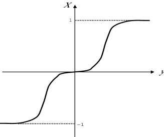
Figure 1: Schematic picture of $X$ as a function of $y$.

$$\begin{array}[]{cc}\epsfbox{A1.eps}\hfil&\epsfbox{A2.eps}\hfil\\ \mbox{(a) Scalar field $A_{1}$. }&\quad\quad\quad\mbox{(b) Scalar field $A_{2}$. }\end{array}$$

Figure 2: Schematic pictures of the scalar fields as functions of $y$ : (a) $A_{1}$ and (b) $A_{2}$.

Lastly, let us note that the bosonic part of our model given in Eq. (12) can be promoted to a five-dimensional theory without further problems. Therefore, we can consider a five-dimensional version of our model of vector boson localization with this model. The only difference is that we can no longer make it a supersymmetric theory in five dimensions, because the theory in a system of dimension greater than or equal to five requires at least eight SUSY (${\cal N}=2$ SUSY theory). The ${\cal N}=2$ SUSY introduces more symmetry constraints that do not allow the potentials of our model.

Appendix A Solving the BPS Equation

The BPS equation in terms of the rescaled variables is given by

$$\frac{d\tilde{A}_{1}}{d\tilde{y}}=\sqrt{\tilde{A}_{1}^{2}+2\tilde{\kappa}}\left[1-\tilde{A}_{1}^{2}(\tilde{A}_{1}^{2}+2\tilde{\kappa})\right].$$ (68)

This is an integrable equation:

$$\tilde{y} = \int d\tilde{A}_{1}\frac{1}{\sqrt{\tilde{A}_{1}+2\tilde{\kappa}}[1-\tilde{A}_{1}^{2}(\tilde{A}_{1}^{2}+2\tilde{\kappa})]}$$

$$= \int d\tilde{A}_{1}\frac{1}{\sqrt{\tilde{A}_{1}+2\tilde{\kappa}}[(a-\tilde{A}_{1}^{2})(\tilde{A}_{1}^{2}+b)]}$$

$$= \int d\tilde{A}_{1}\frac{1}{\sqrt{\tilde{A}_{1}+2\tilde{\kappa}}}\left(\frac{1}{a-\tilde{A}_{1}^{2}}+\frac{1}{\tilde{A}_{1}^{2}+b}\right)\frac{1}{a+b}$$

$$= \int d\tilde{A}_{1}\frac{1}{\sqrt{\tilde{A}_{1}+2\tilde{\kappa}}}\left[(\frac{1}{\sqrt{a}-\tilde{A}_{1}}+\frac{1}{\sqrt{a}+\tilde{A}_{1}})\frac{1}{2\sqrt{2}}\right.$$

$$\left.+(\frac{1}{\tilde{A}_{1}-i\sqrt{b}}-\frac{1}{\tilde{A}_{1}+i\sqrt{b}})\frac{1}{2i\sqrt{b}}\right]\frac{1}{a+b}.$$

Then, using

$$\int\frac{d\tilde{A}}{\sqrt{\tilde{A}^{2}+2\kappa}}\frac{1}{\sqrt{a}+\tilde{A}}=\int\frac{d\tilde{A}^{\prime}}{\sqrt{(\tilde{A}^{\prime}-\sqrt{a})^{2}+2\kappa}}\frac{1}{\tilde{A}^{\prime}}$$ (70)

$$= \int\frac{d\tilde{A}^{\prime}}{\tilde{A}^{\prime}}\frac{1}{\sqrt{\tilde{A}^{\prime}{}^{2}-2\sqrt{a}\tilde{A}^{\prime}+a+2\kappa}}$$

$$= \frac{1}{\sqrt{a+2\kappa}}{\rm ln}\left[\frac{\tilde{A}^{\prime}}{-2\sqrt{a}\tilde{A}^{\prime}+2(a+2\kappa)+2\sqrt{(a+2\kappa)(\tilde{A}^{\prime}{}^{2}-2\sqrt{a}\tilde{A}^{\prime}+a+2\kappa)}}\right]$$

$$= \frac{1}{\sqrt{a+2\kappa}}{\rm ln}\left[\frac{\tilde{A}+\sqrt{a}}{-2\sqrt{a}(\tilde{A}+\sqrt{a})+2(a+2\kappa)+2\sqrt{(a+2\kappa)(\tilde{A}^{2}+2\kappa)}}\right]$$

$$= \frac{1}{\sqrt{a+2\kappa}}{\rm ln}\left[\frac{\tilde{A}+\sqrt{a}}{-2\sqrt{a}\tilde{A}+4\kappa+2\sqrt{(a+2\kappa)(\tilde{A}^{2}+2\kappa)}}\right]$$

and

$$\int\frac{d\tilde{A}}{\sqrt{\tilde{A}^{2}+2\kappa}}\frac{1}{\sqrt{a}-\tilde{A}}=-\frac{1}{\sqrt{a+2\kappa}}{\rm ln}\left[\frac{-\tilde{A}+\sqrt{a}}{2\sqrt{a}\tilde{A}+4\kappa+2\sqrt{(a+2\kappa)(\tilde{A}^{2}+2\kappa)}}\right],$$ (71)

we have

$$\int\frac{d\tilde{A}}{\sqrt{\tilde{A}^{2}+2\kappa}}\left(\frac{1}{\sqrt{a}+\tilde{A}}+\frac{1}{\sqrt{a}-\tilde{A}}\right)\frac{1}{2\sqrt{a}}$$

$$=\frac{1}{2\sqrt{a(a+2\kappa)}}{\rm ln}\left(\frac{(\tilde{A}+\sqrt{a})[\sqrt{a}\tilde{A}+2\kappa+\sqrt{(a+2\kappa)(\tilde{A}^{2}+2\kappa)}]}{(\sqrt{a}-\tilde{A})[-\sqrt{a}\tilde{A}+2\kappa+\sqrt{(a+2\kappa)(\tilde{A}^{2}+2\kappa)}]}\right).$$ (72)

Thus, we obtain the result (21).

To obtain the asymptotic behavior of the BPS solution (21), we take the limit $y\to\infty$, finding $\tilde{A}\to\sqrt{a}$ and

$$\tilde{y}-\tilde{y}_{0} \sim \frac{1}{2(a+b)\sqrt{a(a+2\tilde{\kappa})}}{\rm ln}\left(\frac{2\sqrt{a}(a+2\tilde{\kappa}+a+2\tilde{\kappa})}{(\sqrt{a}-\tilde{A})(a+2\tilde{\kappa}-a+2\tilde{\kappa})}\right)+{\rm const}$$ (73)

$$\sim -\frac{1}{2(a+b)\sqrt{a(a+2\tilde{\kappa})}}{\rm ln}(\sqrt{a}-\tilde{A})+{\rm const}$$

$$\to \sqrt{a}-\tilde{A}\sim e^{-2(a+b)\sqrt{a(a+2\tilde{\kappa})}(\tilde{y}-\tilde{y}_{0})}.$$

Also, for $y\to-\infty$, we obtain $\tilde{A}\to-\sqrt{a}$ and

$$\tilde{y}-\tilde{y}_{0} \sim \frac{1}{2(a+b)\sqrt{a(a+2\tilde{\kappa})}}{\rm ln}\left(\frac{(\tilde{A}+\sqrt{a})(a+2\tilde{\kappa}-a+2\tilde{\kappa})}{2\sqrt{a}(a+2\tilde{\kappa}+a+2\tilde{\kappa})}\right)+{\rm const}$$ (74)

$$\sim \frac{1}{2(a+b)\sqrt{a(a+2\tilde{\kappa})}}{\rm ln}(\sqrt{a}+\tilde{A})+{\rm const}$$

$$\to \sqrt{a}+\tilde{A}\sim e^{+2(a+b)\sqrt{a(a+2\tilde{\kappa})}(\tilde{y}-\tilde{y}_{0})}.$$

Appendix B Mode Equation of the Vector Field

To analyze the spectra of fields $v_{m}$, let us first show that there are no zero modes. If there is a zero mode, (28) and (30) become

$$0 = v_{\nu}^{\prime\prime}-\partial_{\nu}\partial^{\mu}v_{\mu}-\partial_{\nu}v_{y}^{\prime}-V(y)v_{\nu},$$ (75)

$$0 = -\partial^{\mu}v_{\mu}^{\prime}-V(y)v_{y},$$ (76)

because a zero mode is defined by $\square v_{m}=0$. Then, applying $\partial^{\nu}$ to (75), we obtain

$$0 = (\partial_{y}^{2}-V(y))\partial^{\nu}v_{\nu}.$$ (77)

The positive definite potential $V(y)$ allows no normalizable solution, that is no solution satisfying $\partial^{\nu}v_{\nu}=0$. Then, inserting this result into (76), we obtain immediately

$$v_{y} = 0.$$ (78)

Then, inserting these results into (75), we obtain $0=(\partial_{y}^{2}-V(y))v_{\nu},$ implying

$$v_{\nu}=0.$$ (79)

Therefore we find that there is no zero mode.

Next, we decompose the linearized equations of motion into transverse and longitudinal components. Since there is no zero mode, we can separate the transverse component $\tilde{v}_{\mu}$ from the longitudinal one $\partial^{\lambda}v_{\lambda}$, as in Eq. (31). Equation (28) can be rewritten in terms of the transverse and longitudinal components as

$$0 = \square\tilde{v}_{\nu}+\tilde{v}_{\nu}^{\prime\prime}-V(y)\tilde{v}_{\nu}+\partial_{\nu}\left[{1\over\square}\left(\partial_{y}^{2}-V(y)\right)\partial^{\lambda}v_{\lambda}-v_{y}^{\prime}\right].$$ (80)

By applying $\partial^{\nu}$ to this, we can eliminate the transverse component and obtain

$$0 = \left(\partial_{y}^{2}-V(y)\right)\partial^{\lambda}v_{\lambda}-\square v_{y}^{\prime}.$$ (81)

Inserting this result into (80), we obtain the linearized equations of motion for the transverse component, as given in Eq. (33). Thus we find that the linearized equations of motion for the transverse component are decoupled from the longitudinal component $\partial^{\lambda}v_{\lambda}$ and the $y$ component $v_{y}$.

The linearized equations of motion for the longitudinal component can also be obtained. By applying $\partial_{y}$ to Eq. (30), we obtain

$$0 = \square v_{y}^{\prime}-\partial^{\lambda}v_{\lambda}^{\prime\prime}-\left(V(y)v_{y}\right)^{\prime}.$$ (82)

Then, adding this to (81), we obtain the longitudinal component in terms of $v_{y}$:

$$\partial^{\lambda}v_{\lambda} = -{1\over V(y)}\left(V(y)v_{y}\right)^{\prime}.$$ (83)

Inserting this relation into Eq. (30), we finally obtain the linearized equations of motion for $v_{y}$:

$$0 = \square v_{y}+\left({1\over V}(Vv_{y})^{\prime}\right)^{\prime}-V(y)v_{y}.$$ (84)

Appendix C Variational Approach for the Ground State

Employing the ground state wave function for the rigid wall potential (43) with width $2a/\mu$, we obtain the expectation value of the Hamiltonian in Eq. (35) to be

$$\langle H\rangle(a)=\mu^{2}\left[\left({\pi\over 2a}\right)^{2}+{\alpha^{2}\over\pi}{1\over{2a\over\alpha\pi}+{\alpha\pi\over 2a}}{\rm sinh}{2a\over\alpha}\right].$$ (85)

The minimum of this expectation value is realized at stationary point with respect to $a$, which is accurately approximated by

$$0={1\over\mu^{2}}{d\langle H\rangle\over da}\approx-\left({\pi\over 2}\right)^{2}{2\over a^{3}}+{\alpha^{2}\over 2a}{\rm e}^{2a\over\alpha}$$ (86)

for large values of $a/\alpha$, because we are interested in the case described by Eq. (39). This transcendental equation can be solved iteratively as

$${a\over\alpha}={\rm log}\left({\pi\over\alpha^{2}}\right)-{\rm log}\left({a\over\alpha}\right)\approx{\rm log}\left({\pi\over\alpha^{2}}\right)-{\rm log}{\rm log}\left({\pi\over\alpha^{2}}\right)+\cdots,$$ (87)

determining the width $a$ as given in Eq. (45). We see that this result confirms the validity of our approximation for large $a/\alpha$. At the minimum of $\langle H\rangle$ with respect to the variational parameter $a$ for small $\alpha$, we find that the kinetic energy is dominant, and that the upper bound for the ground state mass squared is given by (44).

References

• [1] N. Arkani-Hamed, S. Dimopoulos and G. Dvali, Phys. Lett. B429 (1998), 263; hep-ph/9803315. I. Antoniadis, N. Arkani-Hamed, S. Dimopoulos and G. Dvali, Phys. Lett. B436 (1998), 257; hep-ph/9804398.
• [2] L. Randall and R. Sundrum, Phys. Rev. Lett. 83 (1999), 3370; hep-ph/9905221. L. Randall and R. Sundrum, Phys. Rev. Lett. 83 (1999), 4690; hep-th/9906064.
• [3] P. Horava, and E. Witten, Nucl.Phys. B475 (1996), 94; hep-th/9603142.
• [4] V. A. Rubakov, Phys. Usp. 44 (2001), 871; hep-ph/0104152.
• [5] R. Jackiw and C. Rebbi, Phys. Rev. D13 (1976), 3398.
• [6] V. A. Rubakov and M. E. Shaposhnikov, Phys. Lett. B125 (1983), 136.
• [7] K. Akama, Lect. Notes Phys. 176 (1982), 267; hep-th/0001113.
• [8] S. L. Dubovsky and V. A. Rubakov, Int. J. Mod. Phys. A16 (2001), 4331; hep-th/0105243.
• [9] G. R. Dvali and M. A. Shifman, Phys. Lett. B396 (1997), 64 [Erratum  B407 (1997), 452]; hep-th/9612128.
• [10] T. Gherghetta and M. E. Shaposhnikov, Phys. Rev. Lett. 85 (2000), 240; hep-th/0004014.
• [11] I. Oda, Phys. Lett. B496 (2000), 113; hep-th/0006203.
• [12] S. L. Dubovsky, V. A. Rubakov and P. G. Tinyakov, J.High Energy Phys. 0008 (2000), 041; hep-ph/0007179.
• [13] M. Giovannini, H. Meyer and M. E. Shaposhnikov, Nucl. Phys. B619 (2001), 615; hep-th/0104118.
• [14] A. Neronov, Phys. Rev. D64 (2001), 044018; hep-th/0102210.
• [15] M. Giovannini, Phys. Rev. D66 (2002), 044016; hep-th/0205139.
• [16] M. Giovannini, J. V. Le Be and S. Riederer, Class. Quant. Grav. 19 (2002), 3357; hep-th/0205222.
• [17] A. Pomarol, Phys. Lett. B486 (2000), 153; hep-ph/9911294.
• [18] A. Kehagias and K. Tamvakis, Phys. Lett. B504 (2001), 38; hep-th/0010112.
• [19] I. Oda, hep-th/0103052.
• [20] I. Oda, hep-th/0103257.
• [21] K. Ghoroku, M. Tachibana and N. Uekusa, Phys. Rev. D68 (2003), 125002; hep-th/0304051.
• [22] S. Dimopoulos and H. Georgi, Nucl. Phys.  B193 (1981), 150; N. Sakai, Z. Phys. C11 (1981), 153; E. Witten, Nucl. Phys.  B188 (1981), 513; S. Dimopoulos, S. Raby, and F. Wilczek, Phys. Rev.  D24 (1981), 1681.
• [23] E. Bogomol’nyi, Sov. J. Nucl. Phys.  24 (1976), 449; M. K. Prasad and C. H. Sommerfield, Phys. Rev. Lett.  35 (1975), 760.
• [24] E. Witten and D. Olive, Phys. Lett.  B78 (1978), 97.
• [25] M. Shifman, and A. Yung, Phys. Rev. D67 (2003), 125007; hep-th/0212293.
• [26] J. Wess and J. Bagger, Supersymmetry and Supergravity, (Princeton University Press, 1991).
• [27] M. Cvetic, F. Quevedo, and S. Rey, Phys. Rev. Lett. 67 (1991), 1836; M. Cvetic, S. Griffies and S. Rey, Nucl. Phys.  B381 (1992), 301; hep-th/9201007. G. Dvali and M. Shifman, Phys. Lett.  B396 (1997), 64; hep-th/9612128. B. Chibisov and M. Shifman, Phys. Rev.  D56 (1997), 7990; hep-th/9706141.
• [28] H. Oda, K. Ito, M. Naganuma and N. Sakai, Phys. Lett.  B471 (1999), 148; hep-th/9910095.
• [29] Y. Isozumi, K. Ohashi, and N. Sakai, J. High Energy Phys. 11 (2003), 061; hep-th/0310130. J. High Energy Phys. 11 (2003), 060; hep-th/0310189.