INLO-PUB-06/03

Constituent monopoles through the eyes of fermion zero-modes
Falk Bruckmann, Dániel Nógrádi and Pierre van Baal
Instituut-Lorentz for Theoretical Physics, University of Leiden,
P.O.Box 9506, NL-2300 RA Leiden, The Netherlands

Abstract

We use the fermion zero-modes in the background of multi-caloron solutions with non-trivial holonomy as a probe for constituent monopoles. We find in general indication for an extended structure. However, for well separated constituents these become point-like. We analyse this in detail for the $SU(2)$ charge 2 case, where one is able to solve the relevant Nahm equation exactly, beyond the piecewize constant solutions studied previously. Remarkably the zero-mode density can be expressed in the high temperature limit as a function of the conserved quantities that classify the solutions of the Nahm equation.

1 Introduction

To describe regular monopoles in gauge theories a Higgs field is required. This defines the abelian subgroup of the gauge field. Yet in the full non-abelian theory there is no Dirac string and a regular solution results, the well-known ’t Hooft-Polyakov monopole [1]. In the strong interactions no such Higgs field should be present, but nevertheless it has been conjectured that a dual superconductor description, in which monopoles form the dual charges that condense, could explain confinement [2]. This scenario receives some support from the studies in supersymmetric theories through Seiberg-Witten duality [3], although also the old center vortex picture is still under active study [4]. Lattice studies based on abelian and center projections, and their respective notions of dominance [5] are the main means through which one tries to address these issues. One relies on so-called gauge fixing singularities to identify the relevant monopole [6] or center vortex degrees of freedom.

A more recent alternative to study the monopole content of gauge theories, without the need of addressing singular configurations, gauge fixing, nor introducing an extra Higgs field, has been through calorons, which are instantons at finite temperature. It has been found that calorons are actually made up from constituent monopoles [7, 8, 9], which becomes most apparent when the background Polyakov loop is non-trivial (as in the confined phase), and the size of the caloron is larger than the inverse temperature (the extent of the euclidean time direction). The background Polyakov loop is defined in the periodic gauge $A_{\mu}(\vec{x},t)=A_{\mu}(\vec{x},t+\beta)$ by its asymptotic value, or the so-called holonomy,

$${{\cal P}_{\infty}}=\lim_{x\to\infty}{\rm Pexp}(\int_{0}^{\beta}A_{0}(\vec{x},t)dt)=g^{\dagger}\exp(2\pi i{\rm diag}(\mu_{1},\mu_{2},\ldots,\mu_{n}))g,$$ (1)

where $g$ is the gauge rotation used to diagonalize ${{\cal P}_{\infty}}$, whose eigenvalues $\exp(2\pi i\mu_{j})$ can be ordered on the circle such that $\mu_{1}\leq\mu_{2}\leq\ldots\leq\mu_{n}\leq\mu_{n+1}$, with $\mu_{n+j}\equiv 1+\mu_{j}$ and $\sum_{i=1}^{n}\mu_{i}=0$. The masses of the constituent monopoles are given by $8\pi^{2}\nu_{j}/\beta$, with $\nu_{j}\equiv\mu_{j+1}-\mu_{j}$, which add up to $8\pi^{2}/\beta$, consistent with the instanton action.

Solutions are known explicitly [10] for $SU(n)$ charge 1 calorons. The $n$ constituents can have any spatial location, although all have the same location in time (they do, however, become static when well separated), and $n-1$ abelian phases complete its $4n$ parameters. Charge $k$ calorons can be viewed as composed of $kn$ monopoles, of which a class of axially symmetric configurations was constructed explicitly [11].

The purpose of this paper is to study in more detail these higher charge calorons, where the emphasis is on constructing the chiral fermion zero-modes. Charge 1 calorons have exactly one fermion zero-mode, which was shown for well separated constituents to be supported on one and only one constituent [12, 13]. We may change the constituent that supports the zero-mode, by changing the fermion boundary conditions from (anti)periodic, to being periodic up to a phase $\exp(2\pi iz)$ (from now on we will use the classical scale invariance to set $\beta=1$). For $z\in[\mu_{j},\mu_{j+1}]$ the zero-mode is localized to what we will call type $j$ constituent monopoles (with mass $8\pi^{2}\nu_{j}$, and the appropriate $U^{n-1}(1)$ charge associated to their embedding in $SU(n)$).

Lattice evidence has been gathered over recent years that these monopole constituents are present in dynamical configurations in the confined phase of gauge theories for $SU(2)$ using cooling [14, 15], and for $SU(3)$ using fermion zero-modes [16] as a filter. It is somewhat of a puzzle that these constituent monopoles had not been seen in earlier cooling studies (apart from when using twisted boundary conditions [17]). That they remained unnoticed when using fermion zero-modes as a filter is, however, simply a consequence of the fact that these studies were restricted to the use of fixed fermion boundary conditions. Only when cycling through boundary conditions specified by periodicity up to a phase, the $SU(3)$ charge 1 instanton configurations will show three separate constituent monopoles. In Fig. 2 we show a typical example based on the exact solutions for $SU(3)$, closely following the observed behavior [16] based on actual lattice simulations in the confined phase, which guarantees the background Polyakov loop to be non-trivial. In the high temperature phase, where the Polyakov loop is trivial, two of the constituents are massless and only one peak will be seen. These massless constituents are interesting in their own right, giving rise to so-called non-abelian clouds [18], but they will not concern us here.

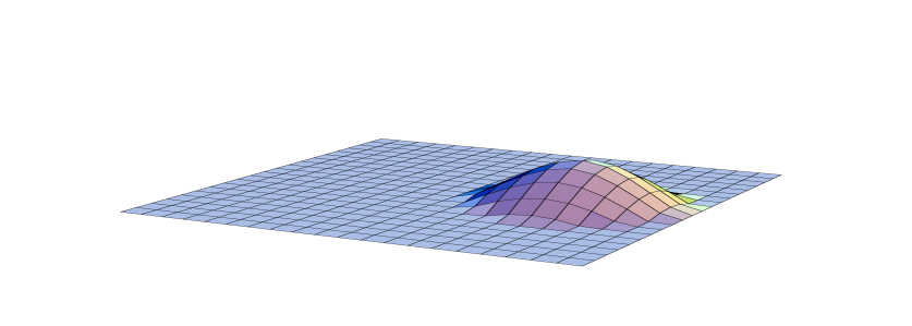
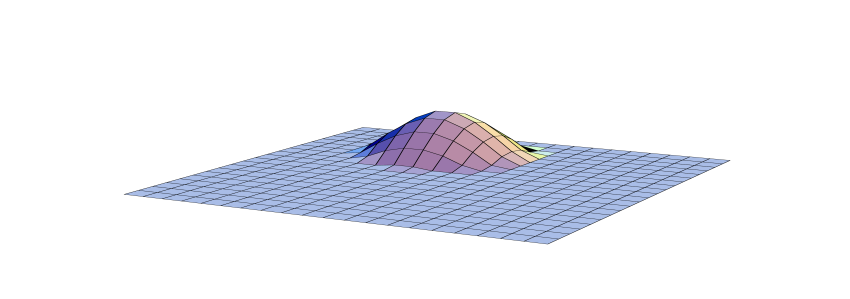
$z=12/60$                           $z=19/60$                           $z=30/60$
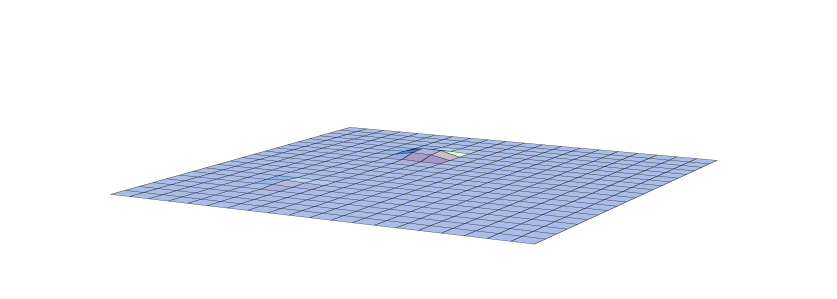
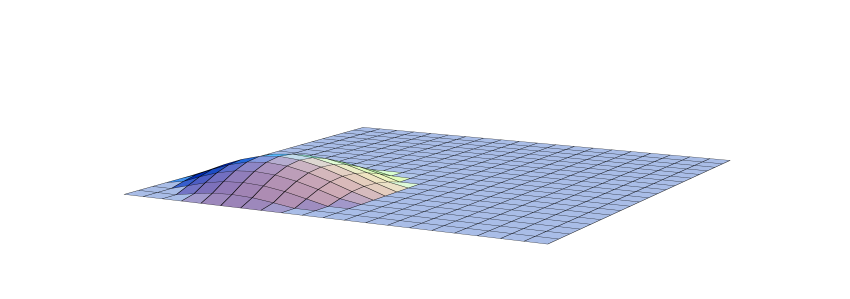
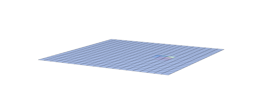
     $z=43/60$                           $z=48/60$                           $z=58/60$
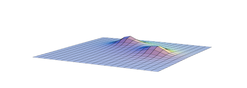
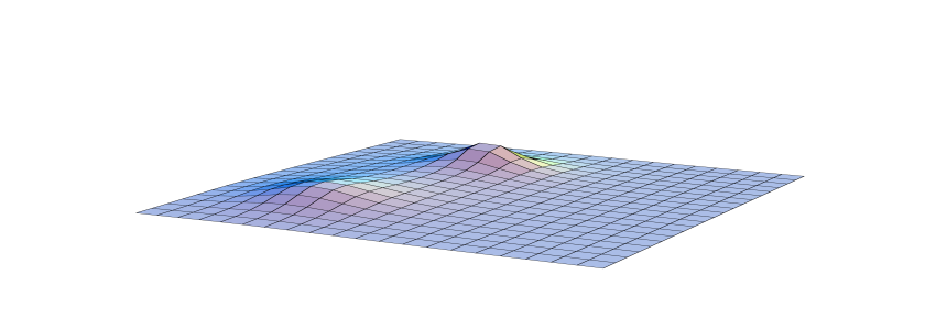
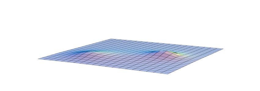
   $z=19/60$                           $z=43/60$                           $z=58/60$

Figure 1: The logarithm of the properly normalized zero-mode density for a typical $SU(3)$ caloron of charge 1, cycling through $z$. Shown are $z=\mu_{j}$ (for linear plots see Fig. 2) and three values of $z$ roughly in the middle of each interval $z\in[\mu_{j},\mu_{j+1}]$. All plots are on the same scale, cutoff for values of the logarithm below -5. The zero-mode with anti-periodic boundary conditions is found at $z=30/60$. For the action density of the associated gauge field, see Ref. [13, 19].

Figure 2: The properly normalized delocalized zero-mode densities for $z=\mu_{j}$, on a linear scale (cmp. Fig. 2).

We do not only study the fermion zero-modes for the higher charge calorons to compare with lattice simulations, but also as a tool to understand to which extend the constituent monopoles can be unambiguously identified in the caloron solutions. In the high temperature limit the non-abelian cores of the monopoles shrink to zero-sizes, and one is left with abelian gauge fields. Without taking the high temperature limit, but excluding the non-abelian cores, the same physics describes what we called the far field region [11]. It would be desirable if the abelian field in this region is described by point-like Dirac monopoles (actually dyons because of self-duality), when the constituents are well separated. For charge 1 calorons and the class of axially symmetric solutions studied before [11] the density of the fermion zero-modes become Dirac delta functions at the locations of the constituent monopoles in the high temperature limit, for any constituent separation. This infinite localization in the high temperature limit can be understood from the fact that for most $z$ values there is an effective mass for the fermions. Therefore, by studying these zero-modes in the general case, we hope to learn more about the localization of the monopoles.

It is not directly obvious that any higher charge caloron can be described by point-like constituents in the far field limit. The tool to construct these solutions is the Nahm equation [20, 7], which is a duality transformation that maps the problem of finding charge $k$ calorons to that of $U(k)$ gauge fields on a circle with specific singularities at $z=\mu_{j}$. In the cases studied so far, the dual (Nahm) gauge field can be made piecewize constant, from which one easily reads off the constituent monopole locations. In general, however, the Nahm gauge fields depend non-trivially on $z$, and it is important to understand what this implies for the localization of the constituents. Quite remarkably, we will nevertheless find that in the high temperature limit the fermion zero-mode density does not depend on $z$ and can be expressed in terms of the conserved quantities of the Nahm equation. We compute it explicitly for charge 2, revealing in general an extended structure. However, the extended structure collapses to isolated points for well separated constituents. This is so as long as $z\neq\mu_{j}$, which is the value where the localization of the zero-modes jumps. We separately study in the high temperature limit the case where $z=\mu_{j}$, for which the fermion zero-modes delocalize (decaying algebraically). Support of the zero-modes is now on constituent monopoles of types $j-1$ and $j$. We analyse this in detail for the class of axially symmetric solutions of Ref. [11], in the light of some puzzles concerning so-called bipole zero-modes [21].

This paper is organized as follows: first we describe the caloron zero-modes in Sect. 2 and set up the Green’s function calculation in Sect. 3, to be able to discuss the zero-mode and far field limits. Sect. 4 deals with the case where $z=\mu_{j}$, for which zero-modes are delocalized. In Sect. 5 we relate the zero-mode density for $z\neq\mu_{j}$ to conserved quantities of the Nahm equation and study in Sect. 6 the general solution for $SU(2)$ charge 2 caloron. We conclude with a discussion of the implications of our results and the problems that still need to be addressed. Two appendices provide the details for the zero-mode and far field limit calculations.

2 Fermion zero-modes

We wish to construct the zero-modes of the chiral Dirac equation in the background of a self-dual gauge field at finite temperature. The Dirac equation in its two-component Weyl form, with $\bar{\sigma}_{\mu}=\sigma_{\mu}^{\dagger}=({\Eins}_{2},-i\vec{\tau})$ ($\tau_{i}$ are the usual Pauli matrices), reads

$$\bar{D}\hat{\Psi}_{z}(x)\equiv\bar{\sigma}_{\mu}D_{\mu}\hat{\Psi}_{z}(x)\equiv\bar{\sigma}_{\mu}(\partial_{\mu}+A_{\mu}(x))\hat{\Psi}_{z}(x).$$ (2)

Assuming the gauge field is periodic in the imaginary time direction, with period $\beta=1$, we seek the zero-modes that satisfy the boundary condition

$$\hat{\Psi}_{z}(t+1,\vec{x})=\exp(-2\pi iz)\hat{\Psi}_{z}(t,\vec{x}),$$ (3)

A simple abelian gauge transformation, $\Psi_{z}(x)=\exp(2\pi izt)\hat{\Psi}_{z}(x)$, makes the zero-mode periodic. This gauge transformation replaces the gauge field by $A_{\mu}(x)-2\pi iz_{\mu}{\Eins}_{n}$, but it does not change the field strength, such that existence of the appropriate number of zero-modes is guaranteed by the index theorem.

The caloron solutions are obtained by Fourier transformation, reformulating the algebraic ADHM (Atiyah-Drinfeld-Hitchin-Manin) construction [22] of multi-instanton solutions in $R^{4}$, as the Nahm transformation [7]. For this the instantons in $R^{4}$ periodically repeat themselves in the imaginary time direction up to a gauge rotation with ${{\cal P}_{\infty}}$. This Fourier transformation also selects out of the infinite number of fermion zero-modes in $R^{4}$, those that satisfy the correct periodicity.

In the ADHM formulation the $k$ normalized fermion zero-modes for a charge $k$ $SU(N)$ instanton are given by ($\varepsilon\equiv i\tau_{2}=\sigma_{2}$, $i=1,\ldots,n$ is the color index, $l=1,\ldots,k$ the charge index and $I=1,2$ the spinor index)

$$\Psi_{iI}^{l}(x)=\pi^{-1}\left(\phi^{-{\scriptstyle{{1/2}}}}(x)u^{\dagger}(x)f_{x}\varepsilon\right)_{iI}^{l},\quad\phi(x)={\Eins}_{n}+u^{\dagger}(x)u(x),$$ (4)

with $u^{\dagger}(x)$ given explicitly in terms of the ADHM parameters by

$$u^{\dagger}(x)=\lambda(B-{\Eins}_{k}x)^{-1},\quad B=\sigma_{\mu}B_{\mu},\quad x=x_{\mu}\sigma_{\mu},$$ (5)

where $\lambda=(\lambda_{1},\ldots,\lambda_{k})$, with $\lambda_{i}^{\dagger}$ a two-component spinor in the $\bar{n}$ representation of $SU(n)$ ($\lambda$ can be seen as a $n\times 2k$ complex matrix), and $B_{\mu}$ hermitian $k\times k$ matrices. As $\phi(x)$ is an $n\times n$ positive hermitian matrix (for $n=2$ proportional to ${\Eins}_{2}$), its square root is well-defined. We also recall the gauge field is given by

$$A_{\mu}(x)=\phi^{-{\scriptstyle{{1/2}}}}(x)(u^{\dagger}(x)\partial_{\mu}u(x))\phi^{-{\scriptstyle{{1/2}}}}(x)+\phi^{{\scriptstyle{{1/2}}}}(x)\partial_{\mu}\phi^{-{\scriptstyle{{1/2}}}}(x).$$ (6)

which can be shown to be self-dual provided the quadratic ADHM constraint is satisfied,

$$\lambda^{\dagger}\lambda+(B-{\Eins}_{k}x)^{\dagger}(B-{\Eins}_{k}x)=\sigma_{0}f^{-1}_{x},$$ (7)

which implicitly defines $f_{x}$ as a hermitian $k\times k$ Green’s function, thereby completing the description of Eq. (4). A further simplication [9, 23] will be helpful, which uses the fact that $2(B_{\mu}-x_{\mu})=\partial_{\mu}f_{x}^{-1}$ and $u^{\dagger}(x)=\phi(x)\lambda f_{x}(B-{\Eins}_{k}x)^{\dagger}$, implying

$$A_{\mu}(x) = {\scriptstyle{{1\over 2}}}\phi^{\scriptstyle{{1/2}}}(x)\lambda\bar{\eta}_{\mu\nu}\partial_{\nu}f_{x}\lambda^{\dagger}\phi^{\scriptstyle{{1/2}}}(x)+{\scriptstyle{{1\over 2}}}[\phi^{-{\scriptstyle{{1/2}}}}(x),\partial_{\mu}\phi^{\scriptstyle{{1/2}}}(x)],$$

$$\phi^{-1}(x) = 1-\lambda f_{x}\lambda^{\dagger},\quad\Psi_{iI}^{l}(x)=(2\pi)^{-1}(\phi^{\scriptstyle{{1/2}}}(x)\lambda\partial_{\mu}f_{x}\bar{\sigma}_{\mu}\varepsilon)_{iI}^{l},$$ (8)

with $\bar{\eta}_{\mu\nu}=\bar{\eta}^{j}_{\mu\nu}\sigma_{j}=\bar{\sigma}_{[\mu}\sigma_{\nu]}$ the anti-selfdual ’t Hooft tensor.

As mentioned above, calorons are obtained by arranging the instantons in $R^{4}$ to be periodic (up to a gauge rotation). The time interval $[0,1]$ will contain as many instantons as the topological charge of the caloron. One splits the charge index $l$ as $l=pk+a$, where $a$ labels the $k$ instantons in the interval $[0,1]$ and $p$ labels the infinite number of repeated time-intervals, playing the role of the Fourier index. We find, suppressing the gauge and spinor index (cmp. Ref. [12, 13]),

$$\hat{\Psi}_{z}^{a}(x)=(2\pi)^{-1}\phi^{\scriptstyle{{1/2}}}(x)\partial_{\mu}\int_{0}^{1}dz^{\prime}\hat{\lambda}_{b}(z^{\prime})\hat{f}^{ba}_{x}(z^{\prime},z)\bar{\sigma}_{\mu}\varepsilon.$$ (9)

where the Fourier transforms of $\lambda$ and $f_{x}$ are denoted by $\hat{\lambda}_{a}(z)$ and $\hat{f}_{x}^{ba}(z^{\prime},z)$. The fermion zero-modes thus constructed are in the so-called algebraic gauge, for which $\hat{\Psi}_{z}(t+1,\vec{x})=\exp(-2\pi iz){{\cal P}_{\infty}}\hat{\Psi}_{z}(t,\vec{x})$. In this gauge all components of $A_{\mu}$ vanish at spatial infinity and the non-trivial holonomy is encoded in the boundary condition, which for the gauge field reads $A_{\mu}(t+1,\vec{x})={{\cal P}_{\infty}}A_{\mu}(t,\vec{x}){\cal P}_{\infty}^{-1}$. A simple time-dependent gauge transformation allows one to transform to the periodic gauge, after which $A_{0}$ goes to a constant at spatial infinity.

To encode the appropriate periodicity in the ADHM parameters we need to take $\lambda_{pk+a}={\cal P}_{\infty}^{p}\zeta_{a}$ [11]. Introducing the projections $P_{m}$ on the eigenvalues of ${{\cal P}_{\infty}}$, i.e. ${{\cal P}_{\infty}}\equiv\sum_{m=1}^{n}\exp(2\pi i\mu_{m})P_{m}$, we find $\hat{\lambda}_{a}(z)=\sum_{m=1}^{n}\delta(z-\mu_{m})P_{m}\zeta_{a}$, which makes the expression for the zero-modes particularly simple,

$$\hat{\Psi}_{z}^{a}(x)=(2\pi)^{-1}\phi^{\scriptstyle{{1/2}}}(x)\sum_{m=1}^{n}P_{m}\zeta_{b}\bar{\sigma}_{\mu}\varepsilon\partial_{\mu}\hat{f}^{ba}_{x}(\mu_{m},z).$$ (10)

The fact that we are dealing with higher charge calorons, is reflected in the presence of the indices $a,b=1,\ldots,k$. Making use of the well-known identity [23, 24, 25] in $R^{4}$, $\Psi_{iI}^{l}(x)^{*}\Psi_{iI}^{m}(x)=-(2\pi)^{-2}\partial_{\mu}^{2}f^{lm}_{x}$, Fourier transformation gives the appropriate expression for the caloron zero-mode density

$$\hat{\Psi}_{z}^{a}(x)^{\dagger}\hat{\Psi}_{z}^{b}(x)=-(2\pi)^{-2}\partial_{\mu}^{2}\hat{f}^{ab}_{x}(z,z).$$ (11)

Using the fact that $\lim_{|\vec{x}|\rightarrow\infty}|\vec{x}|\hat{f}^{ab}_{x}(z,z)=\pi\delta^{ab}$, the zero-modes $\hat{\Psi}_{z}^{a}$ are seen to be orthonormal.

We close this section by remarking that for $SU(2)$ an alternative construction is possible, as part of the $Sp(n)$ series (since $Sp(1)=SU(2)$). The ADHM construction for $Sp(n)$ is based on quaternions. In particular $\lambda_{l}$ is assumed to be a quaternion, whereas $B_{\mu}$ is now real-symmetric. All formulae presented above remain valid, but it should be noted that the transformation $\lambda\rightarrow\lambda T^{\dagger}$, $B_{\mu}\rightarrow TB_{\mu}T^{\dagger}$, with $T\in U(k)$, leaving the gauge field and the ADHM constraint untouched, has to be replaced by $T\in O(k)$.

3 Zero-mode and far field limit

As we have seen above, all physical quantities can be reconstructed, once we have found the Green’s function $\hat{f}^{ab}_{x}(z,z^{\prime})$. Here we review the necessary ingredients. We start with the fact that the Green’s function is defined through an impurity scattering problem [11]

$$\left\{-\frac{d^{2}}{dz^{2}}+V(z;\vec{x})\right\}\!f_{x}(z,z^{\prime})=4\pi^{2}{\Eins}_{k}\delta(z\!-\!z^{\prime}),$$ (12)

where $f_{x}(z,z^{\prime})$ is related to $\hat{f}_{x}(z,z^{\prime})$ by a $U(k)$ gauge transformation

$$f_{x}(z,z^{\prime})=\hat{g}(z)\hat{f}_{x}(z,z^{\prime})\hat{g}^{\dagger}(z^{\prime}),\quad\hat{g}(z)=\exp\left(2\pi i(\xi_{0}-x_{0}{\Eins}_{k})z\right).$$ (13)

The “potential” $V$, which includes “impurity” contributions, is determined by the (dual) $U(k)$ Nahm gauge field $\hat{A}_{\mu}(z)$

$$V(z;\vec{x})=4\pi^{2}\vec{R}^{2}(z;\vec{x})+2\pi\sum_{m}\delta(z-\mu_{m})S_{m},\quad S_{m}=\hat{g}(\mu_{m})\hat{S}_{m}\hat{g}^{\dagger}(\mu_{m}),$$

$$R_{j}(z;\vec{x})=x_{j}{\Eins}_{k}-(2\pi i)^{-1}\hat{g}(z)\hat{A}_{j}(z)\hat{g}^{\dagger}(z),\qquad\,\hat{S}_{m}^{ab}=\pi{\rm tr}_{2}(\zeta_{a}^{\dagger}P_{m}\zeta_{b}).$$ (14)

Fourier transformation of $B_{\mu}$ gives $(2\pi i)^{-1}\delta(z-z^{\prime})(\delta_{\mu 0}{\Eins}_{k}{\frac{d}{dz}}+\hat{A}_{\mu}(z))$ and defines the Nahm gauge field. We have further used the fact that one can choose a $U(k)$ gauge in which $\hat{A}_{0}(z)\equiv 2\pi i\xi_{0}$ is constant, which itself can be transformed to zero by $\hat{g}(z)$. Note that $\hat{g}(1)$ plays the role of the holonomy associated to the dual Nahm gauge field $\hat{A}_{\mu}(z)$. Crucial is that we can formulate the zero-mode and far field limits without specifying the solutions of the Nahm equations. These Nahm equations, which are equivalent to the ADHM constraint, are given by

$${\frac{d}{dz}}\hat{A}_{j}(z)+[\hat{A}_{0}(z),\hat{A}_{j}(z)]+{\scriptstyle{{1\over 2}}}\varepsilon_{jk\ell}[\hat{A}_{k}(z),\hat{A}_{\ell}(z)]=2\pi i\sum_{m}\delta(z-\mu_{m})\rho_{m}^{\,j},$$

$$\hskip 113.81102pt\vec{\rho}_{m}^{\,ab}\equiv-\pi{\rm tr}_{2}\left(\zeta_{a}^{\dagger}P_{m}\zeta_{b}\vec{\tau}\right).$$ (15)

This will be discussed in more detail in Sect. 6.

To solve the second order equation for $f_{x}(z,z^{\prime})$ it is convenient to convert it to a first order equation, involving $2k\times 2k$ matrices,

$$\left({\frac{d}{dz}}-\pmatrix{0&{\Eins}_{k}\cr V(z;\vec{x})&0\cr}\right)\pmatrix{\quad f_{x}(z,z^{\prime})\cr{\frac{d}{dz}}f_{x}(z,z^{\prime})\cr}=-4\pi^{2}\delta(z-z^{\prime})\pmatrix{0\cr{\Eins}_{k}\cr},$$ (16)

which can be solved as

$$\pmatrix{\quad f_{x}(z,z^{\prime})\cr{\frac{d}{dz}}f_{x}(z,z^{\prime})\cr}=-4\pi^{2}W(z,z_{0})\left\{({\Eins}_{2k}-{\cal{F}}_{z_{0}})^{-1}-\theta(z^{\prime}-z){\Eins}_{2k}\right\}W^{-1}(z^{\prime},z_{0})\pmatrix{0\cr{\Eins}_{k}\cr},$$ (17)

where $z_{0}$ can be arbitrary and

$$W(z_{2},z_{1})={\rm Pexp}\left[\int_{z_{1}}^{z_{2}}\pmatrix{0&{\Eins}_{k}\cr V(z;\vec{x})&0\cr}dz\right],\quad{\cal{F}}_{z_{0}}=\hat{g}^{\dagger}(1)W(z_{0}+1,z_{0}).$$ (18)

In particular, one can show that [11]

$$-{\scriptstyle{{1\over 2}}}{\rm Tr}_{n}F_{\mu\nu}^{2}(x)=-{\scriptstyle{{1\over 2}}}\partial_{\mu}^{2}\partial_{\nu}^{2}\log\psi(x),\quad\psi=\det\left(ie^{-\pi ix_{0}}({\Eins}_{2k}-{\cal{F}}_{z_{0}})/\sqrt{2}\right).$$ (19)

To isolate the exponential contributions in Eq. (18), one introduces two solutions of the Riccati equation [11],

$$R_{m}^{\pm}(z)^{2}\pm\frac{1}{2\pi}\frac{d}{dz}\,R_{m}^{\pm}(z)=\vec{R}^{2}(z;\vec{x}).$$ (20)

Since $\vec{R}(z;\vec{x})\to\vec{x}{\Eins}_{k}$ for $|\vec{x}|\to\infty$, we find in this limit that $R_{m}^{\pm}(z)\to|\vec{x}|{\Eins}_{k}$. Defining

$$f_{m}^{\pm}(z)=P\exp\left[\pm 2\pi\int_{\mu_{m}}^{z}\!\!\!R_{m}^{\pm}(z)dz\right],\quad z\in[\mu_{m},\mu_{m+1}],$$ (21)

we see that $f_{m}^{\pm}(z)\to\exp\left(\pm 2\pi|\vec{x}|(z-\mu_{m}){\Eins}_{k}\right)$. These are the exponentially rising and decaying solutions of Eq. (12), in terms of which we can rewrite for $z,z^{\prime}\in(\mu_{m},\mu_{m+1})$

$$W(z,z^{\prime})=W_{m}(z)W_{m}^{-1}(z^{\prime}),\quad W_{m}(z)\equiv\hat{W}_{m}(z)F_{m}(z),$$ (22)

where $F_{m}(z)$ contains all exponential factors,

$$\hat{W}_{m}(z)=\pmatrix{{\Eins}_{k}&{\Eins}_{k}\cr 2\pi R^{+}_{m}(z)&-2\pi R^{-}_{m}(z)\cr},\quad F_{m}(z)=\pmatrix{f_{m}^{+}(z)&0\cr 0&f_{m}^{-}(z)\cr}.$$ (23)

As an illustration let us assume $\vec{R}(z;\vec{x})^{2}=(\vec{x}{\Eins}_{k}-\vec{e}\,Y_{m})^{2}\equiv R^{2}_{m}$, independent of $z$, for $z\in[\mu_{m},\mu_{m+1}]$, as is the case for charge one [9] and a class of axially symmetric solutions [11] (see Sect. 4). We then find $R^{+}_{m}(z)=R^{-}_{m}(z)=R_{m}$ and $f_{m}^{\pm}(z)=\exp(2\pi(z-\mu)R_{m})$. Diagonalizing $R_{m}$ defines $k$ locations (the eigenvalues of $Y_{m}$), which are sharply defined and give rise to point-like constituents in the high temperature limit. When $\vec{R}(z;\vec{x})$ is not piecewize constant, these locations are a priori not sharply defined. We still expect the cores to be the regions in $\vec{x}$ where $\vec{R}(z;\vec{x})$ remains small (cmp. Eq. (14)). The separations between the cores of monopoles of different type is controlled by the discontinuity in $\hat{A}_{j}(z)$, Eq. (15), and can in general be chosen large. This allows us to define the zero-mode limit, where $\vec{x}$ is assumed to be far removed from any constituent core not of type $m$. In technical terms that means that $R_{m^{\prime}}^{\pm}(z)$ is large for all $m^{\prime}\neq m$. Accordingly, $f_{m^{\prime}}^{-}(z)$ and $f_{m^{\prime}}^{+}(z)^{-1}$ are exponentially small for these values of $\vec{x}$ (cmp. Eq. (21)). Results that are valid up to these exponential correction are denoted by a subscript “${\rm{zm}}$” for the zero-mode limit and “${\rm{ff}}$” for the far field limit. In the latter case, $\vec{x}$ is assumed to be far removed from all constituents.

In appendix A we show that for $\mu_{m}\leq z^{\prime}\leq z\leq\mu_{m+1}$

$$f^{{\rm{zm}}}_{x}(z,z^{\prime})=\pi(e_{m}^{+}(z)-e_{m}^{-}(z)Z_{m+1}^{-})\left(e_{m}^{+}-Z_{m}^{+}e_{m}^{-}Z_{m+1}^{-}\right)^{-1}(\tilde{e}_{m}^{+}(z^{\prime})-Z_{m}^{+}\tilde{e}_{m}^{-}(z^{\prime}))R_{m}^{-1}(z^{\prime}).$$ (24)

(for $z^{\prime}>z$ one uses $f_{x}(z^{\prime},z)=f_{x}^{\dagger}(z,z^{\prime})$) with

$$e_{m}^{\pm}(z)\equiv f_{m}^{\mp}(z)f_{m}^{\mp}(\mu_{m+1})^{-1}, e_{m}^{\pm}\equiv e_{m}^{\pm}(\mu_{m}),\quad\tilde{e}_{m}^{\pm}(z)\equiv f_{m}^{\mp}(z)^{-1},$$

$$Z_{m}^{-}\equiv{\Eins}_{k}-2\Sigma_{m}^{-1}R_{m-1}(\mu_{m}), Z_{m}^{+}\equiv{\Eins}_{k}-2\Sigma_{m}^{-1}R_{m}(\mu_{m}),$$ (25)

$$R_{m}(z)\equiv{\scriptstyle{{1\over 2}}}(R_{m}^{+}(z)+R_{m}^{-}(z)), \Sigma_{m}\equiv R_{m}^{-}(\mu_{m})+R_{m-1}^{+}(\mu_{m})+S_{m}.$$

This result is valid up to exponential corrections as long as $\vec{x}$ is far removed from all constituents of type $m^{\prime}\neq m$. Note that in this limit $Z_{m}^{\pm}={\Eins}_{k}$, however, only up to algebraic corrections, which is why we have kept them. In Fig. 3 we give the zero-mode densities for a charge 2 axially symmetric solution in $SU(2)$, with well-separated constituents. We found no differences to 1 part in $10^{6}$ between the exact result and the result obtained with the zero-mode limit, Eq. (24). The choice of basis for the zero-modes involves the gauge rotation that for each interval $z\in[\mu_{m},\mu_{m+1}]$ identifies the constituent locations, cmp. Sect. 4 and Ref. [11]. This ensures that each zero-mode is localized to only one constituent monopole.

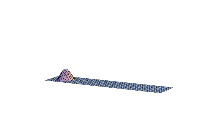
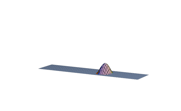
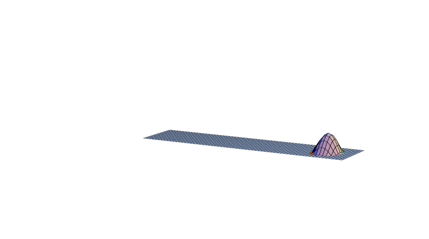
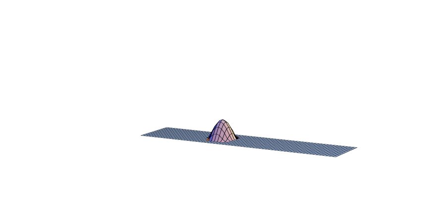
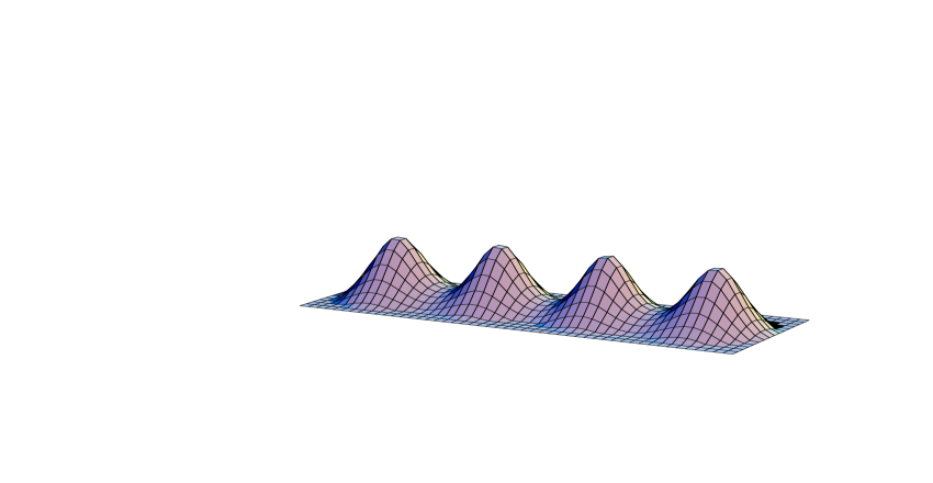
Figure 3: Zero-mode densities for a typical charge 2, $SU(2)$ axially symmetric solution. For comparison the action density (cmp. Fig. 2 of Ref. [11]) is shown in the middle. All are on a logarithmic scale, cutoff below $e^{-3}$. On the left is shown the two periodic zero-modes ($z=0$) and on the right the two anti-periodic zero-modes ($z=1/2$).

It is now almost trivial to read off from this the far field limit for $f_{x}(z,z)$, where $\vec{x}$ is assumed to be far from all constituents. As long as $z\neq\mu_{m}$ and $z\neq\mu_{m+1}$, $e_{m}^{-}(z)$ and $\tilde{e}_{m}^{-}(z)$ are exponentially small, and $f^{\rm{ff}}_{x}(z,z)=\pi e_{m}^{+}(z)(e_{m}^{+})^{-1}\tilde{e}_{m}^{+}(z)R_{m}^{-1}(z)$. But using the definitions of $e_{m}^{\pm}(z)$ and $\tilde{e}_{m}^{\pm}(z)$ all exponential factors precisely cancel and in the far field limit we are left with

$$f^{\rm{ff}}_{x}(z,z)=\pi R_{m}^{-1}(z),\quad z\in(\mu_{m},\mu_{m+1}),$$ (26)

which will play a very important role in Sects. 5 and 6. We can also read off the far field limit for $f_{x}(z,z^{\prime})$ evaluated at the impurities $\mu_{m}$ and $\mu_{m+1}$, noting that by definition $e_{m}^{\pm}(\mu_{m+1})=\tilde{e}_{m}^{\pm}(\mu_{m})={\Eins}_{k}$,

$$f^{\rm{ff}}_{x}(\mu_{m+1},\mu_{m+1}) = \pi({\Eins}_{k}-Z_{m+1}^{-})R_{m}^{-1}(\mu_{m+1})=2\pi\Sigma_{m+1}^{-1},$$

$$f^{\rm{ff}}_{x}(\mu_{m},\mu_{m}) = \pi({\Eins}_{k}-Z_{m}^{+})R_{m}^{-1}(\mu_{m})=2\pi\Sigma_{m}^{-1},$$ (27)

and $f^{\rm{ff}}_{x}(\mu_{m+1},\mu_{m})=0$ (as well as $f^{\rm{ff}}_{x}(\mu_{m},\mu_{m+1})=0$, using $f_{x}(z,z^{\prime})=f_{x}^{\dagger}(z^{\prime},z)$), verifying the results of Ref. [11]. Although $f_{x}(z,z)$ is continuous at the impurities, comparing Eq. (26) with Eq. (27) we see, as anticipated, that in the high temperature limit $f_{x}(z,z)$ is discontinuous at the impurities. At finite temperature, the transition across the impurity has a “width” inversely proportional to the temperature.

For $k=1$, where $e_{m}^{\pm}(z)=\exp(\pm 2\pi(\mu_{m+1}-z)r_{m})$ and $\tilde{e}_{m}^{\pm}(z)=\exp(\pm 2\pi(z-\mu_{m})r_{m})$ one finds for $z^{\prime},z\in(\mu_{m},\mu_{m+1})$

$$f^{\rm{zm}}_{x}(z^{\prime},z)=\frac{2\pi\sinh\left(2\pi r_{m}(\mu_{m+1}-z^{\prime}+\gamma^{-}_{m+1})\right)\sinh\left(2\pi r_{m}(z-\mu_{m}+\gamma^{+}_{m})\right)}{r_{m}\sinh\left(2\pi r_{m}(\nu_{m}+\gamma_{m}^{+}+\gamma_{m+1}^{-})\right)},$$ (28)

which agrees with the result of Ref. [13], where only the limit with $\gamma_{m}^{+}\equiv-{\scriptstyle{{1\over 2}}}\log Z_{m}^{+}$ and $\gamma_{m+1}^{-}\equiv-{\scriptstyle{{1\over 2}}}\log Z_{m+1}^{-}$ neglected and $z^{\prime}=z$ was considered. We stress again that the presence of $\gamma$ implies a subtle algebraically decaying influence due to the constituents of type $m-1$ and $m+1$ (the influence of all other constituents is decaying exponentially, although this is only relevant for $SU(n>3)$). In terms of constituent radii $r_{m}=|\vec{x}-\vec{y}_{m}|$ and locations $\vec{y}_{m}$ one has

$$Z_{m+1}^{-}=\frac{|\vec{y}_{m+1}-\vec{y}_{m}|+r_{m+1}-r_{m}}{|\vec{y}_{m+1}-\vec{y}_{m}|+r_{m+1}+r_{m}},\quad Z_{m}^{+}=\frac{|\vec{y}_{m-1}-\vec{y}_{m}|+r_{m-1}-r_{m}}{|\vec{y}_{m-1}-\vec{y}_{m}|+r_{m-1}+r_{m}}.$$ (29)

For $SU(2)$, with $\vec{y}_{m+1}=\vec{y}_{m-1}$, therefore $Z_{m}^{+}=Z_{m+1}^{-}$, or $\gamma_{m}^{+}=\gamma_{m+1}^{-}$, and the influence of the other constituent is only felt by a renormalization of the mass $\nu_{m}$,

$$SU(2):\ f^{\rm{zm}}_{x}(z,z)=\pi\frac{\cosh\left(2\pi r_{m}(\nu_{m}+2\gamma_{m})\right)-\cosh\left(2\pi r_{m}(2z-\mu_{m}-\mu_{m+1})\right)}{r_{m}\sinh\left(2\pi r_{m}(\nu_{m}+2\gamma_{m})\right)}.$$ (30)

Note that for $SU(2)$ $\mu_{1}+\mu_{2}=0$ and $\mu_{2}+\mu_{3}=1$. This leads to the well-know result for the monopole zero-mode density $f^{\rm{zm}}_{x}(z,z)=\pi r^{-1}_{m}\tanh\left(\pi r_{m}(\nu_{m}+2\gamma_{m})\right)$, with $z=0$ for $m=1$ (periodic zero-mode) and $z=1/2$ for $m=2$ (anti-periodic zero-mode).

4 Bipole zero-modes

In this section we discuss the zero-modes in the high temperature limit for $z=\mu_{m}$, which means that ${{\cal P}_{\infty}}e^{-2\pi iz}$ has one of its eigenvalues equal to 1, which leads to one of the components of the fermion to become massless. Indeed, using Eqs. (11,13,27) we find that in the far field limit

$$z=\mu_{m}:\qquad\hat{\Psi}_{z}^{a}(x)^{\dagger}\hat{\Psi}_{z}^{b}(x)=-(2\pi)^{-1}\partial_{i}^{2}\left(\hat{\Sigma}_{m}^{-1}\right)^{ab},\quad\hat{\Sigma}_{m}\equiv\hat{g}^{\dagger}(\mu_{m})\Sigma_{m}\hat{g}(\mu_{m}),$$ (31)

decays algebraically and has support on the constituents of type $m-1$ and $m$, as is easy to see for $k=1$, where $\Sigma_{m}=|\vec{x}-\vec{y}_{m-1}|+|\vec{x}-\vec{y}_{m}|+|\vec{y}_{m-1}-\vec{y}_{m}|$. Here we will restrict ourselves to $SU(2)$, particularly interesting for the axially symmetric caloron solutions, since in the high temperature limit its gauge field has the form of the so-called bipole ansatz (see Eq. (35)), which always has an integrable chiral fermion zero-mode [21]. In the bipole ansatz all Dirac strings have to run in the same direction, but other than that, the locations of the self-dual Dirac monopoles can be arbitrary. However, for the axially symmetric caloron solutions the constituents have to alternate between opposite charges on a line [11]. In this case, with the solution coming from a regular caloron, there are always as many zero-modes as the number of constituents with a given charge (equal to the topological charge $k$). By considering the case of solutions with topological charge 2, we will find the expressions for the bipole zero-mode and the extra zero-mode, in terms of the constituent locations only (which should be possible, since the abelian gauge field has this property in the high temperature limit). Remarkably, we will find that rearranging the order of the constituents, so as to violate the constraint coming from the axially symmetric caloron, the second zero-mode is no longer integrable (while the gauge field and bipole zero-mode remain well defined).

A particular class of axially symmetric caloron solutions is obtained by taking $Y^{j}_{m}\equiv\hat{g}(z)\frac{\hat{A}_{j}(z)}{2\pi i}\hat{g}^{\dagger}(z)$ to be piecewize constant. This can be shown to satisfy the Nahm or ADHM equation when we take [11]

$$\zeta_{a}=\rho_{a}\exp(2\pi i\alpha_{a})\zeta,\quad\alpha_{a}\equiv\sum_{m=1}^{n}\alpha_{a}^{m}P_{m},\quad{\rm Tr}_{n}\alpha_{a}=0,\quad\vec{Y}_{m}=Y_{m}\vec{e},$$ (32)

where $\rho_{a}$ are positive, not to be confused with

$$\vec{\rho}_{m}^{\,ab}=\rho^{a}\rho^{b}\exp(2\pi i(\alpha_{b}^{m}-\alpha_{a}^{m}))\Delta\vec{y}_{m},\quad\Delta\vec{y}_{m}=\Delta y_{m}\vec{e}\equiv-\pi{\rm tr}_{2}(\zeta^{\dagger}P_{m}\zeta\vec{\tau}).$$ (33)

For $SU(2)$ one has $\Delta\vec{y}_{1}=-\Delta\vec{y}_{2}$ (for $SU(n>2)$ a constraint on $\zeta$ is required, to guarantee that all $\Delta\vec{y}_{m}$ are parallel). We will take $\vec{e}=\Delta\vec{y}_{2}/|\Delta\vec{y}_{2}|=(0,0,1)$ (hence $\Delta y_{2}>0$) and ${{\cal P}_{\infty}}=\exp(2\pi i\mu_{2}\tau_{3})$ (therefore $\zeta=\sqrt{\Delta y_{2}/\pi}{\Eins}_{2}$). This can always be arranged to be the case by a global gauge rotation, and a spatial rotation. We define $\vec{y}_{m}$, up to an irrelevant overall shift, through $\Delta\vec{y}_{m}\equiv\vec{y}_{m}-\vec{y}_{m-1}$. This fixes $Y_{m}$ to be

$$Y_{m}^{ab}=(\xi_{a}+\rho_{a}^{2}y_{m})\delta_{ab}+i(1-\delta_{ab})\rho_{a}\rho_{b}\sum_{j=1}^{n}\Delta y_{j}\frac{\exp\left(2\pi i\left[\alpha_{b}^{j}-\alpha_{a}^{j}-(\mu_{j}+s_{j}^{m})(\xi_{0}^{b}-\xi_{0}^{a})\right]\right)}{2\sin\left(\pi\left[\xi_{0}^{b}-\xi_{0}^{a}\right]\right)}.$$ (34)

The constituent locations are found from the eigenvalues of $Y_{m}$. Although constant, it is not true in general that the $Y_{m}$ can be diagonalized simultaneously, making this a non-abelian solution of the Nahm equation. Yet, as we remarked before, one easily computes the Green’s function, since $R^{\pm}_{m}(z)=R_{m}=\sqrt{(\vec{x}{\Eins}_{k}-\vec{e}\,Y_{m})\cdot(\vec{x}{\Eins}_{k}-\vec{e}\,Y_{m})}$ is constant in $z$. Using that for the axially symmetric solutions $\vec{\rho}_{m}^{\,ab}=\hat{S}_{m}^{ab}\vec{y}_{m}/|\Delta\vec{y}_{m}|$, one shows [11] that in the high temperature limit the (abelian) gauge field can be written in the form of the bipole ansatz [21]

$$A_{\mu}(x)=-\frac{i}{2}\tau_{3}\bar{\eta}^{3}_{\mu\nu}\partial_{\nu}\log\phi(x),\quad\phi(x)=\phi_{\rm{ff}}(x)\equiv\frac{\det(R_{1}+R_{2}+S_{2})}{\det(R_{1}+R_{2}-S_{2})}.$$ (35)

In the bipole ansatz, one splits $A_{\mu}(x)$ in an isospin up and isospin down component (with inverted abelian charges). However, all that concerns us here is the fact that for any $\phi$, $A_{\mu}(x)$ as given above is self-dual (and hence a solution of the Maxwell equations) provided $\log\phi$ is harmonic away from Dirac string singularities (defined by $\phi^{-1}=0$). This always gives rise to at least one normalizable zero-mode of the chiral Dirac equation

$$\hat{\Psi}_{mI}(x)=(2\pi\tilde{\rho})^{-1}\phi^{-{\scriptstyle{{1/2}}}}(x)(\tau_{1}\bar{\sigma}_{\mu}\varepsilon)_{mI}\partial_{\mu}\log\phi(x).$$ (36)

were $\tilde{\rho}$ is simply a normalization factor. Here $m$ corresponds to the isospin component that survives for $z=\mu_{m}$ (with the other component related to $\hat{f}_{x}(\mu_{1},\mu_{2})$ vanishing in the far field limit, see Eq. (9)).

We now work out the explicit form of all $k$ zero-modes for the axially symmetric caloron solution, showing how the zero-mode in Eq. (36) is recovered from these. Using Eqs. (10,27,33), together with the fact that $\hat{f}_{x}(\mu_{1},\mu_{2})$ is exponentially small ($\tau_{1}$ is used for picking out the surviving component), we find for the normalized zero-modes at $z=\mu_{m}$ ($|\zeta|=\sqrt{\Delta y_{2}/\pi}$)

$$\hat{\Psi}_{mI}^{a}(x)=\phi_{\rm{ff}}^{{\scriptstyle{{1/2}}}}(x)|\zeta|\rho_{b}e^{2\pi i\alpha_{b}^{m}}(\tau_{1}\bar{\sigma}_{\mu}\varepsilon)_{mI}\partial_{\mu}\left(\hat{\Sigma}_{m}^{-1}\right)^{ba}.$$ (37)

Using the fact that (cmp. Eq. (8))

$$\phi^{-1}_{\rm{ff}}(x)=1-2\pi|\zeta|^{2}\rho_{a}e^{2\pi i\alpha_{a}^{m}}\left(\hat{\Sigma}_{m}^{-1}\right)^{ab}e^{-2\pi i\alpha_{b}^{m}}\rho_{b},$$ (38)

the following linear combination recovers the bipole zero-mode

$$\hat{\Psi}_{mI}(x)=\frac{\rho_{a}e^{-2\pi i\alpha_{a}^{m}}}{\tilde{\rho}}\hat{\Psi}_{mI}^{a}(x)=\frac{\phi_{\rm{ff}}^{{\scriptstyle{{1/2}}}}(x)}{2\pi\tilde{\rho}}(\tau_{1}\bar{\sigma}_{\mu}\varepsilon)_{mI}\partial_{\mu}\left(1-\phi_{\rm{ff}}^{-1}(x)\right),\quad\tilde{\rho}^{2}\equiv\sum_{a}\rho_{a}^{2}|\zeta|^{2}.$$ (39)

By defining $\hat{\Psi}^{(j)}_{mI}(x)=\rho^{(j)}_{a}\hat{\Psi}_{mI}^{a}(x)$ with $\rho^{(j)}$ an orthonormal set of complex vectors, with $\rho^{(1)}_{a}\equiv\rho_{a}e^{2\pi i\alpha_{a}^{m}}|\zeta|/\tilde{\rho}$ we form a complete set of orthonormal zero-modes. That these are solutions of Eq. (2) is guaranteed by the general formalism we developed, but one may of course check this by substitution in the Dirac equation. This requires $\partial_{i}\det\Phi\partial_{i}\Phi^{-1}=0$, with $\Phi\equiv\left({\Eins}_{k}-2\hat{S}_{m}\hat{\Sigma}_{m}^{-1}\right)^{-1}$.

For axially symmetric $SU(2)$ solutions with charge 2 we choose $\rho^{(2)}_{a}=\varepsilon_{ab}\rho^{(1)}_{b}$ and find for the two orthonormal zero-modes at $z=\mu_{2}$

$$\hat{\Psi}^{(i)}=\frac{1}{2\pi\tilde{\rho}}\phi_{\rm{ff}}^{\scriptstyle{{1/2}}}(x)\pmatrix{\partial_{2}+i\partial_{1}\cr-i\partial_{3}\cr}\phi_{(i)}^{-1}(x),\quad\phi_{(i)}^{-1}(x)\equiv 2\pi\tilde{\rho}^{2}\left(\rho^{(i)}\right)^{\dagger}\hat{\Sigma}_{2}^{-1}\rho^{(1)}.$$ (40)

with $\phi_{(1)}^{-1}=1-\phi_{\rm{ff}}^{-1}$, as shown in Ref. [11], only depending on the constituent locations $y_{m}^{(a)}$ read off from the eigenvalues of $Y_{m}$. Many choices of $y_{m}$, $\xi_{a}$, $\xi_{0}^{a}$, $\alpha_{a}^{2}$, $\rho_{a}$ and $\mu_{2}$ actually give rise to the same constituent locations, and hence the same expressions for $A_{\mu}(x)$ and $\hat{\Psi}^{(1)}$. It is important for consistency that this will hold for $\hat{\Psi}^{(2)}$ as well. Apart from an irrelevant phase, this is indeed the case (checked for many random choices of the parameters). The explicit analytic formulae in terms of the 4 arbitrary constituent locations, apart from the constraint on the ordering $y_{1}^{(1)}<y_{2}^{(1)}<y_{1}^{(2)}<y_{2}^{(2)}$, read

$$\phi_{(1)}^{-1}(x) = 1-\phi_{\rm{ff}}^{-1}=1-\prod_{i=1}^{2}\frac{r_{1}^{(i)}+r_{2}^{(i)}-|y_{1}^{(i)}-y_{2}^{(i)}|}{r_{1}^{(i)}+r_{2}^{(i)}+|y_{1}^{(i)}-y_{2}^{(i)}|},$$ (41)

$$\phi_{(2)}^{-1}(x) = e^{i\gamma}N\frac{(y_{1}^{(2)}-y_{1}^{(1)})(r_{2}^{(1)}-r_{2}^{(2)})+(y_{2}^{(2)}-y_{2}^{(1)})(r_{1}^{(1)}-r_{1}^{(2)})}{\sum_{i,j=1}^{2}N_{i}^{(j)}r_{i}^{(j)}}\phi_{(1)}^{-1},$$

where $r_{i}^{(j)}=|\vec{x}-\vec{e}y_{i}^{(j)}|$ and the constants $N,N_{i}^{(j)}$ are given by

$$N\equiv\sqrt{\frac{(y_{2}^{(2)}-y_{1}^{(1)})(y_{1}^{(2)}-y_{2}^{(1)})}{(y_{2}^{(1)}-y_{1}^{(1)})(y_{2}^{(2)}-y_{1}^{(2)})}},\ N_{i}^{(j)}\equiv\frac{(y_{i^{\prime}}^{(j)}-y_{i^{\prime}}^{(j^{\prime})})(y_{i^{\prime}}^{(j)}-y_{i}^{(j^{\prime})})}{(y_{2}^{(j)}-y_{1}^{(j)})},\ j^{\prime}\neq j,i^{\prime}\neq i.$$ (42)

The phase $\gamma$ vanishes when $\alpha_{a}^{m}=\xi_{0}^{a}=0$, but is of course irrelevant for checking $\hat{\Psi}^{(2)}$ to be a properly normalized fermion zero-mode, orthogonal to $\hat{\Psi}^{(1)}$. In Fig. 5 we give an example for the behavior of these zero-mode densities. We choose $y_{1}^{(1)}=-6.031$, $y_{2}^{(1)}=-2.031$, $y_{1}^{(2)}=2.031$ and $y_{2}^{(2)}=6.031$. These are the constituent locations also found in Fig. 3, based on the axially symmetric solution with $\mu_{2}=1/4$, $\alpha_{a}=\xi_{0}=0$, $\xi=3.5$, $\Delta y_{2}=1$ and $\rho_{1}=\rho_{2}=2$. Shown are the results for both zero-modes (bipole zero-mode on the right) at finite temperature, $\beta=1$ (bottom), and at infinite temperature (top). Note that these two only differ in the cores of the constituents, regular at finite temperature, but singular for the self-dual Dirac monopoles one is left with in the high temperature limit. The bipole zero-mode density is shown on a scale enhanced by a factor 5. Its reduced height is due to the fact that this zero-mode decays much slower than the other one, as can be read off from the behavior of $\phi_{(i)}^{-1}(x)$ in Eq. (41).

Crucial for the normalizability of both zero-modes is that $1/\phi_{(i)}$ is constant on the Dirac strings, where $1/\phi_{\rm{ff}}$ vanishes

$$\phi_{(1)}^{-1}(0,0,x_{3})=1, \phi_{(2)}^{-1}(0,0,x_{3})=-e^{i\gamma}N\left(\frac{y_{2}^{(2)}-y_{1}^{(2)}}{y_{2}^{(2)}-y_{1}^{(1)}}\right)\quad\mbox{for}\quad y_{1}^{(1)}\leq x_{3}\leq y_{2}^{(1)},$$

$$\phi_{(1)}^{-1}(0,0,x_{3})=1, \phi_{(2)}^{-1}(0,0,x_{3})=~{}~{}e^{i\gamma}N\left(\frac{y_{2}^{(1)}-y_{1}^{(1)}}{y_{2}^{(2)}-y_{1}^{(1)}}\right)\quad\mbox{for}\quad y_{1}^{(2)}\leq x_{3}\leq y_{2}^{(2)}.$$ (43)

We are now in a position to answer the question what happens when violating

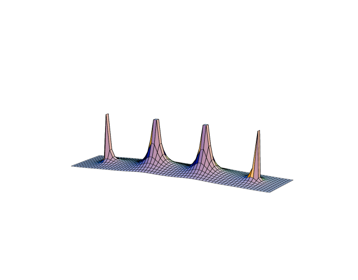
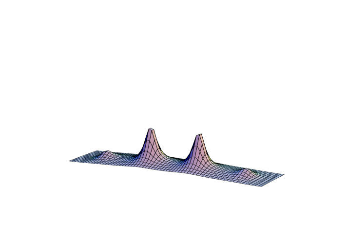
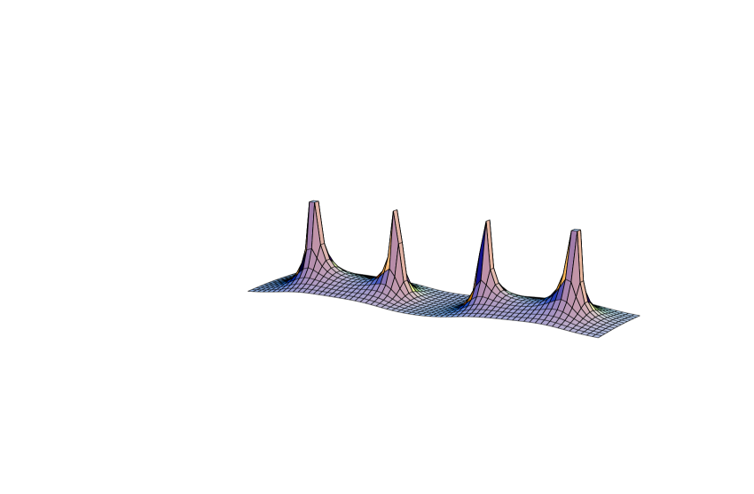
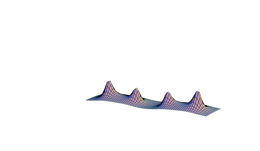
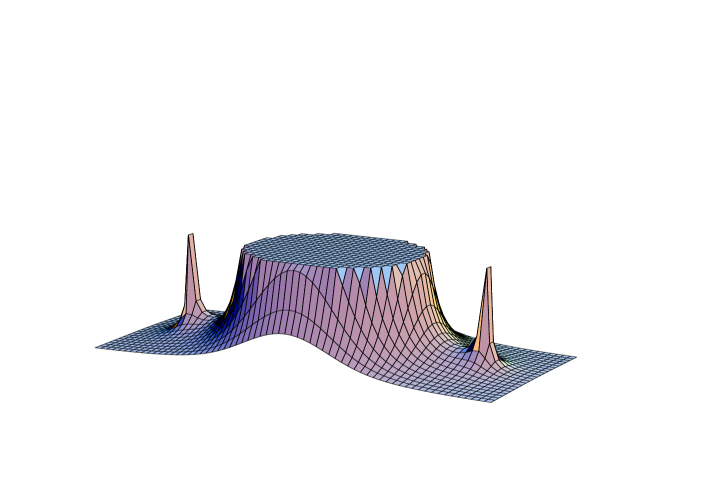
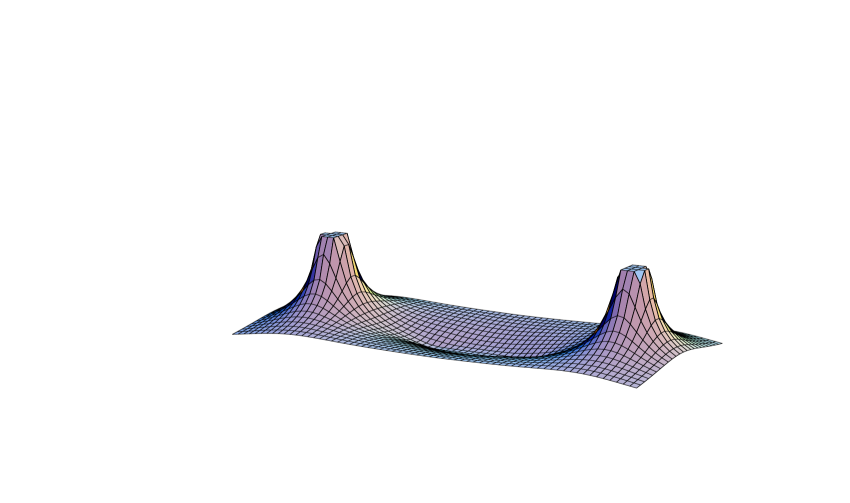
Figure 4: The two zero-mode densities at $z=\mu_{2}=1/4$ (same configuration as Fig. 3). The bipole zero-mode (right) is at 5 times the vertical scale of the second zero-mode (left). Top for the high temperature limit and bottom for finite temperature ($\beta=1$).

Figure 5: The two zero-mode densities for Eq. (41) with the order of $y_{1}^{(2)}$ and $y_{2}^{(1)}$ interchanged. The second zero-mode (left) is at the same scale, whereas the bipole zero-mode (right) has its vertical scale magnified by a factor 10, compared to Fig. 5.

the constraint on the alternating order of oppositely charged constituents, by smoothly deforming from $y_{2}^{(1)}<y_{1}^{(2)}$ to $y_{2}^{(1)}>y_{1}^{(2)}$. Under this deformation, both $\hat{\Psi}^{(1)}$ and $\hat{\Psi}^{(2)}$ remain zero-mode solutions of the Dirac equation, and $A_{\mu}$ remains a self-dual abelian gauge field. We now have a Dirac string for $y_{1}^{(2)}<x_{3}<y_{2}^{(1)}$ of double the usual strength ($\phi_{\rm{ff}}^{-1}$ behaving as $x_{\perp}^{4}$ as opposed to $x_{\perp}^{2}$), where the second zero-mode density diverges, as illustrated in Fig. 5. This is because $\phi_{(2)}$ will no longer be constant on the double Dirac string. The bipole zero-mode, on the other hand, remains well defined. It actually vanishes identically on the double Dirac string (cmp. Fig. 1 of Ref. [21]), and no longer “sees” the two inner self-dual Dirac monopoles.

It would be interesting if one could formulate an index theorem for these abelian field configurations with singularities, but this will not be straightforward as our analysis shows. It is yet another subtlety in describing the monopole content of non-abelian gauge fields. Developing a better understanding of these constraints, that affect the long range properties of configurations, is our main motivation for these studies.

5 Appearance of conserved quantities

Our analysis has shown that in all cases, as long as $z$ stays away from the impurities, the zero-mode density is exponentially localized to the cores of the constituents in the far field limit. The sizes of the monopole cores shrink to zero in the high temperature limit (with masses scaling proportional with the temperature), therefore we expect

$${\cal{V}}_{m}(\vec{x})\equiv(4\pi)^{-1}{\rm Tr}\left(R_{m}^{-1}(z)\right),$$ (44)

cmp. Eqs. 11 and 26, to be harmonic almost everywhere except for singularities tracing the cores of type $m$ monopoles for $z\in(\mu_{m},\mu_{m+1})$. Since the caloron gauge field does not depend on $z$, this interpretation requires ${\cal{V}}_{m}$ not to depend on $z$. The trace in Eq. (44) is necessary to remove any $z$ dependence due to the fact that the basis of zero-modes is only defined up to a – possibly $z$ dependent – unitary transformation. All this is obviously true when $\vec{R}(z;\vec{x})$ is piecewize constant, as for $k=1$ and for the class of axially symmetric solutions of Ref. [11]. In this case the zero-mode density in the high temperature limit reduces to the sum of $k$ delta function, located at the appropriate constituent monopole locations.

To show that ${\cal{V}}_{m}$ is independent of $z$, even when $\vec{R}(z,\vec{x})$ is not piecewize constant we solve the Riccati equation, Eq. (20), iteratively in $1/|\vec{x}|$ and obtain the multipole expansion for ${\cal{V}}_{m}(\vec{x})$. We can then use the Nahm equation for $\hat{A}_{j}(z)$ to check if every moment of this expansion is independent of $z$. We restrict our attention to the region between $\mu_{m}$ and $\mu_{m+1}$ and perform a rotation $U(\hat{x})$

$$Y_{i}(z)\equiv U_{ij}(\hat{x})\hat{g}(z)\frac{\hat{A}_{j}(z)}{2\pi i}\hat{g}^{\dagger}(z),\quad U(\hat{x})=\pmatrix{\sin(\theta)\cos(\varphi)&\sin(\theta)\sin(\varphi)&\hphantom{-}\cos(\theta)\cr\cos(\theta)\cos(\varphi)&\cos(\theta)\sin(\varphi)&-\sin(\theta)\cr-\sin(\varphi)&\cos(\varphi)&0\cr},$$ (45)

with $(\theta,\varphi)$ defined such that $U_{1j}=\hat{x}_{j}\equiv x_{j}/|\vec{x}|$ (the dependence of $\vec{Y}(z)$ on $\hat{x}$ will always be implicitly assumed). This leaves rotations around $\hat{x}$ as a remaining freedom, which we will make use of later. For the axially symmetric solutions discussed in Sect. 4, $\vec{Y}(z)=U(\hat{x})\vec{Y}_{m}$, cmp. Eq. (34).

The Nahm equation, which is invariant under rotations, is equivalent to (working in the gauge where $\hat{A}_{0}$ is constant, removed by the gauge transformation with $\hat{g}(z)$)

$${\frac{d}{dz}}Y_{i}(z)=-\pi i\varepsilon_{ijk}[Y_{j}(z),Y_{k}(z)].$$ (46)

We introduced $\vec{Y}(z)$ in Eq. (45) such that

$$\vec{R}(z;\vec{x})^{2}={\Eins}_{k}|\vec{x}|^{2}-2|\vec{x}|Y_{1}(z)+\vec{Y}^{\,2}(z),$$ (47)

has a simple form. Writing

$$R_{m}^{\pm}(z)^{2}\equiv{\Eins}_{k}|\vec{x}|^{2}-|\vec{x}|Q_{\pm}(z;|\vec{x}|^{-1}),$$ (48)

we can now formulate the Riccati equation, Eq. (20), in terms of $\vec{Y}(z)$ and $Q_{\pm}(z;|\vec{x}|^{-1})$,

$${\Eins}_{k}-\frac{Q_{\pm}(z;|\vec{x}|^{-1})}{|\vec{x}|}={\Eins}_{k}-2\frac{Y_{1}(z)}{|\vec{x}|}+\frac{\vec{Y}^{\,2}(z)}{|\vec{x}|^{2}}\pm\frac{1}{2\pi|\vec{x}|}{\frac{d}{dz}}\sqrt{{\Eins}_{k}-\frac{Q_{\pm}(z;|\vec{x}|^{-1})}{|\vec{x}|}},$$ (49)

which can be solved by iteration, expanding in powers of $1/|\vec{x}|$, something that is easily automated. We used the algebraic program FORM [26] for its superior memory management and speed to push this calculation to a high order. We find for the first few terms (also easily obtained by hand),

$$R_{m}^{\pm}(z)/|\vec{x}| = {\Eins}_{k}-Y_{1}/|\vec{x}|+{\scriptstyle{{1\over 2}}}(Y_{2}^{2}+Y_{3}^{2}\pm i[Y_{3},Y_{2}])/|\vec{x}|^{2}+$$

$${\scriptstyle{{1\over 2}}}(Y_{2}Y_{1}Y_{2}+Y_{3}Y_{1}Y_{3}\mp iY_{2}Y_{1}Y_{3}\pm iY_{3}Y_{1}Y_{2})/|\vec{x}|^{3}+\ldots$$

where the $z$ dependence of $Y_{j}(z)$ is suppressed for ease of notation and any derivatives with respect to $z$ are eliminated with the help of the Nahm equation, Eq. (46). We substitute this expansion in Eq. (44), with $R_{m}(z)={\scriptstyle{{1\over 2}}}(R_{m}^{+}(z)+R_{m}^{-}(z))$, from which we obtain its multipole expansion. The first few terms are

$${\cal{V}}_{m}(\vec{x})=\frac{1}{4\pi|\vec{x}|}{\rm Tr}\left({\Eins}_{k}+Y_{1}/|\vec{x}|+{\scriptstyle{{1\over 2}}}(3Y_{1}^{2}-\vec{Y}^{\,2})/|\vec{x}|^{2}+{\scriptstyle{{1\over 2}}}Y_{1}(5Y_{1}^{2}-3\vec{Y}^{\,2})/|\vec{x}|^{3}+\ldots\right).$$ (51)

A number of checks can be performed on this result. First of all ${\cal{V}}_{m}$ and $Q_{\pm}$ are invariant under any rotation among $Y_{2}$ and $Y_{3}$, ${\cal{V}}_{m}$ is real and $Q_{\pm}$ are hermitian, as should be. By construction, cmp. Eqs. (11), (26) and (44),

$$\sum_{a=1}^{k}\hat{\Psi}_{z}^{a}(x)^{\dagger}\hat{\Psi}_{z}^{a}(x)=-\partial_{i}^{2}{\cal{V}}_{m}(\vec{x}),\quad z\in(\mu_{m},\mu_{m+1})$$ (52)

in the far field limit, and one verifies that this integrates to $k$, as required by the proper normalization of the zero-modes. But most importantly, we verify with the help of the Nahm equation, Eq. (46), that ${\frac{d}{dz}}{\cal{V}}_{m}=0$ to the order given (whereas in general neither $R^{\pm}_{m}(z)$, nor ${\rm Tr}(R_{m}(z))$ are constant). For the dipole term this is immediate, since ${\frac{d}{dz}}{\rm Tr}Y_{1}=-2\pi i{\rm Tr}[Y_{2},Y_{3}]=0$. For the quadrupole term we have ${\frac{d}{dz}}{\rm Tr}(3Y_{1}^{2}-\vec{Y}^{\,2})=-4\pi i{\rm Tr}(3Y_{1}[Y_{2},Y_{3}]-\varepsilon_{ijk}Y_{i}Y_{j}Y_{k})=0$, using the cyclic property of the trace, etc. Note that ${\rm Tr}\hat{A}_{i}(z)$ plays a special role. It corresponds to the $U(1)$ part of the $U(k)$ Nahm gauge field, and therefore decouples in the Nahm equations. As is obvious from the definition of $\vec{R}(z;\vec{x})$, Eq. (14), it can actually be absorbed in a shift of $\vec{x}$. Therefore, where this simplifies matters we may assume $\vec{Y}(z)$ to be traceless.

Finally we check, as conjectured above, that each of the terms is harmonic. For this we have to note that $\vec{Y}(z)$ depends on $\vec{x}$ through the rotation $U(\hat{x})$, see Eq. (45). In the expression for ${\cal{V}}_{m}(\vec{x})$ the $\vec{x}$ dependence is easily recovered since $\vec{Y}^{\,2}$ is independent of $\vec{x}$ and $Y_{1}(z)=\hat{g}(z)\hat{A}_{j}(z)\hat{g}^{\dagger}(z)x_{j}/(2\pi i|\vec{x}|)$. It is now straightforward to verify that each term is harmonic. When $k=1$ we may use that $Y_{1}=\hat{x}\cdot\vec{y}_{m}$ is no longer a matrix, and one indeed finds ${\cal{V}}_{m}(\vec{x})$ in Eq. (51) to be the multipole expansion for $(4\pi|\vec{x}-\vec{y}_{m}|)^{-1}$ for that case. Since this is harmonic (for $\vec{x}\neq\vec{y}_{m}$), each term in the multipole expansion of ${\cal{V}}_{m}(\vec{x})$ has to be harmonic. For arbitrary $k$ and $\vec{Y}(z)$ we have checked these properties to order $|\vec{x}|^{-14}$ in the multipole expansion.

From now on we take charge 2. In this case there are 5 independent conserved quantities that characterize the solutions of the Nahm equation on a given interval $z\in[\mu_{m},\mu_{m+1}]$, apart from the 3 translational degrees of freedom contained in ${\rm Tr}\hat{A}_{i}(z)$. They are given by the entries of the traceless and symmetric matrix $M$,

$$M_{ij}\equiv-{\scriptstyle{{1\over 2}}}\left({\rm Tr}(\hat{A}_{i}(z)\hat{A}_{j}(z))-{\scriptstyle{{1\over 3}}}\delta_{ij}{\rm Tr}(\hat{A}_{k}(z)\hat{A}_{k}(z))\right).$$ (53)

One easily checks with the Nahm equation that this is conserved, as for the quadrupole term considered above. Although not needed here, it is known [7] that for any $k$ a solution to the Nahm equation implies $\det(y_{j}\hat{A}_{j}(z)-2\pi iy_{j}x_{j})$ is constant, provided $\vec{y}\in C^{3}$, with $y_{j}^{2}=0$. Indeed, for $k=2$ and $\vec{x}=\vec{0}$, using that $\det(y_{j}\hat{A}_{j}(z))=-{\scriptstyle{{1\over 2}}}{\rm Tr}(y_{j}\hat{A}_{j}(z))^{2}$, this is equivalent to $M$ being constant if and only if $y_{j}^{2}=0$. Since $M$ gives all the independent invariants, it should be possible to express ${\cal{V}}_{m}(\vec{x})$ in terms of $M$ and $\vec{x}$. Considerable simplifications occur, because we can write

$$\hat{A}_{j}(z)\equiv i{\cal{A}}_{ja}(z)\hat{g}^{\dagger}(z)\tau_{a}\hat{g}(z)$$ (54)

(absorbing the trace part in a shift of $\vec{x}$), and use $\tau_{a}\tau_{b}=\delta_{ab}{\Eins}_{2}+i\varepsilon_{abc}\tau_{c}$ to reduce the matrix products to scalar products, ${\cal{A}}_{ia}(z){\cal{A}}_{ja}(z)=M_{ij}+{\scriptstyle{{1\over 3}}}\delta_{ij}{\cal{A}}^{2}_{ka}(z)$. We do indeed find that ${\cal{V}}_{m}(\vec{x})$ is a function of $M$ and $\vec{x}$ only,

$${\cal{V}}_{m}(\vec{x})=\frac{1}{2\pi|\vec{x}|}\left(1+\frac{3}{2|\vec{x}|^{2}}\hat{M}_{11}(\hat{x})+{\cal{O}}(|\vec{x}|^{-4})\right).$$ (55)

where for convenience we introduced

$$\hat{M}_{ij}(\hat{x})=\frac{1}{4\pi^{2}}\left(U(\hat{x})MU^{-1}(\hat{x})\right)_{ij}={\scriptstyle{{1\over 2}}}{\rm Tr}\left(Y_{i}(z)Y_{j}(z)-{\scriptstyle{{1\over 3}}}\delta_{ij}\vec{Y}^{\,2}(z)\right).$$ (56)

We performed the multipole expansion for charge 2 to order $|\vec{x}|^{-21}$. Only the odd orders appear, because $\vec{Y}(z)$ is assumed to be traceless. In appendix B we give the term of order 21, and show how from this all lower order multipole coefficients can be recovered.

6 Exact results for charge 2

In this section we will construct $SU(2)$ charge 2 solutions for which $\vec{R}(z;\vec{x})$ is not piecewize constant and analyse the localization of the fermion zero-modes in the far field limit. We already saw in Sect. 5 that on each interval $(\mu_{m},\mu_{m+1})$ we have information on the zero-mode density, Eq. (52), in terms of 8 parameters. Three of these are associated with ${\rm Tr}\vec{Y}(z)$, which give the center of mass coordinates for the constituents of type $m$. Of the other 5, given by the $3\times 3$ traceless symmetric matrix $M$, 3 are associated to a rotation ${\cal{R}}$ that diagonalizes $M$, whereas the remaining 2 parameterize the eigenvalues of $M$. They will give a scale ($D$) and shape (${\bf k}$) parameter, see below.

6.1 Solutions to the Nahm equation

Explicit solutions in terms of Jacobi elliptic functions were first considered in the context of $SU(2)$ charge 2 monopoles [27, 28]. These solutions can be adopted for the calorons provided the appropriate boundary conditions, read off from Eq. (15), are implemented. In terms of the $3\times 3$ matrix ${\cal{A}}_{ia}(z)$ defined in Eq. (54), the Nahm equation becomes (away from $z=\mu_{m}$)

$$\frac{1}{2}{\frac{d}{dz}}{\cal{A}}^{t}(z)=\det({\cal{A}}(z)){\cal{A}}^{-1}(z),$$ (57)

from which we find

$$\frac{1}{4}{\frac{d}{dz}}\left({\cal{A}}(z){\cal{A}}^{t}(z)\right)={\Eins}_{3}\det{\cal{A}}(z)={\Eins}_{3}\sqrt{\det\left({\cal{A}}(z){\cal{A}}^{t}(z)\right)}.$$ (58)

The traceless part of ${\cal{A}}(z){\cal{A}}^{t}(z)$ is therefore independent of $z$, once again verifying that $M={\cal{A}}(z){\cal{A}}^{t}(z)-{\scriptstyle{{1\over 3}}}{\Eins}_{3}{\rm Tr}({\cal{A}}(z){\cal{A}}^{t}(z))$ is constant. Here we are, however, interested in the equation for the trace part

$${\frac{d}{dz}}F(z)=4\sqrt{\det\left(F(z){\Eins}_{3}+M\right)},\quad F(z)\equiv{\scriptstyle{{1\over 3}}}{\rm Tr}\left({\cal{A}}(z){\cal{A}}^{t}(z)\right).$$ (59)

When we diagonalize $M$ with a suitable rotation ${\cal{R}}$, $M={\cal{R}}{\rm diag}(c_{1},c_{2},c_{3}){\cal{R}}^{t}$, fixing ${\cal{R}}$ such that $c_{2}\leq c_{1}\leq c_{3}$ (note that in addition $c_{1}+c_{2}+c_{3}={\rm Tr}M=0$), this can be cast in the form

$${\frac{d}{dz}}F(z)=4\sqrt{(F(z)+c_{1})(F(z)+c_{2})(F(z)+c_{3})}.$$ (60)

Defining $F(z)+c_{i}={\scriptstyle{{1\over 4}}}D^{2}f_{i}^{2}(Dz)$ and introducing $D$ and ${\bf k}$ to parameterize the $c_{i}$,

$$D^{2}\equiv{\scriptstyle{{1\over 4}}}(c_{3}-c_{2}),\quad{\bf k}^{2}\equiv\frac{c_{3}-c_{1}}{c_{3}-c_{2}}\leq 1,$$ (61)

shows that the solution can be written in terms of the Jacobi elliptic functions

$$f_{1}(z)=\frac{{\bf k}^{\prime}}{cn_{\bf k}(z)},\quad f_{2}(z)=\frac{{\bf k}^{\prime}sn_{\bf k}(z)}{cn_{\bf k}(z)},\quad f_{3}(z)=\frac{dn_{\bf k}(z)}{cn_{\bf k}(z)},\quad{\bf k}^{\prime}\equiv\sqrt{1-{\bf k}^{2}}.$$ (62)

The overall sign of the functions $f_{i}(z)$ is chosen such that $df_{1}(z)/dz=f_{2}(z)f_{3}(z)$, and cyclic, such that in terms of these the most general solution of the Nahm equation is given by

$$\hat{A}_{j}(z;\vec{a},{\cal{R}},h,{\cal{D}},{\bf k})\equiv 2\pi i\hat{g}^{\dagger}(z)h^{\dagger}\Bigl{(}a_{j}{\Eins}_{2}+{\cal{D}}{\cal{R}}_{jb}f_{b}(Dz)\tau_{b}\Bigr{)}h\hat{g}(z),\quad{\cal{D}}\equiv(4\pi)^{-1}D,$$ (63)

where ${\cal{R}}$ is the rotation that diagonalizes $M$ and $h$ is a global gauge rotation (leaving ${\cal{A}}(z){\cal{A}}^{t}(z)$ invariant). In the $Sp(1)$ formalism for constructing $SU(2)$ calorons one requires $\hat{A}^{t}_{j}(z)=\hat{A}_{j}(-z)$, a property shared by $f_{b}(Dz)\tau_{b}$ for each $b$. Arranging $f_{2}(z)$ to be odd and $f_{1,3}(z)$ to be even in $z$ was the reason for choosing $c_{2}\leq c_{1}\leq c_{3}$.

We see that ${\bf k}^{\prime}=0$ (i.e. ${\bf k}=1$) recovers the case where $\vec{R}(z;\vec{x})$ is piecewize constant, for which ${\cal{V}}^{{\bf k}=1}_{m}(\vec{x})=(4\pi|\vec{x}-\vec{y}|)^{-1}+(4\pi|\vec{x}+\vec{y}|)^{-1}$, with $\vec{y}=(0,0,{\cal{D}})$ and $\pm\vec{y}$ the two locations of the equal charge constituents (the center of mass assumed to be zero), see Sect. 5. The combined zero-mode density in the far field limit is given by $-\partial_{i}^{2}{\cal{V}}_{m}(\vec{x})=\delta(\vec{x}-\vec{y})+\delta(\vec{x}+\vec{y})$, the sum of two delta-functions at these constituent locations. Actually, two point-like constituents necessarily implies ${\bf k}=1$. Comparing $3\hat{M}_{11}/(16\pi^{3}|\vec{x}|^{3})=3\sum_{j=1}^{3}c_{j}x_{j}^{2}/(16\pi^{3}|\vec{x}|^{5})$, see Eq. (56), with the quadrupole term for ${\cal{V}}^{{\bf k}=1}_{m}(\vec{x})$, $(2x_{3}^{2}-x_{2}^{2}-x_{1}^{2}){\cal{D}}^{2}/(4\pi|\vec{x}|^{5})$, one finds that $c_{1}=c_{2}$, which forces ${\bf k}=1$. It is in this context that we define $\vec{y}=\pm(0,0,{\cal{D}})$ as would-be constituent locations even when ${\bf k}\neq 1$. In which way we will approach point-like constituents when ${\bf k}\to 1$ will become clear in Sect. 6.3. So far we have studied the Nahm equation away from the “impurities”. We first want to convince ourselves that there are more general (not piecewize constant) solutions to the Nahm equation that describe calorons with non-trivial holonomy, for which we need to solve the boundary conditions at the “impurities”.

6.2 Matching at the impurities

We will consider here the case of $SU(2)$ charge 2 calorons in the symplectic representation, for which $\hat{A}_{j}(-z)=\hat{A}^{t}_{j}(z)$. This condition is preserved under the gauge transformation $\hat{g}(z)$ defined in Eq. (13), but requires us to further constrain $h$ appearing in Eq. (63) to be generated by $\tau_{2}$. It means that for $z\in[\mu_{1},\mu_{2}]$ the Nahm gauge field is given by $\hat{A}_{j}(z)=\hat{A}_{j}(z;\vec{a}^{(1)},{\cal{R}}^{(1)},e^{-\frac{i}{2}\theta^{(1)}\tau_{2}},{\cal{D}}^{(1)},{\bf k}^{(1)})$. For $z\in[\mu_{2},1+\mu_{1}]$ we use that periodicity of $\hat{A}_{j}(z)$ implies $\hat{A}_{j}(1-z)=\hat{A}_{j}(-z)=\hat{A}_{j}^{t}(z)$, such that $\hat{A}_{j}(z)=\hat{A}_{j}(z-{\scriptstyle{{1\over 2}}};\vec{a}^{(2)},{\cal{R}}^{(2)},e^{-\frac{i}{2}\theta^{(2)}\tau_{2}},{\cal{D}}^{(2)},{\bf k}^{(2)})$. This was studied before by Houghton and Kraan for trivial holonomy ($\mu_{2}=0$) [30], where one of the monopole types is massless. For general holonomy, the Nahm equation reduces at $z=\mu_{2}$ to (see Eq. (15))

$$\hat{A}_{j}(\mu_{2}-{\scriptstyle{{1\over 2}}};\vec{a}^{(2)},{\cal{R}}^{(2)},e^{-\frac{i}{2}\theta^{(2)}\tau_{2}},{\cal{D}}^{(2)},{\bf k}^{(2)})-\hat{A}_{j}(\mu_{2};\vec{a}^{(1)},{\cal{R}}^{(1)},e^{-\frac{i}{2}\theta^{(1)}\tau_{2}},{\cal{D}}^{(1)},{\bf k}^{(1)})=2\pi i\rho_{2}^{j}.$$ (64)

At $z=\mu_{1}=-\mu_{2}$, using $\hat{A}_{j}(-z)=\hat{A}_{j}(z)^{t}$, the same condition is found (one can check [11] that $\rho_{1}=-\rho_{2}^{t}$).

Figure 6: Plotting $|\Delta\vec{a}|$ versus $D$, Eq. (66), for ${\bf k}=0,$ 0.9, 0.99, 0.999 and 0.9999 (left to right).

A particularly simple solution is obtained for $\mu_{2}=1/4$ (equal mass constituents) by taking the same parameters in both intervals, up to a shift $\vec{a}$, ${\cal{D}}^{(m)}={\cal{D}}$, ${\bf k}^{(m)}={\bf k}$, ${\cal{R}}^{(m)}={\Eins}_{3}$ and $\theta^{(m)}=0$, collapsing Eq. (64) to

$$\vec{\rho}_{2}=\Delta\vec{a}{\Eins}_{2}-2(0,1,0)\tau_{2}{\cal{D}}{\bf k}^{\prime}\frac{sn_{\bf k}({\scriptstyle{{1\over 4}}}D)}{cn_{\bf k}({\scriptstyle{{1\over 4}}}D)},\quad\Delta\vec{a}\equiv\vec{a}^{(2)}-\vec{a}^{(1)}$$ (65)

This can be solved by taking $P_{2}={\scriptstyle{{1\over 2}}}({\Eins}_{2}+\tau_{2})$, $\zeta_{a}=\rho\exp(2\pi i\alpha_{a}\tau_{2})$, with $\alpha_{1}-\alpha_{2}=1/4$, which gives $\vec{\rho}_{2}^{\,ab}=-2\pi\rho^{2}P_{2}^{ab}(0,1,0)$, such that

$$\frac{D{\bf k}^{\prime}sn_{\bf k}({\scriptstyle{{1\over 4}}}D)}{2\pi cn_{\bf k}({\scriptstyle{{1\over 4}}}D)}(0,1,0)=-\Delta\vec{a}=\pi\rho^{2}(0,1,0).$$ (66)

For increasing $D$, $cn_{\bf k}({\scriptstyle{{1\over 4}}}D)$ will reach zero at ${\scriptstyle{{1\over 4}}}D=K({\bf k})$, the half-period. To keep $|\Delta\vec{a}|$ finite, ${\bf k}^{\prime}$ has to approach zero as well.

In Fig. 6 we plot $|\Delta\vec{a}|$ as a function of ${\bf k}$ and $D$, from which we confirm that, at fixed $|\Delta\vec{a}|$, ${\bf k}$ has to approach 1 to have well separated constituents. In this point-like limit, monopole constituents of type 1 are located at $(0,-{\scriptstyle{{1\over 2}}}\pi\rho^{2},\pm{\cal{D}})$ and those of opposite charge (type 2) at $(0,{\scriptstyle{{1\over 2}}}\pi\rho^{2},\pm{\cal{D}})$ (choosing the overall center of mass at the origin). This configuration has parallel magnetic moments and placing self-dual Dirac monopoles at the mentioned locations would give a gauge field in the bipole ansatz, Eq. (35). However, the abelian component of the gauge field coming from the above caloron can at best take the bipole form in the limit discussed. For ${\bf k}=1$ and ${\cal{D}}$ finite, $|\Delta\vec{a}|=0$, and one is left with two singular instantons (of zero size) at $(0,0,\pm{\cal{D}})$.

For this reason we now consider a class of solutions which contains regular axially symmetric solutions with ${\bf k}=1$. Again we take $\mu_{2}=1/4$, ${\cal{D}}^{(m)}={\cal{D}}$, ${\bf k}^{(m)}={\bf k}$, $\zeta_{a}=\rho\exp(2\pi i\alpha_{a}\tau_{2})$, but now with $\alpha_{2}=-\alpha_{1}\equiv\pi^{-1}\alpha$, $P_{2}={\scriptstyle{{1\over 2}}}(1+\tau_{3})$, $\theta^{(2)}=-\theta^{(1)}\equiv\theta$ and

$${\cal{R}}^{(2)}=\left({\cal{R}}^{(1)}\right)^{-1}=\pmatrix{\cos\varphi&0&\sin\varphi\cr 0&1&0\cr-\sin\varphi&0&\cos\varphi}.$$ (67)

One finds

$$\vec{\rho}_{2}^{\,ab}=-\pi\rho^{2}(-\sin\alpha\tau_{3},-\sin\alpha\tau_{2},\tau_{1}+\cos\alpha{\Eins}_{1})^{ab},$$ (68)

and Eq. (64) takes the following form

$$2{\cal{D}}(f_{1}({\scriptstyle{{1\over 4}}}D)\sin\theta\cos\varphi+f_{3}({\scriptstyle{{1\over 4}}}D)\cos\theta\sin\varphi)\tau_{3}+\Delta a_{1}{\Eins}_{2} = \pi\rho^{2}\sin\alpha\tau_{3}$$

$$-2{\cal{D}}f_{2}({\scriptstyle{{1\over 4}}}D)\tau_{2}+\Delta a_{2}{\Eins}_{2} = \pi\rho^{2}\sin\alpha\tau_{2}$$ (69)

$$-2{\cal{D}}(f_{1}({\scriptstyle{{1\over 4}}}D)\cos\theta\sin\varphi+f_{3}({\scriptstyle{{1\over 4}}}D)\sin\theta\cos\varphi)\tau_{1}+\Delta a_{3}{\Eins}_{2} = -\pi\rho^{2}(\tau_{1}+\cos\alpha{\Eins}_{2}).$$

This can be simplified to

$${\cal{D}}\sin(\theta-\varphi)\Bigl{(}f_{3}({\scriptstyle{{1\over 4}}}D)-f_{1}({\scriptstyle{{1\over 4}}}D)\Bigr{)}={\scriptstyle{{1\over 2}}}\pi\rho^{2}(1-\sin\alpha), \Delta\vec{a}=-\pi\rho^{2}\cos\alpha(0,0,1),$$ (70)

$${\cal{D}}\sin(\theta+\varphi)\Bigl{(}f_{3}({\scriptstyle{{1\over 4}}}D)+f_{1}({\scriptstyle{{1\over 4}}}D)\Bigr{)}={\scriptstyle{{1\over 2}}}\pi\rho^{2}(1+\sin\alpha), {\cal{D}}f_{2}({\scriptstyle{{1\over 4}}}D)=-{\scriptstyle{{1\over 2}}}\pi\rho^{2}\sin\alpha,$$

It gives a three parameter family of solutions with would-be point-like constituents at

$$\vec{y}_{m}^{\,(j)}=((-1)^{j}{\cal{D}}\sin\varphi,0,(-1)^{m+j}{\cal{D}}\cos\varphi-(-1)^{m}{\scriptstyle{{1\over 2}}}\rho^{2}\cos\alpha).$$ (71)

To have an exact point-like far field limit we need to impose ${\bf k}=1$, implying $\sin\alpha=0$ and $\cos\theta\sin\varphi=0$. The first possibility is that $\cos\theta=0$, for which $|\cos\varphi|{\cal{D}}={\scriptstyle{{1\over 2}}}\rho^{2}$. One finds two constituents of opposite charge to coincide. Such a solution describes a singular (zero-size) instanton on top of a smooth caloron. Excluding this singular case we are left with the choice $\sin\varphi=0$, for which $|\sin\theta|{\cal{D}}={\scriptstyle{{1\over 2}}}\rho^{2}$. We now find axially symmetric solutions with constituent locations at

$$\vec{y}_{m}^{\,(j)}=\mp{\scriptstyle{{1\over 2}}}\pi\rho^{2}\left((-1)^{m}+(-1)^{j}|\sin\theta|^{-1}\right)(0,0,1),$$ (72)

where the overall sign comes from the fact that $\cos\alpha=\pm 1$. For $\cos\theta\neq 0$, all constituents are now separated from each other, giving a regular solution. Both cases were already studied in Ref. [11], based on assuming that $\vec{\rho}_{2}$ is one dimensional (cmp. Sect. 4). It can be shown that for $SU(2)$ exact point-like constituents, ${\bf k}^{(1)}={\bf k}^{(2)}=1$, forces $\vec{\rho}_{2}$ to be one dimensional for any choice of the remaining parameters.

Figure 7: On the left we plot ${\bf k}$ versus $\rho$ for $\alpha=0$ (${\bf k}\equiv 1$), $\alpha=-\pi/100$ and $\alpha=-\pi/2$ (giving the lower bound for ${\bf k}$ at fixed $\rho$). On the right are shown the locations, Eq. (71), of monopoles and antimonopoles (fat vs. thin curves) in the $1,3$-plane for $\rho=1/4$, by varying $\alpha$ from $-\pi$ (indicated by the arrows) to 0.

Nevertheless, when $\sin\alpha\neq 0$, insisting as before that equal charge constituents are well separated, while keeping the centers of mass of these pairs at a fixed distance $\pi\rho^{2}\cos\alpha$, one forces ${\bf k}\to 1$ while increasing ${\cal{D}}$, and hence approximate point-like constituents. We will illustrate this behavior for $\theta=\pi/4$. In Fig. 7 we plot for a typical value of $\rho$ the constituent locations as given by Eq. (71), varying $\alpha$ between $-\pi$ and 0 (given $\rho$, $\alpha$ and $\theta$, one can use Eq. (70) to solve for $\varphi$, ${\cal{D}}$ and ${\bf k}$). We also plot ${\bf k}$ as a function of $\rho$ for some values of $\varphi$, showing the rapid uniform approach to ${\bf k}=1$. The asymptotic behavior for $\alpha=-\pi/2$ is determined by

$${\bf k}^{\prime}=\frac{4\exp(-D/4)}{3+2\sqrt{2}}\left(1+{\cal{O}}({\bf k}^{\prime 2})\right),\quad D=4\sqrt{2}\pi^{2}\rho^{2}\left(1+{\cal{O}}({\bf k}^{\prime 2})\right).$$ (73)

It is also interesting to inspect $\hat{A}_{i}(z)$ in the limit ${\bf k}\to 1$ (or ${\cal{D}}\to\infty$), to understand to which extent we retrieve the piecewize constant behavior of $\vec{R}(z;\vec{x})$, on which the point-like limit is based. For this we plot $f_{i}(D({\bf k})z)$ in Fig. 8, which apart from fixed rotations and an overall factor ${\cal{D}}$ would represent the constituent locations. Since ${\cal{D}}({\bf k})/(\pi\rho^{2})$ approaches $\sqrt{2}$ for ${\bf k}\to 1$, it means we normalize the constituent locations with respect to height of the jumps in the Nahm data. At the impurities ($z=\pm 1/4$) we therefore expect $f_{i}(D({\bf k})z)$ to go to a fixed value. The plotted cases, $1-{\bf k}=10^{-4}$, $D({\bf k})=15.53$ (left) and $1-{\bf k}=10^{-8}$, $D({\bf k})=33.95$ (right), clearly demonstrate how in the bulk $f_{3}\to 1$ and $f_{1,2}\to 0$, but that they differ at $z=\pm 1/4$, to accommodate the discontinuities of the Nahm equation at the impurities. The cross-over from bulk behavior to the impurity values scales as $D^{-1}$, and is only absent for axially symmetric solutions.

$f_{3}$
                                                               $f_{1}$
                                                               $f_{2}$

Figure 8: Plots of $f_{j}(D({\bf k})z)$ for $z\in[-{\scriptstyle{{1\over 4}}},{\scriptstyle{{1\over 4}}}]$ at ${\bf k}=1-10^{-4}$ (left) and ${\bf k}=1-10^{-8}$ (right), illustrating the approach to the point-like limit ${\bf k}\to 1$.

6.3 Extended structure

When $\vec{R}(z;\vec{x})$ is not piecewize constant, it is not clear what plays the role of the constituent locations. We therefore do expect some extended structure for ${\bf k}\neq 1$. For this reason we now come back to analysing ${\cal{V}}_{m}(\vec{x})=(4\pi)^{-1}{\rm Tr}R_{m}^{-1}(z)$ in more detail. Quite remarkably, the discussion in Sect. 5 implies that the result for ${\bf k}=0$ can be obtained from that at ${\bf k}=1$. For this we may use the symmetry $c_{2}\leftrightarrow c_{3}$, which leaves ${\cal{V}}_{m}(\vec{x})$ invariant, apart from interchanging $x_{2}$ and $x_{3}$ ($\hat{M}$ is left unchanged when absorbing the rotation ${\cal{R}}$ that interchanges $c_{2}$ and $c_{3}$ in $U$, see Eq. (56)). With the definitions of $D=4\pi{\cal{D}}$ and ${\bf k}$ in Eq. (61) one finds that this implies ${\cal{D}}^{2}\to-{\cal{D}}^{2}$ and ${\bf k}\to{\bf k}^{\prime}$. Therefore,

$${\bf k}=0:\quad{\cal{V}}_{m}(\vec{x})=\frac{\sqrt{2}\sqrt{|\vec{x}|^{2}-{\cal{D}}^{2}+\sqrt{(|\vec{x}|^{2}-{\cal{D}}^{2})^{2}+4{\cal{D}}^{2}x_{2}^{2}}}}{4\pi\sqrt{(|\vec{x}|^{2}-{\cal{D}}^{2})^{2}+4{\cal{D}}^{2}x_{2}^{2}}}.$$ (74)

For this we use that the ${\bf k}=1$ result, ${\cal{V}}_{m}(\vec{x})=(4\pi|\vec{x}-\vec{y}|)^{-1}+(4\pi|\vec{x}+\vec{y}|)^{-1}$, with $\vec{y}={\cal{D}}(0,0,1)$, can be rewritten in the form of Eq. (74) by changing the sign of ${\cal{D}}^{2}$ and interchanging $x_{2}$ and $x_{3}$. In some sense we may say that the result for ${\bf k}=0$ describes point-like constituents that have moved into a complex direction. We note that Eq. (74) is singular on the ring $x_{2}=0$, $|\vec{x}|^{2}={\cal{D}}^{2}$, i.e. on the circle of radius $|{\cal{D}}|$ in the $1,3$-plane. But there is more of a surprise: the $x_{2}$ derivative is discontinuous on the disk bounded by the ring (away from the disc the function is smooth and harmonic), ${\cal{V}}_{m}(\vec{x})=(2\pi)^{-1}|{\cal{D}}x_{2}|/({\cal{D}}^{2}-r^{2})^{3/2}(1+{\cal{O}}(x_{2}^{2}))$, with $r^{2}\equiv x_{1}^{2}+x_{3}^{2}$. This implies indeed an extended structure, with singularities on the entire disk. Before showing how to deal with this singularity structure we consider general values of ${\bf k}$.

As we have seen in Sect. 5, ${\rm Tr}R_{m}^{-1}(z)$ is conserved as a consequence of the Nahm equation. Using for $R_{m}^{\pm}(z)$ the Riccati equation, Eq. (20), the fact that ${\rm Tr}R_{m}^{-1}(z)=2{\rm Tr}(R_{m}^{+}(z)+R_{m}^{-}(z))^{-1}$ is independent of $z$ imposes a severe constraint. We make use of this by expanding $R_{m}^{\pm}(z)$ as a Taylor series in $z$. The Taylor coefficients can be expressed in terms of the initial conditions $R_{m}^{\pm}(0)$, through the explicit solution of $\hat{A}_{j}(z)$, Eq. (63) (we make use of the invariance under translations and rotations to put $\vec{a}=\vec{0}$, $h={\Eins}_{2}$ and ${\cal{R}}={\Eins}_{3}$, as in Sect. 5). We thus obtain the Taylor series for ${\rm Tr}R_{m}^{-1}(z)$, of which all coefficients should vanish except for the 0th order. This gives a set of algebraic equations for the initial conditions, $R_{m}^{\pm}(0)$, encoded in $X_{\mu}$ and $\tilde{X}_{\mu}$ through

$$R_{m}(0)={\scriptstyle{{1\over 2}}}(R_{m}^{+}(0)+R_{m}^{-}(0))\equiv{\cal{D}}(X_{0}{\Eins}_{2}+X_{j}\tau_{j}),\quad{\scriptstyle{{1\over 2}}}(R_{m}^{+}(0)-R_{m}^{-}(0))\equiv{\cal{D}}(\tilde{X}_{0}{\Eins}_{2}+\tilde{X}_{j}\tau_{j}),$$ (75)

Note that ${\cal{D}}$ enters as an overall scale factor, cmp. Eq. (63), such that

$${\cal{V}}_{m}(\vec{x})=\frac{1}{4\pi}{\rm Tr}R_{m}^{-1}(0)=\frac{1}{2\pi{\cal{D}}}\tilde{\cal{V}}({\cal{D}}\vec{x}),\quad\tilde{\cal{V}}={\scriptstyle{{1\over 2}}}{\rm Tr}\left(\frac{1}{X_{0}+X_{j}\tau_{j}}\right)=\frac{X_{0}}{X_{0}^{2}-X_{j}^{2}}.$$ (76)

Dependence on the coordinates and on ${\bf k}$ is mostly left implicit. The system of equations is of course hugely overdetermined, and some amount of good fortune was required in that the first 11 orders in the Taylor expansion were sufficient to solve for $X_{\mu}$ and $\tilde{X}_{\mu}$. Quite remarkably these imply that $\tilde{X}_{0}=\tilde{X}_{1}=\tilde{X}_{3}=X_{2}=0$, which considerably simplifies the task of solving for the remaining 4 variables. We found that

$$\delta\equiv X_{0}^{2}-X_{1}^{2}-X_{3}^{2}-\tilde{X}_{2}^{2}$$ (77)

satisfies the cubic equation

$$\hskip-25.60747pt(2-{\bf k}^{2}){\bf k}^{4}+4{\bf k}^{2}(x_{1}^{2}-x_{3}^{2})-{\bf k}^{4}(3x_{1}^{2}-x_{2}^{2}-x_{3}^{2})+\left((2-{\bf k}^{2})(3x_{1}^{2}-x_{2}^{2}+x_{3}^{2})-4x_{1}^{2}\right)|\vec{x}|^{2}$$

$$\hskip-14.22636pt-|\vec{x}|^{6}-\left({\bf k}^{4}+2{\bf k}^{2}(x_{1}^{2}-x_{2}^{2}-x_{3}^{2})+4x_{2}^{2}+|\vec{x}|^{4}\right)\delta+\left({\bf k}^{2}-2+|\vec{x}|^{2}\right)\delta^{2}+\delta^{3}=0,$$ (78)

whereas $X_{1}/X_{0}$, $X_{3}/X_{0}$ and $\tilde{X}_{2}$ can be solved for in terms of $\delta$,

$$X_{1}/X_{0} = \frac{|\vec{x}|^{4}-\delta^{2}+2({\bf k}^{\prime 2}(\delta-2x_{1}^{2})+x_{1}^{2}+x_{2}^{2}-x_{3}^{2})+(2-{\bf k}^{2}){\bf k}^{2}}{4x_{1}{\bf k}^{\prime}{\bf k}^{2}}$$

$$X_{3}/X_{0} = \frac{|\vec{x}|^{4}-\delta^{2}+2(\delta-2x_{3}^{2}-{\bf k}^{\prime 2}(x_{1}^{2}-x_{2}^{2}-x_{3}^{2}))-(2-{\bf k}^{2}){\bf k}^{2}}{4x_{3}{\bf k}^{2}}$$

$$\tilde{X}_{2} = \frac{|\vec{x}|^{4}-\delta^{2}+2{\bf k}^{2}(x_{1}^{2}-x_{2}^{2}-x_{3}^{2})+4x_{2}^{2}+{\bf k}^{4}}{4x_{2}{\bf k}^{\prime}}.$$ (79)

Therefore, $\tilde{\cal{V}}^{2}$ is a rational function of $\delta$, $\vec{x}$ and $k$,

$$\tilde{\cal{V}}^{2}=\frac{1}{(\delta+\tilde{X}_{2}^{2})(1-X_{1}^{2}X_{0}^{-2}-X_{3}^{2}X_{0}^{-2})},$$ (80)

and the proper root of the cubic equation for $\delta$ to use is fixed by $\tilde{\cal{V}}\to 1/|\vec{x}|$. Indeed, the asymptotic expansion for $\delta$,

$$\delta=|\vec{x}|^{2}\left(1+\frac{2x_{2}^{2}+{\bf k}^{2}(x_{1}^{2}-x_{2}^{2}-x_{3}^{2})}{|\vec{x}|^{4}}+\ldots\right),$$ (81)

reproduces the multipole expansion of $\tilde{\cal{V}}$. This was verified to the 21 orders given in Eq. (104). On general grounds it can be argued, since $\delta$ satisfies a cubic equation, that $\tilde{\cal{V}}^{2}$ has to satisfy a cubic equation as well. Its coefficients (polynomials in ${\bf k}$ and $\vec{x}$) are somewhat lengthy, and therefore not reproduced here, in part because we will shortly present an exact integral equation for ${\cal{V}}_{m}(\vec{x})$, valid for any ${\bf k}$. The exact results for ${\bf k}=0$ and ${\bf k}=1$ is most easily recovered from the cubic equation for $\tilde{\cal{V}}^{2}$, but the integral representation will be valid for these two cases as well.

Like for ${\bf k}=0$, we find that ${\cal{V}}_{m}(\vec{x})$ is harmonic everywhere except on a disk, now bounded by an ellipse with major and minor axes ${\cal{D}}$, resp. ${\bf k}^{\prime}{\cal{D}}$. On this disk the function vanishes, satisfying in the direction perpendicular to the disk the expansion ${\cal{V}}_{m}(\vec{x})=(2\pi)^{-1}{\bf k}^{\prime}|{\cal{D}}x_{2}|/({\cal{D}}^{2}{\bf k}^{\prime 2}-x_{1}^{2}-{\bf k}^{\prime 2}x_{3}^{2})^{3/2}(1+{\cal{O}}(x_{2}^{2}))$ (cmp. the discussion above, for ${\bf k}=0$). By introducing the “polar” coordinates $(x_{1},x_{3})=({\bf k}^{\prime}r\cos\varphi,r\sin\varphi)$, in terms of which the ellipse at the boundary of the disk is characterized by $r={\cal{D}}$, this can be written as ${\cal{V}}_{m}(\vec{x})=(2\pi{\bf k}^{\prime})^{-1}|{\cal{D}}x_{2}|/({\cal{D}}^{2}-r^{2})^{3/2}(1+{\cal{O}}(x_{2}^{2}))$. Care is required to deal correctly with the behavior at the edge of the disk when computing the Laplacian. We find

$$-\partial_{i}^{2}{\cal{V}}_{m}(\vec{x})=-\delta(x_{2})\frac{{\cal{D}}}{\pi r{\bf k}^{\prime}}\frac{\partial}{\partial r}\frac{\theta({\cal{D}}-r)}{\sqrt{{\cal{D}}^{2}-r^{2}}},$$ (82)

with $\theta({\cal{D}}-r)$ the step function, giving the following integral representation

$${\cal{V}}_{m}(\vec{x})=\frac{1}{2\pi|\vec{x}|}+\frac{{\cal{D}}}{4\pi^{2}}\int_{0}^{2\pi}\!\!\!\!\!d\varphi\int_{0}^{\cal{D}}\!\!\!\frac{dr}{\sqrt{{\cal{D}}^{2}-r^{2}}}\partial_{r}\frac{1}{\sqrt{(x_{1}-{\bf k}^{\prime}r\cos\varphi)^{2}+(x_{3}-r\sin\varphi)^{2}+x_{2}^{2}}}.$$ (83)

Note that ${\bf k}^{\prime}$, appearing in the denominator of Eq. (82), cancels due to the change of variables to “polar” coordinates. By numerical evaluation, we checked this formula against the exact results. It gives us confidence that we interpreted the singularity structure correctly. Taking an arbitrary test function $f(\vec{x})$ we find

$${\cal{N}}(f)\equiv-\int f(\vec{x})\partial_{i}^{2}{\cal{V}}_{m}(\vec{x})d^{3}x=2f(\vec{0})+\frac{{\cal{D}}}{\pi}\int_{0}^{2\pi}d\varphi\int_{0}^{\cal{D}}dr~{}\frac{\partial_{r}f({\bf k}^{\prime}r\cos\varphi,0,r\sin\varphi)}{\sqrt{{\cal{D}}^{2}-r^{2}}}.$$ (84)

The integral over $r$ is well defined for any ${\bf k}^{\prime}$ and can be used to check the correct normalization for the integrated zero-mode density, ${\cal{N}}(1)=2$. Eq. (84) is also particularly convenient for studying the limit ${\bf k}^{\prime}\to 0$. Using the fact that ${\cal{N}}(f)$ is even in ${\bf k}^{\prime}$, we may write ${\cal{N}}(f)={\cal{N}}_{0}(f)+{\bf k}^{\prime 2}{\cal{N}}_{2}(f)+{\cal{O}}({\bf k}^{\prime 4})$, with in particular

$${\cal{N}}_{0}(f)=2f(\vec{0})+\frac{{\cal{D}}}{\pi}\int_{-{\cal{D}}}^{\cal{D}}dy\int_{{}_{-\sqrt{{\cal{D}}^{2}-y^{2}}}}^{{}^{\sqrt{{\cal{D}}^{2}-y^{2}}}}dx~{}\frac{y\partial_{y}f(0,0,y)}{(x^{2}+y^{2})\sqrt{{\cal{D}}^{2}-x^{2}-y^{2}}},$$ (85)

reintroducing cartesian coordinates $x=r\cos\varphi$ and $y=r\sin\varphi$. The integral over $x$ is easily performed and we find for ${\cal{N}}_{0}(f)$

$${\cal{N}}_{0}(f)=2f(\vec{0})+\int_{-{\cal{D}}}^{\cal{D}}dy~{}{\rm sign}(y)\partial_{y}f(0,0,y)=f(0,0,{\cal{D}})+f(0,0,-{\cal{D}}),$$ (86)

whereas ${\cal{N}}_{2}(f)$ gets contributions from $f$ on the line between $(0,0,{\cal{D}})$ and $(0,0,-{\cal{D}})$. Therefore, we conclude that in the limit ${\bf k}\to 1$ two point-like constituents are found, and that this limit is approached in a smooth way (despite the behavior observed in Fig. 8).

Figure 9: ${\cal{N}}(f)$, Eq. (84), as a function of ${\bf k}^{2}$ for $f(\vec{x})=\exp[-10(x_{1}^{2}+x_{2}^{2}+(x_{3}-1)^{2})]$ and ${\cal{D}}=1$.

As an illustration we plot in Fig. 9 ${\cal{N}}(f)$ as a function of ${\bf k}^{2}$ for a Gaussian centered at one of the would-be constituent locations, where it takes the value 1. We see that indeed ${\cal{N}}(f)$ reaches 1 (linear in ${\bf k}^{\prime 2}$) for ${\bf k}\to 1$. We also recall that Eq. (73) implies the point-like limit is reached exponentially in the constituent monopole separation ($2{\cal{D}}$).

For any ${\bf k}\neq 1$ the core has an extended structure in the high temperature limit. One might expect it to be extended along a line, since $\hat{A}_{j}(z)$ depends on a single parameter. With $\vec{R}(z;\vec{x})$ not constant, the Riccati equation apparently “smears out” the core, but suprisingly only to a disk. Note that inside this disk the singular zero-mode density is negative. To guarantee the proper normalization, this is compensated by the singular behavior at the ellipse which forms the edge of the disk. It should be noted, however, that the singularity structure obtained in the high temperature limit will only tell us to which region the core will be restricted. We will need to resolve the non-abelian field components inside the core to understand how this limiting behavior comes about.

7 Summary and Discussion

We studied the zero-modes of higher charge calorons, in particular in the far field limit. In this limit one considers the regions outside the cores of the constituents monopoles, where the gauge field is abelian. The constituent monopoles are most prominent when they all have a non-zero mass, implying a non-trivial value of the holonomy. Since the holonomy can be seen as a background Polyakov loop, these calorons are therefore more relevant for the confined phase, where the average Polyakov loop is non-trivial. Lattice evidence for the relevance of these configurations is steadily increasing [15, 16], and much analytic understanding of the charge 1 calorons has been gained [9]. These reveal $n$ constituents for $SU(n)$, which when well separated become static BPS monopoles. To localize these monopoles it is useful to consider the high temperature limit, for which the masses go to infinity and the non-abelian cores shrink to zero size. We note that the high temperature limit is equivalent to the limit of infinite Higgs vacuum expectation value (recall that $A_{0}$ plays the role of the Higgs field in the adjoint representation). Since also chiral fermions in a caloron background generically have a mass, likewise going to infinity in the high temperature limit, one finds these zero-modes to be localized entirely to the non-abelian cores. Indeed for charge 1, the zero-mode density becomes a delta function at the location of one of the constituent monopoles. Which one of them, is uniquely determined by the holonomy, and the phase up to which the zero-mode is chosen to be periodic in the imaginary time direction. We generalize away from anti-periodic boundary conditions since this freedom in choosing the phase allows us to control on which constituent the zero-mode localizes. It thus allows us to probe the underlying gauge field configuration, see Fig. 2, as has been convincingly demonstrated in Monte Carlo studies as well [16].

For higher charge $SU(n)$ calorons, $k>1$, there will be $kn$ constituent monopoles, or more precisely $k$ constituent monopoles of given type. Within each type the magnetic charge associated to the embedding in $U^{n-1}(1)$, and the mass is fixed. In a previous paper [11] we constructed axially symmetric solutions, which shared many of the properties of the charge 1 solutions. In particular the high temperature limit gave point-like constituents and we have verified here that the zero-mode density indeed localizes to these constituents in the expected way, see Fig. 3. This, however, is not expected to hold for higher charge calorons in general. The reason is that one constructs these solutions with the help of the Nahm equation, described by a dual $U(k)$ gauge field $\hat{A}_{j}(z)$ on the circle, with singularities at the eigenvalues $\mu_{m}$ of the logarithm of the holonomy. In case of the axially symmetric solutions of Ref. [11] this Nahm gauge field is actually piecewize constant (apart from some trivial $U(k)$ gauge rotation), and its value on the interval $z\in[\mu_{m},\mu_{m+1}]$ directly determines the locations of the type $m$ monopole constituents. However, in general the Nahm gauge field will not be piecewize constant. In that case it remained to be seen if the constituent locations are smeared out over all values of $\hat{A}(z)$, or worse.

Indeed in this paper we have found for charge 2 calorons in $SU(2)$ that in general the location of the constituents is smeared out over a disk. To be more precise, we have shown that the zero-mode density vanishes everywhere, except on a disk that is bounded by an ellipse. We wish to stress that this result is found by solving the Nahm equation on an interval, without imposing the boundary conditions. In other words, a disk is described by the parameters of the solution for each interval, that is for each monopole type, namely the center of mass, the orientation, a shape and a scale parameter (eight in total). These should also be the building blocks for higher gauge groups $SU(n)$ since their dual descriptions differ only in the number of intervals. Moreover, only the boundary conditions distinguish between calorons and monopole solutions, and we believe our result is of value in the context of the latter as well.

In particular we want to draw attention to the fact that (the trace of) the chiral fermion zero-mode density in the high temperature limit is the Laplacian of a function $-{\cal{V}}_{m}(\vec{x})$ that is determined in terms of the Nahm gauge field and turns out to be a constant of the motion with respect to the Nahm equation. We have verified this property by computing the multipole expansion of ${\cal{V}}_{m}(\vec{x})$ to a high order, but we expect this can be proven from the integrability of the Nahm equations, an interesting problem to be pursued in the future. The fact that ${\cal{V}}_{m}(\vec{x})$ is conserved is a powerful result indeed, since it allowed us to calculate this function exactly, on which we base the findings mentioned above.

This makes us conjecture that the cores of the constituent monopoles are in general extended, collapsing to the disk in the high temperature limit. In itself this is not surprising, since one knows from the study of monopoles, when two are closer together than the size of their core, they show an extended structure, for charge 2 indeed in the shape of a doughnut [31]. It should also be noted that we found, when approaching the disk from above with a test function smaller than the ring, the resulting zero-mode density can be negative. There are two reasons why we should not be too worried about this. If the core would collapse to points, the proper normalization of the zero-modes requires the contribution from the singularity to be quantized, giving a delta function of unit strength. When the core is extended, we have no such constraint. In addition, our equations are derived by ignoring the exponentially small terms that occur in the core. Therefore our result is only valid outside the core, where we indeed find the zero-mode density to vanish. This means the cores have to lie within the disk, whereas the only thing we can say about their contributions is that they have to integrate to 2 (since $-\partial_{i}^{2}{\cal{V}}_{m}(\vec{x})$ adds the two zero-mode densities). Although this may seem to resemble a singularity like the Dirac string, it is more subtle than that, because only like-charge monopoles are involved here. Nevertheless, it does show that the non-abelian fields inside the core have an intricate behavior.

It will therefore be interesting in the future to try and get access to the gauge field and to see if the field strength shows further localization within the disks we have found on the basis of the zero-modes. Another useful object is the Polyakov loop because it traces the constituent monopoles [17] and is able to reveal extended structures in the context of Abelian projection [6, 32]. We believe to have gained sufficient information to get access to the solutions at finite temperature, with a fully resolved core to answer these questions, if necessary by numerical means.

However, from the physical point of view, the most important result of this paper is our demonstration that for well separated constituents, when the scale parameter $D$ is large, the shape of the caloron zero-mode density leads to point-like constituents, i.e. the shape parameter ${\bf k}$ approaches 1. It does so exponentially in $D$ and we have shown no structure is left on the disk bounded by the ellipse, collapsing to a line in this limit. Any trace left over on this line is proportional to $1-{\bf k}^{2}$, and therefore vanishes exponentially in $D$. This comes about through the boundary conditions $\hat{A}(z)$ has to satisfy at the “impurities” $\mu_{m}$, relating the size and shape parameters, $D$ and ${\bf k}$. We leave it to a future publication to more fully describe the moduli space of solutions, solving for these constraints. Also here some remarkable simplifications seem to occur, related to the integrability of the Nahm equations.

The results of this paper therefore provide one further step in establishing that non-abelian gauge field configurations can be described on a large distance scale in terms of abelian monopoles. Of course it is only a small step, because we use exact self-dual solutions to establish these results. This has been in part because we discovered earlier [11], somewhat to our surprise, that it is far from trivial to write down superpositions of these monopole fields without having visible Dirac strings all over the place, that would carry too much energy for comfort. In part this is due to the crudeness involved in the superposition, instead requiring a fine-tuning of the non-abelian tails with the exponential components in the abelian gauge field (to properly absorb the return flux). It has been this problem to deal with Dirac strings that for so long has hampered attempts to describe an interacting theory of magnetic monopoles [33].

In the light of this it would of course be welcome if more lattice studies are performed to get a handle on the dynamics of these constituent monopoles. It should be pointed out that instantons larger than $\beta$ will no longer reveal themselves as lumps of size $\rho$. Rather there is a transition region beyond which $\rho$ should be interpreted to set the inter-constituent distance (typically of order $\pi\rho^{2}/\beta$), whereas the size of the lumps is in this region set by the mass of the constituent monopoles. This may lead to a natural infrared cutoff in the size distribution of instantons, provided by the temperature (rather than the spatial volume). Because of this it may be worthwhile to reinvestigate the issue of the instanton size distribution, also with the criticism presented in Ref. [34] in mind.

Appendix A

We will derive in this appendix the zero-mode limit. Our starting point is the explicit expression for the Green’s function, Eq. (17). It is useful to note that this Green’s function satisfies $f_{x}(z,z^{\prime})=f_{x}^{\dagger}(z^{\prime},z)$. To show that Eq. (17) indeed respects this relation, one can use (see Eq. (18))

$$\pmatrix{0&-{\Eins}_{k}\cr{\Eins}_{k}&0\cr}W^{\dagger}(z,z^{\prime})\pmatrix{0&{\Eins}_{k}\cr-{\Eins}_{k}&0\cr}=W^{-1}(z,z^{\prime}),$$ (87)

$$\pmatrix{0&-{\Eins}_{k}\cr{\Eins}_{k}&0\cr}({\Eins}_{2k}-{\cal{F}}_{z_{0}}^{\dagger})^{-1}\pmatrix{0&{\Eins}_{k}\cr-{\Eins}_{k}&0\cr}=({\Eins}_{2k}-{\cal{F}}_{z_{0}}^{-1})^{-1}={\Eins}_{2k}-({\Eins}_{2k}-{\cal{F}}_{z_{0}})^{-1}.$$

We will take $z_{0}=\mu_{m}+0$, which leads to the following decomposition of ${\cal{F}}_{\mu_{m}}$ in terms of contributions coming from the impurities ($T_{m}$) and from the propagation between the impurities ($H_{m}$),

$${\cal{F}}_{\mu_{m}}=T_{m}H_{m-1}\cdots T_{2}H_{1}T_{1}\hat{g}^{\dagger}(1)H_{n}T_{n}H_{n-1}\cdots T_{m+1}H_{m},$$

$$T_{m}=\exp\pmatrix{0&0\cr 2\pi S_{m}&0\cr},\quad H_{m}=\hat{W}_{m}(\mu_{m+1})F_{m}(\mu_{m+1})\hat{W}_{m}^{-1}(\mu_{m}).$$ (88)

Note that by definition $F_{m}(\mu_{m})={\Eins}_{k}$. It is convenient to absorb the algebraic contributions coming from $\hat{W}_{m}$ in the “impurity” contributions $T_{m}$.

$$\Theta_{m} = \pmatrix{\theta^{m}_{++}&\theta^{m}_{+-}\cr\theta^{m}_{-+}&\theta^{m}_{--}\cr}\equiv\hat{W}_{m}^{-1}(\mu_{m})T_{m}\hat{W}_{m-1}(\mu_{m})$$

$$= {\scriptstyle{{1\over 2}}}R_{m}^{-1}(\mu_{m})\pmatrix{R_{m}^{-}(\mu_{m})+R_{m-1}^{+}(\mu_{m})+S_{m}&R_{m}^{-}(\mu_{m})-R_{m-1}^{-}(\mu_{m})+S_{m}\cr R_{m}^{+}(\mu_{m})-R_{m-1}^{+}(\mu_{m})-S_{m}&R_{m}^{+}(\mu_{m})+R_{m-1}^{-}(\mu_{m})-S_{m}\cr}.$$

The following identities are noteworthy

$$\theta^{m}_{+\pm}+\theta_{-\pm}^{m}={\Eins}_{k},\quad\theta^{m}_{\pm+}-\theta_{\pm-}^{m}=\pm R_{m}^{-1}(\mu_{m})R_{m-1}(\mu_{m}),\quad 2R_{m}(\mu_{m})\theta^{m}_{++}=\Sigma_{m},$$ (90)

as well as the fact that $\Theta^{-1}_{m}=\hat{W}_{m-1}^{-1}(\mu_{m})T_{m}^{-1}\hat{W}_{m}(\mu_{m})$ can be computed explicitly

$$\Theta^{-1}_{m}=\pmatrix{\theta_{m}^{++}&\theta_{m}^{+-}\cr\theta_{m}^{-+}&\theta_{m}^{--}\cr}=R_{m-1}^{-1}(\mu_{m})R_{m}(\mu_{m})\pmatrix{\theta^{m}_{--}&-\theta^{m}_{+-}\cr-\theta^{m}_{-+}&\theta^{m}_{++}\cr}.$$ (91)

Finally, introducing

$$\hat{\cal{F}}_{\mu_{m}}=W^{-1}_{m}(\mu_{m}){\cal{F}}_{\mu_{m}}W_{m}(\mu_{m})=\Theta_{m}F_{m-1}\cdots\Theta_{2}F_{1}\hat{g}^{\dagger}(1)\Theta_{n}F_{n-1}\cdots\Theta_{m+1}F_{m},$$ (92)

we find for $\mu_{m}\leq z^{\prime}\leq z\leq\mu_{m+1}$ (cmp. Eq. (17))

$$f_{x}(z,z^{\prime})=-4\pi^{2}\pmatrix{{\Eins}_{k}\cr 0\cr}^{t}W_{m}(z)({\Eins}_{2k}-\hat{\cal{F}}_{\mu_{m}})^{-1}W_{m}^{-1}(z^{\prime})\pmatrix{0\cr{\Eins}_{k}\cr}.$$ (93)

It will be useful to write $\hat{\cal{F}}_{\mu_{m}}=F_{m}^{-1}\Theta_{m+1}^{-1}LK\Theta_{m+1}F_{m}$, with $L\equiv\Theta_{m+1}F_{m}\Theta_{m}$, because $K\equiv F_{m-1}\Theta_{m-1}\cdots\Theta_{1}\hat{g}^{\dagger}(1)F_{n}\Theta_{n}\cdots\Theta_{m+2}F_{m+1}$ contains the exponential factors in terms of which we can take the zero-mode limit.

With $({\Eins}_{2k}-\hat{\cal{F}}_{\mu_{m}})^{-1}=F_{m}^{-1}\Theta_{m+1}^{-1}(1-LK)^{-1}\Theta_{m+1}F_{m}$, we reduce the problem to approximating $({\Eins}_{2k}-LK)^{-1}$. For this it is convenient to write $LK\equiv\hat{L}\hat{K}+\tilde{L}\tilde{K}$, with

$$\hat{K}\equiv\pmatrix{K_{++}&K_{+-}\cr 0&{\Eins}_{k}\cr},\quad\tilde{K}\equiv\pmatrix{0&0\cr K_{-+}&K_{--}\cr},\quad\hat{L}\equiv\pmatrix{L_{++}&0\cr L_{-+}&0\cr},\quad\tilde{L}\equiv\pmatrix{0&L_{+-}\cr 0&L_{--}\cr}.$$ (94)

after which we find

$$({\Eins}_{2k}-LK)^{-1}=\hat{K}^{-1}\left(\hat{K}^{-1}-\hat{L}-\tilde{L}\tilde{K}\hat{K}^{-1}\right)^{-1}.$$ (95)

As we will show next, the advantage of all this is that terms containing $K_{\pm\pm}$ are of the form $K_{++}^{-1}$, $K_{++}^{-1}K_{+-}$, $K_{-+}K_{++}^{-1}$ or $(K^{--})^{-1}\equiv K_{--}-K_{-+}K_{++}^{-1}K_{+-}$ and that these are all exponentially decaying. For the first three this is easily seen using that $K$ is of the form $F\Theta F\Theta\cdots F\Theta F$, whereas for the last term we recall a well-known formula for the inverse of a $2\times 2$ matrix with as entries ($k\times k$) matrices

$$K^{-1}=\pmatrix{K_{++}&K_{+-}\cr K_{-+}&K_{--}\cr}^{-1}=\pmatrix{(K_{++}-K_{+-}K^{-1}_{--}K_{-+})^{-1}&(K_{-+}-K_{--}K^{-1}_{+-}K_{++})^{-1}\cr(K_{+-}-K_{++}K^{-1}_{-+}K_{--})^{-1}&(K_{--}-K_{-+}K^{-1}_{++}K_{+-})^{-1}}.$$ (96)

From this we find that $(K^{--})^{-1}=(K^{-1})_{--}$ (hence the upper indices). With $K^{-1}$ having the form $F^{-1}\Theta^{-1}F^{-1}\Theta^{-1}\cdots F^{-1}\Theta^{-1}F^{-1}$, which interchanges the role of $f^{+}$ and $f^{-}$, we conclude that $K^{--}$ behaves as $K_{++}$ and that therefore $(K^{--})^{-1}$ is exponentially decaying as well. Using

$$\hat{K}^{-1}=\pmatrix{K^{-1}_{++}&-K^{-1}_{++}K_{+-}\cr 0&{\Eins}_{k}\cr},\quad\tilde{K}\hat{K}^{-1}=\pmatrix{0&0\cr K_{-+}K^{-1}_{++}&(K^{--})^{-1}\cr}$$ (97)

and neglecting the exponentially decaying terms, we find the simple result

$$({\Eins}_{2k}-LK)^{-1}\to\pmatrix{0&0\cr 0&{\Eins}_{k}}\pmatrix{-L_{++}&0\cr-L_{-+}&{\Eins}_{k}}^{-1}=\pmatrix{0&0\cr-L_{-+}L_{++}^{-1}&{\Eins}_{k}},$$ (98)

or including subleading terms

$$({\Eins}_{2k}-LK)^{-1}=\pmatrix{{\cal{O}}(K_{++}^{-1})&{\cal{O}}(K_{++}^{-1})\cr-L_{-+}L_{++}^{-1}+{\cal{O}}(X)&{\Eins}_{k}+{\cal{O}}(X)},$$ (99)

where ${\cal{O}}(X)\equiv{\cal{O}}(K_{++}^{-1}K_{+-})+{\cal{O}}(K_{-+}K_{++}^{-1})+{\cal{O}}((K^{--})^{-1})$.

Using Eq. (98) and $\Theta_{m+1}F_{m}=L\Theta_{m}^{-1}$ we find

$$f^{{\rm{zm}}}_{x}(z,z^{\prime})=\pi\pmatrix{{\Eins}_{k}\cr{\Eins}_{k}\cr}^{t}F_{m}(z)F_{m}^{-1}\Theta_{m+1}^{-1}\pmatrix{0&0\cr-L_{-+}L_{++}^{-1}&{\Eins}_{k}\cr}L\Theta_{m}^{-1}F_{m}(z^{\prime})\pmatrix{-{\Eins}_{k}\cr\hphantom{-}{\Eins}_{k}\cr}R^{-1}_{m}(z^{\prime}),$$ (100)

This can be simplified further using $L^{--}\equiv(L^{-1})_{--}=(L_{--}-L_{-+}L^{-1}_{++}L_{+-})^{-1}$ (cmp. Eq. (96)), such that

$$f^{{\rm{zm}}}_{x}(z,z^{\prime})=\pi\pmatrix{f_{m}^{+}(z)\cr f_{m}^{-}(z)\cr}^{t}F_{m}^{-1}\Theta_{m+1}^{-1}\pmatrix{0&0\cr 0&(L^{--})^{-1}\cr}\Theta_{m}^{-1}\pmatrix{-f_{m}^{+}(z^{\prime})^{-1}\cr\hphantom{-}f_{m}^{-}(z^{\prime})^{-1}\cr}R^{-1}_{m}(z^{\prime}).$$ (101)

With Eqs. (90,91), noting that $Z_{m}^{-}=-\theta_{m}^{+-}(\theta_{m}^{--})^{-1}$ and $Z_{m}^{+}=(\theta_{m}^{--})^{-1}\theta_{m}^{-+}$ (see Eq. (25)), we find after some algebra the relatively simple result given in Eq. (24). We note that it is not directly obvious that $f^{\rm{zm}}_{x}(z,z^{\prime})=f_{x}^{\rm{zm}}(z^{\prime},z)^{\dagger}$. Nevertheless, this is guaranteed to be true from the fact that the exact Green’s function respects this property. All we wish to mention here, is that Eq. (87) implies rather non-trivial relations involving $f_{m}^{\pm}(z)^{\dagger}$ and $R_{m}^{\pm}(z)^{\dagger}$, which could be used to explicitly verify that $f^{\rm{zm}}_{x}(z,z^{\prime})=f_{x}^{\rm{zm}}(z^{\prime},z)^{\dagger}$.

Appendix B

Using the invariance under a one-parameter set of rotations around $\hat{x}$ for $M$, Eq. (53), or equivalently around $(1,0,0)$ for $\hat{M}(\hat{x})$, Eq. (56), we can for charge 2 express the multipole expansion of ${\cal{V}}_{m}(\vec{x})$ in the following 4 independent parameters,

$$\!\!\!p\equiv\frac{3}{2}\hat{M}_{11}(\hat{x}),\quad w^{2}\equiv\hat{M}_{12}^{2}(\hat{x})+\hat{M}_{13}^{2}(\hat{x}),\quad q^{2}\equiv\frac{1}{8}\left(\hat{M}_{11}(\hat{x})+2\hat{M}_{22}(\hat{x})\right)^{2}\!\!+\frac{1}{2}\hat{M}_{23}^{2}(\hat{x}),$$

$$\!\!\!\!s^{3}\equiv 4\hat{M}_{12}(\hat{x})\hat{M}_{13}(\hat{x})\hat{M}_{23}(\hat{x})+\left(\hat{M}_{12}^{2}(\hat{x})-\hat{M}_{13}^{2}(\hat{x})\right)\left(\hat{M}_{11}(\hat{x})+2\hat{M}_{22}(\hat{x})\right),$$ (102)

where $|\vec{x}|^{2}p$, $|\vec{x}|^{4}w^{2}$, $|\vec{x}|^{4}q^{2}$ and $|\vec{x}|^{6}s^{3}$ can be written as monomials in $\vec{x}$. This choice has the particular advantage that for charge 2 the following remarkably simple form can be used

$${\cal{V}}_{m}(\vec{x})=\frac{1}{2\pi}\sum_{n=0}\frac{a_{n}}{|\vec{x}|^{2n+1}},\quad\partial_{p}a_{n}=na_{n-1},$$ (103)

checked to order $|\vec{x}|^{-21}$, but likely to be true to all orders. Therefore, the result to this order can be read off from the $l=2n=20$ multipole coefficient

$$a_{10} = \!\!p^{10}\!+45p^{8}(q^{2}\!-2w^{2})+180p^{7}s^{3}\!+315p^{6}(q^{4}\!-8q^{2}w^{2}\!+4w^{4})+630p^{5}s^{3}(3q^{2}\!-4w^{2})$$ (104)

$$+ \!\!\frac{525}{2}p^{4}(2q^{6}-36q^{4}w^{2}+60q^{2}w^{4}-16w^{6}+3s^{6})+3150p^{3}s^{3}(q^{4}-4q^{2}w^{2}+2w^{4})$$

$$+ \!\!\frac{315}{8}p^{2}(5q^{8}-160q^{6}w^{2}+560q^{4}w^{4}-448q^{2}w^{6}+40q^{2}s^{6}+80w^{8}-48w^{2}s^{6})$$

$$+ \!\!\frac{105}{2}ps^{3}(15q^{6}-120q^{4}w^{2}+168q^{2}w^{4}-48w^{6}+2s^{6})+\frac{63}{8}\Bigl{(}q^{10}-50q^{8}w^{2}$$

$$\quad+300q^{6}w^{4}+5q^{4}(5s^{6}-96w^{6})+80q^{2}(3w^{8}-w^{2}s^{6})+40w^{4}s^{6}-32w^{10}\Bigr{)}.$$

References

- [1] G. ’t Hooft, Nucl. Phys. B79 (1974) 276; A.M. Polyakov, JETP Lett. 20 (1974) 194.
- [2] S. Mandelstam, Phys. Rep. 23 (1976) 245; G. ’t Hooft, in: High Energy Physics, ed. A. Zichichi (Editrice Compositori, Bolognia, 1976); Nucl. Phys. B138 (1978) 1.
- [3] N. Seiberg and E. Witten, Nucl. Phys. B426 (1994) 19; erratum B430, (1994) 485 [hep-th/9407087].
- [4] For a review see J. Greensite, The confinement problem in lattice gauge theory, hep-lat/0301023 (to appear in Prog. Part. Nucl. Phys.)
- [5] T. Suzuki and I. Yotsuyanagi, Phys.Rev. D42 (1990) 4257; For a review see the contributions of M. Chernodub and M. Polikarpov [hep-th/9710205], A. Di Giacomo [hep-th/9710080] and T. Suzuki, in: Confinement, Duality and Non-perturbative Aspects of QCD, ed. P. van Baal, NATO ASI Series B: Vol. 368 (Plenum Press, 1998).
- [6] G. ’t Hooft, Nucl. Phys. B190 [FS3] (1981) 455; Physica Scripta 25 (1982) 133.
- [7] W. Nahm, Self-dual monopoles and calorons, in: Lect. Notes in Physics. 201, eds. G. Denardo, e.a. (1984) p. 189.
- [8] K. Lee and P. Yi, Phys. Rev. D56 (1997) 3711 [hep-th/9702107]; K. Lee, Phys. Lett. B426 (1998) 323 [hep-th/9802012]; K. Lee and C. Lu, Phys. Rev. D58 (1998) 025011 [hep-th/9802108].
- [9] T.C. Kraan and P. van Baal, Phys. Lett. B428 (1998) 268 [hep-th/9802049]; Nucl. Phys. B533 (1998) 627 [hep-th/9805168]; Phys. Lett. B435 (1998) 389 [hep-th/9806034].
- [10] P. van Baal, in: Lattice fermions and structure of the vacuum, eds. V. Mitrjushkin and G. Schierholz (Kluwer, Dordrecht, 2000), p. 269 [hep-th/9912035].
- [11] F. Bruckmann and P. van Baal, Nucl. Phys. B645 (2002) 105 [hep-th/0209010].
- [12] M. García Pérez, A. González-Arroyo, C. Pena and P. van Baal, Phys. Rev. D60 (1999) 031901 [hep-th/9905016].
- [13] M.N. Chernodub, T.C. Kraan and P. van Baal, Nucl. Phys. B(Proc.Suppl.) 83-84 (2000) 556 [hep-lat/9907001].
- [14] E.-M. Ilgenfritz, M. Müller-Preussker, and A.I. Veselov, in: Lattice fermions and structure of the vacuum, eds. V. Mitrjushkin and G. Schierholz (Kluwer, Dordrecht, 2000), 345 [hep-lat/0003025]; E.-M. Ilgenfritz, B.V. Martemyanov, M. Müller-Preussker and A.I. Veselov, Nucl. Phys. B(Proc.Suppl.)94 (2001) 407 [hep-lat/0011051]; Nucl. Phys. B(Proc. Suppl.)106 (2002) 589 [hep-lat/0110212].
- [15] E.-M. Ilgenfritz, B.V. Martemyanov, M. Müller-Preussker, S. Shcheredin and A.I. Veselov, Phys. Rev. D66 (2002) 074503 [hep-lat/0206004].
-
[16]
C. Gattringer and S. Schaefer, Nucl. Phys. B654 (2003) 30
[hep-lat/0212029];
see also C. Gattringer, Phys. Rev. D67 (2003) 034507 [hep-lat/0210001]. - [17] M. García Pérez, A. González-Arroyo, A. Montero and P. van Baal, Jour. of High Energy Phys. 06 (1999) 001 [hep-lat/9903022].
- [18] K. Lee, E.J. Weinberg and P. Yi, Phys. Lett. B376 (1996) 97 [hep-th/9601097]; Phys. Rev. D54 (1996) 6351 [hep-th/9605229]; E.J. Weinberg, Massive and Massless Monopoles and Duality, hep-th/9908095; C.J. Houghton and E.J. Weinberg, Phys. Rev. D66 (2002) 125002 [hep-th/0207141].
- [19] www.lorentz.leidenuniv.nl/vanbaal/Caloron.html
- [20] W. Nahm, Phys. Lett. 90B (1980) 413.
- [21] P. van Baal, in: Confinement, Topology, and other Non-Perturbative Aspects of QCD, eds. J. Greensite and S. Olejnik, NATO Science Series, Vol. 83 (Kluwer, Dordrecht, 2002), p. 1 [hep-th/0202182].
- [22] M.F. Atiyah, N.J. Hitchin, V.G. Drinfeld, Yu. I. Manin, Phys. Lett. 65 A (1978) 185; M.F. Atiyah, Geometry of Yang-Mills fields, Fermi lectures, (Scuola Normale Superiore, Pisa, 1979).
- [23] E.F. Corrigan, D.B. Fairlie, S. Templeton and P. Goddard, Nucl. Phys. B140 (1978) 31.
- [24] H. Osborn, Nucl. Phys. B159 (1979) 497.
- [25] E.F. Corrigan and P. Goddard, Annals Phys. (N.Y.) 154 (1984) 253.
- [26] J.A.M.Vermaseren, New features of FORM, math-ph/0010025.
- [27] W. Nahm, Multi-monpoles in the ADHM construction (preprint IC/81/238), in: Gauge theories and lepton hadron interactions, eds. Z. Horvath, e.a., (CRIP, Budapest, 1982).
-
[28]
S.A. Brown, H. Panagopoulos and M.K. Prasad,
Phys. Rev. D26 (1982) 854;
A.S. Dancer, Comm. Math. Phys. 158 (1993) 545. - [29] M. Abramowitz and I. Stegun (eds.), Handbook of Mathematical Functions, (Dover Publ., New York, 1972).
- [30] C.J. Houghton and T.C. Kraan, Notes on two-caloron Nahm data, July 1998 and June 1999, unpublished.
- [31] P. Forgács, Z. Horváth and L. Palla, Nucl. Phys. B192 (1981) 141; M.F. Atiyah, and N.J. Hitchin, The Geometry and Dynamics of Magnetic Monopoles, (Princeton Univ. Press, 1988).
- [32] C. Ford, U.G. Mitreuter, T. Tok, A. Wipf and J.M. Pawlowski, Annals Phys. 269 (1998) 26 [hep-th/9802191].
- [33] D. Zwanziger, Phys. Rev. 176 (1968) 1489; T.S. Tu, T.T. Wu and C.N. Yang, Sci. Sin. 21 (1978) 317, reprinted in C.N. Yang, Selected Papers 1945-1980, with Commentary, (W.H. Freeman and Co., New York, 1983).
- [34] I. Horvath, N. Isgur, J. McCune and H.B. Thacker, Phys. Rev. D65 (2002) 014502 [hep-lat/0102003].