Generalized string theory mapping relations between gravity and gauge theory

Abstract

A previous study of the Kawai, Lewellen and Tye (KLT) relations between gravity and gauge theories, imposed by the relationship of closed and open strings, are here extended in the light of general relativity and Yang-Mills theory as effective field theories. We discuss the possibility of generalizing the traditional KLT mapping in this effective setting. A generalized mapping between the effective Lagrangians of gravity and Yang-Mills theory is presented, and the corresponding operator relations between gauge and gravity theories at the tree level are further explored. From this generalized mapping remarkable diagrammatic relations are found, – linking diagrams in gravity and Yang-Mills theory, – as well as diagrams in pure effective Yang-Mills theory. Also the possibility of a gravitational coupling to an antisymmetric field in the gravity scattering amplitude is considered, and shown to allow for mixed open-closed string solutions, i.e., closed heterotic strings.

I Introduction

In a former publication Bjerrum-Bohr:2003vy the implications of the Kawai, Lewellen and Tye (KLT) string relations KLT were surveyed in the effective field theory limit of open and closed strings. At such energy scales the tree scattering amplitudes of strings can be exactly reproduced by the tree scattering amplitudes originating from an effective Lagrangian with an infinite number of terms written as a series in the string tension $\alpha^{\prime}$ Tsey1 ; Tsey2 ; Tsey3 ; Gross:1986iv ; Callan:jb ; Gross:1985fr ; Hull:yi ; Sannan:tz . Closed strings have a well known natural interpretation as fundamental theories of gravity – open string theories turn on the other hand up as non-abelian Yang-Mills vector field theories. This gravity/gauge correspondence will be the turning point of our investigations.

At tree level the KLT string relations are connecting on-shell scattering amplitudes for closed strings with products of left/right moving amplitudes for open strings. This was first applied by Berends to gain useful information about tree gravity scattering amplitudes from the much simpler Yang-Mills tree amplitudes. The KLT relations between scattering amplitudes alone give a rather remarkable non-trivial link between string theories, but in the field theory regime the existence of such relationships is almost astonishing, and nonetheless valid.

Yang-Mills theory and general relativity being both non-abelian gauge theories have some resemblance, but their dynamical and limiting behaviors at high energy scales are in fact quite dissimilar. One of the key results of our previous efforts was to show that once the KLT relations were imposed, they uniquely relate the tree limits of the generic effective Lagrangians of the two theories. The generic effective Lagrangian for gravity will have a restricting tree level connection to that of Yang-Mills theory, through the KLT relations. In the language of field theories the KLT relations present us with a link between the on-shell field operators in a gravitational theory as a product of Yang-Mills field theory operators.

Even though the KLT relations only hold explicitly at tree level the factorization of gravity amplitudes into Yang-Mills amplitudes can be applied with great success in loop calculations. This has been carried out in Bern1 ; Bern2 ; Bern2b using loop diagram cuts and properties such as unitarity of the S-matrix. For a review of such calculations in QCD see Bern11 , and also Bern0 ; Dunbar . These investigations have also showed the important result that N=8 SUGRA, is less UV divergent than previously believed. In addition, matter sources can be introduced in the KLT formalism as done in Bern4 . We will not consider such loop extensions here, instead we will be more interested in the actual factorization of tree amplitudes.

Zero string tension factorizations of gravity vertices into gauge vertices were explored at the Lagrangian level in Bern3 using the standard Einstein action: ${\cal L}=\int d^{4}x\sqrt{-g}R$. Remarkable factorizations of gravity vertices have also been presented in Siegel using a certain vierbein formalism. The idea that gravity could be factorizable into a product of independent Yang-Mills theories is indeed very beautiful and in a sense what is promised by the KLT relations. The product of two independent Yang-Mills vectors ($A^{\mu}_{L}$ and $A^{\nu}_{R}$) (without internal contractions and interchanges of vector indices) should then be related to the gravitational tensor field ($g_{\mu\nu}$) through KLT:

$$A_{L}^{\mu}\times A_{R}^{\nu}\sim g^{\mu\nu}$$ (1)

however such a direct relationship, is only realized at the tree amplitude level. At the Lagrangian level gauge issues mix in and complicates the matter. Whether this can be resolved or not – and how – remains to be understood. Our goal here will be to gain more insight into the basic tree level factorizations for the amplitudes generated from the effective action of general relativity and Yang-Mills at order $O(\alpha^{\prime 3})$.

Despite common belief, string theory is not the only possible starting point for the safe arrival at a successful quantum theory for gravity below the Planck scale. The standard Einstein action has for decades been known to be non-renormalizable because of loop divergencies which were impossible to absorb in a renormalized standard Einstein action Veltman ; NON ; matter . Traditionally it has been believed that a field theory description of general relativity is not possible and that one should avoid such theories. However general relativity can consistently be treated as the low energy limit of an effective field theory, and such an approach leaves no renormalization issues Weinberg . Furthermore the experimental expectations of Einstein gravity in the classical limit are still achieved, and corrections from higher derivative terms in the effective action are negligible in the classical equations of motion at normal energies Stelle ; Simon:ic . Various field theory calculations have already successfully been carried out in this framework Donoghue:dn ; B1 ; B2 as well as in DB ; QED where the mixed theory of general relativity and QED is considered. These calculations have clearly demonstrated that it is possible to successfully mathematically describe quantum gravity and gravitational interactions of matter over an enormous range of energy scales.

An effective field theory thus appears to be the obvious scene for quantum gravity at normal energies – i.e., below $10^{19}$ GeV. At the Planck energy the effective action eventually breaks down, leaving an unknown theory at very high energies; possibly a string theory. From the effective field theory point of view there is no need, however, to assume that the high energy theory a priori should be a string theory. The effective field theory viewpoint allows for a broader range of possibilities than that imposed by a specific field theory limit of a string theory.

The effective field approach for the Yang-Mills theory in four dimensions is not really necessary, because it is already a renormalizable theory – but no principles forbid us the possibility of including additional terms in the non-abelian action and this is anyway needed for a d-dimensional $(d>4)$ Yang-Mills Lagrangian. By modern field theory principles the non-abelian Yang-Mills action can always be regarded as an effective field theory and treated as such in calculations.

Our aim here will be to gain additional insight in the mapping process and we will investigate the options of extending the KLT relations between scattering amplitudes at the effective field theory level. Profound relations between effective gravity and Yang-Mills diagrams and between pure effective Yang-Mills diagrams will also be presented. To which level string theory actually is needed in the mapping process will be another aspect of our investigations.

The KLT relations also work for mixed closed string amplitudes and open strings. In order to explore such possibilities we will augment an antisymmetric term, which is needed for mixed string modes, to the gravitational effective action Gross:1985fr .

The paper is organized as follows. First we review our previous results for the scattering amplitudes; we briefly discuss the theoretical background for the KLT relations in string theory and make a generalization of the mapping. The mapping solution is then presented, and we give some beautiful diagrammatic relationships generated by the mapping solution. These relations not only hold between gravity and Yang-Mills theory, but also in pure Yang-Mills theory itself. We end the paper with a discussion about the implications of such mapping relations between gravity and gauge theory and try to look ahead. The same conventions as in the previous paper Bjerrum-Bohr:2003vy will be used, i.e., metric $(+---)$ and units $c=\hbar=1$.

II The effective actions for general relativity and gauge theory

In this section we will review the main results of refs. Bjerrum-Bohr:2003vy ; Tsey1 ; Tsey2 ; Tsey3 . In order to generate a scattering amplitude we need expressions for the generic Lagrangians in gravity and Yang-Mills theory. In principle any gauge or reparametrization invariant terms could be included – but it turns out that some terms will be ambiguous under generic field redefinitions such as:

$$\begin{split}\delta g_{\mu\nu}&=a_{1}R_{\mu\nu}+a_{2}g_{\mu\nu}R\ldots\\ \delta A_{\mu}&=\tilde{a}_{1}{\cal D}_{\nu}F_{\nu\mu}+\ldots\end{split}$$ (2)

As the S-matrix is manifestly invariant under a field redefinition such ambiguous term terms need not be included in the generic Lagrangian which give rise to the scattering amplitude, also Gross:1986iv ; Deser . The Lagrangian obtained from the reparametrization invariant terms alone will be sufficient because we are solely considering scattering amplitudes. Including only field redefinition invariant contributions in the action one can write for the on-shell action of the gravitational fields (to order $O(\alpha^{\prime 3})$:

$$\begin{split}{\cal L}&=\frac{2\sqrt{-g}}{\kappa^{2}}\Big{[}R+\alpha^{\prime}\big{(}a_{1}R_{\lambda\mu\nu\rho}^{2}\big{)}+(\alpha^{\prime})^{2}\big{(}b_{1}R^{\mu\nu}_{\ \ \alpha\beta}R^{\alpha\beta}_{\ \ \lambda\rho}R^{\lambda\rho}_{\ \ \mu\nu}+b_{2}(R^{\mu\nu}_{\ \ \alpha\beta}R^{\alpha\beta}_{\ \ \lambda\rho}R^{\lambda\rho}_{\ \ \mu\nu}-2R^{\mu\nu\alpha}_{\ \ \ \beta}R_{\ \ \nu\lambda}^{\beta\gamma}R^{\lambda}_{\ \mu\gamma\alpha})\big{)}+\ldots\Big{]}\end{split}$$ (3)

while the on-shell effective action in the Yang-Mills case (to order $O(\alpha^{\prime 3})$ has the form

$$\begin{split}{\cal L}_{YM}^{L}&=-\frac{1}{8}{\rm tr}\Big{[}F^{L}_{\mu\nu}F^{L}_{\mu\nu}+\alpha^{\prime}\big{(}a^{L}_{1}F^{L}_{\mu\lambda}F^{L}_{\lambda\nu}F^{L}_{\nu\mu}\big{)}+(\alpha^{\prime})^{2}\big{(}a^{L}_{3}F^{L}_{\mu\lambda}F^{L}_{\nu\lambda}F^{L}_{\mu\rho}F^{L}_{\nu\rho}+a^{L}_{4}F^{L}_{\mu\lambda}F^{L}_{\nu\lambda}F^{L}_{\nu\rho}F^{L}_{\mu\rho}\\ &+a^{L}_{5}F^{L}_{\mu\nu}F^{L}_{\mu\nu}F^{L}_{\lambda\rho}F^{L}_{\lambda\rho}+a^{L}_{6}F^{L}_{\mu\nu}F^{L}_{\lambda\rho}F^{L}_{\mu\nu}F^{L}_{\lambda\rho}\big{)}+\ldots\Big{]}\end{split}$$ (4)

The $L$ in the above equation states that this is the effective Lagrangian for a ’left’ moving vector field. To the ’left’ field action is associated an independent ’right’ moving action, where ’left’ and ’right’ coefficients are treated as generally dissimilar. The ’left’ and the ’right’ theories are completely disconnected theories and have no interactions. The Yang-Mills coupling constant in the above equation is left out for simplicity. Four additional double trace terms at order $O(\alpha^{\prime 2})$ have been neglected Dunbar2 . These terms have a different Chan-Paton structure than the single trace terms. We need to augment the gravitational effective Lagrangian in order to allow for the heterotic string Gross:1985fr . As shown in Tsey2 , one should in that case add an antisymmetric tensor field coupling:

$${\cal L}_{\rm Anti}=\frac{2\sqrt{-g}}{\kappa^{2}}\Big{[}-\frac{3}{4}(\partial_{[\mu}B_{\nu\rho]}+\alpha^{\prime}c\omega^{ab}_{[\mu}R^{ab}_{\nu\rho]}+\ldots)(\partial_{[\mu}B_{\nu\rho]}+\alpha^{\prime}c\omega^{cd}_{[\mu}R^{cd}_{\nu\rho]}+\ldots)\Big{]}$$ (5)

where $\omega_{\mu}^{ab}$ represents the spin connection.

This term will contribute to the 4-graviton amplitude. We will observe how such a term affects the mapping solution and forces the ’left’ and ’right’ coefficients for the Yang-Mills Lagrangians to be different. 

From the effective Lagrangians above one can expand the field invariants and thereby derive the scattering amplitudes. For the 3-point amplitudes this is very easy as only on-shell terms contribute and we need only consider direct contact terms in the amplitude.

The following 3-point scattering amplitude is generated in gravity:

$$\begin{split}{M_{3}}&=\kappa\Big{[}\zeta_{2}^{\mu\sigma}\zeta_{3}^{\mu\rho}\big{(}\zeta_{1}^{\alpha\beta}k_{2}^{\alpha}k_{2}^{\beta}\delta^{\sigma\rho}+\zeta_{1}^{\sigma\alpha}k_{2}^{\alpha}k_{1}^{\rho}+\zeta_{1}^{\sigma\alpha}k_{3}^{\alpha}k_{1}^{\rho}\big{)}+\zeta_{1}^{\mu\sigma}\zeta_{3}^{\mu\rho}\big{(}\zeta_{2}^{\alpha\beta}k_{3}^{\alpha}k_{3}^{\beta}\delta^{\sigma\rho}+\zeta_{2}^{\sigma\alpha}k_{1}^{\alpha}k_{2}^{\rho}+\zeta_{2}^{\sigma\alpha}k_{3}^{\alpha}k_{2}^{\rho}\big{)}\\ &+\zeta_{1}^{\mu\sigma}\zeta_{2}^{\mu\rho}\big{(}\zeta_{3}^{\alpha\beta}k_{1}^{\alpha}k_{1}^{\beta}\delta^{\sigma\rho}+\zeta_{3}^{\sigma\alpha}k_{1}^{\alpha}k_{3}^{\rho}+\zeta_{3}^{\sigma\alpha}k_{2}^{\alpha}k_{3}^{\rho}\big{)}+\alpha^{\prime}[4a_{1}\zeta_{2}^{\mu\sigma}\zeta_{3}^{\mu\rho}\zeta_{1}^{\alpha\beta}k_{2}^{\alpha}k_{2}^{\beta}k_{3}^{\sigma}k_{1}^{\rho}+4a_{1}\zeta_{1}^{\mu\sigma}\zeta_{3}^{\mu\rho}\zeta_{2}^{\alpha\beta}k_{3}^{\alpha}k_{3}^{\beta}k_{2}^{\sigma}k_{1}^{\rho}\\ &+4a_{1}\zeta_{1}^{\mu\sigma}\zeta_{2}^{\mu\rho}\zeta_{3}^{\alpha\beta}k_{1}^{\alpha}k_{1}^{\beta}k_{2}^{\sigma}k_{3}^{\rho}]+(\alpha^{\prime})^{2}[12b_{1}\zeta_{1}^{\alpha\beta}\zeta_{2}^{\gamma\delta}\zeta_{3}^{\tau\rho}k_{1}^{\tau}k_{1}^{\rho}k_{2}^{\alpha}k_{2}^{\beta}k_{3}^{\gamma}k_{3}^{\delta}]\Big{]}\end{split}$$ (6)

where $\zeta_{i}^{\mu\nu}$ and $k_{i}$, $i=1,..,3$ denote the polarization tensors and momenta for the external graviton legs.

For the gauge theory 3-point amplitude one finds:

$$\begin{split}A_{3L}&=-\Big{[}(\zeta_{3}\cdot k_{1}\zeta_{1}\cdot\zeta_{2}+\zeta_{2}\cdot k_{3}\zeta_{3}\cdot\zeta_{1}+\zeta_{1}\cdot k_{2}\zeta_{2}\cdot\zeta_{3})+\frac{3}{4}\alpha^{\prime}a_{1}^{L}\zeta_{1}\cdot k_{2}\zeta_{2}\cdot k_{3}\zeta_{3}\cdot k_{1}\Big{]}\end{split}$$ (7)

For the general 4-point amplitude matters are somewhat more complicated. The scattering amplitude will consist both of direct contact terms as well as 3-point contributions combined with a propagator – interaction parts. Furthermore imposing on-shell constrains will still leave many non-vanishing terms in the scattering amplitude. A general polynomial expression for the 4-point scattering amplitude has the form Deser ; shimada

$$A_{4}\sim\sum_{0\leq n+m+k\leq 2}b_{nmk}s^{n}t^{m}u^{k}$$ (8)

where $s$, $t$ and $u$ are normal Mandelstam variables and the factor $b_{nmk}$ consist of scalar contractions of momenta and polarizations for the external lines. The case $n+m+k=2$ corresponds to a particular simple case, where the coefficients $b_{nmk}$ consists only of momentum factors contracted with momentum factors, and polarization indices contracted with other polarization indices. In the process of comparing amplitudes, we need only to match coefficients for a sufficient part of the amplitude; i.e., for a specific choice of factors $b_{nmk}$, – gauge symmetry will then do the rest and dictate that once adequate parts of the amplitudes match, we have achieved matching of the full amplitude. We will choose the case where $b_{nmk}$ has this simplest form, and the contribution to the gravity 4-point amplitude can then be written:

$$\begin{split}{M_{4}}&=\frac{1}{2}\frac{\kappa^{2}}{\alpha^{\prime}}\Big{[}\zeta_{1}\zeta_{2}\zeta_{3}\zeta_{4}(z+a_{1}z^{2}-3b_{1}(z^{3}-4xyz)-3b_{2}(z^{3}-\frac{7}{2}xyz)+(a_{1}^{2}+3b_{1}+3b_{2})(z^{3}-3xyz)+\frac{1}{4}c^{2}(z^{3}-xyz))\\ &+\zeta_{1}\zeta_{2}\zeta_{4}\zeta_{3}(y+a_{1}y^{2}-3b_{1}(y^{3}-4xyz)-3b_{2}(y^{3}-\frac{7}{2}xyz)+(a_{1}^{2}+3b_{1}+3b_{2})(y^{3}-3xyz)+\frac{1}{4}c^{2}(y^{3}-xyz))\\ &+\zeta_{1}\zeta_{3}\zeta_{2}\zeta_{4}(x+a_{1}x^{2}-3b_{1}(x^{3}-4xyz)-3b_{2}(x^{3}-\frac{7}{2}xyz)+(a_{1}^{2}+3b_{1}+3b_{2})(x^{3}-3xyz)+\frac{1}{4}c^{2}(x^{3}-xyz))\Big{]}\end{split}$$ (9)

where we use the definitions: $\zeta_{1}\zeta_{2}\zeta_{3}\zeta_{4}=\zeta_{1}^{\alpha\beta}\zeta_{2}^{\beta\gamma}\zeta_{3}^{\gamma\delta}\zeta_{4}^{\delta\alpha}$ as well as $x=-2\alpha^{\prime}(k_{1}\cdot k_{2})$, $y=-2\alpha^{\prime}(k_{1}\cdot k_{4})$ and $z=-2\alpha^{\prime}(k_{1}\cdot k_{3})$. In the above expression the antisymmetric term (with generic coefficient $c$) needed in the heterotic string scattering amplitude has been included Tsey2 ; Gross:1985fr .

The corresponding 4-point gauge amplitude can be written:

$$\begin{split}A_{4L}&=\bigg{[}\Big{[}\zeta_{1324}+\frac{z}{x}\zeta_{1234}+\frac{z}{y}\zeta_{1423}\Big{]}+\Big{[}-\frac{3a^{L}_{1}}{8}z(\zeta_{1324}+\zeta_{1234}+\zeta_{1423})\Big{]}+\Big{[}\frac{9(a^{L}_{1})^{2}}{128}(x(z-y)\zeta_{1234}\\ &+y(z-x)\zeta_{1423})\Big{]}-\frac{1}{4}\Big{[}(\frac{1}{2}a^{L}_{3})xy\zeta_{1324}-(\frac{1}{4}a_{3}^{L}+2a_{6}^{L})z^{2}\zeta_{1324}+(\frac{1}{4}a^{L}_{3}+\frac{1}{2}a^{L}_{4})yz\zeta_{1234}+(\frac{1}{4}a^{L}_{3}+a^{L}_{5})zx\zeta_{1234}\\ &+(\frac{1}{2}a_{4}^{L}+a_{5}^{L})yx\zeta_{1234}+(\frac{1}{4}a^{L}_{3}+a_{5}^{L})yz\zeta_{1423}+(\frac{1}{4}a_{3}^{L}+\frac{1}{2}a_{4}^{L})xz\zeta_{1423}+(\frac{1}{2}a_{4}^{L}+a_{5}^{L})xy\zeta_{1423}\Big{]}\bigg{]}\end{split}$$ (10)

where $x$, $y$ and $z$ is defined as above, and e.g. $\zeta_{1234}=(\zeta_{1}\cdot\zeta_{2})(\zeta_{3}\cdot\zeta_{4})$ and etc.

These expressions for the scattering amplitudes are quite general. They relate the general generic effective Lagrangians in the gravity and Yang-Mills case to their 3- and 4-point scattering amplitudes respectively in any dimension. The next section will be dedicated to showing how the 3-point amplitudes and 4-point amplitudes in gravity and Yang-Mills have to be related through the KLT relations.

III The open-closed string relations

The KLT relations between closed and open string have already been discussed in ref. Bjerrum-Bohr:2003vy but let us recapitulate the essentials here. Following conventional string theory GSW the general $M$-point scattering amplitude for a closed string is related to that of an open string in the following manner:

$$\begin{split}{A}^{M}_{\rm closed}\sim\sum_{\Pi,\tilde{\Pi}}e^{i\pi\Phi(\Pi,\tilde{\Pi})}{A}_{M}^{\text{left open}}(\Pi){A}_{M}^{\text{right open}}(\tilde{\Pi})\end{split}$$ (11)

in this expression $\Pi$ and $\tilde{\Pi}$ corresponds to particular cyclic orderings of the external lines of the open string. While the $\Pi$ ordering corresponds to a left-moving open string, the $\tilde{\Pi}$ ordering corresponds to the right-moving string. The factor $\Phi(\Pi,\tilde{\Pi})$ in the exponential is a phase factor chosen appropriately with the cyclic permutations $\Pi$ and $\tilde{\Pi}$. In the cases of 3- and 4-point amplitudes, the following specific KLT-relations can be adapted from the $M$-point amplitude:

$$\begin{split}{M}_{\rm 3\ gravity}^{\mu\tilde{\mu}\nu\tilde{\nu}\rho\tilde{\rho}}&(1,2,3)=\kappa{A}^{\mu\nu\rho}_{\text{3 L-gauge}}(1,2,3)\times{A}^{\tilde{\mu}\tilde{\nu}\tilde{\rho}}_{\text{3 R-gauge}}(1,2,3)\\ {M}_{\rm 4\ gravity}^{\mu\tilde{\mu}\nu\tilde{\nu}\rho\tilde{\rho}\sigma\tilde{\sigma}}&(1,2,3,4)=\frac{\kappa^{2}}{4\pi\alpha^{\prime}}\sin(\pi x)\times{A}^{\mu\nu\rho\sigma}_{\text{4 L-gauge}}(1,2,3,4)\times{A}^{\tilde{\mu}\tilde{\nu}\tilde{\rho}\tilde{\sigma}}_{\text{4 R-gauge}}(1,2,4,3)\end{split}$$ (12)

where $M$ is a tree amplitude in gravity, and we have the color ordered amplitude $A$ for the gauge theory.

In string theory the specific mapping relations originate through the comparison of open and closed string amplitudes. However considering effective field theories there is no need to assume anything a priori about the tree amplitudes. It makes sense to investigate the mapping of scattering amplitudes in the broadest possible setting. We will thus try to generalize the above mapping relations. In the case of the 4-amplitude mapping it seems that a possibility is to replace the specific sine function with a general Taylor series e.g.:

$$\frac{\sin(\pi x)}{\pi}\rightarrow xf(x)=x(1+P_{1}x+P_{2}x^{2}+\ldots)$$ (13)

If this is feasible and what it means for the mapping, will be explored below.

IV Generalized mapping relations

Insisting on the ordinary mapping relation for the 3-point amplitude and replacing in the 4-point mapping relation the sine function with a general polynomial the following relations between the coefficients in the scattering amplitudes are found to be necessary in order for the generalized KLT relations to hold. From the 3-amplitude at order $\alpha^{\prime}$ we have:

$$\begin{split}3a_{1}^{L}+3a_{1}^{R}&=16a_{1},\end{split}$$ (14)

while from the 3-amplitude at order $\alpha^{\prime 2}$ one gets:

$$\begin{split}3a_{1}^{L}\,a_{1}^{R}&=64b_{1}\end{split}$$ (15)

From the 4-amplitude at order $\alpha^{\prime}$ we have:

$$\begin{split}16a_{1}=3a_{1}^{L}+3a_{1}^{R},\ \ P_{1}=0\end{split}$$ (16)

while the 4-amplitude at order $\alpha^{\prime 2}$ states:

$$\begin{split}6a_{5}^{L}+3a_{4}^{L}+\frac{27(a_{1}^{L})^{2}}{16}&=0,\ \ 6a_{5}^{R}+3a_{4}^{R}+\frac{27(a_{1}^{R})^{2}}{16}=0,\end{split}$$ (17)

together with the equations

$$\begin{split}24c^{2}+96a_{1}^{2}&=6a_{3}^{L}+3a_{3}^{R}+18a_{4}^{L}+12a_{5}^{L}+24a_{6}^{R}+\frac{81(a_{1}^{L})^{2}}{8}+96P_{2}+18(a_{1}^{R}+a_{1}^{L})P_{1},\\ 24c^{2}+96a_{1}^{2}&=3a_{3}^{L}+6a_{3}^{R}+18a_{4}^{R}+12a_{5}^{R}+24a_{6}^{L}+\frac{81(a_{1}^{R})^{2}}{8}+96P_{2}+18(a_{1}^{R}+a_{1}^{L})P_{1},\\ 24c^{2}+96a_{1}^{2}&=6a_{3}^{L}-3a_{3}^{R}-6a_{4}^{L}-36a_{5}^{L}-12a_{5}^{R}-\frac{27}{8}(a_{1}^{L})^{2}+\frac{27}{8}(a_{1}^{R})^{2}+96P_{2}-18(a_{1}^{R}+a_{1}^{L})P_{1},\\ 24c^{2}+96a_{1}^{2}&=-3a_{3}^{L}+6a_{3}^{R}-6a_{4}^{R}-12a_{5}^{L}-36a_{5}^{R}+\frac{27}{8}(a_{1}^{L})^{2}-\frac{27}{8}(a_{1}^{R})^{2}+96P_{2}-18(a_{1}^{R}+a_{1}^{L})P_{1},\end{split}$$ (18)

and furthermore

$$\begin{split}96b_{1}+48b_{2}+16c^{2}&=4a_{3}^{L}+5a_{3}^{R}+2a_{4}^{L}+6a_{4}^{R}+8a_{6}^{L}+\frac{9(a_{1}^{R})^{2}}{4}+\frac{9a_{1}^{L}\,a_{1}^{R}}{2}+96P_{2}+18(a_{1}^{R}+a_{1}^{L})P_{1},\\ 96b_{1}+48b_{2}+16c^{2}&=4a_{3}^{R}+5a_{3}^{L}+2a_{4}^{R}+6a_{4}^{L}+8a_{6}^{R}+\frac{9(a_{1}^{L})^{2}}{4}+\frac{9a_{1}^{L}\,a_{1}^{R}}{2}+96P_{2}+18(a_{1}^{R}+a_{1}^{L})P_{1},\end{split}$$ (19)

as well as

$$\begin{split}96a_{1}^{2}-96b_{1}-48b_{2}+8c^{2}&=a_{3}^{L}+2a_{4}^{R}-12a_{5}^{L}-12a_{5}^{R}-\frac{9a_{1}^{L}\,a_{1}^{R}}{2}+\frac{9((a_{1}^{L})^{2}+(a_{1}^{R})^{2})}{8}+64P_{2}-6(a_{1}^{R}+a_{1}^{L})P_{1},\\ 96a_{1}^{2}-96b_{1}-48b_{2}+8c^{2}&=2a_{4}^{R}-4a_{5}^{L}-12a_{5}^{R}+8a_{6}^{L}-\frac{9a_{1}^{L}\,a_{1}^{R}}{2}+\frac{9((a_{1}^{L})^{2}+(a_{1}^{R})^{2})}{8}+32P_{2},\\ 96a_{1}^{2}-96b_{1}-48b_{2}+8c^{2}&=2a_{4}^{L}-12a_{5}^{L}-4a_{5}^{R}+8a_{6}^{R}-\frac{9a_{1}^{L}\,a_{1}^{R}}{2}+\frac{9((a_{1}^{L})^{2}+(a_{1}^{R})^{2})}{8}+32P_{2},\\ 96a_{1}^{2}-96b_{1}-48b_{2}+8c^{2}&=a_{3}^{R}+2a_{4}^{L}-12a_{5}^{L}-12a_{5}^{R}-\frac{9a_{1}^{L}\,a_{1}^{R}}{2}+\frac{9((a_{1}^{L})^{2}+(a_{1}^{R})^{2})}{8}+64P_{2}-6(a_{1}^{R}+a_{1}^{L})P_{1}.\end{split}$$ (20)

These equations are found by relating similar scattering components, e.g., the product resulting from the generalized KLT relations: $\zeta_{1234}\zeta_{1324}y^{2}x$ on the gauge side, with $\zeta_{1}\zeta_{2}\zeta_{4}\zeta_{3}y^{2}x$ on the gravity side. The relations can be observed to be a generalization of the mapping equations we found in ref. Bjerrum-Bohr:2003vy . Allowing for a more general mapping and including the antisymmetric term needed in the case of an heterotic string generates additional freedom in the mapping equations. The generalized equations can still be solved and the solution is unique. One one ends up with the following solution :

$$a_{1}^{L}=\frac{8}{3}a_{1}\pm\frac{4}{3}c, a_{1}^{R}=\frac{8}{3}a_{1}\mp\frac{4}{3}c,$$ (21)

$$a_{3}^{L}=-8P_{2}, a_{3}^{R}=-8P_{2},$$ (22)

$$a_{4}^{L}=-4P_{2}, a_{4}^{R}=-4P_{2},$$ (23)

$$a_{5}^{L}=\mp 2a_{1}c-2a_{1}^{2}-\frac{1}{2}c^{2}+2P_{2}, a_{5}^{R}=\pm 2a_{1}c-2a_{1}^{2}-\frac{1}{2}c^{2}+2P_{2},$$ (24)

$$a_{6}^{L}=\pm 2a_{1}c+2a_{1}^{2}+\frac{1}{2}c^{2}+P_{2}, a_{6}^{R}=\mp 2a_{1}c+2a_{1}^{2}+\frac{1}{2}c^{2}+P_{2},$$ (25)

$$b_{1}=\frac{1}{3}a_{1}^{2}-\frac{1}{12}c^{2}, b_{2}=\frac{2}{3}a_{1}^{2}-\frac{1}{6}c^{2}.$$ (26)

This is the unique solution to the generalized mapping relations. As seen, the original KLT solution ref. Bjerrum-Bohr:2003vy is still contained but the generalized mapping solution is not as constraining as the original KLT solution was. In fact now one can freely choose $c$, and $P_{2}$ as well as $a_{1}$. Given a certain gravitational action with or without the possibility of terms needed for heterotic strings, one can choose between different mappings from the gravitational Lagrangian to the given Yang-Mills action. Traditional string solutions are contained in this and are possible to reproduce – but the solution space for the generalized solution is broader and allows seemingly for a wider range of possible effective actions on the gravity and the Yang-Mills side. It is important to note that this does not imply that the coefficients in the effective actions can be chosen freely – the generalized KLT relations still present rather restricting constraints on the effective Lagrangians. To which extend one may be able to reproduce the full solution space by string theory is not definitely answered. Clearly superstrings cannot reproduce the full solution space because of spacetime supersymmetry which does not allow for terms in the effective action like ${\rm tr}(F_{\mu\nu}F_{\nu\alpha}F_{\alpha\mu})$ on the open string side and $R^{\mu\nu}_{\alpha\beta}R^{\alpha\beta}_{\gamma\lambda}R^{\gamma\lambda}_{\mu\nu}$ the gravity side grisaru1 ; grisaru2 ; grisaru3 . For non-supersymmetric string theories constrains on the effective actions such as the above does not exist, and it is therefore possible that in this case some parts or all of the solution space might be reproduced by the variety of non-supersymmetric string theories presently known. It is e.g. observed that the bosonic non-supersymmetric string solution in fact covers parts of the solution space not covered by the supersymmetric string solution.

The possibility of heterotic strings on the gravity side, i.e., a non-vanishing $c$, will as observed always generate dissimilar ’left’ and ’right’ Yang-Mills coefficients. I.e., for nonzero $c$, e.g., $a_{1}^{L}\neq a_{1}^{R}$, $a_{5}^{L}\neq a_{5}^{R}$ and $a_{6}^{L}\neq a_{6}^{R}$. It is also seen that for $c=0$ that ’left’ is equivalent to ’right’. The coefficients $a_{3}^{L}$, $a_{3}^{R}$ and $a_{4}^{L}$, $a_{4}^{R}$ are completely determined by the coefficient $P_{2}$. In the generalized mapping relation the only solution for the coefficient $P_{1}$ is zero.

The KLT or generalized KLT mapping equations can be seen as coefficient constraints linking the generic terms in the gauge/gravity Lagrangians. To summarize the gravitational Lagrangian has to take the following form, dictated by the generalized KLT relations:

$$\begin{split}{\cal L}&=\frac{2\sqrt{-g}}{\kappa^{2}}\Big{[}R+\alpha^{\prime}\Big{(}a_{1}R_{\lambda\mu\nu\rho}^{2}\Big{)}+(\alpha^{\prime})^{2}\Big{(}\big{(}\frac{1}{3}a_{1}^{2}-\frac{1}{12}c^{2}\big{)}R^{\mu\nu}_{\ \ \alpha\beta}R^{\alpha\beta}_{\ \ \lambda\rho}R^{\lambda\rho}_{\ \ \mu\nu}\\ &+\big{(}\frac{2}{3}a_{1}^{2}-\frac{1}{6}c^{2}\big{)}\big{(}R^{\mu\nu}_{\ \ \alpha\beta}R^{\alpha\beta}_{\ \ \lambda\rho}R^{\lambda\rho}_{\ \ \mu\nu}-2R^{\mu\nu\alpha}_{\ \ \ \beta}R_{\ \ \nu\lambda}^{\beta\gamma}R^{\lambda}_{\ \mu\gamma\alpha}\big{)}\Big{)}-\frac{3}{4}\Big{(}\partial_{[\mu}B_{\nu\rho]}+\alpha^{\prime}c\omega^{ab}_{[\mu}R^{ab}_{\nu\rho]}+\ldots\Big{)}^{2}+\ldots\Big{]}\end{split}$$ (27)

and the corresponding ’left’ or ’right’ Yang-Mills action are then forced to be:

$$\begin{split}{\cal L}_{YM}&=-\frac{1}{8}{\rm tr}\Big{[}F^{L}_{\mu\nu}F^{L}_{\mu\nu}+\alpha^{\prime}\Big{(}\big{(}\frac{8}{3}a_{1}\pm\frac{4}{3}c\big{)}F^{L}_{\mu\lambda}F^{L}_{\lambda\nu}F^{L}_{\nu\mu}\Big{)}+(\alpha^{\prime})^{2}\Big{(}-8P_{2}F^{L}_{\mu\lambda}F^{L}_{\nu\lambda}F^{L}_{\mu\rho}F^{L}_{\nu\rho}-4P_{2}F^{L}_{\mu\lambda}F^{L}_{\nu\lambda}F^{L}_{\nu\rho}F^{L}_{\mu\rho}\\ &+\big{(}\mp 2a_{1}c-2a_{1}^{2}+2P_{2}-\frac{1}{2}c^{2}\big{)}F^{L}_{\mu\nu}F^{L}_{\mu\nu}F^{L}_{\lambda\rho}F^{L}_{\lambda\rho}+\big{(}\pm 2a_{1}c+2a_{1}^{2}+\frac{1}{2}c^{2}+P_{2}\big{)}F^{L}_{\mu\nu}F^{L}_{\lambda\rho}F^{L}_{\mu\nu}F^{L}_{\lambda\rho}\Big{)}+\ldots\Big{]}\end{split}$$ (28)

where ’left’ and ’right,’ reflects opposite choices of signs, in the above equation. One sees that the Yang-Mills Lagrangian is fixed once a gravitational action is chosen; the only remaining freedom in the Yang-Mills action is then the choice of $P_{2}$, corresponding to different mappings.

It is directly seen that the graviton 3-amplitude to order $\alpha^{\prime}$ is re-expressible in terms of 3-point Yang-Mills amplitudes. This can be expressed diagrammatically in the following way:

Figure 1: An diagrammatical expression for the generalized mapping of the 3-point gravity amplitude into the product of Yang-Mills amplitudes at order $\alpha^{\prime}$.

At order $\alpha^{\prime 2}$ we have:

Figure 2: An diagrammatical expression for the generalized mapping of the 3-point gravity amplitude into the product of Yang-Mills amplitudes at order $\alpha^{\prime 2}$.

At the amplitude level this factorization is no surprise; this is just what the KLT relations tell us. At the Lagrangian level things usually get more complicated and no factorizations of gravity vertex rules are readily available. At order $O(\alpha^{\prime})$ the factorization of gravity vertex rules was investigated in ref. Bern3 . An interesting task would be to continue this analysis to order $O(\alpha^{\prime 3})$, and investigate the KLT relations for effective actions directly at the Lagrangian vertex level. Everything is more complicated in the 4-point case as contact and non-contact terms mix in the mapping relations. This originates from the fact that we are actually relating S-matrix elements. Diagrammatically the 4-point generalized KLT relation at order $\alpha^{\prime}$ is presented below:

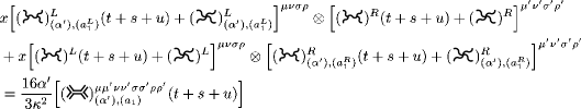
Figure 3: The diagrammatical expression for the generalized mapping of the 4-point gravity amplitude as a product of Yang-Mills amplitudes at order $\alpha^{\prime}$.

This relation is essentially equivalent to the 3-vertex relation at order $\alpha^{\prime}$. The 4-point relation at order $\alpha^{\prime}$ rules out the possibility of a $P_{1}$ term in the generalized mapping. The full KLT relation at order $\alpha^{\prime 2}$ is:

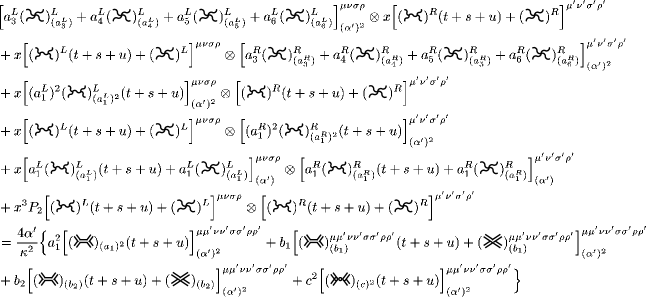
Figure 4: The diagrammatical expression for the generalized mapping of the 4-point gravity amplitude into the product of Yang-Mills amplitudes at order $\alpha^{\prime 2}$.

The coefficients in the above expression need to be taken in agreement with the generalized KLT solution in order for this identity to hold. A profound consequence of the KLT relations is that they link the sum of a certain class of diagrams in Yang-Mills theory with a corresponding sum of diagrams in gravity, for very specific values of the constants in the Lagrangian. At glance we do not observe anything manifestly about the decomposition of e.g., vertex rules, – however this should be investigated more carefully before any conclusions can be drawn. The coefficient equations cannot directly be transformed into relations between diagrams, – this can be seen by calculation. However reinstating the solution for the coefficients it is possible to turn the above equation for the 4-amplitude at order $\alpha^{\prime 2}$ into interesting statements about diagrams. Relating all $P_{2}$ terms gives e.g., the following remarkable diagrammatic statement:

Figure 5: A diagrammatic relationship on the Yang-Mill side for the tree operators in the effective action between operators of unit order and order $\alpha^{\prime 2}$.

The surprising fact is that from the relations which apparently link gravity and Yang-Mills theory only, one can eliminate the gravity part to obtain relations entirely in pure Yang-Mills theory.

Similarly, relating all contributions with $a_{1}^{2}$ gives:

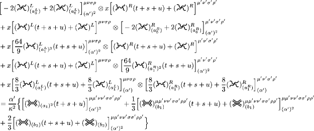
Figure 6: The essential diagrammatic relationship between gauge and gravity diagrams.

furthermore we have a relationship generated by the $ca_{1}$ parts:

Figure 7: Another diagrammatic relationship on the Yang-Mills side between order $\alpha^{\prime 2}$ and $\alpha^{\prime}$ operators.

These diagrammatical relationships can be readily checked by explicit calculation. It is quite remarkable that the KLT relations provide such detailed statements about pure Yang-Mills effective field theories, without any reference to gravity at all. To explain the notation in the above diagrammatic statements. An uppercase $L$ or $R$ states that the scattering amplitude originates from a left or a right mover respectively. The lower indices e.g. $(\alpha^{\prime})$ and the coupling constants e.g. $(a_{3}^{L})$ or $(a_{1}^{L})^{2}$ denote respectively the order of $\alpha^{\prime}$ in the particular amplitude and the coupling constant prefactor obtained when this particular part of the amplitude is generated from the generic Lagrangian. The parentheses with $(t+s+u)$ denote that we are supposed to sum over all $t$, $s$ and $u$ channels for this particular amplitude.

V Discussion

It has been observed that it is possible to generalize the KLT open/closed string relations in the effective field theory framework. The KLT relations are seen to serve as mapping relations between the tree effective field theories for Yang-Mills and gravity. The belief that general relativity is in fact an effective field theory at loop orders, makes investigations of its tree level manifestations and connections to other effective actions interesting. Links such as KLT, which are applicable and very simplifying in actual calculations should be exploited and investigated at the effective Lagrangian level. An important result of our investigations is the generalization of the KLT relations. It is found that one cannot completely replace the sine function in the KLT relations by an arbitrary function. To order $O(\alpha^{\prime 3})$ it is possible to replace the sine with an odd third order polynomial in $x$. However, the degree of freedom represented by $P_{2}$ can be completely absorbed into a rescaling of $\alpha^{\prime}$ at this order, so additional investigations are required before any conclusions can be drawn. The mapping relations between the effective theories are found to be broader than those given completely from the KLT relations as the coefficient $P_{2}$ in the generalized framework can be chosen freely. Such a rescaling of $P_{2}$ represents an additional freedom in the mapping. It has been shown that despite this generalization, the effective extension of the KLT relations is still rather restrictive.

The possibility of an antisymmetric coupling of gravitons needed in the effective action of a heterotic string has also been allowed for and is seen to be consistent with the original and generalized KLT relations. We have learned that detailed diagrammatic statements can be deduced from the KLT relations. This presents very interesting aspects which perhaps can be used to gain additional insight in issues concerning effective Lagrangian operators. Furthermore we expect this process to continue, – at order $O(\alpha^{\prime 4})$ we assume that the KLT relations will tell us about new profound diagrammatic relationships between effective field theory on-shell operators in gauge theory and gravity.

The generalized mapping relations represent an effective field theory version of the well known KLT relations. We have used what we knew already from string theory about the KLT relations to produce a more general description of mapping relations between gravity and Yang-Mills theory. String theory is not really needed in the effective field theory setting. All that is used here is the tree scattering amplitudes. Exploring if or if not a mapping from the general relativity side to the gauge theory side is possible produces the generalized KLT relations. The KLT relations could also be considered in the case of external matter. In this case, operators as the Ricci tensor and the scalar curvature will not vanish on-shell. Such an approach could perhaps explain more about the KLT relations and introduce additional aspects in the mapping of operators.

KLT relations involving loops are not yet resolved. One can preform some calculations by making cuts of the diagrams using the unitarity of the S-matrix but no direct factorizations of loop scattering amplitudes have been seen to support a true loop extension of the KLT relations. Progress in this direction still waits to be seen, and perhaps such loop extensions are not possible. Loops in string theory and in field theory are not directly comparable, and complicated issues with additional string theory modes in the loops seem to be unavoidable in extensions of the KLT relations beyond tree level. Perhaps since 4-point scattering amplitudes are much less complicated compared to 5-point amplitudes, it would be actually more important first to check the mapping solutions at the 5-point level before considering the issue of loop amplitudes.

- (1) N. E. J. Bjerrum-Bohr, Phys. Lett. B 560, 98 (2003) [arXiv:hep-th/0302131].
- (2) H. Kawai, D. C. Lewellen and S. H. Tye, Nucl. Phys. B 269 (1986) 1.
- (3) A. A. Tseytlin, Nucl. Phys. B 276 (1986) 391 [Erratum-ibid. B 291 (1987) 876].
- (4) R. R. Metsaev and A. A. Tseytlin, Phys. Lett. B 185 (1987) 52.
- (5) A. A. Tseytlin, JETP Lett. 43 (1986) 263 [Pisma Zh. Eksp. Teor. Fiz. 43 (1986) 209].
- (6) D. J. Gross and E. Witten, Nucl. Phys. B 277, 1 (1986).
- (7) C. G. Callan, I. R. Klebanov and M. J. Perry, Nucl. Phys. B 278 (1986) 78; C. G. Callan, E. J. Martinec, M. J. Perry and D. Friedan, Nucl. Phys. B 262, 593 (1985); C. G. Callan, C. Lovelace, C. R. Nappi and S. A. Yost, Nucl. Phys. B 288 (1987) 525.
- (8) D. J. Gross, J. A. Harvey, E. J. Martinec and R. Rohm, Nucl. Phys. B 256 (1985) 253; D. J. Gross, J. A. Harvey, E. J. Martinec and R. Rohm, Nucl. Phys. B 256 (1985) 253; D. J. Gross and J. H. Sloan, Nucl. Phys. B 291 (1987) 41.
- (9) C. M. Hull and P. K. Townsend, Nucl. Phys. B 301 (1988) 197.
- (10) S. Sannan, Phys. Rev. D 34, 1749 (1986).
- (11) F. A. Berends, W. T. Giele and H. Kuijf, Phys. Lett. B 211 (1988) 91.
- (12) Z. Bern, L. J. Dixon, D. C. Dunbar, M. Perelstein and J. S. Rozowsky, Nucl. Phys. B 530 (1998) 401 [arXiv:hep-th/9802162].
- (13) Z. Bern, L. J. Dixon, M. Perelstein and J. S. Rozowsky, Phys. Lett. B 444 (1998) 273 [arXiv:hep-th/9809160]; Z. Bern, L. J. Dixon, M. Perelstein and J. S. Rozowsky, Nucl. Phys. B 546 (1999) 423 [arXiv:hep-th/9811140].
- (14) Z. Bern, Living Rev. Rel. 5 (2002) 5 [arXiv:gr-qc/0206071].
- (15) Z. Bern, L. J. Dixon and D. A. Kosower, Ann. Rev. Nucl. Part. Sci. 46 (1996) 109 [arXiv:hep-ph/9602280].
- (16) Z. Bern, D. C. Dunbar and T. Shimada, Phys. Lett. B 312 (1993) 277 [arXiv:hep-th/9307001].
- (17) D. C. Dunbar and P. S. Norridge, Nucl. Phys. B 433 (1995) 181 [arXiv:hep-th/9408014].
- (18) Z. Bern, A. De Freitas and H. L. Wong, Phys. Rev. Lett. 84 (2000) 3531 [arXiv:hep-th/9912033].
- (19) Z. Bern and A. K. Grant, Phys. Lett. B 457 (1999) 23 [arXiv:hep-th/9904026].
- (20) W. Siegel, Phys. Rev. D 47 (1993) 5453 [arXiv:hep-th/9302036]; in Proceedings of Strings 1993, eds. M. B. Halpern, A. Sevrin and G. Rivlis (World Scientific, Singapore, 1994) [arXiv:hep-th/9308133].
- (21) G. ’t Hooft and M. J. Veltman, Annales Poincare Phys. Theor. A 20 (1974) 69.
- (22) M. H. Goroff and A. Sagnotti, Nucl. Phys. B 266 (1986) 709; A. E. van de Ven, Nucl. Phys. B 378 (1992) 309.
- (23) S. Deser and P. van Nieuwenhuizen, Phys. Rev. D 10 (1974) 401; S. Deser and P. van Nieuwenhuizen, Phys. Rev. D 10 (1974) 411; S. Deser, H. S. Tsao and P. van Nieuwenhuizen, Phys. Rev. D 10 (1974) 3337.
- (24) S. Weinberg, PhysicaA 96 (1979) 327.
- (25) K. S. Stelle, Gen. Rel. Grav. 9 (1978) 353.
- (26) J. Z. Simon, Phys. Rev. D 41 (1990) 3720.
- (27) J. F. Donoghue, Phys. Rev. D 50 (1994) 3874 [arXiv:gr-qc/9405057].
- (28) N. E. J. Bjerrum-Bohr, J. F. Donoghue and B. R. Holstein, submitted to Phys. Rev. D, [arXiv:hep-th/0211071].
- (29) N. E. J. Bjerrum-Bohr, J. F. Donoghue and B. R. Holstein, Phys. Rev. D 67, 084033 (2003) [arXiv:hep-th/0211072].
- (30) J. F. Donoghue, B. R. Holstein, B. Garbrecht and T. Konstandin, Phys. Lett. B 529, 132 (2002) [arXiv:hep-th/0112237].
- (31) N. E. J. Bjerrum-Bohr, Phys. Rev. D 66 (2002) 084023 [arXiv:hep-th/0206236].
- (32) S. Deser and A.N. Redlich, Phys. Lett. 176B (1986), 350.
- (33) D. C. Dunbar and N. W. Turner, Phys. Lett. B 547 (2002) 278 [arXiv:hep-th/0203104].
- (34) Z. Bern and T. Shimada, Phys. Lett. B 197 (1987) 119.
- (35) D. Hochberg and T. Shimada, Progr. of Theor. Phys., Vol. 78, No. 3, 1987 (680).
- (36) M. B. Green, J. H. Schwarz and E. Witten, Superstring theory (Cambridge University Press, 1987)
- (37) P. van Nieuwenhuizen and C. C. Wu, J. Math. Phys. 18 (1977) 182.
- (38) M. T. Grisaru, H. N. Pendleton and P. van Nieuwenhuizen, Phys. Rev. D 15 (1977) 996.
- (39) M. T. Grisaru and H. N. Pendleton, Nucl. Phys. B 124 (1977) 81.
- (40) M. T. Grisaru, Phys. Lett. B 66 (1977) 75.