Thermodynamics of the ${\cal N}=2^{*}$ flow

MCTP-03-25 hep-th/0305064

May 2003

1 Introduction

Over the last few years, gauge theory/string theory duality [1] (see [2] for a review) has proven to be a very useful tool to address nonperturbative questions in gauge theories. Essentially, this duality states that, say, four dimensional gauge theories at large ’t Hooft coupling, $g_{YM}^{2}N\gg 1$, can be described by dual string theories in weakly curved supergravity backgrounds. In the large $N$ but fixed ’t Hooft coupling limit, the string coupling vanishes, and one can consistently restrict the string theory side of the correspondence to the massless sector of type IIB supergravity. Thus the computations on the supergravity side shed light on the nonperturbative gauge theory dynamics. On the other hand, nonperturbative effects in the gauge theory potentially could tell us something new about the dual supergravity. This is indeed the case with finite temperature phase transitions in gauge theories [3, 4, 5, 6, 7]. Specifically, in [3], it was demonstrated how the (kinematic) confinement-deconfinement phase transition of ${\cal N}=4$, $SU(N)$ supersymmetric Yang-Mills theory on ${\mathbb{R}}\times S^{3}$ was mapped by the duality correspondence to the previously discovered Hawking-Page phase transition in an anti-de Sitter background [8].

With a field theory intuition in mind, a new prediction for the higher dimensional black holes (and a phase transition in an infinite volume) was obtained in [4]. Namely, using the fact that the chirally symmetric phase of the Klebanov-Strassler (KS) cascading gauge theories [9, 10] exists only above a certain critical temperature, it was proposed in [4] that the dual supergravity backgrounds also would have a regular Schwarzschild horizon only above certain horizon temperatures. While there is a good understanding of the high temperature thermodynamics of the system (in a chirally symmetric phase) [5], the low temperature phase (and the phase transition) requires substantial numerical work and is not yet understood. Thus, strictly speaking, the prediction for the new type of black holes of [4] has not yet been verified in the KS model. Nevertheless, black holes that exhibit a phase transition predicted in [4] were shown to exist [6, 7] in a different (but closely related) model — the supergravity dual to pure ${\cal N}=1$, $SU(N)$ SYM theory [11]. Unfortunately, the latter black holes were shown to be thermodynamically unstable [12, 7], and thus it is not clear whether the phase transition, while mathematically allowed, is actually physically occurring.

In this paper we discuss yet another system which we argue undergoes a finite temperature phase transition, namely the ${\cal N}=2^{*}$ theory, or in other words ${\cal N}=4$, $SU(N)$ SYM softly broken by a hypermultiplet mass term to ${\cal N}=2$ gauge theory. The supergravity dual to this gauge theory was constructed by Pilch and Warner (PW) in [13], and the precise duality map between the gauge theory and the supergravity was explained in [14, 15]. Here we consider the ${\cal N}=2^{*}$ gauge theory at finite temperature, realized as a non extremal deformation of the PW flow. The argument for the existence of a phase transition in this system is quite simple. For the high temperature phase, the mass deformation is irrelevant and we expect the standard near-extremal D3 brane thermodynamics. In this phase (which we refer to as the “black hole phase”, $BH$) all the thermodynamics quantities scale as $N^{2}$; for example, the entropy goes as $S_{BH}\propto N^{2}VT^{3}$. On the other hand, the low temperature phase is rather different. Imagine first completely turning off the temperature. In this case the ${\cal N}=2^{*}$ gauge theory is exactly soluble [16]. Its low energy effective description (valid well below the hypermultiplet mass scale) is given in terms of ${\cal N}=2$, $U(1)^{N-1}$ gauge theory. This gauge theory has on the order of $N$ free degrees of freedom. We expect that this low energy effective description is still valid for temperatures much lower than the hypermultiplet mass. Thus in the low temperature phase (which we denote the “finite temperature Coulomb phase” or the Pilch-Warner phase, $PW$) the thermodynamic quantities of the ${\cal N}=2^{*}$ gauge theory would scale as the first power of $N$, so that, e.g., for the entropy, $S_{PW}\propto NVT^{3}$. This $N^{2}$ versus $N$ scaling of degrees of freedom suggests the presence of a phase transition between the $BH$ and $PW$ phases, each of which in principle exists at all temperatures.

The physical picture we have in mind for the phase transition is as follows. Start with a high temperature $BH$ phase. In this phase the free energy will start negative at very high temperatures (as for the black D3 branes), and would gradually increase as the temperature is lowered. We expect that at some $T=T_{c}$ the free energy would become zero, $F_{BH}(T_{c})=0$, and for $T<T_{c}$ it would become positive. In the large $N$ limit, the free energy of the $PW$ phase is down by ${\cal O}(1/N)$, and may be taken to be zero. Thus the $PW$ phase should be thermodynamically favorable for low temperatures, $T<T_{c}$. We expect that both the $PW$ and the $BH$ phases are thermodynamically stable. Moreover, there should be a well defined high temperature expansion of the $BH$ phase.

In the next section we summarize our results. In section 3 we recall the salient features of the ${\cal N}=2^{*}$ gauge theory, and discuss the expectation for its finite temperature deformation. We then review the PW ${\cal N}=2^{*}$ renormalization group (RG) flow in five dimensions and discuss its non-extremal deformation. The exact ten dimensional lift of the “temperature deformed” five dimensional PW flow is constructed in section 4. In section 5 we analytically determine the leading in $m/T$ correction to the near-extremal D3 brane geometry induced by the ${\cal N}=2$ hypermultiplet mass $m$. Finally, in section 6 we discuss the thermodynamics and the signature of the phase transition. First, we explain the computation of the free energy and the energy (mass) of the deformed supergravity backgrounds, and compute the difference of the free energies of the $BH$ and the $PW$ phases. This computation is valid for arbitrary values of $m/T$, and thus can be used to study the phase transition. Then, using the results of section 5, we compute the leading correction (in the high temperature phase) to the black D3 brane thermodynamics. We find that the first law of thermodynamics applied to the high temperature phase is violated. We speculate on the relevance of the (induced) chemical potential for the resolution of this paradox. We end with some comments on the numerical verification of the phase transition.

Before proceeding, we would like to comment on the study of the thermodynamics of the closely related ${\cal N}=1^{*}$, $SU(N)$ gauge theory [18]. As its name suggests, the ${\cal N}=1^{*}$ gauge theory is ${\cal N}=4$, $SU(N)$ SYM softly broken by a chiral multiplet mass term to ${\cal N}=1$. Unlike the ${\cal N}=2^{*}$ theory, however, the dual supergravity background to this model [19] (PS) is known only in the probe approximation. The study of thermodynamics in [18] was also done in the probe approximation. Only the entropy was computed in the high temperature regime of the non-extremal PS background; while the free energy and the energy were not computed independently, they were obtained by enforcing the first law of thermodynamics. As we will see from the thermodynamics of the ${\cal N}=2^{*}$ model discussed here, the computation of the entropy alone does not allow us to reproduce the free energy — it appears one needs to compute the induced chemical potential as well. It would be of interest to repeat the ${\cal N}=2^{*}$ analysis presented here to the ${\cal N}=1^{*}$ model. But first, the exact extremal geometry of the ${\cal N}=1^{*}$ theory has to be understood.

2 Summary of results and outlook

As the bulk of the paper is rather technical, we highlight our main results in this section.
   We first observe that the five dimensional gauged supergravity flow of ${\cal N}=2^{*}$ PW [13] can be deformed to yield a non-extremal black hole geometry with regular horizon. The consistency of the $D=5$, ${\cal N}=8$ gauged supergravity truncation then implies that this black hole solution can be uplifted to the full ten dimensional solution of type IIB supergravity. We explicitly verify that this is indeed so. This non-extremal deformation is interpreted as the supergravity dual to the finite temperature ${\cal N}=2^{*}$ $SU(N)$ gauge theory in the deconfined phase, which we refer to as the $BH$ phase.
   We show that there is a three parameter family of five dimensional black holes admitting regular horizons. These three parameters are the temperature $T$ and the (generically different) masses of the bosonic $m_{b}$ and fermionic $m_{f}$ components of the ${\cal N}=2$ hypermultiplet. All regular horizon non-extremal solutions asymptote to $AdS_{5}$, which is consistent with the gauge theory expectation that both the temperature and the mass deformations should be irrelevant in the ultraviolet of the gauge theory. Asymptotic ${\cal N}=2$ supersymmetry of the extremal PW geometry imposes a constraint on the leading nontrivial asymptotics of the two five dimensional supergravity scalars in the non-extremal deformation. The latter reduces the number of independent parameters of the regular horizon solution to two: one related to the temperature, and the other to the ${\cal N}=2$ hypermultiplet mass $m=m_{b}=m_{f}$.
   In the high temperature limit, $\alpha_{1}\equiv(m_{b}/T)^{2}\ll 1$, $\alpha_{2}\equiv m_{f}/T\ll 1$, the five dimensional black hole solution is a small deformation of the finite temperature $AdS_{5}$ geometry, representing the $S^{5}$ reduction of the throat region of the near extremal D3 branes. We analytically determine the leading correction in $\alpha_{i}$ of the near extremal $AdS_{5}$ geometry. As expected from gauge theory arguments, asymptotic ${\cal N}=2$ supersymmetry sets $\alpha_{1}\sim(\alpha_{2})^{2}$.
   After constructing the black hole solution, we turn to the study of thermodynamics. We discuss the computation of the free energy $F$, the entropy $S$, and the energy $E$ of the non-extremal deformation of the PW flow. The entropy is just the Bekenstein-Hawking entropy of the horizon, and is determined from the infrared data of the geometry. The free energy, or more precisely $FT$, is the Euclidean gravitational action, and the energy $E$ is the conserved ADM mass of the geometry. Note that computing both $E$ and $F$ requires the knowledge of the IR and the UV data of the solution. Furthermore, we verify that $F=E-TS$ is identically satisfied in the supergravity.
   While the computation of the entropy is straightforward, both the free energy and the energy diverges, and requires regularization. Following [20], we compute $F$ and $E$ with respect to a reference geometry which we take to be the supersymmetric PW flow with periodically identified (Euclidean) time direction with periodicity equal to the inverse horizon temperature. We call this geometry the “$PW$ phase”. The prescription of [20] requires the introduction of a boundary cutoff and the matching of induced geometries (and matter fields) for the background at hand and the reference one “up to sufficiently high order” [20]. We apply the “minimal subtraction” prescription for matching, where only the leading asymptotics of the induced geometries and the matter fields are matched. This prescription gives the correct answers for simple black hole geometries such as the Schwarzschild-anti-de Sitter solution. It also works in more complicated cases such as the nonabelian black hole solutions of [7].
   Using this minimal subtraction prescription for the free energy and the energy, we find an explicit analytical expression for $F_{BH}-F_{PW}$ (or $E_{BH}-E_{PW}$) is terms of the coefficients of the subleading ultraviolet asymptotics of the five dimensional scalars inducing the Pilch-Warner flow [13]. An added bonus of using the PW background (with appropriately compactified Euclidean time direction) as the reference one in $F$ and $E$ regularization is the fact that the purported phase transition between the high temperature $BH$ phase and the low temperature $PW$ phase arises when $\Delta^{BH}_{PW}\equiv F_{BH}-F_{PW}$ changes sign.
   Using the high temperature expansion (corresponding to deformations from the non-extremal $AdS_{5}$ geometry), and working to leading order in $m/T$, we analytically compute the corresponding deformations of the thermodynamic quantities. While $F=E-TS$ continues to be satisfied after regulation, we however find that $TdS\neq dE$. We have verified our prediction for the leading correction to the free energy numerically. This indirectly confirms the violation of the first law of thermodynamics.
   Though we have been unable to find a satisfactory explanation for this apparent contradiction with the first law of thermodynamics for the high temperature phase of the ${\cal N}=2^{*}$ flow, we point out that this paradox could be resolved once we include a certain chemical potential induced by the fermionic mass term of the ${\cal N}=2$ hypermultiplet.

Perhaps the most intriguing conclusion we have reached is the fact that the proper interpretation of a finite temperature deformation of the Pilch-Warner geometry appears to require the introduction of a nonvanishing chemical potential dual to the sources that are turned on in the UV. This induced chemical potential follows from the conjecture that the string theory partition function in the gauge/string theory correspondence is dual to the gauge theory grand canonical partition function. In section 6.3 we outline the general arguments leading to such a statement. It would be interesting to verify this in a more general setting, e.g., by studying the finite temperature deformations of generic holographic renormalization group flows as in [21, 22].

The original motivation for the study of the ${\cal N}=2^{*}$ thermodynamics presented here was to study and confirm the phase transition between the $BH$ and the $PW$ phases. However, our analysis for this question is as yet inconclusive. While the high temperature expansion is suggestive that such a phase transition occurs, additional analytical or numerical work is required to extrapolate to the region $m\sim T$ where solid evidence of the transition would be obtained. We hope to report on these results in a separate publication. Finally, it is interesting to understand the “hydrodynamic description” of the $BH$ phase of the ${\cal N}=2^{*}$ gauge theory along the lines of [23].

3 ${\cal N}=2^{*}$ RG flow and its non-extremal deformation in five dimensions

3.1 The gauge theory picture

In the language of four-dimensional ${\cal N}=1$ supersymmetry, the mass deformed ${\cal N}=4$ $SU(N)$ Yang-Mills theory (${\cal N}=2^{*}$) in ${\mathbb{R}}^{3,1}$ consists of a vector multiplet $V$, an adjoint chiral superfield $\Phi$ related by ${\cal N}=2$ supersymmetry to the gauge field, and two additional adjoint chiral multiplets $Q$ and $\tilde{Q}$ which form an ${\cal N}=2$ hypermultiplet. In addition to the usual gauge-invariant kinetic terms for these fields, the theory has additional interactions and a hypermultiplet mass term given by the superpotential

$$W=\frac{2\sqrt{2}}{g_{YM}^{2}}\mathop{\rm Tr}([Q,\tilde{Q}]\Phi)+\frac{m}{g_{YM}^{2}}(\mathop{\rm Tr}Q^{2}+\mathop{\rm Tr}\tilde{Q}^{2})\,.$$ (3.1)

When $m=0$ the gauge theory is superconformal with $g_{YM}$ characterizing an exactly marginal deformation. The theory has a classical $3(N-1)$ complex dimensional moduli space, which is protected by supersymmetry against (non)-perturbative quantum corrections.

When $m\neq 0$, the ${\cal N}=4$ supersymmetry is softly broken to ${\cal N}=2$. This mass deformation lifts the $\{Q,\ \tilde{Q}\}$ hypermultiplet moduli directions, leaving the $(N-1)$ complex dimensional Coulomb branch of the ${\cal N}=2$, $SU(N)$ Yang-Mills theory, parameterized by expectation values of the adjoint scalar

$$\Phi={\rm diag}(a_{1},a_{2},\cdots,a_{N})\,,\quad\sum_{i}a_{i}=0\,,$$ (3.2)

in the Cartan subalgebra of the gauge group. For generic values of the moduli $a_{i}$, the gauge symmetry is broken to that of the Cartan subalgebra $U(1)^{N-1}$, up to the permutation of individual $U(1)$ factors. Additionally, the superpotential (3.1) induces the RG flow of the gauge coupling. While from the gauge theory perspective it is straightforward to study this ${\cal N}=2^{*}$ theory at any point on the Coulomb branch [16], the PW supergravity flow [13] corresponds to a particular Coulomb branch vacuum. More specifically, matching the probe computation in gauge theory and the dual PW supergravity flow, it was argued in [14] that the appropriate Coulomb branch vacuum corresponds to a linear distribution of the vevs (3.2) as

$$a_{i}\in[-a_{0},a_{0}],\qquad a_{0}^{2}=\frac{m^{2}g_{YM}^{2}N}{\pi}\,,$$ (3.3)

with (continuous in the large $N$ limit) linear number density

$$\rho(a)=\frac{2}{m^{2}g_{YM}^{2}}\sqrt{a_{0}^{2}-a^{2}},\qquad\int_{-a_{0}}^{a_{0}}da\,\rho(a)=N\,.$$ (3.4)

Unfortunately, the extension of the $N=2^{*}$ gauge/gravity correspondence of [13, 14, 15] for vacua other than (3.4) is not known.

In [14, 15] the dynamics of the gauge theory on the D3 brane probe in the PW background was studied in detail. It was shown in [14] that the probe has a one complex dimensional moduli space, with bulk induced metric precisely equal to the metric on the appropriate one complex dimensional submanifold of the ${\cal N}=2^{*}$, $SU(N+1)$ Donagi-Witten theory Coulomb branch. This one dimensional submanifold is parameterized by the expectation value $u$ of the $U(1)$ complex scalar on the Coulomb branch of the theory where $SU(N+1)\rightarrow U(1)\times SU(N)_{PW}$. Here the _PW subscript denotes that the $SU(N)$ factor is in the Pilch-Warner vacuum (3.4). Whenever $u$ coincides with any of the $a_{i}$ of the PW vacuum, the moduli space metric diverges, signaling the appearance of additional massless states. An identical divergence is observed [14, 15] for the probe D3-brane at the enhançon singularity of the PW background. Away from the singularity locus, $u=a\in[-a_{0},a_{0}]$, the gauge theory computation of the probe moduli space metric is 1-loop exact. This is due to the suppression of instanton corrections in the large $N$ limit [14, 24] of ${\cal N}=2$ gauge theories.

Consider now ${\cal N}=2^{*}$ gauge theory at finite temperature $T$. Turning on a mass $m$ for the hypermultiplet sets a strong coupling scale $\Lambda\propto m$. We expect to find two different phases of this gauge theory, depending on whether $T\gg\Lambda$ or $T\ll\Lambda$. In the former case the effect of the mass deformation is negligible, and we expect to recover the ${\cal N}=4$ thermodynamics. In particular, conformal invariance dictates that the free energy scales like $T^{4}$, with a prefactor of $N^{2}$ indicative of the scaling of the number of degrees of freedom. At weak ’t Hooft coupling the familiar result reads [25]

$$F_{SYM}=-\frac{\pi^{2}}{6}N^{2}VT^{4}.$$ (3.5)

By symmetry arguments, we expect the corrections to the free energy (3.5) due to the mass deformation (3.1) to be of order ${\cal O}\left(m^{2}/T^{2}\right)$. The $N^{2}$ scaling of the thermodynamic quantities naturally occurs in the ten-dimensional black holes describing the non-extremal deformation of the dual supergravity backgrounds. For this reason we will call the high temperature phase of ${\cal N}=2^{*}$ SYM the $BH$ or black hole phase.

In the other limit, we expect qualitatively different physics in the low temperature phase of ${\cal N}=2^{*}$ SYM. Ignoring $T$ in the first approximation, the low energy effective description of the ${\cal N}=2^{*}$ theory is given by free $U(1)^{N-1}$ SYM as explained above. This effective description breaks down at scales of order the strong coupling scale, i.e. $m$, but is appropriate as we turn on the temperature provided $T\ll m$. The number of (free) degrees of freedom of this effective low energy description scales like $N$, which must be reflected in the scaling of the thermodynamics quantities such as the entropy, $S\propto NVT^{3}$. We denote this phase the “finite temperature Coulomb phase”, or the $PW$ phase. Notice that

$$\frac{F_{PW}}{F_{BH}}\sim\frac{1}{N},$$ (3.6)

and thus vanishes in the large-$N$ limit. Qualitatively, we expect the free energy of the ${\cal N}=2^{*}$ SYM to behave as in Fig. 1.

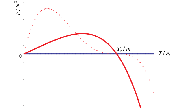
Figure 1: The expected behavior of free energies of the $BH$ (red curves) and the $PW$ (blue curve) phases ($F_{BH}$ and $F_{PW}$) as a function of $T/m$ in the large $N$ limit. The dotted line for the $BH$ phase would imply a second order phase transition, while the solid line would imply a first order phase transition.

Given two possible phases, $BH$ and $PW$, the most favorable one is that with lowest free energy. Thus the signature of a phase transition in the ${\cal N}=2^{*}$ theory would be a change in sign in the difference $\Delta^{BH}_{PW}\equiv F_{BH}-F_{PW}$. This suggests that, in order to have a phase transition, the sign of the $O(m^{2}/T^{2})$ correction to (3.5) must be positive so that, when the temperature is lowered from an initial high temperature phase, $F_{BH}$ will be driven above $F_{PW}$ at a finite temperature $T_{c}$. While we have not performed this computation perturbatively in the ’t Hooft coupling, we have instead analytically determined the ${\cal O}(m^{2}/T^{2})$ correction for strong ’t Hooft coupling in the dual supergravity computation. We find that this correction indeed has a positive coefficient (6.48) at strong ’t Hooft coupling. This provides evidence for a phase transition, although further investigation is necessary beyond leading order to substantiate this claim.

3.2 The PW renormalization group flow

The gauge theory RG flow induced by the superpotential (3.1) corresponds to a five dimensional gauged supergravity flow induced by a pair of scalars, $\alpha\equiv\sqrt{3}\ln\rho$ and $\chi$. The effective five-dimensional action is

$$S=\frac{1}{4\pi G_{5}}\,\int_{{\cal M}_{5}}d\xi^{5}\sqrt{-g}\left({\textstyle{\frac{1}{4}}}R-(\partial\alpha)^{2}-(\partial\chi)^{2}-{\cal P}\right)\,,$$ (3.7)

where the potential ${\cal P}$ is

$${\cal P}=\frac{1}{16}\left[\left(\frac{\partial W}{\partial\alpha}\right)^{2}+\left(\frac{\partial W}{\partial\chi}\right)^{2}\right]-\frac{1}{3}W^{2}\,,$$ (3.8)

with the superpotential

$$W=-\frac{1}{\rho^{2}}-\frac{1}{2}\rho^{4}\cosh(2\chi)\,.$$ (3.9)

Note that we have chosen identical normalizations for $\alpha$ and $\chi$ to highlight the general $D=5$, ${\cal N}=2$ features of the flow. The PW geometry [13] has the flow metric

$$ds_{5}^{2}=e^{2A}\left(-dt^{2}+d\vec{x}\,^{2}\right)+dr^{2}\,.$$ (3.10)

Solving the Killing spinor equations for a supersymmetric flow then yields the first order equations

$$\frac{dA}{dr}=-\frac{1}{3}W\,,\qquad\frac{d\alpha}{dr}=\frac{1}{4}\frac{\partial W}{\partial\alpha}\,,\qquad\frac{d\chi}{dr}=\frac{1}{4}\frac{\partial W}{\partial\chi}\,.$$ (3.11)

It is straightforward to verify that solutions to these flow equations will automatically satisfy the scalar and Einstein equations of motion.

3.2.1 Asymptotics of the PW flow

This system was solved in [13] by rewriting the equations in terms of $\chi$ as an independent variable. Given this explicit solution of the flow equations, it is easy to extract the UV/IR asymptotics. In the ultraviolet, $r\to+\infty$, we find

$${\rm UV:}\qquad\qquad\rho\to 1_{-},\qquad\chi\to 0_{+},\qquad A\to\frac{1}{2}\ r\,.$$ (3.12)

This corresponds to the scalars approaching the maximally symmetric $AdS_{5}\times S^{5}$ UV fixed point of the potential ${\cal P}$. In the infrared, $r\to 0$, we find instead

$${\rm IR:}\qquad\qquad\rho\to 0_{+},\qquad\chi\to+\infty,\qquad A\to-\frac{8}{3}\chi\,.$$ (3.13)

As will be apparent later, this flow to the IR will be cut off at finite temperature.

3.3 The non-extremal PW flow

We now consider deforming the PW flow by turning on non-extremality in the metric. Since the deformed flow breaks supersymmetry, we can no longer appeal to first order equations, but must consider the second order equations of motion. The action (3.7) yields the Einstein equation

$${\frac{1}{4}}R_{\mu\nu}=\partial_{\mu}\alpha\partial_{\nu}\alpha+\partial_{\mu}\chi\partial_{\nu}\chi+{\frac{1}{3}}g_{\mu\nu}{\cal P}\,,$$ (3.14)

and the scalar equations

$$\mathop{\mathchoice{{\vbox{\vbox{\hrule height=0.32pt\hbox{\vrule width=0.32pt,height=8.0pt\kern 8.0pt\vrule width=0.32pt}\hrule height=0.32pt}}}}{{\vbox{\vbox{\hrule height=0.32pt\hbox{\vrule width=0.32pt,height=8.0pt\kern 8.0pt\vrule width=0.32pt}\hrule height=0.32pt}}}}{{\vbox{\vbox{\hrule height=0.9pt\hbox{\vrule width=0.9pt,height=6.3pt\kern 6.3pt\vrule width=0.9pt}\hrule height=0.9pt}}}}{{\vbox{\vbox{\hrule height=0.9pt\hbox{\vrule width=0.9pt,height=4.5pt\kern 4.5pt\vrule width=0.9pt}\hrule height=0.9pt}}}}}\alpha={\frac{1}{2}}{\frac{\partial{\cal P}}{\partial\alpha}}\,,\qquad\mathop{\mathchoice{{\vbox{\vbox{\hrule height=0.32pt\hbox{\vrule width=0.32pt,height=8.0pt\kern 8.0pt\vrule width=0.32pt}\hrule height=0.32pt}}}}{{\vbox{\vbox{\hrule height=0.32pt\hbox{\vrule width=0.32pt,height=8.0pt\kern 8.0pt\vrule width=0.32pt}\hrule height=0.32pt}}}}{{\vbox{\vbox{\hrule height=0.9pt\hbox{\vrule width=0.9pt,height=6.3pt\kern 6.3pt\vrule width=0.9pt}\hrule height=0.9pt}}}}{{\vbox{\vbox{\hrule height=0.9pt\hbox{\vrule width=0.9pt,height=4.5pt\kern 4.5pt\vrule width=0.9pt}\hrule height=0.9pt}}}}}\chi={\frac{1}{2}}{\frac{\partial{\cal P}}{\partial\chi}}\,.$$ (3.15)

For a finite temperature deformation of the flow metric (3.10), we take

$$ds_{5}^{2}=e^{2A}\left(-e^{2B}\ dt^{2}+d\vec{x}\,^{2}\right)+dr^{2}\,,\\$$ (3.16)

where $e^{2B}$ represents a blackening function. Note that we choose to retain $g_{rr}=1$ since any non-trivial factor can be absorbed into a redefinition of $r$.

Substituting this metric ansatz into the equations of motion, (3.14) and (3.15), we find

$$\begin{split}0&=\alpha^{\prime\prime}+\left(4A^{\prime}+B^{\prime}\right)\alpha^{\prime}-\frac{1}{2}\frac{\partial{\cal P}}{\partial\alpha}\,,\\ 0&=\chi^{\prime\prime}+\left(4A^{\prime}+B^{\prime}\right)\chi^{\prime}-\frac{1}{2}\frac{\partial{\cal P}}{\partial\chi}\,,\\ 0&=B^{\prime\prime}+\left(4A^{\prime}+B^{\prime}\right)B^{\prime}\,,\\ &\frac{1}{4}A^{\prime\prime}+\frac{1}{4}B^{\prime\prime}+\left(A^{\prime}\right)^{2}+\frac{1}{4}\left(B^{\prime}\right)^{2}+\frac{5}{4}A^{\prime}B^{\prime}=-\frac{1}{3}{\cal P}\,,\\ &-A^{\prime\prime}-\frac{1}{4}B^{\prime\prime}-\left(A^{\prime}\right)^{2}-\frac{1}{4}\left(B^{\prime}\right)^{2}-\frac{1}{2}A^{\prime}B^{\prime}=\left(\alpha^{\prime}\right)^{2}+\left(\chi^{\prime}\right)^{2}+\frac{1}{3}{\cal P}\,.\end{split}$$ (3.17)

Note that, by defining $\bar{A}\equiv A+{\frac{1}{4}}B$ and $\bar{B}\equiv\sqrt{3}B/4$ and taking appropriate linear combinations, the above equations may be written in the equivalent form

$$\begin{split}0&=\alpha^{\prime\prime}+4\bar{A}^{\prime}\alpha^{\prime}-{\frac{1}{2}}{\frac{\partial{\cal P}}{\partial\alpha}}\,,\\ 0&=\chi^{\prime\prime}+4\bar{A}^{\prime}\chi^{\prime}-{\frac{1}{2}}{\frac{\partial{\cal P}}{\partial\chi}}\,,\\ 0&=\bar{B}^{\prime\prime}+4\bar{A}^{\prime}\bar{B}^{\prime}-{\frac{1}{2}}{\frac{\partial{\cal P}}{\partial\bar{B}}}\,,\\ 3(\bar{A}^{\prime})^{2}&=(\alpha^{\prime})^{2}+(\chi^{\prime})^{2}+(\bar{B}^{\prime})^{2}-{\cal P}\,,\\ 3\bar{A}^{\prime\prime}&=-4\left((\alpha^{\prime})^{2}+(\chi^{\prime})^{2}+(\bar{B}^{\prime})^{2}\right)\,,\end{split}$$ (3.18)

where we have formally introduced $\partial{\cal P}/\partial\bar{B}\equiv 0$. When written in this form, it is easy to see that the last equation is redundant, and may be obtained by differentiating the penultimate equation and substituting back in the scalar equations of motion. Since these equations are consistent, we can use the same scalars as in the PW case, even when considering deformed flows.

At this point, a few comments are in order. Firstly, the last equation of (3.18) provides a non-extremal generalization of the holographic $c$-theorem, namely $\bar{A}^{\prime\prime}\leq 0$ where $e^{4\bar{A}}=\sqrt{-g}$. Secondly, scalars in $AdS_{5}$ may be labeled by the representations $D(E_{0},0,0)$ where $E_{0}$ is the lowest energy state, and may be related to the conformal dimension, $\Delta$, of the dual field theory operators. Expansion of ${\cal P}$ about the UV fixed point indicates that $\alpha$ (or $\rho$) has $E_{0}=2$, while $\chi$ has $E_{0}=3$. The blackening factor $\bar{B}$ may be thought of as a scalar mode with $E_{0}=4$. Finally, we see that the equation for $B$ in (3.17) can be integrated once to obtain

$$\ln B^{\prime}+4A+B\ =\ {\rm const},$$ (3.19)

or equivalently $\ln B^{\prime}+4\bar{A}=\ {\rm const}$. This relation will prove useful below.

3.3.1 Asymptotics of the finite temperature deformation

The thermal solutions we are interested in have regular black hole horizons. As a result, we may examine the solution to the system of equations (3.17) near the horizon. In this case, the behavior of (3.13) is cut off, and the scalars run to fixed values, $\rho_{0}$ and $\chi_{0}$, on the horizon. Including the horizon value of $A$, we see that the nonsingular in the IR flows are given by a three parameter family $\{\alpha,\rho_{0}>0,\chi_{0}\}$, specifying the near horizon ($r\to 0$) Taylor series expansions

$$\begin{split}e^{A}&=e^{\alpha}\,\left[1+\left(\sum_{i=1}^{\infty}\ a_{i}\ r^{2i}\right)\right]\,,\\ e^{B}&=\delta\ r\left(1+\sum_{i=1}^{\infty}\ b_{i}\ r^{2i}\right)\,,\\ \rho&=\rho_{0}+\left(\sum_{i=1}^{\infty}\ \rho_{i}\ r^{2i}\right)\,,\\ \chi&=\chi_{0}+\left(\sum_{i=1}^{\infty}\ \chi_{i}\ r^{2i}\right)\,.\end{split}$$ (3.20)

Here, $\delta=\delta(\rho_{0},\chi_{0})$ should be adjusted so that $e^{B}\to 1_{-}$ as $r\to+\infty$. The first non-trivial terms in the series expansions (3.20) are

$$\begin{split}\delta^{-2}\ a_{1}&={\textstyle{\frac{1}{12}}}\ \rho_{0}^{-4}+{\textstyle{\frac{1}{6}}}\ \rho_{0}^{2}\ \cosh(2\chi_{0})-{\textstyle{\frac{1}{48}}}\ \rho_{0}^{8}\ \sinh^{2}(2\chi_{0})\,,\\ \delta^{-2}\ b_{1}&=-{\textstyle{\frac{1}{9}}}\ \rho_{0}^{-4}-{\textstyle{\frac{2}{9}}}\ \rho_{0}^{2}\ \cosh(2\chi_{0})+{\textstyle{\frac{1}{36}}}\ \rho_{0}^{8}\ \sinh^{2}(2\chi_{0})\,,\\ \delta^{-2}\ \rho_{1}&={\textstyle{\frac{1}{24}}}\ \rho_{0}^{-3}-{\textstyle{\frac{1}{24}}}\ \rho_{0}^{3}\ \cosh(2\chi_{0})+{\textstyle{\frac{1}{48}}}\ \rho_{0}^{9}\ \sinh^{2}(2\chi_{0})\,,\\ \delta^{-2}\ \chi_{1}&=-{\textstyle{\frac{1}{8}}}\ \rho_{0}^{2}\sinh(2\chi_{0})+{\textstyle{\frac{1}{64}}}\ \rho_{0}^{8}\ \sinh(4\chi_{0})\,.\end{split}$$ (3.21)

4 The ten-dimensional solutions

In this section, we lift the deformed PW flow to ten dimensions. However before doing so we establish our conventions and review some of the pertinent aspects of the lifting procedure.

4.1 Type IIB supergravity equations of motion

We use a mostly positive convention for the signature $(-+\cdots+)$ and take $\epsilon_{1\cdots 10}=+1$. The type bosonic IIB equations consist of the following [26]:

$\bullet$ The Einstein equations:

$$R_{MN}=T^{(1)}_{MN}+T^{(3)}_{MN}+T^{(5)}_{MN}\,,$$ (4.1)

where the energy momentum tensors of the dilaton/axion field, ${\cal B}$, the three index antisymmetric tensor field, $F_{(3)}$, and the self-dual five-index tensor field, $F_{(5)}$, are given by

$$T^{(1)}_{MN}=P_{M}P_{N}{}^{*}+P_{N}P_{M}{}^{*}\,,$$ (4.2)

$$T^{(3)}_{MN}=\frac{1}{8}(G^{PQ}{}_{M}G^{*}_{PQN}+G^{*PQ}{}_{M}G_{PQN}-\frac{1}{6}g_{MN}G^{PQR}G^{*}_{PQR})\,,$$ (4.3)

and

$$T^{(5)}_{MN}=\frac{1}{6}F^{PQRS}{}_{M}F_{PQRSN}\,.$$ (4.4)

In the unitary gauge, ${\cal B}$ is a complex scalar field, and

$$P_{M}=f^{2}\partial_{M}{\cal B}\,,\qquad Q_{M}=f^{2}\,{\rm Im}\,({\cal B}\partial_{M}{\cal B}^{*})\,,$$ (4.5)

where

$$f=\frac{1}{(1-{\cal B}{\cal B}^{*})^{1/2}}\,,$$ (4.6)

while the antisymmetric tensor field $G_{(3)}$ is given by

$$G_{(3)}=f(F_{(3)}-{\cal B}F_{(3)}^{*})\,.$$ (4.7)

$\bullet$ The Maxwell equations:

$$(\nabla^{P}-iQ^{P})G_{MNP}=P^{P}G^{*}_{MNP}-\frac{2}{3}\,i\,F_{MNPQR}G^{PQR}\,.$$ (4.8)

$\bullet$ The dilaton equation:

$$(\nabla^{M}-2iQ^{M})P_{M}=-\frac{1}{24}G^{PQR}G_{PQR}\,.$$ (4.9)

$\bullet$ The self-dual equation:

$$F_{(5)}=\star F_{(5)}\,.$$ (4.10)

In addition, $F_{(3)}$ and $F_{(5)}$ satisfy Bianchi identities which follow from the definition of the field strengths in terms of their potentials:

$$\begin{split}F_{(3)}&=dA_{(2)}\,,\\ F_{(5)}&=dA_{(4)}-{\frac{1}{8}}\,{\rm Im}(A_{(2)}\wedge F_{(3)}^{*})\,.\end{split}$$ (4.11)

For the ten-dimensional uplift of the RG flows in the five-dimensional gauged supergravity, the metric ansatz and the dilaton is basically determined by group theoretical properties of the $D=5$, ${\cal N}=8$ scalars. Thus they must be the same for both the deformed and original PW flows. Specifically, we assume [13] that the $D=10$ Einstein frame metric is

$$\begin{split}ds_{10}^{2}&=\Omega^{2}ds_{5}^{2}+4\frac{(cX_{1}X_{2})^{1/4}}{\rho^{3}}\biggl{(}c^{-1}d\theta^{2}+\rho^{6}\cos^{2}\theta\left(\frac{\sigma_{1}^{2}}{cX_{2}}+\frac{\sigma_{2}^{2}+\sigma_{3}^{2}}{X_{1}}\right)+\sin^{2}\theta\frac{d\phi^{2}}{X_{2}}\biggr{)}\,,\end{split}$$ (4.12)

where $ds_{5}^{2}$ is either the original PW flow metric (3.10) or its deformations (3.16), and $c\equiv\cosh(2\chi)$. The warp factor is given by

$$\Omega^{2}=\frac{(cX_{1}X_{2})^{1/4}}{\rho}\,,$$ (4.13)

and the two functions $X_{i}$ are defined by

$$\begin{split}X_{1}(r,\theta)&=\cos^{2}\theta+\rho(r)^{6}\cosh(2\chi(r))\sin^{2}\theta\,,\\ X_{2}(r,\theta)&=\cosh(2\chi(r))\cos^{2}\theta+\rho(r)^{6}\sin^{2}\theta\,.\end{split}$$ (4.14)

As usual, $\sigma_{i}$ are the $SU(2)$ left-invariant forms normalized so that $d\sigma_{i}=2\sigma_{j}\wedge\sigma_{k}$. Note that we perform all computations in the natural orthonormal frame given by

$$\begin{split}&e^{1}\propto dt,\quad e^{2}\propto dr,\quad e^{3}\propto dx_{1},\quad e^{4}\propto dx_{2},\quad e^{5}\propto dx_{3},\\ &e^{6}\propto d\theta,\quad e^{7}\propto\sigma_{1},\quad e^{8}\propto\sigma_{2},\quad e^{9}\propto\sigma_{3},\quad e^{10}\propto d\phi\,,\end{split}$$ (4.15)

Turning now to the matter fields, for the dilaton/axion we have

$$f=\frac{1}{2}\left(\left(\frac{cX_{1}}{X_{2}}\right)^{1/4}+\left(\frac{cX_{1}}{X_{2}}\right)^{-1/4}\right),\qquad f{\cal B}=\frac{1}{2}\left(\left(\frac{cX_{1}}{X_{2}}\right)^{1/4}-\left(\frac{cX_{1}}{X_{2}}\right)^{-1/4}\right)e^{2i\phi}\,.$$ (4.16)

The consistent truncation ansatz does not specify the 3-form nor 5-form fluxes. As in [13], for the 2-form potential we assume the most general ansatz allowed by the global symmetries of the background

$$A_{(2)}=e^{i\phi}\bigl{(}a_{1}(r,\theta)\ d\theta\wedge\sigma_{1}+a_{2}(r,\theta)\ \sigma_{2}\wedge\sigma_{3}+a_{3}(r,\theta)\ \sigma_{1}\wedge d\phi+a_{4}(r,\theta)\ d\theta\wedge d\phi\bigr{)}\,,$$ (4.17)

where $a_{i}(r,\theta)$ are arbitrary complex functions. For the 5-form flux we assume

$$F_{5}={\cal F}+\star{\cal F},\qquad{\cal F}=dt\wedge{\rm vol}_{{\mathbb{R}}^{3}}\wedge d\omega\,,$$ (4.18)

where $\omega(r,\theta)$ is an arbitrary function. As in the PW case, examination of the Einstein equations reveals that 2-form potential functions $a_{i}$ have the following properties: $a_{4}\equiv 0$; $a_{1}$, $a_{2}$ are pure imaginary, and $a_{3}$ is real.

4.2 Lift of the near extremal deformation

The verification of the uplifted solution proceeds exactly as for the ${\cal N}=2^{*}$ flow deformations discussed in [27]. Thus we present only the results. We find

$$\begin{split}a_{1}&=-i\ 4\ \tanh(2\chi)\cos\theta\,,\\ a_{2}&=i\ 4\ \frac{\rho^{6}\sinh(2\chi)}{X_{1}}\ \sin\theta\cos^{2}\theta\,,\\ a_{3}&=-4\ \frac{\sinh(2\chi)}{X_{2}}\ \sin\theta\cos^{2}\theta\,,\end{split}$$ (4.19)

and

$$\begin{split}&\frac{\partial\omega}{\partial\theta}=-\frac{3}{2}e^{4A+B}\left(\ln\rho\right)^{\prime}\ \sin 2\theta\,,\\ &\frac{\partial\omega}{\partial r}=\frac{1}{8}e^{4A+B}\ \frac{1}{\rho^{4}}\ \biggl{(}-\rho^{12}\sinh^{2}(2\chi)\sin^{2}\theta+2\rho^{6}\cosh(2\chi)(1+\sin^{2}\theta)+2\cos^{2}\theta\biggr{)}\,.\end{split}$$ (4.20)

We have explicitly verified that by supplementing the metric and the dilaton/axion ansatz of the previous section with (4.19), (4.20) and the five-dimensional flow equations (3.17), all the equations of ten-dimensional type IIB supergravity are satisfied.

5 High temperature expansion

Having examined the system of equations governing the non-extremal flow, (3.17), we now turn to the construction of solutions. At finite temperatures, we find it convenient to parametrize the flow not in terms of the radial coordinate $r$, but rather in terms of the blackening function $e^{B}$. To do so, we introduce a new coordinate

$$y\equiv e^{B},\qquad y\in[0,1]\,,$$ (5.1)

with $y=0$ being the horizon and $y\to 1_{-}$ the UV asymptotic limit. The standard near-extremal D3 brane solution is realized when the bosonic and fermionic masses of the ${\cal N}=2$ hypermultiplet components are turned off, corresponding to the supergravity scalars $\rho$ and $\chi$ sitting at the UV fixed point. The near-extremal D3 brane solution has the form

$$\begin{split}A(y)&=\hat{\alpha}-\frac{1}{4}\ln(1-y^{2})\,,\\ \rho(y)&=1\,,\\ \chi(y)&=0\,,\end{split}$$ (5.2)

where $\hat{\alpha}$ is an integration constant which determines the BH temperature according to

$$T=\frac{1}{2\pi}\,e^{\hat{\alpha}}\,.$$ (5.3)

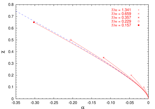
Figure 2: Finite temperature PW flows away from the UV stable fixed point $(\alpha,\chi)=(0,0)$. The endpoints of the flows correspond to the fixed values of the scalars at the horizon. The dashed line gives the supersymmetric zero-temperature flow.

We recall that at zero temperature the PW flow involves the scalars $\rho$ and $\chi$ running away from the UV fixed point as one flows to the IR. At a regular horizon, the scalars attain fixed values $\rho_{0}$ and $\chi_{0}$. Hence we now seek a solution to (3.17) satisfying the conditions

$$(\rho,\chi)\to(1,0)\quad\hbox{as}\quad y\to 1_{-}\,,\qquad(\rho,\chi)\to(\rho_{0},\chi_{0})\quad\hbox{as}\quad y\to 0\,.$$ (5.4)

Several flows satisfying these boundary conditions are displayed in Fig. 2. It is clear from the figure that the flows proceed further into the IR as the temperature is lowered. While we have been unable to find an exact analytical solution, it is nevertheless possible to develop a consistent (uniformly convergent) perturbative approximation in the high temperature phase. On the gauge theory side, this corresponds to a power series expansion in $\alpha_{1}\propto(m_{b})^{2}\ll 1$ and $\alpha_{2}\propto m_{f}\ll 1$, where $m_{b}$ and $m_{f}$ are masses of the bosonic and fermionic components of the ${\cal N}=2$ hypermultiplet measured with respect to the string scale. In what follows, we solve for the leading order deformation in $\alpha_{1}$ and $\alpha_{2}$. Specifically, we seek a solution of (3.17) in the form

$$\begin{split}A(y)&=\hat{\alpha}-\frac{1}{4}\ln(1-y^{2})+\alpha_{1}^{2}A_{1}(y)+\alpha_{2}^{2}A_{2}(y)\,,\\ \rho(y)&=1+\alpha_{1}\rho_{1}(y)\,,\\ \chi(y)&=\alpha_{2}\chi_{2}(y)\,.\end{split}$$ (5.5)

Substituting this ansatz into (3.17), and working to first non-trivial order in $\alpha_{i}$, we find the linearized scalar equations

$$\begin{split}0&=(1-y^{2})^{2}\,\left(y\,\rho_{1}^{\prime}\right)^{\prime}+y\,\rho_{1}\,,\\ 0&=(1-y^{2})^{2}\,\left(y\,\chi_{2}^{\prime}\right)^{\prime}+\frac{3}{4}\,y\,\chi_{2}\,,\\ \end{split}$$ (5.6)

as well as the equations governing the back-reaction on the metric

$$\begin{split}0&=y(1-y^{2})\,A_{1}^{\prime\prime}-(1+3y^{2})\,A_{1}^{\prime}+4y(1-y^{2})\,\left(\rho_{1}^{\prime}\right)^{2}\,,\\ 0&=y(1-y^{2})\,A_{2}^{\prime\prime}-(1+3y^{2})\,A_{2}^{\prime}+\frac{4}{3}y(1-y^{2})\,\left(\chi_{2}^{\prime}\right)^{2}\,.\end{split}$$ (5.7)

The scalar equations, (5.6), may equally well be obtained from the linearization of (3.15). Note that for an arbitrary scalar $\Phi(y)$ of mass $m$, its equation of motion, $\mathop{\mathchoice{{\vbox{\vbox{\hrule height=0.32pt\hbox{\vrule width=0.32pt,height=8.0pt\kern 8.0pt\vrule width=0.32pt}\hrule height=0.32pt}}}}{{\vbox{\vbox{\hrule height=0.32pt\hbox{\vrule width=0.32pt,height=8.0pt\kern 8.0pt\vrule width=0.32pt}\hrule height=0.32pt}}}}{{\vbox{\vbox{\hrule height=0.9pt\hbox{\vrule width=0.9pt,height=6.3pt\kern 6.3pt\vrule width=0.9pt}\hrule height=0.9pt}}}}{{\vbox{\vbox{\hrule height=0.9pt\hbox{\vrule width=0.9pt,height=4.5pt\kern 4.5pt\vrule width=0.9pt}\hrule height=0.9pt}}}}}\Phi=m^{2}\Phi$, in the background (5.2) has the form

$$\Phi^{\prime\prime}+{\frac{1}{y}}\Phi^{\prime}={\frac{(mL)^{2}}{4(1-y^{2})^{2}}}\Phi\,.$$ (5.8)

This may be readily solved in terms of hypergeometric functions. Although there are generally two linearly independent solutions, only one combination is regular at the horizon, $y\to 0$. Defining $E_{0}=2\pm\sqrt{4+(mL)^{2}}$, the regular solution has the form

$$\Phi=(1-y^{2})^{E_{0}/4}{}_{2}F_{1}({\textstyle{\frac{1}{4}}}E_{0},{\textstyle{\frac{1}{4}}}E_{0},1;y^{2})\,.$$ (5.9)

As a result, for the $\rho$ and $\chi$ scalars, we obtain

$$\begin{split}\rho_{1}&=(1-y^{2})^{1/2}\ _{2}F_{1}({\textstyle{\frac{1}{2}}},{\textstyle{\frac{1}{2}}},1;y^{2})\,,\\ \chi_{2}&=(1-y^{2})^{3/4}\ _{2}F_{1}({\textstyle{\frac{3}{4}}},{\textstyle{\frac{3}{4}}},1;y^{2})\,,\end{split}$$ (5.10)

where, without loss of generality, we assumed the horizon boundary conditions

$$\rho_{1}\bigg{|}_{y=0}=1\,,\qquad\chi_{2}\bigg{|}_{y=0}=1\,.$$ (5.11)

Note that as $y\to 1_{-}$, the perturbations $\rho_{1},\ \chi_{2}$ vanish. This is readily seen by rewriting the solution, (5.9), as

$$\begin{split}\Phi=&{\frac{\Gamma(1-{\frac{1}{2}}E_{0})}{\Gamma(1-{\frac{1}{4}}E_{0})}}(1-y^{2})^{E_{0}/4}{}_{2}F_{1}({\textstyle{\frac{1}{4}}}E_{0},{\textstyle{\frac{1}{4}}}E_{0},{\textstyle{\frac{1}{2}}}E_{0};1-y^{2})\\ &+{\frac{\Gamma({\frac{1}{2}}E_{0}-1)}{\Gamma({\frac{1}{4}}E_{0})}}(1-y^{2})^{(4-E_{0})/4}{}_{2}F_{1}(1-{\textstyle{\frac{1}{4}}}E_{0},1-{\textstyle{\frac{1}{4}}}E_{0},2-{\textstyle{\frac{1}{2}}}E_{0};1-y^{2})\,,\end{split}$$ (5.12)

which is valid provided $E_{0}\neq 2$. Expanding for $y\to 1_{-}$ yields the expected boundary behavior, $\Phi\sim(1-y)^{\Delta_{+}/4}$ and $(1-y)^{\Delta_{-}/4}$, where the conformal dimensions $\Delta_{\pm}$ correspond to $E_{0}$ and $4-E_{0}$. In this case, however, instead of being independent, the $\Delta_{+}$ and $\Delta_{-}$ modes are related by the condition of horizon regularity.

Turning to the leading order gravitational back-reaction, we see that (5.7) can be solved by quadratures

$$\begin{split}A_{1}&=\xi_{1}-4\int_{0}^{y}\,\frac{z\,dz}{(1-z^{2})^{2}}\ \biggl{(}\gamma_{1}+\int_{0}^{z}dx\,\left(\frac{\partial\rho_{1}}{\partial x}\right)^{2}\,\frac{(1-x^{2})^{2}}{x}\biggr{)}\,,\\[4.0pt] A_{2}&=\xi_{2}-\frac{4}{3}\int_{0}^{y}\,\frac{z\,dz}{(1-z^{2})^{2}}\ \biggl{(}\gamma_{2}+\int_{0}^{z}dx\,\left(\frac{\partial\chi_{2}}{\partial x}\right)^{2}\,\frac{(1-x^{2})^{2}}{x}\biggr{)}\,,\\ \end{split}$$ (5.13)

where $\gamma_{i},\ \xi_{i}$ are four integration constants. For a generic choice of $\gamma_{i}$, we find $A_{i}|_{y\to 1_{-}}\propto(1-y)^{-1}$; thus to recover the proper asymptotics in the UV $AdS_{5}\times S^{5}$ geometry, these constants must be fine tuned:

$$\gamma_{1}=\frac{8-\pi^{2}}{2\pi^{2}}\,,\qquad\gamma_{2}=\frac{8-3\pi}{8\pi}\,.$$ (5.14)

The other two integration constants, $\xi_{i}$, can be absorbed in a redefinition of $\hat{\alpha}$. In fact, we show below that the physical quantities are $\xi_{i}$ independent. Note that at the horizon we have the behavior

$$\left(\frac{\partial y}{\partial r}\right)^{2}\bigg{|}_{y\to 0_{+}}\!\!=\delta^{2}\ \sim\ 1+4\alpha_{1}^{2}\left(1+2\gamma_{1}\right)+\alpha_{2}^{2}\left(1+\frac{8}{3}\gamma_{2}\right)\,.$$ (5.15)

This allows us to compute the BH temperature

$$T=\frac{1}{2\pi}e^{A}\left(\frac{\partial y}{\partial r}\right)\bigg{|}_{y\to 0_{+}}\!\!=\frac{1}{2\pi}e^{\alpha}\,\delta\sim\frac{1}{2\pi}e^{\hat{\alpha}}\,\biggl{(}1+\alpha_{1}^{2}\left(2+\xi_{1}+4\gamma_{1}\right)+\frac{1}{6}\alpha_{2}^{2}\left(3+6\xi_{2}+8\gamma_{2}\right)\biggr{)}.$$ (5.16)

While the first relation is valid for arbitrary temperature and masses, in the second one we have kept only the leading terms in $\alpha_{i}$.

Using the explicit lifting of the metric, (4.12), we may compute the area of the BH horizon

$$\begin{split}{\cal A}_{horizon}=V_{3}\ e^{3A}\bigg{|}_{y\to 0_{+}}\!\!&=V_{3}\ e^{3\alpha}\\ &\sim V_{3}\ e^{3\hat{\alpha}}\ 2^{5}{\rm vol}_{S^{5}}\,\left(1+3\xi_{1}\alpha_{1}^{2}+3\xi_{2}\alpha_{2}^{2}\right)\,,\end{split}$$ (5.17)

where $V_{3}$ is the 3-dimensional volume and ${\rm vol}_{S^{5}}$ is the volume of the unit $S^{5}$. Again, the first relation in (5.17) is exact for all temperatures/masses. The Bekenstein-Hawking entropy density is

$$S_{BH}=\frac{{\cal A}_{horizon}}{4G_{N}}=\frac{1}{2}\,\pi^{2}N^{2}\,\left(\frac{1}{2\pi}\ e^{\alpha}\right)^{3}\sim\frac{1}{2}\,\pi^{2}N^{2}\,\left(\frac{1}{2\pi}\ e^{\hat{\alpha}}\right)^{3}\left(1+3\xi_{1}\alpha_{1}^{2}+3\xi_{2}\alpha_{2}^{2}\right)\,.$$ (5.18)

6 Thermodynamics and the signature of the phase transition

In this section we discuss the thermodynamic properties of the $N=2^{*}$ theory. As we have explained above, physically we expect a phase transition between the deconfining phase (at high temperature) and the finite temperature Coulomb phase (at low temperature). The high temperature phase is realized by the BH geometry, represented by the solution to (3.17) with boundary conditions (3.20). The low temperature phase is the $\gamma=0$ (Euclidean) PW geometry [13] with periodically identified (Euclidean) time direction $t_{E}\sim t_{E}+1/T$.

We begin by considering the standard definition (and regularization) of the free energy and the energy of the finite temperature deformed PW background. Specifically, we identify the Helmholtz free energy $F$ with the combination $T\,I^{renom}_{E}$, where $I^{renom}_{E}$ is the renormalized Euclidean gravitational action, and the dual gauge theory energy $E$ with the ADM mass of the finite temperature deformed PW geometry. Also, we identify the gauge theory entropy with the Bekenstein-Hawking entropy of the deformed PW background. We show that, with such identifications, we identically satisfy the thermodynamic relation $F=E-TS$. This extraction of the thermodynamic quantities are valid for arbitrary values of mass and temperature.

To proceed, we note that supersymmetry of the PW background relates the $\alpha_{1}$ and $\alpha_{2}$ coefficients of the leading nontrivial asymptotic behavior of the five-dimensional scalars $\rho$ and $\chi$. This allows us to parametrize the thermal phase of PW by the single quantity $m/T$. In the high temperature phase, we analytically compute the leading correction to the near extremal D3 brane thermodynamics due to the PW mass deformation. The sign of this correction to the black D3 branes is consistent with our claim for a phase transition.

We find that, in the high temperature phase, our extracted free energy no longer satisfies $dF=-SdT$, thus apparently violating the first law of thermodynamics. We provide a possible resolution to this puzzle in terms of a generalized chemical potential induced by the PW mass deformation. However a full understanding of the thermodynamics requires additional investigation.

6.1 The regularized free energy and the energy

We recall that the free energy $F$, the energy $E$, and the entropy $S$ of the a system is related by the well known expression

$$F=E-TS\,.$$ (6.1)

Here, $F$, $E$ and $S$ are well defined quantities in a weakly coupled gauge theory, and physically should remain well defined (finite) at large ’t Hooft coupling. It is known, however, that in the dual supergravity both the free energy and energy densities are divergent, and thus need to be properly renormalized before they can yield a finite answer. A standard regulating procedure is to compute such quantities by comparison with a ’reference’ supergravity background having the same asymptotics. This comparison is often ad hoc; in particular, the matching of the two geometries at hand at the regularization boundary remains slightly ambiguous. In our case, however, we have a physically well motivated reference geometry, namely the PW background with periodic Euclidean time direction of appropriate size.

Using the PW background as reference, strictly speaking we will not be computing $F_{BH}$, $E_{BH}$ and $S_{BH}$ directly [where the subscript _BH relates to the non extremal deformation (3.16)–(3.20)], but rather the differences

$$\Delta F\equiv\,F_{BH}-F_{PW}\,,\qquad\Delta E\equiv\,E_{BH}-E_{PW}\,,\qquad\Delta S\equiv\,S_{BH}-S_{PW}\,.$$ (6.2)

In practice, we expect these quantities to be dominated by their _BH values, $\Delta F=F_{BH}$, $\Delta E=E_{BH}$, $\Delta S=S_{BH}$. This is clearly the case at weak ’t Hooft coupling since the thermodynamic quantities in the finite temperature Coulomb phase are $1/N$ down compared to the corresponding quantities in the deconfined phase, and thus the former are essentially zero in the large $N$ limit. Experience with other examples of the gauge/gravity correspondence suggests that going to strong ’t Hooft coupling would typically modify the prefactor, but not the large $N$ scaling of the free energy, the energy and the entropy. Note that the choice of PW background as a reference one is particularly convenient when exploring the phase transition, as a phase transition implies going through a zero in $\Delta F$ in (6.2) as one changes the temperature.

Before proceeding to the BH solution, we recall the asymptotics of the reference PW geometry. In [13] the solution of the supersymmetric $\gamma=0$ flow equations is given in terms of $\chi$ as the flow coordinate:

$$\begin{split}e^{A}&=\frac{k\rho^{2}}{\sinh(2\chi)}\,,\\ \rho^{6}&=\cosh(2\chi)+\sinh^{2}(2\chi)\,\ln\frac{\sinh(\chi)}{\cosh(\chi)}\,.\end{split}$$ (6.3)

The single integration constant $k$ in (6.3) is related to the hypermultiplet mass $m$ in (3.1) by [14]

$$k=mL=2m\,.$$ (6.4)

As indicated in (3.12) and (3.13), the scalars $(\rho,\chi)$ start at their UV fixed point $(1_{-},0_{+})$, and flow toward $(0_{+},+\infty)$ in the IR. Using the the flow equations, (3.11), we find the IR asymptotics

$$\begin{split}\ln\rho&\sim-{\frac{1}{3}}\chi+{\frac{1}{6}}\ln{\frac{4}{3}}\,,\\ e^{A}&\sim 2k\,(4/3)^{1/3}\,e^{-8\chi/3}\,,\\ \frac{dA}{dr}&\sim(4/3)^{2/3}\,e^{2\chi/3}\,.\end{split}$$ (6.5)

For matching, we are more interested in the UV behavior. To develop the asymptotics at the boundary, we introduce

$$\hat{x}\equiv e^{-r/2}\,.$$ (6.6)

We find in the UV

$$\begin{split}\chi&\sim k\hat{x}\left[1+k^{2}\hat{x}^{2}\left({\textstyle{\frac{1}{3}}}+{\textstyle{\frac{4}{3}}}\ln(k\hat{x})\right)+k^{4}\hat{x}^{4}\left(-{\textstyle{\frac{7}{90}}}+{\textstyle{\frac{10}{3}}}\ln(k\hat{x})+{\textstyle{\frac{20}{9}}}\ln^{2}(k\hat{x})\right)\right]\,,\\[8.0pt] \rho&\sim 1+k^{2}\hat{x}^{2}\left({\textstyle{\frac{1}{3}}}+{\textstyle{\frac{2}{3}}}\ln(k\hat{x})\right)+k^{4}\hat{x}^{4}\left({\textstyle{\frac{1}{18}}}+2\ln(k\hat{x})+{\textstyle{\frac{2}{3}}}\ln^{2}(k\hat{x})\right)\,,\\[8.0pt] A&\sim-\ln(2\hat{x})-{\textstyle{\frac{1}{3}}}k^{2}\hat{x}^{2}-k^{4}\hat{x}^{4}\left({\textstyle{\frac{2}{9}}}+{\textstyle{\frac{10}{9}}}\ln(k\hat{x})+{\textstyle{\frac{4}{9}}}\ln^{2}(k\hat{x})\right)\,,\\[8.0pt] \frac{dA}{dr}&\sim{\textstyle{\frac{1}{2}}}+{\textstyle{\frac{1}{3}}}k^{2}\hat{x}^{2}+k^{4}\hat{x}^{4}\left(1+{\textstyle{\frac{8}{3}}}\ln(k\hat{x})+{\textstyle{\frac{8}{9}}}\ln^{2}(k\hat{x})\right)\,.\end{split}$$ (6.7)

Note that, as will be evident later, we need to keep terms up to ${\cal O}(\hat{x}^{4})$ in the expansion.

Turning now to the BW geometry, the general solution of (3.17) which is smooth in the IR ($e^{B}\to 0$) has three integration constants, $\{\alpha,\chi_{0},\rho_{0}\}$, which are related to temperature and masses of the ${\cal N}=2$ hypermultiplet components, (3.20), (3.21). The most general solution of (3.17) in the UV ($\chi\to 0_{+}$) has altogether five parameters, $\{\xi,\hat{\rho}_{10},\hat{\rho}_{11},\hat{\chi}_{0},\hat{\chi}_{10}\}$. Three of them are related to the temperature and the masses, while the other two are uniquely determined from the requirement of having a regular horizon, (3.21). In any case, we have a three parameter BH solution

$$\begin{split}B\sim\,&-\beta\,x^{4}\bigl{[}1+{\textstyle{\frac{8}{9}}}x^{2}\hat{\chi}_{0}^{2}+x^{4}\bigl{(}{\textstyle{\frac{5}{16}}}\hat{\rho}_{11}^{2}-{\textstyle{\frac{1}{2}}}\hat{\rho}_{11}\hat{\rho}_{10}+{\textstyle{\frac{1}{18}}}\hat{\chi}_{0}^{4}+2\hat{\rho}_{10}^{2}+\hat{\chi}_{0}^{2}\hat{\chi}_{10}\\ &\qquad+\ln x\left(-{\textstyle{\frac{1}{2}}}\hat{\rho}_{11}^{2}+{\textstyle{\frac{4}{3}}}\hat{\chi}_{0}^{4}+4\hat{\rho}_{11}\hat{\rho}_{10}\right)+2\hat{\rho}_{11}^{2}\ln^{2}x\bigr{)}\bigr{]}\,,\\[8.0pt] \chi\sim\,&\hat{\chi}_{0}\,x\,\bigl{[}1+x^{2}\left(\hat{\chi}_{10}+{\textstyle{\frac{4}{3}}}\hat{\chi}_{0}^{2}\ \ln x\right)+x^{4}\bigl{(}{\textstyle{\frac{31}{8}}}\hat{\rho}_{11}^{2}-{\textstyle{\frac{13}{2}}}\hat{\rho}_{11}\hat{\rho}_{10}-{\textstyle{\frac{56}{45}}}\hat{\chi}_{0}^{4}-{\textstyle{\frac{3}{2}}}\hat{\chi}_{0}^{2}\hat{\rho}_{11}+2\hat{\chi}_{0}^{2}\hat{\rho}_{10}\\ &\qquad+5\hat{\rho}_{10}^{2}+2\hat{\chi}_{0}^{2}\hat{\chi}_{10}+\ln x\left(-{\textstyle{\frac{13}{2}}}\hat{\rho}_{11}^{2}+10\hat{\rho}_{11}\hat{\rho}_{10}+{\textstyle{\frac{8}{3}}}\hat{\chi}_{0}^{4}+2\hat{\chi}_{0}^{2}\hat{\rho}_{11}\right)+5\hat{\rho}_{11}^{2}\ln^{2}x\bigr{)}\bigr{]}\,,\\[8.0pt] \rho\sim\,&1+x^{2}\left(\hat{\rho}_{10}+\hat{\rho}_{11}\ln x\right)+x^{4}\bigl{(}-2\hat{\rho}_{11}\hat{\rho}_{10}+{\textstyle{\frac{3}{2}}}\hat{\rho}_{11}^{2}+{\textstyle{\frac{3}{2}}}\hat{\rho}_{10}^{2}+{\textstyle{\frac{10}{3}}}\hat{\chi}_{0}^{2}\hat{\rho}_{10}-{\textstyle{\frac{8}{3}}}\hat{\chi}_{0}^{2}\hat{\rho}_{11}+{\textstyle{\frac{1}{3}}}\hat{\chi}_{0}^{4}\\ &\qquad+\ln x\left(3\hat{\rho}_{11}\hat{\rho}_{10}+{\textstyle{\frac{10}{3}}}\hat{\chi}_{0}^{2}\hat{\rho}_{11}-2\hat{\rho}_{11}^{2}\right)+{\textstyle{\frac{3}{2}}}\hat{\rho}_{11}^{2}\ln^{2}x\bigr{)}\,,\\[8.0pt] A\sim\,&\xi-\ln x-{\textstyle{\frac{1}{3}}}\hat{\chi}_{0}^{2}x^{2}+x^{4}\bigl{(}{\textstyle{\frac{1}{4}}}\beta+{\textstyle{\frac{1}{9}}}\hat{\chi}_{0}^{4}-{\textstyle{\frac{1}{2}}}\hat{\chi}_{0}^{2}\hat{\chi}_{10}-{\textstyle{\frac{1}{8}}}\hat{\rho}_{11}^{2}-\hat{\rho}_{10}^{2}\\ &\qquad-\ln x\left({\textstyle{\frac{2}{3}}}\hat{\chi}_{0}^{4}+2\hat{\rho}_{11}\hat{\rho}_{10}\right)-\hat{\rho}_{11}^{2}\ln^{2}x\bigr{)}\,,\end{split}$$ (6.8)

Here we have introduced an additional integration constant $\beta$ which, however, can be absorbed at the expense of shifting the position of the horizon in the radial coordinate $r$ (or alternatively by rescaling $x$). For this reason, $\beta$ should not be considered an independent parameter of the solution. Also, we find

$$\begin{split}\frac{dA}{dr}\sim\ &{\textstyle{\frac{1}{2}}}+{\textstyle{\frac{1}{3}}}\hat{\chi}_{0}^{2}x^{2}+x^{4}\bigl{(}-{\textstyle{\frac{1}{2}}}\beta+2\hat{\rho}_{10}^{2}+\hat{\rho}_{11}\hat{\rho}_{10}+{\textstyle{\frac{1}{4}}}\hat{\rho}_{11}^{2}+\hat{\chi}_{0}^{2}\hat{\chi}_{10}+{\textstyle{\frac{1}{9}}}\hat{\chi}_{0}^{4}\\ &+\ln x\left(\hat{\rho}_{11}^{2}+{\textstyle{\frac{4}{3}}}\hat{\chi}_{0}^{4}+4\hat{\rho}_{11}\hat{\rho}_{10}\right)+2\hat{\rho}_{11}^{2}\ln^{2}x\bigr{)}\,.\end{split}$$ (6.9)

In (6.8) and (6.9), $x=x_{0}e^{-r/2}$ with $x_{0}$ an arbitrary constant.

The free energy, $F$, of the gravitational action can be obtained from the (Euclidean) action $I_{E}$ according to

$$F=T\,I_{E}=\frac{1}{2\pi}\,e^{\alpha}\,\delta\,I_{E}[\alpha,\chi_{0},\rho_{0}]\,,$$ (6.10)

where $T$ is the temperature. As usual, $I_{E}$ is divergent and should be properly regularized. As explained above, our approach is to regulate the free energy by subtraction, $\Delta F=T\Delta I_{E}$, where

$$\Delta I_{E}[\alpha,\chi_{0},\rho_{0}]=\lim_{r\to\infty}\ \biggl{\{}I_{BH}^{r}[\alpha,\chi_{0},\rho_{0}]-I_{PW}^{r}[T,k]\biggr{\}}\,.$$ (6.11)

The regularized action $I_{E}^{r}$ consists of both volume and surface terms

$$\begin{split}I_{E}^{r}=&I^{r}_{\rm bulk}+I^{r}_{\rm surf}\\ =&\frac{1}{4\pi G_{5}}\int^{r}\!dr\int_{\partial{\cal M}_{5}}\!d^{4}\xi\,\sqrt{g^{E}}\left(-{\textstyle{\frac{1}{4}}}R^{E}+(\partial\alpha)^{2}+(\partial\chi)^{2}+{\cal P}\right)\\ &-\frac{1}{8\pi G_{5}}\int_{\partial{\cal M}_{5}}\!d^{4}\xi\,\sqrt{h^{E}}\ \nabla_{\mu}n^{\mu}\,,\end{split}$$ (6.12)

where $G_{5}$ is the five dimensional Newton’s constant

$$G_{5}\equiv\frac{G_{N}}{2^{5}\ {\rm vol}_{S^{5}}}=\frac{4\pi}{N^{2}}\,,$$ (6.13)

$g^{E}$ is the Euclidean version of the metric (3.16), $n^{\mu}$ is a unit vector orthogonal to the four-dimensional boundary $\partial{\cal M}_{5}$, and $h^{E}_{\mu\nu}$ is the induced metric on $\partial{\cal M}_{5}$

$$h^{E}_{\mu\nu}=g^{E}_{\mu\nu}+n_{\mu}n_{\nu}\,.$$ (6.14)

In (6.11) we have assumed that the boundary $\partial{\cal M}_{5}$ is defined at fixed $r$ [in the coordinates (3.16)], which we will take to infinity at the end of the calculations. In this case, the unit normal vector is $n^{\mu}=\delta^{\mu}_{r}$.

Consider first the bulk contribution in (6.12). Because of local diffeomorphism invariance, the on-shell value of the action must reduce to a surface integral. This is indeed what we find:

$$\begin{split}I^{r}_{\rm bulk}=&\frac{1}{4\pi G_{5}}\int^{r}dr\,\sqrt{g^{E}}\,\left(-{\textstyle{\frac{2}{3}}}{\cal P}\right)\\ =&\frac{1}{4\pi G_{5}}\int^{r}dr\ \left({\textstyle{\frac{1}{2}}}\,e^{3A}\,\left(e^{A+B}\right)^{\prime}+\upsilon\,e^{4A}\left(e^{B}\right)^{\prime}\right)^{\prime}\,,\end{split}$$ (6.15)

where $\upsilon$ is an arbitrary constant parameterizing the constraint (3.19). In what follows, we find it convenient to set

$$\upsilon=0\,.$$ (6.16)

In this case

$$I^{r}_{bulk}=\frac{1}{8\pi G_{5}}\,e^{3A}\left(e^{A+B}\right)^{\prime}\bigg{|}_{horizon}^{r}\,,$$ (6.17)

where ${horizon}$ refers to either the standard black hole horizon location for the “deconfining phase” (BH) analytically continued to Euclidean signature or the IR ($\chi\to+\infty$) of the Euclidean PW solution with periodically identified time direction (PW). Notice that at the black hole horizon

$$\frac{1}{8\pi G_{5}}\,e^{3A}\left(e^{A+B}\right)^{\prime}\bigg{|}_{horizon,\ BH}=\frac{1}{8\pi G_{5}}\,e^{4A}\ \frac{\partial y}{\partial r}\bigg{|}_{horizon,\ BH}=S_{BH}T\,,$$ (6.18)

where $S_{BH}$ is exactly the black hole entropy (5.18), and $T$ is the corresponding black hole temperature (5.16). On the other hand, using the IR asymptotics of the PW solution, (6.5), we find instead

$$\frac{1}{8\pi G_{5}}\,e^{3A}\left(e^{A}\right)^{\prime}\bigg{|}_{horizon,\ PW}=0=S_{PW}T\,,$$ (6.19)

which is simply interpreted in terms of the vanishing entropy of the PW phase.

It should be noted that the black hole horizon is a regular point of the Euclidean geometry. Thus it is unusual to find a horizon surface term contribution to the Euclidean bulk action (6.15). In fact, this contribution is somewhat artificial, and arises because of our particular choice of $\upsilon$, (6.16). Indeed, for generic $\upsilon$, we find

$$\left[\frac{1}{8\pi G_{5}}\,e^{3A}\left(e^{A+B}\right)^{\prime}+\frac{\upsilon}{4\pi G_{5}}\,e^{4A+B}B^{\prime}\right]\bigg{|}_{horizon}=\frac{1+2\upsilon}{8\pi G_{5}}\ e^{4A+B}B^{\prime}\bigg{|}_{horizon}\,,$$ (6.20)

where we have used the fact that $e^{3A+B}(e^{A})^{\prime}|_{horizon}=0$ for both the $BH$ and the $PW$ phases. From (6.20) we see that for $\upsilon=-1/2$, the full contribution to $I^{r}_{bulk}$, (6.15), would come from the asymptotic region. Although, strictly speaking, this is the only proper value for $\upsilon$, since the full value of the Euclidean action (6.15) is independent of $\upsilon$, we nevertheless find it convenient to retain $\upsilon=0$, as indicated in (6.16).

For the surface term in (6.12), we find

$$I^{r}_{surf}=-\frac{1}{8\pi G_{5}}\ \left(e^{4A+B}\right)^{\prime}\bigg{|}^{r}\,.$$ (6.21)

Adding the bulk (6.17) and the surface (6.21) terms together, we find

$$I_{E}^{r}=-\frac{1}{8\pi G_{5}}e^{3A}\left(e^{A+B}\right)^{\prime}\bigg{|}_{horizon}-\frac{3}{8\pi G_{5}}e^{4A+B}\ A^{\prime}\bigg{|}^{r}\,.$$ (6.22)

We have shown above that the first term in (6.22) is simply the combination $-ST$ where $S$ is the entropy density. If the standard relation (6.1) is realized in the supergravity (and it must be so), then the other term in (6.22) must be the regularized energy density. Indeed this is so, provided we define the (regularized) ADM energy density of the background as

$$E\,V_{3}=\lim_{r\to\infty}\left\{E^{r}\,V_{3}\right\}=\lim_{r\to\infty}\left\{-\frac{1}{8\pi G_{5}}\int_{v_{3}(r)}\sqrt{-g_{tt}}\ {}^{2}K_{v_{3}}\,dv_{3}(r)\right\}\,,$$ (6.23)

where the 3-boundary $v_{3}(r)$ is the spacelike foliation of $\partial{\cal M}_{5}$ and ${}^{2}K_{v_{3}}$ is its extrinsic curvature. Explicit evaluation of (6.23) yields

$$E^{r}=-\frac{3}{8\pi G_{5}}\,e^{4A+B}\ A^{\prime}\bigg{|}^{r}\,,$$ (6.24)

which is indeed the second term of (6.22).

Having derived the general asymptotic expansions for the black hole and the PW geometry in (6.7) and (6.8), we are now ready to evaluate $\Delta F$:

$$\begin{split}F_{BH}-F_{PW}=&-\left(S_{BH}-S_{PW}\right)T+\left(E_{BH}-E_{PW}\right)\\ =&\frac{1}{8\pi G_{5}}\biggl{\{}-e^{4A}\frac{\partial y}{\partial r}\bigg{|}_{horizon,\ BH}-3\ \lim_{r\to\infty}\left[e^{4A+B}A^{\prime}\bigg{|}_{BH}-e^{4A+B}A^{\prime}\bigg{|}_{PW}\right]\biggr{\}}\\ =&\frac{1}{8\pi G_{5}}\biggl{\{}-e^{4\alpha}\ \delta-3\ \Delta_{PW}^{BH}\biggr{\}}\,,\end{split}$$ (6.25)

where in the last line we have used (3.20). The evaluation of the limit in (6.25) is rather simple. We choose a direct matching condition of the $BH$ and $PW$ boundaries, parameterized by $x$ [see (6.8) and (6.9)] and $\hat{x}$ [see (6.7)] respectively:

$$\hat{x}=\delta_{0}\ x\,.$$ (6.26)

Additionally we have to set

$$B\bigg{|}_{PW}=0\,.$$ (6.27)

Matching the boundary values of the scalars $\rho$ and $\chi$ for the black hole and reference geometries yields

$$\hat{\rho}_{11}=\frac{2}{3}\ k^{2}\ \delta_{0}^{2},\qquad\hat{\chi}_{0}=k\ \delta_{0}\,.$$ (6.28)

Furthermore, matching the asymptotic volumes of the $BH$ and $PW$ phases determines

$$\delta_{0}=\frac{1}{2}e^{-\xi}\,.$$ (6.29)

The final result is

$$\begin{split}\Delta^{BH}_{PW}&=e^{4\xi}\biggl{(}-\frac{\beta}{2}+\frac{1}{6}\ \eta^{2}\hat{\rho}_{10}-\frac{1}{72}\ \eta^{4}\ln\left(\frac{1}{4}\ e\ \eta^{2}\right)\biggr{)}\,,\end{split}$$ (6.30)

where we have introduced

$$\eta\equiv ke^{-\xi}\,.$$ (6.31)

The difference of free energies thus has the form

$$\begin{split}F_{BH}-F_{PW}&=-\frac{e^{4\alpha}}{8\pi G_{5}}\ \biggl{(}\delta+3\,e^{-4\alpha}\Delta^{BH}_{PW}\biggr{)}\\ &=-\frac{\pi^{2}N^{2}}{2}\ \left(\frac{1}{2\pi}\ e^{\alpha}\right)^{4}\biggl{(}\delta+3\ e^{-4\alpha}\Delta^{BH}_{PW}\biggr{)}\,.\end{split}$$ (6.32)

This can be further simplified by using the integral of motion, (3.19). Indeed, evaluating the constant in (3.19) in the IR and the UV, and equating them, we find

$$\ln\beta+\ln 2+4\xi=4\alpha+\ln\delta\,.$$ (6.33)

Thus we can rewrite (6.32) as

$$\begin{split}F_{BH}-F_{PW}=-\frac{\pi^{2}N^{2}}{4(2\pi)^{4}}\,e^{4\xi}\,\biggl{(}\beta+\eta^{2}\hat{\rho}_{10}-\frac{1}{12}\,\eta^{4}\,\ln\left(\frac{1}{4}\,e\,\eta^{2}\right)\biggr{)}\,.\end{split}$$ (6.34)

Notice that from (6.8) the residual reparametrization invariance $x\to\lambda x$ can be absorbed by the following transformation on the quantities $\{\xi,\hat{\rho}_{10},\hat{\rho}_{11},\hat{\chi}_{0},\hat{\chi}_{10},\beta\}$:

$$\begin{split}\xi&\to\xi-\ln\lambda\,,\\ \hat{\rho}_{10}&\to\lambda^{2}\hat{\rho}_{10}+\lambda^{2}\hat{\rho}_{11}\ln\lambda\,,\qquad\hat{\rho}_{11}\to\lambda^{2}\hat{\rho}_{11}\,,\\ \hat{\chi}_{0}&\to\lambda\hat{\chi}_{0}\,,\kern 78.00014pt\hat{\chi}_{10}\to\lambda^{2}\hat{\chi}_{10}+\frac{4}{3}\lambda^{2}\hat{\chi}_{0}^{2}\ln\lambda\,,\\ \beta&\to\lambda^{4}\beta\,.\end{split}$$ (6.35)

This leaves (6.34) invariant.

From the gauge theory arguments, we expect that the free energy of the $PW$ phase scales as $N^{1}$. On the other hand, the $N$-scaling in (6.34) suggests that in the large $N$-limit, $F_{PW}$ is essentially zero compared to $F_{BH}$. Thus, in the high temperature phase, we identify the ${\cal N}=2^{*}$ gauge theory Helmholtz free energy density $F$ at large ’t Hooft coupling with (6.34)

$$\begin{split}F\equiv F_{BH}-F_{PW}&\equiv T\,I_{E}^{renom}\\ &=-\frac{\pi^{2}N^{2}}{4(2\pi)^{4}}\,e^{4\xi}\,\biggl{(}\beta+\eta^{2}\hat{\rho}_{10}-\frac{1}{12}\,\eta^{4}\,\ln\left(\frac{1}{4}\,e\,\eta^{2}\right)\biggr{)}\,.\end{split}$$ (6.36)

Also, from (5.18) and (6.33), the ${\cal N}=2^{*}$ gauge theory entropy density $S$ is

$$S\equiv S_{BH}=\frac{N^{2}}{8(2\pi)}\,e^{3\alpha}=\frac{N^{2}}{8(2\pi)}\,\left(\frac{2\beta}{\delta}\right)^{3/4}\,e^{3\xi}\,.$$ (6.37)

Finally, the gauge theory energy density $E$ is that of the (renormalized) ADM energy density [from (6.25)]

$$E\equiv E_{BH}-E_{PW}=T\,I_{E}^{renom}+T\,S_{BH}\,.$$ (6.38)

The gauge theory temperature $T$ is identified with that of the horizon in the $BH$ phase, (5.16).

6.2 The high temperature thermodynamics of the ${\cal N}=2^{*}$

Given the analytical expression for the high temperature expansion, (5.5)–(5.14), it is straightforward to determine the leading correction to the non-extremal D3 brane thermodynamics due to the PW mass flow. As we will note, the sign of this correction suggests the possibility of the “deconfinement $\rightarrow$ finite temperature Coulomb phase” phase transition.

We begin by matching the $\{\hat{\alpha},\alpha_{1},\alpha_{2}\}$ parameters in (5.5) with $\{\xi,\hat{\chi},\hat{\rho}\}$ of the asymptotic expansion, (6.8). Recall that the $y$ coordinate in (5.10) is just $e^{B}$. Thus the $x$ coordinate of (6.8) and $y$ are related according to

$$y\sim\ 1-2x^{4}\,.$$ (6.39)

This corresponds to setting $\beta=2$ in (6.8). Now, to linear order in $\alpha_{i}$, by matching the scalars $\rho$, $\chi$ in (5.10) and (6.8), we find

$$\begin{split}\hat{\rho}_{10}&=\frac{4\ln 2}{\pi}\,\alpha_{1}\,,\qquad\qquad\quad\,\hat{\rho}_{11}=-\frac{8}{\pi}\,\alpha_{1}\,,\\ \hat{\chi}_{0}&=\frac{\sqrt{2\pi}}{[\Gamma\left(\frac{3}{4}\right)]^{2}}\,\alpha_{2}\,,\qquad\qquad\hat{\chi}_{10}=-\frac{2\,[\Gamma\left(\frac{3}{4}\right)]^{4}}{\pi^{2}}\,.\end{split}$$ (6.40)

Notice that $\hat{\chi}_{10}$ is independent of $\alpha_{2}$. Furthermore, matching to the asymptotic PW solution, (6.28) and (6.29), determines

$$\alpha_{1}=-\frac{\pi}{48}\,k^{2}\,e^{-2\xi}\,,\qquad\qquad\alpha_{2}=\frac{[\Gamma\left(\frac{3}{4}\right)]^{2}}{2^{3/2}\sqrt{\pi}}\,k\,e^{-\xi}\,.$$ (6.41)

Notice that, to leading order, $\alpha_{1}\propto\alpha_{2}^{2}$. This is consistent with the gauge theory expectation that, to leading order in the ${\cal N}=2$ hypermultiplet mass, it is enough to turn on only the mass for the fermionic components. Thus the consistency of the high temperature expansion (conditional to the asymptotic ${\cal N}=2$ supersymmetry) requires setting $\alpha_{1}$ to zero.

Now, matching $A$, we find

$$0=\hat{\alpha}-{\textstyle{\frac{1}{2}}}\ln 2+\alpha_{2}^{2}\,\hat{\xi}_{2}-\xi,\qquad\alpha=\hat{\alpha}+\alpha_{2}^{2}\,\xi_{2}\,.$$ (6.42)

where [using (5.13)]

$$\begin{split}\hat{\xi}_{2}=A_{2}\bigg{|}_{y\to 1_{-}}&=\xi_{2}+\frac{4}{3}\int_{0}^{1}\,\frac{z\ dz}{(1-z^{2})^{2}}\,\biggl{(}\int_{z}^{1}\,dx\,\left(\frac{\partial\chi_{2}}{\partial x}\right)^{2}\,\frac{(1-x^{2})^{2}}{x}\biggr{)}\,.\end{split}$$ (6.43)

with $\chi_{2}$ given by (5.10). There is a nontrivial check on the computation. With (6.42) and (5.15), we find from (6.33)

$$\left(\ln 2\right)+\ln 2+4\left(\hat{\alpha}-{\textstyle{\frac{1}{2}}}\ln 2+\alpha_{2}^{2}\ \hat{\xi}_{2}\right)=4\left(\hat{\alpha}+\alpha_{2}^{2}\ \xi_{2}\right)+\alpha_{2}^{2}\left({\textstyle{\frac{1}{2}}}+{\textstyle{\frac{8}{6}}}\gamma_{2}\right)\,,$$ (6.44)

or

$$4\left(\hat{\xi}_{2}-\xi_{2}\right)={\textstyle{\frac{1}{2}}}+{\textstyle{\frac{8}{3}}}\gamma_{2}=4\,\frac{1}{3\pi}\,.$$ (6.45)

Given expression (6.43), we have numerically verified that (6.45) is indeed correct.

Using (5.16), (6.36) and (6.37), we can now express the gauge theory thermodynamic quantities in the high temperature regime in terms of $\{\xi,\eta\equiv ke^{-\xi}\ll 1\}$:

$$\begin{split}T&=\frac{1}{2^{1/2}\pi}\,e^{\xi}\,\left(1+\frac{\Gamma(3/4)^{4}}{8\pi^{2}}\,\eta^{2}\right)\,,\\ S&=\frac{N^{2}}{2^{5/2}\pi}\,e^{3\xi}\,\left(1-\frac{\Gamma(3/4)^{4}}{8\pi^{2}}\,\eta^{2}\right)\,,\\ F=E-ST&=-\frac{N^{2}}{32\pi^{2}}\,e^{4\xi}\,.\end{split}$$ (6.46)

Recalling (6.4), and inverting the $T\leftrightarrow\xi$ relation above

$$e^{\xi}=2^{1/2}\pi T\left(1-\frac{\Gamma(3/4)^{4}}{4\pi^{4}}\ \frac{m^{2}}{T^{2}}\right)\,,$$ (6.47)

we finally obtain the thermodynamic quantities

$$\begin{split}S&=\frac{1}{2}\pi^{2}N^{2}T^{3}\left(1-\frac{\Gamma(3/4)^{4}}{\pi^{4}}\,\frac{m^{2}}{T^{2}}\right)\,,\\ E&=\frac{3}{8}\pi^{2}N^{2}T^{4}\left(1-\frac{\Gamma(3/4)^{4}}{\pi^{4}}\,\frac{m^{2}}{T^{2}}\right)\,,\\ F&=-\frac{1}{8}\pi^{2}N^{2}T^{4}\left(1-\frac{\Gamma(3/4)^{4}}{\pi^{4}}\,\frac{m^{2}}{T^{2}}\right)\,.\end{split}$$ (6.48)

For the thermodynamic process (6.48) we find

$$T\ dS\neq dE\,.$$ (6.49)

In the next subsection we discuss a possible resolution of this puzzle, (6.49).

6.3 The chemical potential of the ${\cal N}=2^{*}$ flow?

We suggest here that the apparent violation of the first law of thermodynamics for the leading in $m/T\ll 1$ correction to the high temperature thermodynamics of the ${\cal N}=2^{*}$ gauge theory, (6.49), could be explained as due to the neglection of the induced chemical potential for the temperature deformed ${\cal N}=2^{*}$ flow. We stress that, while a certain chemical potential appears to resolve the paradox, we do not have an understanding of what exactly is its corresponding conjugate operator. Additionally, it is conceivable that a different subtraction procedure for the computation of the supergravity effective action and the ADM mass would resolve the problem with the first law of thermodynamics altogether [28]. Having said this, however, here we restrict our attention to the possibility of having an induced chemical potential for the temperature deformed PW flow.

One of the basic statements of the gauge/string theory correspondence [2] is the identification of the type IIB string theory partition function with the ${\cal N}=4$ gauge theory partition function, where the boundary values of the string fields $\Phi$ are the sources of the gauge theory operators ${\cal O}^{\Phi}$

$$Z_{string}[\Phi]\bigg{|}_{\Phi(r\to\infty)=\Phi_{0}}\equiv Z_{gauge}[\Phi_{0}]=e^{-W_{gauge}[\Phi_{0}]}\,,$$ (6.50)

where $W_{gauge}$ is the generating functional for the connected Green’s function in the gauge theory

$$W_{gauge}[\Phi_{0}]=-\ln\bigg{\langle}e^{\int d^{4}x\ \Phi_{0}{\cal O}^{\Phi}}\bigg{\rangle}_{gauge}\,.$$ (6.51)

It is not known how to precisely define the string theory partition function. But, ignoring all the stringy $\alpha^{\prime}$ corrections, and also all the string loop corrections (which basically amounts to taking the $N\to\infty$ limit with the large but finite ’t Hooft coupling), it is reasonable to assume that $Z_{string}$ is dominated by its saddle point — the extremum of the (Euclidean) supergravity action $I_{E}$ with the prescribed boundary values of the sources $\Phi_{0}$:

$$-\ln\left(Z_{string}[\Phi]\bigg{|}_{\Phi(r\to\infty)=\Phi_{0}}\right)\simeq\ {\rm extremum}\ I_{E}[\Phi]\bigg{|}_{\Phi(r\to\infty)=\Phi_{0}}\,.$$ (6.52)

We restrict to the ${\cal N}=4$ gauge theory deformations which are irrelevant in the UV (the finite temperature ${\cal N}=2^{*}$ flow discussed in previous sections is precisely of this type). This implies that the asymptotic geometry that extremizes $I_{E}$ is necessarily $AdS_{5}\times S^{5}$

$$ds_{10}^{2}\bigg{|}_{r\to\infty}\simeq e^{-2r/L}dx_{4}^{2}+dr^{2}+L^{2}d\Omega_{5}^{2}\,.$$ (6.53)

Generically, the supergravity mode $\Phi$ that extremizes $I_{E}$ behaves as

$$\Phi\bigg{|}_{r\to\infty}\sim\Phi_{0}\ e^{(\Delta-4)r/L}+{\cal F}_{0}\ e^{-\Delta r/L}\,,$$ (6.54)

where $\Delta$ is the mass dimension of the gauge theory operator ${\cal O}^{\Phi}$, and ${\cal F}_{0}$ should be interpreted as its vacuum expectation value:

$$\langle 0_{H}|{\cal O}^{\Phi}|0_{H}\rangle={\cal F}_{0}\,,$$ (6.55)

where $|0_{H}\rangle$ is a vacuum state of the deformed ${\cal N}=4$ Hamiltonian $H$

$$H=H_{{\cal N}=4}+\Phi_{0}{\cal O}^{\Phi}\,.$$ (6.56)

As was emphasized in [19], in a theory with a unique (or at least isolated) vacuum, the dynamics should determine the vev (6.55) once the Hamiltonian (6.56) is specified. Generically we expect an isolated vacuum whenever the ${\cal N}=4$ supersymmetry is completely broken. This will always be the case whenever arbitrary deformations of the type (6.56) are supplemented by the finite temperature deformation. Consider now such a deformation, namely gauge theory with Hamiltonian (6.56) at finite temperature. From the gauge theory perspective we can definite two different partition functions: a canonical partition function

$$Z_{gauge}[T]=e^{-\frac{1}{T}F[T]}=\mathop{\rm Tr}e^{-\frac{1}{T}H}\,,$$ (6.57)

where the $\mathop{\rm Tr}$ is taken over the eigenstates of the full Hamiltonian, or the grand canonical partition function

$$\Xi_{gauge}[T,\mu_{\Phi}]=e^{-\frac{1}{T}\Omega[T,\mu_{\Phi}]}=\mathop{\rm Tr}e^{-\frac{1}{T}H+\mu_{\Phi}Q_{\Phi}}\,.$$ (6.58)

There the trace is taken over the eigenstates of both the Hamiltonian $H$ and the (conserved) “charge” operator $Q_{\Phi}$, conjugate to the chemical potential

$$\mu_{\Phi}=-\frac{\Phi_{0}}{T}\,.$$ (6.59)

When we neglect the fluctuations in $Q_{\Phi}$, we obtain

$$\begin{split}\Omega[T,\mu_{\Phi}]=&-T\ \ln\ \Xi_{gauge}[T,\mu_{\Phi}]\\ &\simeq F[T]-\mu_{\Phi}\langle Q_{\Phi}\rangle V_{3}\,,\end{split}$$ (6.60)

where $V_{3}$ is the spatial volume of the gauge theory coming from the integration over the zero momentum modes. If we identify the string theory partition function (6.52) with the canonical partition function of the gauge theory (6.57), or equivalently

$$F[T]=T\ln\bigg{\langle}e^{\frac{1}{T}\int d^{3}x\ \Phi_{0}{\cal O}}\bigg{\rangle}_{gauge}\simeq T\ {\rm extremum}\ I_{E}[\Phi]\bigg{|}_{\Phi(r\to\infty)=\Phi_{0}}\,,$$ (6.61)

in the case of the finite temperature ${\cal N}=2^{*}$ gauge/string duality we will face the breakdown of the first law of thermodynamics, (6.49). Rather, we propose that one should identify the string theory partition function (6.52) with the grand canonical partition function of the gauge theory (6.60), or equivalently,

$$\begin{split}\Omega[T,\mu_{\Phi}]&=T\ln\bigg{\langle}e^{\frac{1}{T}\int d^{3}x\ \Phi_{0}{\cal O}}\bigg{\rangle}_{gauge}=T\ln\bigg{\langle}e^{-\frac{1}{T}\int d^{3}x\ \mu_{\Phi}Q_{\Phi}}\bigg{\rangle}_{gauge}\\ &\simeq F[T]-\mu_{\Phi}\langle Q_{\Phi}\rangle V_{3}\\ &\simeq T\ {\rm extremum}\ I_{E}[\Phi]\bigg{|}_{\Phi(r\to\infty)=\Phi_{0}}\equiv T\ I_{E}[\Phi_{0}]\,,\end{split}$$ (6.62)

where the last equivalence defines $I_{E}[\Phi_{0}]$. Notice that the one-point correlation function $\langle Q_{\Phi}\rangle$ can be computed by differentiating with respect to $\mu_{\Phi}$ the correspondence (6.62):

$$\frac{\partial\Omega[T,\mu_{\Phi}]}{\partial\mu_{\Phi}}=T\left(\frac{-1}{T}\int d^{3}x\langle Q_{\Phi}\rangle\right)=-V_{3}\langle Q_{\Phi}\rangle\,.$$ (6.63)

From (6.62) and (6.63) we find

$$F[T]=\Omega[T,\mu_{\Phi}]-\mu_{\Phi}\frac{\partial\Omega[T,\mu_{\Phi}]}{\partial\mu_{\Phi}}\,.$$ (6.64)

Finally, the first law of thermodynamics (for $dV_{3}$=0) takes the form

$$dF=-S\ dT+\mu_{\Phi}\ d\left(\langle Q_{\Phi}\rangle\right)\,,$$ (6.65)

where the independent variables are $\mu_{\Phi}$ and $T$.

In the rest of this subsection we demonstrate that with interpretation (6.62), there is no conflict with the high temperature thermodynamics of the ${\cal N}=2^{*}$ flow. First of all, notice that though the ${\cal N}=2^{*}$ flow necessarily has moduli, its finite temperature deformation should not. Thus we expect that turning on the mass term for the fermions (supergravity dual to the five-dimensional scalar $\chi$) should uniquely fix their condensate. In the language of the asymptotic behavior of the scalar $\chi$ in (6.8), this implies that specifying $\hat{\chi}_{0}$ should uniquely determine the coefficient of its normalizable mode $\propto\hat{\chi}_{0}\hat{\chi}_{10}$. This is precisely what we find in (6.40). If in our case we take $\Phi_{0}\equiv m$, we would obtain $\mu\equiv-m/T$. Following (6.62),

$$\Omega[T,\mu]=TI_{E}[m]=-\frac{\pi^{2}N^{2}T^{4}}{8}+\frac{\kappa}{8}\ m^{2}T^{2}=-\frac{\pi^{2}N^{2}T^{4}}{8}+\frac{\kappa}{8}\ \mu^{2}T^{4}\,,$$ (6.66)

where in the second equality we have substituted the Helmholtz free energy from (6.48), which by computation equals $T\,I_{E}[m]$. Additionally, to avoid cluttering the formulas we set

$$\kappa\equiv\frac{N^{2}}{\pi^{2}}\ \Gamma(3/4)^{4}\,.$$ (6.67)

Notice that the entropy is (6.48)

$$S=\frac{\pi^{2}N^{2}T^{3}}{2}-\frac{\kappa}{2}\ \mu^{2}T^{3}\,.$$ (6.68)

From (6.63) and (6.64), we find

$$\begin{split}\langle Q_{\mu}\rangle&=-\frac{\kappa}{4}\mu T^{4}\,,\\ F&=-\frac{\pi^{2}N^{2}T^{4}}{8}-\frac{\kappa}{8}\ \mu^{2}T^{4}\,.\end{split}$$ (6.69)

It is easy to see that the first law of thermodynamics, (6.65), is now satisfied:

$$\begin{split}dF&=\left(-\frac{\pi^{2}N^{2}T^{3}}{2}-\frac{\kappa\mu^{2}T^{3}}{2}\right)\ dT-\frac{\kappa\mu T^{4}}{4}\ d\mu\\ &=-\left(\frac{\pi^{2}N^{2}T^{3}}{2}-\frac{\kappa}{2}\ \mu^{2}T^{3}\right)\ dT+\mu\ d\left(-\frac{\kappa\mu T^{4}}{4}\right)\\ &\equiv-S\ dT+\mu\ d\left(\langle Q_{\mu}\rangle\right)\,.\end{split}$$ (6.70)

Thus we have shown that if we assume that the finite temperature deformation of the PW flow has an induced chemical potential $\mu\equiv-m/T$, the interpretation of the supergravity computation in terms of the grand canonical ensemble appears to resolve the puzzle with the first law, (6.49). What is not clear, however, is what is exactly the charge operator $Q_{\mu}$ conjugate to $\mu$. Though it appears that the expectation value of $Q_{\mu}$, (6.69), is related to the gaugino condensate, $Q_{\mu}$ cannot be the fermion mass operator; the latter does not commute with the gauge theory Hamiltonian and thus cannot be conserved.

6.4 The phase transition

Independent of the high temperature expansion, the general expression for the generalized free energy density difference between the $BH$ and the $PW$ phases is given by (6.34):

$$\delta\Omega[T,\mu]\equiv\Omega_{BH}-\Omega_{PW}=-\frac{\pi^{2}N^{2}}{4(2\pi)^{4}}\,e^{4\xi}\,\biggl{(}\beta+\eta^{2}\hat{\rho}_{10}-\frac{1}{12}\ \eta^{4}\ \ln\left(\frac{1}{4}\ e\ \eta^{2}\right)\biggr{)}\,.$$ (6.71)

Following the discussion of the previous subsection, we have reinterpreted the Helmholtz free energy $F$ as the generalized free energy $\Omega[T,\mu]$. This expression is valid for arbitrary temperature $T$ and chemical potential $\mu=-m/T$, which in turn are implicitly related to the parameters of the supergravity solution, $\xi$, $\beta$, $\eta$ and $\hat{\rho}_{10}$, which show up on the right hand side of (6.71).

To proceed beyond the high temperature expansion, we may examine the behavior of $\delta\Omega$ numerically. To do so, we extract the appropriate coefficients governing the behavior of $\delta\Omega$ by matching the UV behavior of the numerical solution with (6.8) and the IR behavior with (3.20). In particular, we first work in the UV and fix the $x$-coordinate of (6.8) through the functional dependence of the scalar $B$ (recalling that $\beta$ may be scaled away). Then, after matching the coefficients of the leading nontrivial asymptotics $\{\hat{\rho}_{11},\hat{\chi}_{0}\}$ with the asymptotic PW geometry according to (6.28) and (6.29), we may unambiguously extract the subleading terms $\{\hat{\rho}_{10},\hat{\chi}_{10}\}$. We finally obtain $\xi$ through the relation (6.33), where $\alpha$ and $\delta$ are determined from the behavior of $A$ and $B$ at the horizon.

Of course, $\{\xi,\hat{\rho}_{10},\hat{\chi}_{10}\}$ are functions of the data at the horizon $\{\alpha,\rho_{0},\chi_{0}\}$, (3.20). Actually $\rho_{0}$ and $\chi_{0}$ cannot be independent since the coefficients of the leading UV asymptotics of $\rho$ and $\chi$, $\{\hat{\rho}_{11},\hat{\chi}_{0}\}$, must satisfy (6.28)

$$\frac{\hat{\rho}_{11}}{\hat{\chi}_{0}^{2}}=\frac{2}{3}\,,$$ (6.72)

which is just the statement of asymptotic ${\cal N}=2$ supersymmetry. This results in a reduction to two parameters, $T$ and $\mu$ (or equivalently $T$ and $m$). Finally, since any scale in the ${\cal N}=2^{*}$ theory may be related to $m$, we note that, for the numerical work, we only need to examine a one parameter set of solutions.

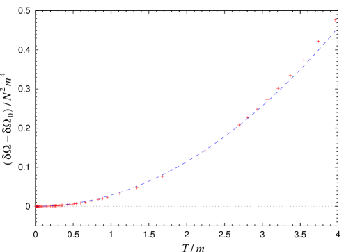
Figure 3: Numerical determination of the generalized free energy $\delta\Omega$ (6.71) with the leading behavior $\delta\Omega_{0}=-\pi^{2}N^{2}T^{4}/8$ subtracted. The numerical values are given by the data points, while the leading high-temperature correction, $\delta\Omega_{1}\equiv\Gamma(3/4)^{4}N^{2}m^{2}T^{2}/8\pi^{2}$, is indicated by the dashed line.

For a thermodynamic process at a fixed volume, the physical phase is realized from the minimization of the generalized free energy

$$\Omega[T,\mu]^{physical}=\min\left\{\Omega_{BH},\Omega_{PW}\right\}\,.$$ (6.73)

Thus the signature of a phase transition would be the vanishing of $\delta\Omega$ at a certain critical temperature $T_{c}$

$$\delta\Omega\left[T,\mu=-m/T\right]\bigg{|}_{T=T_{c}}=0\,.$$ (6.74)

In the high temperature phase, $m/T\ll 1$, we have found [compare with (6.66)]

$$\begin{split}\frac{\delta\Omega\left[T,-\frac{m}{T}\right]}{m^{4}N^{2}}\equiv&\frac{1}{m^{4}N^{2}}\biggl{(}\delta\Omega_{0}+\delta\Omega_{1}\biggr{)}+o\left(\frac{T^{2}}{m^{2}}\right)\\ =&-\frac{\pi^{2}}{8}\left(\frac{T}{m}\right)^{4}+\frac{\Gamma(3/4)^{4}}{8\pi^{2}}\left(\frac{T}{m}\right)^{2}+o\left(\frac{T^{2}}{m^{2}}\right)\,;\end{split}$$ (6.75)

that is, $\delta\Omega<0$. On the other hand, we have argued that in the low temperature phase, $m/T\gg 1$, we would instead expect $\delta\Omega>0$; see Fig. 1.

The result of the numerical work is shown in Fig. 3. While the numerics appear to be in good agreement with our analytical prediction (6.75), we have been unable to confirm the phase transition. One possibility is that the critical temperature of the conjectured phase transition is at $T_{c}=m\,\varrho$, where $\varrho$ is a small number. This would make numerical study of the transition rather challenging, as the ultra-low temperature supergravity flows (see Fig. 2) approach the supersymmetric (singular) PW flow, and are plagued by numerical instabilities. Another possibility is that in the large $N$ limit this phase transition is actually at $T_{c}=0$. This issue clearly deserves further investigation.

References

- [1] J. M. Maldacena, “The large limit of superconformal field theories and supergravity,” Adv. Theor. Math. Phys. 2, 231 (1998) [Int. J. Theor. Phys. 38, 1113 (1999)] [arXiv:hep-th/9711200].
- [2] O. Aharony, S. S. Gubser, J. M. Maldacena, H. Ooguri and Y. Oz, “Large field theories, string theory and gravity,” Phys. Rept. 323, 183 (2000) [arXiv:hep-th/9905111].
- [3] E. Witten, “Anti-de Sitter space, thermal phase transition, and confinement in gauge theories,” Adv. Theor. Math. Phys. 2, 505 (1998) [arXiv:hep-th/9803131].
- [4] A. Buchel, “Finite temperature resolution of the Klebanov-Tseytlin singularity,” Nucl. Phys. B 600, 219 (2001) [arXiv:hep-th/0011146].
- [5] S. S. Gubser, C. P. Herzog, I. R. Klebanov and A. A. Tseytlin, “Restoration of chiral symmetry: A supergravity perspective,” JHEP 0105 (2001) 028 [arXiv:hep-th/0102172].
- [6] A. Buchel and A. R. Frey, “Comments on supergravity dual of pure super Yang Mills theory with unbroken chiral symmetry,” Phys. Rev. D 64, 064007 (2001) [arXiv:hep-th/0103022].
- [7] S. S. Gubser, A. A. Tseytlin and M. S. Volkov, “Non-Abelian 4-d black holes, wrapped 5-branes, and their dual descriptions,” JHEP 0109, 017 (2001) [arXiv:hep-th/0108205].
- [8] S. W. Hawking and D. N. Page, “Thermodynamics Of Black Holes In Anti-de Sitter Space,” Commun. Math. Phys. 87,
- [9] I. R. Klebanov and A. A. Tseytlin, “Gravity duals of supersymmetric gauge theories,” Nucl. Phys. B 578, 123 (2000) [arXiv:hep-th/0002159].
- [10] I. R. Klebanov and M. J. Strassler, “Supergravity and a confining gauge theory: Duality cascades and chiSB-resolution of naked singularities,” JHEP 0008, 052 (2000) [arXiv:hep-th/0007191].
- [11] J. M. Maldacena and C. Nunez, “Towards the large limit of pure super Yang Mills,” Phys. Rev. Lett. 86, 588 (2001) [arXiv:hep-th/0008001].
- [12] A. Buchel, “On the thermodynamic instability of LST,” arXiv:hep-th/0107102.
- [13] K. Pilch and N. P. Warner, “ supersymmetric RG flows and the IIB dilaton,” Nucl. Phys. B 594, 209 (2001) [arXiv:hep-th/0004063].
- [14] A. Buchel, A. W. Peet and J. Polchinski, “Gauge dual and noncommutative extension of an supergravity solution,” Phys. Rev. D 63, 044009 (2001) [arXiv:hep-th/0008076].
- [15] N. Evans, C. V. Johnson and M. Petrini, “The enhancon and gauge theory/gravity RG flows,” JHEP 0010, 022 (2000) [arXiv:hep-th/0008081].
- [16] R. Donagi and E. Witten, “Supersymmetric Yang-Mills Theory And Integrable Systems,” Nucl. Phys. B 460, 299 (1996) [arXiv:hep-th/9510101].
- [17] C. P. Herzog, I. R. Klebanov and P. Ouyang, “D-branes on the conifold and gauge / gravity dualities,” arXiv:hep-th/0205100.
- [18] D. Z. Freedman and J. A. Minahan, “Finite temperature effects in the supergravity dual of the gauge theory,” JHEP 0101, 036 (2001) [arXiv:hep-th/0007250].
- [19] J. Polchinski and M. J. Strassler, “The string dual of a confining four-dimensional gauge theory,” arXiv:hep-th/0003136.
- [20] S. W. Hawking and G. T. Horowitz, “The Gravitational Hamiltonian, action, entropy and surface terms,” Class. Quant. Grav. 13, 1487 (1996) [arXiv:gr-qc/9501014].
- [21] M. Bianchi, D. Z. Freedman and K. Skenderis, “How to go with an RG flow,” JHEP 0108, 041 (2001) [arXiv:hep-th/0105276].
- [22] M. Bianchi, D. Z. Freedman and K. Skenderis, “Holographic renormalization,” Nucl. Phys. B 631, 159 (2002) [arXiv:hep-th/0112119].
- [23] G. Policastro, D. T. Son and A. O. Starinets, “From AdS/CFT correspondence to hydrodynamics,” JHEP 0209, 043 (2002) [arXiv:hep-th/0205052].
- [24] A. Buchel, “Comments on fractional instantons in gauge theories,” Phys. Lett. B 514, 417 (2001) [arXiv:hep-th/0101056].
- [25] S. S. Gubser, I. R. Klebanov and A. W. Peet, “Entropy and Temperature of Black 3-Branes,” Phys. Rev. D 54, 3915 (1996) [arXiv:hep-th/9602135].
- [26] J. H. Schwarz, “Covariant Field Equations of Chiral Supergravity,” Nucl. Phys. B226 (1983) 269.
- [27] A. Buchel, “Compactifications of the flow,” arXiv:hep-th/0302107.
- [28] Work in progress.