Witten’s Vertex Made Simple

Abstract

The infinite matrices in Witten’s vertex are easy to diagonalize. It just requires some $SL(2,\mathbb{R})$ lore plus a Watson-Sommerfeld transformation. We calculate the eigenvalues of all Neumann matrices for all scale dimensions $s$, both for matter and ghosts, including fractional $s$ which we use to regulate the difficult $s=0$ limit. We find that $s=1$ eigenfunctions just acquire a $p$ term, and $x$ gets replaced by the midpoint position.

I Introduction

Witten witten derived open strings from a field theory with cubic Lagrangian. Its loop graphs include closed strings freedman . The kinetic term is the BRST operator, which in Siegel gauge reduces to $c_{0}L_{0}$. Unfortunately the basis which diagonalizes $L_{0}$ leads to forbiddingly complicated formulae for the vertex GJ . It was known from the beginning that $K_{1}=L_{1}+L_{-1}$ commuted with Witten’s vertex, but only recently did Rastelli et al. spectroscopy have the idea of transforming it to the basis with $K_{1}$ diagonal. After a long indirect calculation, which omitted the momenta, they found that the Neumann matrices in the vertex take a simple diagonal form in this basis. The present paper has two aims. Firstly we develop a straightforward method for changing the basis. Secondly we resolve the momentum difficulties.

Here $L_{0}$, $L_{\pm 1}$ are the three generators of $SL(2,\mathbb{R})$. The world sheet fields in string theory belong to representations of this group, labelled by the scale dimension $s$ (also called the conformal weight). The string position $X^{\mu}(z)$ has $s=0$. If we omit the zero modes by applying $\frac{d}{dz}$, we get $s=1$. This was the case diagonalized by Rastelli et al. spectroscopy . String theory also uses $s=2,\,-1,\frac{1}{2},\frac{3}{2},-\frac{1}{2}$. $L_{0}$ has discrete eigenvalues $m+s$, which determine the mass spectrum of a free string. $K_{1}$ has continuous eigenvalues $\kappa$, but it is becoming clear that this basis is much more appropriate to interacting strings.

Going from one basis to the other is essentially a problem in $SL(2,\mathbb{R})$ representation theory. (However the $s=0$ limit is very singular.) In dealing with infinite dimensional representations it is important to be precise about the Hilbert space. Fortunately $SL(2,\mathbb{R})$ has been extensively studied by mathematicians bargmann ; gelfand ; ruhl . The appropriate Hilbert spaces for each $s$ consist of analytic functions $f(z)$ in the unit disk and they possess a Cauchy kernel — an integral operator $\mathrm{Id}_{s}(z,{\overline{z}}^{\prime})$ which represents the identity and projects onto the entire space. For any complete basis in the Hilbert space, this Cauchy kernel must be a sum of outer products of the basis functions, which fact can be used to normalize them. The Neumann matrices in Witten’s vertex are the matrix elements in the $L_{0}$ basis of other integral operators peskin1 , which we call Neumann kernels. Now each of these kernels is just a known function of two complex variables. All of them can be expanded in outer products of $K_{1}$ eigenfunctions by the Watson- Sommerfeld contour deformation trick (familiar to physicists old enough to remember Regge poles). As expected, they are all diagonal in this basis. Dividing the diagonalized Neumann kernels by the Cauchy kernel then normalizes the eigenfunctions and immediately gives the Neumann eigenvalues. No matrix calculations are needed - one just has to check the validity of the contour deformation.

This works for any scale dimension $s$, thus allowing us to use $s$ as a regulator for the singular $s=0$ limit. The exponent of the vertex contains a $\frac{1}{s}$ pole which enforces momentum conservation fubini . The situation in the $K_{1}$ basis is still complicated because overlapping singularities have to be disentangled. However we discovered a unitary transformation which separates them. Even better, it can be reinterpreted as a string field redefinition which removes the annoying nonlocality from Witten’s vertex, and which transforms the ghost zero mode $c_{0}$ into the kinetic term conjectured for the nonperturbative vacuum rastelli .

Rastelli et al.spectroscopy only considered $s=1$, but a number of subsequent authors marino ; arevefa ; dima1 ; Erler extended their method to the other cases needed in string theory. Our general proof is an order of magnitude shorter, but we confirm most of their conclusions. The exception is $s=0$, which is crucial. Our answer is simple: Including the momentum does nothing to the continuum eigenvalues. It adds a momentum term to their eigenfunctions, and also a zero mode oscillator which is just that for $L_{0}$ with $x$ replaced by the midpoint position $X_{L}(i)+X_{L}(-i)$. In view of the controversy about $s=0$, we checked in detail that we recover the correct Neumann matrix elements when we transform back to the $L_{0}$ basis.

In section II, we review $SL(2,\mathbb{R})$ representations for different scale dimensions $s$, and carefully normalize the eigenvectors $|m,s\rangle$ of $L_{0}$ and $|\kappa,s\rangle$ of $K_{1}$. In section III we diagonalize the $N$-string Neumann matrices for matter fields and in section VI the $3$-string matrices for the ghosts and superghosts, using Watson-Sommerfeld transformations. Each matrix is diagonalized independently, so the identities connecting them are a cross-check. In section IV we examine the zero modes closely. Most of the confusion in earlier papers arose from regularizing them inconsistently. Section V checks that the momentum Neumann matrices can be correctly reconstructed. Section VII is a summary. In Appendix A, we calculate $L_{0}$ in the new basis. Appendix B lists some lemmas.

II Normalized Eigenfunctions

II.1 Representations of $SL(2,\mathbb{R})$

It is well known that the group $SL(2,\mathbb{R})$ is isomorphic to the group $SU(1,1)$ of quasiunitary unimodular $2\times 2$ matrices $\Lambda=\begin{pmatrix}\alpha&\beta\\ \bar{\beta}&\bar{\alpha}\end{pmatrix}$ with $|\alpha|^{2}-|\beta|^{2}=1$. This is also known as a group of fractional linear transformations preserving the unit circle:

$$T_{\Lambda}(z)=\frac{\alpha z+\beta}{\bar{\beta}z+\bar{\alpha}}.$$ (2.1)

Its unitary representations were first considered by Bargmann bargmann . Good references are gelfand and ruhl . The important representations for string field theory are the discrete series $\mathscr{D}^{+}_{s}$, because they can be realized on analytic functions (Here $s$ is the scale dimension). The representations $\mathscr{D}^{+}_{s}$ are single valued only for $s=1,2,\dots$, while for half integer $s$ they represent the double covering group. Unitarity fails at $s=0$, but we can continue the representation using $s$ as a regulator. An appropriate Hilbert space $\mathcal{H}_{s}$ consists of functions $f(z)$ analytic inside the unit circle and square-integrable on the boundary. The inner product is given by ruhl

$$\langle g|f\rangle=\frac{1}{\pi\Gamma(2s-1)}\,\int_{|z|\leqslant 1}d^{2}z\,\bigl{[}1-z{\overline{z}}\bigr{]}^{2s-2}\,\overline{g(z)}f(z).$$ (2.2)

The apparent singularity at $s=\frac{1}{2}$ is spurious ruhl , but there is a real one at $s=0$. Note the two-dimensional integral. We need a well-behaved adjoint, so we do not use analytic conformal field theory.

The representation of the group (2.1) on this Hilbert space is of the form

$$(T_{\Lambda}f)(z)=(\bar{\beta}z+\bar{\alpha})^{-2s}\,f\left(\frac{\alpha z+\beta}{\bar{\beta}z+\bar{\alpha}}\right).$$ (2.3)

In other words $f(z)$ is a form of degree $s$: $f(z)(dz)^{s}$ is invariant under the transformation (2.1). One can easily check that the inner product (2.2) is invariant with respect to transformation (2.3), i.e. $\langle T_{\Lambda}g|T_{\Lambda}f\rangle=\langle g|f\rangle$. Hence $T_{\Lambda}$ represents a unitary operator on this Hilbert space.

The Virasoro generators are

$$L_{n}=z^{n+1}\frac{d}{dz}+(n+1)sz^{n}.$$ (2.4)

$SL(2,\mathbb{R})$ is generated by $L_{0},\,L_{\pm 1}$.

II.2 Bases in $\mathcal{H}_{s}$

II.2.1 The discrete basis

The usual basis diagonalizes the elliptic generator $L_{0}$, which has discrete eigenvalues $(m+s)$, $m=0,1,2,\dots$. Its eigenfunctions normalized by (2.2) are

$$|m,s\rangle(z)=N_{m}^{(s)}z^{m}\quad\text{with}\quad N_{m}^{(s)}=\left[\frac{\Gamma(m+2s)}{\Gamma(m+1)}\right]^{1/2}.$$ (2.5)

For $s=0,-\frac{1}{2},-1,\dots$, the first $1-2s$ normalization factors are singular. We can use fractional $s$ as a regulator, getting for example

$$|0,0\rangle(z)=(2s)^{-1/2}.$$

This point will be pursued in Section IV. The Casimir is $s(1-s)$, so there is a relation between the representations with $s$ and $1-s$, which is important for the ghosts. In particular,

$$N^{(1-s)}_{m+2s-1}\,N^{(s)}_{m}=1.$$ (2.6)

Also

$$\left(\frac{d}{dz}\right)^{2s-1}|m+2s-1,1-s\rangle(z)=|m,s\rangle(z).$$

Vectors on both sides of this equation are well defined for $s\geqslant\frac{1}{2}$ and $m\geqslant 0$.

II.2.2 The continuous basis

The generator $K_{1}=L_{1}+L_{-1}$ commutes with Witten’s star product witten , which therefore becomes simpler when it is diagonalized spectroscopy . It is convenient to map

$$z=i\tanh w,$$ (2.7)

which takes the unit disk into the strip $-\pi/4\leqslant\mathop{\textmd{Im}}\nolimits w\leqslant\pi/4$. We assume that under a map $z\mapsto w$ the vector $f(z)$ transforms in a trivial way

$$f(z)\mapsto f(z(w)).$$ (2.7^′)

Then

$$K_{1}=-i\frac{d}{dw}+2is\tanh w.$$ (2.8)

Since this is a hyperbolic generator, its eigenvalues are all real numbers $\kappa$. The eigenfunctions of (2.8) are

$$|\kappa,s\rangle(z)=\bigl{[}A_{s}(\kappa)\bigr{]}^{1/2}\,(\cosh w)^{2s}\,e^{i\kappa w},$$ (2.9)

where $A_{s}(\kappa)$ is an important normalization constant, which will be determined in Subsection II.2.4.

II.2.3 Transformation matrix between the discrete and continuous bases

Now we relate the two bases $|m,s\rangle(z)$ and $|\kappa,s\rangle(z)$ by expanding

$$(\cosh w)^{2s}\,e^{i\kappa w}=\sum_{m=0}^{\infty}V_{m}^{(s)}(\kappa)z^{m}.$$ (2.10)

The first two terms are easily calculated from (2.7): $V_{0}^{(s)}=1,\,V_{1}^{(s)}=\kappa$. By (2.4) the vectors $|\kappa,s\rangle(z)$ satisfy the equation

$$\left[(1+z^{2})\frac{d}{dz}+2sz-\kappa\right]|\kappa,s\rangle(z)=0.$$ (2.11)

This gives the recursion formula

$$V_{m}^{(s)}(\kappa)=\frac{1}{m}\left[\kappa\,V_{m-1}^{(s)}(\kappa)-(m+2s-2)\,V_{m-2}^{(s)}(\kappa)\right].$$ (2.12)

Thus the first five polynomials are

$$\begin{split}V_{0}^{(s)}&=1,\quad V_{1}^{(s)}=\kappa,\quad V_{2}^{(s)}=\frac{\kappa^{2}}{2}-s,\\ V_{3}^{(s)}&=\frac{\kappa^{3}}{6}-\Bigl{(}\frac{1}{3}+s\Bigr{)}\kappa,\\ V_{4}^{(s)}&=\frac{\kappa^{4}}{24}-\Bigl{(}\frac{1}{3}+\frac{s}{2}\Bigr{)}\kappa^{2}+\frac{s(s+1)}{2}.\end{split}$$ (2.13)

Some useful properties of the polynomials $V_{m}^{(s)}(\kappa)$ are listed in Appendix B. Normalizing both bases as in (2.9) and (2.5) gives the transformation matrix

$$\langle m,s|\kappa,s\rangle=V_{m}^{(s)}(\kappa)\,\frac{[A_{s}(\kappa)]^{\frac{1}{2}}}{N_{m}^{(s)}},$$ (2.14)

which is unitary for $s>0$. The unitarity follows from equation (B.2).

II.2.4 Normalization $A_{s}(\kappa)$

The normalization function $A_{s}(\kappa)$ has to be determined from

$$\langle\kappa^{\prime},s|\kappa,s\rangle=\delta(\kappa^{\prime}-\kappa).$$ (2.15)

Transforming (2.2) by (2.7) we obtain with $w=u+iv$

$$\langle g|f\rangle=\frac{1}{\pi\Gamma(2s-1)}\,\int_{-\infty}^{\infty}du\int_{-\pi/4}^{\pi/4}dv\,|\cosh w|^{-4s}\\ \times\bigl{[}\cos(2v)\bigr{]}^{2s-2}\,\overline{g(z(w))}f(z(w)).$$ (2.16)

Note that the $\cosh w$ factors cancel between (2.9) and (2.16), so conservation of $K_{1}$ is just translation invariance in $u$.

For $s=1$, the normalization $A_{s}$ in (2.9) can be easily obtained by direct calculation of the integral in (2.16):

$$A_{1}(\kappa)=\frac{\kappa}{2\sinh\frac{\pi\kappa}{2}}.$$ (2.17)

In other representations it is better to proceed indirectly. By (2.5)

$$\mathrm{Id}_{s}(z,{\overline{z}}^{\prime})=\sum_{m=0}^{\infty}|m,s\rangle(z)\otimes\langle m,s|(\overline{z}^{\prime})\\ =\Gamma(2s)\,\bigl{[}1-z\overline{z}^{\prime}\bigr{]}^{-2s},$$ (2.18)

where $\langle m,s|(\overline{z}^{\prime})\equiv\overline{|m,s\rangle(z^{\prime})}$. Mathematically this is the Cauchy kernel which projects onto the entire Hilbert space. Physically it is almost the propagator for scale dimension $s$. The divergent factor $\Gamma(2s)$ prevents it from becoming trivial for $s\to 0$. We can calculate $A_{s}(\kappa)$ by transforming (2.18) to the basis (2.9). Inserting $z=i\tanh w$ gives

$$\mathrm{Id}_{s}(z,{\overline{z}}^{\prime})=2^{2s}\,\Gamma(2s)\Bigl{[}\cosh w\cosh{\overline{w}}^{\prime}\Bigr{]}^{2s}\\ \times\Bigl{\{}e^{w-\overline{w}^{\prime}}+e^{\overline{w}^{\prime}-w}\Bigr{\}}^{-2s}.$$ (2.19)

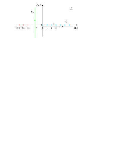
Figure 1: The dots represent the poles of the integrand in (2.20) or (3.18). Contour $C$ encircles the positive real axis counterclockwise. Then we deform it to contour $C_{-s}$, which lies parallel to the imaginary axis at $\mathop{\textmd{Re}}\nolimits j=-s$.

We perform a binomial expansion assuming $\mathop{\textmd{Re}}\nolimits(\overline{w}^{\prime}-w)<0$, and then rewrite it as a contour integral

$$\Bigl{\{}e^{w-\overline{w}^{\prime}}+e^{\overline{w}^{\prime}-w}\Bigr{\}}^{-2s}\\ =\sum_{j=0}^{\infty}\frac{\Gamma(2s+j)}{\Gamma(2s)\Gamma(j+1)}\,(-1)^{j}\,\left[e^{\overline{w}^{\prime}-w}\right]^{2(s+j)}\\ =\frac{1}{2i}\,\oint_{C}dj\,\frac{1}{\sin(\pi j)}\,\frac{\Gamma(2s+j)}{\Gamma(2s)\Gamma(j+1)}\,\left[e^{\overline{w}^{\prime}-w}\right]^{2(s+j)},$$ (2.20)

where the contour $C$ encircles the positive real axis counterclockwise (see Figure 1). Now we use the Watson-Sommerfeld trick of deforming the contour to lie parallel to the imaginary axis. As $\mathop{\textmd{Im}}\nolimits j\to\pm\infty$

$$\frac{1}{\sin(\pi j)}\sim e^{-\pi|\mathop{\textmd{Im}}\nolimits j|}\quad\text{and}\quad\frac{\Gamma(2s+j)}{\Gamma(2s)\Gamma(j+1)}\,\sim|j|^{2s-1},$$

so the integrand vanishes at infinity. Since $\Gamma(z+1)$ has poles at negative integers, the second factor in the integral (2.20) will have poles at $j=-2s-n$ ($n=0,1,2,\dots$) and zeros at $j=-1,-2,\dots$. These zeros will cancel the poles of $\bigl{[}\sin(\pi j)\bigr{]}^{-1}$ at negative integers. So for $s>0$ we can deform the contour to $\mathop{\textmd{Re}}\nolimits j=-s$ without meeting any poles (see Figure 1). However as $s\to 0$ the poles at $j=0$ and $j=-2s$ will coincide, pinching the contour between them. Since the real axis was encircled counterclockwise, the new integral will go down the imaginary axis. Therefore we write

$$j=-s-\frac{i\kappa}{2},$$ (2.21)

obtaining finally

$$\mathrm{Id}_{s}(z,{\overline{z}}^{\prime})=\int_{-\infty}^{\infty}d\kappa\,A_{s}(\kappa)\,\bigl{[}\cosh w\cosh{\overline{w}}^{\prime}\bigr{]}^{2s}\\ \times e^{i\kappa(w-\overline{w}^{\prime})}\equiv\int_{-\infty}^{\infty}d\kappa\,|\kappa,s\rangle(z)\otimes\langle\kappa,s|({\overline{z}}^{\prime})$$ (2.22)

with

$$A_{s}(\kappa)=\frac{2^{2s-2}}{\pi}\,\Gamma\Bigl{(}s+\frac{i\kappa}{2}\Bigr{)}\Gamma\Bigl{(}s-\frac{i\kappa}{2}\Bigr{)}.$$ (2.23)

Using relations among $\Gamma$-functions one can easily obtain the following recurrence formula:

$$A_{s}(\kappa)=\frac{A_{s+1}(\kappa)}{\kappa^{2}+4s^{2}}.$$ (2.24)

By (2.14), $V_{m}^{(s)}(\kappa)$ are orthogonal polynomials with weight $A_{s}(\kappa)$. The orthogonality formula (B.2) is easily checked from (B.1), which is a standard Fourier transform.

Special cases of equation (2.23) are

$$A_{1}(\kappa) =\frac{\kappa}{2\sinh\frac{\pi\kappa}{2}}$$ (2.25a)

which agrees with (2.17) and the result of okuyama1 ,

$$A_{\frac{1}{2}}(\kappa) =\frac{1}{2\cosh\frac{\pi\kappa}{2}}$$ (2.25b)

which agrees with arevefa , and especially

$$A_{0}(\kappa) =\lim_{s\to+0}\frac{A_{s+1}(\kappa)}{\kappa^{2}+4s^{2}},$$ (2.25c)

which requires some explanation. We did not evaluate the limit $s\to 0$ because the expressions multiplying $A_{0}(\kappa)$ may depend on $s$, and therefore the limit can change. Some of the following expressions will be used in our calculations:

$$\lim_{s\to+0}\frac{\kappa}{\kappa^{2}+4s^{2}}=\mathscr{P}\frac{1}{\kappa},\quad\lim_{s\to+0}\frac{2s}{\kappa^{2}+4s^{2}}=\pi\,\delta(\kappa)\\ \quad\text{and}\quad\lim_{s\to+0}\frac{s^{m}}{\kappa^{2}+4s^{2}}=0,\quad m\geqslant 2.$$ (2.26)

An example of the use of these expressions is (B.4). In the expression for the eigenvector (2.9) we use the square root of $A_{s}$, and hence we need to know the limit $\sqrt{A_{s}(\kappa)}$ as $s\to 0$. At this point it is necessary to include the sign of $\kappa$ in the definition of $\sqrt{A_{0}(\kappa)}$, so that

$$\sqrt{A_{0}(\kappa)}=\lim_{s\to 0}\frac{\mathop{\mathrm{sgn}}\nolimits(\kappa)}{\sqrt{\kappa^{2}+4s^{2}}}\,\sqrt{A_{s+1}(\kappa)}\\ \equiv\mathscr{P}\,\frac{\sqrt{A_{1}(\kappa)}}{\kappa}.$$ (2.27)

It follows from (B.3), (2.14) and (2.24) that

$$\langle m+1,0|\kappa,0\rangle=\langle m,1|\kappa,1\rangle,$$ (2.28)

so $s=1$ is just $s=0$ with $m=0$ omitted.

Equation (2.26) means that for $s=0$ the spectrum of $K_{1}$ includes an additional $\kappa=0$ eigenstate superimposed on the continuum. This will be discussed further in Section IV. (2.28) also means that $s=0$ adds an $m=0$ border to $s=1$.

The ghosts and superghosts appear in the tensor product of the representations $\mathscr{D}_{s}^{+}$ and $\mathscr{D}_{1-s}^{+}$. From equation (2.23) one gets

$$\bigl{(}A_{n}A_{1-n}\bigr{)}^{1/2} =\frac{1}{2\sinh\frac{\pi\kappa}{2}},$$ (2.29a)

$$\bigl{(}A_{n+\frac{1}{2}}A_{\frac{1}{2}-n}\bigr{)}^{1/2} =\frac{1}{2\cosh\frac{\pi\kappa}{2}}\equiv A_{\frac{1}{2}}(\kappa).$$ (2.29b)

III Matter Vertex

III.1 Review of the gluing vertices

III.1.1 Oscillator normalization

Consider a primary conformal field $\mathcal{O}_{s}(z)$ of dimension $s$. Here we assume that $2s$ is an integer, and $\mathcal{O}_{s}(z)$ is a boson or fermion depending on whether $s$ is an integer or half integer. In the $NS$ sector the field has a mode expansion

$$\mathcal{O}_{s}(z)=\sum_{m\in\mathbb{Z}-s}\frac{\mathcal{O}_{m}}{z^{m+s}}.$$ (3.1)

We decompose it into creation and annihilation parts with respect to the $SL(2,\mathbb{R})$-invariant vacuum:

$$\mathcal{O}_{s}(z)=\sum_{n=0}^{\infty}N_{n}^{(s)}\Bigl{[}\mathbf{a}_{n}^{+}\,z^{n}+\mathbf{a}_{n}^{-}\,z^{-n-2s}\Bigr{]}+\text{rest},$$ (3.2)

where $N_{n}^{(s)}$ is defined by (2.5), and

$$N_{n}^{(s)}\,\mathbf{a}^{\pm}_{n}=\mathcal{O}_{\mp(n+s)}.$$ (3.3a)

The “rest” consists of oscillators annihilating both the $$SL(2,\mathbb{R}) s=1 p/z$$-invariant vacuum and its conjugate (for example for it contains ). We assume the following (anti)commutation relations between the oscillators

$$[\mathbf{a}_{n}^{-},\,\mathbf{a}^{+}_{m}]_{\pm}=\delta_{nm}.$$ (3.3b)

Although these are not the most general commutation relations, they cover the cases in which we are interested: bosonic fields with $s=0$ or $s=1$ and fermionic field with $s=\frac{1}{2}$. In any case the two point correlation function of fields $\mathcal{O}_{s}(z)$ on the plane is

$$\langle\mathcal{O}_{s}(z)\mathcal{O}_{s}(z^{\prime})\rangle=\frac{\Gamma(2s)}{(z-z^{\prime})^{2s}},$$ (3.4)

where $\Gamma(2s)$ comes from our normalization convention (3.3b).

Before we proceed with formulation of a gluing vertex let us consider a couple of examples: $s=1$ and $s=\frac{1}{2}$. Discussion of the tricky case $s=0$ we postpone to Section IV.

For $s=\frac{1}{2}$ the fermionic conformal field $\psi(z)$ has the following mode expansion GSW

$$\psi(z)=i\left[\frac{\alpha^{\prime}}{2}\right]^{\frac{1}{2}}\,\sum_{m\in\mathbb{Z}+\frac{1}{2}}\frac{\psi_{m}}{z^{m+\frac{1}{2}}}$$ (3.5a)

and the two point correlation function on the plane is

$$\langle\psi(z)\psi(z^{\prime})\rangle=-\frac{\alpha^{\prime}}{2}\,\frac{1}{z-z^{\prime}}.$$ (3.5b)

By comparing this correlation function with (3.4) for $$s=\frac{1}{2}$$ one concludes that

$$i\left[\frac{\alpha^{\prime}}{2}\right]^{\frac{1}{2}}\,\mathcal{O}_{\frac{1}{2}}(z)=\psi(z),$$

and therefore

$$\quad\mathbf{a}_{n}^{\pm}=\psi_{\mp(n+\frac{1}{2})},\quad n\geqslant 0.$$ (3.5c)

For $s=1$ the bosonic conformal field $\partial X(z)$ has the following mode expansion GSW

$$i\partial X(z)=\left[\frac{\alpha^{\prime}}{2}\right]^{\frac{1}{2}}\,\sum_{m\in\mathbb{Z}}\frac{\alpha_{m}}{z^{m+1}}$$ (3.6a)

and the two point correlation function on the plane is

$$\langle\partial X(z)\partial X(z^{\prime})\rangle=-\frac{\alpha^{\prime}}{2}\,\frac{1}{(z-z^{\prime})^{2}}.$$ (3.6b)

By comparing this correlation function with (3.4) for $$s=1$$ one concludes that

$$\left[\frac{\alpha^{\prime}}{2}\right]^{\frac{1}{2}}\,\mathcal{O}_{1}(z)=i\partial X(z),$$

and therefore

$$\mathbf{a}_{n}^{\pm}=\frac{\alpha_{\mp(n+1)}}{\sqrt{n+1}},\quad n\geqslant 0.$$ (3.6c)

III.1.2 Continuum oscillators

So by the unitary transformation (2.14),

$$\mathbf{a}^{\pm}(\kappa)=\sqrt{A_{s}(\kappa)}\,\sum_{m=0}^{\infty}\frac{V_{m}^{(s)}(\kappa)}{N_{m}^{(s)}}\,\mathbf{a}_{m}^{\pm}$$ (3.7)

are the oscillators in the $\kappa$-basis, satisfying

$$[\mathbf{a}^{-}(\kappa),\,\mathbf{a}^{+}(\kappa^{\prime})]_{\pm}=\delta(\kappa-\kappa^{\prime}).$$ (3.8)

Now we expand world sheet fields $\mathcal{O}_{s}(z)$ in these $\kappa$-oscillators. We assume that $z$ is on the unit circle, which allows us to change $1/z$ to ${\overline{z}}$ (This is not a restriction for us, because we are only interested in the world-sheet fields on the boundary). Hence the expansion is

$$\left.\mathcal{O}_{s}(z)\right|_{|z|=1}=\int_{-\infty}^{\infty}d\kappa\,\Bigl{\{}\mathbf{a}^{+}(\kappa)\,|\kappa,s\rangle(z)+\mathbf{a}^{-}(\kappa)\,{\overline{z}}^{2s}\,|\kappa,s\rangle({\overline{z}})\Bigr{\}}+\text{rest}\\ \equiv\int_{-\infty}^{\infty}d\kappa\,\sqrt{A_{s}(\kappa)}\,\Bigl{\{}\mathbf{a}^{+}(\kappa)\,[\cosh w]^{2s}\,e^{i\kappa w}+\mathbf{a}^{-}(\kappa)\,{\overline{z}}^{2s}\,[\cosh{\overline{w}}]^{2s}\,e^{-i\kappa{\overline{w}}}\Bigr{\}}+\text{rest}.$$ (3.9)

This expansion is easy to obtain by using the representation (2.22) for the Cauchy kernel.

III.1.3 Gluing vertex

The $N$-string vertex $\langle V^{(s)}_{N}|$ is a multilinear map from the $N$-th power of an oscillator Fock space to the complex numbers. For a conformal field $\mathcal{O}_{s}(z)$ of dimension $s$ (described in subsection III.1.1) it can be written as a Gaussian state of the form

$$\langle V^{(s)}_{N}|={}_{1\dots N}\langle 0|\exp\left[\frac{(-1)^{2s}}{2}\sum_{n,m=0}^{\infty}\sum_{I,J=1}^{N}\bigl{(}M_{s,N}^{IJ}C\bigr{)}_{mn}\,\mathbf{a}_{m}^{-(I)}\mathbf{a}_{n}^{-(J)}\right].$$ (3.10)

Here ${}_{1\dots N}\langle 0|$ is a tensor product of $SL(2,\mathbb{R})$ invariant vacua from each Fock space, $\mathbf{a}_{n}^{-(I)}$ are annihilation oscillators (3.3b) acting in the $I$-th Fock space, $C_{nm}=(-1)^{n}\delta_{nm}$ is a twist matrix and $M_{s,N,\,\,nm}^{IJ}$ are the Neumann matrices defining the gluing vertex GJ ; peskin1 . The Neumann matrices are symmetric or skewsymmetric $\bigl{(}M_{s,N}^{IJ}C\bigr{)}_{mn}=(-1)^{2s}\bigl{(}M_{s,N}^{JI}C\bigr{)}_{nm}$ and satisfy the cyclicity property $M_{s,N}^{IJ}=M_{s,N}^{I+1,J+1}$.

For any string field theory matter vertex, the Neumann matrices can be generated from a kernel operator

$$\begin{split}\bigl{(}M_{s,N}^{IJ}C\bigr{)}_{mn}&=\langle m,s|M_{s,N}^{IJ}C|n,s\rangle,\\ \bigl{(}M_{s,N}^{IJ}\bigr{)}_{mn}&=\langle m,s|M_{s,N}^{IJ}|n,s\rangle,\end{split}$$ (3.11)

where the states are (2.5). The expression for the operator $M_{s,N}^{IJ}C$ can by obtained using the conformal definition peskin1 of the gluing vertex:

$$\bigl{(}M_{s,N}^{IJ}C\bigr{)}(z,{\overline{z}}^{\prime})=\Gamma(2s)\,\\ \times\left\{\frac{\Bigl{[}h_{I}^{\prime}(z)\Bigr{]}^{s}\Bigl{[}h_{J}^{\prime}({\overline{z}}^{\prime})\Bigr{]}^{s}}{\Bigl{[}h_{I}(z)-h_{J}({\overline{z}}^{\prime})\Bigr{]}^{2s}}-\frac{\delta^{IJ}}{(z-{\overline{z}}^{\prime})^{2s}}\right\},$$ (3.12)

where $I,J=1,\dots,N$ label the glued strings and the maps $h_{I}(z)$ are defined below. Essentially (3.12) just generalizes LeClair et al. peskin1 to arbitrary scale dimension $s$. The powers of $s$ are determined by covariance under (2.3). The denominator must match the propagator (3.4). When $s$ is fractional we assume the principal branch of the power function, in other words the branch cut is on the negative real axis. The $\Gamma$-function is needed to give a nontrivial $s\to 0$ limit. To be consistent with our scalar product (2.2) we have put ${\overline{z}}^{\prime}$ as the second argument instead of $z^{\prime}$. The second term proportional to $(z-{\overline{z}}^{\prime})^{-2s}$ comes from the normal ordering when one acts by two operators of weight $s$ in the same Fock space. When using a contour integral representation for the Neumann matrices (as in peskin1 ) one never sees this term: it simply gives zero contribution. In our calculations this term cancels some divergences appearing in the diagonalization of $M^{II}_{s,N}$. Gross and Jevicki GJ (paper 3, eq. (3.28)) also mentioned that the free propagator must be subtracted from $M^{II}_{s,N}$.

Projecting with (2.5) in (3.11) is equivalent to expanding (3.12) in $z$ and ${\overline{z}}^{\prime}$, picking out the term $z^{m}{\overline{z}}^{\prime\,n}$ and then dividing its coefficient by $N_{m}^{(s)}N_{n}^{(s)}$. (This last assumes oscillators are normalized $[\mathbf{a}_{m}^{-},\,\mathbf{a}_{n}^{+}]=\delta_{mn}$.) The contour integrals in peskin1 achieve the same result.

To obtain an expression for the operator $M_{s,N}^{IJ}$ it is enough to notice that the twist operator $C$ acts on the eigenvectors $|n,s\rangle(z)$ by changing the sign of the argument $z$:

$$\bigl{(}C|n,s\rangle\bigr{)}(z)=|n,s\rangle(-z).$$ (3.13)

In other words to get an expression for $M_{s}^{IJ}$ one has just to change the sign of ${\overline{z}}$ in (3.12):

$$M_{s,N}^{IJ}(z,{\overline{z}}^{\prime})=\Gamma(2s)\,\\ \times\left\{\frac{\Bigl{[}h_{I}^{\prime}(z)\Bigr{]}^{s}\Bigl{[}h_{J}^{\prime}(-{\overline{z}}^{\prime})\Bigr{]}^{s}}{\Bigl{[}h_{I}(z)-h_{J}(-{\overline{z}}^{\prime})\Bigr{]}^{2s}}-\frac{\delta^{IJ}}{(z+{\overline{z}}^{\prime})^{2s}}\right\}$$ (3.14)

III.2 Diagonalizing Witten’s vertices

Different string field theories use different maps $h_{I}(z)$. For Witten’s $3$-string vertex

$$h_{2}(z)=\left(\frac{1-iz}{1+iz}\right)^{2/3}=e^{4w/3},$$ (3.15a)

where $$z=i\tanh w$$, and

$$h_{1,3}(z)=e^{\pm 2\pi i/3}\,h_{2}(z).$$ (3.15b)

However we can diagonalize the $N$-string vertex for very little extra trouble. We therefore take

$$h_{I}(z)=e^{i\varphi_{I}}\left(\frac{1-iz}{1+iz}\right)^{2/N}=e^{i\varphi_{I}}\,e^{4w/N},$$ (3.16)

where $z=i\tanh w$ and $\varphi_{I}=\frac{2\pi}{N}\,(\alpha_{N}-I)$. Here $\alpha_{N}$ is a real number which is chosen in such a way that all angles $\varphi_{I}$ lie in the range $(-\pi,\pi]$. This last requirement is important because we use rational powers in the definition of the Neumann matrix. Then

$$h_{I}^{\prime}(z)=-\frac{4i}{N}\,\cosh^{2}w\,h_{I}(z).$$ (3.17)

As we saw in (2.16) the map $z\to w$ takes the unit disk into the strip $-\pi/4\leqslant\mathop{\textmd{Im}}\nolimits w\leqslant\pi/4$. The maps $w\to h_{I}$ then transform this strip into $N$ $360^{o}/N$ wedges, which are glued together by the Neumann matrices peskin1 . Note that (3.14) is homogeneous in the $h_{I}$’s. The $\cosh w$ factors from (3.17) and (2.9) always cancel against the inner product (2.16), so homogeneity in $h$ implies translation invariance under $w\to w+c$, $\overline{w}^{\prime}\to\overline{w}^{\prime}+c$, and therefore conservation of $K_{1}$.

To diagonalize the $N$-string Neumann matrix, we proceed as in (2.19) et seq. — first a binomial expansion of (3.14), then a Watson-Sommerfeld transformation. The final result is the same whichever way round one does the binomial expansion. Thus if $\mathop{\textmd{Re}}\nolimits(\overline{w}^{\prime}-w)<0$,

$$M^{IJ}_{s,N}(z,{\overline{z}}^{\prime})=\Bigl{[}\cosh w\cosh\overline{w}^{\prime}\Bigr{]}^{2s}\!\oint_{C}\frac{dj}{2i\sin(\pi j)}\frac{\Gamma(2s+j)}{\Gamma(j+1)}\\ \times\Biggl{\{}\left(\frac{4}{N}\right)^{2s}\left[-e^{i(\varphi_{J}-\varphi_{I})}e^{4(\overline{w}^{\prime}-w)/N}\right]^{s+j}-\delta^{IJ}\,2^{2s}\left[-e^{2(\overline{w}^{\prime}-w)}\right]^{s+j}\Biggr{\}},$$ (3.18)

where $\varphi_{J}-\varphi_{I}=\frac{2\pi}{N}\,(I-J)$. The contour $C$ encircles the positive real axis counterclockwise (see Figure 1). Before deforming it as in Figure 1 we must worry about the contour at infinity. Starting from here we will consider $I\neq J$ and $I=J$ separately.

III.3 Matrices $M_{s,N}^{IJ}$ for $I\neq J$

By cyclic symmetry we can fix $I=1$, then $J=2,\dots,N$. In this case we can interpret $(-1)=e^{i\pi}$ and therefore

$$-e^{i(\varphi_{J}-\varphi_{1})}=e^{\frac{2\pi i}{N}\left(1-J+\frac{N}{2}\right)}.$$

This guarantees that for $2\leqslant J\leqslant N$

$$-\pi<\arg\Bigl{(}-e^{i(\varphi_{J}-\varphi_{1})}\Bigr{)}<\pi.$$ (3.19)

After dividing by $\sin(\pi j)$ we get the following asymptotic behavior of the integrand

$$\sim|j|^{2s-1}\,e^{-2\pi|\mathop{\textmd{Im}}\nolimits j|/N}$$

as $\mathop{\textmd{Im}}\nolimits j\to\pm\infty$. Hence for $M^{1J}$ ($J\neq 1$) the integrand vanishes at infinity. The poles of $\bigl{[}\sin(\pi j)\bigr{]}^{-1}$ at negative integers are cancelled by zeros of $\bigl{[}\Gamma(j+1)\bigr{]}^{-1}$, so for $s>0$ we can shift the contour to $\mathop{\textmd{Re}}\nolimits j=-s$ as in Figure 1 by writing

$$j=-s-\frac{iN\kappa}{4}$$ (3.20)

to get

$$M^{1J}_{s,N}(z,{\overline{z}}^{\prime})=\int_{-\infty}^{\infty}d\kappa\,e^{\frac{\pi\kappa}{4}\,(2+N-2J)}\,B_{s,N}(\kappa)\,\\ \times e^{i\kappa(w-\bar{w}^{\prime})}\,\bigl{(}\cosh w\cosh\overline{w}^{\prime}\bigr{)}^{2s},$$ (3.21)

where

$$B_{s,N}(\kappa)=\frac{1}{2\pi}\left[\frac{4}{N}\right]^{2s-1}\Gamma\Bigl{(}s+\frac{iN\kappa}{4}\Bigr{)}\Gamma\Bigl{(}s-\frac{iN\kappa}{4}\Bigr{)}.$$ (3.22)

This displays the Neumann matrix as an outer product of $K_{1}$ eigenfunctions (2.9). Notice also that the normalization $A_{s}(\kappa)$ introduced in (2.23) is equal to $B_{s,2}(\kappa)$.

III.4 Matrix $M^{II}_{s,N}$

If $I=J$, the first term in (3.18) contains a factor

$$(-1)^{s+j}=e^{\pm i\pi(s+j)}.$$

Either interpretation of $(-1)$ will cancel the nice falloff of $\bigl{[}\sin(\pi j)\bigr{]}^{-1}$ in (3.18) and prevent deformation of the contour. However in this case the second term in (3.18) comes into play. The bad asymptotic behavior at $\mathop{\textmd{Im}}\nolimits j\to\pm\infty$ is closely related to the coincident singularity at $w={\overline{w}}^{\prime}$ coming from the vanishing denominators in (3.14). Thus

$$\sim\rho^{2s}\,\int^{i\infty}dj\,j^{2s-1}\,\left[e^{\rho(\overline{w}^{\prime}-w)}\right]^{j}\sim(w-\overline{w}^{\prime})^{-2s},$$

where $\rho=4/N$ for the first term in (3.18) and $\rho=2$ for the second one. Therefore the singularity at $\mathop{\textmd{Im}}\nolimits j=\pm\infty$ cancels between these terms and we can deform the contour as in Figure 1.

Notice that the second term in (3.18) differs from the identity kernel (2.20) only by the the factor $(-1)^{s+j}$. Therefore deformation of $j$ as in (3.20) for the first term and as in (2.21) for the second term yields

$$M_{s,N}^{11}(z,{\overline{z}}^{\prime})=\int_{-\infty}^{\infty}d\kappa\,e^{i\kappa(w-{\overline{w}}^{\prime})}\,\bigl{(}\cosh w\cosh\overline{w}^{\prime}\bigr{)}^{2s}\\ \times\Bigl{\{}e^{\pm\pi\kappa N/4}B_{s,N}(\kappa)-e^{\pm\pi\kappa/2}A_{s}(\kappa)\Bigr{\}},$$ (3.23)

where $B_{s,N}(\kappa)$ is (3.22) and $A_{s}(\kappa)$ is (2.23). The asymptotic behavior is

$$\sim\frac{e^{\pm N\pi\kappa/4}}{e^{N\pi|\kappa|/4}}-\frac{e^{\pm\pi\kappa/2}}{e^{\pi|\kappa|/2}},$$ (3.24)

so the contour at infinity cancels if we choose the same sign in both terms.

III.5 Summary

Here we present the results of the calculations performed in this section. First we list the eigenvalues of operators (3.14) for general $N$ and discuss their properties. Second we present the results for $N=3$ and certain values of $s$.

III.5.1 $N$-string Neumann eigenvalues

The eigenfunctions have to be normalized by dividing by $A_{s}(\kappa)$ from (2.23), so the Neumann eigenvalues are

$$\mu^{II}_{s,N}(\kappa) =e^{\pm\pi\kappa N/4}\frac{B_{s,N}(\kappa)}{A_{s}(\kappa)}-e^{\pm\pi\kappa/2},$$ (3.25a)

$$\mu^{IJ}_{s,N}(\kappa) =e^{+\frac{\pi\kappa}{4}\,(N+2I-2J)}\,\frac{B_{s,N}(\kappa)}{A_{s}(\kappa)}\quad(I<J),$$ (3.25b)

$$\mu^{IJ}_{s,N}(\kappa) =(-1)^{2s}e^{-\frac{\pi\kappa}{4}\,(N-2I+2J)}\,\frac{B_{s,N}(\kappa)}{A_{s}(\kappa)}\quad(I>J),$$ (3.25c)

​​​where $(-1)^{2s}$ reflects the symmetry or skewsymmetry of the Neumann matrices ($\mu^{JI}_{s,N}(\kappa)=(-1)^{2s}\mu^{IJ}_{s,N}(-\kappa)$), and

$$\frac{B_{s,N}(\kappa)}{A_{s}(\kappa)}=\left[\frac{2}{N}\right]^{2s-1}\,\frac{\Gamma\Bigl{(}s+\frac{iN\kappa}{4}\Bigr{)}\Gamma\Bigl{(}s-\frac{iN\kappa}{4}\Bigr{)}}{\Gamma\Bigl{(}s+\frac{i\kappa}{2}\Bigr{)}\Gamma\Bigl{(}s-\frac{i\kappa}{2}\Bigr{)}}.$$ (3.26)

The sign in (3.25a) is undetermined. For $s=0,1$ it makes no difference. For $s=\frac{1}{2}$ the “$+$” sign agrees with other authors. From (3.26) one easily obtains the recurrence formula relating eigenvalues for $s$ and $s+1$:

$$\frac{B_{s,N}(\kappa)}{A_{s}(\kappa)}=\frac{B_{s+1,N}(\kappa)}{A_{s+1}(\kappa)}\,\frac{\kappa^{2}+4s^{2}}{\kappa^{2}+\frac{16}{N^{2}}s^{2}}.$$ (3.27)

First, this shows that $B_{s}(\kappa)/A_{s}(\kappa)$ is not a continuous function at the point $(s,\kappa)=(0,0)$:

$$\lim_{s\to 0}\frac{B_{s,N}(0)}{A_{s}(0)}=\frac{N}{2}\quad\text{while}\quad\lim_{\kappa\to 0}\frac{B_{0,N}(\kappa)}{A_{0}(\kappa)}=\frac{2}{N}.$$ (3.28)

This discontinuity will be important in Section IV, when we will analyze the spectrum of $s=0$ Neumann matrices. Second, from equation (3.27) it follows that if we first take the limit $s\to 0$ then the continuous eigenvalues (3.25) for $s=0$ and $s=1$ coincide dima1 .

For $2s=\text{integer}$, the products of $\Gamma$-functions reduce to hyperbolic ones. In this case (3.26) takes the following form

$$\frac{B_{1,N}(\kappa)}{A_{1}(\kappa)}=\frac{\sinh\frac{\pi\kappa}{2}}{\sinh\frac{N\pi\kappa}{4}}=\frac{B_{0,N}(\kappa)}{A_{0}(\kappa)}$$ (3.29)

for $s=1$ or $s=0$ and

$$\frac{B_{\frac{1}{2},N}(\kappa)}{A_{\frac{1}{2}}(\kappa)}=\frac{\cosh\frac{\pi\kappa}{2}}{\cosh\frac{N\pi\kappa}{4}}.$$ (3.30)

for $s=\frac{1}{2}$.

III.5.2 Sliver and identity Neumann eigenvalues

From (3.25a) one can easily get the eigenvalue for the sliver Neumann matrix rastelli ; okuyama1

$$\Xi_{1}(\kappa)=\lim_{N\to\infty}\mu_{1,N}^{11}(\kappa)\\ =\lim_{N\to\infty}\left[\frac{\sinh\frac{\pi\kappa}{2}}{\sinh\frac{\pi N\kappa}{4}}\,e^{\frac{\pi N\kappa}{4}}-e^{\frac{\pi\kappa}{2}}\right]=-e^{-\frac{\pi|\kappa|}{2}}.$$ (3.31a)

Actually one can do even better. By (3.25a)

$$\Xi_{s}(\kappa)=\lim_{N\to\infty}\mu_{s,N}^{11}(\kappa)=\theta(\pm\kappa)\,\frac{|\kappa|^{2s-1}}{A_{s}(\kappa)}-e^{\pm\frac{\pi\kappa}{2}}.$$ (3.31b)

For $$s=\frac{1}{2}$$ one obtains

$$\Xi_{\frac{1}{2}}(\kappa)=\pm\mathop{\mathrm{sgn}}\nolimits(\kappa)\,e^{-\frac{\pi|\kappa|}{2}},$$ (3.31c)

which agrees with arevefa (equation (3.22)) if we choose the “$+$” sign in (3.25a).

The identity state is a surface state (3.10) determined by the map (3.16) for $N=1$. In our notation it is $\langle V_{1}|$. Hence it can be represented as an exponential of a quadratic form, which is defined by (3.14) for $N=1$. We will denote $M_{s,N=1}\equiv\mathcal{I}_{s}$. The spectrum of the operator $\mathcal{I}_{s}(z,{\overline{z}}^{\prime})$ can be determined from the general formula (3.25). For the special cases $s=0,1$ and $\frac{1}{2}$ it is

$$\mathcal{I}_{0}(\kappa)=\mathcal{I}_{1}(\kappa)=1\quad\text{and}\quad\mathcal{I}_{\frac{1}{2}}(\kappa)=\mp\tanh\frac{\pi\kappa}{4}.$$ (3.32)

The spectrum of the identity state for $s=\frac{1}{2}$ agrees with that found in arevefa (equation (3.21)) if we choose the upper “$-$” sign.

III.5.3 $3$-string Neumann eigenvalues

Finally we specialize to $N=3$, abbreviating

$$\textsl{x}\equiv\frac{\pi\kappa}{4}.$$ (3.33)

In the following formulae we suppress the index $N=3$ in $M^{IJ}_{s,N}$. Then for $s=1$ or $s=0$,

$$\begin{split}\mu_{1,0}^{II}(\kappa)&=-\frac{\sinh\textsl{x}}{\sinh 3\textsl{x}},\\ \mu_{1,0}^{I,I+1}(\kappa)&=e^{+\textsl{x}}\,\frac{\sinh 2\textsl{x}}{\sinh 3\textsl{x}},\\ \mu_{1,0}^{I+1,I}(\kappa)&=e^{-\textsl{x}}\,\frac{\sinh 2\textsl{x}}{\sinh 3\textsl{x}};\end{split}$$ (3.34a)

and for $$s=\frac{1}{2}$$

$$\begin{split}\mu_{\frac{1}{2}}^{II}(\kappa)&=\pm\frac{\sinh\textsl{x}}{\cosh 3\textsl{x}},\\ \mu_{\frac{1}{2}}^{I,I+1}(\kappa)&=+e^{+\textsl{x}}\,\frac{\cosh 2\textsl{x}}{\cosh 3\textsl{x}},\\ \mu_{\frac{1}{2}}^{I+1,I}(\kappa)&=-e^{-\textsl{x}}\,\frac{\cosh 2\textsl{x}}{\cosh 3\textsl{x}}.\end{split}$$ (3.34b)

For $s=1$, (3.34a) exactly coincides with Rastelli et al. spectroscopy . The sign ambiguity in (3.25a) cancels for $s=1,0$ but not for $s=\frac{1}{2}$. For $s=\frac{1}{2}$, $\mu^{IJ}_{\frac{1}{2}}(\kappa)$ in (3.34b) agrees with Marino and Schiappa marino if we choose the upper “$+$” sign.

For $s=0$ the continuous eigenvalues are the same as for the case $s=1$. This is in agreement with previous authors dima1 . The improvement here is that we have much simpler expressions for the eigenvectors as compared to dima1 .

In Section IV we will consider the zero modes more carefully. The continuum eigenvalues are indeed identical for $s=0$ and $s=1$. However there is an additional discrete state at $\kappa=0$ whose function is to replace the average position $x$ by the midpoint position.

IV Zero modes, $s\to 0$ limit

IV.1 The $L_{0}$ basis

The correct procedure for regularizing zero modes goes back to the earliest days of string theory fubini . First note that for $s\approx 0$, (2.18) becomes

$$\frac{1}{2s}-\log\bigl{(}1-z{\overline{z}}^{\prime}\bigr{)}=\frac{1}{2s}+\sum_{m=1}^{\infty}\frac{(z{\overline{z}}^{\prime})^{m}}{m}.$$

The divergence implements momentum conservation

$$\exp\left[-\frac{1}{2s}\sum_{I,J}p_{I}p_{J}\right]\sim\delta_{D}\bigl{(}\sum_{I}p_{I}\bigr{)},$$ (4.1)

and is an essential part of the representation.

Now consider the $m=0$ oscillator. By (2.4) it has frequency $s\to 0$. We therefore define

$$a_{0}=\frac{1}{2}\sqrt{\frac{s}{\alpha^{\prime}}}\,x+i\sqrt{\frac{\alpha^{\prime}}{s}}\,p$$ (4.2)

to get

$$s\left(a_{0}^{{\dagger}}a_{0}+\frac{1}{2}\right)=\alpha^{\prime}p^{2}+\frac{s^{2}x^{2}}{4\alpha^{\prime}},$$

which is the correct oscillator Hamiltonian. By (2.5) $N_{0}^{(s)}=(2s)^{-1/2}$, so the zero modes of the boson field become

$$\frac{1}{\sqrt{2s}}\,\left[\frac{\alpha^{\prime}}{2}\right]^{\frac{1}{2}}\bigl{(}a_{0}^{{\dagger}}+a_{0}z^{-2s}\bigr{)}=\frac{x}{2}-i\alpha^{\prime}p\,\log z,$$ (4.3)

which agrees with the usual expansion GSW .

Next consider how the transformation $T$ (2.1) is represented for $s\to 0$. The matrix elements $T_{mn}^{(s)}$ are defined by

$$T_{mn}^{(s)}=\langle n,s|T|m,s\rangle.$$

In other words

$$N_{m}^{(s)}(\bar{\beta}z+\bar{\alpha})^{-2s}\,\left(\frac{\alpha z+\beta}{\bar{\beta}z+\bar{\alpha}}\right)^{m}=\sum_{n=0}^{\infty}\,T_{mn}^{(s)}N_{n}^{(s)}\,z^{n}.$$ (4.4)

If both $m,n\geqslant 1$, the $s\to 0$ limit is nonsingular. Differentiation with respect to $z$ of this equation for $s=0$ and comparison of the result with equation (4.4) for the case $s=1$ yields

$$T_{mn}^{(0)}=T_{m-1,n-1}^{(1)},\quad m,n\geqslant 1.$$ (4.5a)

The singular cases are

$$T_{00}^{(0)} =1-2s\,\log\bar{\alpha},$$ (4.5b)

$$T_{m0}^{(0)} =\sqrt{\frac{2s}{m}}\,\left(\frac{\beta}{\bar{\alpha}}\right)^{m}$$ (4.5c)

$$T_{0n}^{(0)} =\sqrt{\frac{2s}{n}}\,\left(-\frac{\bar{\beta}}{\bar{\alpha}}\right)^{n}$$ (4.5d)

The $\sqrt{2s}$ zeros cancel against $ip/\sqrt{2s}$ in (4.2). The only remaining divergence comes from the first term of $T_{00}^{(0)}$ and enforces momentum conservation by (4.1).

IV.2 The $K_{1}$ basis

In the discrete basis, the infinite norm state $|0,0\rangle$ is clearly separated, and the $s=0$ divergences are well defined. In the $K_{1}$ basis this is not so. The spectrum is continuous and there is an infinite norm discrete “eigenvalue” sitting on top of it at $\kappa=0$. However, when we go to the second quantized world sheet theory, these mathematical difficulties vanish. Nevertheless we first present an heuristic first quantized discussion, since otherwise the rigorous proof would be hard to follow.

IV.2.1 First quantized discussion

As is well known, the $s=1$ field $-iP(z)$ is the derivative of the $s=0$ field $X_{L}(z)$. The $L_{0}$ eigenfunctions (2.5) are related by

$$|m+1,0\rangle(z)=\int_{0}^{z}dz^{\prime}|m,1\rangle(z^{\prime}).$$ (4.6)

Notice that the singular eigenfunction $|0,0\rangle(z)$ cannot be obtained from $s=1$ $L_{0}$ eigenfunctions. Similarly the $s=1$ eigenfunctions of $K_{1}$

$$|\kappa,1\rangle(z)=\bigl{[}A_{1}(\kappa)\bigr{]}^{\frac{1}{2}}\,\bigl{(}\cosh w\bigr{)}^{2}e^{i\kappa w}$$ (4.7)

can be integrated using

$$dz=i\bigl{(}\cosh w\bigr{)}^{-2}\,dw$$

to give

$$\int_{0}^{z}dz^{\prime}|\kappa,1\rangle(z^{\prime})=\bigl{[}A_{1}(\kappa)\bigr{]}^{\frac{1}{2}}\,\frac{e^{i\kappa w}-1}{\kappa}\equiv|\kappa,\Omega\rangle(z).$$ (4.8)

This is not quite an $s=0$ eigenfunction of $K_{1}$ because the $\kappa=0$ singularity has been subtracted. The subtracted piece has no $z$ dependence and therefore corresponds to $m=0$ in the $L_{0}$ basis. This agrees with (2.28). From equation (4.8) it follows that the function $|\kappa,\Omega\rangle(z)$ has the following expansion in terms of $s=1$ polynomials (2.10)

$$|\kappa,\Omega\rangle(z)=\sqrt{A_{1}(\kappa)}\,\sum_{m=1}^{\infty}V_{m-1}^{(1)}(\kappa)\,\frac{z^{m}}{m}\\ \equiv\sum_{m=1}^{\infty}\langle\kappa,1|m-1,1\rangle\,\frac{z^{m}}{\sqrt{m}}.$$ (4.9)

Notice that the function $|\kappa,\Omega\rangle(z)$ is exactly the one found by Rastelli et al. rastelli .

Now by (2.24)

$$A_{s}(\kappa)=\frac{A_{s+1}(\kappa)}{\kappa^{2}+4s^{2}}.$$ (4.10)

As $s\to 0$ the poles at $\kappa=\pm 2is$ pinch the $\kappa$ integral, making $\kappa=0$ very singular. The square root in (2.14) may have arbitrary sign. We choose $\sqrt{A_{1}(\kappa)}$ always positive, and $\sqrt{A_{0}(\kappa)}$ to have the sign of $\kappa$. Hence the missing piece of (4.8) is

$$\lim_{s\to 0}\sqrt{A_{s}(\kappa)}=\lim_{s\to 0}\frac{\mathop{\mathrm{sgn}}\nolimits(\kappa)}{\sqrt{\kappa^{2}+4s^{2}}}\,\sqrt{A_{1+s}(\kappa)}\\ =\mathscr{P}\,\frac{\sqrt{A_{1}(\kappa)}}{\kappa}.$$ (4.11)

This completes the continuum wave function

$$\lim_{s\to 0}\,|\kappa,s\rangle(z)=|\kappa,\Omega\rangle(z)+\mathscr{P}\,\frac{\sqrt{A_{1}(\kappa)}}{\kappa}.$$ (4.12)

However as in (2.26)

$$\lim_{s\to 0}\frac{2s}{\kappa^{2}+4s^{2}}=\pi\delta(\kappa),$$

so there is very likely to be a discrete state at $\kappa=0$ picking up $O(s)$ terms. The easiest way to guess its wave function $|D\rangle$ is to reverse the order of limits. Taking $\kappa=0$ first, (2.9) and (2.23) yield

$$|\kappa=0,s\rangle=\frac{2^{s-1}}{\sqrt{\pi}}\,\Gamma(s)\bigl{(}\cosh w\bigr{)}^{2s}\propto\frac{1}{s}+2\log\cosh w.$$ (4.13)

Now $\cosh w=(1+z^{2})^{-\frac{1}{2}}$, so plausible matrix elements with the $L_{0}$ basis (2.5) are

$$\langle 0|D\rangle\equiv 1,\quad\langle 2j+1|D\rangle=0\\ \text{and}\quad\langle 2j|D\rangle=(-1)^{j}\sqrt{\frac{2s}{2j}}\quad\text{for }j\geqslant 1.$$ (4.14)

We renormalized (4.13) by requiring $\langle 0|D\rangle\equiv 1$. Just as in (4.5), the $\sqrt{2s}$ in (4.14) can cancel against $p/\sqrt{2s}$ in (4.2). One can also derive (4.14) from the second term in (B.4), or by computing the residues at the pinching poles in Figure 1, but none of these first quantized derivations can be considered rigorous.

IV.2.2 Second quantized eigenfunctions

Our rigorous proof will start from a different $s=0$ basis, intermediate between $L_{0}$ and $K_{1}$. By (2.18) and (2.22) the $s=1$ Cauchy kernel is

$$\mathrm{Id}_{1}(z,{\overline{z}}^{\prime})=\bigl{[}1-z{\overline{z}}^{\prime}\bigr{]}^{-2}=\int_{-\infty}^{\infty}d\kappa\,|\kappa,1\rangle(z)\otimes\langle\kappa,1|({\overline{z}}^{\prime}).$$

Integrating both sides, we get part of the $s=0$ Cauchy kernel:

$$\mathrm{Id}_{s\to 0}(z,{\overline{z}}^{\prime})=\Gamma(2s)-\log\bigl{(}1-z{\overline{z}}^{\prime}\bigr{)}+O(s)\\ =\Gamma(2s)+\int_{0}^{z}d\zeta\,\int_{0}^{{\overline{z}}^{\prime}}d\bar{\zeta}^{\prime}\,\bigl{[}1-\zeta\bar{\zeta}^{\prime}\bigr{]}^{-2}\\ =|0,s\rangle\otimes\langle 0,s|+\int_{-\infty}^{\infty}d\kappa\,|\kappa,\Omega\rangle(z)\otimes\langle\kappa,\Omega|({\overline{z}}^{\prime}).$$ (4.15)

Here the first outer product is the $m=0$ state from the $L_{0}$ basis (2.5), and the integral is over the outer product of (4.8). So if we add the $L_{0}$ zero mode to the continuum states (4.8), we get a complete orthogonal basis for $s=0$. The divergence is all concentrated in the first term, so it is unproblematic. Of course, it does not quite diagonalize $K_{1}$, because (4.11) needs to be added to (4.8).

Now we consider the world sheet fields. In the notations of GSW

$$X_{L}(z)=\frac{1}{2}\,x-i\alpha^{\prime}p\log z+i\left[\frac{\alpha^{\prime}}{2}\right]^{\frac{1}{2}}\sum_{m\neq 0}\frac{\alpha_{m}}{mz^{m}},$$ (4.16)

so oscillators satisfying $[a_{m}^{-},\,a_{n}^{+}]=\delta_{mn}$, and occurring in $X_{L}(z)$ multiplied by $s=0$ normalized $L_{0}$ eigenfunctions (2.5), are

$$a_{0}^{\pm} =\frac{1}{2}\sqrt{\frac{s}{\alpha^{\prime}}}\,x\mp i\sqrt{\frac{\alpha^{\prime}}{s}}\,p,\quad\text{as in \eqref{a0}},$$ (4.17a)

$$a_{m}^{\pm} =\mp\frac{i}{\sqrt{m}}\,\alpha_{\mp m},\quad m\geqslant 1.$$ (4.17b)

If we differentiate (4.16), $a_{m}^{+}$ are multiplied by $\sqrt{m}z^{m-1}=|m-1,1\rangle(z)$, so $a^{\pm}_{m-1}$ are also (up to a phase factor) normalized oscillators for $s=1$ with just a trivial index shift. We can now put these together with the matrix elements (2.14) to form continuum oscillators in the $K_{1}$ basis. For $s=1$ the transformation is unitary, so we get as in (3.7)

$$a^{\pm}(\kappa)=\mp i\sqrt{A_{1}(\kappa)}\,\sum_{m=1}^{\infty}\frac{\alpha_{\pm m}}{m}\,V_{m-1}^{(1)}(\kappa),$$ (4.18)

satisfying

$$[a^{-}(\kappa),\,a^{+}(\kappa^{\prime})]=\delta(\kappa-\kappa^{\prime}).$$ (4.19)

By (2.28) we only have to add an $m=0$ term to get the $s=0$ continuum oscillators. By (2.14)

$$\langle 0,s|\kappa,s\rangle=\bigl{[}A_{s}(\kappa)\bigr{]}^{\frac{1}{2}}\,\sqrt{2s}.$$

Using (4.11) and multiplying by (4.17a) one obtains oscillators containing the momentum $p$

$$a^{\pm}(\kappa,p)=\mp i\sqrt{2\alpha^{\prime}}\,\hat{p}\,\mathscr{P}\frac{\sqrt{A_{1}(\kappa)}}{\kappa}+a^{\pm}(\kappa).$$ (4.20)

The undefined term $\bigl{(}\mathscr{P}\,\frac{1}{\kappa}\bigr{)}^{2}$ cancels from the commutator, so these are satisfactory oscillators in the $K_{1}$ basis.

Now we recall (4.15). The first outer product is the zero mode from the $L_{0}$ basis. It corresponds to the oscillator $a_{0}^{\pm}$ of (4.17a). The second outer product is the integrated $s=1$ $K_{1}$ basis (4.8). It corresponds to the oscillators $a^{\pm}(\kappa)$ of (4.18). The $z$ integration just provides the $1/m$. So in this basis we can take the $s\to 0$ limit simply by replacing $a_{0}^{\pm}$ by $\hat{x}$ and $\hat{p}$. Thus (4.15) implies that

$$\hat{x},\,\hat{p}\quad\text{and}\quad a^{\pm}(\kappa)$$ (4.21)

form a complete orthogonal basis for the $s=0$ world sheet field theory. We need to replace $a^{\pm}(\kappa)$ by $a^{\pm}(\kappa,p)$, but the extra term in (4.20) can be added by a unitary transformation. Define

$$U_{p}=\exp\biggl{\{}i\sqrt{2\alpha^{\prime}}\,\hat{p}\int_{-\infty}^{\infty}d\kappa\,\mathscr{P}\frac{\sqrt{A_{1}(\kappa)}}{\kappa}\,\\ \times\Bigl{[}a^{+}(\kappa)+a^{-}(\kappa)\Bigr{]}\biggr{\}}.$$ (4.22)

Then by (4.19)

$$a^{\pm}(\kappa,p) =U^{-1}_{p}\,a^{\pm}(\kappa)\,U_{p}.$$ (4.23a)

Although the momentum operator does not change under this unitary transformation

$$\hat{p} =U^{-1}_{p}\,\hat{p}\,U_{p},$$ (4.23b)

the center of mass coordinate operator changes to

$$\hat{\xi} \equiv U^{-1}_{p}\,\hat{x}\,U_{p}.$$ (4.23c)

To calculate $\hat{\xi}$, we insert (4.18) into (4.22) and do the integral by (B.8), getting

$$U_{p}=\exp\left[\sqrt{2\alpha^{\prime}}\,\hat{p}\sum_{m=1}^{\infty}\frac{(-1)^{m}}{2m}\bigl{(}\alpha_{2m}-\alpha_{-2m}\bigr{)}\right].$$ (4.24)

Then by (4.16)

$$\hat{\xi}=\hat{x}+i\sqrt{2\alpha^{\prime}}\,\sum_{m=1}^{\infty}\frac{(-1)^{m}}{2m}\bigl{(}\alpha_{2m}-\alpha_{-2m}\bigr{)}\\ \equiv X_{L}(i)+X_{L}(-i).$$ (4.25)

This is just the position of the string’s midpoint. (4.25) also confirms the guess (4.14). The oscillator corresponding to the discrete $\kappa=0$ state is

$$a_{D}^{\pm}=\frac{1}{2}\sqrt{\frac{s}{\alpha^{\prime}}}\,\xi\mp i\sqrt{\frac{\alpha^{\prime}}{s}}\,p,$$

in analogy to (4.17a).

The unitary transformation (4.22) cannot change the commutators, so we conclude finally that $\hat{\xi},\,\hat{p}$ and $a^{\pm}(\kappa,p)$ form a complete orthogonal basis for the $s=0$ world sheet field theory with $K_{1}$ diagonal, and

$$\begin{split}&[\hat{\xi},\,\hat{p}]=i,\qquad[a^{-}(\kappa,p),\,a^{+}(\kappa^{\prime},p)]=\delta(\kappa-\kappa^{\prime}),\\ &[\hat{\xi},\,a^{\pm}(\kappa,p)]=[\hat{p},\,a^{\pm}(\kappa,p)]=0.\end{split}$$ (4.26)

The average position $x$ has been replaced by the midpoint position $\xi$. In view of the importance of the string midpoint in Witten’s string field theory, this is a very satisfying result.

IV.2.3 Expansion of the world sheet field in $K_{1}$ eigenfunctions

Lastly we expand $X_{L}(z)$ in these oscillators, assuming that $z$ is on the boundary of the unit disk. Again we start with the basis (4.15), where the wave functions (4.8) give by (4.9)

$$X_{L}(z)=\frac{1}{2}\,x-i\alpha^{\prime}p\log z+\left[\frac{\alpha^{\prime}}{2}\right]^{\frac{1}{2}}\times\\ \times\int_{-\infty}^{\infty}d\kappa\,\Bigl{\{}a^{+}(\kappa)\,|\kappa,\Omega\rangle(z)+a^{-}(\kappa)\,|\kappa,\Omega\rangle({\overline{z}})\Bigr{\}}$$ (4.27)

By (B.1)

$$\lim_{s\to 0}\int_{-\infty}^{\infty}d\kappa\,A_{s}(\kappa)\,\bigl{[}e^{i\kappa w}-1\bigr{]}\\ =\lim_{s\to 0}\Gamma(2s)\Bigl{[}\bigl{(}\cosh w\bigr{)}^{-2s}-1\Bigr{]}=-\log\cosh w$$

or by (4.8) and (4.11)

$$-\frac{1}{2}\,\log(1+z^{2})=\log\cosh w\\ =-\int_{-\infty}^{\infty}d\kappa\,\mathscr{P}\frac{\sqrt{A_{1}(\kappa)}}{\kappa}\,|\kappa,\Omega\rangle(z).$$ (4.28)

For $z$ on the unit circle, $\log z=\frac{1}{2}\,\log\left(\frac{1+z^{2}}{1+{\overline{z}}^{2}}\right)$, so by (4.20)

$$X_{L}(z)=\frac{1}{2}\,x+\left[\frac{\alpha^{\prime}}{2}\right]^{\frac{1}{2}}\times\\ \times\int_{-\infty}^{\infty}d\kappa\,\Bigl{\{}a^{+}(\kappa,p)\,|\kappa,\Omega\rangle(z)+a^{-}(\kappa,p)\,|\kappa,\Omega\rangle({\overline{z}})\Bigr{\}}.$$

Notice that the oscillators were changed from $a^{\pm}(\kappa)$ to $a^{\pm}(\kappa,p)$. The next step is to change $x$ to $\xi$. To this end we substitute expression (4.8) for the function $|\kappa,\Omega\rangle(z)$ and split it into two terms by changing $\frac{1}{\kappa}$ to $\mathscr{P}\frac{1}{\kappa}$.

$$X_{L}(z)=\frac{1}{2}\,x+\left[\frac{\alpha^{\prime}}{2}\right]^{\frac{1}{2}}\int_{-\infty}^{\infty}d\kappa\,\mathscr{P}\,\frac{\sqrt{A_{1}(\kappa)}}{\kappa}\\ \times\Bigl{\{}a^{+}(\kappa,p)\,e^{i\kappa w}+a^{-}(\kappa,p)\,e^{-i\kappa{\overline{w}}}\\ -\bigl{[}a^{+}(\kappa,p)+a^{-}(\kappa,p)\bigr{]}\Bigr{\}}.$$

Now notice that the last term in the integral can also be written by (4.20) as $a^{+}(\kappa)+a^{-}(\kappa)$, i.e. the terms proportional to the momentum cancel. Hence the last term can be integrated as in (4.22) $\to$  (4.24). Finally one obtains

$$X_{L}(z)=\frac{1}{2}\,\xi+\left[\frac{\alpha^{\prime}}{2}\right]^{\frac{1}{2}}\int_{-\infty}^{\infty}d\kappa\,\mathscr{P}\,\frac{\sqrt{A_{1}(\kappa)}}{\kappa}\\ \times\Bigl{\{}a^{+}(\kappa,p)\,e^{i\kappa w}+a^{-}(\kappa,p)\,e^{-i\kappa{\overline{w}}}\Bigr{\}}.$$ (4.29)

This equation contains one subtlety: because of the singularity in the oscillators $a^{\pm}(\kappa,p)$ the integral cannot be rewritten as a sum of two integrals corresponding to creation and annihilation parts. We emphasize that it is only valid for $\mathop{\textmd{Im}}\nolimits w=\pm\frac{\pi}{4}$, corresponding to $|z|=1$.

V $s=0$ Neumann matrices

V.1 Zero mode vertex

In this section we apply these zero mode fields to calculate the $s=0$ Neumann matrix.

Let $I,J=1,\dots,N$ label the external lines. Then the $s=1$ vertex in the diagonal $K_{1}$ basis is

$$\langle V_{N}^{(0)}|={}_{1\dots N}\langle 0|\exp\left\{\frac{1}{2}\,\sum_{I,J=1}^{N}\int_{-\infty}^{\infty}d\kappa\,a^{-(I)}(\kappa)\,\mu^{IJ}_{N}(\kappa)\,\bigl{(}Ca^{-(J)}\bigr{)}(\kappa)\right\}.$$ (5.1)

Here $a^{-(I)}(\kappa)$ are the $s=1$ annihilation oscillators (4.18) acting in the $I$-th particle Hilbert space, $\mu_{N}^{IJ}(\kappa)$ are the eigenvalues (3.25) for $s=1$ or $s=0$ and $C$ is a twist operator, which acts on the oscillators $a^{-}(\kappa)$ as

$$\bigl{(}Ca^{\mp}\bigr{)}(\kappa)=-a^{\mp}(-\kappa).$$ (5.2)

We now include the momenta by applying $N$ copies of the unitary transformation (4.22). By (4.10) this can be written

$$U_{p^{I}}=\exp\biggl{\{}i\sqrt{2\alpha^{\prime}}\,p^{I}\,\int_{-\infty}^{\infty}d\kappa\,\lim_{s\to 0}\sqrt{A_{s}(\kappa)}\,\bigl{[}a^{+(I)}(\kappa)+a^{-(I)}(\kappa)\bigr{]}\biggr{\}}$$ (5.3)

which can be normal ordered by (B.1)

$$U_{p^{I}}=\exp\left\{-\alpha^{\prime}\bigl{(}p^{I}\bigr{)}^{2}\,\Gamma(2s)\right\}\,:U_{p^{I}}:\,.$$ (5.4)

Notice now that $\sqrt{A_{s}(\kappa)}$ contains $\mathop{\mathrm{sgn}}\nolimits(\kappa)$ in its definition (4.11) and therefore it is even with respect to action of the twist operator $C$. Thus by (4.23a) and (4.20)

$$\langle V_{N}^{(0)}|\{p^{I}\}\rangle\equiv\langle V_{N}^{(0)}|\bigotimes_{I=1}^{N}\,U_{p^{I}}=\lim_{s\to 0}\,{}_{1\dots N}\langle 0|\exp\left\{-\Gamma(2s)\,\sum_{I=1}^{N}\alpha^{\prime}\bigl{(}p^{I}\bigr{)}^{2}\right.\\ +\frac{1}{2}\,\sum_{I,J=1}^{N}\,\int_{-\infty}^{\infty}d\kappa\,a^{-(I)}(\kappa,p)\,\mu^{IJ}_{N}(\kappa)\,\bigl{(}Ca^{-(J)}\bigr{)}(\kappa,p)\left.+i\sqrt{2\alpha^{\prime}}\,\sum_{I=1}^{N}\,p^{I}\int_{-\infty}^{\infty}d\kappa\,\sqrt{A_{s}(\kappa)}\,a^{-(I)}(\kappa)\right\}$$ (5.5)

The creation part of $U_{p^{I}}$ converted $a^{-(I)}(\kappa)$ to $a^{-(I)}(\kappa,p)$ as in (4.23a), while the annihilation part gave an extra diagonal piece. The term in the first line and the integral in the second line are singular. To show that the expression in the exponent is meaningful let us rewrite it in terms of oscillators $a^{-}(\kappa)$:

$$\langle V_{N}^{(0)}|\{p^{I}\}\rangle=\lim_{s\to 0}\,{}_{1\dots N}\langle 0|\exp\left\{+\frac{1}{2}\,\sum_{I,J=1}^{N}\,\int_{-\infty}^{\infty}d\kappa\,a^{-(I)}(\kappa)\,\mu^{IJ}_{N}(\kappa)\,\bigl{(}Ca^{-(J)}\bigr{)}(\kappa)\right.\\ +i\sqrt{2\alpha^{\prime}}\,\sum_{I=1}^{N}\,p^{I}\int_{-\infty}^{\infty}d\kappa\,\sqrt{A_{s}(\kappa)}\,\bigl{[}\mu^{IJ}_{N}(\kappa)+\delta^{IJ}\bigr{]}\,\bigl{(}Ca^{-(I)}\bigr{)}(\kappa)\left.-\alpha^{\prime}\sum_{I,J=1}^{N}p^{I}\,p^{J}\,\int_{-\infty}^{\infty}d\kappa\,A_{s}(\kappa)\bigl{[}\mu^{IJ}_{N}(\kappa)+\delta^{IJ}\bigr{]}\right\}$$ (5.6)

We see now that the integral in the first line is well defined, however there are problems with the $s\to 0$ limit in the other two integrals.

Consider first the last term in (5.6). Notice the following integral of (3.22) analogous to (B.1):

$$\int_{-\infty}^{\infty}d\kappa\,e^{\kappa y}\,B_{s,N}(\kappa)=\left[\frac{2}{N}\right]^{2s}\,\Gamma(2s)\left[\cos\Bigl{(}\frac{2y}{N}\Bigr{)}\right]^{-2s}.$$ (5.7)

For $I\neq J$ the integral in the last line of (5.6) can be calculated by using (3.25) and (5.7) with the result

$$\int_{-\infty}^{\infty}d\kappa\,A_{s}(\kappa)\,\mu^{IJ}_{N}(\kappa)=\Gamma(2s)-M_{N,\,00}^{\prime\,IJ}+O(s)\quad(I\neq J),$$

where

$$M_{N,\,00}^{\prime\,IJ}=\bigl{(}1-\delta^{IJ}\bigr{)}\,\log\Bigl{[}\frac{N}{2}\,\sin\frac{\pi}{N}|I-J|\Bigr{]}.$$ (5.8)

For $I=J$ one has to insert extra regularization by multiplying by $e^{\pm\varepsilon\kappa}$. Once again the integral can be calculated by using (5.7), and (B.1) for the subtraction term in (3.25a)

$$\int_{-\infty}^{\infty}d\kappa\,A_{s}(\kappa)\,\mu^{II}_{N}(\kappa)=\lim_{\varepsilon\to 0}\Biggl{\{}\left[\frac{N}{2}\,\sin\frac{2\varepsilon}{N}\right]^{-2s}\\ -\bigl{(}\sin\varepsilon\bigr{)}^{-2s}\Biggr{\}}=0\quad\text{for}\quad s<1.$$

Hence the last term in the exponent is

$$-\Gamma(2s)\,\alpha^{\prime}\left(\sum p^{I}\right)^{2}+\alpha^{\prime}\sum_{I,J=1}^{N}p^{I}M^{\prime\,IJ}_{N,\,00}\,p^{J}.$$ (5.9)

The first term here is infinite. This is responsible for momentum conservation and after proper normalization of the vertex it yields $(2\pi)^{26}\delta(\sum p^{I})$ as in (4.1).

Now we are ready to consider the second term in the exponent of (5.6). Because of momentum conservation, we are at liberty to include an extra factor

$$\exp\left[\Lambda\,i\sqrt{2\alpha^{\prime}}\,\sum_{I,J=1}^{N}p^{I}\int_{-\infty}^{\infty}d\kappa\,\sqrt{A_{s}(\kappa)}\,a^{-(J)}(\kappa)\right],$$ (5.10)

where $\Lambda$ is an arbitrary constant. We choose $\Lambda=-2/N$, since by (3.28) and (3.25)

$$\mu^{IJ}_{N}(0)=\frac{2}{N}-\delta^{IJ}.$$ (5.11)

This turns $\delta^{IJ}$ in (5.6) into $-\mu^{IJ}_{N}(0)$. After this substitution the $s\to 0$ limit is easy. Finally the $s=0$ $N$-string vertex in the $K_{1}$ diagonal basis takes the form

$$\langle V_{N}^{(0)}|\{p^{I}\}\rangle=(2\pi)^{26}\,\delta(p^{1}+\dots+p^{N})\;{}_{1\dots N}\langle\Omega|\exp\left\{+\alpha^{\prime}\sum_{I,J=1}^{N}p^{I}M^{\prime\,IJ}_{N,\,00}\,p^{J}\right.\\ +i\sqrt{2\alpha^{\prime}}\,\sum_{I=1}^{N}\,p^{I}\int_{-\infty}^{\infty}d\kappa\,\mathscr{P}\,\frac{\sqrt{A_{1}(\kappa)}}{\kappa}\,\bigl{[}\mu^{IJ}_{N}(\kappa)-\mu^{IJ}_{N}(0)\bigr{]}\,\bigl{(}Ca^{-(I)}\bigr{)}(\kappa)\\ \left.+\frac{1}{2}\,\sum_{I,J=1}^{N}\,\int_{-\infty}^{\infty}d\kappa\,a^{-(I)}(\kappa)\,\mu^{IJ}_{N}(\kappa)\,\bigl{(}Ca^{-(J)}\bigr{)}(\kappa)\right\},$$ (5.12)

where ${}_{1\dots N}\langle\Omega|$ is a tensor product of $N$ Fock vacua $\langle\Omega|$ for the oscillators $a^{-}(\kappa)$, and $M^{\prime\,IJ}_{N,\,00}$ is (5.8). Notice that in principal one can omit $\mathscr{P}$ in the second line of (5.12).

For $N=3$ the fact that the zero and nonzero momentum matter vertices are related by a unitary transformation agrees with DK .

V.2 Vertex in the $L_{0}$ basis

To compare the vertex (5.12) with GJ and peskin1 we first have to rewrite it in the discrete $L_{0}$ basis. Substituting the continuum oscillators (4.18) and (2.14) we obtain the following expression for the $N$-string vertex (3.10) in the momentum representation:

$$\langle V_{N}^{(0)}|\{p^{(I)}\}\rangle=(2\pi)^{26}\delta^{(26)}\bigl{(}p^{(1)}+\dots+p^{(N)}\bigr{)}\,{}_{1\dots N}\langle\Omega|\,\exp\left[+\alpha^{\prime}\sum_{I,J=1}^{N}p^{(I)}p^{(J)}M_{N,\,00}^{\prime\,IJ}\right.\\ \left.+\sqrt{2\alpha^{\prime}}\sum_{I,J=1}^{N}\sum_{m=1}^{\infty}p^{(I)}M_{N,\,0m}^{\prime\,IJ}(-1)^{m}a_{m}^{(J)}+\frac{1}{2}\sum_{I,J=1}^{N}\sum_{m,n=1}^{\infty}a_{m}^{(I)}M_{N,\,mn}^{\prime\,IJ}(-1)^{n}\,a_{n}^{(J)}\right],$$ (5.13)

where $a_{n}=\frac{\alpha_{n}}{\sqrt{n}}$, and ${}_{1\dots N}\langle\Omega|$ is a tensor product of $N$ Fock vacua $\langle\Omega|$ for the oscillators $a_{n}^{(I)}$ ($n\geqslant 1$), and the matrix $M_{N}^{\prime\,IJ}$ is defined by

$$M_{N,\,mn}^{\prime\,IJ} =-\int_{-\infty}^{\infty}d\kappa\,\mu^{IJ}_{1,N}(\kappa)\,\langle m-1,1|\kappa,1\rangle$$

$$\quad\times\langle\kappa,1|n-1,1\rangle\quad\text{for}\quad m,n\geqslant 1;$$ (5.14a)

$$M_{N,\,0m}^{\prime\,IJ} =-\int_{-\infty}^{\infty}d\kappa\,\frac{\sqrt{A_{1}(\kappa)}}{\kappa}\,\Bigl{[}\mu_{1,N}^{IJ}(\kappa)-\mu_{1,N}^{IJ}(0)\Bigr{]}$$

$$\quad\times\,\langle\kappa,1|m-1,1\rangle\quad\text{for}\quad m\geqslant 1;$$ (5.14b)

$$M_{N,\,00}^{\prime\,IJ} =\bigl{(}1-\delta^{IJ}\bigr{)}\,\log\Bigl{[}\frac{N}{2}\,\sin\frac{\pi}{N}|I-J|\Bigr{]}.$$ (5.14c)

The sign in equation (5.14a) comes from the “$i$” in the definition of the continuum oscillator (4.18). Notice that equation (5.14a) up to sign and obvious shift of indexes coincides with the $s=1$ Neumann matrix.

For $N=3$ the representation (5.14) of the momentum Neumann matrices in the $\kappa$-basis coincides with that in DK (see Appendix B therein).

V.3 Check of Neumann matrix elements

Lastly we check the $s=0$ Neumann matrices $M^{\prime\,IJ}_{N,\,mn}$ against GJ and peskin1 . Let us start from $m=n=0$. For $N=3$ equation (5.14c) yields

$$M_{00}^{\prime\,IJ}=\bigl{(}1-\delta^{IJ}\bigr{)}\log\frac{3\sqrt{3}}{4},$$ (5.15)

which is in complete agrement with GJ (paper 1). For general $N$ equation (5.14c) gives the $00$ matrix element, which after taking into account momentum conservation coincides with the result of peskin1 (paper 1, equation (4.27)).

Next we check $M^{\prime\,IJ}_{N,\,0m}$. From equation (5.14b) and (2.14) one obtains the following integral representation

$$M_{N,\,0m}^{\prime\,IJ}=-\frac{1}{\sqrt{m}}\int_{-\infty}^{\infty}d\kappa\,\mu_{1,N}^{IJ}(\kappa)\,\mathscr{P}\,\frac{A_{1}(\kappa)}{\kappa}\,V_{m-1}^{(1)}(\kappa)\\ +\mu_{1,N}^{IJ}(0)\,\xi_{m},$$ (5.16a)

where $$\xi_{m}$$ is by (B.8)

$$\xi_{m}\equiv\int_{-\infty}^{\infty}d\kappa\,\mathscr{P}\,\frac{\sqrt{A_{1}(\kappa)}}{\kappa}\,\langle\kappa,1|m-1,1\rangle\\ =\left\{\begin{array}[]{ll}-\frac{(-1)^{k}}{\sqrt{2k}},&\hbox{for }m=2k;\\ 0,&\hbox{for }m=2k-1\\ \end{array}\right.$$ (5.16b)

and corresponds to the discrete state (4.14). Since $V_{m-1}(\kappa)$ are polynomials in $\kappa$, the integral in (5.16a) can be calculated by differentiating the following function (see (3.25))

$$\int_{-\infty}^{\infty}d\kappa\,\mathscr{P}\frac{B_{1,N}(\kappa)}{\kappa}\,e^{\kappa y}=\frac{2}{N}\,\tan\frac{2y}{N},$$ (5.17)

which follows from the $s\to 0$ limit (2.26) of the derivative of (5.7) with respect to $y$. This trick nicely works when $I\neq J$. For $I=J$ one has to insert extra regularization by multiplying the integrand in (5.16a) by $e^{\varepsilon\kappa}$, then one can calculate the integral via (5.17) and take the limit $\varepsilon\to 0$ after the subtraction in (3.25a).

For $N=3$ the equation (5.16b) gives (we suppress index $N=3$)

$$\begin{split}\frac{1}{\sqrt{2}}\,M_{02}^{\prime\,12,13}&=-\frac{8}{27}+\frac{1}{3}=\frac{1}{27},\\ \frac{1}{\sqrt{2}}\,M_{02}^{\prime\,11}&=\frac{5}{54}-\frac{1}{6}=-\frac{2}{27};\end{split}$$ (5.18a)

$$\begin{split}\frac{1}{\sqrt{4}}\,M_{04}^{\prime\,12,13}&=\frac{112}{729}-\frac{1}{6}=-\frac{19}{1458},\\ \frac{1}{\sqrt{4}}\,M_{04}^{\prime\,11}&=-\frac{167}{2916}+\frac{1}{12}=\frac{19}{729}.\end{split}$$ (5.18b)

Here the first two numbers are from the corresponding terms in (5.16b), while the third is from GJ (paper 1, equation (4.25)). We also checked $mn=01,\,03,\,11,\,12,\,22$. The usual Neumann matrices are twisted spectroscopy , meaning that elements with the first index odd change sign. Allowing for this, we found complete agreement.

VI Ghost vertex

VI.1 Review of ghost gluing vertices

The ghost gluing vertex $\langle V_{N}^{s,1-s}|$ is a multilinear map from the $N$-th tensor power of the ghost Fock space to complex numbers. For a free ghost conformal field theory the ghost vertex can be written as a Gaussian state. However there are two subtleties. The first one is related to non-zero background charge $Q$ of the ghost systems ($Q=-3$ for $bc$-ghosts and $Q=2$ for $\beta\gamma$-ghosts). The second subtlety is related to the choice of picture but it is important only for fermionic $\beta\gamma$-ghosts, which are bosons. The ghosts occur in conjugate pairs with scale dimensions $s$ and $1-s$. By (2.6) $N_{m}^{(s)}$ cancels from the ghost (anti)commutators if we expand as in (3.2).

VI.1.1 Ghost gluing vertex

There are several equivalent representations for the $bc$-ghost gluing vertex. For our purpose it is convenient to use the representation constructed by Gross and Jevicki GJ (the second paper). The other formulation can be found in peskin1 . So the $3$-string gluing vertex is of the form GJ

$$\langle V_{3}^{2,-1}|=N_{\textsf{gh}}\,{}_{123}\langle+|\exp\left[-\sum_{I,J=1}^{3}\sum_{m=1,n=1}^{\infty}b_{m}^{(I)}\frac{1}{\sqrt{m}}\,\bigl{(}M^{IJ}_{bc}C\bigr{)}_{mn}\sqrt{n}\,c_{n}^{(J)}-\sum_{I,J=1}^{3}\sum_{n=1}^{\infty}b_{0}^{(I)}\bigl{(}M^{IJ}_{bc}C\bigr{)}_{0n}\sqrt{n}\,c_{n}^{(J)}\right],$$ (6.1)

where $N_{\textsf{gh}}=\left(\frac{3\sqrt{3}}{4}\right)^{3}$ is a normalization constant, ${}_{123}\langle+|$ denotes the tensor product of three $\langle+|$ vacua from each Fock space, $\langle+|$ is related to the $SL(2,\mathbb{R})$ vacuum via $\langle+|=\langle 0|c_{0}c_{-1}$, $b_{m}^{(I)}$ and $c_{n}^{(I)}$ are annihilation operators acting in the $I$-th Fock space, $C_{mn}=(-1)^{m}\delta_{mn}$ is a twist operator and $M^{IJ}_{bc}$ are the ghost Neumann matrices which we are going to diagonalize.

There are two ways to express the operator $M^{IJ}_{bc}$ in terms of the maps $h_{I}$. We use one which was described by Gross and Jevicki GJ (paper 2). They related the $3$-string ghost Neumann matrix $\bigl{(}M_{bc}^{IJ}\bigr{)}_{mn}$ to the $6$-string matter ($s=0$) Neumann matrix $M^{\prime\,IJ}_{6,\,mn}$ as

$$M^{IJ}_{bc}=(-1)^{I+J}\bigl{(}-M^{\prime\,IJ}_{6}+M^{\prime\,I,J+3}_{6}\bigr{)}$$ (6.2)

for $I,J=1,2,3$. Here operators $M^{\prime\,IJ}_{6}$ are given by equation (5.14). From these $6$-string Neumann matrices one can also obtain $3$-string matter matrices by

$$M^{\prime\,IJ}_{3}=M^{\prime\,IJ}_{6}+M^{\prime\,I,J+3}_{6},\quad I,J=1,2,3.$$ (6.3)

The second method is related to conformal gluing peskin1 and its application will be considered elsewhere dima3 .

VI.1.2 Superghost gluing vertex

The case of $NS$ superghosts is more complicated because of the pictures. Here we will consider the $3$-string vertex over the picture $-1$ vacuum GJ (paper 3):

$$\langle V_{3}^{\,\text{sgh}}|={}_{123}\langle-1|\\ \times\exp\left[\sum_{I,J=1}^{3}\sum_{r,s=\frac{1}{2}}^{\infty}\beta_{r}^{(I)}\bigl{(}M^{IJ}_{\beta\gamma}C\bigr{)}_{rs}\gamma_{s}^{(J)}\right]\Delta\Bigl{(}\frac{\pi}{2}\Bigr{)},$$ (6.4)

where ${}_{123}\langle-1|$ is a tensor product of three Fock vacua in the $-1$ picture, $\beta_{r}^{(I)},\,\gamma^{(I)}_{s}$ are ghost/antighost annihilation operators acting in the $I$th Fock space, $M^{IJ}_{\beta\gamma}$ are Neumann matrices, which we are going to diagonalize, $C_{rs}=(-1)^{r-\frac{1}{2}}\delta_{rs}$ is a twist matrix and $\Delta(\frac{\pi}{2})$ is the midpoint insertion. The Neumann matrix $M^{IJ}_{\beta\gamma}$ is given by the generating function GJ (paper 3, equation (4.35)), which in our notations takes the form

$$M_{\beta\gamma}^{IJ}(z,{\overline{z}}^{\prime})\equiv\sum_{r,s=\frac{1}{2}}^{\infty}\bigl{(}M_{\beta\gamma}^{IJ}\bigr{)}_{rs}z^{r-\frac{1}{2}}(-{\overline{z}}^{\prime})^{s-\frac{1}{2}}=-\frac{\delta^{IJ}}{z+{\overline{z}}^{\prime}}\\ +\frac{1}{2}\left[\left(\frac{h_{I}(z)}{h_{J}(-{\overline{z}}^{\prime})}\right)^{\frac{1}{2}}+\left(\frac{h_{I}(z)}{h_{J}(-{\overline{z}}^{\prime})}\right)^{-\frac{1}{2}}\right]\frac{\bigl{[}h_{I}^{\prime}(z)\bigr{]}^{1/2}\bigl{[}h_{J}^{\prime}(-{\overline{z}}^{\prime})\bigr{]}^{1/2}}{h_{I}(z)-h_{J}(-{\overline{z}}^{\prime})}.$$ (6.5)

VI.2 $bc$-ghost $3$-string vertex

In Section V we obtained expressions (5.14) for the elements of momentum $s=0$ $N$-string Neumann matrices, in terms of integrals involving eigenvalues $\mu_{1,N}^{IJ}(\kappa)$. From (3.25) follows that for $N=6$ these eigenvalues are

$$\mu^{II}_{1,6}(\kappa) =-\frac{\sinh 4\textsl{x}}{\sinh 6\textsl{x}},$$ (6.6a)

$$\mu^{IJ}_{1,6}(\kappa) =e^{2\textsl{x}(3+I-J)}\,\frac{\sinh 2\textsl{x}}{\sinh 6\textsl{x}}\quad\text{for}\quad I<J,$$ (6.6b)

$$\mu^{IJ}_{1,6}(\kappa) =e^{2\textsl{x}(3-I+J)}\,\frac{\sinh 2\textsl{x}}{\sinh 6\textsl{x}}\quad\text{for}\quad I>J,$$ (6.6c)

where $\textsl{x}\equiv\frac{\pi\kappa}{4}$. Hence (6.2) and (5.14) yield the following representation for the $3$-string ghost Neumann matrices ($m,n\geqslant 1$):

$$\bigl{(}M^{IJ}_{bc}\bigr{)}_{mn} =-\int_{-\infty}^{\infty}d\kappa\,\mu_{bc}^{IJ}(\kappa)\,\langle m,0|\kappa,\Omega\rangle\,$$

$$\qquad\quad\qquad\qquad\times\langle\kappa,\Omega|n,0\rangle\,,$$ (6.7a)

$$\bigl{(}M_{bc}^{IJ}\bigr{)}_{0n} =-\int_{-\infty}^{\infty}d\kappa\,\bigl{[}\mu_{bc}^{IJ}(\kappa)-\mu_{bc}^{IJ}(0)\bigr{]}\,$$

$$\qquad\times\mathscr{P}\,\frac{\sqrt{A_{1}(\kappa)}}{\kappa}\,\langle\kappa,\Omega|n,0\rangle\,,$$ (6.7b)

where the eigenvalues of the ghost Neumann matrices $\mu_{bc}^{IJ}(\kappa)$ are given by

$$\mu_{bc}^{11}(\kappa) =-\mu^{11}_{1,6}(\kappa)+\mu^{14}_{1,6}(\kappa)=\frac{\cosh\textsl{x}}{\cosh 3\textsl{x}},$$ (6.8a)

$$\mu_{bc}^{12}(\kappa) =+\mu^{12}_{1,6}(\kappa)-\mu^{15}_{1,6}(\kappa)=+e^{+\textsl{x}}\,\frac{\sinh 2\textsl{x}}{\cosh 3\textsl{x}},$$ (6.8b)

$$\mu_{bc}^{13}(\kappa) =-\mu^{13}_{1,6}(\kappa)+\mu^{16}_{1,6}(\kappa)=-e^{-\textsl{x}}\,\frac{\sinh 2\textsl{x}}{\cosh 3\textsl{x}}.$$ (6.8c)

These eigenvalues agree with those found in dima1 ; Erler , and the continuum representation (6.7b) for $\bigl{(}M_{bc}^{IJ}\bigr{)}_{0n}$ coincides with that in dima1 . In addition one obtains the following relation between eigenvalues of $3$-string matter boson Neumann matrices (3.34a) and $bc$-Neumann matrices (6.8)

$$\mu^{IJ}_{bc}(\kappa)=\mu^{IJ}_{1,3}(\kappa\pm 2i).$$ (6.9)

As another check of our result one can easily show that the sum (6.3) of $6$-string Neumann matrices (5.14) indeed yields the $3$-string matrices (5.14). In particular, the sum (6.3) of $6$-string Neumann matrix eigenvalues (6.6) yields the $3$-string eigenvalues (3.34a).

Now we will rewrite the ghost $3$-string vertex (6.1) in the diagonal basis. To this end we introduce ghost continuum oscillators:

$$b^{\pm}(\kappa) =\sum_{m=1}^{\infty}b_{\mp m}\,\frac{1}{\sqrt{m}}\,\langle m,0|\kappa,\Omega\rangle;$$ (6.10a)

$$c^{\pm}(\kappa) =\sum_{m=1}^{\infty}c_{\mp m}\,\sqrt{m}\,\langle m,0|\kappa,\Omega\rangle$$ (6.10b)

with the commutation relations

$$\{b^{\pm}(\kappa),\,c^{\mp}(\kappa)\}=\delta(\kappa-\kappa^{\prime}).$$ (6.11)

The twist operator $C$ acts on the continuum oscillators as

$$\bigl{(}C\,c^{\pm}\bigr{)}(\kappa)=-c^{\pm}(-\kappa)\quad\text{and}\quad\bigl{(}C\,b^{\pm}\bigr{)}(\kappa)=-b^{\pm}(-\kappa).$$

Then the vertex (6.1) becomes

$$\langle V_{3}^{2,-1}|=N_{\textsf{gh}}\,{}_{123}\langle+|\exp\biggl{[}\int_{-\infty}^{\infty}d\kappa\,b^{-(I)}(\kappa)\,\mu_{bc}^{IJ}(\kappa)\,\bigl{(}C\,c^{-(J)}\bigr{)}(\kappa)\\ +\int_{-\infty}^{\infty}d\kappa\,b_{0}^{(I)}\bigl{[}\mu^{IJ}_{bc}(\kappa)-\mu_{bc}^{IJ}(0)\bigr{]}\,\mathscr{P}\frac{\sqrt{A_{1}(\kappa)}}{\kappa}\,\bigl{(}C\,c^{-(J)}\bigr{)}(\kappa)\biggr{]}.$$ (6.12)

From our experience with momentum Neumann matrices we know that the zero modes can be added by a unitary transformation (4.22). We show that a similar thing happens for ghosts: the term proportional to $b_{0}$ in the exponent (6.12) can be obtained by a unitary transformation acting on the first line of (6.12). The statement is

$$\langle V_{3}^{2,-1}|=N_{\textsf{gh}}\,{}_{123}\langle+|\exp\left[\int_{-\infty}^{\infty}d\kappa\,b^{-(I)}(\kappa)\,\mu_{bc}^{IJ}(\kappa)\,\bigl{(}C\,c^{-(J)}\bigr{)}(\kappa)\right]\,U_{\text{gh}}^{(1)}\otimes U_{\text{gh}}^{(2)}\otimes U_{\text{gh}}^{(3)},$$ (6.13)

where the unitary operator $U_{\text{gh}}$ is given by

$$U_{\text{gh}}=\exp\left\{-b_{0}\int_{-\infty}^{\infty}d\kappa\,\mathscr{P}\frac{\sqrt{A_{1}(\kappa)}}{\kappa}\,\bigl{[}c^{-}(\kappa)+c^{+}(\kappa)\bigr{]}\right\}$$ (6.14)

The proof of this statement is very similar to the one given in Section V, one just has to notice that $\mu_{bc}^{IJ}(0)=+\delta^{IJ}$.

Using (6.10b) and (5.16b), one can rewrite (6.14) in the discrete basis

$$U_{\text{gh}}=\exp\left\{b_{0}\,\sum_{n=1}^{\infty}(-1)^{n}(c_{2n}+c_{-2n})\right\}.$$ (6.15)

This unitary operator and the relation (6.13) have appeared before in papers reduced ; Erler , though the details are different. One should look on it as a unitary redefinition of a string field $\mathcal{A}$. If we redefine $\mathcal{A}_{\text{new}}=U_{\text{gh}}\mathcal{A}_{\text{old}}$ then the interaction part of the cubic action simplifies, but the kinetic term changes too

$$Q_{B}\mapsto U_{\text{gh}}Q_{B}U^{-1}_{\text{gh}}.$$

In particular, in the Siegel gauge this new kinetic operator becomes by (6.15)

$$\left.U_{\text{gh}}\,c_{0}L^{\text{tot}}_{0}\,U^{-1}_{\text{gh}}\right|_{b_{0}=0}=\frac{1}{2i}\,\bigl{[}c(i)-c(-i)\bigr{]}L_{0}^{\text{tot}}.$$ (6.16)

Notice that unlike $c_{0}$ the ghost piece of this kinetic operator has a simple representation in both $bc$ and bosonized formulations of the ghost CFT, and resembles the conjecture of rastelli .

VI.3 $\beta\gamma$-superghosts

The diagonalization of (6.5) goes almost in the same way as described in Section III. So let us only sketch the derivation. Substitution of the maps (3.15b), expansion in a binomial series, and turning the sum into a contour integral yields

$$M_{\beta\gamma}^{IJ}(z,{\overline{z}}^{\prime})=\cosh w\cosh{\overline{w}}^{\prime}\,\frac{1}{2i}\oint_{C}\frac{dj}{\sin\pi j}\left\{-\delta^{IJ}\,2ie^{\mp\frac{i\pi}{2}}\Bigl{[}e^{\pm i\pi}e^{2({\overline{w}}^{\prime}-w)}\Bigr{]}^{j+\frac{1}{2}}\right.\\ \left.-\frac{3}{8i}\,\Bigl{[}-e^{\frac{4}{3}({\overline{w}}^{\prime}-w)+i(\varphi_{J}-\varphi_{I})}\Bigr{]}^{j}+\frac{3}{8i}\,\Bigl{[}-e^{\frac{4}{3}({\overline{w}}^{\prime}-w)+i(\varphi_{J}-\varphi_{I})}\Bigr{]}^{j+1}\right\}$$ (6.17)

Now we want to deform the contour as shown on Figure 2 with $C_{0}$ for the first term and $C_{-1}$ for the second. But before we do this we have to worry about falloff at infinity. Using cyclic symmetry we choose $I=2$, then for $J=1,3$ we can interpret

$$-e^{i(\varphi_{J}-\varphi_{2})}=e^{\mp\frac{i\pi}{3}}.$$

After dividing by $\sin(\pi j)$ we get the following asymptotic behavior of the integrand

$$\sim e^{-2\pi|\mathop{\textmd{Im}}\nolimits j|/3},\quad\text{as}\quad\mathop{\textmd{Im}}\nolimits j\to\pm\infty.$$

Hence for $M_{\beta\gamma}^{2J}$ ($J\neq 2$) the integrand vanishes at infinity. Instead for $J=I=2$ the term with $\delta^{IJ}$ comes into play and cancels the integrand at infinity (see details in Section III.4).

Figure 2: The dots represent the poles of the integrand in (6.17). Contour $C$ encircles the positive real axis counterclockwise. Then we deform it to contour $C_{0}$ for the first term and to contour $C_{-1}$ for the second term, which lie parallel to the imaginary axis at $\mathop{\textmd{Re}}\nolimits j=0$ and $\mathop{\textmd{Re}}\nolimits j=-1$ correspondingly.

Finally we get

$$M_{\beta\gamma}^{2J}(z,{\overline{z}}^{\prime}) =\frac{1}{2}\,\cosh w\cosh{\overline{w}}^{\prime}\int_{-\infty}^{\infty}d\kappa\,e^{i\kappa(w-{\overline{w}}^{\prime})}\,$$

$$\qquad\quad\times\mathscr{P}\frac{e^{\mp\frac{\pi\kappa}{4}}}{\sinh\frac{3\pi\kappa}{4}}\quad\text{for}\quad J=1,3;$$ (6.18a)

$$M_{\beta\gamma}^{22}(z,{\overline{z}}^{\prime}) =\frac{1}{2}\,\cosh w\cosh{\overline{w}}^{\prime}\int_{-\infty}^{\infty}d\kappa\,e^{i\kappa(w-{\overline{w}}^{\prime})}\,$$

$$\qquad\quad\times\left[\mathscr{P}\frac{e^{\pm\frac{3\pi\kappa}{4}}}{\sinh\frac{3\pi\kappa}{4}}\mp\frac{e^{\pm\frac{\pi\kappa}{2}}}{\cosh\frac{\pi\kappa}{2}}\right].$$ (6.18b)

The principal value comes from the sum of two integrals over contours $C_{0}$ and $C_{-1}$ (see Figure 2), which now run on opposite sides of the $\kappa=0$ pole. Comparison with (2.9) shows that we can interpret it as an expansion of the $\beta\gamma$ Neumann matrix in $s=\frac{1}{2}$ $K_{1}$-eigenfunctions. Thus to obtain the eigenvalues we have to use the $s=\frac{1}{2}$ normalization (2.25b) of the eigenstates:

$$\begin{split}\mu_{\beta\gamma}^{22}(\kappa)&=\pm\mathscr{P}\frac{\cosh\textsl{x}}{\sinh 3\textsl{x}},\\ \mu_{\beta\gamma}^{21}(\kappa)&=e^{-\textsl{x}}\,\mathscr{P}\frac{\cosh 2\textsl{x}}{\sinh 3\textsl{x}},\\ \mu_{\beta\gamma}^{23}(\kappa)&=e^{+\textsl{x}}\,\mathscr{P}\frac{\cosh 2\textsl{x}}{\sinh 3\textsl{x}},\end{split}$$ (6.19)

where $\textsl{x}\equiv\frac{\pi\kappa}{4}$. The eigenvalue $\mu_{\beta\gamma}^{22}(\kappa)$ with the “$+$” sign coincides with Arefeva et. al. arevefa (eq. (7.11)). The non-diagonal elements $\mu_{\beta\gamma}^{I,I+1}$ and $\mu_{\beta\gamma}^{I+1,I}$ have to be switched in order to agree with arevefa . The origin of this switching is related to the definition of the $3$-string vertex. Here we use bra $3$-string vertex (6.4), while authors of arevefa use ket $3$-string vertex (see equation (7.9) therein). The relation between these two vertices is precisely a switch $I\leftrightarrow I+1$ in (6.19).

As in the case of the ghosts (6.9) one obtains the following relation between eigenvalues of $3$-string matter fermion Neumann matrices (3.34b) and picture $-1$ $\beta\gamma$-Neumann matrices (6.19)

$$\mu^{IJ}_{\frac{1}{2}}(\kappa)=\mu_{\beta\gamma}^{IJ}(\kappa\pm 2i).$$ (6.20)

Notice that the skewsymmetry of the $s=\frac{1}{2}$ Neumann matrices (3.34b) appears automatically.

VII Conclusion

For nonzero scale dimension $s$, our results largely confirm previous authors, though our proofs are much shorter and clearer. For $s>0$ we are dealing with unitary representations of $SL(2,\mathbb{R})$ or its covering group. The discrete basis with $L_{0}$ diagonal is (2.5). From it we constructed a Cauchy kernel (2.18), which projects onto the entire Hilbert space. A Watson-Sommerfeld transformation then expanded it in the continuous $\kappa$-basis which diagonalizes $K_{1}=L_{1}+L_{-1}$. The eigenfunctions are (2.9) with normalization (2.23). The transformation matrix between the bases is (2.14).

Another integral kernel (3.14) generates the $N$-string Neumann matrices peskin1 . The same Watson-Sommerfeld transformation expands it in the $K_{1}$ basis, where it is diagonal. The ratio to the diagonalized Cauchy kernel then gives the Neumann eigenvalues

$$\mu^{II}_{s,N}(\kappa) =e^{\pi\kappa N/4}\frac{B_{s,N}(\kappa)}{A_{s}(\kappa)}-e^{\pi\kappa/2},$$ (7.1a)

$$\mu^{IJ}_{s,N}(\kappa) =e^{+\frac{\pi\kappa}{4}\,(N+2I-2J)}\,\frac{B_{s,N}(\kappa)}{A_{s}(\kappa)}\quad(I<J),$$ (7.1b)

$$\mu^{IJ}_{s,N}(\kappa) =(-1)^{2s}\,e^{-\frac{\pi\kappa}{4}\,(N-2I+2J)}\,\frac{B_{s,N}(\kappa)}{A_{s}(\kappa)}\quad(I>J),$$ (7.1c)

where $(-1)^{2s}$ reflects the symmetry or skewsymmetry of the Neumann matrices ($\mu^{JI}_{s,N}(\kappa)=(-1)^{2s}\,\mu_{s,N}^{IJ}(-\kappa)$), and

$$\frac{B_{s,N}(\kappa)}{A_{s}(\kappa)}=\left[\frac{2}{N}\right]^{2s-1}\,\frac{\Gamma\Bigl{(}s+\frac{iN\kappa}{4}\Bigr{)}\Gamma\Bigl{(}s-\frac{iN\kappa}{4}\Bigr{)}}{\Gamma\Bigl{(}s+\frac{i\kappa}{2}\Bigr{)}\Gamma\Bigl{(}s-\frac{i\kappa}{2}\Bigr{)}}.$$ (7.2)

Note the simple formula valid for all $s$ and $N$.

Unitarity fails at $s=0$, where there is a vector with infinite norm. In the second quantized world-sheet theory this corresponds to a zero frequency oscillator, and the divergence is eliminated by transforming it to position and momentum (Section IV). The Neumann eigenvalues are the same as for $s=1$, but the eigenfunctions differ. If $x,\,p,\,\alpha_{n}$ are the usual oscillators from the $L_{0}$ basis GSW , then the continuum oscillators in the $K_{1}$ basis are

$$a^{\pm}(\kappa,p)=\mp i\left[\frac{\kappa}{2\sinh\frac{\pi\kappa}{2}}\right]^{1/2}\left\{\mathscr{P}\frac{\hat{p}}{\kappa}+\alpha_{\mp 1}+\frac{1}{2}\,\kappa\,\alpha_{\mp 2}\right.\\ \left.+\frac{1}{6}(\kappa^{2}-2)\,\alpha_{\mp 3}+\frac{1}{24}(\kappa^{3}-8\kappa)\alpha_{\mp 4}+\dots\right\}.$$ (7.3)

(We have suppressed Lorentz indices.) For $p=0$ these reduce to the $s=1$ continuum oscillators. The average position $x$ is also replaced by the midpoint position

$$\xi=X_{L}(i)+X_{L}(-i)\\ =x+i\sqrt{2\alpha^{\prime}}\,\sum_{n=1}^{\infty}\frac{(-1)^{n}}{2n}\,\bigl{[}\alpha_{2n}-\alpha_{-2n}\bigr{]}.$$ (7.4)

Then $\xi,\,\hat{p},\,a^{\pm}(\kappa,p)$ form a complete basis for the $s=0$ world-sheet field theory with

$$\begin{split}&[\xi,\,\hat{p}]=i,\qquad[a^{-}(\kappa,p),\,a^{+}(\kappa^{\prime},p)]=\delta(\kappa-\kappa^{\prime}),\\ &[\xi,\,a^{\pm}(\kappa,p)]=[\hat{p},\,a^{\pm}(\kappa,p)]=0.\end{split}$$ (7.5)

$\xi$ and $\hat{p}$ arise from an additional nonnormalizable state at $\kappa=0$. The expansion of $X_{L}(z)$ in these new oscillators is (4.29). Similar results for other world-sheet fields can be found in (3.7) – (3.9) and (6.10).

Plane waves will now contain the midpoint position $\xi$ instead of $x$. The bosonized ghost insertions at curvature points will therefore be very simple in this basis.

The zero momentum and non-zero momentum oscillators are related by the unitary transformation $U_{p}$

$$U_{p}=\exp\biggl{\{}i\sqrt{2\alpha^{\prime}}\,\hat{p}\,\int_{-\infty}^{\infty}d\kappa\,\lim_{s\to 0}\sqrt{A_{s}(\kappa)}\,\\ \times\bigl{[}a^{+}(\kappa,0)+a^{-}(\kappa,0)\bigr{]}\biggr{\}},$$ (7.6)

where $\hat{p}$ is the momentum operator. One can consider this alternatively as a unitary string field redefinition $\mathcal{A}_{\text{new}}=U_{p}\mathcal{A}_{\text{old}}$. There are two consequences. Firstly, remember that the cubic interaction looks nonlocal if it is written in the component fields corresponding to $\mathcal{A}_{\text{old}}$ since it involves exponentials of $p$. This is cured by the field redefinition. Secondly, the BRST charge changes to

$$Q_{B}\mapsto U_{p}Q_{B}U_{p}^{-1},$$

which adds terms linear and quadratic in $p$. Therefore the action in the component fields corresponding to $\mathcal{A}_{\text{new}}$ now looks local, which may help in constructing lump and rolling tachyon solutions. A similar field redefinition (6.16) converts the ghost zero mode $c_{0}$ into the conjectured kinetic term for the nonperturbative vacuum rastelli .

For the $bc$ and $\beta\gamma$ ghosts (Section VI) we took the easy way out by using a vacuum in which their Neumann matrices can be related to those of the matter fields. However the ghost eigenvalues certainly depend on the vacuum, and in other vacua are nonhermitian. This question deserves further investigation, as does BRST invariance in the $K_{1}$ basis. In Appendix A we suggest some expressions for the Virasoro operator $L_{0}$ in the $K_{1}$ basis.

In usual field theory, $p$ space is appropriate to weak coupling, $x$ space to strong coupling. Diagonalizing the vertex may therefore allow a latticized strong coupling approach to string field theory, and make concrete the old idea of induced gravity. Perhaps we really live in flat $10D$ space-time, and what we see is just illusion. This was one of our motivations for solving this preliminary mathematical problem. Another motivation was to study the relation of Witten’s star product to the Moyal product as described in Bars and moore . This may help give a mathematical understanding of the string algebra in the $K$-theory context Kt .

Appendix A $L_{0}$ in the $\kappa$-basis

Here we calculate $L_{0}$ in the $\kappa$-basis. By (2.4) and (2.7^′) it takes the following form in the $w$ coordinate

$$L_{0}=\frac{1}{2}\,\sinh(2w)\frac{d}{dw}+s.$$ (A.1)

One can easily apply this operator to the states (2.9) which diagonalize $K_{1}$:

$$L_{0}|\kappa,s\rangle(w)=\Biggl{\{}e^{2w}\left[\frac{s}{2}+\frac{i\kappa}{4}\right]\\ +e^{-2w}\left[\frac{s}{2}-\frac{i\kappa}{4}\right]\Biggr{\}}|\kappa,s\rangle(w).$$ (A.2)

From this and (2.9) one sees that $L_{0}$ is a difference operator: it shifts $\kappa$ to $\kappa\mp 2i$ . We can formally write down the kernel for this operator

$$\langle\kappa^{\prime},s|L_{0}|\kappa,s\rangle=\left[\frac{s}{2}+\frac{i\kappa}{4}\right]\,\delta(\kappa-2i-\kappa^{\prime})\\ +\left[\frac{s}{2}-\frac{i\kappa}{4}\right]\,\delta(\kappa+2i-\kappa^{\prime}).$$ (A.3)

Here $s$ is the scale dimension. Notice the complex $\delta$-functions, which occurred in previous papers dima2 though details differ .

The complex $\delta$-functions appeared because the integrand does not fall off at infinity. This suggests considering $L_{0}$ between vectors $|\kappa,s\rangle$ with different $s$. Using standard Fourier transforms one finds by (A.2) and (2.9)

$$\langle\kappa^{\prime},s+1|L_{0}|\kappa,s\rangle=\left[\frac{A_{s}(\kappa)}{A_{s+1}(\kappa^{\prime})}\right]^{1/2}\,\\ \times\left\{-\mathscr{P}\,\frac{s(\kappa-\kappa^{\prime})+\kappa}{2\sinh\frac{\pi(\kappa-\kappa^{\prime})}{2}}+2s\,\delta(\kappa-\kappa^{\prime})\right\}.$$ (A.4)

This formula gives a finite kernel for the operator $L_{0}$.

Appendix B Lemmas

Here we list some useful properties of the functions introduced in Section II. By (2.23) and a standard Fourier transform

$$\int_{-\infty}^{\infty}d\kappa\,A_{s}(\kappa)e^{i\kappa w}=\Gamma(2s)(\cosh w)^{-2s}.$$ (B.1)

By noticing that the kernels $\mathrm{Id}_{s}(z,{\overline{z}}^{\prime})$ in equations (2.22) and (2.18) are the same and expanding both equations in $z$ and ${\overline{z}}^{\prime}$ one concludes

$$\int_{-\infty}^{\infty}d\kappa\,A_{s}(\kappa)\,V_{m}^{(s)}(\kappa)V_{n}^{(s)}(\kappa)=\bigl{[}N_{m}^{(s)}\bigr{]}^{2}\,\delta_{mn},$$ (B.2)

From this it follows that the transition matrix (2.14) is unitary. Another way to obtain (B.2) is to expand (B.1) as in (2.10). Differentiating (2.10) with respect to $z$ and expanding in $z$ one gets

$$\begin{split}V_{1}^{(s)}(\kappa)&=\kappa\,V_{0}^{(s+1)}(\kappa),\\ V_{m+1}^{(s)}(\kappa)&=\frac{1}{m+1}\,\Bigl{[}\kappa\,V_{m}^{(s+1)}(\kappa)-2s\,V_{m-1}^{(s+1)}(\kappa)\Bigr{]}.\end{split}$$ (B.3)

Notice $s$ in the numerator. Because of it one gets the following equation by (2.26)

$$A_{0}(\kappa)V_{m+1}^{(0)}(\kappa)=\frac{1}{m+1}\biggl{[}A_{1}(\kappa)\,\mathscr{P}\frac{V_{m}^{(1)}(\kappa)}{\kappa}\\ -V_{m-1}^{(1)}(0)\,\delta(\kappa)\biggr{]},$$ (B.4)

where $\mathscr{P}$ means principal value. By expanding (2.10) for $\kappa=0$ one obtains

$$V_{2m-1}^{(s)}(0)=0\quad\text{and}\quad V_{2m}^{(s)}(0)=(-1)^{m}\,\frac{\Gamma(m+s)}{\Gamma(s)\Gamma(m+1)}.$$ (B.5)

By dividing (2.10) by $s$ and taking $s\to 0$ we obtain the following identity for $\kappa=0$ and $m\geqslant 1$

$$\left.\frac{\partial V_{2m}^{(s)}(0)}{\partial s}\right|_{s=0}=\frac{(-1)^{m}}{m}\quad\text{and}\quad\left.\frac{\partial V_{2m-1}^{(s)}(0)}{\partial s}\right|_{s=0}=0.$$ (B.6)

By differentiating the recursion formula (2.12)

$$\left.\frac{\partial V_{2m+1}^{(0)}}{\partial\kappa}\right|_{\kappa=0}=\frac{(-1)^{m}}{2m+1},\quad\text{and}\quad\left.\frac{\partial V_{2m}^{(0)}}{\partial\kappa}\right|_{\kappa=0}=0.$$ (B.7)

The recursion formula (2.12) yields the following representation for $V_{2n+1}^{(1)}$:

$$\frac{V_{2n+1}^{(1)}(\kappa)}{\kappa}=\sum_{j=0}^{n}(-1)^{n-j}\,\frac{V_{2j}^{(1)}(\kappa)}{2j+1},$$

and therefore by (B.2)

$$\int_{-\infty}^{\infty}d\kappa\,A_{1}(\kappa)\,\frac{V_{2n+1}^{(1)}(\kappa)}{\kappa}=(-1)^{n}.$$ (B.8)

References

- (1) E. Witten, “Noncommutative Geometry and String Field Theory,” Nucl. Phys. B 268, 253 (1986).
- (2) D. Freedman, S. Giddings, J. Shapiro and C. Thorn, The Nonplanar One Loop Amplitude in Witten’s String Field Theory, Nucl. Phys. B298 (1988) 253.
-
(3)
D. Gross, A. Jevicki,
Operator Formulation of Interacting String Field
Theory (I), (II) and (III),
Nucl.Phys. B283 (1987) 1,
Nucl.Phys. B287 (1987) 225,
Nucl.Phys. B293 (1987) 29;
E. Cremmer, A. Schwimmer and C. B. Thorn, The Vertex Function in Witten’s Formulation of String Field Theory, Phys. Lett. B179, 57 (1986);
S. Samuel, The Physical and Ghost Vertices in Witten’s String Field Theory, Phys. Lett. B181, 255 (1986). - (4) L. Rastelli, A. Sen, B. Zwiebach, Star Algebra Spectroscopy, hep-th/0111281.
- (5) V. Bargmann, Ann. Math. 48 (1947) 568.
- (6) I. Gelfand, M. Graev and N. Vilenkin, Generalized functions, Academic Press, 1966, Vol. 5, Ch. 7.
- (7) W. Rühl, The Lorentz Group and Harmonic Analysis, Benjamin (1970), Ch. 5.
-
(8)
A. LeClair, M. Peskin and C. Preitschopf,
String Field Theory on the Conformal Plane (I). Kinematical Principles,
Nucl. Phys. B317 (1989) 411-463;
String Field Theory on the Conformal Plane (II). Generalized Gluing, Nucl. Phys. B317 (1989) 464. - (9) M. Marino and R. Schiappa, Towards Vacuum Superstring Field Theory: The Supersliver, J.Math.Phys. 44 (2003) 156-187; hep-th/0112231.
- (10) I.Ya. Arefeva and A. Giryavets, Open Superstring Star as a Continuous Moyal Product, hep-th/0204239; JHEP 0212 (2002) 074.
-
(11)
D. Belov, Diagonal Representation of Open String Star and
Moyal Product, hep-th/0204164;
B. Feng, Y. He and N. Moeller, The Spectrum of the Neumann Matrix with Zero Modes, hep-th/0202176; JHEP 0204 (2002) 038. - (12) T.G. Erler, Moyal Formulation of Witten’s Star Product in the Fermionic Ghost Sector, hep-th/0205107.
- (13) K. Okuyama, Ghost Kinetic Operator of Vacuum String Field Theory, hep-th/0201015; JHEP 0201 (2002) 027.
- (14) S. Fubini and G. Veneziano, Duality in Operator Formalism, Nuovo Cim. A67 (1970) 29.
-
(15)
M. Green, J. Schwartz and E. Witten,
Superstring Theory, Cambridge 1987;
J. Polchinski, String Theory, Cambridge University Press 1998. -
(16)
D. Belov, Representation of Small
Conformal Algebra in -basis, hep-th/0210199;
E. Fuchs, M. Kroyter and A. Marcus, Virasoro Operators in the Continuous Basis of String Field Theory, hep-th/0210155; JHEP 0211 (2002) 046. -
(17)
L. Rastelli, A. Sen and B. Zwiebach, Star Algebra Projectors,
hep-th/0202151; JHEP 0204 (2002) 060;
L. Rastelli, A. Sen and B. Zwiebach, String Field Theory Around the Tachyon Vacuum, hep-th/0012251; Adv.Theor.Math.Phys. 5 (2002) 353-392;
D. Gaiotto, L. Rastelli, A. Sen and B. Zwiebach, Ghost Structure and Closed Strings in Vacuum String Field Theory, hep-th/0111129. - (18) D. M. Belov and A. Konechny, “On continuous Moyal product structure in string field theory,” JHEP 0210, 049 (2002); hep-th/0207174.
-
(19)
I. Bars,
Map of Witten’s to Moyal’s ,
Phys.Lett. B517 (2001) 436-444, hep-th/0106157;
I. Bars,
MSFT : Moyal Star Formulation of String Field Theory,
hep-th/0211238;
I. Bars, Yutaka Matsuo, Computing in String Field Theory Using the Moyal Star Product, Phys.Rev. D66 (2002) 066003; hep-th/0204260. - (20) M.R. Douglas, H. Liu, G. Moore and B. Zwiebach, Open String Star as a Continuous Moyal Product, JHEP 0204 (2002) 022; hep-th/0202087.
- (21) K. Okuyama, Siegel Gauge in Vacuum String Field Theory, JHEP 0201:043,2002, hep-th/0111087.
- (22) D.M. Belov, work in progress.
- (23) G. Moore, K-Theory from a physical perspective, hep-th/0304018.
- (24) V.S. Vladimirov, Equations of mathematical physics, New York, M. Dekker, 1971.