GEF-TH-3-2003

The Renormalization of Non-Commutative Field Theories in the Limit of Large Non-Commutativity
C. Becchi , S. Giusto and C. Imbimbo
Dipartimento di Fisica, Università di Genova
and
Istituto Nazionale di Fisica Nucleare, Sezione di Genova
via Dodecaneso 33, I-16146, Genoa, Italy

We show that renormalized non-commutative scalar field theories do not reduce to their planar sector in the limit of large non-commutativity. This follows from the fact that the RG equation of the Wilson-Polchinski type which describes the genus zero sector of non-commutative field theories couples generic planar amplitudes with non-planar amplitudes at exceptional values of the external momenta. We prove that the renormalization problem can be consistently restricted to this set of amplitudes. In the resulting renormalized theory non-planar divergences are treated as UV divergences requiring appropriate non-local counterterms. In 4 dimensions the model turns out to have one more relevant (non-planar) coupling than its commutative counterpart. This non-planar coupling is “evanescent”: although in the massive (but not in the massless) case its contribution to planar amplitudes vanishes when the floating cut-off equals the renormalization scale, this coupling is needed to make the Wilsonian effective action UV finite at all values of the floating cut-off.

1 Introduction

The aim of this paper is to address some issues which arise in the renormalization of non-commutative quantum field theories in the limit when the non-commutativity parameter $\theta$ is large. Feynman diagrams of non-commutative theories, like those of matrix field theories, have a double line representation and thus admit a topological classification in terms of oriented Riemann surfaces with holes to which external lines are attached. Diagrams with spherical topology are called planar when they have a single hole to which all the external lines are attached — in the matrix theories these are also called single trace diagrams. Non-planar spherical diagrams have more than one hole and, in the matrix models, correspond to multi-trace terms of the effective action.

The current understanding of the renormalization of non-commutative theories is based on the observation that planar diagrams have exactly the same divergences as in the commutative theory. Divergences of non-planar graphs are instead automatically regulated, in the non-commutative theory, by an effective UV cut-off $1/\theta\,p$, where $p$ is the momentum entering a hole of the diagram. Since the effective UV cut-off diverges when the momentum $p$ entering a hole vanishes, non-planar diagrams diverge when evaluated at exceptional values of the external momenta — the famous IR/UV mixing effect. Therefore it has been conjectured [1] that to remove all UV divergences of non-commutative amplitudes at generic values of the external momenta, it is sufficient to introduce counterterms corresponding to planar divergences only. In the following we will refer to this as the “planar renormalization” scheme of non-commutative theories. Explicit computations up to two loops have been performed that seem to confirm this expectation [2, 3].

That planar renormalization should work is not “a priori” obvious and might in fact even appear to be surprising, since planar amplitudes have in general non-planar subgraphs: these subgraphs necessarily appear at exceptional values of their external momenta and thus, in planar renormalization, may lead to unsubtracted divergences. In this paper we will be able to explain when and in which — limited — sense planar renormalization “works”.

The technical tool that we use to investigate the renormalization of non-commutative theories is the Wilson-Polchinski renormalization group equation that we derived in [4]. This equation, which applies both to the large $N$ limit of matrix field theories and to the large $\theta$ limit of non-commutative theories, describes the RG evolution of amplitudes with ${\it spherical}$ topology. It makes manifest the impossibility of limiting the renormalization problem to planar diagrams: the RG evolution of a generic planar amplitude involves necessarily non-planar spherical amplitudes. However, the non-planar amplitudes that are coupled by the RG flow to the planar ones are not generic — they are restricted to momenta configurations for which the total momenta $p$ entering each hole of the non-planar amplitude vanish. We will refer to the amplitudes restricted to such exceptional momenta as the Partially Integrated Spherical (PIS) amplitudes: in configuration space they are Green functions integrated over the centers of mass of all the points attached to the same hole. PIS amplitudes include both planar amplitudes evaluated at generic momenta and non-planar amplitude taken at exceptional momenta. We see that the RG approach to renormalization of non-commutative theories naturally leads to consider a special class of non-local observables, corresponding to PIS amplitudes. It should be kept in mind that renormalized non-planar PIS amplitudes cannot be considered as limits — for $p\to 0$ — of generic non-planar spherical amplitudes. However, since the RG equation closes over PIS amplitudes the renormalization problem for this set of amplitudes is well formulated in the Wilson-Polchinski framework [5]. This is the problem that we will solve in this paper by showing that the theory of PIS amplitudes of non-commutative field theory is renormalizable: both in the sense that renormalized amplitudes are finite when the the UV cut-off is removed and in the Wilsonian sense that the Wilson-Polchinski effective action is independent of the UV scale for any value of the floating cut-off $\Lambda$.

In conclusion, PIS theory is the renormalizable theory which describes the $\theta=\infty$ limit of non-commutative field theory. We believe, although we do not address this issue in this paper, that it also encodes the whole UV non-trivial content of the non-commutative theory at finite $\theta$: in other words we think that, once PIS sub-divergences have been subtracted, the only divergences left are to be treated as IR ones, as suggested in [1].

The difference between planar renormalization and our renormalization scheme is illuminated by a factorization property of the $\theta\to\infty$ limit of non-commutative theory that is the direct analogue of large $N$ factorization of matrix models. Factorization follows from the fact that the RG equation for $\theta\to\infty$ — unlike the ordinary commutative RG equation — is of first order in source derivatives. It is because of factorization that, when the Polchinski floating cut-off $\Lambda$ equals the mass renormalization scale, the renormalized planar amplitudes depend on one less marginal coupling than generic non-planar PIS amplitudes. In this sense one can say that the non-planar coupling is evanescent. It turns out that in the massive theory one can neglect the non-planar coupling if one only looks at planar amplitudes at $\Lambda=\Lambda_{R}$, where $\Lambda_{R}$ is the renormalization scale: in other words, when the floating IR cut-off $\Lambda$ equals $\Lambda_{R}$ the planar part of our Wilsonian effective action coincides with the effective action that one would obtain from planar renormalization. However, as soon as $\Lambda$ differs from $\Lambda_{R}$ the planar effective action obtained from PIS theory and the one which neglects non-planar divergences begin to differ from one another: the “naive” planar effective action becomes dependent on the UV scale $\Lambda_{0}$ while the effective action coming from PIS theory does not. The fact that the “naive” planar effective action depends on $\Lambda_{0}$ when $\Lambda\not=\Lambda_{R}$ might, at first sight, appear surprising since the Wilson-Polchinski RG equation is essentially independent of the UV scale $\Lambda_{0}$: the reason why this happens is that the RG equation does not close on planar amplitudes and the $\Lambda$ derivative of a planar amplitude involves non-planar diagrams evaluated at exceptional momenta which are, in planar renormalization, divergent. Hence the non-trivial dependence on $\Lambda_{0}$ of the “naive” planar effective action is the “shadow” at the planar level of the IR/UV difficulty that afflicts non-planar amplitudes computed in planar renormalization.

Our renormalization framework can also be applied to the massless theory: this theory is particularly interesting since its UV and IR divergences conspire to produce an anomalous dependence of the planar amplitudes on the non-planar coupling at $\Lambda=0$. Had one neglected non-planar counterterms in the massless case, one would have obtained an effective planar action UV divergent for any value of $\Lambda$, including when $\Lambda\to 0$.

The reason why non-planar counterterms can be introduced in PIS theory is that non-planar PIS amplitudes depend on the non-commutative parameter $\theta$ via an overall Moyal phase. More precisely, let the Moyal phase of a planar diagram be

$${\rm e}^{-i\,\Phi_{n}(p_{1},\ldots,p_{n})}\equiv{\rm e}^{-i\sum_{i<j}p_{i}\wedge p_{j}}$$ (1)

where $p_{1}\wedge p_{2}\equiv{1\over 2}\theta_{\mu\nu}\,p_{1}^{\mu}\,p_{2}^{\nu}$ and $p_{1},\ldots,p_{n}$ are the momenta associated to the $n$ external lines of the graph. In Appendix A it will be shown that a PIS amplitude with $h$ holes depend on the $\theta$ via an overall factor which is the product of $h$ factors like (1) — one for each hole. This should be contrasted with the complicated dependence on $\theta$ of non-planar amplitudes at generic external momenta, for which the Moyal phases associated with the interaction vertices do not factor out of Feynman diagram integrands, leading to amplitudes that do not have a $\theta\to\infty$ limit uniform in the external momenta.

PIS theory is not a local quantum field theory. Beyond the somewhat “obvious” non-locality (common to both the planar and the non-planar sector) due to the overall Moyal factors, there is also a non-locality which is associated with the vanishing of the total momenta entering the holes of the non-planar amplitudes. As a consequence the effective action of PIS theory that we will construct via the RG Wilson-Polchinski equation does not have a functional integral representation based on some “local” (even in the non-commutative sense) space-time action. PIS theory represents an interesting example — and to our knowledge the first non-trivial one — of a renormalizable theory of (partially integrated) Green functions which can be rigorously defined and constructed only via the Wilson-Polchinski approach.

It is also intriguing to observe that PIS amplitudes are in one-to-one correspondence, via the Eguchi-Kawai (EK) construction [7], with the multi-trace spherical amplitudes of a 0-dimensional matrix model in the $N\to\infty$ limit. To see this, let us first briefly recall the basic idea underlying the EK construction: the momenta $p_{ij}$ flowing through propagators of planar double line Feynman diagrams of some (matrix or non-commutative) $d$-dimensional field theory admit a representation in terms of pseudo-momenta $l_{i}$ as $p_{ij}=l_{i}-l_{j}$, where the double indices $(i,j)$ label the propagator. The pseudo-momenta $l_{i}$ for $i=1,\ldots,N$ are taken to form a regular lattice in momentum space centered around $p=0$ and of size equal to the ultra-violet cut-off $\Lambda$. By replacing integrations over $d$-dimensional momenta $p$ with sums over the discrete indices $i$ one obtains amplitudes which are regularized both in the UV and in the IR. Then, a (regulated) planar Feynman diagram of (matrix or non-commutative) $d$-dimensional field theory equals a planar diagram of a 0-dimensional matrix model with the same potential as the field theory and with propagator given by ${1\over N}{\delta_{ii^{\prime}}\,\delta_{jj^{\prime}}\over(l_{i}-l_{j})^{2}}$. It is maybe not widely appreciated that the map between field theory and matrix model diagrams holds not only for the planar diagrams but more generally for PIS amplitudes: in fact this is precisely the property that characterizes such amplitudes. Thus the PIS restriction appears to be very natural from the EK construction point of view: the PIS sector of a (non-commutative) field theory is precisely the one described by the EK 0-dimensional matrix model. In other words, the EK 0-dimensional matrix model is renormalizable and captures the UV structure of non-commutative field theory.

The plan of this paper is the following: in Section 2 we write the RG Wilson-Polchinski equation for the large $\theta$ (large $N$) limit of non-commutative (matrix) field theory. We use this equation to prove the renormalizability of the scalar 4-dimensional theory and show that the marginal couplings also include the non-planar coupling $\sigma$ associated with the 4-point functions with 2 holes and 2 legs in each hole. This is the coupling that in the matrix model corresponds to the multi-trace operator $({\rm Tr}\phi^{2})^{2}$. In Section 3 we use the large $\theta$ RG equation to prove the factorization property of PIS amplitudes and spell out its consequences for the renormalization of both massive and massless non-commutative field theories. In particular, in the massless case we derive the renormalized parametric equation that captures the anomalous dependence of planar amplitudes on the non-planar coupling $\sigma$ at $\Lambda=0$: we compute at the lowest (2 loop) non-trivial order the generalized beta functions that appear in this parametric equation. In Appendixes A and B we discuss the $\theta$ dependence of spherical and higher-genus diagrams respectively. We verify that partially integrated amplitudes of genus $g$ go as $\theta^{-dg}$ for $\theta\to\infty$, while amplitudes generic external momenta do not have a uniform $\theta\to\infty$ limit. In Appendix C we derive the Wilson-Polchinski RG equation for the generating functional of one-particle irreducible amplitudes in the large $N$ (large $\theta$) limit.

2 Wilson-Polchinski renormalization for
large $\theta$

The generating functional of connected amputated amplitudes of spherical topology for non-commutative field theory writes as

$$H_{\Lambda}[\Omega]\!\equiv\!\!\sum_{h=0}^{\infty}\,\sum_{k_{1},\ldots,k_{h}}\int\!\prod_{i=1}^{h}\prod_{\alpha_{i}=1}^{k_{i}}\!dp^{\scriptscriptstyle(i)}_{{\scriptscriptstyle\alpha_{i}}}\,\delta\Bigl{(}\sum_{\scriptscriptstyle i,\,\alpha_{i}}p^{\scriptscriptstyle(i)}_{{\scriptscriptstyle\alpha_{i}}}\Bigr{)}\,{\rm H}^{{\scriptscriptstyle(h;\{k_{i}\})}}_{\Lambda}[C_{1},\ldots,C_{h}]\,\prod_{i=1}^{h}\Omega_{k_{i}}(C_{i})$$ (2)

In the formula above ${\rm H}^{{\scriptscriptstyle(h;\{k_{i}\})}}_{\Lambda}[C_{1},\ldots,C_{h}]$ is the connected amputated amplitude with $h$ holes labeled by the index $i$, with $i=1,\ldots,h$. The $i$-th hole has $k_{i}$ external legs attached to it, whose momenta form the cyclically ordered set $C_{i}\equiv\{p^{\scriptscriptstyle(i)}_{\scriptscriptstyle 1},\ldots,p^{\scriptscriptstyle(i)}_{\scriptscriptstyle k_{i}}\}$.

In [4] we proved that $H_{\Lambda}[\Omega]$ satisfies the following Wilson-Polchinski renormalization group equation

$$\!\!\!\!\!\!\Lambda\partial_{\Lambda}H_{\Lambda}\!=\!{1\over 2}\!\int\!dp\,\dot{\Delta}_{\Lambda}(p)\Biggl{[}\,\sum_{k,k^{\prime}}kk^{\prime}\!\!\int\!\!dp_{1}\ldots dp_{k-1}\,dq_{1}\ldots dq_{k^{\prime}-1}\times$$ (3)

$$\qquad\quad\times\,\Omega_{k+k^{\prime}-2}(p_{1},\ldots,p_{k-1},q_{1},\ldots,q_{k^{\prime}-1})\times$$

$$\qquad\quad\times\,{\delta H_{\Lambda}\over\delta\Omega_{k}(p,p_{1},\ldots,p_{k-1})}\,{\delta H_{\Lambda}\over\delta\Omega_{k^{\prime}}(-p,q_{1},\ldots,q_{k^{\prime}-1})}+$$

$$\qquad\quad+\sum_{k}\sum_{i=1}^{k-1}k\int\!\!dp_{1}\ldots dp_{k-1}\,\delta{\scriptstyle(}p_{i}-p{\scriptstyle)}\times$$

$$\qquad\times\,\Omega_{i-1}(p_{1},\ldots,p_{i-1})\,\Omega_{k-1-i}(p_{i+1},\ldots,p_{k-1})\,{\delta H_{\Lambda}\over\delta\Omega_{k}(-p,p_{1},\ldots,p_{k-1})}\,\Biggr{]}$$

where $\Omega_{0}\equiv 1$. In the equation above $\dot{\Delta}_{\Lambda}(p)\equiv\Lambda\partial_{\Lambda}\Delta_{\Lambda}(p)$, and $\Delta_{\Lambda}(p)$ is the propagator, which is regulated both by an ultra-violet cut-off $\Lambda_{0}$ and by an infra-red one $\Lambda$. Notice that $H_{\Lambda}$ depends on the UV cut-off $\Lambda_{0}$ via the regulated propagators, though we will drop explicit reference to the ultra-violet scale $\Lambda_{0}$ in this section.

To analyse the renormalization properties of the non-commutative field theory it is convenient to introduce the generating functional $\Gamma^{\prime}_{\Lambda}[\Omega]$ of the one-particle irreducible (1PI) spherical amplitudes $\Gamma^{\prime\,{\scriptscriptstyle(h;\{k_{i}\})}}_{\Lambda}[C_{1},\ldots,C_{h}]$ :

$$\Gamma^{\prime}_{\Lambda}[\Omega]\!\equiv\!\!\sum_{h=0}^{\infty}\,\sum_{k_{1},\ldots,k_{h}}\int\!\prod_{i=1}^{h}\Bigl{[}\prod_{\alpha_{i}=1}^{k_{i}}\bigl{[}dp^{\scriptscriptstyle(i)}_{{\scriptscriptstyle\alpha_{i}}}\bigr{]}\,\Omega_{k_{i}}(C_{i})\Bigr{]}\,\delta\Bigl{(}\sum_{\scriptscriptstyle i,\,\alpha_{i}}p^{\scriptscriptstyle(i)}_{{\scriptscriptstyle\alpha_{i}}}\Bigr{)}\,{\Gamma}^{\prime\,{\scriptscriptstyle(h;\{k_{i}\})}}_{\Lambda}[C_{1},\ldots,C_{h}]$$ (4)

As proved in Appendix C, the RG equation for the 1PI functional writes as follows:

$$\Lambda\partial_{\Lambda}\Gamma_{\Lambda}={1\over 2}\,\sum_{n=1}^{\infty}\int\!d{\rm P_{0}}\cdots d{\rm P_{n-1}}\,\dot{\Delta}_{\Lambda}({\rm P_{0}})\,\Delta_{\Lambda}({\rm P_{1}})\cdots\Delta_{\Lambda}({\rm P_{n-1}})\times$$

$$\qquad\times\prod_{i=1}^{n}\Biggl{[}\sum_{k_{i}}\sum_{I_{i}=0}^{k_{i}-2}\int\!\!\prod_{\alpha_{i}=1}^{I_{i}}\!\!dp^{(i)}_{\alpha_{i}}\!\!\prod_{\beta_{i}=1}^{k_{i}-2-I_{i}}\!\!dq^{(i)}_{\beta_{i}}\,k_{i}\,{\delta\Gamma_{\Lambda}\over\delta\Omega_{k_{i}}({\rm P_{i-1}},C_{i},{\scriptstyle-}{\rm P_{i}},C^{\prime}_{i})}\Biggr{]}\times$$

$$\qquad\times\,\Omega_{\textstyle{\scriptscriptstyle\sum_{i}I_{i}}}(C_{n},\ldots,C_{1})\,\Omega_{\textstyle{\scriptscriptstyle\sum_{i}k_{i}-2-I_{i}}}(C^{\prime}_{1},\ldots,C^{\prime}_{n})$$ (5)

where $C_{i}\equiv\{p^{(i)}_{\alpha_{i}}\}$, $C^{\prime}_{i}\equiv\{q^{(i)}_{\beta_{i}}\}$ and $\Gamma_{\Lambda}[\Omega]$ is defined by

$$\Gamma_{\Lambda}[\Omega]=\Gamma^{\prime}_{\Lambda}[\Omega]+{1\over 2}\!\int\!\!dp\,\Delta^{-1}_{\Lambda}(p)\,\Omega_{2}(p,-p)$$ (6)

Eq. (5) translates into evolution equations for the amplitudes $\Gamma^{(h)}_{\Lambda}$ which have following schematic structure

$$\!\!\!\!\!\!\!\!\Lambda\partial_{\Lambda}\Gamma^{(h+2)}_{\Lambda}[C_{1},\ldots,C_{h+2}]={1\over 2}\int\!d{\rm P_{0}}\,\dot{\Delta}_{\Lambda}({\rm P_{0}})\sum_{n=1}^{\infty}\mathop{{\sum}^{\prime}}\,\Delta_{\Lambda}({\rm P_{1}})\cdots\Delta_{\Lambda}({\rm P_{n-1}})\times$$

$$\qquad\quad\times\prod_{i=1}^{n}\Gamma^{(h_{i}+1)}_{\Lambda}\Bigl{[}C_{I^{(i)}_{1}},\ldots,C_{I^{(i)}_{h_{i}}},\{{\rm P_{i-1}},p^{(i)}_{1},\ldots,p^{(i)}_{N_{i}},{{\scriptscriptstyle-}\rm P_{i}},q^{(i)}_{1},\ldots,q^{(i)}_{M_{i}}\}\Bigr{]}$$

(7)

and are graphically represented in Figure 1. The R.H.S. of this equation involves several sums which we indicated with $\mathop{{\sum}^{\prime}}$: (a) the sum over the possible ways to select 2 holes $C$ and $C^{\prime}$ (with $N$ and $M$ external legs respectively) among the $h+2$ holes $C_{1},\ldots,C_{h+2}$ of the amplitude on the L.H.S.; (b) the sum over the ways to partition the external momenta of $C$ and $C^{\prime}$ into $n$ subsets of consecutive momenta $\{p^{(i)}_{1},\ldots,p^{(i)}_{N_{i}}\}$ and $\{q^{(i)}_{1},\ldots,q^{(i)}_{M_{i}}\}$, with $\sum_{i=1}^{n}N_{i}=N$ and $\sum_{i=1}^{n}M_{i}=M$; (c) the sum over the possible ways to distribute the remaining $h$ holes into the $n$ sets denoted in Eq. (7) by $\{C_{I^{(i)}_{1}},\ldots,C_{I^{(i)}_{h_{i}}}\}$, with $\sum_{i=1}^{n}h_{i}=h$. The momenta $P_{i}$, with $i=1,\ldots,n-1$, are functions of the loop momentum $P_{0}$ and of the external momenta defined by the relations

$${\rm P_{i}}={\rm P}_{i-1}+\sum_{\alpha_{i}=1}^{N_{i}}p^{(i)}_{\alpha_{i}}+\sum_{\beta_{i}=1}^{M_{i}}q^{(i)}_{\beta_{i}}+\sum_{\gamma_{i}=1}^{h_{i}}\,{\rm P}\bigl{(}C_{I^{(i)}_{\gamma_{i}}}\bigr{)}$$ (8)

where ${\rm P}(C)$ is the total momentum entering the hole $C$.

Figure 1: The RG equation for 1PI amplitudes. The crossed propagator gives the $\dot{\Delta}_{\Lambda}(P_{0})$ factor. The dashed arrows are external lines

Note that, thanks to Eq. (8), the total momenta entering the holes of the amplitudes $\Gamma^{(h_{i}+1)}$ appearing on the R.H.S. of Eq. (7) are linear combinations of the momenta ${\rm P}(C_{i})$ entering the holes of the amplitude $\Gamma^{(h+2)}$ on the L.H.S. Thus, if the momenta configurations appearing in the L.H.S. are exceptional — i.e. if all the ${\rm P}(C_{i})=0$ — then the amplitudes involved in the R.H.S. are also evaluated at exceptional momenta. We will call these amplitudes partially integrated spherical (PIS) amplitudes. Hence, Eq. (7) implies that the RG evolution can be consistently restricted to PIS amplitudes.

It is worth remarking that Eq. (7) predicts the factorization of the $\theta$ dependence of PIS amplitudes that we anticipated in the Introduction and worked out in the Appendix A. Indeed assume that at any scale $\Lambda_{0}$ the $\theta$ dependence of a PIS amplitude with $h$ holes $C_{1},\ldots C_{h}$ is the product of the Moyal factors ${\rm e}^{-i\Phi(C_{i})}$ associated with each hole: then it can be verified that the product of the Moyal factors of the amplitudes $\Gamma^{\scriptscriptstyle(h_{i}+1)}$ which enter the R.H.S. of the evolution equation (7) equals the product of the Moyal factors associated with the $h+2$ holes $C_{1},\ldots,C_{h+2}$ which appear on the L.H.S. In other words, the RG evolution equation for large $\theta$ implies that the $\theta$ dependence of PIS amplitudes is restricted to the Moyal factors and hence $\theta$ does not run.

Let us therefore introduce the generating functional for PIS amplitudes:

$$\!\!{{\widetilde{\Gamma}}}_{\Lambda}[\Omega]\!\equiv\sum_{h=0}^{\infty}\,\Lambda^{d(h-1)}\!\!\!\!\sum_{k_{1},\ldots,k_{h}}\!\!\int\!\prod_{i=1}^{h}\Bigl{[}\prod_{\alpha_{i}=1}^{k_{i}}\!\bigl{[}dp^{\scriptscriptstyle(i)}_{{\scriptscriptstyle\alpha_{i}}}\bigr{]}\,\Omega_{k_{i}}(C_{i})\,\delta\bigl{(}{\rm P}(C_{i})\bigr{)}\Bigr{]}\,{\Gamma}^{{\scriptscriptstyle(h;\{k_{i}\})}}_{\Lambda}[C_{1},\ldots,C_{h}]\$$ (9)

where the $\Lambda^{d(h-1)}$ factors have been introduced to keep ${\widetilde{\Gamma}}_{\Lambda}$ dimensionless. ${\widetilde{\Gamma}}_{\Lambda}$ satisfies an RG evolution equation which is only slightly different than Eq. (5):

$$\!\!\!\!\!\!\!\!{\cal D}_{\Lambda}{{\widetilde{\Gamma}}}_{\Lambda}={1\over 2}\,\Lambda^{d}\sum_{n=1}^{\infty}\int\!d{\rm P_{0}}\cdots d{\rm P_{n}}\,\dot{\Delta}_{\Lambda}({\rm P_{0}})\,\Delta_{\Lambda}({\rm P_{1}})\cdots\Delta_{\Lambda}({\rm P_{n-1}})\times$$

$$\quad\times\prod_{i=1}^{n}\Biggl{[}\sum_{k_{i}}\sum_{I_{i}=0}^{k_{i}-2}\int\!\!\prod_{\alpha_{i}=1}^{I_{i}}\!\!dp^{(i)}_{\alpha_{i}}\!\!\prod_{\beta_{i}=1}^{k_{i}-2-I_{i}}\!\!dq^{(i)}_{\beta_{i}}\,k_{i}\,{\delta{\widetilde{\Gamma}}_{\Lambda}\over\delta\Omega_{k_{i}}({\rm P_{i-1}},\{p^{(i)}_{\alpha_{i}}\},{\scriptstyle-}{\rm P_{i}},\{q^{(i)}_{\beta_{i}}\})}\Biggr{]}\times$$

$$\qquad\qquad\times\,\delta(\sum_{i,\,\alpha_{i}}p^{(i)}_{\alpha_{i}})\,\Omega_{\textstyle{\scriptscriptstyle\sum_{i}I_{i}}}(\{p^{(n)}_{\alpha_{n}}\},\ldots,\{p^{(1)}_{\alpha_{1}}\})\times$$

$$\qquad\qquad\qquad\times\,\delta(\sum_{i,\,\beta_{i}}q^{(i)}_{\beta_{i}})\,\Omega_{\textstyle{\scriptscriptstyle\sum_{i}k_{i}-2-I_{i}}}(\{q^{(1)}_{\beta_{1}}\},\ldots,\{q^{(n)}_{\beta_{n}}\})$$ (10)

where

$${\cal D}_{\Lambda}\equiv\Lambda\partial_{\Lambda}+d-d\sum_{k}\!\int\!\prod_{i=1}^{k}\,dp_{i}\,\Omega_{k}(p_{1},\ldots,p_{k})\,{\delta\over\delta\Omega_{k}(p_{1},\ldots,p_{k})}$$ (11)

and we adopted the convention that

$$\delta({\rm P}(C))\Omega_{k}(C)\to\Lambda^{-d}\qquad\quad{\rm for}\,\,k=0$$ (12)

Starting from Eq. (10) one can prove the renormalizability of the theory of PIS amplitudes in the Wilson-Polchinski sense. The evolution equation determines ${\widetilde{\Gamma}}_{\Lambda}$ at an arbitrary value of $\Lambda$ once initial conditions are chosen. Initial conditions for the couplings are chosen either at the UV “high” scale $\Lambda_{0}$ — for the irrelevant couplings — or at the “low” scale $\Lambda_{R}$ — for the marginal and relevant ones. Renormalizability is proven by showing that the functional ${{\widetilde{\Gamma}}}_{\Lambda,\,\Lambda_{0}}$ determined by these initial conditions has a finite limit as $\Lambda_{0}\to\infty$ — as marginal and relevant couplings at the scale $\Lambda_{R}$ are kept fixed.

The proof of renormalizability of the (non-local) theory of PIS amplitudes follows the same arguments [5], based on dimensional analysis, which apply to (local) commutative theories. Eq. (7) shows that the dependence of the amplitudes on $\Lambda$, for $\Lambda$ much larger than the external momenta, is the same as in the commutative case, that is

$$\Gamma_{\Lambda}^{{\scriptscriptstyle(h;\{k_{i}\})}}[C_{1},\ldots,C_{h}]\sim\Lambda^{d-\sum_{i=1}^{h}n(C_{i})}$$ (13)

where $n(C_{i})$ is the number of legs attached to the hole $C_{i}$, and where possible logarithmic dependence is not explicitly indicated. Indeed, if we choose for concreteness a sharp cut-off for the propagator:

$$\Delta_{\Lambda}(p)={1\over p^{2}+m^{2}}\,\bigl{[}\Theta(\Lambda^{2}-p^{2})-\Theta(\Lambda^{2}_{0}-p^{2})\bigr{]}$$ (14)

we have

$$\dot{\Delta}_{\Lambda}(P_{0})\sim\delta(\Lambda^{2}-P_{0}^{2})$$ (15)

It is then immediate to verify that the scaling law (13) is consistent with the evolution equation (7). Specializing now our considerations to the $d=4$ case, it follows from Eq. (13) that the relevant and marginal couplings are those associated with amplitudes with 2 or 4 external legs:

$${\rm N}_{\scriptscriptstyle m^{2}}[{\widetilde{\Gamma}}_{\Lambda}]\equiv\Gamma_{\Lambda}^{\scriptscriptstyle\{2\}}(0,0)$$

$${\rm N}_{\scriptscriptstyle Z}[{\widetilde{\Gamma}}_{\Lambda}]\equiv\partial_{p^{2}}\,\Gamma_{\Lambda}^{\scriptscriptstyle\{2\}}(p,-p)\Big{|}_{p=0}$$

$${\rm N}_{\scriptscriptstyle g}[{\widetilde{\Gamma}}_{\Lambda}]\equiv\Gamma_{\Lambda}^{\scriptscriptstyle\{4\}}(0,0,0,0)$$

$${\rm N}_{\scriptscriptstyle\sigma}[{\widetilde{\Gamma}}_{\Lambda}]\equiv\Gamma_{\Lambda}^{\scriptscriptstyle\{2,2\}}(0,0;0,0)$$ (16)

where $\Gamma_{\Lambda}^{\scriptscriptstyle\{2\}}$, $\Gamma_{\Lambda}^{\scriptscriptstyle\{4\}}$ are the planar 2- and 4-point functions and $\Gamma_{\Lambda}^{\scriptscriptstyle\{2,2\}}$ is the non-planar 4-point function with 2 holes. The renormalization conditions for the massive theory are set at a low energy scale $\Lambda_{R}$:

$${\rm N}_{\scriptscriptstyle m^{2}}[{\widetilde{\Gamma}}_{\Lambda}]\Big{|}_{\Lambda=\Lambda_{R}}=0\qquad {\rm N}_{\scriptscriptstyle Z}[{\widetilde{\Gamma}}_{\Lambda}]\Big{|}_{\Lambda=\Lambda_{R}}=Z-1$$ (17)

$${\rm N}_{\scriptscriptstyle g}[{\widetilde{\Gamma}}_{\Lambda}]\Big{|}_{\Lambda=\Lambda_{R}}=g\qquad {\rm N}_{\scriptscriptstyle\sigma}[{\widetilde{\Gamma}}_{\Lambda}]\Big{|}_{\Lambda=\Lambda_{R}}=\sigma$$

For the massless theory, for which $m^{2}=0$, one must replace the first of the equations above with

$${\rm N}_{\scriptscriptstyle m^{2}=0}[{\widetilde{\Gamma}}_{\Lambda}]\Big{|}_{\Lambda=0}=0$$ (18)

and keep the others unchanged. All the other couplings are irrelevant and thus can be chosen arbitrarily at the UV scale $\Lambda_{0}$. In the Wilson-Polchinski approach the non-commutative parameter $\theta$ appears in the initial condition for ${\widetilde{\Gamma}}_{\Lambda}$. The non-commutative Moyal theory is defined by setting the $\theta$ dependence of the irrelevant couplings with $h$ holes, at the scale $\Lambda_{0}$, to be the product of the Moyal factors associated with the same $h$ holes: as we remarked above, the RG evolution equation ensures that the $\theta$ dependence is preserved by the renormalization flow.

By integrating the evolution equation (10) with the boundary conditions (17) (or (18)) and using the scaling property (13) one shows, as in the usual Polchinski framework, that the amplitudes have a finite limit for $\Lambda_{0}\to\infty$. The same argument shows that that amplitudes evaluated at low momenta $p$ and scale $\Lambda$ depend on the values of the irrelevant couplings at the scale $\Lambda_{0}$ as positive powers of $\Lambda/\Lambda_{0}$ or $p/\Lambda_{0}$.

Let us comment on the relevance of our results to the celebrated IR-UV problem of non-commutative field theories. In the approaches to renormalization of non-commutative theories proposed so far [1, 6] one introduces counterterms only for planar divergences: non-planar divergences are regulated by the effective UV cut-off $1/(\theta p)$, where $p$ is the momentum entering a hole of the diagram. Therefore, if $p$ is external, the amplitude develops an IR/UV divergence as $p\to 0$. However, as stressed in the Introduction, non-planar divergences also occur as sub-divergences of planar amplitudes: the consequence of this is that even the planar sector of the theory is not correctly renormalized if only planar counterterms are introduced. The Wilson-Polchinski approach makes this evident, since, as we have already emphasized, the RG equation inevitably couples planar and non-planar amplitudes. In the following subsection we will show explicitly that, if only planar counterterms are introduced, one can remove the UV divergences of the planar Wilsonian action at a given renormalization scale $\Lambda=\Lambda_{R}$, but not at all scales $\Lambda$: this is precisely the manifestation at the planar level of the IR/UV problem which plagues non-planar amplitudes renormalized according to planar renormalization.

Our theory, on the other hand, includes counterterms associated with both planar and non-planar couplings: in the 4 dimensional scalar case, for example, one must introduce a non-planar counterterm associated with the $\sigma$ coupling. This non-planar counterterm, which corresponds to the term

$$\Lambda^{4}\,\sigma\Bigl{[}\int\!\!dp\,\Omega_{2}(\{p,{\scriptscriptstyle-}p\})\Bigr{]}^{2}$$ (19)

of the effective action in Eq. (9), is evidently non-local. We will see that such a non-local counterterm is essential for the UV finiteness of all the amplitudes, both planar and non-planar, at any value of the floating Polchinski cut-off $\Lambda$: maybe surprisingly, the non-local counterterm (19) cancels “local” (in the non-commutative sense) divergences of the planar part of the effective action. We will see an explicit example of this mechanism in the next subsection where we compute the 2-point planar amplitude $\Gamma_{\Lambda}^{\scriptscriptstyle\{2\}}(p,-p)$ at 2 loops.

Of course, had we not restricted ourselves to exceptional momenta, counterterms required to remove non-planar divergences should have had a complicated dependence on $\theta$ and the external momenta and thus a very non-local space-time structure. Fortunately, as we explained above, non-planar sub-divergences occurs only at exceptional momenta: it is this that makes possible the removal of all UV divergences of PIS amplitudes by means of counterterms that have a simple and “universal” $\theta$ and momentum dependence: their non-locality reduces to the product of the Moyal factors and momentum delta functions associated with each hole.

2.1 Non-planar sub-divergences of planar amplitudes: a two-loop example

The “bare” 2-point function computed at two loops is

$$\!\!\!\!\Gamma^{{\scriptscriptstyle\{2\}}}_{\Lambda,\,\Lambda_{0}}(p,-p)={\delta m^{2}\over 2}+{p^{2}\over 2}\,\delta z+\Bigl{(}g_{0}+{\sigma_{0}\over 2}\Bigr{)}\,I^{(1)}_{\Lambda,\,\Lambda_{0}}+\delta m^{2}\,\Bigl{(}g_{0}+{\sigma_{0}\over 2}\Bigr{)}\,I^{(2)}_{\Lambda,\,\Lambda_{0}}(0)$$

$$\!\!\qquad\qquad\qquad+\,{g_{0}^{2}\over 2}\,I^{(3)}_{\Lambda,\,\Lambda_{0}}(p)+2\,\Bigl{(}g_{0}+{\sigma_{0}\over 2}\Bigr{)}^{2}\,I^{(2)}_{\Lambda,\,\Lambda_{0}}(0)\,I^{(1)}_{\Lambda,\,\Lambda_{0}}+O(\hbar^{3})$$ (20)

where $I^{(i)}_{\Lambda,\,\Lambda_{0}}$, with $i=1,\ldots,3$, are the following IR and UV regulated Feynman integrals

$$I^{(1)}_{\Lambda,\,\Lambda_{0}}\equiv\int\!{dk\over(2\pi)^{4}}\,\Delta_{\Lambda,\,\Lambda_{0}}(k)$$

$$I^{(2)}_{\Lambda,\,\Lambda_{0}}(p)\equiv\int\!{dk\over(2\pi)^{4}}\,\Delta_{\Lambda,\,\Lambda_{0}}(k)\,\Delta_{\Lambda,\,\Lambda_{0}}(p-k)$$

$$I^{(3)}_{\Lambda,\,\Lambda_{0}}(p)\equiv\int\!{dk\over(2\pi)^{4}}\,{dq\over(2\pi)^{4}}\,\Delta_{\Lambda,\,\Lambda_{0}}(k)\,\Delta_{\Lambda,\,\Lambda_{0}}(q)\,\Delta_{\Lambda,\,\Lambda_{0}}(p-k-q)$$ (21)

The bare couplings $\delta m^{2}\equiv m_{0}^{2}-m^{2}$, $\delta z\equiv Z_{0}-1$, $g_{0}$ and $\sigma_{0}$, defined by the equations

$${\rm N}_{\scriptscriptstyle m^{2}}[{\widetilde{\Gamma}}_{\Lambda}]\Big{|}_{\Lambda=\Lambda_{0}}=\delta m^{2} \qquad{\rm N}_{\scriptscriptstyle Z}[{\widetilde{\Gamma}}_{\Lambda}]\Big{|}_{\Lambda=\Lambda_{0}}=\delta z$$ (22)

$${\rm N}_{\scriptscriptstyle g}[{\widetilde{\Gamma}}_{\Lambda}]\Big{|}_{\Lambda=\Lambda_{0}}=g_{0} \qquad{\rm N}_{\scriptscriptstyle\sigma}[{\widetilde{\Gamma}}_{\Lambda}]\Big{|}_{\Lambda=\Lambda_{0}}=\sigma_{0}$$

are functions of the renormalized ones $m^{2}$, $g$ and $\sigma$ determined by the renormalization conditions (choosing $Z=1$). Let us restrict ourselves to the massive case: Eqs. (17) give

$$\!\!\!\!{\delta m^{2}\over 2}=-\,\Bigl{(}g+{\sigma\over 2}\Bigr{)}\,I^{(1)}_{\Lambda_{R},\,\Lambda_{0}}-g^{2}\,\Bigl{[}{1\over 2}\,I^{(3)}_{\Lambda_{R},\,\Lambda_{0}}(0)-{3\over 2}\,I^{(2)}_{\Lambda_{R},\,\Lambda_{0}}(0)\,I^{(1)}_{\Lambda_{R},\,\Lambda_{0}}\Bigr{]}+$$

$$\qquad\qquad+\,2\,\Bigl{(}g+{\sigma\over 2}\Bigr{)}^{2}\,I^{(2)}_{\Lambda_{R},\,\Lambda_{0}}(0)\,I^{(1)}_{\Lambda_{R},\,\Lambda_{0}}+O(\hbar^{3})$$

$$\!\!\!\!{\delta z\over 2}=-{g^{2}\over 2}\,\partial_{p^{2}}\,I^{(3)}_{\Lambda_{R},\,\Lambda_{0}}(p)\Big{|}_{p^{2}=0}+O(\hbar^{3})$$

$$\!\!\!\!g_{0}=g-2\,g^{2}\,I^{(2)}_{\Lambda_{R},\,\Lambda_{0}}(0)+O(\hbar^{2})$$

$$\!\!\!\!\sigma_{0}=\sigma-(3\,g^{2}+4\,g\,\sigma+\sigma^{2})\,I^{(2)}_{\Lambda_{R},\,\Lambda_{0}}(0)+O(\hbar^{2})$$ (23)

Substituting now Eqs. (23) in Eq. (20), we compute the renormalized 2-point function:

$$\!\!\!\!\!\!\!\!\!\!\Gamma^{{\scriptscriptstyle\{2\}}}_{\Lambda,\,\Lambda_{0};\,\Lambda_{R}}(p,-p)=\Bigl{(}g+{\sigma\over 2}\Bigr{)}\,\Bigl{[}I^{(1)}_{\Lambda,\,\Lambda_{0}}-I^{(1)}_{\Lambda_{R},\,\Lambda_{0}}\Bigr{]}+$$

$$\qquad+\,g^{2}\Bigl{[}{1\over 2}\,I^{(3)}_{\Lambda,\,\Lambda_{0}}(p)-{1\over 2}\,I^{(3)}_{\Lambda_{R},\,\Lambda_{0}}(0)-{1\over 2}\,p^{2}\,\partial_{p^{2}}\,I^{(3)}_{\Lambda_{R},\,\Lambda_{0}}(0)\Bigr{]}+$$

$$\qquad-{3\over 2}\,g^{2}\,I^{(2)}_{\Lambda_{R},\,\Lambda_{0}}(0)\,\Bigl{[}I^{(1)}_{\Lambda,\,\Lambda_{0}}-I^{(1)}_{\Lambda_{R},\,\Lambda_{0}}\Bigr{]}+$$

$$\qquad+\,2\,\Bigl{(}g+{\sigma\over 2}\Bigr{)}^{2}\,\Bigl{[}I^{(2)}_{\Lambda,\,\Lambda_{0}}(0)-I^{(2)}_{\Lambda_{R},\,\Lambda_{0}}(0)\Bigr{]}\,\Bigl{[}I^{(1)}_{\Lambda,\,\Lambda_{0}}-I^{(1)}_{\Lambda_{R},\,\Lambda_{0}}\Bigr{]}+\,O(\hbar^{3})$$

$$\qquad={g^{2}\over 2}\,\Bigl{[}I^{(3)}_{\Lambda,\,\Lambda_{0}}(p)-I^{(3)}_{\Lambda_{R},\,\Lambda_{0}}(0)-\,p^{2}\,\partial_{p^{2}}\,I^{(3)}_{\Lambda_{R},\,\Lambda_{0}}(0)+3\,I^{(2)}_{\Lambda_{R},\,\Lambda_{0}}(0)\,I^{(1)}_{\Lambda_{R},\,\Lambda}\Bigr{]}+$$

$$\qquad-\,\Bigl{(}g+{\sigma\over 2}\Bigr{)}\,I^{(1)}_{\Lambda_{R},\,\Lambda}+2\,\Bigl{(}g+{\sigma\over 2}\Bigr{)}^{2}\,I^{(2)}_{\Lambda_{R},\,\Lambda}(0)\,I^{(1)}_{\Lambda_{R},\,\Lambda}+\,O(\hbar^{3})$$ (24)

where we used the fact that $I^{(1)}_{\Lambda_{R},\,\Lambda_{0}}=I^{(1)}_{\Lambda_{R},\,\Lambda}+I^{(1)}_{\Lambda,\,\Lambda_{0}}$ and $I^{(2)}_{\Lambda_{R},\,\Lambda_{0}}(0)=I^{(2)}_{\Lambda_{R},\,\Lambda}(0)+I^{(2)}_{\Lambda,\,\Lambda_{0}}(0)$. From Eq. (24) we obtain the following expression for the “running” mass coupling

$$\!\!\!\!\!\!\!{\rm N}_{\scriptscriptstyle m^{2}}[{\widetilde{\Gamma}}_{\Lambda}]={g^{2}\over 2}\,\Bigl{[}I^{(3)}_{\Lambda,\,\Lambda_{0}}(0)-I^{(3)}_{\Lambda_{R},\,\Lambda_{0}}(0)+3\,I^{(2)}_{\Lambda_{R},\,\Lambda_{0}}(0)\,I^{(1)}_{\Lambda_{R},\,\Lambda}\Bigr{]}+$$

$$\qquad\qquad-\,\Bigl{(}g+{\sigma\over 2}\Bigr{)}\,I^{(1)}_{\Lambda_{R},\,\Lambda}+2\,\Bigl{(}g+{\sigma\over 2}\Bigr{)}^{2}\,I^{(2)}_{\Lambda_{R},\,\Lambda}(0)\,I^{(1)}_{\Lambda_{R},\,\Lambda}+\,O(\hbar^{3})$$ (25)

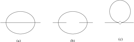
Figure 2: A planar 2-loop diagram (a), with a non-planar divergent subgraph (b). (c) is the 1-loop correction to $\Gamma^{\scriptscriptstyle\{2\}}$ with the 1-loop $\sigma$ correction counterterm. (c) cancels non-planar sub-divergences like (b)

Since the terms in the last two lines of Eq. (25) are $\Lambda_{0}$ independent, UV finiteness of the coupling ${\rm N}_{\scriptscriptstyle m^{2}}[{\widetilde{\Gamma}}_{\Lambda}]$ relies on the UV finiteness of the expression in square brackets. Note the following: the last (divergent) term of this expression — $3\,I^{(2)}_{\Lambda_{R},\,\Lambda_{0}}(0)\,I^{(1)}_{\Lambda_{R},\,\Lambda}$ — originates from the 1-loop contribution to the $\sigma_{0}$ counterterm. This term cancels non-planar sub-divergences of the 2-loop amplitude, like the non-planar sub-divergence of $I^{(3)}$ shown in Figure 2 (b). Had we not included the non-planar coupling $\sigma$ among the marginal ones this counterterm would be absent, and, as we will see temporarily, the amplitude (25) would be UV divergent for $\Lambda\not=\Lambda_{R}$. This shows explicitly that non-planar divergences — at exceptional momenta — also affect the UV behavior of planar amplitudes at higher loops. To show the UV finiteness of ${\rm N}_{\scriptscriptstyle m^{2}}[{\widetilde{\Gamma}}_{\Lambda}]$ let us consider the identity:

$$\!\!\!\!\!\!\!\!\!\!I^{(3)}_{\Lambda,\,\Lambda_{0}}(0)-I^{(3)}_{\Lambda_{R},\,\Lambda_{0}}(0)=-3\!\int\!{dk\over(2\pi)^{4}}\,\Delta_{\Lambda_{R},\,\Lambda}(k)\,I^{(2)}_{\Lambda,\,\Lambda_{0}}(k)\,+$$

$$\qquad-\,I^{(3)}_{\Lambda_{R},\,\Lambda}\!\!-3\!\int\!{dk\over(2\pi)^{4}}\,{dq\over(2\pi)^{4}}\,\Delta_{\Lambda_{R},\,\Lambda}(k)\,\Delta_{\Lambda_{R},\,\Lambda}(q)\,\Delta_{\Lambda,\,\Lambda_{0}}(k+q)$$ (26)

The only UV divergent term in the R.H.S. of the equation above is the integral in the first line, which can be written as

$$-3\!\int\!{dk\over(2\pi)^{4}}\,\Delta_{\Lambda_{R},\,\Lambda}(k)\,I^{(2)}_{\Lambda,\,\Lambda_{0}}(k)=-3\,I^{(1)}_{\Lambda_{R},\,\Lambda}\,I^{(2)}_{\Lambda,\,\Lambda_{0}}(0)+R(\Lambda_{R},\,\Lambda,\,\Lambda_{0})$$ (27)

where $R(\Lambda_{R},\,\Lambda,\,\Lambda_{0})$ is finite as $\Lambda_{0}\to\infty$. The non-planar counterterm $3\,I^{(2)}_{\Lambda_{R},\,\Lambda_{0}}(0)\,I^{(1)}_{\Lambda_{R},\,\Lambda}$ in Eq. (25) is required precisely to cancel the divergence in Eq. (26).

Note that the non-planar counterterm $3\,I^{(2)}_{\Lambda_{R},\,\Lambda_{0}}(0)\,I^{(1)}_{\Lambda_{R},\,\Lambda}$ vanishes at $\Lambda=\Lambda_{R}$. This means that the 2-point renormalized amplitude $\Gamma_{\Lambda}^{\scriptscriptstyle\{2\}}(p)$ would be UV finite at $\Lambda=\Lambda_{R}$ also in a renormalization framework that did not include $\sigma$ among the marginal couplings [1]. The fact that in such a framework the amplitudes at $\Lambda=\Lambda_{R}$ are UV finite while the Wilsonian running couplings (like ${\rm N}_{\scriptscriptstyle m^{2}}[{\widetilde{\Gamma}}_{\Lambda}]$) are not, is the manifestation of the IR/UV difficulty which occurs when one does not take into account non-planar divergences. In the next Section we will generalize this observation by showing that planar renormalized amplitudes of the massive theory evaluated at $\Lambda=\Lambda_{R}$ do not depend on the renormalized coupling $\sigma$. This indeed implies that one can compute planar amplitudes of the massive theory at $\Lambda=\Lambda_{R}$ forgetting about the non-planar marginal coupling $\sigma$. We will also show that this is not true for the massless theory, whose planar amplitudes at $\Lambda=0$ have an “anomalous” dependence on $\sigma$ — this is how the interplay between the IR and the UV manifests itself in our theory, which, nevertheless, is both renormalizable in the Wilsonian sense and completely free of IR/UV divergences.

3 The Parametric Equation

We have seen that renormalization of PIS amplitudes requires including the non-planar coupling $\sigma$ among the relevant couplings. This makes all the amplitudes — both the planar and the non-planar at exceptional momenta — finite. In this Section we will show that, although the renormalized PIS amplitudes depend on four relevant couplings — $m^{2}$, $Z$, $g$ and $\sigma$ — the planar sector of the theory, at $\Lambda=\Lambda_{R}$, is controlled only by three (suitable combinations) of them. Therefore, in a sense, the non-planar coupling $\sigma$ can be thought of as an evanescent coupling of the planar theory: the corresponding counterterm is required to make planar amplitudes UV finite at any scale $\Lambda$, but renormalized planar amplitudes are at $\Lambda=\Lambda_{R}$, essentially, independent of the renormalized value of $\sigma$. To be more precise, we will see that the latter statement is literally correct only for the massive theory. In the massless theory the planar renormalized amplitudes, evaluated at the scale $\Lambda=0$, do depend on $\sigma$: however they satisfy a differential equation of first order in the derivatives with respect to the renormalized couplings. This implies that they are independent of a certain combination of $\sigma$ and $g$. In all cases the planar theory has one less marginal parameter than the full (PIS) theory.

To show this point, we will start by recalling that the RG evolution equation in the large $\theta$ (or, in the case of matrix theories, large $N$) limit is an equation that, unlike the ordinary Wilson-Polchinski RG equation, is of first order in the derivatives of the generating functional with respect to the sources $\Omega_{k}$: it can therefore be written in the form

$$\Lambda\partial_{\Lambda}\,{\widetilde{\Gamma}}_{\Lambda}=R\Bigl{[}\Omega_{k},{\delta{\widetilde{\Gamma}}_{\Lambda}\over\delta\Omega_{k}}\Bigr{]}\equiv R\Bigl{[}\Omega_{k},{\widetilde{\Gamma}}_{\Lambda,\Omega_{k}}\Bigr{]}$$ (28)

where $R$ is the functional of the sources and the first order derivatives of ${\widetilde{\Gamma}}_{\Lambda}$ that appears in the R.H.S. of Eq. (10). Suppose now that the generating functional ${\widetilde{\Gamma}}_{\Lambda}$ satisfies at the scale $\Lambda=\Lambda_{0}$ a differential equation of the form

$$E[{\partial_{\rho_{0}^{\scriptscriptstyle(a)}}{\widetilde{\Gamma}}_{\Lambda_{0}}}]=0$$ (29)

where $E$ is a — not necessarily linear — function of the first order derivatives ${\widetilde{\Gamma}}_{\Lambda}^{\scriptscriptstyle(a)}\equiv{\partial_{\rho_{0}^{\scriptscriptstyle(a)}}}\,{\widetilde{\Gamma}}_{\Lambda}$ of ${\widetilde{\Gamma}}_{\Lambda}$ with respect to the (bare) coupling constants $\rho_{0}^{(a)}$ (with $a$ running over the set $\{m^{2},Z,g,\sigma\}$). It is important that $E$ does not depend explicitly on the sources $\Omega_{k}$. Then

$$\Lambda\partial_{\Lambda}\,E[{\widetilde{\Gamma}}_{\Lambda}^{\scriptscriptstyle(a)}]={\partial E\over\partial{\widetilde{\Gamma}}_{\Lambda}^{\scriptscriptstyle(a)}}\,\Lambda\partial_{\Lambda}\,{\widetilde{\Gamma}}_{\Lambda}^{\scriptscriptstyle(a)}={\partial E\over\partial{\widetilde{\Gamma}}_{\Lambda}^{\scriptscriptstyle(a)}}\,{\delta\,R\over\delta{\widetilde{\Gamma}}_{\Lambda,\Omega_{k}}}\,{\delta{\widetilde{\Gamma}}_{\Lambda}^{\scriptscriptstyle(a)}\over\delta\Omega_{k}}={\delta\,R\over\delta{\widetilde{\Gamma}}_{\Lambda,{\scriptscriptstyle\Omega_{k}}}}\,{\delta E\over\delta\Omega_{k}}$$ (30)

This equation shows that if $E=0$ for $\Lambda=\Lambda_{0}$, $E=0$ identically in $\Lambda$. In particular, we can choose $E$ as follows

$$E=\partial_{\sigma_{0}}{\widetilde{\Gamma}}_{\Lambda}-\Bigl{(}\partial_{m_{0}^{2}}{\widetilde{\Gamma}}_{\Lambda}\Bigr{)}^{2}$$ (31)

Since at the scale $\Lambda_{0}$ $E=0$ by definition, it follows that

$$\partial_{\sigma_{0}}{\widetilde{\Gamma}}_{\Lambda}-\Bigl{(}\partial_{m_{0}^{2}}{\widetilde{\Gamma}}_{\Lambda}\Bigr{)}^{2}=0$$ (32)

for any $\Lambda$. Eq. (32) is the analogue for PIS theory of the celebrated factorization property of large $N$ matrix models

$$\bigl{\langle}\bigl{(}{\rm Tr}\Phi^{k}\bigr{)}^{2}\bigr{\rangle}=\bigl{(}\bigl{\langle}{\rm Tr}\Phi^{k}\bigr{\rangle}\bigr{)}^{2}$$ (33)

From the previous discussion it is apparent that factorization is a direct consequence — in the Wilson-Polchinski framework — of the fact that the RG evolution equation at large $\theta$ or large $N$ is of first order in the derivatives of the generating functional with respect to the sources.

The non-linear parametric equation (32) implies the following linear equation for the generating functional of the planar amplitudes ${\widetilde{\Gamma}}_{\Lambda}^{({\rm pl})}$, the part of ${\widetilde{\Gamma}}_{\Lambda}$ linear in the sources $\Omega_{k}$:

$$\bigl{[}\partial_{\sigma_{0}}-2\,\partial_{\scriptscriptstyle m_{0}^{2}}{\widetilde{\Gamma}}_{\Lambda}^{\scriptscriptstyle\{0\}}\partial_{\scriptscriptstyle m_{0}^{2}}\bigr{]}\,{\widetilde{\Gamma}}_{\Lambda}^{({\rm pl})}=0$$ (34)

where ${\widetilde{\Gamma}}_{\Lambda}^{\scriptscriptstyle\{0\}}$ is the vacuum energy density, the part of ${\widetilde{\Gamma}}_{\Lambda}$ independent of the sources.

We want now to translate the “bare” equation (34) into a renormalized equation. Let us start first with the massive theory. The renormalized generating functional ${\widetilde{\Gamma}}_{\rm ren}\bigl{[}\rho^{\scriptscriptstyle(a)};\Lambda,\Lambda_{R}\bigr{]}$ depends on the renormalized couplings $\rho^{\scriptscriptstyle(a)}$ both through the bare ones and also, as far as the mass is concerned, explicitly via the propagators:

$${\widetilde{\Gamma}}_{\rm ren}\bigl{[}\rho^{\scriptscriptstyle(a)};\Lambda,\Lambda_{R}\bigr{]}\equiv{\widetilde{\Gamma}}_{\Lambda,\,\Lambda_{0}}\bigl{[}\rho_{0}^{\scriptscriptstyle(a)}\bigl{(}\rho^{\scriptscriptstyle(a)};\Lambda_{R},\Lambda_{0}\bigr{)};m^{2}\bigr{]}$$ (35)

Thus

$$\partial_{\scriptscriptstyle\rho_{0}^{\scriptscriptstyle(a)}}={\partial\rho^{\scriptscriptstyle(b)}\over\partial\rho_{0}^{\scriptscriptstyle(a)}}\,\Bigl{[}\partial_{\rho^{\scriptscriptstyle(b)}}-\delta_{b,{\scriptscriptstyle m^{2}}}\,\partial_{\scriptscriptstyle m^{2}}\Bigr{]}$$ (36)

where $\partial_{\scriptscriptstyle m^{2}}$ is the derivative with respect to the explicit $m^{2}$ dependence of the generating functional. Hence

$$\Bigl{[}\bigl{(}\partial_{\sigma_{0}}-2\,\partial_{\scriptscriptstyle m_{0}^{2}}{\widetilde{\Gamma}}_{\Lambda}^{\scriptscriptstyle\{0\}}\partial_{\scriptscriptstyle m_{0}^{2}}\bigr{)}\,\rho^{\scriptscriptstyle(b)}\Bigr{]}\,\Bigl{[}\partial_{\rho^{\scriptscriptstyle(b)}}-\delta_{b,{\scriptscriptstyle m^{2}}}\,\partial_{\scriptscriptstyle m^{2}}\Bigr{]}{\widetilde{\Gamma}}_{\rm ren}^{\rm pl}\bigl{[}\rho^{\scriptscriptstyle(a)};\Lambda,\Lambda_{R}\bigr{]}=0$$ (37)

The previous equation simplifies at the renormalization scale $\Lambda=\Lambda_{R}$. Indeed, acting on Eq. (34) with the normalization operators ${\rm N}_{b}$ (with $b\in\{m^{2},Z,g,\sigma\}$), one obtains

$$\bigl{(}\partial_{\sigma_{0}}-2\,\partial_{\scriptscriptstyle m_{0}^{2}}{\widetilde{\Gamma}}_{\Lambda_{R}}^{\scriptscriptstyle\{0\}}\partial_{\scriptscriptstyle m_{0}^{2}}\bigr{)}\,{\rm N}_{b}[{\widetilde{\Gamma}}_{\Lambda_{R}}^{\rm pl}]=\bigl{(}\partial_{\sigma_{0}}-2\,\partial_{\scriptscriptstyle m_{0}^{2}}{\widetilde{\Gamma}}_{\Lambda_{R}}^{\scriptscriptstyle\{0\}}\partial_{\scriptscriptstyle m_{0}^{2}}\bigr{)}\,\rho^{\scriptscriptstyle(b)}=0$$ (38)

for all planar couplings $\rho^{\scriptscriptstyle(b)}$, i.e. for $b\not=\sigma$. Thus Eq. (37) reduces for $\Lambda=\Lambda_{R}$ to

$$\partial_{\sigma}\,{\widetilde{\Gamma}}_{\rm ren}^{\rm pl}\bigl{[}\rho^{\scriptscriptstyle(a)};\Lambda_{R},\Lambda_{R}\bigr{]}=0$$ (39)

since $\bigl{(}\partial_{\sigma_{0}}-2\,\partial_{\scriptscriptstyle m_{0}^{2}}{\widetilde{\Gamma}}_{\Lambda_{R}}^{\scriptscriptstyle\{0\}}\partial_{\scriptscriptstyle m_{0}^{2}}\bigr{)}\,\sigma\not=0$. The parametric equation (39) shows that planar amplitudes of the massive theory evaluated at the renormalization scale $\Lambda_{R}$ are independent of the non-planar coupling $\sigma$. For example, from Eq. (24), one sees that $\partial_{\sigma}\Gamma^{\scriptscriptstyle\{2\}}_{\Lambda,\Lambda_{R}}$ vanishes at $\Lambda=\Lambda_{R}$. The parametric equation (39) also means that if we consider ${\widetilde{\Gamma}}_{\rm ren}^{\rm pl}$ at $\Lambda=\Lambda_{R}$ as function of the renormalized $m^{2},Z,g$ and of the bare $\sigma_{0}$, it does not depend on $\sigma_{0}$. In other words in the massive theory one can forget about the $\sigma$ coupling if one only wants to compute planar amplitudes at $\Lambda=\Lambda_{R}$.

The massless case is more subtle and thus more interesting. Because of the massless renormalization condition (18) there is one less renormalized coupling than there are bare couplings. The renormalization conditions for $Z$, $g$ and $\sigma$ in Eq. (17) express the renormalized couplings $\rho^{\scriptscriptstyle(\alpha)}$, where $\alpha\in\{Z,g,\sigma\}$, as functions of the bare couplings $\rho^{\scriptscriptstyle(\beta)}_{0}$ and $m_{0}^{2}$:

$$\rho^{\scriptscriptstyle(\alpha)}=\rho^{\scriptscriptstyle(\alpha)}(\rho^{\scriptscriptstyle(\beta)}_{0},m_{0}^{2};\Lambda_{R},\Lambda_{0})$$ (40)

where $\Lambda_{R}>0$ to regulate the infrared divergences. The massless renormalization condition (18) determines $m_{0}^{2}=m_{0}^{2}(\rho^{\scriptscriptstyle(\beta)}_{0};\Lambda_{0})$ as function of the bare $\rho^{\scriptscriptstyle(\beta)}_{0}$: by substituting this latter expression into Eq. (40) one obtains the renormalized $\rho^{\scriptscriptstyle(\alpha)}$ as functions of the bare $\rho_{0}^{\scriptscriptstyle(\beta)}$:

$$\rho^{\scriptscriptstyle(\alpha)}=\rho^{\scriptscriptstyle(\alpha)}(\rho^{\scriptscriptstyle(\beta)}_{0},m_{0}^{2}(\rho^{\scriptscriptstyle(\beta)}_{0};\Lambda_{0});\Lambda_{R},\Lambda_{0})$$ (41)

From now on when writing $\rho^{\scriptscriptstyle(\alpha)}$ we refer to the functions of $\rho^{\scriptscriptstyle(\beta)}_{0}$ defined in the equation above: denoting by $\rho_{0}^{(\beta)}(\rho^{(\alpha)};\Lambda_{R},\Lambda_{0})$ their inverses, the renormalized functional is defined by

$${\widetilde{\Gamma}}_{\rm ren}\bigl{[}\rho^{\scriptscriptstyle(\alpha)};\Lambda,\Lambda_{R}\bigr{]}\equiv{\widetilde{\Gamma}}_{\Lambda,\,\Lambda_{0}}\bigl{[}\rho_{0}^{\scriptscriptstyle(\beta)}\bigl{(}\rho^{\scriptscriptstyle(\alpha)};\Lambda_{R},\Lambda_{0}\bigr{)},m_{0}^{2}(\rho^{\scriptscriptstyle(\beta)}_{0}(\rho^{\scriptscriptstyle(\alpha)};\Lambda_{R},\Lambda_{0});\Lambda_{0})\bigr{]}$$ (42)

Therefore

$$\partial_{\rho^{\scriptscriptstyle(\alpha)}}={\partial\rho_{0}^{\scriptscriptstyle(\beta)}\over\partial\rho^{\scriptscriptstyle(\alpha)}}\,{\partial\over\partial\rho_{0}^{\scriptscriptstyle(\beta)}}+{\partial m_{0}^{2}\over\partial\rho^{\scriptscriptstyle(\alpha)}}\,{\partial\over\partial m_{0}^{2}}$$ (43)

and thus

$${\partial\rho^{\scriptscriptstyle(\alpha)}\over\partial\sigma_{0}}{\partial{\widetilde{\Gamma}}_{\rm ren}^{\rm pl}\over\partial\rho^{\scriptscriptstyle(\alpha)}}={\partial{\widetilde{\Gamma}}^{\rm pl}_{\Lambda}\over\partial\sigma_{0}}+{\partial\rho^{\scriptscriptstyle(\alpha)}\over\partial\sigma_{0}}\,{\partial m_{0}^{2}\over\partial\rho^{\scriptscriptstyle(\alpha)}}\,{\partial{\widetilde{\Gamma}}^{\rm pl}_{\Lambda}\over\partial m_{0}^{2}}={\partial{\widetilde{\Gamma}}^{\rm pl}_{\Lambda}\over\partial\sigma_{0}}+{\partial m_{0}^{2}\over\partial\sigma_{0}}\,{\partial{\widetilde{\Gamma}}^{\rm pl}_{\Lambda}\over\partial m_{0}^{2}}$$ (44)

Using the parametric bare equation (34) we obtain

$${\partial\rho^{\scriptscriptstyle(\alpha)}\over\partial\sigma_{0}}{\partial{\widetilde{\Gamma}}_{\rm ren}^{\rm pl}\over\partial\rho^{\scriptscriptstyle(\alpha)}}[\Lambda,\Lambda_{R}]=\Bigl{[}2\,\partial_{\scriptscriptstyle m_{0}^{2}}{\widetilde{\Gamma}}_{\Lambda}^{\scriptscriptstyle\{0\}}+{\partial m_{0}^{2}\over\partial\sigma_{0}}\Bigr{]}\,{\partial{\widetilde{\Gamma}}_{\Lambda}^{\rm pl}\over\partial m_{0}^{2}}$$ (45)

To evaluate ${\partial m_{0}^{2}\over\partial\sigma_{0}}$ we make use of the massless renormalization condition (18), which gives

$${\partial m_{0}^{2}\over\partial\sigma_{0}}=-\Biggl{[}{\partial\,{\rm N}_{\scriptscriptstyle m^{2}}[{\widetilde{\Gamma}}_{\scriptscriptstyle\Lambda=0}]\over\partial m_{0}^{2}}\Biggr{]}^{-1}\,{\partial\,{\rm N}_{\scriptscriptstyle m^{2}}[{\widetilde{\Gamma}}_{\scriptscriptstyle\Lambda=0}]\over\partial\sigma_{0}}$$ (46)

Substituting into Eq. (45), one gets

$${\partial\rho^{\scriptscriptstyle(\alpha)}\over\partial\sigma_{0}}{\partial{\widetilde{\Gamma}}_{\rm ren}^{\rm pl}\over\partial\rho^{\scriptscriptstyle(\alpha)}}[\Lambda,\Lambda_{R}]=-{\partial{\widetilde{\Gamma}}_{\Lambda}^{\rm pl}\over\partial m_{0}^{2}}\,\Biggl{[}{\partial\,{\rm N}_{\scriptscriptstyle m^{2}}[{\widetilde{\Gamma}}_{\scriptscriptstyle\Lambda=0}]\over\partial m_{0}^{2}}\Biggr{]}^{\scriptstyle-1}\!\Bigl{[}\partial_{\sigma_{0}}-2\,\partial_{\scriptscriptstyle m_{0}^{2}}{\widetilde{\Gamma}}_{\Lambda}^{\scriptscriptstyle\{0\}}\,\partial_{\scriptscriptstyle m_{0}^{2}}\Bigr{]}\,{\rm N}_{\scriptscriptstyle m^{2}}[{\widetilde{\Gamma}}_{\scriptscriptstyle\Lambda=0}]$$ (47)

This equation simplifies considerably when evaluated at $\Lambda=0$, since then the R.H.S. becomes proportional to the bare parametric equation and hence vanishes:

$$R^{\scriptscriptstyle(\alpha)}\,{\partial{\widetilde{\Gamma}}_{\rm ren}^{\rm pl}\over\partial\rho^{\scriptscriptstyle(\alpha)}}[\Lambda,\Lambda_{R}]\big{|}_{\Lambda=0}=0$$ (48)

where

$$R^{\scriptscriptstyle(\alpha)}\equiv{\partial\rho^{\scriptscriptstyle(\alpha)}\over\partial\sigma_{0}}$$ (49)

The derivative of ${\widetilde{\Gamma}}_{\rm ren}^{\rm pl}$ with respect to $Z$ which appear in Eq. (48) can be replaced by $g$ and $\sigma$ derivatives by using the so-called counting identity. This identity takes the following simple form when evaluated at $\Lambda=0$

$$Z\partial_{Z}\,{\widetilde{\Gamma}}^{\scriptscriptstyle\{k\}}_{\rm ren}[0,\Lambda_{R}]=\Bigl{[}{k\over 2}-2(g\partial_{g}+\sigma\partial_{\sigma})\Bigr{]}\,{\widetilde{\Gamma}}^{\scriptscriptstyle\{k\}}_{\rm ren}[0,\Lambda_{R}]$$ (50)

where ${\widetilde{\Gamma}}^{\scriptscriptstyle\{k\}}_{\rm ren}[\Lambda,\Lambda_{R}]$ is the planar amplitude with $k$ external legs. Therefore, choosing $Z=1$, one can rewrite Eq. (48) as follows

$$\bigl{[}\partial_{\sigma}+\chi\,\partial_{g}+\tau\bigr{]}\,{\widetilde{\Gamma}}_{\rm ren}^{\scriptscriptstyle\{k\}}[0,\Lambda_{R}]=0$$ (51)

where we introduced the generalized beta-functions

$$\chi(g,\sigma)={R^{\scriptscriptstyle(g)}-2\,g\,R^{\scriptscriptstyle(Z)}\over R^{\scriptscriptstyle(\sigma)}-2\,\sigma\,R^{\scriptscriptstyle(Z)}}\qquad\quad\tau(g,\sigma)={1\over 2}\,{k\,R^{\scriptscriptstyle(Z)}\over R^{\scriptscriptstyle(\sigma)}-2\,\sigma\,R^{\scriptscriptstyle(Z)}}$$ (52)

We will see in a moment that $\chi$ and $\tau$ get their first non-vanishing contributions at 2 and 3 loops respectively. The generalized beta-functions (52) capture therefore the “anomalous” dependence of the planar amplitudes on the non-planar renormalized coupling $\sigma$ in the massless theory: this effect, as it will be apparent from the computation that follows, is due to an interplay between the UV and IR divergences of the theory.

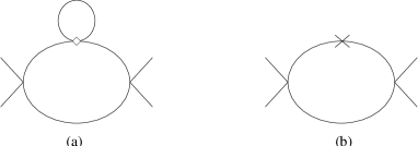
Figure 3: $\sigma$-dependent 2-loops corrections to $\Gamma^{\scriptscriptstyle\{4\}}$. The diamond is the $\sigma$ vertex and the cross the mass counterterm insertion

From Eqs. (23) it follows that

$$R^{\scriptscriptstyle(Z)}=O(\hbar^{3})\qquad\qquad R^{\scriptscriptstyle(\sigma)}=1+O(\hbar)$$ (53)

The first non-vanishing contributions to $R^{\scriptscriptstyle(g)}$ come from the 2 loop diagrams in Figure 3. Therefore $\tau(g,\sigma)=O(\hbar^{3})$ and

$$\chi(g,\sigma)=R^{\scriptscriptstyle(g)}_{\scriptscriptstyle 2\,loops}+O(\hbar^{3})$$ (54)

Up to order $O(\hbar^{3})$ the $\sigma_{0}$ dependence of $g$ is given by the expression

$$g=g_{0}+2\,g_{0}^{2}\,I^{(2)}_{\Lambda_{R},\,\Lambda_{0}}(0)+4\,\sigma_{0}\,g_{0}^{2}\,I^{(1)}_{\Lambda_{R},\,\Lambda_{0}}\,I^{(4)}_{\Lambda_{R},\,\Lambda_{0}}(0)+4\,m^{2}_{0}\,g_{0}^{2}\,I^{(4)}_{\Lambda_{R},\,\Lambda_{0}}(0)+O(g_{0}^{3})$$ (55)

where

$$I^{(4)}_{\Lambda_{R},\,\Lambda_{0}}(p)\equiv\int\!{dk\over(2\pi)^{4}}\,(\Delta_{\Lambda,\,\Lambda_{0}}(k))^{2}\,\Delta_{\Lambda,\,\Lambda_{0}}(k-p)$$ (56)

$m^{2}_{0}$ as a function of $\sigma_{0}$ and $g_{0}$ at 1 loops is determined by the first of Eqs. (23) evaluated for $\Lambda_{R}=0$:

$$m^{2}_{0}=-(\sigma_{0}+2\,g_{0})I^{(1)}_{0,\,\Lambda_{0}}+O(\hbar^{2})$$ (57)

Plugging this expression into Eq. (55) one obtains for the beta function $\chi(g,\sigma)$ at two loops the following result

$$R^{\scriptscriptstyle(g)}_{\scriptscriptstyle 2\,loops}=-4\,g^{2}\,I^{(1)}_{0,\,\Lambda_{R}}\,I^{(4)}_{\Lambda_{R},\,\Lambda_{0}}(0)=-{4\,g^{2}\over(16\pi^{2})^{2}}\,\Lambda_{R}^{2}\,\Bigl{(}{1\over\Lambda_{R}^{2}}-{1\over\Lambda_{0}^{2}}\Bigr{)}\,{\mathop{\longrightarrow}^{\scriptscriptstyle\Lambda_{0}\to\infty}}\,-{g^{2}\over 64\,\pi^{4}}$$ (58)

Let us verify the massless parametric equation (51) for the planar 4-point function at 2 loops, the lowest order for which the equation is non-trivial. Let us choose, just for simplicity, the external momenta $(p_{1},p_{2},p_{3},p_{4})$ equal to $(p,0,-p,0)$. The bare 4-point function becomes:

$$\!\!\!\!\!\!\!\!\!\!\!\!\!\!\!\!\!\!\Gamma^{\scriptscriptstyle\{4\}}_{\Lambda,\,\Lambda_{0}}(p)=g_{0}+2\,g_{0}^{2}\,I^{(2)}_{\Lambda,\,\Lambda_{0}}(p)+4\,g_{0}^{2}\,\Bigl{(}\sigma_{0}\,I^{(1)}_{\Lambda,\,\Lambda_{0}}+m^{2}_{0}\Bigr{)}\,I^{(4)}_{\Lambda,\,\Lambda_{0}}(p)+O(g_{0}^{3})=$$

$$\quad\!=g_{0}+2\,g_{0}^{2}\,I^{(2)}_{\Lambda,\,\Lambda_{0}}(p)-4\,\sigma_{0}\,g_{0}^{2}\,I^{(1)}_{0,\,\Lambda}\,I^{(4)}_{\Lambda,\,\Lambda_{0}}(p)+O(g_{0}^{3})$$ (59)

where in the second line of the equation above we used the masslessness constraint (57). Substituting now bare with renormalized couplings (using Eq. (55)), we find that the renormalized 4-point function is given by the $\Lambda_{0}\to\infty$ limit of the following expression:

$$\!\!\!\!\!\!\!\!\!\!\Gamma^{\scriptscriptstyle\{4\}}_{\Lambda,\,\Lambda_{0};\,\Lambda_{R}}(p)=g-2\,g^{2}\,\Bigl{(}I^{(2)}_{\Lambda,\,\Lambda_{0}}(p)-I^{(2)}_{\Lambda_{R},\,\Lambda_{0}}(0)\Bigr{)}+$$

$$\qquad\qquad-4\,\sigma\,g^{2}\,\Bigl{(}I^{(1)}_{0,\,\Lambda}\,I^{(4)}_{\Lambda,\,\Lambda_{0}}(p)-I^{(1)}_{0,\,\Lambda_{R}}\,I^{(4)}_{\Lambda_{R},\,\Lambda_{0}}(0)\Bigr{)}+O(g^{3})$$ (60)

We thus see that the L.H.S. of the parametric equation (51), applied to the 4-point planar function, equals

$$\bigl{[}\partial_{\sigma}+\chi\,\partial_{g}+\tau\bigr{]}\,\Gamma^{\scriptscriptstyle\{4\}}_{\rm ren}(p)[0,\Lambda_{R}]=-4\,g^{2}\,\lim_{\Lambda\to 0\atop}\,I^{(1)}_{0,\,\Lambda}\,I^{(4)}_{\Lambda,\,\infty}(p)$$ (61)

Since

$$-4\,g^{2}\,I^{(1)}_{0,\,\Lambda}\,I^{(4)}_{\Lambda,\,\infty}(p)={g^{2}\over(16\,\pi^{2})^{2}}\,{\Lambda^{2}\over p^{2}}\,\Bigl{[}\log\,\Bigl{(}{\Lambda^{2}\over p^{2}}\Bigr{)}-1+O\Bigl{(}{\Lambda^{2}\over p^{2}}\Bigr{)}\Bigr{]}$$ (62)

the R.H.S. of the Eq. (61) vanishes. Note that the $\Lambda\to 0$ limit of Eq. (61) must be defined by taking $\Lambda/p\to 0$.

4 Conclusions

The main message of this article is that, even at $\theta=\infty$, renormalized non-commutative field theories do not reduce simply to their planar sector. The genus zero RG equation couples planar amplitudes to partially integrated non-planar amplitudes. Since the dependence of PIS amplitudes on $\theta$ factors out, these amplitudes are essentially the same as in matrix field theory. While the non-planar coupling $\sigma$ can be introduced in a local way in $N\times N$ matrix field theory at finite $N$ — via the multi-trace operator $\int dx({\rm Tr}\phi^{2}(x))^{2}$ — this is not possible in the non-commutative theory of the Moyal type, since in this kind of theories every trace must be accompanied by integration over non-commutative space. The Wilson-Polchinski genus zero equation allows for a perfectly rigorous treatment of the non-local, non-planar “bare” coupling in Eq. (19) and elucidates the mechanism by which this non-local counterterm cancels local (planar) divergences of planar amplitudes.

The genus zero RG equation also clarifies the standing and the limitations of the purely planar renormalization [1] of non-commutative field theories. A distinguishing feature of the genus zero RG equation is of being of first order in source derivatives: we showed that this entails factorization, a well-known property of large $N$ matrix models. One might expect, because of factorization, to be able to disregard the non-planar counterterms altogether when computing planar amplitudes in the limit $\theta\to\infty$ (or, in the matrix field theory case, in the limit $N\to\infty$). We showed that this is not quite so. In the massive theory factorization implies that one can indeed remove UV divergences of planar amplitudes using only planar counterterms, if one keeps the floating Polchinski cut-off $\Lambda$ equal to the renormalization scale $\Lambda_{R}$ that defines the renormalized couplings. In the usual, commutative, situation UV finiteness of $\Gamma_{\Lambda,\Lambda_{R}}$ at $\Lambda=\Lambda_{R}$ would imply its finiteness for any $\Lambda$, since the Wilson-Polchinski RG equation is essentially independent of the UV cut-off. In the non-commutative case instead this is not the case: if one insists on introducing only planar counterterms as soon as $\Lambda$ differs from $\Lambda_{R}$, the UV scale $\Lambda_{0}$ reappears in the effective planar action. The reason, of course, is that the RG equation does not close on planar amplitudes and the $\Lambda$ derivative of a planar amplitudes involves non-planar diagrams evaluated at exceptional momenta (see Figure 2), which — in planar renormalization — are divergent. The situation for the massless theory is even more dramatic: planar counterterms are not enough to eliminate UV divergences even if one sends the floating cut-off to the renormalization scale, i.e. even in the limit $\Lambda\to 0$.

The restriction to partially integrated amplitudes also elucidates the nature of non-planar contributions to non-commutative current algebra anomalies [8]. The non-planar part of the topological charge which captures the axial non-commutative anomaly appears in the effective action as a partially integrated non-local term of the type in Eq. (19). To give an example in 2 dimensions, let $A_{\mu}$ be the axial vector field to which the axial current is coupled, $V_{\mu}$ the background vector field which couples to the vector current and $F_{\mu\nu}$ the field strength relative to $V_{\mu}$. Then the non-planar anomaly computed in in [8] is reproduced by a term in the effective action that, written in (non-commutative) configuration space, writes as

$$\lim_{\Lambda\to 0}\Lambda^{2}\int\!\!d^{2}x\,{{\rm e}^{-\Lambda^{2}\,x^{2}}\over 2\pi^{2}}{1\over{\partial}^{\,2}}\,\partial_{\mu}A_{\mu}(x)\int\!d^{2}y\,\epsilon^{\mu\nu}F_{\mu\nu}(y)$$ (63)

very much analogous to the partially integrated non-local term in Eq. (19).

One can think of several possible extensions of our work. The most challenging is the construction of a renormalized theory of partially integrated amplitudes at higher genus. The analysis of partially integrated amplitudes of genus $g$, that we present in Appendix B, shows that these amplitudes go as $1/{\theta}^{dg}$ for large $\theta$ — unlike amplitudes at generic external momenta which do not have a $\theta=\infty$ limit uniform in the external momenta. This strongly suggests that renormalized partially integrated amplitudes at higher genus admit a meaningful $1/{\theta}$ expansion. Attacking the renormalization problem of higher genus amplitudes necessitates first of all working out the corresponding expansion of the Wilson-Polchinski RG equation. The RG evolution of higher genus partially integrated amplitudes involves lower genus amplitudes with non-vanishing total momenta flowing into two of their holes: for this reason it seems that the understanding of the higher genus non-commutative theory might require significantly extending the ideas presented in this paper. It is a problem that we leave for the future. Another issue which emerges from the present work is the interpretation of the restriction to partially integrated amplitudes from string theory point of view. One might also consider extending our analysis to gauge non-commutative theories.

Appendix A Moyal Phases for Spherical Amplitudes

In this appendix we derive a formula for the $\theta$ dependence of generic spherical Feynman diagram integrands.

Recall that planar diagrams depend on $\theta$ via the Moyal factor

$${\rm e}^{-i\,\Phi_{n}(p_{1},\ldots,p_{n})}\equiv{\rm e}^{-i\sum_{i<j}p_{i}\wedge p_{j}}$$ (64)

where $p_{1}\wedge p_{2}\equiv{1\over 2}\theta_{\mu\nu}\,p_{1}^{\mu}\,p_{2}^{\nu}$, and $p_{1},\ldots,p_{n}$ are the momenta associated to the $n$ external lines of the graph. Let us briefly review the derivation of Eq. (64) which exploits the following property of planar double-line graphs: the momentum through any propagator (or external line) in the graph can be written as the difference $l_{i}-l_{j}$ where $l_{i}$ and $l_{j}$ are pseudo-momenta associated with the (oriented) single lines that are the adjacent edges of the double-line propagator. For any vertex with $k$ legs, let the momenta entering the vertex be $q_{1},q_{2},\ldots,q_{k},$ in cyclic order: with respect to the commutative theory, the Feynman rules of the Moyal non-commutative theory include the additional phase factor

$${\rm e}^{-i\,\Phi_{k}(q_{1},\ldots,q_{k})}={\rm e}^{-i\sum_{i<j}q_{i}\wedge q_{j}}$$ (65)

Writing the momenta $q_{j}$ in terms of pseudo-momenta, $q_{j}=l_{i_{j}}-l_{i_{j+1}}$, one obtains

$$\sum_{i<j}q_{i}\wedge q_{j}=l_{i_{1}}\wedge l_{i_{2}}+l_{i_{2}}\wedge l_{i_{3}}+\cdots+l_{i_{n}}\wedge l_{i_{1}}$$ (66)

Thus the phase factor at any interaction point may be expressed as the product of $k$ terms, one for each incoming propagator

$${\rm e}^{-i\,\Phi_{k}(q_{1},\ldots,q_{k})}=\prod_{j=1}^{k}e^{-i\,(l_{i_{j}}\wedge\,l_{i_{j+1}})}$$ (67)

Any internal propagator gives two contributions to the total phase factor (64) — one for each of its two end vertices — which cancel each other. Therefore only the external momenta contribute to the total phase factor, and one obtains Eq. (64).

The representation of propagator momenta in terms of pseudo-momenta is valid not only for the planar diagrams but, more generally, also for PIS amplitudes. Therefore the very same argument which leads to Eq. (64) generalizes to PIS amplitudes with $h$ holes: every hole with $k$ external lines gives a phase factor ${\rm e}^{-i\Phi_{k}}$, and hence the total Moyal phase of the amplitude is the product of $h$ factors like in (64), one for each hole.

Let us now turn to generic non-planar spherical diagrams with $h$ holes. Let $a=1,\ldots,h$ be a label defining an arbitrary order of the holes. Let $p^{(a)}_{i_{a}}$, with $i_{a}=1,\ldots,n_{a}$, be the $i_{a}$-th momentum entering the $a$-th hole of the spherical amplitude. The $n_{a}$ momenta entering the hole have a natural cyclic order determined by the orientation of the associated Riemann surface: thus, defining the indices $i_{a}$ requires choosing a particular (first) momentum for each hole. A spherical diagram with $L$ loops defines a triangulation of the sphere with $F=L+1$ faces. We called holes the faces to which external lines are attached, and thus, obviously, $h\leq F=L+1$. We denote by $q_{A}$, with $A=1,\ldots,L$ the independent loop momenta, arbitrarily chosen. The Moyal phase $\Phi\,(q_{A},p^{(a)}_{i_{a}})$ of the diagram has the general structure

$$\Phi\,(q_{A},p^{(a)}_{i_{a}})=\!\sum_{A,B}C_{AB}\,q_{A}\wedge\,q_{B}+\!\sum_{a,\,A,\,i_{a}}\!\!D^{(a)}_{A\,i_{a}}q_{A}\wedge p^{(a)}_{i_{a}}+\!\sum_{a,\,b,\,i_{a},\,i_{b}}\!\!\!\!\!E^{(ab)}_{i_{a}i_{b}}\,p^{(a)}_{i_{a}}\wedge\,p^{(b)}_{i_{b}}$$ (68)

where $C_{AB}$, $D^{(a)}_{A\,i_{a}}$ and $E^{(ab)}_{i_{a}i_{b}}$ are constant coefficients.

When all the external momenta $p^{(a)}_{i_{a}}$ vanish, the amplitude becomes planar with no external lines and, thus, the Moyal phase vanish: it follows that $C_{AB}=0$. Also, if all the loop momenta $q_{A}$ vanish, the resulting Moyal phase is that of the tree — and hence planar — diagram obtained from the original diagram by cutting all the internal propagators associated with the momenta $q_{A}$. This tree diagram has the external lines of the original diagram, with an ordering which depends on the choice of the cut propagators, i.e. on the choice of the $L$ independent loop momenta $q_{A}$. Our choice of ordering of the holes and of the “first” momenta of each hole (implicit in the definition of the indices $a$ and $i_{a}$) induces, of course, an ordering on the external momenta: we can always take this ordering to coincide with the ordering of the external momenta of the tree diagram above. In other words, the (arbitrary) definition of the loop momenta $q_{A}$ should be consistent with the (arbitrary) definition of the indices $a$ and $i_{a}$. With this understanding, $\Phi(0,p^{(a)}_{i_{a}})$ writes as

$$\Phi(0,p^{(a)}_{i_{a}})=\!\sum_{a,\,b,\,i_{a},\,i_{b}}\!\!\!\!\!E^{(ab)}_{i_{a}i_{b}}\,p^{(a)}_{i_{a}}\wedge\,p^{(b)}_{i_{b}}=\sum_{a}\!\sum_{i_{a}<j_{a}}\!p^{(a)}_{i_{a}}\wedge\,p^{(a)}_{j_{a}}+\sum_{a<b}\Sigma^{(a)}\wedge\,\Sigma^{(b)}$$ (69)

where $\Sigma^{(a)}\equiv\sum_{i_{a}}\!p^{(a)}_{i_{a}}$ is the momentum entering the $a$-th hole. Last, let us take all the $\Sigma^{(a)}=0$: the amplitude becomes PIS and thus its Moyal phase reduces to $\sum_{a}\!\sum_{i_{a}<j_{a}}\!p^{(a)}_{i_{a}}\wedge\,p^{(a)}_{j_{a}}$. Hence the term $\sum_{a,\,A,\,i_{a}}\!\!D^{(a)}_{A\,i_{a}}q_{A}\wedge p^{(a)}_{i_{a}}$ in (68) must vanish when $\Sigma^{(a)}=0$ and therefore it can be expressed as linear combination of the $\Sigma^{(a)}$

$$\sum_{a,\,A,\,i_{a}}\!\!D^{(a)}_{A\,i_{a}}q_{A}\wedge p^{(a)}_{i_{a}}=\!\sum_{a}k^{(a)}\wedge\,\Sigma^{(a)}$$ (70)

where $k^{(a)}$ are $h$ linear combinations of the $L$ loop momenta $q_{A}$. In conclusion the Moyal phase of the diagram is

$$\Phi\,(k^{(a)},p^{(a)}_{i_{a}})=\sum_{a}\!\sum_{i_{a}<j_{a}}\!p^{(a)}_{i_{a}}\wedge\,p^{(a)}_{j_{a}}+\sum_{a<b}\Sigma^{(a)}\wedge\,\Sigma^{(b)}+\!\sum_{a}k^{(a)}\wedge\,\Sigma^{(a)}$$ (71)

The last term in the R.H.S. of Eq. (71) gives an IR sensitive UV cut-off for the integrand of the corresponding Feynman amplitude — the origin of the famous IR-UV mixing effect. Because of this term, the Feynman integral is not — for $\Sigma^{(a)}\not=0$ — an analytic function of the non-commutative parameter $\theta$ at $\theta=\infty$. As we mentioned above, PIS amplitudes (for which $\Sigma^{(a)}=0$) are precisely those that admit a good $\theta\to\infty$ limit: for them, the R.H.S. of Eq. (71) reduces to the first term, which, thanks to momentum conservation, is now independent of the ordering choices underlying the definition of the indices $a$ and $i_{a}$.

An explicit definition for the $h$ loop momenta $k^{(a)}$ in Eq. (71) can be given as follows. Take the original non-planar diagram and put to zero all the external momenta $p^{(a)}_{i_{a}}$. The resulting diagram is planar and its internal momenta admit the EK representation in terms of pseudo-momenta $l_{A}$, with $A=1,\ldots L+1$, one for each face of the diagram. To take into account the external momenta consider also an auxiliary oriented path running through the double-line propagators with the following properties: (i) the path connects all the points to which the external legs are attached; (ii) it turns clockwise around each hole starting from the arbitrary chosen “first” leg to the “last” and going from the arbitrary chosen “first” hole to the “last” (thus defining an ordering of the external legs); (iii) the path together with the external legs attached to it forms a tree diagram whose propagators carry the momenta which enter through the external legs. An example of such auxiliary momentum path is depicted in Figure 4.

Figure 4: A spherical non-planar diagram with two holes and its auxiliary momentum path

The EK prescription for the momentum $k^{(a)}$ flowing through a given propagator is now corrected by adding to the pseudo-momenta contribution the momenta carried by the path, if this happens to go through the propagator. With this definition of the internal $k^{(a)}$ the Moyal phase (71) of a spherical non-planar diagram writes as

$$\Phi\,(l_{a},p^{(a)}_{i_{a}})=\sum_{a}\!\sum_{i_{a}<j_{a}}\!p^{(a)}_{i_{a}}\wedge\,p^{(a)}_{j_{a}}+\sum_{a<b}\Sigma^{(a)}\wedge\,\Sigma^{(b)}+\!2\,\sum_{a}l_{a}\wedge\,\Sigma^{(a)}$$ (72)

where $l_{a}$ with $a=1,\ldots,h\leq L+1$ are the pseudo-momenta associated with the holes. Since $\sum_{a}\Sigma^{(a)}=0$, $\Phi\,(l_{a},p^{(a)}_{i_{a}})$ is invariant under $l_{a}\to l_{a}+c$, and thus depends only on the differences of the pseudo-momenta $l_{a}$.

Appendix B Moyal phases for higher genus amplitudes

In this appendix we will analyze the $\theta$ dependence of non-spherical amplitudes.

Let us begin with the following remark: the Moyal phase associated with a double-line diagram is invariant under topological deformations of the type depicted in Figure 5. These are deformations which vary the lengths of the double-line propagators and correspond to changing the triangulation of the underlying Riemann surface by keeping fixed its genus $g$ and its number $F$ of faces. Note that the number of loops $L$ of the Feynman diagram, which is given by

$$L=F-1+2\,g\,,$$ (73)

is left unchanged by these deformations.

Figure 5: Topological deformations preserving the Moyal phases

Consider now a diagram of genus $g$ and $F$ faces and join with a double-line propagator two external legs attached to two different holes: one obtains in this way a diagram of genus $g+1$ and $F-1$ faces. This follows from the Euler relation $2-2g=F-E+V$, where $V$, $E$ and $F$ are the numbers of vertices, propagators and faces of the diagram: the new diagram has the same number of vertices, one more propagator and one face less than the original diagram and, thus, one more handle. Therefore we can build diagrams of any genus $g$ and any number of faces $F$ starting from spherical (non-planar) diagrams with $g+F$ faces by means of the following construction: Consider one such spherical diagram and join $g$ pairs of external legs with $g$ propagators — choosing the legs of each pair to belong to different holes. In other words there should be at most a single double-line propagator connecting any pair of holes. An example of this construction for a genus 2 surface built out of a spherical diagram with 3 holes and 4 external legs is given in Figure 6.

An important result in the theory of Riemann surfaces states that double-line diagrams with fixed $g$ and $F$ provide a cell decomposition of the moduli space of oriented Riemann surfaces of genus $g$ and $F$ boundaries: the moduli of Riemann surfaces are parametrized by non-negative real numbers associated with the lengths of the double-line propagators. Since the moduli space of fixed genus and fixed number of boundaries is a connected variety, it follows that one can transform, by means of the deformations in Figure 5, any graph of genus $g$ and $F$ faces into a topologically equivalent one built out of spherical non-planar diagrams in the way explained in the previous paragraph.

Given two topologically equivalent diagrams, their loop momenta are in a one-to-one correspondence and thus can be identified: under this identification their Moyal phases coincide. We can therefore limit ourselves to evaluate the Moyal phase of the higher genus diagrams built out of spherical non-planar graphs. The Moyal phases of such graphs are given by the formula in Eq. (72) for the associated non-planar spherical graphs where some of the external momenta $p^{(a)}_{i_{a}}$ — those flowing into the legs which are joined by the $g$ propagators — become loop momenta, $q_{i}$ (with $i=1,\ldots,g$) of the higher genus diagrams. Thus we can write the sum $\Sigma^{(a)}$ of the momenta entering the $a$-th hole, which appears in Eq. (72), as follows:

$$\Sigma^{(a)}=\sum_{i=1}^{g}q_{i}\,e_{i}^{a}+P^{(a)}$$ (74)

In the formula above $P^{(a)}$ is momentum carried by the external legs of the higher genus diagram attached to the $a$-th hole of the corresponding spherical diagram; $e_{i}^{a}$ is a numerical matrix whose $(i,a)$-th element is +1 (-1) if the momentum $q_{i}$ enters (leaves) the $a$-th hole and 0 otherwise. $e_{i}^{a}$ is the incidence matrix of the graph whose points are the holes of the non-planar spherical diagram and whose lines are the $g$ propagators which connect the holes. This is a tree graph because any pair of holes is

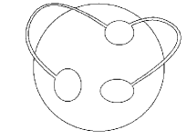
Figure 6: A genus 2 surface from a sphere with 3 holes and 4 external legs

connected at most by a single propagator.

The Moyal phase of the higher genus diagram is therefore a quadratic form in the loop momenta $l_{a}$ and $q_{i}$ which looks as follows:

$$\Phi_{higher-genus}=\sum_{i,j}C_{ij}\,q_{i}\wedge\,q_{j}+2\sum_{i,\,a}e_{i}^{a}\,l_{a}\wedge q_{i}+A$$ (75)

where $C_{ij}$ is a numerical matrix and $A$ is at most linear in the loop momenta. Since $\sum_{i,\,a}e_{i}^{a}\,q_{i}=0$, the Moyal phase $\Phi_{higher-genus}$ depends only on the differences of the $l_{a}$’s. In conclusion, the part of $\Phi_{higher-genus}$ quadratic in the loop momenta $Q_{A}\equiv(l_{a},q_{i})$ can be written as $\sum_{A,B}D_{AB}\,Q_{A}\wedge Q_{B}$ where $D_{AB}$ is an anti-symmetric matrix of the following form

$$(D)_{AB}=\left(\matrix{0&e_{j}^{b}\cr-e_{i}^{a}&C_{ij}}\right)$$ (76)

As we said above, $e_{i}^{a}$ is the incidence matrix of a tree graph with $g$ lines and thus it has rank $g$. It follows that the matrix $D_{AB}$ has rank $2g$.

We are now ready to discuss the $\theta$ dependence of a generic diagram of genus $g$. To understand the general situation let us consider the example in Figure 7 of a diagram of genus 1 and 3 loops with 2 external legs carrying momentum $P$ and $-P$. By using the Schwinger parametrization for the propagators one obtains a Feynman amplitude which writes as follows:

$$\int\!\!d\alpha\,d\beta\,d\gamma\,d\delta\,d\eta\,d\zeta\,g(\alpha,\beta,\gamma,\delta,\eta,\zeta)\times$$ (77)

$$\quad\times\!\int\!d^{d}p\,d^{d}q\,d^{d}k\,{\rm e}^{-\bigl{[}\alpha p^{2}+\beta q^{2}+\gamma k^{2}+\delta(p-q)^{2}+\eta(p-k)^{2}+\zeta(q-k)^{2}+2ip\wedge q+2ik\wedge P\bigr{]}}$$

$$\qquad\equiv\int\!\!d\alpha\,d\beta\,d\gamma\,d\delta\,d\eta\,d\zeta\,g(\alpha,\beta,\gamma,\delta,\eta,\zeta)\,I(\alpha,\beta,\gamma,\delta,\eta,\zeta;P)$$

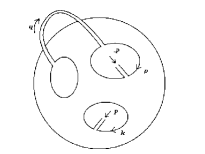
Figure 7: A genus 1 amplitude with 3 loops and 2 external legs

Performing the integration over the loop momenta one obtains the following function of the Schwinger parameters

$$I(\alpha,\beta,\gamma,\delta,\eta,\zeta;P)={\pi^{3d\over 2}\over\bigl{(}D+F\theta^{2}\bigr{)}^{d\over 2}}\,{\rm e}^{-P^{2}\theta^{2}{E+\theta^{2}\over D+F\theta^{2}}}$$ (78)

where

$$D\equiv(\alpha+\beta+\gamma)(\zeta\delta+\zeta\eta+\delta\eta)+\alpha\beta(\zeta+\eta)+$$

$$\qquad\,+\beta\gamma(\delta+\eta)+\gamma\alpha(\delta+\zeta)+\alpha\beta\gamma$$

$$E\equiv(\alpha+\eta)(\beta+\zeta)+\delta(\alpha+\beta+\zeta+\eta)$$

$$F\equiv\gamma+\eta+\zeta$$ (79)

If the function $g(\alpha,\beta,\gamma,\delta,\eta,\zeta)$ is sufficiently regular at infinity, we can replace in Eq. (B) the integral $I$ with its asymptotic expression for $\theta\to\infty$

$$I(\alpha,\beta,\gamma,\delta,\eta,\zeta;P)\,\mathrel{\mathop{\rightarrow}_{\theta\to\infty}}\,{\pi^{3d\over 2}\over F^{d\over 2}\theta^{d}}\,{\rm e}^{-{P^{2}\theta^{2}\over F}}$$ (80)

Note the $\theta$ dependence of this amplitude: first of all there is a multiplicative factor $1/\theta^{d}$, which in the general case becomes $1/\theta^{dg}$. The non-trivial dependence on the Schwinger parameters of the exponential factor ${\rm e}^{-{P^{2}\theta^{2}\over F}}$ is the source of the IR-UV mixing effect: if the external momenta are non-exceptional, $P\not=0$, the UV divergences at $F=0$ are regulated by the UV cut-off $1/(P\theta)$. This is what makes the limit $\theta\to\infty$ non-uniform in the external momenta.

Note that when the number $L$ of loop momenta equals $2g$ — and thus the number of faces of the higher genus diagram is 1 — the matrix $D_{AB}$ in Eq. (76) has maximal rank and, thus, in this case the Moyal factor regulates all the loop integrations. For this special kind of diagrams the analogue of the function $F$ appearing in (79) does not vanish for any value of the Schwinger parameters and hence there is no UV-IR mixing effect. For example consider the amplitude, given in Figure 8, of genus 1, 2 loops and 2 external legs carrying momentum $\pm P$:

$$\int\!\!d\alpha\,d\beta\,d\gamma\,f(\alpha,\beta,\gamma)\,\int\!d^{d}p\,d^{d}q\,{\rm e}^{-\bigl{[}\alpha p^{2}+\beta q^{2}+\gamma(p+q)^{2}+2ip\wedge q+2ip\wedge P\bigr{]}}$$

$$\qquad=\int\!\!d\alpha\,d\beta\,d\gamma\,f(\alpha,\beta,\gamma)\,{\pi^{d}\over\bigl{[}\alpha\beta+\alpha\gamma+\beta\gamma+\theta^{2}\bigr{]}^{d\over 2}}\,{\rm e}^{-{\theta^{2}\,P^{2}(\beta+\gamma)\over\alpha\beta+\alpha\gamma+\beta\gamma+\theta^{2}}}$$

$$\qquad\mathrel{\mathop{\rightarrow}_{\theta\to\infty}}\,{\pi^{d}\over\theta^{d}}\int\!\!d\alpha\,d\beta\,d\gamma\,f(\alpha,\beta,\gamma)\,{\rm e}^{-(\beta+\gamma)\,P^{2}}$$ (81)

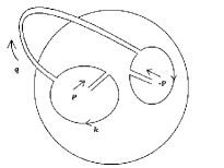
Figure 8: A genus 1 amplitude with 2 loops and 2 external legs

Summarizing, in the $\theta\to\infty$ limit, the integrated amplitudes go as $\theta^{-dg}$, while the non-integrated ones vanish exponentially. This is somewhat analogous to what happens in $N\times N$ matrix field theories, under the identification ${1\over N}\leftrightarrow{1\over\theta^{d}}$. In this analogy the contributions to the non-commutative amplitudes coming from non-exceptional external momenta correspond to the ${\rm e}^{-N}$ non-perturbative instanton effects of matrix theory.

Appendix C 1PI RG equation in the planar limit

In this appendix we derive the RG equation (5) satisfied by the generating functional of spherical 1PI amplitudes of a non-commutative scalar field theory. The derivation is done for $N\times N$ matrix field theory but the result also applies to the Moyal case.

Let $F_{\Lambda}[J]$ be the functional of the $N\times N$ matrix source $J(p)$ that generates connected amplitudes. $F_{\Lambda}[J]$ is related with the generating functional of connected and amputates amplitudes $H_{\Lambda}[\varphi]$ via

$$F_{\Lambda}[J]=H_{\Lambda}[\Delta_{\Lambda}\,J]+{1\over 2N}\int\!\!dp\,\Delta_{\Lambda}(p)\,{\rm Tr}\,J(p)\,J({\scriptstyle-}p)$$ (82)

and thus [4] it satisfies the following finite $N$ RG equation

$$\Lambda\partial_{\Lambda}\,F_{\Lambda}={1\over 2}\,\int\!\!dp\,\dot{\Delta}_{\Lambda}(p)\,\Delta_{\Lambda}^{-2}(p)\,\Bigl{[}N\,{\rm Tr}\,\Bigl{(}{\delta F_{\Lambda}\over\delta J(p)}\,{\delta F_{\Lambda}\over\delta J({\scriptstyle-}p)}\Bigr{)}$$

$$\qquad\qquad\qquad+{1\over N}\,{\rm Tr}\,{\delta^{2}F_{\Lambda}\over\delta J(p)\,\delta J({\scriptstyle-}p)}-\Delta_{\Lambda}(p)\Bigr{]}$$ (83)

The generating functional $\Gamma_{\Lambda}^{\prime}[\varphi]$ of 1PI amplitudes is the Legendre transform of $F_{\Lambda}[J]$:

$$\Gamma_{\Lambda}^{\prime}[\varphi]=\Gamma_{\Lambda}[\varphi]-{1\over 2N}\,\int\!\!dp\,\Delta^{-1}_{\Lambda}(p)\,{\rm Tr}\,\varphi(p)\,\varphi({\scriptstyle-}p)=$$

$$\qquad\,\,=F_{\Lambda}[J]-{1\over N}\,\int\!\!dp\,{\rm Tr}\,J(p)\,\varphi({\scriptstyle-}p)$$ (84)

where

$$\varphi_{\scriptscriptstyle ij}(p)=N\,{\delta F_{\Lambda}\over\delta J_{\scriptscriptstyle ji}({\scriptstyle-}p)}$$ (85)

By taking the $\Lambda$ derivative of $\Gamma_{\Lambda}[\varphi]$ and using Eq. (83), one finds

$$\!\!\!\!\!\!\!\!\Lambda\partial_{\Lambda}\,\Gamma_{\Lambda}=\Lambda\partial_{\Lambda}\,F_{\Lambda}-{1\over 2}\int\!\!dp\,\dot{\Delta}_{\Lambda}(p)\,\Delta^{-2}_{\Lambda}(p)\,{\rm Tr}\,\varphi(p)\,\varphi({\scriptstyle-}p)=$$

$$\qquad\,={1\over 2}\,\int\!\!dp\,\dot{\Delta}_{\Lambda}(p)\,\Delta_{\Lambda}^{-2}(p)\,\Bigl{[}{1\over N}\,{\rm Tr}\,{\delta^{2}F_{\Lambda}\over\delta J(p)\,\delta J({\scriptstyle-}p)}-\Delta_{\Lambda}(p)\Bigr{]}$$ (86)

Let us introduce the matrices

$$\Bigl{(}\mathbb{F}^{(2)}_{\Lambda}\Bigr{)}_{\scriptscriptstyle(i_{1}j_{1};\,p_{1}),(i_{2}j_{2};\,p_{2})}\equiv{\delta^{2}F_{\Lambda}\over\delta J_{\scriptscriptstyle i_{1}j_{1}}(p_{1})\,\delta J_{\scriptscriptstyle j_{2}i_{2}}({\scriptstyle-}p_{2})}$$

$$\Bigl{(}\mathbb{G}^{\prime\,(2)}_{\Lambda}\Bigr{)}_{\scriptscriptstyle(i_{1}j_{1};\,p_{1}),(i_{2}j_{2};\,p_{2})}\equiv{\delta^{2}\Gamma^{\prime}_{\Lambda}\over\delta\varphi_{\scriptscriptstyle i_{1}j_{1}}(p_{1})\,\delta\varphi_{\scriptscriptstyle j_{2}i_{2}}({\scriptstyle-}p_{2})}$$ (87)

whose row and column indices are given by the triples $(ij;\,p)$. Taking the $J$ derivative of Eq. (85) and the $\varphi$ derivative of (84) one obtains

$$\mathbb{F}^{(2)}_{\Lambda}\,\mathbb{G}^{\prime\,(2)}_{\Lambda}=\mathbb{I}$$ (88)

where, here and in the following, matrix multiplication involves both a sum over double indices $(ij)$ and an integral over momentum $p$; furthermore $\mathbb{I}\equiv\delta_{i_{1}i_{2}}\,\delta_{j_{1}j_{2}}\,\delta(p_{1}-p_{2})$. The result (88) together with (86) leads to the RG evolution equation for the 1PI generating functional at finite $N$:

$$\!\!\!\!\!\!\!\!\!\Lambda\partial_{\Lambda}\,\Gamma_{\Lambda}={1\over 2N^{2}}\,\mathbb{T}\mathrm{r}\,\Bigl{[}\dot{\mathbb{D}}_{\Lambda}\,\mathbb{D}_{\Lambda}^{-1}\,\Bigl{(}\mathbb{I}-N\,\mathbb{D}_{\Lambda}\,\mathbb{G}^{(2)}_{\Lambda}\Bigr{)}^{-1}\Bigr{]}-{1\over 2N^{2}}\,\mathbb{T}\mathrm{r}\,\dot{\mathbb{D}}_{\Lambda}\,\mathbb{D}_{\Lambda}^{-1}=$$

$$\qquad={1\over 2}\sum_{n=1}^{\infty}N^{n-2}\,\mathbb{T}\mathrm{r}\,\Bigl{[}\dot{\mathbb{D}}_{\Lambda}\,\mathbb{D}_{\Lambda}^{-1}\,\Bigl{(}\mathbb{D}_{\Lambda}\,\mathbb{G}^{(2)}_{\Lambda}\Bigr{)}^{n}\Bigr{]}$$ (89)

where

$$\bigl{(}\mathbb{D}_{\Lambda}\bigr{)}_{\scriptscriptstyle(i_{1}j_{1};\,p_{1}),(i_{2}j_{2};\,p_{2})}\equiv\Delta(p_{1})\,\delta_{i_{1}i_{2}}\,\delta_{j_{1}j_{2}}\,\delta(p_{1}-p_{2})$$ (90)

and $\mathbb{T}\mathrm{r}$ denotes the trace over the triple $(ij;\,p)$.

The large $N$ limit of Eq. (89) is defined by taking the invariants

$$\Omega_{k}(p_{1}\cdots p_{k})={1\over N}\,{\rm Tr}\Bigl{(}\varphi(p_{1})\cdots\varphi(p_{k})\Bigr{)}$$ (91)

fixed as $N\to\infty$. Hence one has to express derivatives with respect to $\varphi$ in terms of $\Omega_{k}$-derivatives:

$${\delta\Gamma_{\Lambda}\over\delta\varphi_{\scriptscriptstyle ij}(p)}={1\over N}\,\sum_{k}k\,\int\prod_{\alpha=1}^{k-1}dq_{\alpha}\,\bigl{(}\varphi(q_{1})\cdots\varphi(q_{k-1})\bigr{)}_{\scriptscriptstyle ji}\,{\delta\Gamma_{\Lambda}\over\delta\Omega_{k}(p,q_{1},\ldots,q_{k-1})}$$ (92)

and

$$\!\!\!\!\!\!{\delta^{2}\Gamma_{\Lambda}\over\delta\varphi_{\scriptscriptstyle i_{1}j_{1}}(p_{1})\,\delta\varphi_{\scriptscriptstyle j_{2}i_{2}}({\scriptstyle-}p_{2})}={1\over N}\sum_{k}\sum_{I=0}^{k-2}k\!\int\!\prod_{\alpha=1}^{k-2}dq_{\alpha}\,\bigl{(}\varphi(q_{1})\cdots\varphi(q_{I})\bigr{)}_{\scriptscriptstyle i_{2}i_{1}}\times$$ (93)

$$\qquad\times\bigl{(}\varphi(q_{I+1})\cdots\varphi(q_{k-2})\bigr{)}_{\scriptscriptstyle j_{1}j_{2}}\,{\delta\Gamma_{\Lambda}\over\delta\Omega_{k}(p_{1},q_{1},\ldots,q_{I},{\scriptstyle-}p_{2},q_{I+1},\ldots,q_{k-2})}+$$

$$\qquad+{1\over N^{2}}\,\sum_{k,k^{\prime}}k\,k^{\prime}\!\int\!\prod_{\alpha=1}^{k-1}dq_{\alpha}\!\!\prod_{\beta=1}^{k^{\prime}-1}dq^{\prime}_{\beta}\,\bigl{(}\varphi(q_{1})\cdots\varphi(q_{k-1})\bigr{)}_{\scriptscriptstyle j_{1}i_{1}}\times$$

$$\qquad\times\bigl{(}\varphi(q^{\prime}_{1})\cdots\varphi(q^{\prime}_{k^{\prime}-1})\bigr{)}_{\scriptscriptstyle i_{2}j_{2}}\,{\delta^{2}\Gamma_{\Lambda}\over\delta\Omega_{k}(p_{1},q_{1},\ldots,q_{k-1})\,\delta\Omega_{k^{\prime}}({\scriptstyle-}p_{2},q^{\prime}_{1},\ldots,q^{\prime}_{k-1})}$$

The second addendum in the R.H.S. of the equation above if of sub-leading order in $1/N$ and must be discarded in the large $N$ limit. Thus we find:

$$\!\!\!\!\!\!\!\!N^{n-2}\,\mathbb{T}\mathrm{r}\Bigr{(}\mathbb{G}^{(2)}_{\Lambda}\Bigr{)}^{n}=\int\!d{\rm P_{0}}\cdots d{\rm P_{n-1}}\,\prod_{i=1}^{n}\Biggl{[}\sum_{k_{i}}\sum_{I_{i}=0}^{k_{i}-2}\int\!\!\prod_{\alpha_{i}=1}^{I_{i}}\!\!dp^{(i)}_{\alpha_{i}}\!\!\prod_{\beta_{i}=1}^{k_{i}-2-I_{i}}\!\!dq^{(i)}_{\beta_{i}}\times$$ (94)

$$\quad\times\,k_{i}\,{\delta\Gamma_{\Lambda}\over\delta\Omega_{k_{i}}({\rm P_{i-1}},C_{i},{\scriptstyle-}{\rm P_{i}},C^{\prime}_{i})}\Biggr{]}\,\Omega_{\textstyle{\scriptscriptstyle\sum_{i}I_{i}}}(C_{n},\ldots,C_{1})\,\Omega_{\textstyle{\scriptscriptstyle\sum_{i}k_{i}-2-I_{i}}}(C^{\prime}_{1},\ldots,C^{\prime}_{n})$$

where $C_{i}\equiv\{p^{(i)}_{\alpha_{i}}\}$, $C^{\prime}_{i}\equiv\{q^{(i)}_{\beta_{i}}\}$. Using the identity (94) in the flow equation (89) we end up with the large $N$ (or large $\theta$) RG equation for the 1PI generating functional

$$\Lambda\partial_{\Lambda}\Gamma_{\Lambda}={1\over 2}\,\sum_{n=1}^{\infty}\int\!d{\rm P_{0}}\cdots d{\rm P_{n-1}}\,\dot{\Delta}_{\Lambda}({\rm P_{0}})\,\Delta_{\Lambda}({\rm P_{1}})\cdots\Delta_{\Lambda}({\rm P_{n-1}})\times$$

$$\qquad\times\prod_{i=1}^{n}\Biggl{[}\sum_{k_{i}}\sum_{I_{i}=0}^{k_{i}-2}\int\!\!\prod_{\alpha_{i}=1}^{I_{i}}\!\!dp^{(i)}_{\alpha_{i}}\!\!\prod_{\beta_{i}=1}^{k_{i}-2-I_{i}}\!\!dq^{(i)}_{\beta_{i}}\,k_{i}\,{\delta\Gamma_{\Lambda}\over\delta\Omega_{k_{i}}({\rm P_{i-1}},C_{i},{\scriptstyle-}{\rm P_{i}},C^{\prime}_{i})}\Biggr{]}\times$$

$$\qquad\times\,\Omega_{\textstyle{\scriptscriptstyle\sum_{i}I_{i}}}(C_{n},\ldots,C_{1})\,\Omega_{\textstyle{\scriptscriptstyle\sum_{i}k_{i}-2-I_{i}}}(C^{\prime}_{1},\ldots,C^{\prime}_{n})$$ (95)

which coincides with Eq. (5) of Section 2.