Who Confines Quarks?
- On Non-Abelian Monopoles and
Dynamics of Confinement

Abstract

The role non-Abelian magnetic monopoles play in the dynamics of confinement is discussed by examining carefully a class of supersymmetric gauge theories as theoretical laboratories. In particular, in the so-called $r$-vacua of softly broken ${N}=2$ supersymmmetric $SU(n_{c})$ QCD, the Goddard-Olive-Nuyts-Weinberg monopoles appear as the dominant low-energy effective degrees of freedom. Even more interesting is the physics of confining vacua which are deformations of nontrivial superconformal theories. We argue that in such cases, occurring in the $r={n_{f}\over 2}$ vacua of $SU(n_{c})$ theories or in all of confining vacua of $USp(2n_{c})$ or $SO(n_{f})$ theories with massless flavors, a new mechanism of confinement involving strongly interacting non-Abelian magnetic monopoles is at work.

1 Confinement as a dual superconductor?

The basic issue underlying the problem of confinement and dynamical symmetry breaking in QCD is the nature of the effective degrees of freedom and their interactions. The idea of Abelian gauge fixing and the resulting picture of (Abelian) dual superconductivity mechanism for confinement [1] implies that the most relevant low-energy effective degrees of freedom are the magnetic monopoles of two types, carrying each unit charge with respect to the two $U(1)$ subgroups of the color $SU(3)$ group. Condensation of these monopoles would lead to confinement of electric charges. This scenario, however, leaves many questions unanswered. One is the issue of chiral symmetry breaking. Do the Abelian monopoles carry flavor quantum numbers? If so, which, and how? Does confinement induce chiral symmetry breaking? Also, what is the gauge dependence of such a description?

Another, more serious problem is this. Does the Abelian dominance of confinement imply dynamical color $SU(3)\to U^{2}(1)$ breaking, with a characteristic enrichment of meson spectrum? There are no phenomenological indication that this takes place in the real world of strong interactions. If so, what are the other relevant degrees of freedom, and how do they interact? What is the structure of the low-energy effective action?

Lattice QCD has not given a clear answer to these questions so far.

Here we follow another approach: we examine carefully certain solvable models which are basically very similar to QCD but in which mechanism of confinement and dynamical flavor symmetry breaking can be studied in exact, quantum mechanical fashon [2]^-[9]. The models which we study with particular attention will be softly broken ${N}=2\,$ supersymmetric gauge theories with gauge groups $SU(n_{c})$, $USp(2n_{c})$ and $SO(n_{c})$, and with all possible numbers of fundamental quark flavors, compatible with asymptotic freedom [5]^-[9].

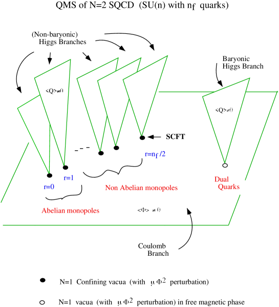
Figure 1: Quantum moduli space of $SU(n_{c})$ theories.

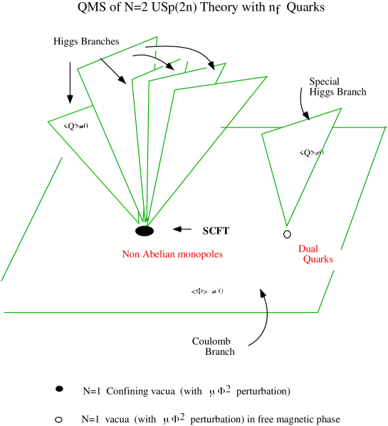
Figure 2: Quantum moduli space of $USp(2n_{c})$ theories.

1.1 Models and Global Symmetry

The Lagrangian has the structure

$${L}={1\over 8\pi}{\hbox{\rm Im}}\,\tau_{cl}\left[\int d^{4}\theta\,\Phi^{\dagger}e^{V}\Phi+\int d^{2}\theta\,{1\over 2}WW\right]+{L}^{(quarks)}+\Delta{L},$$ (1)

where

$$\Delta{L}=\int\,d^{2}\theta\,\,\mu\,{\hbox{\rm Tr}}\,\Phi^{2},\qquad\tau_{cl}\equiv{\theta_{0}\over\pi}+{8\pi i\over g_{0}^{2}}$$ (2)

and (${N=}2$) gauge multiplet $\Phi=\phi\,+\,\sqrt{2}\,\theta\,\psi+\,\ldots;$ $W_{\alpha}=-i\lambda\,+\,{i\over 2}\,(\sigma^{\mu}\,{\bar{\sigma}}^{\nu})_{\alpha}^{\beta}\,F_{\mu\nu}\,\theta_{\beta}+\,\ldots$ are both in the adjoint representation;

$${L}^{(quarks)}=\sum_{i}\,[\int d^{4}\theta\,\{Q_{i}^{\dagger}e^{V}Q_{i}+{\tilde{Q}_{i}}^{\dagger}e^{{\tilde{V}}}{\tilde{Q}}_{i}\}+\int d^{2}\theta\,\{\sqrt{2}{\tilde{Q}}_{i}\Phi Q^{i}+m_{i}{\tilde{Q}}_{i}Q^{i}\}]$$ (3)

describes the $n_{f}$ quarks and squarks.

The number of flavor is limited to

$$n_{f}\leq 2n_{c},\,\,2n_{c}+2,\,\,n_{c}-2,\qquad{\hbox{\rm for}}\quad SU(n_{c}),\,\,USp(2n_{c}),\,\,SO(n_{c}),$$

respectively, by the requirement of asymptotic freedom. The global symmetry of the model is ($m_{i}\to 0$):

$$G_{F}=\cases{U(n_{f})\times Z_{2n_{c}-n_{f}}\qquad SU(n_{c});\cr SO(2n_{f})\times Z_{2n_{c}+2-n_{f}}\qquad USp(2n_{c});\cr USp(2n_{f})\times Z_{2n_{c}-2n_{f}-4}\qquad SO(n_{c})}$$ (4)

It turns out that upon ${N}=1$ perturbation $\Delta{L}$, and with generic quark masses, only a discrete set of vacua remain. Most important of all, vacua in confinement phase can be classified further by the type of the low-energy degrees of freedom and by the way they interact. See Figs 1,2 and below.

1.2 Different types of Confining Vacua in Softly Broken ${N}=2$ Gauge Theories

Indeed, different types of confining vacua are [6] (see also Table 1.2):

1. Abelian dual superconductor - with dynamical Abelianization. The effective action has the form of a magnetic $U(1)^{R}$ gauge theory, where $R=$ rank of $G_{c}$.

   [Examples are: $r=0,1$ vacua in $SU(n_{c});$ also all vacua in theories with $n_{f}=0$];

2. Confinement by condensation of non-Abelian dual quarks of effective $SU(r)\times U(1)^{n_{c}-r+1}$ theory;

   [ $r=2,3,\ldots,[{n_{f}-1\over 2}]$ vacua of $SU(n_{c})$; also $USp(2n_{c}),SO(n_{c})$ models with $m\neq 0$ ]

3. Confining vacua which are deformed superconformal theories [ $r={n_{f}\over 2}$ vacua of $SU(n_{c})$; also all confining vacua in $USp(2n_{c}),SO(n_{c})$ models with $m=0$ ].

4. There exist also vacua in free-magnetic phase, with no confinement, no DSB, for theories with larger $n_{f}$ (e.g. $n_{f}\geq n_{c},$ in $SU(n_{c})$.)

We wish to find out:

Why does Abelianization occur in some vacua?

What are the dual quarks?

What degrees of freedom are there in SCFT and how do they interact?

Phases of $SU(n_{c})$ gauge theory with $n_{f}$ flavors. ${\tilde{n}}_{c}\equiv n_{f}-n_{c}$. NB and BR stand for the “non-baryonic” and “baryonic” Higgs branches. label ($r$) Deg.Freed. Eff. Gauge Group Phase Global Symmetry $0$ (NB) monopoles $U(1)^{n_{c}-1}$ Confinement $U(n_{f})$ $1$ (NB) monopoles $U(1)^{n_{c}-1}$ Confinement $U(n_{f}-1)\times U(1)$ $2,..,[{n_{f}-1\over 2}]$ (NB) dual quarks $SU(r)\times U(1)^{n_{c}-r}$ Confinement $U(n_{f}-r)\times U(r)$ ${n_{f}/2}$ (NB) rel. nonloc. - Almost SCFT $U({n_{f}/2})\times U({n_{f}/2})$ BR dual quarks $SU({\tilde{n}}_{c})\times U(1)^{n_{c}-{\tilde{n}}_{c}}$ Free Magnetic $U(n_{f})$

Phases of $USp(2n_{c})$ gauge theory with $n_{f}$ flavors with $m_{i}\to 0$. ${\tilde{n}}_{c}\equiv n_{f}-n_{c}-2$. label ($r$) Deg.Freed. Eff. Gauge Group Phase Global Symmetry 1st Group rel. nonloc. - Almost SCFT $U(n_{f})$ 2nd Group dual quarks $USp(2{\tilde{n}}_{c})\times U(1)^{n_{c}-{\tilde{n}}_{c}}$ Free Magnetic $SO(2n_{f})$

2 Non-Abelian Monopoles

2.1 Gauge Symmetry Breaking and Goddard-Nuyts-Olive-Weinberg monopoles

In order to answer these questions, let us first recall some well-known and some relatively little-known facts about non-Abelian monopoles [10, 7]. The relevant setting is a gauge theory in which gauge symmetry is broken spontaneously as

$$G\,\,\,{\stackrel{{\scriptstyle\langle\phi\rangle\neq 0}}{{\longrightarrow}}}\,\,\,H$$ (5)

where $H$ is in general non-Abelian. Finite energy classical configurations are such that

$${D}\phi\,\,\,{\stackrel{{\scriptstyle r\to\infty}}{{\longrightarrow}}}\,\,\,0,\quad\Rightarrow\quad\phi\sim U\cdot\langle\phi\rangle\cdot U^{-1}\sim\Pi_{2}(G/H)=\Pi_{1}(H)$$

$$A_{i}^{a}\sim U\cdot{\partial_{i}}U^{\dagger}\to\epsilon_{aij}{r_{j}\over r^{3}}G(r):$$ (6)

they represent elements of the homotopy group $\Pi_{1}(H).$ Asymptotically we can take

$$G(r)=\beta_{i}T_{i},\qquad T_{i}\in{\hbox{\rm Cartan S.A. of }}\,\,\,H$$ (7)

so that the constant vectors $\beta_{i}$ characterize the configurations.

Topological quantization leads to the result that

$$\beta_{i}={\hbox{\rm weight vectors of}}\,\,{\tilde{H}}={\hbox{\rm dual of}}\,\,H,$$

where examples of duals of gauge groups are:

$${\tilde{H}}\Leftrightarrow H$$

$SU(N)/Z_{N}$	$\Leftrightarrow$	$SU(N)$
$SO(2N)$	$\Leftrightarrow$	$SO(2N)$
$SO(2N+1)$	$\Leftrightarrow$	$USp(2N)$

Note that as $|\phi|\to\infty$ these finite energy solutions become singular Dirac type monopoles. Also, in the simplest case of $G=SU(2)$, $H=U(1)$ they reduce to the well known ’t Hooft-Polyakov monopoles.

2.2 Quantum Numbers of N.A. monopoles

In order to see what quantum numbers these monopoles carry, let us consider first the simplest case

$$SU(3){\stackrel{{\scriptstyle\langle\phi\rangle}}{{\longrightarrow}}}SU(2)\times U(1),\qquad\langle\phi\rangle=\pmatrix{v&0&0\cr 0&v&0\cr 0&0&-2v}$$

Consider the subgroup $SU_{U}(2)\subset SU(3)$

$$t^{4}={1\over 2}\pmatrix{0&0&1\cr 0&0&0\cr 1&0&0};\quad t^{5}={1\over 2}\pmatrix{0&0&-i\cr 0&0&0\cr i&0&0};\quad{t^{3}+\sqrt{3}t^{8}\over 2}={1\over 2}\pmatrix{1&0&0\cr 0&0&0\cr 0&0&-1};\quad$$

which is broken as

$$SU_{U}(2){\stackrel{{\scriptstyle\langle\phi\rangle}}{{\longrightarrow}}}U_{U}(1).$$

Use ’t Hooft-Polyakov solution for $\phi(r),A(r)$ for the broken $SU_{U}(2)$, one finds a $SU(3)$ solution (Sol. 1) :

$$\phi=\left(\begin{array}[]{ccc}-\frac{1}{2}v&0&0\\ 0&v&0\\ 0&0&-\frac{1}{2}v\\ \end{array}\right)+\frac{3}{2}v\Big{(}t_{4},t_{5},\frac{t_{3}}{2}+\frac{\sqrt{3}t_{8}}{2}\Big{)}\cdot\hat{r}\phi(r),$$

$$\vec{A}=\Big{(}t_{4},t_{5},\frac{t_{3}}{2}+\frac{\sqrt{3}t_{8}}{2}\Big{)}\wedge\hat{r}A(r).\qquad$$ (8)

Another solution (Sol. 2) can be found by considering another $SU_{V}(2)\subset SU(3)$

$$t^{6}={1\over 2}\pmatrix{0&0&0\cr 0&0&1\cr 0&1&0};\quad t^{7}={1\over 2}\pmatrix{0&0&0\cr 0&0&-i\cr 0&i&0};\quad{-t^{3}+\sqrt{3}t^{8}\over 2}={1\over 2}\pmatrix{0&0&0\cr 0&1&0\cr 0&0&-1},\quad$$

leading to a degenerate doublet of monopoles with charges.

monopoles	${\tilde{SU}(2)}$	${\tilde{U}(1)}$
${\tilde{q}}$	${\underline{2}}$	$1$

2.3 Generalization

Generalization to the case of the symmetry breaking

$$SU(n){\stackrel{{\scriptstyle\langle\phi\rangle}}{{\longrightarrow}}}SU(r)\times U^{n-r}(1),\qquad\langle\phi\rangle=\pmatrix{v_{1}{\bf 1}_{r\times r}&{\bf 0}&\ldots&{\bf 0}\cr{\bf 0}&v_{2}&0&\ldots\cr{\bf 0}&0&\ddots&\ldots\cr{\bf 0}&0&\ldots&v_{n-r+1}}$$

can be done by considering various $SU_{i}(2)$ subgroups ($i=1,2,\ldots,r$) living in $[i,r+1]$ subspace: one finds (see the Table below)

Degenerate $r$-plet of monopoles ($q$);

Also, Abelian monopoles ($e_{i}$), ($i=1,2,\ldots,n-r-1$) of $U^{n-r-1}(1)$ (non degenerate) appear;

monopoles	${\tilde{SU}}(r)$	${\tilde{U}_{0}(1)}$	${\tilde{U}_{1}(1)}$	${\tilde{U}_{2}(1)}$	$\ldots$	${\tilde{U}_{n-r-1}(1)}$
$q$	${\underline{r}}$	$1$	$0$	$0$	…	$0$
${e}_{1}$	${\underline{1}}$	$0$	$1$	$0$	$\ldots$	$0$
${e}_{2}$	${\underline{1}}$	$0$	$0$	$1$	$0$	$0$
$\vdots$	${\underline{1}}$	$0$	$\ldots$			$0$
${e}_{n-r-1}$	${\underline{1}}$	$0$	$0$	$\ldots$	$\ldots$	$1$

These monopoles have the same charge structures found in the $\,r\,$-vacua of ${N}=2$ SQCD (!)

Also, the flavor quantum numbers of non-Abelian monopoles can be understood by the generalized Jackiw-Rebbi mechanism[7].

2.4 Subtleties

There are certain subtleties around the non-Abelian monopoles:

“Colored dyons” have been shown not to exist.[8] Actually there is no paradox here. Non-Abelian monopoles carry both Abelian and non-Abelian charges, but both refer to ${\tilde{H}},$ not $H$ itself, while the results of Abouelsaood et.al. [8] refer to a non-Abelian generalization of charge fractionalization, which is not possible;

Non-Abelian monopoles are to transform as members of various multiplets of the dual group ${\tilde{H}}$, not of $H$ itself. Any search for the “gauge zero modes” should involve non-local field transformations;

It is not justified to study the system

$$G\,\,\,{\stackrel{{\scriptstyle\langle\phi\rangle\neq 0}}{{\longrightarrow}}}\,\,\,H$$

as a limit of maximally broken cases ($H_{0}\subset$ Cartan S.A. of $G$):

$$\langle\phi\rangle={\bf h}\cdot{\bf H_{0}},\qquad h_{i}\to 0,\quad{\hbox{\rm for}}\quad H_{0i}\subset H.$$

To do so would necessarily lead one to the (non-semi-classical) domain of strongly coupled, infinitely extended, light monopoles (just think of taking the limit $v\to 0\,\,$ to study the ’t Hooft-Polyakov monopole of $\,\,\,SU(2)\,\,\,{\stackrel{{\scriptstyle v}}{{\longrightarrow}}}\,\,\,U(1)$ theory!).

Indeed, non-Abelian monopoles are never really semi-classical, even when

$$\langle\phi\rangle\gg\Lambda_{H},$$

if $H$ interactions grow strong in the IR: $H$ may be further dynamically broken at $\mu\sim\Lambda_{H}$. If it is, “non-Abelian monopoles” simply means a set of approximately degenerate monopoles .

Only if $H$ remains unbroken do non-Abelian monopoles in an irreducible representation of ${\tilde{H}}$ make appearance in the low-energy action.

Most remarkably, this last option seems to be realized in the $r$-vacua of $SU(n_{c})$, $n_{f}$ theories. We propose that the dual quarks are nothing but the GNO monopoles.

2.5 Duality

Further justification of our ideas comes from the duality considerations.

• $r$ vacua with $SU(r)\times U(1)^{n_{c}-r+1}$ gauge group occur only for

  $$r<{n_{f}\over 2}.$$

  This can be understood as due to the sign-flip of the beta function:

  $$b_{0}^{(dual)}\propto-2\,r+n_{f}>0,\qquad b_{0}\propto-2\,n_{c}+n_{f}<0,$$ (9)

  so that the low energy $SU(r)$ interactions are infrared-free. Note that for this to happen the flavor-dressing of the monopoles is essential.

• When this sign flip is not possible for some reason, such as in pure ${N}=2$ YM or in generic points of QMS of ${N}=2$ theories, dynamical Abelianization occurs.

• These questions are related to the resolution of the old Dirac-quantization-vs-Renormalization-Group puzzle (i.e., why the quantization condition

  $$g_{e}(\mu)\cdot g_{m}(\mu)=2\pi n,\qquad\forall\mu$$

  is valid at any scale $\mu$?) in the Seiberg-Witten model.

• The boundary, $r={n_{f}\over 2}$ case, is a SCFT (nontrivial IR fixed point): non-Abelian monopoles and dyons still show up as recognizable low-energy effective degrees of freedom, although their interactions are nonlocal.

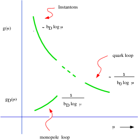
Figure 3: Duality. Monopole loop is equivalent to infinite instanton sum.

2.6 Dynamical Symmetry Breaking: a Puzzle

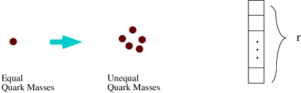
Figure 4:

• As the quark masses are chosen unequal, $m_{i}\neq m_{j}$, each of $r$ vacua splits into ${n_{f}\choose r}$ points in QMS. This is very suggestive of a possibility that the massless monopoles in each vacuum is an (Abelian) monopole in ${\underline{n_{f}\choose r}}$ representation of the global $SU(n_{f})$. This is precisely what happens in the $SU(2)$ theory with $n_{f}=1,2,3$. This would however (for generic $SU(n_{c})$ theories) lead to an effective action with an accidental global $SU({n_{f}\choose r})$ symmetry and hence to an enormous number of Nambu-Golstone bosons when these field condense.

• Actually this does not happen. The system avoids this awkward situation by having non-Abelian monopoles in ${\underline{r}}$ of dual color $SU(r)$, and in the fundamental representation ${\underline{n_{f}}}$ of the global $SU(n_{f})$. They condense [6] in color-flavor diagonal fashion

  $$\langle q_{\alpha}^{i}\rangle=\delta_{\alpha}^{i}\,v,\qquad\alpha=1,2,\ldots,r,\quad i=1,2,\ldots n_{f}$$ (10)

  (“Color-Flavor-Locking”), breaking the global symmetry as

  $$G_{F}=SU(N_{f})\times U(1)\Rightarrow U(r)\times U(n_{f}-r).$$ (11)

• The non-Abelian monopoles may be regarded as baryonic constituents of the Abelian monopole,

  $$U(1)\,{\hbox{\rm monopole}}\sim\epsilon^{a_{1}\ldots a_{r}}{q_{a_{1}}^{i_{1}}q_{a_{2}}^{i_{2}}\ldots q_{a_{r}}^{i_{r}}}.$$

  The Abelian monopole, $SU(r)$ being infrared free, breaks up into the former!

3 Almost Superconformal Confining Vacua

The most interesting sort of confining vacua we encounter in the softly broken ${N}=2$ supersymmetric gauge theories are however those which appear as deformation (perturbation) of a nontrivial superconformal theory [11, 12, 13]. In order to be concrete, let us study the case of the sextet vacua in $SU(3)$, $n_{f}=4$ (${N}=2$) supersymmetric QCD in some detail below [9].

3.1 Sextet Vacua of $SU(3)$, $n_{f}=4$ Model

The Seiberg-Witten curve of this theory equal bare quark masses ($m_{a}=m$) is [4]

$$y^{2}=\prod_{i=1}^{3}(x-\phi_{i})^{2}-(x+m)^{4}\equiv(x^{3}-Ux-V)^{2}-(x+m)^{4}.$$

At the sextet vacua of our interest ($diag\,\phi=(-m,-m,2m)$), $U=\langle{\hbox{\rm Tr }}\Phi^{2}\rangle={3\,m^{2}},\,\,$ $V=\langle{\hbox{\rm Tr }}\Phi^{3}\rangle=2\,m^{3},$ the curve exhibits a singular behavior, $y^{2}\propto(x+m)^{4}$ corresponding to the unbroken $SU(2)$ symmetry.

The well known mass formula is

$$M_{(g_{1},g_{2};q_{1},q_{2})}=\sqrt{2}\,|g_{1}\,a_{D1}+g_{2}\,a_{D2}+q_{1}\,a_{1}+q_{2}\,a_{2}|,$$

$$a_{D1}=\oint_{\alpha_{1}}\lambda,\qquad a_{D2}=\oint_{\alpha_{2}}\lambda,\qquad a_{1}=\oint_{\beta_{1}}\lambda,\qquad a_{2}=\oint_{\beta_{2}}\lambda,$$

where the (meromorphic) one-form $\lambda$ is given by

$$\lambda={x\over 2\pi}d\,\log{\prod(x-\phi_{i})-y\over\prod(x-\phi_{i})+y}.$$

3.2 Expansion near the SCFT Point

In order to find out the nature of the low-energy massless fields present, one has to expand around the singularity,

$$U={3m^{2}}+u,\qquad V=2m^{3}+v.$$

The discriminant of the curve factorizes as [13]

$$\Delta=\Delta_{s}\,\Delta_{+}\,\Delta_{-},\qquad\Delta_{s}=(m\,u-v)^{4}$$

so the loci of $\Delta=0$ are

$$v=m\,u,\qquad v=m\,u+\frac{u^{2}}{4},\qquad v=m\,u-\frac{u^{2}}{4}.$$

By rescaling    $u=m\,{\tilde{u}},\,\,v=m^{2}\,{\tilde{v}}$, and intersecting them with a $S^{3}$

$$|{\tilde{u}}|^{2}+|{\tilde{v}}|^{2}=1.$$

and making a stereographic projection from $S^{3}\to R^{3}$, one finds that the curves (in $u,v$ space) along which some particles become massless take the form of the three linked rings (Fig. 5).

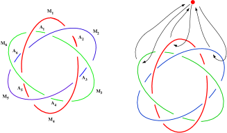
Figure 5: Loci in $u,v$ space where certain particles become massless.

3.3 Monodromy and Charges

In order to find what charges are carried by these massless particles, one has then to study the monodromy transformations (among $a_{D1},\,a_{D2},\,a_{1},\,a_{2}$) as one moves along various closed curves encircling parts of the linked rings.

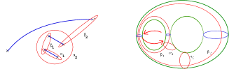
Figure 6: Homology cycles and the transformation exchanging the two necks of the bitorus.

For instance the monodromy around $M_{1}$ leads to

$$\alpha_{1}\to\alpha_{1},\qquad\beta_{1}\to\beta_{1}-4\alpha_{1},\qquad\alpha_{2}\to\alpha_{2},\qquad\beta_{2}\to\beta_{2}.$$

namely,

$$\pmatrix{a_{D1}\cr a_{D2}\cr a_{1}\cr a_{2}}\to M_{1}\pmatrix{a_{D1}\cr a_{D2}\cr a_{1}\cr a_{2}},\qquad M_{1}={\tilde{M}}_{1}^{4},\quad\,{\tilde{M}}_{1}=\pmatrix{1&0&0&0\cr 0&1&0&0\cr-1&0&1&0\cr 0&0&0&1}$$ (12)

From the formula

$$M=\pmatrix{{\bf 1}+{\vec{q}}\otimes{\vec{g}}&{\vec{q}}\otimes{\vec{q}}\cr-{\vec{g}}\otimes{\vec{g}}&{\bf 1}-{\vec{g}}\otimes{\vec{q}}}$$ (13)

the (four) massless particles at the singularity ${\tilde{v}}={\tilde{u}}$ are found to carry charges

$$(g_{1},g_{2};q_{1},q_{2})=(1,0;0,0),$$

i.e., they are four magnetic monopoles carrying the unit charge with respect to the first $U(1)$. Analogously:

$$M_{2}=\pmatrix{-1&0&1&0\cr 0&1&0&0\cr-4&0&3&0\cr 0&0&0&1},\qquad M_{6}=\pmatrix{1&1&1&0\cr 0&1&0&0\cr 0&0&1&0\cr 0&-1&-1&1},\quad etc.$$

By using then the conjugation relations among the monodromy matrices

$$M_{1}=M_{6}^{-1}A_{5}M_{6},\quad A_{2}=M_{2}^{-1}M_{1}M_{2},\quad M_{4}=M_{3}^{-1}A_{2}M_{3},\quad A_{5}=M_{5}^{-1}M_{4}M_{5},$$

$$M_{2}=M_{1}^{-1}A_{6}M_{1},\quad A_{3}=M_{3}^{-1}M_{2}M_{3},\quad M_{5}=M_{4}^{-1}A_{3}M_{4},\quad A_{6}=M_{6}^{-1}M_{5}M_{6},$$

$$M_{3}=M_{2}^{-1}A_{1}M_{2},\quad A_{4}=M_{4}^{-1}M_{3}M_{4},\quad M_{6}=M_{5}^{-1}A_{4}M_{5},\quad A_{1}=M_{1}^{-1}M_{6}M_{1}$$

they can be uniquely determined. They correspond to the charges

$$M_{1}:\,(1,0;0,0)^{4},\quad M_{4}:\,\,(-1,1;0,0)^{4},\quad M_{2}:\,(-2,0;1,0),\quad M_{5}:\,\,(2,-2;-1,0),$$

$$A_{2}:\,\,(-1,0;1,0)^{4},\quad A_{5}:\,\,(1,-1;-1,0)^{4},\quad A_{3}:\,\,(-2,2;-1,0),\quad A_{6}:\,\,(2,0;1,0),$$

$$M_{3}:\,(0,1;-1,0),\quad M_{6}:\,\,(0,1;1,0),\quad A_{4}:\,\,(4,-3;-1,0),\quad A_{1}:\,\,(-4,1;1,0).$$

Now

1. How are these $U(1)$ charges related to $SU(2)\times U(1)$ ?

2. Which of them are actually there at the SCFT Point?

3. How do they give $\beta=0$ ?

4. How do they interact ?

The first of these questions can be answered by studying the effect of transformation which exchanges the two necks of the bi-torus (Fig. 6),

$$\alpha_{1}\to\alpha_{2}-\alpha_{1};\qquad\beta_{1}\to-\beta_{1};\qquad\alpha_{2}\to\alpha_{2};\qquad\beta_{2}\to\beta_{1}+\beta_{2}.$$

This allows us to introduce a new basis such that one of the $U(1)$ factors is a subgroup of $SU(2)$ and another is orthogonal to it. In the new basis, the charges look as in Table 3.3.

Matrix	Charge
$M_{1},M_{4}$	$(\pm 1,1,0,0)^{4}$
$A_{2},A_{5}$	$(\pm 1,-1,\mp 1,0)^{4}$
$M_{2},M_{5}$	$(\pm 2,2,\mp 1,0)$
$A_{3},A_{6}$	$(\pm 2,-2,\pm 1,0)$
$M_{3},M_{6}$	$(0,2,\pm 1,0)$
$A_{1},A_{4}$	$(\pm 4,-2,\mp 1,0)$

3.4 Superconformal Limit ( $u=v=0$ )

We must first of all define SCFT limit appropriately.

• As $u,v\to 0$, the bitorus degenerates. If the branch points $\{b,c,d,e,f,g\}$ collapse to $(a,a,a,0,1,\infty)$ then $\tau$ becomes diagonal with (Lebowitz [14])

  $$a={{{\vartheta}_{3}}^{4}(0\,|\tau_{22})\over{{\vartheta}_{2}}^{4}(0\,|\tau_{22})};\qquad\frac{c-b}{d-b}={{{\vartheta}_{3}}^{4}(0\,|\tau_{11})\over{{\vartheta}_{2}}^{4}(0\,|\tau_{11})}.$$

• In our sextet vacua the curve has the singular form

  $$y^{2}=(x^{3}-ux-v)^{2}-x^{4}\to x^{4}(x+1)(x-1).$$

  By an apporpriate change of the variable $x$, one finds for the modular parameter of the large torus: $\tau_{22}\to 1$ (weakly interacting $U(1)$ theory);

• As for the small torus ( $SU(2)$ ), $\tau_{11}$ apparently depends on the way $u,\,v$ are taken to $0$.

• By studying the simplified curve $(x^{2}-ux-v)(x^{2}+ux+v)=0$ with variable change,

  $$v=\epsilon^{2};\qquad u=\epsilon\rho;\qquad x=\epsilon z;\qquad y=\epsilon^{2}w,$$

  one finds that $\tau_{11}$ depends only on $\rho.$

• In other words, different sections of the linked rings at different phase of $\epsilon$ are different ($SU(2,Z)$-related) descriptions of the same physics!

Thus we define the SCFT by taking the limit $\quad\epsilon\to 0,\quad\rho\to 0,$ namely, $\rho\to 0$ first. This finally yields the following charges of the massless particles in different sections. Note the three-fold periodicity.

$+2i$	$(0,1)$	$(4,-1)$	$(0,1)$	$(0,-1)$	$(-4,1)$	$(0,-1)$	$\ldots$
$2$	$(2,1)$	$(2,-1)$	$(2,-1)$	$(-2,-1)$	$(-2,1)$	$(-2,1)$	$\ldots$
$-2i$	$(0,-1)$	$(-4,1)$	$(0,-1)$	$(0,1)$	$(4,-1)$	$(0,1)$	$\ldots$
$-2$	$(-2,-1)$	$(-2,1)$	$(-2,1)$	$(2,1)$	$(2,-1)$	$(2,-1)$	$\ldots$
$\infty$	$(\pm 1,0)^{4}$	$(\mp 1,0)^{4}$	$(\pm 1,\mp 1)^{4}$	$(\mp 1,0)^{4}$	$(\pm 1,0)^{4}$	$(\mp 1,\pm 1)^{4}$	$\ldots$

1. The three sections are related by unimodular transformations 2

   $$p_{1}=\pmatrix{-1&4\cr 0&-1};\qquad p_{2}=\pmatrix{-1&-4\cr 1&3};\qquad p_{3}=\pmatrix{1&0\cr 1&1}.$$

2. At $\rho=0$, the small branch points are at $(2i,\,-2i,\,2,\,-2)$ so that one finds for $\tau_{11}$

   $${1\over 2}={{{\vartheta}_{3}}^{4}(0\,|\tau_{11})\over{{\vartheta}_{2}}^{4}(0\,|\tau_{11})},$$

   which has solutions

   $$\tau_{11}=\frac{\pm 1+i}{2},\qquad\frac{\pm 3+i}{10},\qquad\ldots$$

   Other solutions by $SL(2,Z)$ transformations $\tau\to\tau+2;\,\,\tau\to{\tau\over 1-2\tau}.$

3.5 Renormalization-Group Fixed Point

Now how do these massless particles give a vanishing beta function? In the case of a nontrivial $U(1)$ IR fixed point of the pure ${N}=2,$ $SU(3)$ Yang-Mills theory, cancellation occurs among a monopole, a dyon and an electron[11] (see Figure above).

The cancellation of $b_{0}$ in our case (consider $U_{1}(1)\subset SU(2)$) is more involved since now there are also contributions of the gauge multiplet. Nonetheless,

1. four monopole doublets $(\mp 1,0)^{4}$ cancel the contribution of the gauge multiplets;

2. a dyon doublet $(\pm 2,\pm 1)$ and an electric doublet $(0,\pm 1)$ cancel each other as

   $$\sum_{i}(q_{i}+m_{i}\tau)^{2}=1+(2\,\tau+1)^{2}=0,\qquad{\hbox{\rm for }}\quad\tau^{*}=\frac{-1+i}{2}:$$

   showing a nice (non-Abelian) generalization of Argyres-Douglas’ mechanism;

3. in the second section cancellation occurs because both the charges and the coupling constant $\tau^{*}$ get transformed by $p_{1}=\pmatrix{-1&4\cr 0&-1}$, and the above argument works for $(\pm 4,\mp 1)$ and $(\pm 2,\mp 1)$ with $\tau^{*}={3+i\over 10}$! This strengthens our idea that different sections are simply different descriptions of the same physics.

Thus the low-energy theory is an interacting SCFT with $SU(2)\times U(1)$ gauge group and four magnetic monopole doublets, one dyon doublet and one electric doublet.

3.6 Six Colliding ${N}=1$ Local Vacua:

Another way to study our SCFT would be to consider first the theory with unequal quark masses and then to take the limit of the equal mass. The SCFT singularity splits to six singularities.

• Each of the six ${N}=1$ theories is a local $U(1)^{2}$ theory with a pair of massless Abelian monopoles $M_{i},{\tilde{M}}_{i},$ ($i=1,2$) carrying each unit charge with respect to one of the $U(1)$ factors; altogether there are 12 massless hypermultiplets (as in the SCFT);

• The effect of ${N}=1$ perturbation $\mu\,{\hbox{\rm Tr}}\,\Phi^{2}$ can be studied in a well-known way, in terms of an effective superpotential:

  $${P}=\sum_{i=1}^{2}\sqrt{2}\,A_{D_{i}}\,M_{i}{\tilde{M}}_{i}+\mu\,U(A_{D1},A_{D2})+{\hbox{\rm mass terms }}$$ (14)

  which leads to $\langle M_{i}\rangle\neq 0$, $\langle{\tilde{M}}_{i}\rangle\neq 0$ (Confinement);

• However, in the $m_{i}\to m$ (SCFT) limit, the VEVS of the Abelian monopoles are found to vanish:

  $$\langle M_{i}\rangle\to 0,\quad\langle{\tilde{M}}_{i}\rangle\to 0.$$

  Analogous phenomenon was found in $SU(2)$, $n_{f}=1$ theory [15].

• We do know (from the large $\mu$ analysis, vacuum counting, and holomorphic dependence of physic on $\mu$) [6] however that the flavor group is dynamically broken in the perturbed SCFT vacua:

  $$G_{F}=SU(4)\times U(1)\Rightarrow U(2)\times U(2);$$ (15)

  then what is the order parameter of the symmetry breaking?

We propose that condensation of $SU(2)$ doublets ${M}_{\alpha}^{i},$ ($\alpha=1,2$, $\,i=1,\ldots,4$)

$$\langle{M}_{\alpha}^{i}\,{M}_{\beta}^{j}\rangle=\epsilon_{\alpha\beta}\,C^{ij}\neq 0,$$ (16)

is formed due to the strong $SU(2)$ interactions. This is compatible with the known dynamical symmetry breaking pattern. Note that, in the sense of complementarity, such VEVS can alternatively be understood as

$$\langle{M}_{\alpha}^{i}\rangle=\delta_{\alpha}^{i}\,v\neq 0$$

i.e., color-flavor diagonal VEVS as in the generic $r$-vacua.

3.7 Summary

Softly broken ${N}=2,$ $SU(n_{c})$ gauge theories with $n_{f}$ quarks thus exhibit various confining vacua with:

• physics quite different for

  (i) $r=0,1$ $\Rightarrow$ Weakly coupled Abelian monopoles;

  (ii) $r<{n_{f}\over 2}$ $\Rightarrow$ Weakly coupled non-Abelian monopoles;

  (iii) $r={n_{f}\over 2}$ $\Rightarrow$ Strongly coupled non-Abelian monopoles;

• nonetheless, both at generic $r$ - vacua and at the SCFT ($r={n_{f}\over 2}$) vacua, the non-Abelian monopoles condense as

  $$\langle{M}_{\alpha}^{i}\rangle=\delta_{\alpha}^{i}\,v\neq 0,\qquad(\alpha=1,2,\ldots,r;\quad i=1,2,\ldots,n_{f})$$

  (“Color-Flavor-Locking”);

• Abelian and non-Abelian monopoles apear to be related as

  $$\epsilon^{{\alpha_{1}}{\alpha_{2}}\ldots{\alpha_{r}}}{M}_{\alpha_{1}}^{i_{1}}{M}_{\alpha_{2}}^{i_{2}}\ldots{M}_{\alpha_{r}}^{i_{r}}\sim``U(1)"{\hbox{\rm monopole}}.$$

4 QCD

Finally let us come back briefly to the real-world QCD. Here

1. no dynamical Abelianization is known to occur;

2. on the other hand, in QCD with $n_{f}$ flavor, the original and dual beta functions have the first coefficients ($n_{c}=3$, ${\tilde{n}}_{c}=2,3$)

   $$b_{0}=-11\,n_{c}+2\,n_{f}\quad{\hbox{\rm vs}}\quad{\tilde{b}}_{0}=-11\,{\tilde{n}}_{c}+n_{f}:$$

   they have the same sign because of the large coefficient in front of the color multiplicity (cfr. Eq.(9)).

Barring that higher loops change the situation, this leaves us with the option of strongly-interacting non-Abelian monopoles. Is it possible that non-Abelian monopoles (perhaps certain composite theirof) carrying nontrivial flavor $SU_{L}(n_{f})\times SU_{R}(n_{f})$ quantum numbers condense yielding the global symmetry breaking such as

$$G_{F}=SU_{L}(n_{f})\times SU_{R}(n_{f})\Rightarrow SU_{V}(3),$$

observed in Nature? Are ’t Hooft’s Abelian monopoles in some sense composites of these non-Abelian monopoles ?

References

- [1] G. ’t Hooft, Nucl. Phys. B190 (1981) 455; S. Mandelstam, Phys. Lett. 53B (1975) 476.
- [2] N. Seiberg and E. Witten, Nucl. Phys. B426 (1994) 19; Erratum ibid. Nucl.Phys. B430 (1994) 485, hep-th/9407087.
- [3] N. Seiberg and E. Witten, Nucl. Phys. B431 (1994) 484, hep-th/9408099.
- [4] P. C. Argyres and A. F. Faraggi, Phys. Rev. Lett 74 (1995) 3931, hep-th/9411047; A. Klemm, W. Lerche, S. Theisen and S. Yankielowicz, Phys. Lett. B344 (1995) 169, hep-th/9411048; Int. J. Mod. Phys. A11 (1996) 1929, hep-th/9505150; A. Hanany and Y. Oz, Nucl. Phys. B452 (1995) 283, hep-th/9505075; P. C. Argyres, M. R. Plesser and A. D. Shapere, Phys. Rev. Lett. 75 (1995) 1699, hep-th/9505100; P. C. Argyres and A. D. Shapere, Nucl. Phys. B461 (1996) 437, hep-th/9509175; A. Hanany, Nucl.Phys. B466 (1996) 85, hep-th/9509176.
- [5] P. C. Argyres, M. R. Plesser and N. Seiberg, Nucl. Phys. B471 (1996) 159, hep-th/9603042.
- [6] G. Carlino, K. Konishi and H. Murayama, Nucl. Phys. B590 (2000) 37, hep-th/0005076; G. Carlino, K. Konishi, P. S. Kumar and H. Murayama, hep-th/0104064, Nucl. Phys. B608 (2001) 51.
- [7] S. Bolognesi and K. Konishi, Nucl. Phys. B645 (2002) 337, hep-th/0207161.
- [8] A. Abouelsaood, Nucl. Phys. B226 (1983) 309; P. Nelson and A. Manohar, Phys. Rev. Lett. 50 (1983) 943; A. Balachandran et. al., Phys. Rev. Lett. 50 (1983) 1553; P. Nelson and S. Coleman, Nucl. Phys. B227 (1984) 1; E. Weinberg, Phys.Rev.D54 (1996) 6351, hep-th/9605229.
- [9] R. Auzzi, R. Grena and K. Konishi, Nucl. Phys. B653 (2003) 204, hep-th/0211282.
- [10] P. Goddard, J. Nuyts and D. Olive, Nucl. Phys. B125 (1977) 1, E. Weinberg, Nucl. Phys. B167 (1980) 500; Nucl. Phys. B203 (1982) 445.
- [11] P. C. Argyres and M. R. Douglas, Nucl. Phys. B448 (1995) 93, hep-th/9505062.
- [12] P. C. Argyres, M. R. Plesser, N. Seiberg and E. Witten, Nucl. Phys. 461 (1996) 71, hep-th/9511154.
- [13] T. Eguchi, K. Hori, K. Ito and S.-K. Yang, Nucl. Phys. B471 (1996) 430, hep-th/9603002.
- [14] A. Lebowitz, Israel J. Math. 12 (1972) 223.
- [15] A. Gorsky, A. Vainshtein and A. Yung, Nucl. Phys. B584 (2000) 197, hep-th/0004087.