A comprehensive introduction to logarithmic conformal field theory, using an algebraic point of view, is given. A number of examples are explained in detail, including the $c=-2$ triplet theory and the $k=-4/3$ affine $su(2)$ theory. We also give some brief introduction to the work of Zhu.

1 Introduction

In the last few years conformal field theories whose correlation functions have logarithmic branch cuts have attracted some attention. The interest in these logarithmic conformal field theories has been motivated from two different points of view. First of all, models with this property seem to play an important role for the description of certain statistical models, in particular in the theory of (multi)critical polymers [1, 2, 3], percolation [4], two-dimensional turbulence [5, 6, 7], the quantum Hall effect [8, 9], the sandpile model [10] and disordered systems [11, 12, 13, 14, 15, 16]. Secondly, this new class of conformal field theories is of conceptual interest since it is likely to shed light on the structure of more general conformal field theories beyond the familiar rational models. In particular, there exists a family of ‘rational’ logarithmic conformal field theories, the simplest of which is the triplet algebra at $c=-2$ [17, 18], that define in some sense rational theories, but whose structure differs quite significantly from what one expects based on the experience with, say, affine theories at integer level. For example, as we shall explain in detail, the Verlinde formula [19] does not hold for these examples, and neither do the polynomial relations of Moore & Seiberg [20]. If we are interested in understanding the structure of general (rational) conformal field theories, it is therefore necessary to get to grips with these logarithmic conformal field theories.

By now, quite a number of logarithmic models have been analysed. They include the WZW model on the supergroup $GL(1,1)$ [21], the $c=-2$ model [22, 23], gravitationally dressed conformal field theories [24], and WZW models at $k=0$ [11, 12, 25, 26] and at fractional level [27]. Singular vectors of some Virasoro models have been constructed in [28] (see also [29]), correlation functions have been calculated in [30, 31, 32, 33] (see also [34]), and more structural properties of the representation theory have been analysed in [35]. Recently it has also been attempted to construct boundary states for a logarithmic conformal field theory [36, 37, 38] (see also [39, 40]).

In these lecture notes we want to give a comprehensive introduction to logarithmic conformal field theory. Our approach will be mostly algebraic in that we shall attempt to describe the characteristic features in terms of the representation theory of the Virasoro algebra. We shall discuss in detail the rational logarithmic model [17] and its corresponding local theory [18]. We shall also explain the essential features of the logarithmic conformal field theory corresponding to the WZW model of $su(2)$ at fractional level [27]. We shall assume a basic familiarity with the concepts of conformal field theory, but we shall also, every now and then, pause to explain some more general facts about conformal field theory that may not be well known; in particular, we shall give a brief introduction to the work of Zhu [44].

These lectures are organised as follows: in section 2 we begin with the simplest example of a logarithmic conformal field theory, the Virasoro model at $c=-2$ [22]. We explain how logarithmic branch cuts arise by solving the differential equations that determine a certain four-point function. We then show how this result can be recovered from an algebraic point of view in terms of an indecomposable representation of the Virasoro algebra. Section 3 deals with the (chiral) triplet model [17]. We begin by describing the various highest weight representations of this theory (using ideas of Zhu), and we explain how to determine the fusion products of these representations. We also comment on the characters of these representations and their modular properties. In section 4 we then discuss how to construct the corresponding local theory [18]. As we shall see, the locality constraint determines the theory (and its structure constants) uniquely, and the corresponding partition function is then automatically modular invariant. Section 5 deals with another example of a (chiral) logarithmic conformal field theory, the WZW model corresponding to $su(2)$ at fractional level [27]. We close with some conclusions in section 6. We have included an appendix in which details of a key calculation in the construction of Zhu’s algebra are given.

2 The baby example

In this section we want to describe the simplest example of a logarithmic representation for the $c=-2$ Virasoro theory. We shall do the analysis in two different ways, first by solving the differential equation that characterises a certain correlation function, and then by analysing the corresponding fusion product algebraically. This will demonstrate how these two different points of view are related to one another. The description of the analytic approach is due to Gurarie [22] who was the first to study conformal correlators with logarithmic branch cuts systematically. The algebraic approach was first applied to this problem in [23].

2.1 The analytic approach

We are interested in determining the ‘fusion product’ of the $c=-2$ representation with highest weight $\mu$ for which

$$L_{n}\,\mu=0\quad\hbox{for $n>0$,}\qquad L_{0}\,\mu=-{1\over 8}\mu\,.$$ (2.1)

To this end we want to determine the four-point function

$$\langle\mu(z_{1})\mu(z_{2})\mu(z_{3})\mu(z_{4})\rangle\,.$$ (2.2)

Using the Möbius symmetry (i.e. the kinematical constraints that have been discussed in the lectures by Rahimi Tabar [34]) we can write this function as

$$\langle\mu(z_{1})\mu(z_{2})\mu(z_{3})\mu(z_{4})\rangle=(z_{1}-z_{3})^{1\over 4}(z_{2}-z_{4})^{1\over 4}\left[x(1-x)\right]^{1\over 4}F(x)\,,$$ (2.3)

where $F$ is a function that is yet to be determined (by dynamical constraints), and $x$ is the anharmonic ratio,

$$x={(z_{1}-z_{2})(z_{3}-z_{4})\over(z_{1}-z_{3})(z_{2}-z_{4})}\,.$$ (2.4)

In order to obtain a constraint for the function $F$ we use the fact that the representation generated from $\mu$ contains the null-vector,

$${\cal N}=\left(L_{-2}-2L_{-1}^{2}\right)\mu\,.$$ (2.5)

Exercise: Check that ${\cal N}$ is a null-vector, i.e. that $L_{1}\,{\cal N}=L_{2}\,{\cal N}=0$, using the commutation relations of the Virasoro algebra

$$[L_{m},L_{n}]=(m-n)L_{m+n}+{c\over 12}m(m^{2}-1)\delta_{m,-n}$$ (2.6)

with $c=-2$, as well as (2.1).

Next we use the fact that the null-vector must vanish in all correlation functions, and therefore that in particular,

$$0=\langle\mu(z_{1})\mu(z_{2})\mu(z_{3})\left[(L_{-2}-2L_{-1}^{2})\mu\right](z_{4})\rangle\,.$$ (2.7)

As we have heard in the lectures of Rahimi Tabar and Flohr [34, 29],

$$\left[L_{-1}\mu\right](z)={d\over dz}\mu(z)\,,$$ (2.8)

and thus the term with $L_{-1}^{2}$ becomes ${\partial^{2}\over\partial z_{4}^{2}}$. In order to evaluate the term with $L_{-2}$ further, we observe that

$$L_{-2}\mu(z_{4})=\oint_{z_{4}}dz{1\over(z-z_{4})}T(z)\,\mu(z_{4})\,,$$ (2.9)

where $T(z)$ is the stress-energy tensor with mode expansion

$$T(z)=\sum_{n\in{\sf Z\!\!Z}}L_{n}z^{-n-2}\,.$$ (2.10)

We can thus rewrite $L_{-2}$ in (2.7) using (2.9). The contour can then be ‘pulled off’ from $z_{4}$ so that the integral can be evaluated in terms of contour integrals around each of $z_{1},z_{2}$ and $z_{3}$. Using the operator product expansion of $T(z)$ with $\mu(w)$,

$$T(z)\mu(w)=-{1\over 8}{1\over(z-w)^{2}}+{1\over(z-w)}{d\over dw}\mu(w)+O(1)\,,$$ (2.11)

this can thus be written in terms of derivatives acting on $z_{i}$ with $i=1,2,3$. After a small calculation one then arrives at the differential equation for $F$,

$$x(1-x)F^{\prime\prime}(x)+(1-2x)F^{\prime}(x)-{1\over 4}F(x)=0\,.$$ (2.12)

The usual technique of constructing a solution to this differential equation is to make the ansatz

$$F(x)=G(x)=x^{s}(a_{0}+a_{1}x+a_{2}x^{2}+\ldots)\,,\qquad a_{0}\neq 0\,,$$ (2.13)

and then to determine the coefficients $a_{i}$ recursively. In order for this to be possible, we first have to solve the ‘indicial equation’, i.e. we have to solve the term proportional to $x^{s-1}$ in (2.12). (This will determine the value of $s$.) In our case, the indicial equation is simply

$$s(s-1)+s=s^{2}=0\,.$$ (2.14)

Thus the two solutions (or roots) for $s$ coincide. It thus follows, that only one solution to (2.12) is of the form (2.13), while the other is

$$F(x)=G(x)\log(x)+H(x)\,,$$ (2.15)

where $G(x)$ is the solution (2.13), and both $G$ and $H$ are regular at $x=0$. In our case, the second solution (2.15) is actually equal to $G(1-x)$, where $G$ is given by (2.13). Thus the most general solution is

$$F(x)=AG(x)+BG(1-x)\,,$$ (2.16)

where $A$ and $B$ are arbitrary constants and we have

$$G(1-x)=G(x)\log(x)+H(x)\,.$$ (2.17)

It thus follows that the four-point function (2.2) has necessarily a logarithmic singularity somewhere on the Riemann sphere. Indeed, the solution (2.16) has a logarithmic singularity at $x=0$ unless $B=0$, and a logarithmic singularity at $x=1$ unless $A=0$.

We can interpret the result for the correlation function in terms of the operator product expansion of $\mu$ with itself,

$$\mu(z)\mu(0)\sim z^{1\over 4}\left(\omega(0)+\Omega(0)\log(z)\right)+\ldots\,.$$ (2.18)

Here the two states $\omega$ and $\Omega$ label the two different solutions of the differential equations (that correspond to the two constants $A$ and $B$).

2.2 The algebraic approach

We shall now explain how these results can be understood in terms of the representation theory of the Virasoro algebra. From an algebraic point of view, fusion can be regarded as some sort of tensor product of representations, that associates to two representations of the Virasoro algebra (the representations inserted at $z=z_{1}$ and $z=z_{2}$) a product representation. In fact, by considering the contour integral of the stress energy tensor around both insertion points, a product of highest weight states naturally defines a representation. Using this as the definition of the product representation, the action of the Virasoro modes on this ‘tensor product’ can then be described in terms of a comultiplication formula

$$\oint_{0}dw\;w^{m+1} \left\langle\phi|T(w)\;V(\psi,z_{1})\;V(\chi,z_{2})\;\Omega\right\rangle$$ (2.19)

$$=\sum\left\langle\phi|V(\Delta^{(1)}_{z_{1},z_{2}}\,(L_{m})\,\psi,z_{1})\;V(\Delta^{(2)}_{z_{1},z_{2}}\,(L_{m})\,\chi,z_{2})\;\Omega\right\rangle\,,$$

where $\phi$ is an arbitrary state inserted at infinity, and we have written

$$\Delta_{z_{1},z_{2}}(L_{m})=\sum\Delta_{z_{1},z_{2}}^{(1)}(L_{m})\otimes\Delta_{z_{1},z_{2}}^{(2)}(L_{m})\,.$$ (2.20)

More explicitly, the comultiplication formula is given by [45]

$${\displaystyle\Delta_{z_{1},z_{2}}(L_{n})}={\displaystyle\sum_{m=-1}^{n}\left(\begin{array}[]{c}n+1\\ m+1\end{array}\right)z_{1}^{n-m}\left(L_{m}\otimes{\mathchoice{\rm 1\mskip-4.0mul}{\rm 1\mskip-4.0mul}{\rm 1\mskip-4.5mul}{\rm 1\mskip-5.0mul}}\right)+\sum_{l=-1}^{n}\left(\begin{array}[]{c}n+1\\ l+1\end{array}\right)z_{2}^{n-l}\left({\mathchoice{\rm 1\mskip-4.0mul}{\rm 1\mskip-4.0mul}{\rm 1\mskip-4.5mul}{\rm 1\mskip-5.0mul}}\otimes L_{l}\right)\,,}\hskip 11.38092pt$$ (2.21)

where $n\geq-1$. For $n\leq-2$, there are two different formulae that correspond to two different expansions of the same meromorphic function,

$${\displaystyle\Delta_{z_{1},z_{2}}(L_{-n})}= {\displaystyle\sum_{m=-1}^{\infty}\left(\begin{array}[]{c}n+m-1\\ m+1\end{array}\right)(-1)^{m+1}z_{1}^{-(n+m)}\left(L_{m}\otimes{\mathchoice{\rm 1\mskip-4.0mul}{\rm 1\mskip-4.0mul}{\rm 1\mskip-4.5mul}{\rm 1\mskip-5.0mul}}\right)+}\hskip 42.67912pt$$ (2.24)

$$\hskip 14.22636pt{\displaystyle\sum_{l=n}^{\infty}\left(\begin{array}[]{c}l-2\\ n-2\end{array}\right)(-z_{2})^{l-n}\left({\mathchoice{\rm 1\mskip-4.0mul}{\rm 1\mskip-4.0mul}{\rm 1\mskip-4.5mul}{\rm 1\mskip-5.0mul}}\otimes L_{-l}\right)},$$ (2.27)

and

$${\displaystyle\widetilde{\Delta}_{z_{1},z_{2}}(L_{-n})}= {\displaystyle\sum_{l=n}^{\infty}\left(\begin{array}[]{c}l-2\\ n-2\end{array}\right)(-z_{1})^{l-n}\left(L_{-l}\otimes{\mathchoice{\rm 1\mskip-4.0mul}{\rm 1\mskip-4.0mul}{\rm 1\mskip-4.5mul}{\rm 1\mskip-5.0mul}}\right)+}\hskip 85.35826pt$$ (2.30)

$$\hskip 14.22636pt{\displaystyle\sum_{m=-1}^{\infty}\left(\begin{array}[]{c}n+m-1\\ m+1\end{array}\right)(-1)^{m+1}z_{2}^{-(n+m)}\left({\mathchoice{\rm 1\mskip-4.0mul}{\rm 1\mskip-4.0mul}{\rm 1\mskip-4.5mul}{\rm 1\mskip-5.0mul}}\otimes L_{m}\right)\,,}$$ (2.33)

where in both formulae $n\geq 2$. The two formulae (2.27) and (2.33) must agree in all correlation functions (since they were both derived from (2.19)); the actual fusion product $({\cal H}_{1}\otimes{\cal H}_{2})_{\mathrm{f}}$ of the two representations ${\cal H}_{1}$ and ${\cal H}_{2}$ is therefore the quotient space of the product space where we quotient out states of the form

$$\left[\Delta_{z_{1},z_{2}}(L_{m})-\widetilde{\Delta}_{z_{1},z_{2}}(L_{m})\right](\psi_{1}\otimes\psi_{2})\,,$$ (2.34)

where $m\in{\sf Z\!\!Z}$ and $\psi_{i}\in{\cal H}_{i}$ are arbitrary states. The action of the Virasoro algebra on $({\cal H}_{1}\otimes{\cal H}_{2})_{\mathrm{f}}$ is then given by (2.21) as well as either (2.27) or (2.33).

In general it is difficult to analyse the whole representation space. However, we can analyse various quotient spaces fairly easily, in particular the ‘highest weight space’ [46]

$$\left({\cal H}_{1}\otimes{\cal H}_{2}\right)^{(0)}_{\mathrm{f}}=\left({\cal H}_{1}\otimes{\cal H}_{2}\right)_{\mathrm{f}}/{\cal A}_{-}\left({\cal H}_{1}\otimes{\cal H}_{2}\right)_{\mathrm{f}}\,,$$ (2.35)

where ${\cal A}_{-}$ is the algebra of negative modes, i.e. the algebra generated by $L_{-n}$ with $n>0$. This quotient space describes the dual of the highest weight space, i.e. it consists of those states that have a non-trivial correlation function with a highest weight state at infinity. There are also more complicated and bigger quotient spaces that can be determined and that uncover more structure of the actual fusion product [23]; in these lectures we shall however only work out the space (2.35) explicitly.

The analysis of the various quotient spaces is simplified by choosing $z_{1}=1$ and $z_{2}=0$. Furthermore, one can use the fact that for $n\geq 2$,

$$\widetilde{\Delta}_{0,-1}(L_{-n})=\widetilde{\Delta}_{1,0}\left(\mathrm{e}^{L_{-1}}L_{-n}\mathrm{e}^{-L_{-1}}\right)\cong\Delta_{1,0}\left(\mathrm{e}^{L_{-1}}L_{-n}\mathrm{e}^{-L_{-1}}\right)\,,$$ (2.36)

where the last identity holds in the quotient space $\left({\cal H}_{1}\otimes{\cal H}_{2}\right)_{\mathrm{f}}$ because of (2.34). The right hand side of (2.36) consists of negative modes only; to obtain the quotient space (2.35) we can therefore divide out any state of the form $\widetilde{\Delta}_{0,-1}(L_{-n})\psi$ with $n\geq 2$ (as well as obviously states of the form $\Delta_{1,0}(L_{-n})$ with $n\geq 1$). The relevant comultiplication formulae are then

$$\Delta_{1,0}(L_{-n})=\sum_{m=-1}^{\infty}\left(\begin{array}[]{c}n+m-1\\ m+1\end{array}\right)(-1)^{m+1}\left(L_{m}\otimes{\mathchoice{\rm 1\mskip-4.0mul}{\rm 1\mskip-4.0mul}{\rm 1\mskip-4.5mul}{\rm 1\mskip-5.0mul}}\right)+\left({\mathchoice{\rm 1\mskip-4.0mul}{\rm 1\mskip-4.0mul}{\rm 1\mskip-4.5mul}{\rm 1\mskip-5.0mul}}\otimes L_{-n}\right)\,,$$ (2.37)

and

$$\widetilde{\Delta}_{0,-1}(L_{-n})=\left(L_{-n}\otimes{\mathchoice{\rm 1\mskip-4.0mul}{\rm 1\mskip-4.0mul}{\rm 1\mskip-4.5mul}{\rm 1\mskip-5.0mul}}\right)+\sum_{m=-1}^{\infty}\left(\begin{array}[]{c}n+m-1\\ m+1\end{array}\right)(-1)^{n+1}\left({\mathchoice{\rm 1\mskip-4.0mul}{\rm 1\mskip-4.0mul}{\rm 1\mskip-4.5mul}{\rm 1\mskip-5.0mul}}\otimes L_{m}\right)\,,$$ (2.38)

where again $n\geq 2$. Let us now apply this analysis to the fusion product of ${\cal H}_{\mu}$ with itself, where ${\cal H}_{\mu}$ denotes the irreducible highest weight representation generated from the highest weight state $\mu$ satisfying (2.1). Using the above relations repeatedly (together with (2.21) with $n=-1$ and the null vector relation (2.5)) it is not difficult to see that the highest weight space

$$\left({\cal H}_{\mu}\otimes{\cal H}_{\mu}\right)_{\mathrm{f}}^{(0)}$$ (2.39)

can be taken to be spanned by the two vectors

$$(\mu\otimes\mu)\qquad\hbox{and}\qquad(L_{-1}\mu\otimes\mu)\,.$$ (2.40)

Next, we want to determine the action of $L_{0}$ on this two-dimensional highest weight space. Using (2.21) (with $z_{1}=1$, $z_{2}=0$ and $n=0$) and dropping the comultiplication symbol $\Delta$ where no confusion can arise, we obtain

$$L_{0}(\mu\otimes\mu) = (L_{-1}\mu\otimes\mu)-{1\over 4}(\mu\otimes\mu)$$

$$L_{0}(L_{-1}\mu\otimes\mu) = (L_{-1}^{2}\mu\otimes\mu)+{3\over 4}(L_{-1}\mu\otimes\mu)\,.$$ (2.41)

Using the null vector (2.5) we have $L_{-1}^{2}\mu={1\over 2}L_{-2}\mu$; thus we obtain

$$(L^{2}_{-1}\mu\otimes\mu) = {1\over 2}(L_{-2}\mu\otimes\mu)$$ (2.42)

$$\cong {1\over 2}(L_{-2}\mu\otimes\mu)-{1\over 2}\widetilde{\Delta}_{0,-1}(L_{-2})(\mu\otimes\mu)$$

$$= {1\over 2}(\mu\otimes L_{-1}\mu)+{1\over 2}(\mu\otimes L_{0}\mu)$$

$$\cong {1\over 2}(\mu\otimes L_{-1}\mu)-{1\over 2}\Delta_{1,0}(L_{-1})(\mu\otimes\mu)-{1\over 16}(\mu\otimes\mu)$$

$$= -{1\over 2}(L_{-1}\mu\otimes\mu)-{1\over 16}(\mu\otimes\mu)\,.$$

Putting this relation into (2.2) it follows that $L_{0}$ maps the space spanned by (2.40) into itself, and thus that it can be represented by the matrix

$$L_{0}=\left(\begin{array}[]{cc}-{1\over 4}&1\\ -{1\over 16}&{1\over 4}\end{array}\right)\,.$$ (2.43)

This matrix has

$$\hbox{tr}(L_{0})=0\qquad\hbox{det}(L_{0})=0\,,$$ (2.44)

and therefore is conjugate to the matrix

$$\left(\begin{array}[]{cc}0&1\\ 0&0\end{array}\right)\,.$$ (2.45)

By choosing a suitable basis (for which $L_{0}$ is of Jordan normal form as in (2.45)), we can take the space of ground states to be spanned by two vectors $\Omega$ and $\omega$ for which the action of $L_{0}$ is given as

$$L_{0}\,\omega=\Omega\qquad\qquad L_{0}\,\Omega=0\,.$$ (2.46)

In fact, $\omega$ and $\Omega$ are given in terms of the two states in (2.40) as

$$\omega = (\mu\otimes\mu)\,,$$

$$\Omega = -{1\over 4}(\mu\otimes\mu)+(L_{-1}\mu\otimes\mu)\,.$$

We now claim that these states can be identified with the states that appeared in the operator product expansion (2.18), thus demonstrating the equivalence of the two approaches. In order to see this, let us consider the 3-point function with a suitable $\Omega^{\prime}$,

$$\Bigl{\langle}\Omega^{\prime}(\infty)\;\mu(z)\mu(0)\Bigr{\rangle}=z^{1\over 4}\Bigl{(}A+B\log(z)\Bigr{)}\,,$$ (2.47)

where $A$ and $B$ are constants (that depend now on $\Omega^{\prime}$). We are interested in the transformation of this amplitude under a rotation by $2\pi$; this is implemented by the Möbius transformation $\exp(2\pi iL_{0})$,

$$\Bigl{\langle}\Omega^{\prime}(\infty)\;\mathrm{e}^{2\pi iL_{0}}\Bigl{(}\mu(z)\mu(0)\Bigr{)}\Bigr{\rangle} = \mathrm{e}^{-{2\pi i\over 4}}\Bigl{\langle}\Omega^{\prime}(\infty)\;\mu(\mathrm{e}^{2\pi i}z)\mu(0)\Bigr{\rangle}$$ (2.48)

$$= z^{1\over 4}\Bigl{(}A+B\log(z)+2\pi iB\Bigr{)}\,,$$

where we have used that the usual transformation law of conformal fields is

$$\lambda^{L_{0}}V(\psi,z)\lambda^{-L_{0}}=V\left(\lambda^{L_{0}}\psi,\lambda z\right)\,.$$ (2.49)

On the other hand, because of (2.18) we can rewrite

$$\Bigl{\langle}\Omega^{\prime}(\infty)\;\mathrm{e}^{2\pi iL_{0}}\Bigl{(}\mu(z)\mu(0)\Bigr{)}\Bigr{\rangle}=z^{1\over 4}\Bigl{\langle}\Omega^{\prime}(\infty)\;\mathrm{e}^{2\pi iL_{0}}\Bigl{(}\omega(0)+\log(z)\Omega(0)\Bigr{)}\Bigr{\rangle}\,.$$ (2.50)

Comparing (2.48) with (2.50) we then find that

$$\mathrm{e}^{2\pi iL_{0}}\Omega = \Omega$$ (2.51)

$$\mathrm{e}^{2\pi iL_{0}}\omega = \omega+2\pi i\Omega\,,$$ (2.52)

i.e. we reproduce (2.46).

By analysing various bigger quotient spaces one can actually determine the structure of the resulting representation (that we shall call ${\cal R}_{1,1}$) in more detail [23]. One finds that it is generated from a highest weight state $\omega$ satisfying

$$L_{0}\,\omega=\Omega\,,\qquad L_{0}\,\Omega=0\,,\qquad L_{n}\,\omega=0\quad\hbox{for $n>0$}$$ (2.53)

by the action of the Virasoro algebra. The state $L_{-1}\Omega$ is a null-state of ${\cal R}_{1,1}$, but $L_{-1}\omega$ is not null since $L_{1}L_{-1}\omega=[L_{1},L_{-1}]\omega=2L_{0}\omega=2\Omega$. Schematically the representation can therefore be described as

Here each vertex $\bullet$ denotes a state of the representation space, and the vertices $\times$ correspond to null-vectors. An arrow $A\longrightarrow B$ indicates that the vertex $B$ is in the image of $A$ under the action of the Virasoro algebra. The representation ${\cal R}_{1,1}$ is not irreducible since the states that are obtained by the action of the Virasoro algebra from $\Omega$ form a subrepresentation ${\cal H}_{0}$ of ${\cal R}_{1,1}$ (that is actually isomorphic to the vacuum representation). On the other hand, ${\cal R}_{1,1}$ is not completely reducible since we cannot find a complementary subspace to ${\cal H}_{0}$ that is a representation by itself; ${\cal R}_{1,1}$ is therefore called an indecomposable (but reducible) representation.

The theory at $c=-2$ is not rational (it has infinitely many representations), but it possesses a preferred class of ‘quasirational’ representations that are characterised by the property that they possess a non-trivial null-vector [46]. The simplest quasirational representation is the representation generated from $\mu$ that we have been discussing so far. However, the theory also has other such quasirational representations; they are generated from a highest weight state (i.e. a state that is annihilated by all $L_{n}$ with $n>0$) with $L_{0}$ eigenvalue

$$h_{(r,s)}={(2r-s)^{2}-1\over 8}\,,$$ (2.54)

where $r$ and $s$ are positive integers. Since the formula for $h_{r,s}$ has the symmetry

$$h_{r,s}=h_{1-r,2-s}=h_{r-1,s-2}\,,$$ (2.55)

we can restrict ourselves to the values $(r,s)$ with $s=1,2$. The representation ${\cal H}_{\mu}$ corresponds to the choice $(r,s)=(1,2)$, while the vacuum representation, ${\cal H}_{0}$, is $(r,s)=(1,1)$.

By considering fusion products involving any two such quasirational representations one finds that other indecomposable representation are generated. These representations can be labelled by $(m,n)$ (where, for $c=-2$, we always have $n=1$), and their structure is schematically described as

${\cal R}_{m,n}$	${\cal R}_{1,n}$

The representation ${\cal R}_{m,n}$ is generated from the vector $\psi_{m,n}$ by the action of the Virasoro algebra, where

$$L_{0}\psi_{m,n} = h_{(m,n)}\psi_{m,n}+\phi_{m,n}\,,$$ (2.56)

$$L_{0}\phi_{m,n} = h_{(m,n)}\phi_{m,n}\,,$$ (2.57)

$$L_{k}\psi_{m,n} = 0\qquad\hbox{for $k\geq 2$}\,.$$ (2.58)

If $m=1$ we have in addition $L_{1}\psi_{m,n}=0$, whereas if $m\geq 2$, $L_{1}\psi_{m,n}\neq 0$, and in fact

$$L_{1}^{(m-1)(2-n)}\psi_{m,n}=\xi_{m,n}\,,$$ (2.59)

where $\xi_{m,n}$ is a Virasoro highest weight vector of conformal weight $h=h_{(m-1,2-n)}$. The Verma module generated by $\xi_{m,n}$ has a singular vector of conformal weight

$$h_{(m-1,2-n)}+(m-1)(2-n) = {(2(m-1)-(2-n))^{2}+8(m-1)(2-n)-1\over 8}$$ (2.60)

$$= {(2m-n)^{2}-1\over 8}=h_{(m,n)}\,,$$ (2.61)

and this vector is proportional to $\phi_{m,n}$; this singular vector is however not a null-vector in ${\cal R}_{m,n}$ since it does not vanish in an amplitude with $\psi_{m,n}$. Again, the representation ${\cal R}_{m,n}$ is reducible since the states generated from $\xi$ form a subrepresentation. On the other hand, it is impossible to find a complementary subspace that also defines a representation, and therefore ${\cal R}_{m,n}$ is indecomposable. It was shown in [23] that the set of representations that consists of all quasi-rational irreducible representations and the above indecomposable representations closes under fusion, i.e. any fusion product of two such representations can be decomposed as a direct sum of these representations.

We would like to stress that all but one of these indecomposable representations (namely the representation ${\cal R}_{1,1}$) are not generated from a highest weight state. This seems to suggest that generically, logarithmic representations will not be generated from a highest weight state. We should also mention that it follows from the structure described above that $\phi$ is necessarily null in the subrepresentation generated from $\xi$. In order to see this, let us denote by $h$ the conformal weight of $\phi$, and let us assume that $\chi$ is an arbitrary state of conformal weight $h$ in the subrepresentation generated from $\xi$. (Recall that $L_{0}$ acts diagonally on the representation generated from $\xi$.) Then we find that

$$\langle\chi\,|\phi\rangle = \langle\chi\,|(L_{0}-h)\psi\rangle$$ (2.62)

$$= \langle(L_{0}-h)\chi\,|\psi\rangle=0\,,$$

where we have used Dirac notation, i.e.

$$|\phi\rangle=\lim_{z\rightarrow 0}V(\phi,z)\rangle\,,\qquad\langle\phi|=\lim_{z\rightarrow\infty}z^{2h_{\phi}}\langle V(\phi,z)\,.$$ (2.63)

Thus it follows that $\phi$ is orthogonal to any state in the subrepresentation generated by $\xi$, and therefore that it defines a null-state in this (sub)representation. In particular, this implies that any correlation function that involves $\phi$ as well as only states from the subrepresentation generated by $\xi$ necessarily vanishes.

3 The triplet model

In the previous section we have described in some detail a ‘quasirational’ theory whose fusion closes on a set of representations that involves irreducible as well as (logarithmic) indecomposable representations. For some time it was thought that logarithmic representations could only occur for non-rational theories; in fact there was a conjecture in the mathematical literature (due to Dong & Mason [47]) that the $C_{2}$ condition of Zhu (which implies in particular that the theory has only finitely many representations) implies that the theory is ‘rational’ in the strong mathematical sense, i.e. that all of the allowed (highest weight) representations are actually completely decomposable. This has turned out to be wrong, although the relevant counter example is quite complicated: it involves the extension of the $c=-2$ model to the triplet algebra [48] that we want to discuss next. (The following section is largely based on [17].)

3.1 The triplet algebra

The $c=-2$ Virasoro theory is not rational with respect to the Virasoro algebra (in particular, the vacuum representation does not contain any non-trivial null-vectors, and therefore the $C_{2}$ condition of Zhu is not satisfied), but it is rational with respect to some extension of the chiral algebra. Let us recall that the conformal weights of the quasirational representations are given as

$$h_{(r,s)}={(2r-s)^{2}-1\over 8}\,,$$ (3.1)

and therefore that $h_{3,1}=3$. The triplet algebra is the extension of the Virasoro theory by a triplet of fields with $h=h_{3,1}=3$ that we shall denote by $W^{i}$. The corresponding modes satisfy the commutation relations

$${}[L_{m},L_{n}] = (m-n)L_{m+n}-\frac{1}{6}m(m^{2}-1)\delta_{m+n},$$

$${}[L_{m},W^{a}_{n}] = (2m-n)W^{a}_{m+n},$$

$${}[W^{a}_{m},W^{b}_{n}] = g^{ab}\biggl{(}2(m-n)\Lambda_{m+n}+\frac{1}{20}(m-n)(2m^{2}+2n^{2}-mn-8)L_{m+n}$$

$$\qquad-\frac{1}{120}m(m^{2}-1)(m^{2}-4)\delta_{m+n}\biggr{)}$$

$$+f^{ab}_{c}\left(\frac{5}{14}(2m^{2}+2n^{2}-3mn-4)W^{c}_{m+n}+\frac{12}{5}V^{c}_{m+n}\right)\,,$$

where $\Lambda=\mathopen{:}L^{2}\mathclose{:}-3/10\,\partial^{2}L$ and $V^{a}=\mathopen{:}LW^{a}\mathclose{:}-3/14\,\partial^{2}W^{a}$ are quasiprimary normal ordered fields. $g^{ab}$ and $f^{ab}_{c}$ are the metric and structure constants of $su(2)$. In an orthonormal basis we have $g^{ab}=\delta^{ab},f^{ab}_{c}=i\epsilon^{abc}$.

The triplet algebra (at $c=-2$) is only associative, because certain states in the vacuum representation (which would generically violate associativity) are null. The relevant null vectors are

$$N^{a} = \left(2L_{-3}W^{a}_{-3}-\frac{4}{3}L_{-2}W^{a}_{-4}+W^{a}_{-6}\right)\Omega\,,$$ (3.2)

$$N^{ab} = W^{a}_{-3}W^{b}_{-3}\Omega-g^{ab}\left(\frac{8}{9}L_{-2}^{3}+\frac{19}{36}L_{-3}^{2}+\frac{14}{9}L_{-4}L_{-2}-\frac{16}{9}L_{-6}\right)\Omega$$ (3.3)

$$-f^{ab}_{c}\left(-2L_{-2}W^{c}_{-4}+\frac{5}{4}W^{c}_{-6}\right)\Omega\,.$$

Before we begin to discuss the allowed representations of the triplet algebra, let us first explain, in some more generality, how representations of a conformal field theory are constrained by the structure of the theory. Although the following is presumably well known by many experts, it does not seem to be widely appreciated.

3.2 Interlude 1: Representations of a conformal field theory

Given the vacuum representation of a conformal field theory, we want to determine which representations are compatible with the vacuum representation (in a sense that will be explained below). Let us illustrate the relevant arguments with a simple example, the WZW model of $su(2)$ at level $k$ [49]. This theory is generated by three fields of conformal weight $h=1$, $J^{\pm}$ and $J^{3}$, whose modes satisfy the commutation relations

$${}[J^{3}_{m},J^{3}_{n}] = \frac{1}{2}km\delta_{m,-n}$$

$${}[J^{3}_{m},J^{\pm}_{n}] = \pm J^{\pm}_{m+n}$$

$${}[J^{+}_{m},J^{-}_{n}] = 2J^{3}_{m+n}+km\delta_{m,-n}\,.$$ (3.4)

It defines a conformal field theory since one can construct a stress energy tensor out of bilinears of the currents $J^{a}$. The corresponding modes, $L_{m}$, define a Virasoro algebra with central charge

$$c={3k\over(k+2)}\,,$$ (3.5)

and satisfy the commutation relations

$$[L_{m},J^{a}_{n}]=-nJ^{a}_{m+n}\,.$$ (3.6)

The theory is rational provided that $k\in{\rm I\!N}$. In this case the irreducible vacuum representation has a null-vector at level $k+1$,

$${\cal N}=\left(J^{+}_{-1}\right)^{k+1}\Omega\,.$$ (3.7)

Indeed, it follows directly from the commutation relations that $J^{3}_{n}{\cal N}=J^{+}_{n}{\cal N}=0$ for $n>0$, and for $J^{-}_{n}{\cal N}$ this is a consequence of $L_{n}\,{\cal N}=0$ for $n>0$ together with

$$J^{-}_{1}{\cal N} = \sum_{l=0}^{k}(J^{+}_{-1})^{l}[J^{-}_{1},J^{+}_{-1}](J^{+}_{-1})^{k-l}\Omega$$ (3.8)

$$= \left[k(k+1)-2\sum_{l=0}^{k}(k-l)\right](J^{+}_{-1})^{k}\Omega=0\,.$$

The zero modes of the affine algebra $\hat{su}(2)$ form the finite Lie algebra of $su(2)$. For every (finite-dimensional) representation $R$ of $su(2)$, i.e. for every spin $j\in{\sf Z\!\!Z}/2$, we can construct a Verma module for $\hat{su}(2)$ whose Virasoro highest weight space transforms as $R$. This (and any irreducible quotient space thereof) defines a representation of the affine algebra $\hat{su}(2)$. However, not every such representation defines a representation of the conformal field theory. The additional constraint that every representation of the conformal field theory has to satisfy is that it does not modify the structure of the vacuum representation (see [50] for a more formal discussion of this point.) More precisely, if $\phi_{i}$ are states in representations of the conformal field theory, then any correlation function involving these fields together with a null state of the vacuum representation must vanish,

$$\langle\phi_{1}(z_{1})\cdots\phi_{n}(z_{n})V({\cal N},u)\rangle=0\,,$$ (3.9)

where ${\cal N}$ is for example the null-state (3.7). [If this was not the case, then ${\cal N}$ would not be a null state in the whole theory, and therefore the structure of the vacuum representation would have been modified by the ‘representations’ $\phi_{i}$.] One particular case of (3.9) arises when $n=2$, and $\phi_{1}$ and $\phi_{2}$ are in conjugate representations. Then we can write (3.9) as

$$\langle\phi_{1}|V({\cal N},u)|\phi_{2}\rangle=0\,.$$ (3.10)

We can expand this condition in terms of modes; the first non-trivial condition is then simply that the zero mode of the null-vector ${\cal N}$ annihilates every allowed state in the representation (see also [52]). It is most convenient to evaluate this condition on a highest weight state; in this case the zero mode of ${\cal N}$ can be easily calculated, and one finds that

$$V_{0}({\cal N})\phi=\left(J^{+}_{0}\right)^{k+1}\phi\,.$$ (3.11)

Thus in order for the $\hat{su}(2)$ representation generated from $\phi$ to define a representation of the conformal field theory, (3.11) must vanish. This implies that $j$ can only take the values $j=0,1/2,\ldots,k/2$. Since ${\cal N}$ generates all other null-fields, one may suspect that this is the only additional condition, and this is indeed correct [51].

Incidentally, in the case at hand the vacuum theory is actually unitary, and the allowed representations are precisely those representations of the affine algebra that are unitary with respect to an inner product for which

$$\left(J^{\pm}_{n}\right)^{\dagger}=J^{\mp}_{-n}\qquad\left(J^{3}_{m}\right)^{\dagger}=J^{3}_{-m}\,.$$ (3.12)

Indeed, if $|j,j\rangle$ is a Virasoro highest weight state with $J^{+}_{0}|j,j\rangle=0$ and $J^{3}_{0}|j,j\rangle=j|j,j\rangle$, then

$$\Bigl{(}J^{+}_{-1}|j,j\rangle,J^{+}_{-1}|j,j\rangle\Bigr{)} = \Bigl{(}|j,j\rangle,J^{-}_{1}J^{+}_{-1}|j,j\rangle\Bigr{)}$$ (3.13)

$$= (k-2j)\Bigl{(}|j,j\rangle,|j,j\rangle\Bigr{)}\,,$$

and if the representation is unitary, this requires that $(k-2j)\geq 0$, and thus that $j=0,1/2,\ldots,k/2$. As it turns out, this is also sufficient to guarantee unitarity. In general, however, the constraints that select the representations of the conformal field theory from those of the Lie algebra of modes cannot be understood in terms of unitarity. (In particular, this is not possible for the non-unitary minimal models where unitarity does not seem to play any role.)

3.3 The representations of the triplet algebra

Let us now return to the question of determining the allowed representations of the triplet theory. We are only interested in representations for which the spectrum of $L_{0}$ is bounded from below, and which therefore possess a highest weight state (although we do not assume that the whole representation is generated from this state by the action of the modes). As we have explained above, the zero modes of the null-states have to vanish on the highest weight states, and this will restrict the allowed representations. Evaluating the constraint coming from (3.3), we find

$$\left(W^{a}_{0}W^{b}_{0}-g^{ab}\frac{1}{9}L_{0}^{2}(8L_{0}+1)-f^{ab}_{c}\frac{1}{5}(6L_{0}-1)W^{c}_{0}\right)\psi=0\,,$$ (3.14)

where $\psi$ is any highest weight state, while the relation coming from the zero mode of (3.2) is satisfied identically. Furthermore, the constraint from $W^{a}_{1}N^{bc}_{-1}$, together with (3.14) implies that $W^{a}_{0}(8L_{0}-3)(L_{0}-1)\psi=0$. Multiplying with $W_{0}^{a}$ and using (3.14) again, this implies that

$$0=L_{0}^{2}(8L_{0}+1)(8L_{0}-3)(L_{0}-1)\psi\,.$$ (3.15)

For irreducible representations, $L_{0}$ has to take a fixed value $h$ on the highest weight states, and (3.15) then implies that $h$ has to be either $h=0,-1/8,3/8$ or $h=1$. However, it also follows from (3.15) that a logarithmic highest weight representation is allowed since we only have to have that $L_{0}^{2}=0$ but not necessarily that $L_{0}=0$. Thus in particular, a two-dimensional space of highest weight states with relations

$$L_{0}\,\omega=\Omega\qquad\qquad L_{0}\,\Omega=0\,.$$ (3.16)

satisfies (3.15).

As we shall see this is not the only logarithmic representation that will play a role for this theory, but it is the only logarithmic representation that is generated from a highest weight state, i.e. from a state $\phi$ for which $V_{n}(\psi)\phi=0$ for all $n>0$. This property was assumed in the derivation of (3.15), and it is therefore not surprising that the other logarithmic representation has not been detected by this analysis.

Returning to the classification of highest weight representations, it also follows from (3.14) that

$${}[W^{a}_{0},W^{b}_{0}]=\frac{2}{5}(6h-1)f^{ab}_{c}W^{c}_{0}\,,$$

which is a rescaled version of the $su(2)$ algebra. After rescaling, the irreducible representations of these zero modes can then be labelled by $j$ and $m$, where $j(j+1)$ is the eigenvalue of the Casimir operator $\sum_{a}(W^{a}_{0})^{2}$, and $m$ is the eigenvalue of $W^{3}_{0}$. Because of (3.14), $W^{a}_{0}W^{a}_{0}=W^{b}_{0}W^{b}_{0}$ on the highest weight states, and thus $j(j+1)=3m^{2}$. This can only be satisfied for $j=0,1/2$, and this restricts the allowed representations to [53, 17]

• the singlet representations, $j=0$, at $h=0,-1/8$,

• the doublet representations, $j=1/2$, at $h=1,3/8$.

The above analysis is really a physicist’s way of analysing (irreducible) representations of Zhu’s algebra [44]. Since Zhu’s construction is a powerful and important technique, we want to use the opportunity to give a brief explanation of his work.

3.4 Interlude 2: Zhu’s algebra

The above analysis suggests that to each representation of the zero modes of the fields for which the zero modes of the null-fields vanish, a highest weight representation of the conformal field theory can be associated, and that all highest weight representations of a conformal field theory can be obtained in this way [54]. This idea has been made precise by Zhu [44] who constructed an algebra, now commonly referred to as Zhu’s algebra, that describes the algebra of zero modes modulo zero modes of null-vectors, and whose representations are in one-to-one correspondence with those of the conformal field theory. The following explanation of Zhu’s work follows closely [50].

In a first step we determine the subspace of states whose zero modes always vanish on Virasoro highest weight states. This subspace certainly contains the states of the form $(L_{-1}+L_{0})\psi$, where $\psi$ is an arbitrary state in the vacuum representation ${\cal H}_{0}$. Indeed, it follows from (2.8) together with the mode expansion of an arbitrary chiral field,

$$V(\psi,z)=\sum_{n\in{\sf Z\!\!Z}}V_{n}(\psi)z^{-n-h_{\psi}}$$ (3.17)

that

$$V_{n}(L_{-1}\psi)=-(n+h)V_{n}(\psi)\,,$$ (3.18)

and thus

$$V_{0}\left((L_{-1}+L_{0})\psi\right)=V_{0}\left(L_{-1}\psi\right)+hV_{0}\left(\psi\right)=0\,.$$ (3.19)

Furthermore, the subspace must also contain every state whose zero mode is of the form $V_{0}(\chi)V_{0}((L_{-1}+L_{0})\psi)$ or $V_{0}((L_{-1}+L_{0})\psi)V_{0}(\chi)$. In order to describe states of this form more explicitly, it is useful to observe that if both $\phi$ and $\bar{\phi}$ are Virasoro highest weight states

$$\langle\bar{\phi}|V(\psi,1)|\phi\rangle = \sum_{l}\langle\bar{\phi}|V_{l}(\psi)|\phi\rangle$$ (3.20)

$$= \langle\bar{\phi}|V_{0}(\psi)|\phi\rangle\,,$$

since the highest weight property implies that $V_{l}(\psi)|\phi\rangle=0$ for $l>0$ and similarly $\langle\bar{\phi}|V_{l}(\psi)=0$ for $l<0$. Because of the translation symmetry of the amplitudes, this can then be rewritten as

$$\langle\bar{\phi}|\phi(-1)\;\psi\rangle=\langle\bar{\phi}|V_{0}(\psi)|\phi\rangle\,.$$ (3.21)

Let us introduce the operators

$$V^{(N)}(\psi)=\oint_{0}{dw\over w^{N+1}}V\left(\left(w+1\right)^{L_{0}}\psi,w\right)\,,$$ (3.22)

where $N$ is an arbitrary integer, and the contour is a small circle that encircles $w=0$ but not $w=-1$. Then if both $\phi$ and $\bar{\phi}$ are arbitrary Virasoro highest weight states and $N>0$, we have that

$$\langle\bar{\phi}|\phi(-1)\;V^{(N)}(\psi)\chi\rangle=0\,,$$ (3.23)

since the integrand in (3.23) does not have any poles at $w=-1$ or $w=\infty$. Here we have used that, because of the highest weight property of $\phi$, the leading singularity in the operator product expansion is

$$V(\psi,w)\,V(\phi,z)\sim{1\over(w-z)^{h_{\psi}}}\Bigl{(}V(V_{0}(\psi)\phi,z)+O(w-z)\Bigr{)}\,,$$ (3.24)

and similarly for $\bar{\phi}$. Because of (3.21) it now follows that the zero mode of the state $V^{(N)}(\psi)\chi$ with $N>0$ vanishes on an arbitrary highest weight state (since the amplitude with any other highest weight state vanishes). Let us denote by $O({\cal H}_{0})$ the subspace of ${\cal H}_{0}$ that is generated by states of the form $V^{(N)}(\psi)\chi$ with $N>0$, and define the quotient space ${\cal A}({\cal H}_{0})={\cal H}_{0}/O({\cal H}_{0})$. The above then implies that we can associate a zero mode (acting on a highest weight state) to each state in ${\cal A}({\cal H}_{0})$. We can write (3.22) in terms of modes as

$$V^{(N)}(\psi)=\sum_{n=0}^{h}{h\choose n}V_{-n-N}(\psi)\,,$$ (3.25)

where $\psi$ has conformal weight $h$, and it therefore follows that

$$V^{(1)}(\psi)\Omega=V_{-h-1}(\psi)\Omega+hV_{-h}(\psi)\Omega=(L_{-1}+L_{0})\psi\,.$$ (3.26)

Thus $O({\cal H}_{0})$ contains the states in (3.19). Furthermore,

$$V^{(N)}(L_{-1}\psi) = \oint_{0}{dw\over w^{N+1}}\left(w+1\right)^{h_{\psi}+1}{dV(\psi,w)\over dw}$$ (3.27)

$$= -\oint_{0}dw{d\over dw}\left({(w+1)^{h_{\psi}+1}\over w^{N+1}}\right)V(\psi,w)$$

$$= (N-h_{\psi})V^{(N)}(\psi)+(N+1)V^{(N+1)}(\psi)\,,$$

and this implies, for $N\neq-1$,

$$V^{(N+1)}(\psi)={1\over N+1}V^{(N)}(L_{-1}\psi)-{N-h_{\psi}\over N+1}V^{(N)}(\psi)\,.$$ (3.28)

Thus $O({\cal H}_{0})$ is actually generated by the states of the form $V^{(1)}(\psi)\chi$, where $\psi$ and $\chi$ are arbitrary states in ${\cal H}_{0}$.

As we shall show in the appendix, the vector space ${\cal A}({\cal H}_{0})$ actually has the structure of an associative algebra, where the product is defined by

$$\psi\ast_{L}\chi\equiv V^{(0)}(\psi)\chi\,,$$ (3.29)

and $V^{(0)}(\psi)$ is given as in (3.22) or (3.25); this algebra is called Zhu’s algebra. The analogue of (3.23) is then

$$\langle\bar{\phi}|\phi(-1)\;V^{(0)}(\psi)\chi\rangle = (-1)^{h_{\psi}}\langle V_{0}(\psi)\bar{\phi}|\phi(-1)\;\chi\rangle$$ (3.30)

$$= (-1)^{h_{\psi}}\langle V_{0}(\psi)\bar{\phi}|V_{0}(\chi)|\phi\rangle$$

$$= \langle\bar{\phi}|V_{0}(\psi)V_{0}(\chi)|\phi\rangle\,,$$ (3.31)

and thus the product in ${\cal A}({\cal H}_{0})$ corresponds indeed to the action of the zero modes.

As we mentioned before, this algebra plays the role of the algebra of zero modes. Since it has been constructed in terms of the space of states of the vacuum representation, all null-relations have been taken into account, and one may therefore expect that its irreducible representations are in one-to-one correspondence with the irreducible representation of the conformal field theory. This is indeed true [44], although the proof is rather non-trivial.

We should mention that there is a natural generalisation of this construction for $n$-point functions [50]: one can construct a suitable quotient space of the vacuum representation that describes the different sets of $n$-point functions involving $n$ highest weight states. While this is probably not an efficient tool for the actual calculation of $n$-point functions, it is useful from a conceptual point of view. For example, using this idea, one can show that the $C_{2}$ condition of Zhu implies that the theory only has finitely many $n$-point functions [56].

There is also a similar quotient space $A_{q}({\cal H}_{0})$ that characterises the torus amplitudes of the theory. Using this description, it was shown by Zhu that for a rational theory (in the strong mathematical sense) for which the $C_{2}$ condition is satisfied, the characters of the irreducible representations transform into one another under the modular transformation, i.e.

$$\chi_{i}\left(-{1\over\tau}\right)=\sum_{j}S_{ij}\,\chi_{j}(\tau)\,,$$ (3.32)

where $S_{ij}$ is a constant matrix. As was explained by Flohr in his lectures [29] (see also below), for the case of the triplet theory $S_{ij}$ are not constants, but depend on $\tau$. Since the $C_{2}$ condition is satisfied, it thus follows that the triplet theory is not a rational theory in the strong mathematical sense. In fact, as we have seen above (and will see more below) it does contain logarithmic (indecomposable) representations!

It is easy to see (and in fact shown by Zhu) that Zhu’s algebra must be semisimple if the theory is rational in the strong mathematical sense. This suggests that logarithmic theories may be characterised by the property that Zhu’s algebra is not semisimple. This is certainly the case for the example of the triplet algebra; it would be interesting to show that this is true in general.

3.5 Interlude 2 (ctd): Zhu’s algebra for the Yang-Lee model

In order to give some idea of the structure of Zhu’s algebra, let us now work out one simple case in detail. The model we want to consider is the Virasoro minimal model with $c=-{22\over 5}$. In terms of the discrete series of minimal models where the central charge is parametrised by

$$c=c_{p,q}=1-{6(p-q)^{2}\over pq}\,,$$ (3.33)

this model corresponds to $(p,q)=(2,5)$. For every such model, the vacuum representation ${\cal H}_{0}$ has a non-trivial null-vector at level $(p-1)(q-1)$; for the $(2,5)$ model, we therefore have a null-vector at level four, and it is explicitly given as

$${\cal N}=\left(L_{-4}-{5\over 3}L_{-2}^{2}\right)\Omega\,.$$ (3.34)

For the case of the Virasoro field, the Zhu modes are

$$V^{(0)}(L) = (L_{0}+2L_{-1}+L_{-2})$$

$$V^{(1)}(L) = (L_{-1}+2L_{-2}+L_{-3})$$

$$V^{(2)}(L) = (L_{-2}+2L_{-3}+L_{-4})\,,$$ (3.35)

as follows from (3.25). In order to determine the quotient space $A({\cal H}_{0})$ we can discard any state of the form $V^{(N)}(L)\psi$ with $N>0$. In particular, we can therefore replace any state of the form $L_{-n}\psi$ with $n\geq 3$, in terms of a linear combination of states $L_{-m}\psi$ with $m<n$. Repeating this algorithm (and using the fact that a spanning set for ${\cal H}_{0}$ can be taken to consist of the states

$$L_{-n_{1}}\cdots L_{-n_{m}}\Omega\,,$$ (3.36)

where $n_{1}\geq n_{2}\geq\cdots\geq n_{m}\geq 2$), we can thus take $A({\cal H}_{0})$ to be spanned by the states

$$L_{-2}^{l}\Omega\,,$$ (3.37)

where $l=0,1,2,\ldots$. Finally, because of the null vector at level four (3.34), we can restrict (3.37) to $l=0,1$. Thus Zhu’s algebra is two-dimensional in our case.

In order to work out the algebra relation, we only have to calculate

$$L\ast L = V^{(0)}(L)L_{-2}\Omega$$ (3.38)

$$= \left(L_{-2}^{2}+2L_{-1}L_{-2}+L_{0}L_{-2}\right)\Omega$$

$$= \left({3\over 5}L_{-4}+2L_{-3}+2L_{-2}\right)\Omega\,,$$

where we have used the null vector relation (3.34) as well as $L_{-1}\Omega=0$ in the last line. Next we use the fact that we can discard states of the form $V^{(N)}(L)\psi$ with $N>0$ to write

$$L\ast L \cong \left({3\over 5}L_{-4}+2L_{-3}+2L_{-2}\right)\Omega-{3\over 5}V^{(2)}(L)\Omega$$ (3.39)

$$= \left({3\over 5}L_{-4}+2L_{-3}+2L_{-2}\right)\Omega-{3\over 5}\left(L_{-4}+2L_{-3}+L_{-2}\right)\Omega$$

$$= \left({4\over 5}L_{-3}+{7\over 5}L_{-2}\right)\Omega$$

$$\cong \left({4\over 5}L_{-3}+{7\over 5}L_{-2}\right)\Omega-{4\over 5}V^{(1)}(L)\Omega$$

$$= \left({4\over 5}L_{-3}+{7\over 5}L_{-2}\right)\Omega-{4\over 5}\left(L_{-3}+2L_{-2}+L_{-1}\right)\Omega$$

$$= -{1\over 5}L_{-2}\Omega\,.$$

Thus we have shown that in Zhu’s algebra we have the relation

$$L\ast L+{1\over 5}L=L\ast\left(L+{1\over 5}\right)=0\,.$$ (3.40)

The only allowed highest weight representations are therefore

$$h = 0\qquad\qquad\hbox{(vacuum)}$$

$$h = -{1\over 5}\,.$$ (3.41)

This reproduces precisely the representations in the Kac table for the $(2,5)$ model: as was explained by Flohr in his lectures [29], the relevant conformal weights are

$$h_{r,s}={(rq-sp)^{2}-(p-q)^{2}\over 4pq}$$ (3.42)

where $1\leq r\leq p-1$, $1\leq s\leq q-1$ and $h_{r,s}=h_{p-r,q-s}$. For $(p,q)=(2,5)$, we therefore have $h_{1,1}=h_{1,4}=0$ and $h_{1,2}=h_{1,3}=-{1\over 5}$.

More generally, as we have mentioned above the vacuum representation for $c=c_{p,q}$ has a null-vector at level $N=(p-1)(q-1)$. Furthermore, we can always take $A({\cal H}_{0})$ to be spanned by $L_{-2}^{l}\Omega$ where $l=0,1,\ldots$. The coefficient of the term $L_{-2}^{N/2}\Omega$ in the null-vector at level $N=(p-1)(q-1)$ is non-trivial, and therefore, $A({\cal H}_{0})$ is spanned by $L_{-2}^{l}\Omega$ with $l=0,1,\ldots,(p-1)(q-1)/2-1$. Thus we have

$$\dim(A({\cal H}_{0}))={(p-1)(q-1)\over 2}\,,$$ (3.43)

and this is in agreement with the number of representations in the Kac table. In fact, the algebra structure of $A({\cal H}_{0})$ is given as [57]

$$A({\cal H}_{0})=P[L]/\prod_{(r,s)}(L-h_{r,s})\,,$$ (3.44)

where $P[L]$ is the polynomial algebra in the variable $L$, and the product in the denominator runs over the set of inequivalent representations in the Kac table, i.e. $1\leq r\leq p-1$, $1\leq s\leq q-1$ and we have identified $(r,s)$ with $(p-r,q-s)$.

3.6 The fusion rules of the triplet theory

Let us now return to the example of the triplet theory. As we have seen above, the analysis of Zhu’s algebra implies that the theory has four irreducible representations:

• the singlet representation at $h=0$, ${\cal V}_{0}$;

• the singlet representation at $h=-1/8$, ${\cal V}_{-1/8}$;

• the doublet representation at $h=1$, ${\cal V}_{1}$;

• the doublet representation at $h=3/8$, ${\cal V}_{3/8}$.

We can work out the fusion products of these representations using the algorithm we described in section 2. We find that the fusion products involving ${\cal V}_{0}$ are trivial, and for ${\cal V}_{1}$ we obtain [17]

$$({\cal V}_{-1/8}\otimes{\cal V}_{1})_{\mathrm{f}}={\cal V}_{3/8}\,,\qquad({\cal V}_{3/8}\otimes{\cal V}_{1})_{\mathrm{f}}={\cal V}_{-1/8}\,.$$ (3.45)

Furthermore we find

$$\begin{array}[]{rcl}\left({\cal V}_{1}\otimes{\cal V}_{1}\right)_{\mathrm{f}}&=&{\cal V}_{0}\,,\\ \left({\cal V}_{-1/8}\otimes{\cal V}_{-1/8}\right)_{\mathrm{f}}&=&{\cal R}_{0}\,,\\ \left({\cal V}_{-1/8}\otimes{\cal V}_{3/8}\right)_{\mathrm{f}}&=&{\cal R}_{1}\,,\\ \left({\cal V}_{3/8}\otimes{\cal V}_{3/8}\right)_{\mathrm{f}}&=&{\cal R}_{0}\,,\end{array}$$ (3.46)

where ${\cal R}_{0},{\cal R}_{1}$ are generalised highest weight representations whose structure can (schematically) be described by the following diagram:

$$\begin{array}[]{c@{\qquad\qquad}c}\begin{picture}(150.0,120.0)(-10.0,-20.0)\put(0.0,0.0){\vbox to0.0pt{\vss\hbox to0.0pt{\hss$\bullet$\hss}\vss}} \put(129.0,0.0){\vbox to0.0pt{\vss\hbox to0.0pt{\hss$\bullet$\hss}\vss}} \put(40.0,60.0){\vbox to0.0pt{\vss\hbox to0.0pt{\hss$\bullet$\hss}\vss}} \put(89.0,60.0){\vbox to0.0pt{\vss\hbox to0.0pt{\hss$\bullet$\hss}\vss}} \put(37.0,56.0){\vector(-2,-3){34.0}} \put(85.0,57.0){\vector(-3,-2){81.0}} \put(125.0,3.0){\vector(-3,2){81.0}} \put(126.0,5.0){\vector(-2,3){34.0}} \put(124.0,0.0){\vector(-1,0){119.0}} \put(-5.0,-15.0){$\Omega$} \put(124.0,-15.0){$\omega$} \put(35.0,70.0){${\mathord{\hbox{\boldmath$\psi$}}}_{1}$} \put(84.0,70.0){${\mathord{\hbox{\boldmath$\psi$}}}_{2}$} \end{picture}&\begin{picture}(140.0,120.0)(-10.0,-20.0)\put(0.0,60.0){\vbox to0.0pt{\vss\hbox to0.0pt{\hss$\bullet$\hss}\vss}} \put(124.0,60.0){\vbox to0.0pt{\vss\hbox to0.0pt{\hss$\bullet$\hss}\vss}} \put(60.0,0.0){\vbox to0.0pt{\vss\hbox to0.0pt{\hss$\bullet$\hss}\vss}} \put(64.0,0.0){\vbox to0.0pt{\vss\hbox to0.0pt{\hss$\bullet$\hss}\vss}} \put(119.0,60.0){\vector(-1,0){114.0}} \put(57.0,3.0){\vector(-1,1){54.0}} \put(121.0,57.0){\vector(-1,-1){54.0}} \put(-5.0,70.0){${\mathord{\hbox{\boldmath$\psi$}}}$} \put(119.0,70.0){${\mathord{\hbox{\boldmath$\phi$}}}$} \put(50.0,-15.0){$\xi^{+},\xi^{-}$} \end{picture}\\ {\cal R}_{0}&{\cal R}_{1}\end{array}$$

Here each vertex represents an irreducible representation, ${\cal V}_{0}$ in the bottom row and ${\cal V}_{1}$ in the top row. An arrow $A\longrightarrow B$ indicates that the vertex $B$ is in the image of $A$ under the action of the triplet algebra. Let us describe the two representations in some more detail.

The representation ${\cal R}_{0}$ is generated from a highest weight vector $\omega$ of $h=0$ forming a Jordan cell with $\Omega$. It is an extension of the vacuum representation, and its defining relations are

$$L_{0}\,\omega = \Omega\,,\qquad L_{0}\,\Omega=0$$

$$L_{n}\,\omega = 0\,,\qquad\hbox{for $n>0$}$$

$$W^{a}_{0}\omega = 0\,,$$

$$W^{a}_{n}\omega = 0\,,\qquad\hbox{for $n>0$.}$$

As we have seen before this representation is compatible with the vacuum representation (see (3.16)). The two ground states are singlets under the action of $W^{a}_{0}$, but at higher levels there are also Jordan cells for $W^{a}_{0}$.

The representation ${\cal R}_{1}$ is generated from a doublet $\phi^{\pm}$ of cyclic states of weight $h=1$. It has two ground states $\xi^{\pm}$ at $h=0$ and another doublet $\psi^{\pm}$ at $h=1$ forming $L_{0}$ Jordan cells with $\phi^{\pm}$. The defining relations are

$$\begin{array}[]{rcl@{\qquad}rcl}L_{0}{\mathord{\hbox{\boldmath$\psi$}}}&=&{\mathord{\hbox{\boldmath$\psi$}}}\,,&W^{a}_{0}{\mathord{\hbox{\boldmath$\psi$}}}&=&2t^{a}{\mathord{\hbox{\boldmath$\psi$}}}\,,\\[12.0pt] L_{0}{\mathord{\hbox{\boldmath$\xi$}}}&=&0\,,&W^{a}_{0}{\mathord{\hbox{\boldmath$\xi$}}}&=&0\,,\\ L_{-1}{\mathord{\hbox{\boldmath$\xi$}}}&=&{\mathord{\hbox{\boldmath$\psi$}}}\,,&W^{a}_{-1}{\mathord{\hbox{\boldmath$\xi$}}}&=&t^{a}{\mathord{\hbox{\boldmath$\psi$}}}\,,\\[12.0pt] L_{1}{\mathord{\hbox{\boldmath$\phi$}}}&=&-{\mathord{\hbox{\boldmath$\xi$}}}\,,&W^{a}_{1}{\mathord{\hbox{\boldmath$\phi$}}}&=&-t^{a}{\mathord{\hbox{\boldmath$\xi$}}}\,,\\ L_{0}{\mathord{\hbox{\boldmath$\phi$}}}&=&{\mathord{\hbox{\boldmath$\phi$}}}+{\mathord{\hbox{\boldmath$\psi$}}}\,,&W^{a}_{0}{\mathord{\hbox{\boldmath$\phi$}}}&=&2t^{a}{\mathord{\hbox{\boldmath$\phi$}}}\,.\end{array}$$

We stress that $\psi^{\pm}$ and $\phi^{\pm}$ form a Jordan cell with respect to $L_{0}$ but that they remain uncoupled with respect to $W^{a}_{0}$. On higher levels there are also Jordan cells for $W^{a}_{0}$.

It is clear from these relations (as well as the above diagram) that ${\cal R}_{1}$ is not a highest weight representation: the states $\phi^{\pm}$ from which it is generated by the action of the modes are not highest weight states. Since $\phi^{\pm}$ are not highest weight, they do not have to satisfy the relation (3.15), and thus there is no contradiction with the fact that ${\cal R}_{1}$ is compatible with the vacuum representation. (An analysis similar to what was described in section 3.3 can be performed, and one can show that $V_{0}(N^{a})\phi^{\pm}=0$ and $V_{0}(N^{ab})\phi^{\pm}=0$; however, since $\phi^{\pm}$ is not highest weight, the analysis is slightly more complicated than what was described in section 3.3.)

Finally, we can calculate the fusion products involving the indecomposable representations.

$$\left({\cal V}_{-1/8}\otimes{\cal R}_{0}\right)_{\mathrm{f}} = 2{\cal V}_{-1/8}\oplus 2{\cal V}_{3/8}\,,$$

$$\left({\cal V}_{-1/8}\otimes{\cal R}_{1}\right)_{\mathrm{f}} = 2{\cal V}_{-1/8}\oplus 2{\cal V}_{3/8}\,,$$

$$\left({\cal V}_{3/8}\otimes{\cal R}_{0}\right)_{\mathrm{f}} = 2{\cal V}_{-1/8}\oplus 2{\cal V}_{3/8}\,,$$

$$\left({\cal V}_{3/8}\otimes{\cal R}_{1}\right)_{\mathrm{f}} = 2{\cal V}_{-1/8}\oplus 2{\cal V}_{3/8}\,,$$

$$\left({\cal V}_{1}\otimes{\cal R}_{0}\right)_{\mathrm{f}} = {\cal R}_{1}\,,$$

$$\left({\cal V}_{1}\otimes{\cal R}_{1}\right)_{\mathrm{f}} = {\cal R}_{0}\,,$$

$$\left({\cal R}_{0}\otimes{\cal R}_{0}\right)_{\mathrm{f}} = 2{\cal R}_{0}\oplus 2{\cal R}_{1}\,,$$

$$\left({\cal R}_{0}\otimes{\cal R}_{1}\right)_{\mathrm{f}} = 2{\cal R}_{0}\oplus 2{\cal R}_{1}\,,$$

$$\left({\cal R}_{1}\otimes{\cal R}_{1}\right)_{\mathrm{f}} = 2{\cal R}_{0}\oplus 2{\cal R}_{1}\,.$$

It follows from these results that the set of representations ${\cal V}_{0},{\cal V}_{1},{\cal V}_{-1/8},{\cal V}_{3/8}$ and ${\cal R}_{0},{\cal R}_{1}$, is closed under fusion. The triplet algebra at $c=-2$ defines therefore a rational logarithmic conformal field theory.

3.7 Characters and modular transformations

The characters of the irreducible representations of the triplet algebra have been calculated in [3] (see also [2]). From these, and the explicit description of the indecomposable representations, we can derive the characters of all the above representations. In more detail we have

$$\chi_{{\cal V}_{0}}(\tau) = \frac{1}{2}\left(\eta(\tau)^{-1}\theta_{1,2}(\tau)+\eta(\tau)^{2}\right)\,,$$

$$\chi_{{\cal V}_{1}}(\tau) = \frac{1}{2}\left(\eta(\tau)^{-1}\theta_{1,2}(\tau)-\eta(\tau)^{2}\right)\,,$$

$$\chi_{{\cal V}_{-1/8}}(\tau) = \eta(\tau)^{-1}\theta_{0,2}(\tau)\,,$$

$$\chi_{{\cal V}_{3/8}}(\tau) = \eta(\tau)^{-1}\theta_{2,2}(\tau)\,,$$ (3.47)

$$\chi_{{\cal R}_{0}}(\tau) = 2\eta(\tau)^{-1}\theta_{1,2}(\tau)\,,$$

$$\chi_{{\cal R}_{1}}(\tau) = 2\eta(\tau)^{-1}\theta_{1,2}(\tau)\,.$$

Here the $\theta_{m,k}$-functions are defined as

$$\theta_{m,k}(\tau)=\sum_{j\in{\sf Z\!\!Z}+{m\over 2k}}q^{k\,j^{2}}\,,\qquad q=\mathrm{e}^{2\pi i\tau}\,,$$ (3.48)

and $\eta(\tau)$ is the Dedekind eta-function,

$$\eta(\tau)=q^{{1\over 24}}\prod_{n=1}^{\infty}(1-q^{n})\,.$$ (3.49)

It follows directly from the definition of the $\theta_{m,k}$ functions that we have the identity

$$\theta_{1,2}(\tau)=\theta_{3,2}(\tau)\,.$$ (3.50)

Under the $S$ transformation, $S:\tau\mapsto-1/\tau$, the $\theta_{m,k}$ functions transform as [58]

$$\theta_{m,k}\left(-{1\over\tau}\right)=\sqrt{{-i\tau\over 2k}}\sum_{l\in{\sf Z\!\!Z}\,mod\,2k{\sf Z\!\!Z}}\mathrm{e}^{-\pi il{m\over k}}\theta_{l,k}(\tau)\,,$$ (3.51)

while the Dedekind eta-function becomes

$$\eta\left(-{1\over\tau}\right)=\sqrt{-i\tau}\;\eta(\tau)\,.$$ (3.52)

It therefore follows that the space generated by the last four characters in (3.7) is invariant under the action of the modular group, and that each has a suitable transformation property under $S$. On the other hand the $S$ transformation of $\chi_{{\cal V}_{0}}(\tau)$ and $\chi_{{\cal V}_{1}}(\tau)$ involves coefficients which are themselves functions of $\tau$, i.e.

$$\chi_{{\cal V}_{0}}(-1/\tau) = \frac{1}{4}\chi_{{\cal V}_{-1/8}}(\tau)-\frac{1}{4}\chi_{{\cal V}_{3/8}}(\tau)-\frac{i\tau}{2}\eta(\tau)^{2}\,,$$

$$\chi_{{\cal V}_{1}}(-1/\tau) = \frac{1}{4}\chi_{{\cal V}_{-1/8}}(\tau)-\frac{1}{4}\chi_{{\cal V}_{3/8}}(\tau)+\frac{i\tau}{2}\eta(\tau)^{2}\,.$$

As Flohr has explained in his lectures [29] (see also [2]) it is tempting to interpret this in terms of a conventional modular matrix relating generalised characters. Given Zhu’s work it seems plausible that these generalised characters have an interpretation in terms of torus amplitudes, and it would be very interesting to understand this more precisely.

The representations ${\cal R}_{0}$ and ${\cal R}_{1}$ contain the irreducible subrepresentations ${\cal V}_{0}$ and ${\cal V}_{1}$, respectively, and the set of representations ${\cal V}_{-1/8},{\cal V}_{3/8}$ and ${\cal R}_{0},{\cal R}_{1}$ is already closed under fusion. This suggests that the fundamental building blocks of the theory are these four representations (c.f. also [35]). Two of its characters are the same, and so the definition of the modular matrices is ambiguous. It turns out that there is a one parameter freedom to define these matrices so that the relations of the modular group, $S^{4}={\mathchoice{\rm 1\mskip-4.0mul}{\rm 1\mskip-4.0mul}{\rm 1\mskip-4.5mul}{\rm 1\mskip-5.0mul}}$ and $(ST)^{3}=S^{2}$ are satisfied, and a unique solution for which the charge conjugation matrix $S^{2}$ is a permutation matrix. In the basis of $\chi_{{\cal R}_{0}},\chi_{{\cal R}_{1}},\chi_{{\cal V}_{-1/8}},\chi_{{\cal V}_{3/8}}$ this solution is given as

$$S=\left(\matrix{-\frac{1}{2}i&\frac{1}{2}i&\frac{1}{4}&-\frac{1}{4}\vspace*{0.2cm}\cr\frac{1}{2}i&-\frac{1}{2}i&\frac{1}{4}&-\frac{1}{4}\vspace*{0.2cm}\cr 1&1&\frac{1}{2}&\frac{1}{2}\vspace*{0.2cm}\cr-1&-1&\frac{1}{2}&\frac{1}{2}}\right)\hskip 14.22636ptT=\left(\matrix{e^{2\pi i/12}&0&0&0\cr 0&e^{2\pi i/12}&0&0\cr 0&0&e^{-\pi i/12}&0\cr 0&0&0&e^{11\pi i/12}}\right)\,.$$

It is intriguing that a formal application of Verlinde’s formula [19] leads to fusion rule coefficients which are positive integers. These do not reproduce the fusion rules we have calculated. This is not surprising, as, for example, this set of representations does not contain the vacuum representation, i.e. a representation which has trivial fusion rules. Even more drastically, the fusion matrix corresponding to the representation ${\cal V}_{-1/8}$ which, in the above basis, is given as

$$N_{-1/8}=\left(\matrix{0&0&1&0\cr 0&0&0&1\cr 2&2&0&0\cr 2&2&0&0}\right)\,,$$

is not diagonalisable, and the same is true for the matrix corresponding to ${\cal V}_{3/8}$. However, a slight modification of Verlinde’s observation still holds: the above $S$ matrix transforms the fusion matrices into block diagonal form, where the blocks correspond to the two one-dimensional and the one two-dimensional representation of the fusion algebra.

4 The local triplet theory

As we have seen in the previous section, the $c=-2$ triplet theory is a chiral conformal field theory that is rational in the sense that it only possesses finitely many indecomposable representations that close under fusion. However, as we have also seen, some of the correlation functions contain logarithmic branch cuts, and the modular properties of the representations are quite unusual. It is therefore an interesting question whether one can define a consistent local theory whose two chiral halves are the chiral triplet theory. As we shall see, this is indeed possible (and the corresponding partition function is indeed modular invariant), but a number of novel features arise [18].

As in the usual case, we shall begin by trying to construct a local theory whose space of states is the direct sum of tensor products of the various chiral representations. As we have argued above, the natural set of representations to consider consists of the two irreducible representations ${\cal V}_{-1/8}$ and ${\cal V}_{3/8}$ together with the two indecomposable representations ${\cal R}_{0}$ and ${\cal R}_{1}$. Thus our ansatz for the total space of states is

$${\cal H}^{ansatz}=\left({\cal V}_{-1/8}\otimes\bar{\cal V}_{-1/8}\right)\bigoplus\left({\cal V}_{3/8}\otimes\bar{\cal V}_{3/8}\right)\bigoplus\left({\cal R}_{0}\otimes\bar{\cal R}_{0}\right)\bigoplus\left({\cal R}_{1}\otimes\bar{\cal R}_{1}\right)\,.$$ (4.1)

As we shall see momentarily, ${\cal H}^{ansatz}$ is not quite correct. One reason for this is actually easy to understand: the Möbius symmetry implies that the 2-point function satisfies

$$z\partial_{z}\langle\phi_{1}(z,\bar{z})\phi_{2}(0,0)\rangle+\langle L_{0}\phi_{1}(z,\bar{z})\phi_{2}(0,0)\rangle+\langle\phi_{1}(z,\bar{z})L_{0}\phi_{2}(0,0)\rangle=0\,,$$

and similarly for the barred coordinates. Integrating the difference of these differential equations along a circle around the origin, we then get

$$\langle\phi_{1}(\mathrm{e}^{-2\pi i}z,\mathrm{e}^{2\pi i}\bar{z})\phi_{2}(0,0)\rangle=\mathrm{e}^{2\pi i(h_{1}-\bar{h}_{1}+h_{2}-\bar{h}_{2})}\langle\mathrm{e}^{2\pi iS}\phi_{1}(z,\bar{z})\mathrm{e}^{2\pi iS}\phi_{2}(0,0)\rangle\,,$$

where $(h_{j},\bar{h}_{j})$ are the left and right conformal weights of the states $\phi_{j}$ and $S=L_{0}^{(\mathrm{n})}-\bar{L}_{0}^{(\mathrm{n})}$ is the nilpotent part of $L_{0}-\bar{L}_{0}$. The conditions for the two-point function to be local are thus

$$h_{1}-\bar{h}_{1}+h_{2}-\bar{h}_{2}\in{\sf Z\!\!Z}\,,\qquad\langle S^{n}\phi_{1}(z,\bar{z})S^{m}\phi_{2}(0,0)\rangle=0\qquad\forall n,m\in{\sf Z\!\!Z}_{\geq 0},\,m+n>0\,.$$

This has to hold for any combination of $\phi_{1}$ and $\phi_{2}$. Since every $N$-point function involving $\phi_{1}$, say, can be expanded in terms of such two-point functions (by defining $\phi_{2}$ to be a suitable contour integral of the product of the remaining $N-1$ fields), it follows that we have to have

$$h-\bar{h}\in{\sf Z\!\!Z}\,,\qquad S\phi=0\,,$$

where $(h,\bar{h})$ are the conformal weights of any non-chiral field $\phi$. The first condition is well-known, but the second only arises for theories for which $L_{0}$ (and $\bar{L}_{0}$) has a nilpotent part. It is therefore new, and leads to a non-trivial constraint. Consider for example the local fields associated to ${\cal R}_{0}\otimes\bar{\cal R}_{0}$. The ‘ground states’ are

$$\omega\otimes\bar{\omega}\qquad\begin{array}[]{l}\omega\otimes\bar{\Omega}\\ \Omega\otimes\bar{\omega}\end{array}\qquad\Omega\otimes\bar{\Omega}\,.$$ (4.2)

Now

$$S(\omega\otimes\bar{\omega}) = (\Omega\otimes\bar{\omega})-(\omega\otimes\bar{\Omega})$$ (4.3)

$$S(\Omega\otimes\bar{\omega}) = (\Omega\otimes\bar{\Omega})\,.$$ (4.4)

Thus $S\phi=0$ is not satisfied on all of ${\cal R}_{0}\otimes\bar{\cal R}_{0}$.

The natural resolution of this problem is to consider instead of ${\cal R}_{0}\otimes\bar{\cal R}_{0}$ a suitable quotient space

$${\cal R}_{0\bar{0}}\equiv\left({\cal R}_{0}\otimes\bar{\cal R}_{0}\right)/{\cal N}_{0\bar{0}}\,,$$ (4.5)

where ${\cal N}_{0\bar{0}}$ is chosen so that $S|_{{\cal R}_{0\bar{0}}}=0$. To determine this quotient space, we observe that $S$ commutes with the action of both chiral algebras. This implies that every state that is in the image space of $S$, is in the subrepresentation generated from $S(\omega\otimes\bar{\omega})$. Thus the ‘minimal’ choice for ${\cal N}_{0\bar{0}}$ is to take it to be the subrepresentation of ${\cal R}_{0}\otimes\bar{\cal R}_{0}$ generated from $S(\omega\otimes\bar{\omega})=(\omega\otimes\bar{\Omega})-(\Omega\otimes\bar{\omega})$. In particular, we note that ${\cal N}_{0\bar{0}}$ then also contains the state $L_{0}S(\omega\otimes\bar{\omega})=(\Omega\otimes\bar{\Omega})$.

By construction, $S|_{{\cal R}_{0\bar{0}}}=0$, and ${\cal R}_{0\bar{0}}$ is still a representation of ${\cal A}\otimes\bar{\cal A}$. The fact that ${\cal R}_{0\bar{0}}$ is non-trivial is a consequence of the property of ${\cal R}_{0}$ and $\bar{\cal R}_{0}$ not to be irreducible as representations of ${\cal A}$ and $\bar{\cal A}$, respectively.

The representation ${\cal R}_{0\bar{0}}$ is still not an irreducible representation of ${\cal A}\otimes\bar{\cal A}$: its space of ground states is two-dimensional and can be taken to be spanned by

$${\mathord{\hbox{\boldmath$\omega$}}}\equiv\omega\otimes\bar{\omega}\qquad\hbox{and}\qquad{\mathord{\hbox{\boldmath$\Omega$}}}\equiv\frac{1}{2}\left(\omega\otimes\bar{\Omega}+\Omega\otimes\bar{\omega}\right)\,.$$ (4.6)

We then find that

$$L_{0}\,{\mathord{\hbox{\boldmath$\omega$}}}=\Omega\otimes\bar{\omega} = \frac{1}{2}\left(\omega\otimes\bar{\Omega}+\Omega\otimes\bar{\omega}\right)+\frac{1}{2}\left((\Omega\otimes\bar{\omega})-(\omega\otimes\bar{\Omega})\right)$$ (4.7)

$$\simeq \frac{1}{2}\left(\omega\otimes\bar{\Omega}+\Omega\otimes\bar{\omega}\right)={\mathord{\hbox{\boldmath$\Omega$}}}\,,$$

and similarly for $\bar{L}_{0}\,{\mathord{\hbox{\boldmath$\omega$}}}={\mathord{\hbox{\boldmath$\Omega$}}}$.

For ${\cal R}_{1}\otimes\bar{\cal R}_{1}$, the situation is analogous, and the relevant quotient space is

$${\cal R}_{1\bar{1}}=\left({\cal R}_{1}\otimes\bar{\cal R}_{1}\right)/{\cal N}_{1\bar{1}}\,,$$ (4.8)

where ${\cal N}_{1\bar{1}}$ is the subrepresentation generated from $\phi^{\alpha}\otimes\bar{\psi}^{\bar{\alpha}}-\psi^{\alpha}\otimes\bar{\phi}^{\bar{\alpha}}$. The structure of the resulting representations is therefore

      

Here ${\mathord{\hbox{\boldmath$\phi$}}}^{\alpha\bar{\alpha}}$ is the equivalence class in ${\cal R}_{1\bar{1}}$ with representative $(\phi^{\alpha}\otimes\bar{\phi}^{\bar{\alpha}})$.

The above constraints are those that arise from the requirement that the $2$-point functions are local. The analysis of the locality of the higher correlation functions is actually quite complicated (see [18] for a detailed description), but the final constraint is rather simple: in order to obtain local correlation functions the states at grade $(0,1)$ and the states at $(1,1)$ in the two representations ${\cal R}_{0\bar{0}}$ and ${\cal R}_{1\bar{1}}$ have to be identified

The resulting representation ${\cal R}$ does not have one cyclic state, but instead is generated from a state ${\mathord{\hbox{\boldmath$\omega$}}}$ of weight $(0,0)$ and the four states ${\mathord{\hbox{\boldmath$\phi$}}}^{\alpha\bar{\alpha}}$ of weight $(1,1)$. The non-trivial defining relations are

$$\begin{array}[]{rcl@{\qquad}rcl}L_{0}{\mathord{\hbox{\boldmath$\omega$}}}&=&{\mathord{\hbox{\boldmath$\Omega$}}},&W^{a}_{0}{\mathord{\hbox{\boldmath$\omega$}}}&=&0,\\ L_{0}{\mathord{\hbox{\boldmath$\Omega$}}}&=&0,&W^{a}_{0}{\mathord{\hbox{\boldmath$\Omega$}}}&=&0,\\ L_{-1}{\mathord{\hbox{\boldmath$\omega$}}}&=&\tilde{\Theta}_{\bar{\alpha}\alpha}{\mathord{\hbox{\boldmath$\rho$}}}^{\alpha\bar{\alpha}},&W^{a}_{-1}{\mathord{\hbox{\boldmath$\omega$}}}&=&t^{a\alpha}_{\beta}\tilde{\Theta}_{\bar{\alpha}\alpha}{\mathord{\hbox{\boldmath$\rho$}}}^{\beta\bar{\alpha}},\\[12.0pt] L_{0}{\mathord{\hbox{\boldmath$\rho$}}}^{\alpha\bar{\alpha}}&=&{\mathord{\hbox{\boldmath$\rho$}}}^{\alpha\bar{\alpha}},&W^{a}_{0}{\mathord{\hbox{\boldmath$\rho$}}}^{\alpha\bar{\alpha}}&=&2t^{a\alpha}_{\beta}{\mathord{\hbox{\boldmath$\rho$}}}^{\beta\bar{\alpha}},\\ L_{1}{\mathord{\hbox{\boldmath$\rho$}}}^{\alpha\bar{\alpha}}&=&\Theta^{\alpha\bar{\alpha}}\,{\mathord{\hbox{\boldmath$\Omega$}}},&W^{a}_{1}{\mathord{\hbox{\boldmath$\rho$}}}^{\alpha\bar{\alpha}}&=&t^{a\alpha}_{\beta}\Theta^{\beta\bar{\alpha}}\,{\mathord{\hbox{\boldmath$\Omega$}}},\\ L_{-1}\bar{\mathord{\hbox{\boldmath$\rho$}}}^{\alpha\bar{\alpha}}&=&{\mathord{\hbox{\boldmath$\psi$}}}^{\alpha\bar{\alpha}},&W^{a}_{-1}\bar{\mathord{\hbox{\boldmath$\rho$}}}^{\alpha\bar{\alpha}}&=&t^{a\alpha}_{\beta}{\mathord{\hbox{\boldmath$\psi$}}}^{\beta\bar{\alpha}},\\[12.0pt] L_{0}{\mathord{\hbox{\boldmath$\phi$}}}^{\alpha\bar{\alpha}}&=&{\mathord{\hbox{\boldmath$\phi$}}}^{\alpha\bar{\alpha}}+{\mathord{\hbox{\boldmath$\psi$}}}^{\alpha\bar{\alpha}},&W^{a}_{0}{\mathord{\hbox{\boldmath$\phi$}}}^{\alpha\bar{\alpha}}&=&2t^{a\alpha}_{\beta}{\mathord{\hbox{\boldmath$\phi$}}}^{\beta\bar{\alpha}},\\ L_{0}{\mathord{\hbox{\boldmath$\psi$}}}^{\alpha\bar{\alpha}}&=&{\mathord{\hbox{\boldmath$\psi$}}}^{\alpha\bar{\alpha}},&W^{a}_{0}{\mathord{\hbox{\boldmath$\psi$}}}^{\alpha\bar{\alpha}}&=&2t^{a\alpha}_{\beta}{\mathord{\hbox{\boldmath$\psi$}}}^{\beta\bar{\alpha}},\\ L_{1}{\mathord{\hbox{\boldmath$\phi$}}}^{\alpha\bar{\alpha}}&=&-\bar{\mathord{\hbox{\boldmath$\rho$}}}^{\alpha\bar{\alpha}},&W^{a}_{1}{\mathord{\hbox{\boldmath$\phi$}}}^{\alpha\bar{\alpha}}&=&-t^{a\alpha}_{\beta}\bar{\mathord{\hbox{\boldmath$\rho$}}}^{\beta\bar{\alpha}},\end{array}$$

together with their anti-chiral counterparts. Here $t^{a\alpha}_{\beta}$ are the matrix elements of the spin $\frac{1}{2}$ representation of $su(2)$, and $\Theta^{\alpha\bar{\beta}}$ and $\tilde{\Theta}_{\bar{\alpha}\beta}$ are tensors that are described in detail in [18].

In addition to the sates in ${\cal R}$ we also have the states that are associated to the tensor products of the irreducible representations,

$${\cal V}_{-1/8,-1/8}=\left({\cal V}_{-1/8}\otimes\bar{\cal V}_{-1/8}\right)\qquad\hbox{and}\qquad{\cal V}_{3/8,3/8}=\left({\cal V}_{3/8}\otimes\bar{\cal V}_{3/8}\right)\,.$$ (4.9)

As was shown in [18] it is then possible to ‘solve the bootstrap’ for this space of states, i.e. to find operator product coefficients for all possible operator products involving these states so that the amplitudes of the resulting theory are local.

4.1 The partition function

In the above we have analysed the locality of the various amplitudes. As we have mentioned, these constraints were already sufficient to determine the structure of the resulting representation ${\cal R}$ uniquely. Given the structure of the various local representations, we can ask whether the partition function of the whole theory is modular invariant.

First of all, the characters of the non-chiral irreducible representations are simply the product of a left and right chiral character

$$\chi_{{\cal V}_{-1/8,-1/8}}(\tau) = \chi_{{\cal V}_{-1/8}}(\tau)\bar{\chi}_{{\cal V}_{-1/8}}(\bar{\tau})=\left|\eta(\tau)^{-1}\theta_{0,2}(\tau)\right|^{2}\,,$$

$$\chi_{{\cal V}_{3/8,3/8}}(\tau) = \chi_{{\cal V}_{3/8}}(\tau)\bar{\chi}_{{\cal V}_{3/8}}(\bar{\tau})=\left|\eta(\tau)^{-1}\theta_{2,2}(\tau)\right|^{2}\,,$$

where we are using the same notation as in section 3.7. To determine the character of the reducible representation ${\cal R}$, let us recall that each vertex in the diagrammatical representation of ${\cal R}$ corresponds to an irreducible representation of the left and right triplet algebra. Putting the different contributions together we find

$$\chi_{{\cal R}}(\tau) = 2\chi_{{\cal R}_{0}}(\tau)\bar{\chi}_{{\cal R}_{0}}(\bar{\tau})+2\chi_{{\cal R}_{1}}(\tau)\bar{\chi}_{{\cal R}_{0}}(\bar{\tau})+2\chi_{{\cal R}_{0}}(\tau)\bar{\chi}_{{\cal R}_{1}}(\bar{\tau})+2\chi_{{\cal R}_{1}}(\tau)\bar{\chi}_{{\cal R}_{1}}(\bar{\tau})$$

$$= 2\left|\chi_{{\cal R}_{0}}(\tau)+\chi_{{\cal R}_{1}}(\tau)\right|^{2}$$

$$= 2\left|\eta(\tau)^{-1}\theta_{1,2}(\tau)\right|^{2}\,.$$

The partition function of the full theory is thus

$$Z=\chi_{{\cal V}_{-1/8,-1/8}}(\tau)+\chi_{{\cal V}_{3/8,3/8}}(\tau)+\chi_{{\cal R}}(\tau)=\left|\eta(\tau)\right|^{-2}\sum_{k=0}^{3}\left|\theta_{k,2}(\tau)\right|^{2}\,,$$

and this is indeed modular invariant as follows directly from (3.51) and (3.52). Actually, the above partition function is the same as that of a free boson compactified on a circle of radius $\sqrt{2}$ [61]. However, in our case the partition function is not simply the sum of products of left- and right- chiral representations of the chiral algebra as the non-chiral representation ${\cal R}$ is not the tensor product of a left- and right-chiral representation, but only a quotient thereof. As we have explained before, this follows directly from locality.

4.2 Symplectic fermions

Up to now we have constructed the local theory abstractly, starting from the chiral representations of the triplet algebra and determining the constraints that arise from locality. In this section we want to show that the resulting conformal field theory is actually the same as the bosonic sector of a free field theory of ‘symplectic’ fermions. Here we shall only summarise the essential features of this fermion model; further details may be found in [59] and [3].

The chiral algebra of the symplectic fermion model is generated by a two-component fermion field $\chi^{\alpha}$ of conformal weight one whose anti-commutator is given by

$$\{\chi^{\alpha}_{m},\chi^{\beta}_{n}\}=m\,d^{\alpha\beta}\,\delta_{m+n}\,,$$

where $d^{\alpha\beta}$ is an anti-symmetric tensor with components $d^{\pm\mp}=\pm 1$. This algebra has a unique irreducible highest weight representation generated from a highest weight state $\Omega$ satisfying $\chi^{\alpha}_{m}\Omega=0$ for $m\geq 0$; we may call this representation the vacuum representation. It contains the triplet $W$-algebra since

$$L_{-2}\Omega = \frac{1}{2}d_{\alpha\beta}\chi^{\alpha}_{-1}\chi^{\beta}_{-1}\Omega\,,$$

$$W^{a}_{-3}\Omega = t^{a}_{\alpha\beta}\chi^{\alpha}_{-2}\chi^{\beta}_{-1}\Omega\,,$$

satisfy the triplet algebra [48, 3]. Here $d_{\alpha\beta}$ is the inverse metric to $d^{\alpha\beta}$, and $t^{a}_{\alpha\beta}$ are the matrix elements of the spin $\frac{1}{2}$ representation of $su(2)$.

Let us consider the maximal highest weight representation of this chiral algebra that contains the vacuum representation. It is generated by the negative modes $\chi^{\alpha}_{m},m<0$ from a four dimensional space of ground states. This space is spanned by two bosonic states $\Omega$ and $\omega$, and two fermionic states, $\theta^{\alpha}$, and the action of the zero-modes $\chi^{\alpha}_{0}$ is given as

$$\chi^{\alpha}_{0}\omega = -\theta^{\alpha}\,,$$

$$\chi^{\alpha}_{0}\theta^{\beta} = d^{\alpha\beta}\Omega\,,$$

$$L_{0}\omega = \Omega\,.$$

Imposing the locality constraints as above, the corresponding non-chiral representation is then generated by the negative modes $\chi^{\alpha}_{m},\bar{\chi}^{\bar{\alpha}}_{m},m<0$ from the ground space representation

$$\begin{array}[]{rcl@{\qquad}rcl}\chi^{\alpha}_{0}{\mathord{\hbox{\boldmath$\omega$}}}&=&-{\mathord{\hbox{\boldmath$\theta$}}}^{\alpha}\,,&\bar{\chi}^{\bar{\alpha}}_{0}{\mathord{\hbox{\boldmath$\omega$}}}&=&-\bar{\mathord{\hbox{\boldmath$\theta$}}}^{\bar{\alpha}}\,,\\ \chi^{\alpha}_{0}{\mathord{\hbox{\boldmath$\theta$}}}^{\beta}&=&d^{\alpha\beta}{\mathord{\hbox{\boldmath$\Omega$}}}\,,&\bar{\chi}^{\bar{\alpha}}_{0}\bar{\mathord{\hbox{\boldmath$\theta$}}}^{\bar{\beta}}&=&d^{\bar{\alpha}\bar{\beta}}{\mathord{\hbox{\boldmath$\Omega$}}}\,,\\ \chi^{\alpha}_{0}\bar{\mathord{\hbox{\boldmath$\theta$}}}^{\bar{\alpha}}&=&\Theta^{\alpha\bar{\alpha}}{\mathord{\hbox{\boldmath$\Omega$}}}\,,&\bar{\chi}^{\bar{\alpha}}_{0}{\mathord{\hbox{\boldmath$\theta$}}}^{\alpha}&=&-\Theta^{\alpha\bar{\alpha}}{\mathord{\hbox{\boldmath$\Omega$}}}\,,\end{array}$$

where $\Theta^{\alpha\bar{\alpha}}$ is given as before. The space of ground states contains two bosonic states, ${\mathord{\hbox{\boldmath$\Omega$}}}$ and ${\mathord{\hbox{\boldmath$\omega$}}}$, and two fermionic states since the four fermionic states ${\mathord{\hbox{\boldmath$\theta$}}}^{\alpha}$ and $\bar{\mathord{\hbox{\boldmath$\theta$}}}^{\bar{\alpha}}$ are related as

$${\mathord{\hbox{\boldmath$\theta$}}}^{\alpha}=\Theta^{\alpha\bar{\alpha}}d_{\bar{\alpha}\bar{\beta}}\bar{\mathord{\hbox{\boldmath$\theta$}}}^{\bar{\beta}}\,,\qquad\bar{\mathord{\hbox{\boldmath$\theta$}}}^{\bar{\alpha}}=-\Theta^{\alpha\bar{\alpha}}d_{\alpha\beta}{\mathord{\hbox{\boldmath$\theta$}}}^{\beta}\,.$$

One can show (see [59] for further details) that the bosonic sector of this representation is isomorphic to the representation ${\cal R}$. For example, the higher level states of ${\cal R}$ can be expressed as fermionic descendents as

$${\mathord{\hbox{\boldmath$\rho$}}}^{\alpha\bar{\alpha}} = \chi^{\alpha}_{-1}\bar{\mathord{\hbox{\boldmath$\theta$}}}^{\bar{\alpha}}\,,$$

$$\bar{\mathord{\hbox{\boldmath$\rho$}}}^{\alpha\bar{\alpha}} = -\bar{\chi}^{\bar{\alpha}}_{-1}{\mathord{\hbox{\boldmath$\theta$}}}^{\alpha}\,,$$

$${\mathord{\hbox{\boldmath$\psi$}}}^{\alpha\bar{\alpha}} = \chi^{\alpha}_{-1}\bar{\chi}^{\bar{\alpha}}_{-1}{\mathord{\hbox{\boldmath$\Omega$}}}\,,$$

$${\mathord{\hbox{\boldmath$\phi$}}}^{\alpha\bar{\alpha}} = \chi^{\alpha}_{-1}\bar{\chi}^{\bar{\alpha}}_{-1}{\mathord{\hbox{\boldmath$\omega$}}}\,.$$

We should mention that, as the bosonic sector of the symplectic fermion representation, the representation ${\cal R}$ is generated from a single cyclic state ${\mathord{\hbox{\boldmath$\omega$}}}$.

The other two representations of the triplet model, the irreducible representations ${\cal V}_{-1/8,-1/8}$ and ${\cal V}_{3/8,3/8}$, also have an interpretation in terms of the symplectic fermion theory: they correspond to the bosonic sector of the (unique) ${\sf Z\!\!Z}_{2}$-twisted representation. In this sector, the fermions are half-integrally moded, but all bosonic operators (including the triplet algebra generators that are bilinear in the fermions) are still integrally moded. The ground state of the twisted sector, ${\mathord{\hbox{\boldmath$\mu$}}}$, has conformal weight $h=\bar{h}=-1/8$ and satisfies

$$\chi^{\alpha}_{r}{\mathord{\hbox{\boldmath$\mu$}}}=\bar{\chi}^{\bar{\alpha}}_{r}{\mathord{\hbox{\boldmath$\mu$}}}=0\,,\qquad\textrm{for $r>0$}\,,$$

while

$$\mathord{\hbox{\boldmath$\nu$}}^{\alpha\bar{\alpha}}=\chi^{\alpha}_{-\frac{1}{2}}\bar{\chi}^{\bar{\alpha}}_{\frac{1}{2}}{\mathord{\hbox{\boldmath$\mu$}}}\,.$$

With respect to the symplectic fermions, ${\mathord{\hbox{\boldmath$\omega$}}}$ and ${\mathord{\hbox{\boldmath$\mu$}}}$ are cyclic states, and all amplitudes can be reduced to those involving ${\mathord{\hbox{\boldmath$\mu$}}}$ and the four ground states of the vacuum representation. This can be done using the (fermionic) comultiplication formula and its twisted analogue [60]. The amplitudes involving the ground states can then be determined by solving differential equations. One can check that the amplitudes of the symplectic fermion theory reproduce the amplitude constructed above [18], and therefore that the two theories agree.

This concludes our analysis of the triplet theory at $c=-2$. In the next section we want to discuss another theory that also exhibits logarithmic behaviour.

5 Logarithmic representations at fractional level

One of the best understood conformal field theories is the WZW model that can be defined for any (simple compact) group [49]. If the so-called level is chosen to be a positive integer, the theory is unitary and rational, and in fact these models are the paradigm for rational conformal field theories. The fusion rules are well known [62, 58, 63, 64], and they can be obtained, via the Verlinde formula [19], from the modular transformation properties of the characters.

From a Lagrangian point of view, the model is only well defined if the level is integer, but the corresponding vertex operator algebra (or the meromorphic conformal field theory in the sense of [50]) can also be constructed even if this is not the case. Furthermore, it was realised some time ago that there exists a preferred set of admissible (fractional) levels for which the characters corresponding to the ‘admissible’ representations have simple modular properties [65]. This suggests that these admissible level WZW models define ‘almost’ rational conformal field theories. However, there are clearly some subtleties since the fusion rule coefficients that can be obtained by the application of the Verlinde formula are integers, but not all positive integers [66, 67].

The fusion rules of WZW models at admissible fractional level have been studied quite extensively over the years. In particular, the simplest case of $su(2)$ at fractional level has been analysed in detail [68, 69, 70, 71, 72, 73, 74, 75, 76, 77] (for a good review about the various results see in particular [77]). All of these fusion rule calculations essentially determine the possible couplings of three representations. More precisely, given two representations, the calculations determine whether a given third representation can be contained in the fusion product of the former two.

Two different sets of ‘fusion rules’ have been proposed in the literature: the fusion rules of Bernard and Felder [68] whose calculations have been reproduced in [71, 74], and the fusion rules of Awata and Yamada [70] whose results have been recovered in [72, 73, 75, 76, 77]. The two calculations differ essentially by what class of representations is considered: in Bernard & Felder only admissible representations that are highest weight with respect to the whole affine algebra (and a fixed choice of a Borel subalgebra) are considered, while in Awata & Yamada also representations that are highest weight with respect to an arbitrary Borel subalgebra were analysed. As a consequence, the fusion rules of Awata & Yamada ‘contain’ the fusion rules of Bernard & Felder. In addition, the fusion analysis of Awata & Yamada is based on a generalised notion of fusion for which the correlation functions are also regarded as functions of the variables that characterise the different Borel subalgebras. (This was clarified in [72, 78].) This modified notion of fusion is physically not very well motivated, and it falls outside the usual framework of vertex operator algebras; in the following we shall therefore consider the usual definition of fusion. As we shall see, the corresponding fusion rules are commutative and associative, and they close on a certain set of representations that we shall describe in detail [27].

In deriving the ‘fusion rules’ from the calculations in [68, 71, 74], it is always assumed implicitly that the actual fusion product is a direct sum of representations of the kind that are considered. (This is to say, there are no additional fusion channels that one has overlooked by restricting oneself to the class of representations in question.) In particular, it has been assumed that the fusion rules ‘close’ on (conformal) highest weight representations (since these are the only representations that were considered). However, as we shall explain in some detail in the following, this is not true in general. In fact, the fusion product of two highest weight representations (with respect to the affine algebra) contains sometimes a representation whose $L_{0}$ spectrum is not bounded from below [27]. (The representation has, however, the property that $V_{n}(\psi)\chi=0$ for $n\geq N$, where $N$ depends on both $\psi$ and $\chi$; this is sufficient to guarantee that the corresponding correlation functions do not have essential singularities.) Furthermore, some of the representations that occur are not completely decomposable, and indeed are logarithmic in the sense that the action of $L_{0}$ is not diagonal [27]. For WZW models at level $k=0$ logarithmic representations have been discovered before in [11, 12, 25, 26]; however these models are somewhat pathological (at $k=0$ the vacuum representation is trivial), and the relevant logarithmic representations are quite different from what will be described below.

5.1 The example of $k=-4/3$

In the following we shall concentrate on the simplest example, the $su(2)$ model for $k=-4/3$. As we have mentioned before (in section 3.2) the chiral algebra of this conformal field theory contains the affine algebra $\hat{su}(2)$, whose modes satisfy the commutation relations

$${}[J^{+}_{m},J^{-}_{n}] = 2J^{3}_{m+n}+km\delta_{m,-n}$$

$${}[J^{3}_{m},J^{\pm}_{n}] = \pm J^{\pm}_{m+n}$$

$${}[J^{3}_{m},J^{3}_{n}] = {k\over 2}m\delta_{m,-n}\,.$$ (5.1)

By virtue of the Sugawara construction, we can define Virasoro generators as bilinears in the currents $J$

$$L_{n}={1\over(k+2)}\sum_{l}\left(\frac{1}{2}:J^{+}_{l}J^{-}_{n-l}:+\frac{1}{2}:J^{-}_{l}J^{+}_{n-l}:+:J^{3}_{l}J^{3}_{n-l}\right)\,,$$ (5.2)

where $:\cdot:$ denotes ‘normal ordering’, i.e.

$$:J^{a}_{n}J^{b}_{m}:=\left\{\begin{array}[]{ll}J^{a}_{n}J^{b}_{m}&\hbox{if $n\leq m$}\\ J^{b}_{m}J^{a}_{n}&\hbox{if $n>m$.}\end{array}\right.$$ (5.3)

These Virasoro modes satisfy the commutation relations

$${}[L_{m},J^{a}_{n}] = -nJ^{a}_{m+n}$$

$${}[L_{m},L_{n}] = (m-n)L_{m+n}+{c\over 12}m(m^{2}-1)\delta_{m,-n}\,,$$

where $c$ is given in terms of the level $k$ as

$$c={3k\over(k+2)}\,.$$ (5.4)

In our case we have $k=-4/3$ and thus $c=-6$.

At $k=-4/3$, the vacuum representation has a null-vector at level $3$ that is explicitly given by

$${\cal N}=\left(J^{3}_{-3}+{3\over 2}J^{+}_{-2}J^{-}_{-1}-{3\over 2}J^{+}_{-1}J^{-}_{-2}+{9\over 2}J^{3}_{-1}J^{+}_{-1}J^{-}_{-1}+{9\over 2}J^{3}_{-1}J^{3}_{-1}J^{3}_{-1}-{9\over 2}J^{3}_{-2}J^{3}_{-1}\right)\Omega\,.$$ (5.5)

As we have explained before in section 3.2, every representation of the conformal field theory must only contain states that are annihilated by the zero mode of ${\cal N}$. In particular, if the representation contains a highest weight state $\psi$, i.e. a state $\psi$ that is annihilated by all $J^{a}_{n}$ with $n>0$, we obtain the condition

$$V_{0}({\cal N})\psi = \left[{9\over 2}\left(J^{-}_{0}J^{+}_{0}J^{3}_{0}+J^{3}_{0}J^{3}_{0}J^{3}_{0}+J^{3}_{0}J^{3}_{0}\right)+J^{3}_{0}\right]\psi$$ (5.6)

$$= \left[\left({9\over 2}C+1\right)J^{3}_{0}\right]\psi\,,$$

where we have denoted by $C$ the Casimir operator of the zero mode $su(2)$ algebra,

$$C={1\over 2}(J^{+}_{0}J^{-}_{0}+J^{-}_{0}J^{+}_{0})+J^{3}_{0}J^{3}_{0}\,.$$ (5.7)

Thus it follows from (5.6) that the theory has two types of highest weight representations:

• the vacuum representation ${\cal H}_{0}$

• any representation for which $C=-2/9$ on the highest weight states.

It follows from (5.2) that on a highest weight state $\psi$,

$$L_{0}\,\psi={1\over(k+2)}C\,\psi\,.$$ (5.8)

Thus the ground state of the vacuum representation has $h=0$, while the ground states of the representations in (b) have $h=-1/3$. In particular, it therefore follows from this analysis that $L_{0}$ acts diagonally on every allowed highest weight representation! Thus it would seem at first sight that this theory cannot contain any logarithmic representations. As we shall explain further below, this is however not quite correct.

It also follows from the above analysis that the theory is very far from being ‘rational’ since there exists a continuum of highest weight representations of type (b). First of all, (b) includes the representation $D^{+}_{j}$ with $j=-2/3$ and $j=-1/3$, where $D^{+}_{j}$ is generated from a highest weight state $|j\rangle$, satisfying

$$J^{a}_{n}|j\rangle = 0\qquad\hbox{for any $a$ and $n>0$,}$$

$$J^{+}_{0}|j\rangle = 0$$

$$J^{3}_{0}|j\rangle = j|j\rangle\,.$$

In particular, the last two lines imply that the eigenvalue of $C$ on $|j\rangle$ is equal to

$$C|j\rangle=j(j+1)|j\rangle\,.$$ (5.9)

Thus we have $C=-2/9$ provided that $j=-1/3$ or $j=-2/3$. Similarly, (b) also includes the representation $D^{-}_{j}$ with $j=2/3$ and $j=1/3$, where $D^{-}j$ is generated from a highest weight state $|j\rangle$, satisfying

$$J^{a}_{n}|j\rangle = 0\qquad\hbox{for any $a$ and $n>0$,}$$

$$J^{-}_{0}|j\rangle = 0$$

$$J^{3}_{0}|j\rangle = j|j\rangle\,.$$

These four representations are special in that the $J^{3}_{0}$ spectrum on the highest weight states is bounded from above (below) for $D^{+}_{j}$ ($D^{-}_{j}$). They are precisely the admissible representations of Kac & Wakimoto [65].

However, there are also other representations that are compatible with the vacuum representation and for which the spectrum of $J^{3}_{0}$ on the highest weight states is not bounded: for every $t\in[0,1)$ with $t\neq{1\over 3},{2\over 3}$, there exists a representation $E_{t}$ that is generated from the highest weight states $|m\rangle$ with $m-t\in{\sf Z\!\!Z}$ for which we have

$$J^{a}_{n}|m\rangle = 0\qquad\hbox{for any $a$ and $n>0$}$$

$$J^{3}_{0}|m\rangle = m|m\rangle$$

$$J^{+}_{0}|m\rangle = |m+1\rangle$$ (5.10)

$$J^{-}_{0}|m\rangle = \left(-{2\over 9}-m(m-1)\right)|m-1\rangle\,.$$

It is easy to check that we have $C|m\rangle=-2/9|m\rangle$, and thus that $E_{t}$ defines an allowed highest weight representation of the conformal field theory.

5.2 An interesting symmetry

As we shall show further below, the fusion rules of this theory are actually quite complicated. A first indication of this fact may be seen as follows. It is well known that the affine $\hat{su}(2)$ algebra has an outer automorphism given by

$$\pi_{s}(J^{\pm}_{m}) = J^{\pm}_{m\mp s}$$

$$\pi_{s}(J^{3}_{m}) = J^{3}_{m}-{k\over 2}s\delta_{m,0}\,,$$ (5.11)

where $s\in{\sf Z\!\!Z}$. The induced action on the Virasoro generators is given by

$$\pi_{s}(L_{m})=L_{m}-sJ^{3}_{m}+{1\over 4}ks^{2}\delta_{m,0}\,.$$ (5.12)

If $s$ is even, the automorphism is inner in the sense that it can be obtained by the adjoint action of an element in the loop group of $SU(2)$; on the other hand, if $s$ is odd, the automorphism can be obtained by the adjoint action of a loop in $SO(3)$ that does not define an element in the loop group of $SU(2)$ [79, 80].

As we have explained before in section 3.2, for positive integer $k$, the allowed highest weight representations have highest weights that transform in the $su(2)$ representation with $j=0,{1\over 2},\ldots,{k\over 2}$. In this case, the induced action of the automorphism $\pi_{1}$ on the highest weight representations is given by

$$\pi_{1}:j\mapsto{k\over 2}-j\,.$$ (5.13)

In particular, $\pi_{s}$ with $s$ even maps each integrable positive energy representations into itself; this simply reflects the fact that every such representation gives rise to a representation of the full loop group, and that the automorphism for $s$ even is inner (in the sense described above).

For positive integer $k$, the fusion rules respect this symmetry in the sense that

$$\Bigl{(}\pi_{s}({\cal H}_{1})\otimes\pi_{t}({\cal H}_{2})\Bigr{)}_{\mathrm{f}}=\pi_{s+t}\Bigl{(}\left({\cal H}_{1}\otimes{\cal H}_{2}\right)_{\mathrm{f}}\Bigr{)}\,.$$ (5.14)

This seems to be quite a general property of ‘twist’-symmetries such as (5.11) (see for example [60] for another example of this type for the case of the ${\cal N}=2$ algebras); we shall therefore assume in the following that the fusion rules also satisfy this property in the fractional case. In any case, this is consistent with what was found in [27], where the fusion products were analysed using the analogue of the fusion algorithm described in section 2.2.

If we take (5.14) seriously it follows immediately that the fusion rules of highest weight representations will not in general define highest weight representations. Indeed, it is easy to check that

$$\pi_{1}({\cal H}_{0}) = D^{-}_{{2\over 3}}$$ (5.15)

$$\pi_{-1}({\cal H}_{0}) = D^{+}_{-{2\over 3}}$$ (5.16)

$$\pi_{1}(D^{+}_{-{1\over 3}}) = D^{-}_{{1\over 3}}\,.$$ (5.17)

Thus we have

$$\Bigl{(}D^{+}_{-{2\over 3}}\otimes D^{+}_{-{2\over 3}}\Bigr{)}_{\mathrm{f}} = \Bigl{(}\pi_{-1}({\cal H}_{0})\otimes\pi_{-1}({\cal H}_{0})\Bigr{)}_{\mathrm{f}}$$ (5.18)

$$= \pi_{-2}({\cal H}_{0})\,,$$

where we have used (5.14) in the last line (as well as the fact that the fusion product of the vacuum representation with itself is again the vacuum representation). It is now easy to check that $\pi_{-2}({\cal H}_{0})$ is not a highest weight representation since its $L_{0}$ spectrum is unbounded from below! However, it follows from (5.12) that

$$\pi_{-2}(L_{0})-k=L_{0}+2J^{3}_{0}\,.$$ (5.19)

Furthermore, in the vacuum representation the spectrum of $|J^{3}_{0}|$ is bounded by $L_{0}$, i.e.

$$L_{0}-|J^{3}_{0}|\geq 0\,.$$ (5.20)

Thus we can conclude that we have

$$\pi_{-2}(L_{0})-k\geq J^{3}_{0}\,.$$ (5.21)

In particular, for each fixed eigenvalue of $J^{3}_{0}$, the $L_{0}$-spectrum of $\pi_{-2}({\cal H}_{0})$ is bounded from below. This property is sufficient to deduce, for example, that for any $\psi\in{\cal H}_{0}$ and any $\chi\in\pi_{-2}({\cal H}_{0})$, there exists a $N(\psi,\chi)$ such that

$$V_{n}(\psi)\chi=0\qquad\hbox{for all $n\geq N(\psi,\chi)$.}$$ (5.22)

This in turn is sufficient to conclude that the correlation functions involving states in $\pi_{-2}({\cal H}_{0})$ will not give rise to essential singularities.

5.3 Fusion rules

As we have explained in the previous section, it follows from the symmetry (5.14) that the fusion products of conventional highest weight representations (such as $D^{\pm}_{j}$) will, in general, not be highest weight, and will in fact involve representations whose $L_{0}$ spectrum is unbounded from below. We shall now attempt to give a detailed description of the full fusion rules. These fusion rules have been determined using the analogue of the fusion algorithm described in section 2.2. In the following we shall only sketch the results; more details can be found in [27].

Because of the above remarks, all fusion products involving ${\cal H}_{0}$, $D^{\pm}_{\mp{2\over 3}}$ are already determined by virtue of the symmetry (5.14). If we start with the Kac-Wakimoto representations $D^{\pm}_{j}$ the only fusion rule that is not determined by this symmetry is then

$$\left(D^{+}_{-{1\over 3}}\otimes D^{-}_{{1\over 3}}\right)_{\mathrm{f}}={\cal H}_{0}\oplus E_{0}\,,$$ (5.23)

where $E_{0}$ is the (conformal) highest weight representation for which the highest weight space is described by (5.10). Thus it follows that the fusion rules do not close on the Kac-Wakimoto representations (and their images under $\pi_{s}$). In order to analyse the complete fusion rules we therefore have to determine the fusion rules involving $E_{0}$. Again, because of (5.14) the only fusion product that has to be calculated involves $D^{-}_{{1\over 3}}$, and we find

$$\left(D^{-}_{{1\over 3}}\otimes{\cal H}_{E}\right)_{\mathrm{f}}={\cal R}_{{1\over 3}}\,.$$ (5.24)

The structure of the representation ${\cal R}_{{1\over 3}}$ is schematically sketched in figure 1.

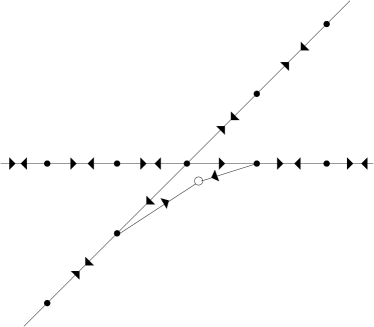
Figure 1: The representation ${\cal R}_{{1\over 3}}$.

Here we have arranged the circles representing the states according to their charges, with the horizontal axis corresponding to $J^{3}_{0}$, and the vertical axis to $L_{0}$. The horizontal array of circles represent the states of the form $(m-{1\over 3},-{1\over 3})$ with $m\in{\sf Z\!\!Z}$, where the quantum numbers of a state $(m,h)$ are given as

$$J^{3}_{0}(m,h) = m(m,h)$$ (5.25)

$$L_{0}(m,h) = h(m,h)\,.$$ (5.26)

On the other hand, the diagonal array of circles represents the states $(m-{1\over 3},m-{1\over 3})$, $m\in{\sf Z\!\!Z}$. The two arrays intersect at $(-{1\over 3},-{1\over 3})$, and the circle at this intersection corresponds to the state $(-{1\over 3},-{1\over 3})_{1}$. The arrows indicate the action of $J^{\pm}_{0}$ (for the horizontal line) and $J^{\pm}_{\mp 1}$ (for the diagonal line). Finally, the empty circle represents the state $(-{1\over 3},-{1\over 3})_{2}$ whose position in the charge lattice has been slightly shifted so that it does not lie on top of the other state with these charges. More specifically, we have the relations

$$J^{+}_{0}\left(-{1\over 3},-{1\over 3}\right) = \left({2\over 3},-{1\over 3}\right)\,,$$ (5.27)

$$J^{-}_{0}\left({2\over 3},-{1\over 3}\right) = J^{+}_{-1}\left(-{4\over 3},-{4\over 3}\right)\,,$$ (5.28)

and

$$J^{-}_{0}J^{+}_{0}\left(-{1\over 3},-{1\over 3}\right)_{1}={1\over 3}\left(-{1\over 3},-{1\over 3}\right)_{2}=J^{+}_{-1}J^{-}_{1}\left(-{1\over 3},-{1\over 3}\right)_{1}\,.$$ (5.29)

Furthermore we find that

$$L_{0}\left(-{1\over 3},-{1\over 3}\right)_{1} = -{1\over 3}\left(-{1\over 3},-{1\over 3}\right)_{1}+\left(-{1\over 3},-{1\over 3}\right)_{2}$$ (5.30)

$$L_{0}\left(-{1\over 3},-{1\over 3}\right)_{2} = -{1\over 3}\left(-{1\over 3},-{1\over 3}\right)_{2}\,.$$ (5.31)

Thus the representation ${\cal R}_{-{1\over 3}}$ is in fact a logarithmic representation. This does not contradict what we have found before since ${\cal R}_{-{1\over 3}}$ is not a highest weight representation. In fact, it was shown in [27] that with these relations one finds that

$$V_{0}({\cal N})\left(-{1\over 3},-{1\over 3}\right)_{1}=0\,,$$ (5.32)

where ${\cal N}$ is the null-vector in (5.5).

The representation ${\cal R}_{{1\over 3}}$ is not the only logarithmic representation that occurs in fusion products of the Kac-Wakimoto representations. In fact, the relevant representations also contain an extension of the vacuum representation ${\cal R}_{0}$

$$\left(E_{0}\otimes E_{0}\right)_{\mathrm{f}}={\cal R}_{0}\oplus E_{0}\,,$$ (5.33)

whose structure can be schematically described by figure 2.

Figure 2: The representation ${\cal R}_{0}$.

Here, as before, the different states have been arranged according to their $J^{3}_{0}$ and $L_{0}$ charge. The horizontal line represents states with charges $(m,0)$, $m\in{\sf Z\!\!Z}$, and the arrows correspond to the action of $J^{\pm}_{0}$. The state $(0,0)$ corresponds to $\omega$, and the empty circle represents the state $\Omega$ whose position in the charge lattice has been slightly shifted so that it does not lie on top of the state $\omega$. The arrows along the diagonal arrays correspond to the action of $J^{\pm}_{\pm 1}$ and $J^{\pm}_{\mp 1}$, respectively. More specifically, we have the relations

$$J^{-}_{-1}J^{+}_{1}\omega=\Omega=J^{+}_{-1}J^{-}_{1}\omega\,,$$ (5.34)

$$J^{-}_{0}J^{+}_{0}\omega=\gamma\Omega=J^{-}_{0}J^{+}_{0}\omega\,,$$ (5.35)

and

$$L_{0}\omega=\left(3+{3\over 2}\gamma\right)\Omega\,,$$ (5.36)

where $\gamma\neq 0,-2$ is a constant (that was not determined in [27]). Thus the two states $\omega$ and $\Omega$ form again the familiar Jordan block!

One can actually determine at least some of the remaining fusion rules explicitly; under some natural assumption (that is described in [27]) one then finds that the fusion rules close among the representations ${\cal H}_{0}$, $D^{\pm}_{j}$, $E_{0}$, ${\cal R}_{0}$ and ${\cal R}_{{1\over 3}}$, together with their images under $\pi_{s}$. More specifically, one finds

$$\left(D^{-}_{{1\over 3}}\otimes{\cal R}_{0}\right)_{\mathrm{f}} = {\cal R}_{{1\over 3}}$$ (5.37)

$$\left(D^{-}_{{1\over 3}}\otimes{\cal R}_{{1\over 3}}\right)_{\mathrm{f}} = 2\,\pi_{1}(E_{0})\oplus\pi_{1}({\cal R}_{0})$$ (5.38)

$$\left(E_{0}\otimes{\cal R}_{0}\right)_{\mathrm{f}} = 2\,E_{0}$$ (5.39)

$$\left(E_{0}\otimes{\cal R}_{{1\over 3}}\right)_{\mathrm{f}} = 2\,{\cal R}_{{1\over 3}}$$ (5.40)

$$\left({\cal R}_{0}\otimes{\cal R}_{0}\right)_{\mathrm{f}} = 2\,{\cal R}_{0}$$ (5.41)

$$\left({\cal R}_{0}\otimes{\cal R}_{{1\over 3}}\right)_{\mathrm{f}} = 2\,{\cal R}_{{1\over 3}}$$ (5.42)

$$\left({\cal R}_{{1\over 3}}\otimes{\cal R}_{{1\over 3}}\right)_{\mathrm{f}} = 2\,\pi_{1}({\cal R}_{0})\oplus 4\,\pi_{1}(E_{0})\,.$$ (5.43)

Together with (5.14) this then determines all fusion products.

6 Conclusions

In these lectures we have described how logarithmic conformal field theories can be understood from an algebraic (representation theoretic) point of view. We have explained how this point of view is related to the description of logarithmic conformal field theory in terms of amplitudes with logarithmic branch cuts. We have also shown that the algebraic approach is quite general and that it allows one to describe logarithmic representations that would be difficult to characterise otherwise. In particular, this is the case for logarithmic representations that are not obtained by the action of the chiral algebra from a highest weight state.

We have mainly considered the triplet theory at $c=-2$ which is the best understood (rational) logarithmic conformal field theory. We have analysed its fusion rules in detail, and we have described how to construct the corresponding local theory. Most of the logarithmic conformal field theories that have been studied so far are closely related to the $c=-2$ Virasoro model or an extension thereof.

In the last section we have shown that the $su(2)$ model at $k=-4/3$ is also a logarithmic conformal field theory. This result suggests that the same will presumably be the case for all other WZW models at fractional level. The logarithmic representations of these theories are presumably not highest weight representations, and their structure is therefore likely to be subtle. It would be very interesting to study these representations in more detail, and to get some better understanding of their general structure.

Given that already WZW models at fractional level appear to be logarithmic, it seems reasonable to speculate that most non-rational theories will actually be logarithmic. If one wants to obtain some more general understanding of non-rational theories, it will in particular be necessary to get to grips with logarithmic conformal field theories. It is hoped that the present notes will prove useful for that purpose.

Appendix A: The algebra structure of Zhu’s algebra

In this appendix we want to show that the product defined by (3.29) makes $A({\cal H}_{0})$ into an algebra. In order to exhibit the structure of this algebra it is useful to introduce a second set of modes by

$$V^{(N)}_{c}(\psi)=(-1)^{N}\oint{dw\over w}{1\over(w+1)}\left({w+1\over w}\right)^{N}V\left((w+1)^{L_{0}}\psi,w\right)\,.$$ (A.1)

These modes are characterised by the property that

$$\langle\bar{\phi}|\phi(-1)\;V^{(N)}_{c}(\psi)\;\chi\rangle = 0\qquad\hbox{for $N>0$,}$$ (A.2)

$$\langle\bar{\phi}|\phi(-1)\;V^{(0)}_{c}(\psi)\;\chi\rangle = \langle\bar{\phi}|\left(V_{0}(\psi)\phi\right)(-1)\;\chi\rangle\,.$$ (A.3)

It is obvious from (3.25) and (A.1) that

$$V^{(1)}(\psi)=V^{(1)}_{c}(\psi)\,,$$

and the analogue of (3.28) is

$$V^{(N+1)}_{c}(\psi)=-{1\over N+1}V^{(N)}_{c}(L_{-1}\psi)-{N+h_{\psi}\over N+1}V^{(N)}_{c}(\psi)\,.$$ (A.4)

The space $O({\cal H}_{0})$ is therefore also generated by the states

$$O({\cal H}_{0})=\hbox{span}\left\{V^{(1)}_{c}(\psi)\chi\,:\,\psi,\chi\in{\cal H}_{0}\right\}\,.$$

Let us introduce, following (3.30) and (A.3), the notation

$$V_{L}(\psi) \equiv V^{(0)}(\psi)$$

$$V_{R}(\psi) \equiv V^{(0)}_{c}(\psi)$$

$$N(\psi) = V^{(1)}(\psi)=V^{(1)}_{c}(\psi)\,.$$

We also denote by $N({\cal H}_{0})$ the vector space of operators that are spanned by $N(\psi)$ for $\psi\in{\cal H}_{0}$; then $O({\cal H}_{0})=N({\cal H}_{0}){\cal H}_{0}$. Finally it follows from the fact that the vacuum $\Omega$ is annihilated by all modes $V_{n}(\psi)$ with $n>-h_{\psi}$ together with $V_{-h_{\psi}}(\psi)\Omega=\psi$ that

$$V_{L}(\psi)\Omega=V_{R}(\psi)\Omega=\psi\,.$$ (A.5)

The equations (3.30) and (A.3) suggest that the modes $V_{L}(\psi)$ and $V_{R}(\chi)$ commute up to an operator in $N({\cal H}_{0})$. In order to prove this it is sufficient to consider the case where $\psi$ and $\chi$ are both eigenvectors of $L_{0}$ with eigenvalues $h_{\psi}$ and $h_{\chi}$, respectively. Then we have

$${}[V_{L}(\psi),V_{R}(\chi)] = \oint\oint_{|\zeta|>|w|}{d\zeta\over\zeta}(\zeta+1)^{h_{\psi}}{dw\over w}(w+1)^{h_{\chi}-1}V(\psi,\zeta)V(\chi,w)$$ (A.6)

$$\qquad-\oint\oint_{|w|>|\zeta|}{dw\over w}(w+1)^{h_{\chi}-1}{d\zeta\over\zeta}(\zeta+1)^{h_{\psi}}V(\chi,w)V(\psi,\zeta)$$

$$= \oint_{0}\left\{\oint_{w}{d\zeta\over\zeta}(\zeta+1)^{h_{\psi}}V(\psi,\zeta)V(\chi,w)\right\}{dw\over w}(w+1)^{h_{\chi}-1}$$

$$= \sum_{n}\oint_{0}\left\{\oint_{w}{d\zeta\over\zeta}(\zeta+1)^{h_{\psi}}V(V_{n}(\psi)\chi,w)(\zeta-w)^{-n-h_{\psi}}\right\}$$

$$\qquad\qquad{dw\over w}(w+1)^{h_{\chi}-1}$$

$$= \sum_{h_{\chi}\geq n\geq 0}\sum_{l=0}^{n+h_{\psi}-1}(-1)^{l}\,{h_{\psi}\choose l+1-n}$$

$$\qquad\qquad\oint_{0}{dw\over w(w+1)}\left({w+1\over w}\right)^{l+1}(w+1)^{h_{\chi}-n}V(V_{n}(\psi)\chi,w)$$

$$\in N({\cal H}_{0})\,.$$

Because of (A.4), every element in $N({\cal H}_{0})$ can be written as $V_{R}(\phi)$ for a suitable $\phi$, and (A.6) thus implies that $[V_{L}(\psi),N(\chi)]\in N({\cal H}_{0})$; hence $V_{L}(\psi)$ defines an endomorphism of ${\cal A}({\cal H}_{0})$.

For two endomorphisms, $\Phi_{1},\Phi_{2}$, of ${\cal H}_{0}$, which leave $O({\cal H}_{0})$ invariant (so that they induce endomorphisms of ${\cal A}({\cal H}_{0}))$, we shall write $\Phi_{1}\approx\Phi_{2}$ if they agree as endomorphisms of ${\cal A}({\cal H}_{0})$, i.e. if $(\Phi_{1}-\Phi_{2}){\cal H}_{0}\subset O({\cal H}_{0})$. Similarly we write $\phi\approx 0$ if $\phi\in O({\cal H}_{0})$.

In the same way in which the action of $V(\psi,z)$ is uniquely characterised by locality and its action on the vacuum (see [55]), we can now prove the following

Uniqueness Theorem for Zhu modes [50]: Suppose $\Phi$ is an endomorphism of ${\cal H}_{0}$ that leaves $O({\cal H}_{0})$ invariant and satisfies

$$\Phi\Omega = \psi$$

$${}[\Phi,V_{R}(\chi)] \in N({\cal H}_{0})\quad\hbox{for all $\chi\in{\cal H}_{0}$.}$$

Then $\Phi\approx V_{L}(\psi)$.

Proof: This follows from

$$\Phi\,\chi=\Phi\,V_{R}(\chi)\Omega\approx V_{R}(\chi)\,\Phi\,\Omega=V_{R}(\chi)\psi=V_{R}(\chi)\,V_{L}(\psi)\,\Omega\approx V_{L}(\psi)\chi\,,$$

where we have used that $V_{L}(\psi)\Omega=V_{R}(\psi)\Omega=\psi$.

It is then an immediate consequence that

$$V_{L}(V_{L}(\psi)\chi)\approx V_{L}(\psi)V_{L}(\chi)\,,$$ (A.7)

and a particular case of this (using again the fact that every element in $N({\cal H}_{0})$ can be written as $V_{L}(\phi)$ for some suitable $\phi$) is that

$$V_{L}(N(\psi)\chi)\approx N(\psi)V_{L}(\chi)\,.$$ (A.8)

In particular this implies that the product (3.29) $\phi\ast_{L}\psi$ is well-defined for both $\phi,\psi\in{\cal A}({\cal H}_{0})$. Furthermore, (A.7) shows that this product is associative, and thus ${\cal A}({\cal H}_{0})$ has the structure of an algebra.

We can also define a product by $\phi\ast_{R}\psi=V_{R}(\phi)\psi$. Since

$$\phi\ast_{L}\psi=V_{L}(\phi)\psi=V_{L}(\phi)V_{R}(\psi)\Omega\approx V_{R}(\psi)V_{L}(\phi)\Omega=V_{R}(\psi)\phi=\psi\ast_{R}\phi$$

this defines the reverse ring (or algebra) structure.

References

• [1] H. Saleur, Polymers and percolation in two dimensions and twisted $N=2$ supersymmetry, Nucl. Phys. B382, 486 (1992); hep-th/9111007.
• [2] M.A. Flohr, On modular invariant partition functions of conformal field theories with logarithmic operators, Int. J. Mod. Phys. A11, 4147 (1996); hep-th/9509166.
• [3] H.G. Kausch, Curiosities at $c=-2$, preprint DAMTP 95-52, hep-th/9510149.
• [4] G.M.T. Watts, A crossing probability for critical percolation in two dimensions, J. Phys. A29, L363 (1996); cond-mat/9603167.
• [5] M.R. Rahimi Tabar, S. Rouhani, The Alf’ven effect and conformal field theory, Nuovo Cimento 112B, 1079 (1997); hep-th/9507166.
• [6] M. Flohr, Two-dimensional turbulence: yet another conformal field theory solution, Nucl. Phys. B482, 567 (1996); hep-th/9606130.
• [7] M.R. Rahimi Tabar, S. Rouhani, A logarithmic conformal field theory solution for two dimensional magnetohydrodynamics in presence of the Alf’ven effect, Europhys. Lett. 37, 447 (1997); hep-th/9606143.
• [8] V. Gurarie, M. Flohr, C. Nayak, The Haldane-Rezayi quantum hall state and conformal field theory, Nucl. Phys. B498, 513 (1997); cond-math/9701212.
• [9] K. Ino, Modular invariants in the fractional quantum hall effect, Nucl. Phys. B532, 783 (1998); cond-mat/9804198.
• [10] S. Mathieu, P. Ruelle, Scaling fields in the two-dimensional abelian sandpile model, hep-th/0107150.
• [11] J.-S. Caux, I.I. Kogan, A.M. Tsvelik, Logarithmic operators and hidden continuous symmetry in critical disordered models, Nucl. Phys. B466, 444 (1996); hep-th/9511134.
• [12] J.-S. Caux, I.I. Kogan, A. Lewis and A.M. Tsvelik, Logarithmic operators and dynamical extension of the symmetry group in the bosonic $SU(2)_{0}$ and SUSY $SU(2)_{2}$ WZNW models, Nucl. Phys. B489, 469 (1997); hep-th/9606138.
• [13] Z. Maassarani, D. Serban, Non-unitary conformal field theory and logarithmic operators for disordered systems, Nucl. Phys. B489, 603 (1997); hep-th/9605062.
• [14] J.-S. Caux, N. Taniguchi, A.M. Tsvelik, Disordered Dirac fermions: multifractality termination and logarithmic conformal field theories, Nucl. Phys. B525, 671 (1998); cond-mat/9801055.
• [15] S. Guruswamy, A. LeClair, A.W.W. Ludwig, $gl(N|N)$ super-current algebras for disordered Dirac fermions in two dimensions, Nucl. Phys. B583, 475 (2000); cond-mat/9909143.
• [16] A.W.W. Ludwig, A free field representation of the $Osp(2|2)$ current algebra at level $k=-2$, and Dirac fermions in a random $SU(2)$ gauge potential, cond-mat/0012189.
• [17] M.R. Gaberdiel, H.G. Kausch, A rational logarithmic conformal field theory, Phys. Lett. B386, 131 (1996); hep-th/9606050.
• [18] M.R. Gaberdiel, H.G. Kausch, A local logarithmic conformal field theory, Nucl. Phys. B 538, 631 (1999); hep-th/9807091.
• [19] E. Verlinde, Fusion rules and modular transformations in 2D conformal field theory, Nucl. Phys. B300 [FS22], 360 (1988).
• [20] G. Moore, N. Seiberg, Polynomial equations for rational conformal field theories, Phys. Lett. B212, 451 (1988).
• [21] L. Rozansky, H. Saleur, Quantum field theory for the multi-variable Alexander-Conway polynomial, Nucl. Phys. B376, 461 (1992); hep-th/9203069.
• [22] V. Gurarie, Logarithmic operators in conformal field theory, Nucl. Phys. B410, 535 (1993); hep-th/9303160.
• [23] M.R. Gaberdiel, H.G. Kausch, Indecomposable fusion products, Nucl. Phys. B477, 293 (1996); hep-th/9604026.
• [24] A. Bilal, I.I. Kogan, On gravitational dressing of 2D field theories in chiral gauge, Nucl. Phys. B449, 569 (1995); hep-th/9503209.
• [25] A. Nichols, Logarithmic currents in the $SU(2)_{0}$ WZNW model, Phys. Lett. B516, 439 (2001); hep-th/0102156.
• [26] I.I. Kogan, A. Nichols, $SU(2)_{0}$ and $OSp(2|2)_{-2}$ WZNW models : two current algebras, one logarithmic CFT, hep-th/0107160.
• [27] M.R. Gaberdiel, Fusion rules and logarithmic representations of a WZW model at fractional level, hep-th/0105046, to appear in Nucl. Phys. B.
• [28] M. Flohr, Singular vectors in logarithmic conformal field theories, Nucl. Phys. B514, 523 (1998); hep-th/9707090.
• [29] M.A. Flohr, Bits and pieces in logarithmic conformal field theory, hep-th/0111228.
• [30] A. Shafiekhani, M.R. Rahimi Tabar, Logarithmic operators in conformal field theory and the ${\cal W}_{\infty}$-algebra, Int. J. Mod. Phys. A12, 3723 (1997); hep-th/9604007.
• [31] M.R. Rahimi Tabar, A. Aghamohammadi, M. Khorrami, The logarithmic conformal field theories, Nucl. Phys. B497, 555 (1997); hep-th/9610168.
• [32] M. Khorrami, A. Aghamohammadi, M.R. Rahimi Tabar, Logarithmic conformal field theories with continuous weights, Phys. Lett. B419, 179 (1998); hep-th/9711155.
• [33] M.A. Flohr, Operator product expansion in logarithmic conformal field theory, hep-th/0107242.
• [34] M.R. Rahimi Tabar, Lectures given at the school.
• [35] F. Rohsiepe, On reducible but indecomposable representations of the Virasoro algebra, hep-th/9611160.
• [36] I.I. Kogan, J.F. Wheater, Boundary logarithmic conformal field theory, Phys. Lett. B486, 353 (2000); hep-th/0003184.
• [37] Y. Ishimoto, Boundary states in boundary logarithmic CFT, hep-th/0103064.
• [38] S. Kawai, J.F. Wheater, Modular transformation and boundary states in logarithmic conformal field theory, Phys. Lett. B508, 203 (2001); hep-th/0103197.
• [39] Y. Ishimoto, Lectures given at the school.
• [40] S. Kawai, Lectures given at the school.
• [41] P. Ginsparg, Applied conformal field theory, in: Fields, strings and critical phenomena, eds. E. Brezin, J. Zinn-Justin, North-Holland, Amsterdam (1990).
• [42] Ph. Di Francesco, P. Mathieu, D. Sénéchal, Conformal field theory, Springer, New York, Berlin, Heidelberg (1996).
• [43] M.R. Gaberdiel, An introduction to conformal field theory, Rept. Prog. Phys. 63, 607 (2000); hep-th/9910156.
• [44] Y. Zhu, Vertex operator algebras, elliptic functions and modular forms, J. Amer. Math. Soc. 9, 237 (1996).
• [45] M.R. Gaberdiel, Fusion in conformal field theory as the tensor product of the symmetry algebra, Int. J. Mod. Phys. A9, 4619 (1994); hep-th/9307183.
• [46] W. Nahm, Quasi-rational fusion products, Int. J. Mod. Phys. B8, 3693 (1994); hep-th/9402039.
• [47] C. Dong, G. Mason, Vertex operator algebras and moonshine: A survey, Advanced Studies in Pure Mathematics 24, 101 (1996).
• [48] H.G. Kausch, Extended conformal algebras generated by a multiplet of primary fields, Phys. Lett. B259, 448 (1991).
• [49] E. Witten, Non-abelian bosonization in two dimensions, Commun. Math. Phys. 92, 455 (1984).
• [50] M.R. Gaberdiel, P. Goddard, Axiomatic Conformal Field Theory, Commun. Math. Phys. 209, 549 (2000); hep-th/9810019.
• [51] I.B. Frenkel, Y. Zhu, Vertex operator algebras associated to representations of affine and Virasoro algebras, Duke. Math. Journ. 66, 123 (1992).
• [52] B.L. Feigin, T. Nakanishi, H. Ooguri, The annihilating ideals of minimal models, Int. J. Mod. Phys. A7, 217 (1992).
• [53] W. Eholzer, A. Honecker, R. Hübel, How complete is the classification of ${\cal W}$-symmetries?, Phys. Lett. B308, 42 (1993).
• [54] W. Eholzer, M. Flohr, A. Honecker, R. Hübel, W. Nahm, R. Varnhagen, Representations of $W$-algebras with two generators and new rational models, Nucl. Phys. B383, 249 (1992).
• [55] P. Goddard, Meromorphic conformal field theory, in: Infinite dimensional Lie Algebras and Lie Groups, ed. V.G. Kac, page 556, World Scientific, Singapore, New Jersey, Hong Kong, (1989).
• [56] M.R. Gaberdiel, A. Neitzke, Rationality, quasirationality and finite W-algebras, DAMTP-2000-111, hep-th/0009235.
• [57] W. Wang, Rationality of Virasoro vertex operator algebras, Int. Math. Res. Not. 7, 197 (1993).
• [58] V.G. Kac, Infinite-dimensional Lie algebras, Cambridge (1990).
• [59] H.G. Kausch, Symplectic fermions, Nucl. Phys. B583, 513 (2000); hep-th/0003029.
• [60] M.R. Gaberdiel, Fusion of twisted representations, Int. Journ. Mod. Phys. A 12, 5183 (1997); hep-th/9607036.
• [61] P. Ginsparg, Curiositites at $c=1$, Nucl. Phys. B295, 153 (1988).
• [62] D. Gepner, E. Witten, String theory on group manifolds, Nucl. Phys. B278, 493 (1986).
• [63] M.A. Walton, Fusion rules in Wess-Zumino-Witten models, Nucl. Phys. B340, 777 (1990).
• [64] P. Furlan, A.Ch. Ganchev, V.B. Petkova, Quantum groups and fusion rules multiplicities, Nucl. Phys. B343, 205 (1990).
• [65] V.G. Kac, M. Wakimoto, Modular invariant representations of infinite dimensional Lie algebras and superalgebras, Proc. Natl. Acad. Sci. USA 85, 4956 (1988).
• [66] I.G. Koh, P. Sorba, Fusion rules and (sub)-modular invariant partition functions in non-unitary theories, Phys. Lett. B215, 723 (1988).
• [67] P. Mathieu, M.A. Walton, Fractional level Kac-Moody algebras and nonunitary coset conformal field theories, Prog. Theor. Phys. Suppl. 102, 229 (1990).
• [68] D. Bernard, G. Felder, Fock representations and BRST cohomology in $sl(2)$ current algebra, Commun. Math. Phys. 127, 145 (1990).
• [69] S. Panda, Fractional level current algebras and spectrum of $C<1$ minimal models coupled to gravity, Phys. Lett. B251, 61 (1990).
• [70] H. Awata, Y. Yamada, Fusion rules for the fractional level $\widehat{sl(2)}$ algebra, Mod. Phys. Lett. A7, 1185 (1992).
• [71] V.S. Dotsenko, Solving the $su(2)$ conformal field theory with the Wakimoto free field representation, Nucl. Phys. B358, 547 (1991).
• [72] B. Feigin, F. Malikov, Fusion algebra at a rational level and cohomology of nilpotent subalgebras of supersymmetric $sl(2)$, Lett. Math. Phys. 31, 315 (1994); hep-th/9310004.
• [73] O. Andreev, Operator algebra of the $SL(2)$ conformal field theories, Phys. Lett. B363, 166 (1995); hep-th/9504082.
• [74] C. Dong, H. Li, G. Mason, Vertex operator algebras associated to admissible representations of $\hat{sl}_{2}$, Commun. Math. Phys. 184, 65 (1997); q-alg/9509026.
• [75] J.L. Petersen, J. Rasmussen, M. Yu, Fusion, crossing and monodromy in conformal field theory based on $sl(2)$ current algebra with fractional level, Nucl. Phys. B481, 577 (1996); hep-th/9607129.
• [76] P. Furlan, A.Ch. Ganchev, V.B. Petkova, $A_{1}^{(1)}$ admissible representations – fusion transformations and local correlators, Nucl. Phys. B491, 635 (1997); hep-th/9608018.
• [77] A.Ch. Ganchev, V.B. Petkova, G.M.T. Watts, A note on decoupling conditions for generic level $\hat{sl}(3)_{k}$ and fusion rules, hep-th/9906139.
• [78] B. Feigin, F. Malikov, Modular functor and representation theory of $\hat{sl}_{2}$ at a rational level, Contemp. Math. 202, 357 (1997); q-alg/9511011.
• [79] A. Pressley, G.B. Segal, Loop groups, Oxford University Press, Oxford (1986).
• [80] M.R. Gaberdiel, WZW models of general simple groups, Nucl. Phys. B460, 181 (1996); hep-th/9508105.