Kontsevich-Witten Model From 2+1 Gravity: New Exact Combinatorial Solution

Abstract

In previous publications ( J. Geom.Phys.38 (2001) 81-139  and references therein ) the partition function for 2+1 gravity was constructed for the fixed genus Riemann surface.With help of this function the dynamical transition from pseudo-Anosov to periodic (Seifert-fibered) regime was studied. In this paper the periodic regime is studied in some detail in order to recover major results of Kontsevich (Comm.Math.Phys. 147 (1992) 1-23 ) inspired by earlier work of Witten on topological two dimensional quantum gravity.To achieve this goal some results from enumerative combinatorics have been used. The logical developments are extensively illustrated using geometrically convincing figures. This feature is helpful for development of some non traditional applications (mentioned through the entire text) of obtained results to fields other than theoretical particle physics.

MCS:83C45

Subj.Class.:Quantum gravity

Keywords : Surface automorphisms; dynamical systems; gravity; Grassmannians; Schubert calculus; enumerative combinatorics.

1 Introduction

1.1 Motivation

It may not be exaggeration to say that dynamics of 2+1 gravity is just an interpretation of Nielsen -Thurston theory of surface homeomorphisms in terms of concepts known in physics [1-4]. Apparently, the reverse task  of enriching mathematics with concepts known from physics had been accomplished by Witten [5]. His physical intuition had revolutionized  combinatorial methods of algebraic geometry related to intersection theory  on moduli space of curves [6-8]. In his famous paper [9] Kontsevich had provided needed mathematical justification to Witten’s work. Since in both papers the initial object of study is 2 dimensional quantum gravity it is only natural to expect that the results of Witten and Kontsevich can be reobtained from more general 2+1 gravity model. The purpose of this paper is to demonstrate that this is indeed possible.

It should be noted that the results of Witten and Kontsevich (W-K) rely heavily on the fact (proven by Kontsevich [9]) that the partition function of 2d gravity happens to be $\ \tau$ function of the Korteweg-de Vries (KdV) hierarchy which is just a special case of  more general Kadomtsev-Petviashvili (KP) hierarchy of nonlinear exactly integrable  partial differential equations. Attempts to connect string theory with exactly integrable systems had been made earlier. Good summary of earlier efforts can be found in Ref.[10]. Recently, KP equations had been discussed in relation to dynamics of 2+1 gravity [11]. The content of Ref.[11] apparently has no connections with results of W-K. This does not exclude the possibility that such connection might exist and requires further study. In the present work we establish such connection (reduction) by reobtaining W-K results from formalism developed earlier for 2+1 gravity [1-4]. This formalism is based on some properties of Riemann surfaces. From algebraic geometry it is known that every Riemann surface $\mathcal{S}$ can be described in terms of the corresponding  complex algebraic curve $\mathcal{C}$ [12] so that one can use interchangeably algebro-geometric and complex analytic language to discuss the same object, the Riemann surface. This,unfortunately, is not an easy task as was noticed by Looijenga [7]. The existing difference in terminology is especially apparent when one is interested in the issue of compactification of the moduli space of Riemann surfaces (e.g. see Eq.(1.1) and related discussion)

Moduli spaces $\mathcal{M}_{g}$ are connected with Teichmüller spaces $\mathcal{T}_{g}$ of Riemann surfaces of genus $g\geq 2$ in such a way that $\mathcal{M}_{g}=$ $\mathcal{T}_{g}/\mathcal{\Gamma}$ with $\Gamma$ being the mapping class group of $\mathcal{S}$. Both $\mathcal{M}_{g}$ and ${}\mathcal{T}_{g}$ have been discussed extensively in our earlier published papers on 2+1 gravity [1-4]. The concept of moduli had been initially proposed by Riemann  who stated that isomorphism classes of closed Riemann surfaces of genus $g\geq 2$ are parametrized by 3g-3 complex parameters (or by 6g-6 real parameters). The space of allowed values of these parameters is effectively the moduli space $\mathcal{M}_{g}$ . More accurately, such moduli space is called coarse moduli space. It is complex analytic space of dimension 3g-3 but not a complex manifold. Presence of singularities (to be discussed below) prevents this manifold from becoming a complex manifold [6,13]. One way of describing both $\mathcal{M}_{g}$ and $\mathcal{T}_{g}$ is through introduction of marking of $\mathcal{S}$ (accordingly of $\mathcal{C}$ ). Marking of $\mathcal{S}$ can be made by introducing some $n$ boundary components such that each of them is conformally equivalent to a punctured disk [14]. Accordingly, for algebraic curves we select $n$ distinguished (smooth) points on the curve. Smooth means that the points are not located at the possible singularities of  $\mathcal{C}$. According to Deligne and Mumford [15] such singularities are regular double points which, in the case of  traditional visualization of  Riemann surfaces as  closed surfaces with $g$ holes, are associated with formation of nodes as depicted in Fig.1.

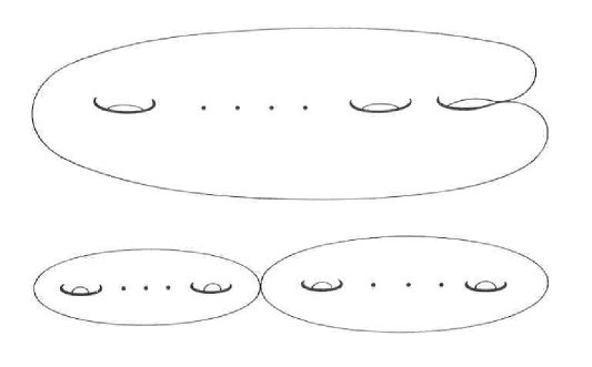
Figure 1: Various types of degeneration of the Riemann surfaces

The compactification $\mathcal{\bar{M}}_{g,n}$  of moduli space is achieved by inclusion into $\mathcal{M}_{g,n}$ domains in parameter space associated with Riemann surfaces with nodes. In the language of algebraic geometry  complex curves associated with such surfaces are called stable.  Marked curves possess only finitely many authomorphisms. It is known [6] that no stable curve can have more than 3g-3 nodes. This fact may be easily understood if we recall that each Riemann surface admits pants decomposition [2] so that 3g-3 nodes can be associated with degenerate geodesics whose lengths are squeezed to zero. For Riemann surface $\mathcal{S}$ instead of (or in addition to) marked points one can think about families of closed curves ( lamination sets [4]) and their intersections. By  properly defining intersection number(s) one can measure the nontriviality of such sets [6]. In algebraic geometry such numbers are associated with cohomology classes known also as $\mathit{tautological}$ classes $\psi_{i}$ in $H^{2}(\mathcal{\bar{M}}_{g,n},\mathbf{Q})$. These numbers should  not be confused with geometrical intersection numbers introduced by Thurston [16,17]. Roughly speaking such number $i$ measures the number of intersections between a selected simple nontrivial closed curve $\alpha$ on $\mathcal{S}$ and measured foliation $\mathcal{F}$: $i=i(\mathcal{F},\alpha)$.This observation allows one to introduce equivalence relations between measured foliations. In particular, foliations $\mathcal{F}_{1}$ and $\mathcal{F}_{2}$ are projectively equivalent if there is number $\lambda\in\mathbf{R}_{+}$ such that  $i$($\mathcal{F}_{1}$,$\alpha)=\lambda i(\mathcal{F}_{2},\alpha).$ Following Thurston [17]and others [18] , we define the space of projective laminations $\mathcal{PL}$($\mathcal{S}$)  as space of equivalence classes of measured foliations. Such defined space forms a boundary of the Teichmüller space $\mathcal{T}_{g,n}.$ The compactification of the Teichmüller space $\mathcal{\bar{T}}$($\mathcal{S}$) is defined now as

$$\mathcal{\bar{T}}(\mathcal{S})=\mathcal{T}(\mathcal{S})\cup\mathcal{PL}(\mathcal{S}).$$ (1.1)

The set $\mathcal{\bar{T}}(\mathcal{S})$ is closed ball of real dimension $6g-6+2n$ whose boundary is identified with $\mathcal{PL}$($\mathcal{S}$). Since the moduli space is the quotient of $\mathcal{T(S)}$ by the mapping class group $\Gamma$ , is clear that such defined compactification of the Teichmüller space leads accordingly to the compactification of the moduli space. Such compactificatioon is apparently different from that of Deligne-Mumford. The difference has some physical meaning. Indeed, in the traditional, algebro-geometric case, no dynamics is involved while in the Thurston’s case the dynamics (that is ”time evolution” ) is associated with dynamically formed 3-manifolds, e.g. see chapters 8 and 9 of Thurston’s lecture notes [16]. These dynamical features are explained in physical terms and illustrated in our recently published paper on statistical mechanics of 2+1 gravity [4] .

Since in 2 dimensional quantum gravity there is no time evolution, naturally, there is no dynamical observables and theory is essentially topological. Witten [5] had suggested to study the topological averages of the type

$$<\tau_{k_{1}}\cdot\cdot\cdot\tau_{k_{n}}>_{g}\equiv\int\nolimits_{\mathcal{\bar{M}}_{g,n}}\psi_{1}^{k_{1}}\cdot\cdot\cdot\psi_{n}^{k_{n}}$$ (1.2)

provided that $3g-3+n=\sum\nolimits_{i=1}^{n}k_{i}$ . To understand the meaning of such an average it is  instructive to consider the first nontrivial example: $g=1,n=1$. In this case we obtain,

$$<\tau_{1}>_{1}=\int\nolimits_{\mathcal{\bar{M}}_{1,1}}\psi.$$ (1.3)

Witten had demonstrated that $<\tau_{1}>_{1}=\frac{1}{24}$ . This result had been actually obtained earlier by Wolpert [19] who noticed that

$$<\tau_{1}>_{1}\dot{=}\frac{1}{2\pi^{2}}\int\nolimits_{\mathcal{\bar{M}}_{1,1}}\omega_{w-p}$$ (1.4)

where $\omega_{w-p}$ is familiar Weil-Petersson Kähler (1,1) form which plays very important role in both the theory of Teichmüller spaces [20] and in string theory [21]. The dot above the equality sign has the following meaning. The integral $\int\nolimits_{\mathcal{\bar{M}}_{1,1}}\omega_{w-p}$ had been independently calculated by Wolpert [22] and Penner [23] and is known to be equal to $\dfrac{\pi^{2}}{6}$ so that the right hand side of Eq.(1.4) is equal to $\frac{1}{12}.$ The same result was obtained by Witten [5] who argues that it should be additionally divided by 2 because ”the generic elliptic curve has two symmetries”.  Thus, evidently, computation of ”tautological averages”, Eq.(1.2), is effectively equivalent (up to numerical prefactors) to calculation of  the Weil-Petersson volumes of $\mathcal{\bar{M}}_{g,n}$. Zograf [24] had calculated such volumes for $n\geq 3$ punctured spheres. Based on these results, Matone [25] had developed and solved non pertubatively 2d Liouvillian gravity. Some of his results had been used and extended in the work by Kaufman, Manin and Zagier [26]. These results had been further streamlined in recently published monograph by Manin [27].

1.2 From Chern classes to Grassmannians

To make an additional connection with physics, we would like to reanalyze just obtained results from the point of view of differential geometry of complex manifolds [21,28]. In this regard, a closed integral (1,1) form $\omega$  on  a complex manifold $M$ determines the equivalence class of a line bundle $\lambda.$ Recall  [21] that a line bundle $\lambda$ on manifold M is an assignment of one dimensional  complex vector space $\lambda_{z}$ to each point $z\in M$ . Sections of $\lambda_{z}$ are some functions $f_{\alpha}$ ($z\in\mathcal{B}_{\alpha})$ assigning an element of $\lambda_{z}$ to each point $z$. Vector spaces at different points should fit together and this leads naturally to the fiber bundle constructions made of transition functions $\phi_{\alpha_{\beta}}$ between different coordinate charts $\mathcal{B}_{\alpha}$. A metric on $\lambda_{z}$  is a set of positive functions $g_{\alpha}$ such that $g_{\alpha}=\left|\phi_{\alpha_{\beta}}\right|^{2}g_{\beta}$. The covariant derivative is defined now as

$$\nabla_{j}f_{\alpha}=\{\frac{\partial}{\partial z_{j}}+\frac{\partial}{\partial z_{j}}\ln g_{\alpha}\}f_{\alpha}.$$ (1.5)

The bundle $\lambda$ is holomorphic if in addition

$$\bar{\nabla}_{j}f_{\alpha}=\frac{\partial}{\partial\bar{z}_{j}}f_{\alpha}\text{ .}$$ (1.6)

With help of such defined covariant derivative the curvature tensor $F$ of $\lambda$ is obtained in a standard way [28] with the result:

$$F=\frac{\partial^{2}}{\partial z\partial\bar{z}}\ln g_{\alpha}.$$ (1.7)

Finally, it can be shown [21,28], that

$$\omega=\frac{i}{2\pi}Fdz\wedge d\bar{z}$$ (1.8)

and that, actually, such defined (1,1) form coincides with the first Chern class form $c_{1}(\lambda)$. In our case $M=$ $\mathcal{\bar{M}}_{g,n}$ and the line bundle is actually a cotangent bundle $T^{\ast}(\mathcal{\bar{M}}_{g,n})$ made of quadratic differentials [Wolpert, positive] .Wolpert [29,30]  had demonstrated that

$$\frac{1}{\pi^{2}}\omega_{w-p}=\frac{i}{2\pi}F=c_{1}(\lambda).$$ (1.9)

Substituting this result into Eq.(1.4) we obtain,

$$<\tau_{1}>_{1}=\int\nolimits_{\mathcal{\bar{M}}_{1,1}}c_{1p}(\lambda),$$ (1.10)

where $c_{1p}(\lambda)$=$c_{1}(\lambda)/2$ . In  such notations this result coincides with Eq.(1.7) of Witten’s paper [5] (for $d=1$). The reason of introducing the factor of 1/2 can be explained as follows. According to Wells, Ref.[28], Ch-r 6, the traditional construction of Hodge line bundles for manifolds requires that

$$\int\omega=\operatorname{integer}=c.$$ (1.11)

Moreover, if $c$ is an integer, it is actually equal to the Euler characteristic of the manifold. In our case, $\mathcal{\bar{M}}_{1,1}$ is an orbifold and for the orbifolds the Euler number can be rational number according to Thurston [16]. Wells explains how to construct the Hodge bundle for any Kählerian manifold/orbifold. To this purpose, if the constant $c$ in Eq.(1.11) is not an integer, it is sufficient to rescale the form $\omega:\Omega=c^{-1}\omega$ , so that the rescaled form is the Hodge form. Since the moduli space $\mathcal{\bar{M}}_{g,n}$ is an orbifold, Eq.(1.10) is acceptable and, hence, with such remarks, coincides with Eq.(1.7) of Witten’s paper (for $d=1$), Ref.[5].

Obtained results possess additional  very important physical information allowing us to make direct  and simple connections with Grassmannians and, hence, with exactly integrable systems, using arguments different from that of Witten [5] and Kontsevich [9].

Let $G^{\mathbf{C}}(d,n)$ be complex Grassmann manifold. It  is known that

$$G^{\mathbf{C}}(d,n)=\frac{U(d+n)}{U(d)U(n)}.$$ (1.12)

where $U(n)$ belongs to the unitary  Lie group of $n\times n$ matrices. Following Ref.[31,32] consider now the classifying space $BU(n)$ defined by

$$BU(d)=\lim_{n\rightarrow\infty}\frac{U(d+n)}{U(d)U(n)}.$$ (1.13)

The name classifying comes from the following observation. Suppose there is a map $f$ from a base space $M$ to $BU(d)$, i.e. $f$: $M\rightarrow BU(d)$. Construction of such a map for the case of orbifolds has been developed by Baily [33] and, in particular, for $\mathcal{\bar{M}}_{g,n}$ by Wolpert [29]. The $n$-vector complex bundle $\lambda$ over the base space $M$ can be expressed as a pullback of the standard vector bundle $\xi$ over $BU(d)$ . That is $\lambda=f^{\ast}(\xi).$ The i-th Chern class $c_{i}^{\ast\text{ }}$ of the vector bundle $\lambda$ can then be calculated simply by the pullback $f^{\ast}(c_{i})$ $\in H^{2i}(M,R)$ of the element $c_{i}$ in the 2i-th cohomology group of $BU(d).$ $G^{\mathbf{C}}(d,n)$ can be embedded in the complex projective space. This can be achieved for any $n$ and the limiting case $n\rightarrow\infty$ is known as Sato Grassmannian in the theory of KP equations [34]. We would like now to describe such an embedding in some detail.

Recall that the complex projective space Pⁿ is defined as P${}^{n}:=(\mathbf{C}^{n+1}-\{\mathbf{0}\})/\sim$ with equivalence relation $\sim$ defined as follows. If a point $P\in$Pⁿ is given by an $n+1$ tuple ($z(0),...,z(n))$, then another $(n+1)$ tuple $(z\prime(0),...,z\prime(n))$ defines the same point  $P\in$Pⁿ if there is a  nonzero number $c$ such that $z(i)=cz\prime(i),$ $\forall i$ , $i=0-n.$The system of standard coordinates ($U_{i}$ ,$\varphi_{i})$ enables us to define a manifold structure on Pⁿ :

$$U_{i}:=\{(z(0),...,z(n))\mid z(i)\neq 0\},i=1-n$$

and

$$\varphi_{i}:U_{i}\rightarrow\mathbf{C}^{n}:=\text{ (}\frac{z(0)}{z(i)},...,\frac{z(i-1)}{z(i)},\frac{z(i+1)}{z(i)},...,\frac{z(n)}{z(i)}).$$ (1.14)

With help of such map $U_{i\text{ }}$ can be identified with the affine space Cⁿ and the space Pⁿ can be made from different coordinate patches $U_{i}$ with help of transition  functions $\phi_{\alpha_{\beta}}$ as discussed before. A linear space $\mathcal{L}$ in Pⁿ is defined as the set of points $P$=$(z(0),...,z(n))$ of Pⁿ whose coordinates satisfy a system of linear equations

$$\sum\nolimits_{j=0}^{n}b_{aj}z(j)=0$$ (1.15)

$\alpha=1,...,(n-d).$ The space $\mathcal{L}$ is $d$-dimensional if $(n-d)\times(n+1)$ matrix of coefficients [$b_{aj}]$ has a nonzero $(n-d)\times(n-d)$ minor. In this case there are $d+1$ points $P_{i}=$ ($z_{i}(0),...,z_{i}(n))$ in $\mathcal{L}$ ($i=0-d)$ which span $\mathcal{L}$ . Naturally, $\mathcal{L}$ is a line if $d=1$, a plane if $d=2$ and a hyperplane if $d>2$. We shall call these planes as $d$-planes following [35] . $d$-planes in Pⁿ can be represented by the points in the projective space P^N whose dimension $N$ is given by

$$N=\frac{\left(n+1\right)!}{\left(d+1\right)!(n-d)!}-1.$$ (1.16)

To this purpose, let us fix a $d$-plane in Pⁿ and pick $d+1$ points $P_{i}=$($z_{i}(0),...,z_{i}(n))$ which span $\mathcal{L}$. Using these points let us form $(d+1)\times(n+1)$ matrix [$p_{i}(j)]$ with $0\leq i\leq d$ and 0$\leq j\leq n.$ Let $j_{0},...,j_{d}$ be a sequence of integers with 0$\leq$ $j_{\beta}$ $\leq n$ and let $p(j_{0},...,j_{d})$ denote the determinant of $(d+1)\times(d+1)$ matrix $[p_{i}(j_{\beta})]$ with $i$,$\beta=0,...,d.$ There will be $N$+1 determinants of such type and at least one of them is nonzero by requirements of linear algebra. Hence, in view of Eq.(1.14), we conclude that we can use these determinants to determine a point in the complex projective space P${}^{N}.$ The coordinates of this point are called Plücker coordinates of $\mathcal{L}$ in P^N and such  an embedding of the complex Grassmannian manifold (of $d$-planes in Pⁿ space) into complex projective space P^N is called Plücker embedding. Not every point in P^N arises from $d$-plane in P${}^{n}.$ Plücker coordinates $p$($j_{0},...,j_{d})$ obey the following set of  (Plücker) equations

$$\sum\nolimits_{j=0}^{d+1}(-1)^{j}p(j_{0},...,j_{d-1}k_{j})p(k_{0},...,\check{k}_{j},...,k_{d+1})=0.$$ (1.17)

Here $j_{0},...,j_{d-1}$ and $k_{0},.,k_{d+1}$are sequences of  integers with 0$\leq j_{\beta}$ , $k_{\xi}\leq n$ with $\check{k}_{j}$ meaning that the integer $k_{j}$ has been removed from the sequence.

As it is shown by Miwa et al [34] Plücker coordinates represent  the location of tau function of the KP hierarchy inside the Grassmannian while Plücker equations are in one to one correspondence with the Hirota bilinear equations. Hence, the connection between the averages given by Eq.(1.2) and KP (or, more exactly, KdV) hierarchy naturally follows. The determinants, which are points in P${}^{N},$ have probabilistic meaning which is discussed below. To this purpose we have to introduce some additional concepts.

1.3 From Grassmannians to Schubert varieties

Consider a sequence of subspaces (cellular decomposition), i.e. $A_{0}\subset A_{1}\subset...\subset A_{d}$ of a fixed space, e.g. P${}^{n},$ each properly contained in the next, whose dimensions dim $A_{i}=a_{i}$ , provided that $0\leq a_{0}<a_{1}<...<a_{d}\leq n$ . Such construction is called flag. Let now $\Omega(A_{0},...,A_{d})$ be the subset $\mathcal{L}$ of $G^{\mathbf{C}}(d,n)$ consisting of all $d$-planes satisfying $\dim$ $(\mathcal{L\cap}A_{i})\geq i$ for $i$=$0,...,d.$ Thus, if $\dim$ $A_{i}=i$ $\forall i$ , then $\Omega(A_{0},...,A_{d})$ is made of a single $d$-plane, while if $\dim A_{i}=n-d+i$ $\forall i$ , then $\Omega(A_{0},...,A_{d})=G^{\mathbf{C}}(d,n).$

Definition 1.1. $\Omega(A_{0},...,A_{d})$ is called Schubert variety corresponding to the flag $A_{0}\subset A_{1}\subset...\subset A_{d}$ . $\Omega(A_{0},...,A_{d})$ defines a homology (actually, cellular homology [32] ) class in the homology ring $H_{\ast}$($G^{\mathbf{C}}(d,n);\mathbf{Z}).$

Definition 1.2.Homology class in $H_{\ast}$($G^{\mathbf{C}}(d,n);\mathbf{Z})$ is called Schubert cycle.Because the homology class depends only on the integers $a_{i}=$dim$A_{i}$ , it is appropriate to write $\Omega(A_{0},...,A_{d})=\Omega(a_{0},...a_{d})$ where 0$\leq a_{0}<a_{1}<...<a_{d}\leq n.$

It can be shown [12] that the product of any two Schubert cycles can be uniquely expressed as a linear combination of other Schubert cycles.This observation is central for development of Schubert calculus [12,35,36].

Remark 1.3. Gepner [37]  had demonstrated that  all  results of rational conformal field theories can be  actually obtained from physically reformulated Schubert calculus. Additional  physical refinements of these ideas can be found in the work by Witten [33].

$H_{\ast}$($G^{\mathbf{C}}(d,n);\mathbf{Z})$ is generated by the special Schubert cycles given by

$$\sigma(i)=\Omega(i,n-d+1,...,n)$$ (1.18)

for $i=0,1,...,n-d$. These results allow to prove [12,35,36] the following theorem of central importance for the whole development presented in the rest of this paper.

Theorem 1.4. For all sequences of integers 0 $\leq a_{0}<a_{1}<...<a_{d}\leq n$ (which we denote as a̱ ) the following determinantal (Giambelli’s-like) formula holds in the homology ring $H_{\ast}$($G^{\mathbf{C}}(d,n);\mathbf{Z}):$

$$\Omega(\text{\@text@baccent{a}})=\left|\sigma(a_{i}+j-i)\right|\text{ , 0}\leq i,j\leq n-d$$ (1.19)

with $\left|\sigma(a_{i}+j-i)\right|$ being a determinant made of special cycles.

Remark 1.5. The name Giambelli comes from the fact that structurally the same expression exist for the Schur polynomials S${}_{\text{\@text@baccent{a}}}$ which was discovered by Giambelli [39-42]. The Schur polynomials are characters of the general linear group on symmetrized complex linear vector space $E^{\text{\@text@baccent{a}}}$ [39-42]. In the light of results presented earlier we can associate the determinant $p$($j_{0},...,j_{d})$ with that for special Schubert cycles, Eq.(1.19), so that the Schur polynomials are tau functions of KP hierarchy. The formal correspondence between the Schur polynomials and Eq.(1.19) is not coincidental. It can be proven [42] that, actually, there is an isomorphism $\Theta$ between S${}_{\text{\@text@baccent{a}}}$ and $\Omega($a̱$)$.

Remark 1.6. The topological meaning of Eq.(1.19) had been clarified by Porteous [43] and also by Horrocks [44] and, later, by Carrel [45]. All these results can be actually deduced directly from much earlier fundamental papers by Chern [46] and Ehresmann [47].

We would like to describe briefly these results since they are essential for correct physical understanding of the meaning of intersection numbers. To this purpose let us observe that for $k$-cycle $A$ and $n-k$ cycle $B$ on an $n$-dimensional manifold $M$ the Poincare’ duals of these cycles are closed $n-k$ and $k$ differential forms $\varphi$ and $\psi$ respectively so that the intersection number ^#($A\cdot B)$ of these cycles in homology is equal to the wedge product of these two forms in cohomology [12], i.e.

$${}^{\#}(A\cdot B)=\int\limits_{M}\varphi\wedge\psi.$$ (1.20)

This definition can be extended to describe the intersection of subvarieties $V$ and $W$ of a complex manifold $M$ and it is possible to prove that Schubert calculus is just a special case of such more general algebra known in the literature as Chow algebra [8] (also as Chow ring [41]). Next, we need a notion of a divisor.

If the manifold $M$ can be decomposed as

$$M=V_{1}\cup\cdot\cdot\cdot\cup V_{m}$$ (1.21)

then one introduces

Definition 1.7.Divisor $D$ on $M$ is locally finite formal linear combination

$$D=\sum a_{i}V_{i}$$ (1.22)

of irreducible analytic hypersurfaces $V_{i}$ of $M$.

Definitions of ”local finitness” and ”irreducibility” are given in Ref.[12] on page 130.The constants $a_{i\text{ }}$ are normally some integers. For $G^{\mathbf{C}}(d,n)$ Schubert cycles provide the desired decomposition of the Grassmannian [12]. The following theorem is of central importance [12].

Theorem 1.8.The Chern class $c_{1}(\lambda),$ given by Eq.(1.9), of the line bundle $\lambda$ represents the Poincare’ dual of the fundamental homology cycle carried by the divisor D, i.e.

$$\frac{i}{2\pi}\int\limits_{M}F\wedge\psi=\sum a_{i}\int\limits_{V_{i}}\psi$$ (1.23)

for every real closed $2n-2$ form $\psi.$

Consider now some implications of this theorem. First, in the case if $M$ is compact Riemann surface, a divisor on $M$ is just a finite sum

$$D=\sum n_{i}p_{i}$$ (1.24)

of points $p_{i}\in M$  with multiplicities $n_{i}$. Combining Eqs.(1.23) and (1.24) produces the Poincare’-Hopf index theorem

$$\frac{i}{2\pi}\int\limits_{M}F=\sum\limits_{i}n_{i}=\chi(M).$$ (1.25)

This theorem played central role in our earlier works of 2+1 gravity [1,2].This observation clarifies both the meaning of numbers $n_{i}$ and points $p_{i}$ : for vector (or line) fields these points are associated with singularities of the field. These singularities had been interpreted as masses.

Remark 1.9. Generalization of this result to higher dimensions had been developed by Chern and Weil (CW). The up to date exposition and generalization of their results can be found in Ref.[48] and, in principle, provides an opportunity to describe 3+1 gravity in a way similar to that developed for 2+1 dimensional case. Such approach to gravity is very close in spirit to that originally suggested by Regge [49].

We need this observation in the present context as well for the following reasons. By definition, a subset $V$ of an open set $U\in\mathbf{C}^{n}$ is an analytic variety if for any $p\in U$ there exists a neighborhood $U^{{}^{\prime}}$ of $p$ in $U$ such that $V\cap U^{\prime}$ is common zero locus of a finite collection of holomorphic functions $\{f_{i}\}$ on $U^{{}^{\prime}}.$ In particular, $V$ is called an analytic hypersurface if locally $V$ is zero locus of a single nonzero holomorphic function $f$, i.e.$V=\{f(z)=0\}$ in the neighborhood of $0\in V$. Accordingly, for decomposition, Eq.(1.21), $V_{i}=\{f_{i}(z)=0\}$ with $V_{i}$ irreducible at $0$ . All these facts lead to the following

Definition 1.10. An algebraic variety $V\subset\mathbf{P}^{n}$ is the image in Pⁿ of  zero locus of a collection of homogenous polynomials defined in Cⁿ⁺¹, i.e. $V$=( $\mathcal{F}_{i}(z_{0},...,z_{n})=0).$

For the line bundle $\lambda$ on $M$ it is possible to associate sections with $\mathcal{F}_{i}$ if $M$ can be embedded into P${}^{n}($and, in our case, it can be embedded since we had mentioned already that $\lambda=f^{\ast}(\xi)$ with $\xi\in BU(n)$). Suppose now that for some point $z^{\ast}\in M$ of $n$-dimensional complex manifold $m$ sections are linearly dependent. Then, according to CW theory [48,50], this fact can be written as

$$f_{\alpha_{1}}\wedge\cdot\cdot\cdot\wedge f_{\alpha_{m}}=0.$$ (1.26)

This equation is multidimensional analogue of the Poincare’ condition (e.g. read Remark 4.2. of Ref [2]) for the singularities of the line/vector fields on surfaces. The degeneracy set is set of all points $z_{i}^{\ast}$ for which condition given by Eq.(1.26) holds. In the most general case it is $m-1$ dimensional submanifold D̂ of $M$. Consider now a cycle $\alpha$ on $M$ of dimension $r$ lesser than that of D̂. Let such a cycle meet D̂ transversely at the point $z_{i}^{\ast}\in$D̂ then, $f$($\alpha)$ will meet some Schubert cycle $\Omega($a̱$)$ also transversely at the point $f(z_{i}^{\ast})$ of the Grassmannian so that the intersection number of $f$($\alpha)$ with $\Omega($a̱$)$ at $f(z_{i}^{\ast})$  will be the same as that for $\alpha$ meeting D̂ on $M$. Taking into account Eq.s(1.20) and (1.23) and also Theorem 1.8., we conclude that $c_{r}(\lambda)(\alpha)=$ ${}^{\#}(\alpha,$D̂$).$ With little additional work it can be shown [12] that

$$\Omega(\alpha)=\left|c_{\alpha_{i}+j-i}(\lambda)\right|\text{ , }0\leq i,j\leq n-d,$$ (1.27)

to be compared with Eq.(1.19). This result was obtained by Porteous [43] and is known in the literature as Porteous formula [12,41].

1.4 From Schubert varieties to directed random walks

Porteous formula can be seen as a special case of much more comprehensive result of Weil (and developed by Chern ) known as Weil homomorphism. In view of this homomorphism, the result given by Eq.(1.27) can be reinterpreted as Schur polynomial (e.g. read discussion following Eq.(1.19)) and, hence, as $\tau$ function of KP hierarchy. Schur polynomials S_λ originate from the known [40] identity for indeterminates $\{x_{i}\}$

$$\left(x_{1}+\cdot\cdot\cdot+x_{m}\right)^{n}=\sum\limits_{\lambda\vdash n}f^{\lambda}\text{S}_{\lambda}(x_{1},...,x_{m}),$$ (1.28)

where use of the notation $\lambda\vdash n$ is meant to say that $\lambda$ is partition of $n$. Partitions are best represented by the Young tableaux. Accordingly, the factor $f^{\lambda}$ denotes a number of standard tableaux of a given shape $\lambda$ .

Eq.(1.28) can be rewritten in a slightly different form as follows

$$\left(x_{1}+\cdot\cdot\cdot+x_{n}\right)^{M}=\sum\limits_{\left(m_{1},...,m_{n}\right)}\frac{M!}{m_{1}!m_{2}!...m_{n}!}x_{1}^{m_{1}}\cdot\cdot\cdot x_{n}^{m_{n}}$$ (1.29)

provided that $M=m_{1}+\cdot\cdot\cdot+m_{n}.$ This observation allows us to write Schur polynomial S_λ in the form

$$\text{S}_{\lambda}(x_{1},...,x_{n})=\sum\limits_{m=\left(m_{1},...,m_{n}\right)}K_{\lambda,m}x_{1}^{m_{1}}\cdot\cdot\cdot x_{n}^{m_{n}}$$ (1.30)

with $K_{\lambda,m}$ being some coefficients (Kostka numbers) [42].

Eq.(1.30) can be given probabilistic meaning in terms of the directed random walks. Indeed, following Ref.[42,51], consider planar lattice. On this lattice consider a directed path P from (a,1) to (b,N). The information about this path can be encoded into multiset $Hor_{y}$(P) of $y-$coordinates of the horizontal steps of P. Define

$$\text{w}(\text{P})=\prod\limits_{i=Hor_{y}(\text{P})}x_{i}$$ (1.31)

To facilitate reader’s understanding, we illustrate these ideas on Fig.2.

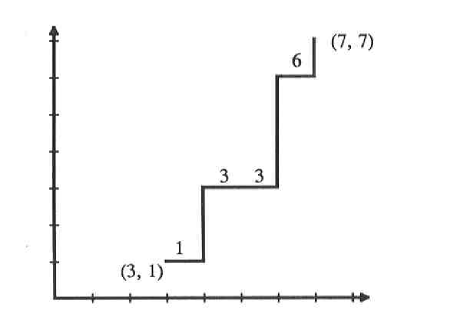
Figure 2: A typical directed random walk

In this figure $Hor_{y}$(P)={1,3,3,6} and, accordingly, w(P)=$x_{1}^{1}x_{3}^{2}x_{6}^{1}$. Next, we need to extend this result to an assembly of directed random walks (”vicious” random walkers in terminology of Fisher [52]). That is we need to consider the products of the type w(P${}_{1})\cdot\cdot\cdot$w(P${}_{k})\equiv$W$($P̂). Finally, the generating function for an assembly of such vicious walkers is given by

$$h_{b-a}(x_{1},...,x_{N})=\sum\limits_{\text{\^{P}}}\text{W}(\text{\^{P}})$$ (1.32)

where W(P̂) is made of monomials of the type $x_{1}^{m_{1}}x_{2}^{m_{2}}...x_{N}^{m_{N}}$ provided that $m_{1}+\cdot\cdot\cdot+m_{N}=b-a.$ The following theorem is proven in Ref.[42,51]

Theorem 1.11. Given integers 0 $<a_{1}<...<a_{k}$ and $0$ $<b_{1}...<b_{k}$ , let M_i,j be the $k\times k$ matrix

$$\text{M}_{i,j}=h_{b_{j}-a_{i}}(x_{1},...,x_{N}),$$ (1.33)

then,

$$\det\text{M=}\sum\limits_{\text{\^{P}}}\text{W}(\text{\^{P}}),$$ (1.34)

where the sum is taken over all sequences (P${}_{1},...,$P${}_{k})=$P̂ of non-intersecting lattice paths P${}_{i}:$ ($a_{i},1)\rightarrow(b_{i},N).$

Corollary 1.12. Put now $a_{i}=i$ and $b_{j}=\lambda_{i}+j$ in Eq.(1.33) provided that  $1\leq i,j\leq k$ with $\lambda$ being partition of $N$ with $k$ parts then, $\det$M=S${}_{\lambda}(x_{1},...,x_{N}).$

Theorem 1.11. provides desired connection between the vicious random walkers and the $\tau$ function of KP hierarchy.

1.5 Organization of the rest of this paper

In Section 2 we provide some facts from the theory of random vicious walkers using results of Fisher [52], Huse and Fisher [53] and Forrester [54].We argue that these results can be obtained also with help of the Bethe ansatz method applied to one dimensional non ideal Bose gas. Such observation is helpful for developing connections between the Yang-Baxter equation, symmetric functions and Schubert polynomials. The obtained Bethe ansatz wave function is reinterpreted in terms of the Gaussian unitary ensemble of random matrices. Using some results for random matrices summarized by Mehta [55] and more recent results by Tracy and Widom [56] (and Forrester [57]) we discuss relations between the Kontsevich matrix Airy integral and that coming from the Gaussian unitary ensemble. We argue that both integrals are tau functions of KP hierarchy. Moreover, we demonstrate that these integrals are actually tau functions for KdV hierarchy of equations (that is they are only a special case of KP hierarchy) and, hence, both can be used as solutions of the W-K model. The arguments of Section 2 are too general. They do not contain explicit reference to 2+1 gravity, moduli space, etc. This deficiency is corrected in Sections 3 and 4 which contain new combinatorial proof of the main identity obtained by Kontsevich [9]:

$$\sum\limits_{\Sigma d_{i}=3g-3+n}<\tau_{d_{1}}\cdot\cdot\cdot\tau_{d_{n}}>_{g}\prod\limits_{i=1}^{n}\frac{(2d_{i}-1)!!}{\lambda_{i}^{2d_{i}+1}}=\sum\limits_{G\in\Gamma_{g,n}}\frac{2^{-\mathcal{V}(\Gamma)}2^{\mathcal{E}(\Gamma)}}{\left|Aut(G)\right|}\prod\limits_{e\in\mathcal{E}(G)}\frac{1}{\lambda_{i(e)}+\lambda_{j(e)}}.$$ (1.35)

This identity connects the observables of topological quantum gravity, Eq. (1.2), with averages of the random matrix (Kontsevich) model associated effectively with the ribbon graphs $\Gamma_{g,n}$ representing the combinatorial moduli space $\mathcal{M}_{g,n}^{comb}$ of marked Riemann surfaces of genus $g$. To avoid repeats of technical details describing random matrices, ribbon graphs, etc., discussed in Sections 3 and 4, we only notice that $\mathcal{V}$($\Gamma)$ in Eq.(1.35) represents the total number of vertices and $\mathcal{E}$($\Gamma)$ the total number of edges of the ribbon graph $\Gamma_{g,n}.$ Mathematically, the identity, Eq.(1.35), is just the statement that there are different but equivalent ways to present partitions discussed in Section 1.4. In section 3 we connect these partitions with some results coming from Nielsen-Thurston theory of surface automorphisms. As it was demonstrated in Refs.[1-4], this theory provides natural mathematical framework for description of dynamics of 2+1 gravity. In these references the canonical (fixed genus $g$) partition function for 2+1 gravity was obtained. This partition function was used for description of the dynamical transition from the pseudo-Anosov to Seifert-fibered (periodic) regime (phase) of 2+1 gravity. We remind our readers about these concepts within the boundaries of Nielsen-Thurston theory. In Sections 3 and 4 we argue that the W-K partition function is relevant for the Seifert-fibered phase. This phase was not discussed in Refs.[1-4]. We should warn our readers that complete description of the Sefert-fibered phase requires more than just the W-K model. For instance, Kulkarni and Raymond [58] had found a very interesting connection between the Seifert-fibered  and anti-de Sitter 3 manifolds which are just Lorentz manifolds of constant negative curvature. Such anti-de Sitter 3 manifolds had been recently classified by Francois [59]. In spite of the fact that they have received considerable attention in physics literature [3] recently, the complete description of this phase ( which by the way contains all known crystallographic groups and much more [60] ) in physical terms remains challenging research problem.

Thus,the results of Refs.[1,4] for the partition function of 2+1 gravity should be extended to reach an accord with results of W-K model. To this purpose, following Nielsen [61], dynamics of the Riemann surface homeomorphisms should be lifted to the universal cover, e.g. to the Poincare’ disc model of H². In such model the set of geodesics (geodesic lamination) is represented by the set of non intersecting arcs (i.e. circular segments whose ends lie on $S_{\infty}^{1}).$The combinatorial arrangement on the disc is described by the Catalan numbers $C_{n}$. These numbers had been used earlier in our work, Ref.[1] for construction of the partition function. In this paper we use this combinatorial data in order to establish several important bijections:1) from the set of arcs to the set of Dyck paths, Fig.5; 2) from the set of Dyck paths to the set of parallelogram polyominoes, Fig.6; 3) from the set of polyominoes to the set of Young tableaux and, finally, 4) from the set of Young tableaux to the set of vicious walkers, Figs.7 and 8. This chain of bijections is needed in order to bring our earlier obtained results for the partition function in accord with the l.h.s. of the Kontsevich identity, Eq.(1.35).To bring this partition function in accord with the r.h.s. of this identity the ribbon graphs need to be constructed. This is discussed in Section 4. Unlike Kontsevich [9] and others [62-64 ], we do not use quadratic differentials (discussed earlier in our papers, Refs.[1,2] ) for construction of these graphs. Our method is based on use of known various equivalent geometrical ways to describe the combinatorics of Catalan numbers [42]. The edges of thus constructed ribbon graphs are replaced by the paths of vicious walkers so that in the end using combinatorics of the Young tableaux the partition function for assembly of vicious walkers acquires the form of the r.h.s. of Eq.(1.35).

Section 5 is included in this work for several reasons. First, it discusses the issue of universality of the W-K model from the point of view of dynamical systems theory. By universality we mean the fact that partition functions of W-K and many related models to be discussed briefly in this section are solutions of the KdV hierarchy. The reasons for this universality can be traced back to the very basic properties of quasiconformal transformations known already to Ahlfors long time ago [65]. Although in Ref. [3] these transformations had been discussed extensively, in this paper more up to date information is presented to make it relevant to the results obtained in earlier sections. This includes some facts about the Thompson and the Ptolemy groups, about their connections with binary trees (and, hence, with Catalan numbers) and their relations with the universal Teichmüller and moduli spaces, etc. Second, it discusses briefly some potential physical and biological applications of the obtained results. Finally, it discusses connections with Frobenius manifolds, self-dual Einstein equations, etc., thus leaving many problems open for further study.

2 From vicious walkers to Kontsevich model via  Gaussian unitary ensemble of random matrices

Following Forrester [54] and Fisher [52], we would like now to formulate a lock step model of vicious walkers. Incidentally, this model is just many walks generalization of the directed polymer model considered in our earlier work, Ref.[66].The continuum limit of the distribution function for this directed polymer produces  the Euclidean version of the Dirac propagator for particle whose mass is associated with bending probabilities to be discussed below. In case of many walkers the fermionic nature of the Dirac ”particles” (walks) imposes a sort of Pauli principle which forbids two walks to intersect. This is characteristic to all quantum many body problems where all ”particles” live in the same ”world time” [67]. In the theory of Brownian motion each walker is allowed to have its own world time [68] so that, accordingly, one can have many  world times quantum mechanics. We shall refrain from discussion of these options referring interested reader to current literature [69]. The lock step model assumes just one ”world time”. Technically this means the following.

We consider a square lattice where $x$ coordinate is assigned for ”space” while the $y$ coordinate is assigned for ”time”. If $p$ walkers are labelled in linear sequence along $x$ axis so that one has

$$x_{1}<x_{2}\cdot\cdot\cdot<x_{p}$$ (2.1)

at ”time” $t=0$, the same inequalities should hold for all subsequent times. The walkers start either on the even or on the odd numbered sites on the x axis. At each tick of the clock each walker moves either to the right or to the left (along lattice diagonals) with equal (bending) probability $w$. The probabilities, in general, may not be equal and are associated with masses of the Dirac particles as discussed in our work, Ref.[66]. Because of imposed initial condition, no two walkers can occupy the same lattice space at any time. This circumstance makes walkers ”vicious”. Let x${}_{0}=(x_{1,0,...,}x_{p,0})$ be the initial configuration of such vicious walkers and x=($x_{1},...,x_{p})$ be the final configuration at time $t$. To calculate the total number of walks starting at $t=0$ at x₀ and ending at $t$at x we need to know the probability distribution $W_{p}(\mathbf{x}_{0}\rightarrow\mathbf{x};t)$ that the walkers proceed without passing, i.e. maintaining the inequalities

$$x_{j-1}(t^{\prime})<x_{j}(t^{\prime})\text{ , }j=2,3,...,p\text{\ for }0\leq t^{\prime}\leq t$$ (2.2)

from their initial configuration at time $t=0$ to their final configuration at time $t$. It is of interest to study this problem for large times: $t\rightarrow\infty$ . In this case it is possible to make a transition to the continuum limit in our study of the probability distribution. In doing so, we shall follow the arguments of Huse and Fisher [53]. To begin, we need to recall that in the continuum limit the probability distribution $W_{p}^{0}(\mathbf{x}_{0}\rightarrow\mathbf{x};t)$ for $p$ independent random walkers is known to be

$$W_{p}^{0}(\mathbf{x}_{0}\rightarrow\mathbf{x};t)=\exp\{-\frac{\left|\mathbf{x}-\mathbf{x}_{0}\right|^{2}}{2Dt}\}/(2\pi Dt)^{p/2}.$$ (2.3)

The diffusion constant $D$ sets up the scale since, as usual, $<$(x${}_{j}-x_{j,0})^{2}>=Dt.$ Because of  use of a single world time for all walkers the above distribution function can be also viewed as distribution function for a single walker in $p$-dimensional Euclidean space. The restrictions  given by Eq.(2.2) impose additional constraints that such a walker must not cross any (hyper)planes described by the set of equations $x_{1}=x_{2},x_{2}=x_{3},...,x_{p-1}=x_{p}$. In view of the results of Section 1, e.g. see Fig.2 and discussion related to it, the assembly of these planes forms Grassmann manifold. This statement can be clarified further by considering the following example. Following Gaudin [70] consider Schrödinger equation for one dimensional Bose gas of $p$ particles interacting via point-like pairvise interaction potential. The dimensionless form of the Schrödinger equation for such particle system is given by

$$-\sum\limits_{i=1}^{p}\frac{\partial_{i}\Psi}{\partial_{i}x^{2}}+2c\sum\limits_{i<j}\delta(x_{i}-x_{j})\Psi=E\Psi.$$ (2.4)

This equation is equivalent to the boundary value problem of obtaining the wave function $\Psi$ of the equation

$$-\Delta_{p}\Psi=E\Psi,$$ (2.5)

where $\Delta_{p}$ is just $p$-dimensional ”free” Laplacian, and the wave function $\Psi$ is subjected to the set of constraints:

$$\left(\frac{\partial}{\partial x_{i}}-\frac{\partial}{\partial x_{j}}\right)\Psi\mid_{x_{i}-x_{j}=0^{+}}=2c\Psi,1\leq i<j\leq p.$$ (2.6)

The condition $\Psi$=0 on the hyperplanes is achieved in the limit $c$=$\infty$ according to Gaudin [70]. It can be shown, that for any $c$ solution of the corresponding quantum mechanical problem is obtained with help of the Bethe ansatz method [70]. Moreover, any problem solvable by the Bethe ansatz method is essentially of the type just described as had been demonstrated rigorously by Gutkin [71]. Therefore, not surprisingly, that there are deep connections between the classical exactly integrable systems of KP type and the quantum mechanical exactly integrable systems solved by the Bethe ansatz method [72]. The Hecke algebra leading to the Yang-Baxter equations providing mathematical justification of the Bethe ansatz method is coming from some particular representation of the symmetric group [73] and, hence, is connected with Schur and related polynomials. Some additional details can be found in Ref. [74].

The mathematical problem posed by Eq.s(2.5) and (2.6) can be equivalently formulated as problem about properties of random walk inside $p-$dimensional caleidoscope. That is we are looking for solution of an eigenvalue problem for ”free ” Laplacian compatible with some reflection group[70,71]. In the simplest cases these are just subgroups of the symmetric group $S_{p}$ made out of even and odd permutations. In view of this, we obtain,

$$W_{p}(\mathbf{x}_{0}\rightarrow\mathbf{x};t)=\sum\limits_{g\in S_{p}}\varepsilon(g)W_{p}^{0}(g\mathbf{x}_{0}\rightarrow\mathbf{x};t),$$ (2.7)

where $\varepsilon(g)=\pm 1$ depending upon the symmetry of permutation (even or odd). Taking Eq.(2.3) into account, this result can be rewritten equivalently as

$$W_{p}(\mathbf{x}_{0}\rightarrow\mathbf{x};t)=U_{p}(\mathbf{x}_{0},\mathbf{x};t)\frac{\exp\{-(\mathbf{x}^{2}+\mathbf{x}_{0}^{2})/2Dt\}}{\left(2\pi Dt\right)^{p/2}},$$ (2.8)

where

$$U_{p}(\mathbf{x}_{0},\mathbf{x};t)=\sum\limits_{g\in S_{p}}\varepsilon(g)\exp\left[(\mathbf{x\cdot}g\mathbf{x}_{0})/Dt\right].$$ (2.9)

Some short calculation explained in Ref. [53] produces

$$U_{p}(\mathbf{x}_{0},\mathbf{x};t)\simeq const\Delta(\mathbf{x})\Delta(\mathbf{x}_{0})/\left(Dt\right)^{n_{p}}$$ (2.10)

with $const=1/1!2!...(p-1)!$ , $n_{p}=\frac{1}{2}p(p-1)$ and $\Delta(\mathbf{x})$ being the Vandermonde determinant:

$$\Delta(\mathbf{x})=\prod\limits_{i<j}(x_{i}-x_{j}).$$ (2.11)

Remark 2.1.  From standard texts in probability theory, e.g. see Ref.[75], it is known that non normalized expression for the probability $W_{p}^{0}(\mathbf{x}_{0}\rightarrow\mathbf{x};t)$ is the long time limit of the formula providing the total number of walks of $n$ steps (since $t\rightleftharpoons n)$ from point x₀  to point x. Accordingly, Eq.s (2.7)-(2.10) provide the total number of nonintersecting directed walks and, hence, $W_{p}(\mathbf{x}_{0}\rightarrow\mathbf{x};t)\approx\det$ M as shown in Eq.(1.34).

It is convenient to assume now that x=x${}_{0}.$ Then, upon rescaling, the following result holds:

$$W_{p}(\mathbf{x=x}_{0};t)\equiv P_{p}(x_{1},...,x_{p})=const\times\exp(-\mathbf{x}^{2})\Delta^{2}(\mathbf{x}).$$ (2.12)

This is just the probability distribution of eigenvalues of random matrices from the Gaussian unitary ensembe [55]. Following Dyson [76]  define the $n-$point correlation function by

$$R_{n}(x_{1},...,x_{n})=\frac{p!}{\left(p-n\right)!}\int\limits_{-\infty}^{\infty}\cdot\cdot\cdot\int\limits_{-\infty}^{\infty}P_{p}(x_{1},...,x_{p})dx_{n+1}\cdot\cdot\cdot dx_{p}.$$ (2.13)

Using this definition the connected $n$-point correlation functions $T_{n}(x_{1},...,x_{n})$ are defined in a usual fashion, e.g.

$$T_{1}(x)=R_{1}(x)$$

$$T_{2}(x_{1},x_{2})=-R_{2}(x_{1},x_{2})+R_{1}(x_{1})R_{2}(x_{2}),$$

etc. Using method of orthogonal polynomials [55] it can be demonstrated that

$$R_{n}=\det[K_{p}(x_{i},x_{j})]_{\mid i,j=1,...,n}$$ (2.14)

where the kernel $K_{p}(x_{i},x_{j})$ is given by

$$K_{p}(x,y)=\sum\limits_{k=0}^{p-1}\varphi_{k}(x)\varphi_{k}(y)$$ (2.15)

with functions $\varphi_{k}(x)$ depending on the random matrix ensemble used. In the case of Gaussian unitary ensemble they are given by

$$\varphi_{k}(x)=(2^{k}k!\sqrt{\pi})^{-\frac{1}{2}}\exp(x^{2}/2)(-\frac{d}{dx})^{j}\exp(-x^{2}).$$ (2.16)

The connected $n$-point correlation function $T_{n}(x_{1},...,x_{n})$ can be neatly represented using the kernel $K_{p}(x,y)$ as follows [55], page 92,:

$$T_{n}(x_{1},...,x_{n})=\sum\limits_{P}K_{p}(x_{1},x_{2})K_{p}(x_{2},x_{3})\cdot\cdot\cdot K_{p}(x_{n},x_{1}),$$ (2.17)

where the sum is over all $(n-1)!$ distinct cyclic permutations of indices $(1,...,n)$. For $p\rightarrow\infty$ the kernel $K_{p}(x,y)$ can be calculated and in terms of the rescaled variables it was obtained independently by Tracy and Widom [56] and by Forrester [57]:

$$K(X,Y)=\frac{Ai(X)Ai^{\prime}(Y)-Ai(Y)Ai^{\prime}(X)}{X-Y},$$ (2.18)

where $Ai(y)$ denotes the Airy function

$$Ai(y)=\int\limits_{-\infty}^{\infty}\exp(i(x^{3}/3-xy))dx$$ (2.19)

and the prime denotes differentiation with respect to its argument. Following Kontsevich [9] we define now the matrix Airy function analogous to the ”scalar” case

$$A(\mathbf{Y})=\int\exp(i\text{ }tr(\mathbf{X}^{3}/3-\mathbf{XY}))\mathbf{dX}$$ (2.20)

where $\mathbf{X}$ and $\mathbf{Y}$ are hermitian $N\times N$ matrices for some $N.$ After some computation Kontsevich obtains,

$$A(\mathbf{Y})=\left(2\pi\right)^{N(N-2)/2}\frac{\det(A^{(j-1)}(Y_{i}))}{\det(Y_{i}^{j-1})},$$ (2.21)

where

$$A^{(j-1)}(y_{i})=\int\limits_{-\infty}^{\infty}dxx^{j-1}\exp(i(x^{3}/3-xy_{i}))=\left(i\frac{\partial}{\partial y_{i}}\right)^{j-1}Ai(y_{i}).$$ (2.22)

For $i,j=1-2$ we obtain,

$$A(X,Y)/(2\pi)^{1/2}=K(X,Y),$$ (2.23)

that is the Tracy-Widom kernel and the Kontsevich Airy matrix integral are practically identical. Naturally, it is of interest to find out if this result will hold for $i,j>2$. Comparing Eq.s. (2.14),(2.17) and (2.23) we conclude, that Eq.(2.17) should be considered as a likely candidate for further treatment. This conclusion is in accord with recent results of Okounkov [77]. We shall use some of his results below in Section 3 while in this section we would like to discuss different approach. To this purpose, following Mehta [55] , let us notice that correlation function $R_{n}$ , Eq.(2.13), can be presented in the following form

$$R_{n}=\sum\limits_{P}(-1)^{n-m}\prod\limits_{1}^{m}K_{p}(x_{a},x_{b})K_{p}(x_{b},x_{c})\cdot\cdot\cdot K_{p}(x_{d},x_{a})$$ (2.24)

where the permutation $P$ is a product of $m$ exclusive cycles of lengths $h_{1},h_{2},...,h_{m}$ of the form ($a\rightarrow b\rightarrow c\rightarrow\cdot\cdot\cdot\rightarrow d\rightarrow a),\sum\nolimits_{1}^{m}h_{j}=n.$ Comparison between Eqs.(2.17) and (2.24) indicates that if, say, the connected $n-$point correlation function $T_{n}$ is tau function of KP hierarchy, then correlation function $R_{n}$ should possess this property as well.

To prove that both $R_{n\text{ }}$and $\ T_{n}$ are indeed tau functions several steps are required. First, we would like to reconsider Eq.(2.21) in the light of subsequent refinements of Kontsevich work in physics literature. Following Di Francesco [78] the Kontsevich integral $\Theta_{N}(\Lambda)$ is given by

$$\Theta_{N}(\Lambda)=\frac{\int e^{tr(i\frac{M^{3}}{6}-\frac{\Lambda M^{2}}{2})}dM}{\int e^{-tr\frac{\Lambda M^{2}}{2}}dM},$$ (2.25)

where $\Lambda$ is diagonal $N\times N$ real matrix with elements $\lambda=(\lambda_{1},...,\lambda_{N})$ along the diagonal and $M$ being $N\times N$ Hermitian matrix. After some calculations this integral can be brought to the following form:

$$\Theta_{N}(\Lambda)=\frac{\left|z,Dz,D^{2}z,...,D^{N-1}z\right|}{\left|1,\lambda,\lambda^{2},...,\lambda^{N-1}\right|},$$ (2.26)

where

$$z=z(\lambda)=\int\limits_{-\infty}^{\infty}dm\sqrt{\frac{\lambda}{2\pi}}\exp\left[i(\frac{m^{3}}{6}+\frac{m\lambda^{2}}{2}-\frac{\lambda^{3}}{3})\right],$$ (2.27)

and

$$D=\lambda+\frac{1}{2\lambda^{2}}-\frac{1}{\lambda}\frac{d}{d\lambda}.$$ (2.28)

The Vandermonde determinant $\Delta(\lambda)$, e.g. see Eq.(2.11), is written in the present case as

$$\Delta(\lambda)=\left|1,\lambda,\lambda^{2},...,\lambda^{N-1}\right|$$ (2.29)

so that the expression in the numerator of Eq.(2.26) is also a determinant. Second, since $z(\lambda)$ is a solution of Airy’s equation

$$\left(D^{2}-\lambda^{2}\right)z(\lambda)=0$$ (2.30)

written in a somewhat unconventional form, it is possible to replace terms of the type $D^{2p}z(\lambda)$ in the determinant of Eq.(2.26) by $\lambda^{2p}z(\lambda)$ and, analogously, $D^{2p+1}z(\lambda)$ by $\lambda^{2p+1}\bar{z}(\lambda)$ where

$$\bar{z}(\lambda)=\frac{1}{\lambda}Dz(\lambda).$$ (2.31)

This allows us to rewrite $\Theta_{N}(\Lambda)$ in the following form

$$\Theta_{N}(\Lambda)=\frac{\left|x^{N-1}z,x^{N-2}\bar{z},....\right|}{\left|x^{N-1},x^{N-2},...,1\right|}$$ (2.32)

with $x=1/\lambda.$ Third, if the asymptotic expansions of $z$ and $\bar{z}$ given by

$$z(\lambda)=\sum\limits_{k\geq 0}c_{k}\lambda^{-3k}$$ (2.33)

$$\bar{z}(\lambda)=\sum\limits_{k\geq 0}d_{k}\lambda^{-3k}$$ (2.34)

with known coefficients $c_{k}$ and $d_{k}$ are substituted into Eq.(2.32) it acquires the following final form:

$$\Theta_{N}(\Lambda)=\sum\limits_{n_{1},...,n_{N}\geq 0}\prod\limits_{i=0}^{N}a_{n_{i}}^{\left(i\operatorname{mod}2\right)}\frac{\left|x^{3n_{1}+N-1}z,x^{3n_{2}+N-2}\bar{z},....,x^{3n_{N}}\right|}{\left|x^{N-1},x^{N-2},...,1\right|}.$$ (2.35)

¿From this form one can recognize at once the Jacobi-Trudy formula [39-42] for the Schur polynomials S_n given as the ratio of determinants. Since Schur polynomials are $\tau$ functions of the KP hierarchy as we had discussed in Section 1, it is clear that $\Theta_{N}(\Lambda)$ is also $\tau$ function of KP hierarchy. Due to specific form of this function (it contains only the odd powers of $\lambda)$ such tau function is actually tau function for the KdV hierarchy in accord with Miwa et all [34]. It remains to demonstrate now that Eq.s(2.17) and (2.24) also can serve as tau functions of KdV hierarchy. Evidently, for $n=2$ this is the case in view of the arguments just presented. To prove that this is the case for $n>2$ it is sufficient to employ the Littlewood-Richardson (”fusion” formula in physics terminology) rule given by

$$\text{S}_{\mu}\cdot\text{S}_{\nu}=\sum\limits_{\lambda}C_{\mu\nu}^{\lambda}\text{S}_{\lambda}$$ (2.36)

with the Littlewood-Richardson coefficients $C_{\mu\nu}^{\lambda}$ assumed to be known [39-42] in principle. Successive applications of this formula to Eq.s(2.17) and (2.24) produces a combination of Schur polynomials each of which is tau function of KP hierarchy. Moreover, since for $n=2$ such tau function was that for KdV hierarchy, evidently, for the same reasons as discussed by Di Francesco [78] the general case $n>2$ also produces tau functions for KdV hierarchy.

3 Nielsen-Thurston surface automorphisms and partition function of 2+1 gravity

3.1 Review of Nielsen-Thurston theory

Let $\mathcal{S}$ be closed orientable Riemann surface of genus $g$.The first homotopy group, the fundamental group $\pi_{1}(\mathcal{S})$ of surface $\mathcal{S}$ is made of $2g$ generators $\{x_{i},y_{i}\}$, $i=1-g$ and a single relation so that its presentation is known to be

$$\pi_{1}(\mathcal{S})=<x_{1},y_{1},...,x_{g},y_{g}\mid[x_{1,}y_{1}]\cdot\cdot\cdot[x_{g},y_{g}]>.$$ (3.1)

Nielsen has noted that there is one to one correspondence between automorphisms of $\pi_{1}(\mathcal{S})$ and surface self-homeomorphisms. This is summarized in the following proposition

Proposition 3.1.(Nielsen [68]) If $g>1$, then every element of $Out$($\pi_{1}(\mathcal{S}))$ is represented by a unique isotopy class of self-homeomorphisms of $\mathcal{S}$.

An important subgroup of $Out$($\pi_{1}(\mathcal{S}))$ is the mapping class group $\mathcal{M}_{g}$ discussed in Section 1. Geometrically, this group is finitely generated by the Dehn twists  in simple closed curves (lamination set) on $\mathcal{S}$ whose physical significance we had discussed extensively in our previous work, Ref.[4].A simple closed curve $\mathcal{C}$ on an orientable surface $\mathcal{S}$ has a neighborhood $\mathcal{E}$ homeomorphic to an annulus which is convenient to parametrize by {[$r$,$\theta$]$\mid$1$\leq r<2\}$.The Dehn twist in $\mathcal{C}$ can be imagined as an automorphism T${}_{C}:\mathcal{S}\rightarrow\mathcal{S}$. It is given by the identity off $\mathcal{E}$ and by [$r$,$\theta$]$\rightarrow[r$,$\theta+2\pi r]$ on $\mathcal{E}$ . Using results of our previous works [1-4], let us illustrate these concepts on the simplest example of a punctured torus T². In this case $Out$($\pi_{1}($T${}^{2}))=GL_{2}(\mathbf{Z})$ and $\mathcal{M}_{1,1}=PSL(2,\mathbf{Z}).$ Since any transformation from $PSL(2,\mathbf{Z})$ is obtainable by projectivisation of $SL(2,\mathbf{Z})$ we discuss everything in terms of $SL(2,\mathbf{Z})$ with projectivisation at the end. Any transformation which belongs to $SL(2,\mathbf{Z})$ is expressible in terms of $2\times 2$  matrix A given by

$$\mathbf{A}=\left(\begin{array}[c]{cc}a&b\\ c&d\end{array}\right)$$ (3.2)

with integer coefficients subject to condition:$\det$A=$ab-cd$=1. The characteristic polynomial for this matrix is given by

$$t^{2}-tr\mathbf{A}\text{ }t+\det\mathbf{A}=0.$$ (3.3)

This implies that the eigenvalues of A are either :

a) both complex ( when trA=0,1,-1),

b) both equal to $\pm 1$ (when trA=$\pm 2),$

c) distinct and real (when $\left|tr\mathbf{A}\right|$ $>$2).

If $\mathfrak{F}_{A}$ is toral automorphism then, transformation a) is called periodic since $\left(\mathfrak{F}_{A}\right)^{n}=1$ for some $n$ (actually, $n=12$ by the Hamilton-Cayley theorem) , transformation b) is called reducible since it leaves a simple closed curve $\mathcal{C}$ invariant, transformation c) is called (pseudo) Anosov ((pseudo)Anosov if the line/vector field on surface (does) does not contain singularities). Such transformations are of an infinite order. Physical significance of this fact is explained and illustrated in our previous work, Ref.[4]. The largest of two eigenvalues is associated with topological entropy of the line/vector flow and is related to the amount of stretching of surface $\mathcal{S}$ and, hence, with the dilatation parameter of the Teichmüller theory.

Nielsen-Thurston theory generalizes the above classification of surface automorphisms to all surfaces of genus $g>1$.Already Nielsen had realized [61] that for $g>1$ it is more convenient to study homeomorphisms of surface $\mathcal{S}$ by considering their image on the universal cover of $\mathcal{S}$ which we choose as Poincare’ disc model of H², i.e. $int$D $\cup$ $S_{\infty}^{1}=$H${}^{2}.$According to Nielsen [61]

Proposition 3.2. Any lift h̃ of  the surface self- homeomorphism h: $\mathcal{S}\rightarrow\mathcal{S}$ to the universal cover of $\mathcal{S}$ extends to a unique self-homeomorphism of the unit disc D, i.e. to intD$\cup S_{\infty}^{1}.$

If surface self-homeomorphisms h are associated with Dehn twists connected with a set of simple closed nonintersecting curves homotopic to geodesics (such set is called geodesic lamination $\mathcal{L}$), then their lifts h̃($\mathcal{L}$) are associated with some maps of the circle $S_{\infty\text{ }}^{1}$extendable (quasi conformally) to the interior of the disc D as discussed in our earlier work Ref.[3] and Section 5. An image of the closed geodesic on $\mathcal{S}$, when lifted to H${}^{2},$ is just a segment of a circle whose both ends lie on $S_{\infty}^{1}$. Since  geodesics are nonintersecting, circle segments on $S_{\infty}^{1}$ are also nonintersecting. In order to recover results of W-K model, in this work we are interested only in the $\mathit{periodic}$ maps of the circle as it will be explained in Section 4 (after Eq.(4.4)). In connection with such maps the following remark is of importance.

Remark 3.3. (A variant of Sarkovskii theorem, Ref.[79], page 88) Let $f$: $S^{1}\rightarrow S^{1}$ be a continuous map of the circle with a periodic orbit of period 3. If the lift $\tilde{f}$: $\mathbf{R}\rightarrow\mathbf{R}$ has also a periodic orbit of period 3 then, $f$ has periodic orbits of every period. The condition on the lift  map f̃ cannot be dropped. In Section 5 we argue that  even though in the case of W-K model the continuous maps of the circle are to be replaced by the piecevise linear maps still 3 remains as minimal period.

Remark 3.4. As noted by Kontsevich [9], moduli space problem makes sense only for Riemann surfaces obeying the following set of inequalities

$$g\geq 0,n>0,2-2g-n<0$$ (3.4)

with $n$ being the number of distinct marked points (effectively distinct boundary components). Boundary components can be eliminated by the Schottky double construction. This construction can be performed as follows. If $M$ is a complex manifold with $C_{1},...,C_{n}$ boundary components, one can consider an exact duplicate of it, say $\hat{M},$ with the same number of boundary components, say, $\hat{C}_{1},...,\hat{C}_{n}.$ Evidently, for each point $x\in M$ there is a ”symmetric” point $\hat{x}\in\hat{M}$ . The Schottky double $2M$ is formed as a disjoint union $M\cup\hat{M}$ and identifying each point $x\in C_{i}$ with point $\hat{x}\in\hat{C}_{i}$ for 1$\leq i\leq n.$ In the simplest case we have initially either punctured torus, i.e.$g=1,n=1$, or the trice punctured sphere, i.e. $g=0,n=3$. In both cases the Schottky double is a double torus. A double torus has 3 geodesics which belong to the geodesic lamination $\mathcal{L}$. The image of these geodesics lifted to H² produces 3 circular arcs whose ends lie on $S_{\infty}^{1}$. This is minimal number of arcs required for the moduli space problem to make sense. According to Remark 3.3. this is also a minimal period for the periodic homeomorphisms of the circle in view of the Sarkovskii theorem. More on this topic will be discussed in Section 5.

In the mean time we would like to discuss the general case of Riemann surfaces of genus $g\geq 1$ with $n$ boundary components. It is argued in Ref.[80] that the total number of geodesics on the Schottky double is $6g-6+3n$. This is the dimension of space of holomorphic quadratic differentials (real on each of the boundary components). Hence, in accordance with Teichmüller theory [20], it is the dimension of the Teichmüller and, accordingly, the moduli space of such Schottky doubled surface.

Remark 3.5. The dimension of moduli space of Schottky doubled surface coincides with the dimension of moduli space $\mathcal{M}_{g,n}^{comb}$ of 3-valent ribbon graphs  used  in Kontsevich paper, Ref.[9]. In the present case the same dimension for the moduli space (as obtained by  Kontsevich) is obtained without explicit use of the quadratic differentials. Moreover, the equivalent of the Kontsevich-Penner ribbon graphs are to be obtained below in Section 4.

It is convenient to map the circle at infinity $S_{\infty}^{1}$ into the real axis R. Accordingly, the arcs corresponding to closed geodesics on the Schottky doubled Riemann surface will become semicircles whose ends are located on the real axis R. This is depicted in Fig.3.

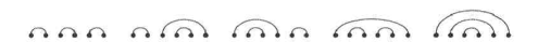
Figure 3: Combinatorics of Catalan numbers presented through arrangements of non intersecting arcs (representing closed hyperbolic geodesics in the upper half plane Poincare model of H${}^{2})$

The mathematical problem associated with arrangement of the arcs depicted in Fig.3 can be formulated according to Stanley [42] as follows: It is required to find a number of ways to connect $2n$ points in the plane lying on a horizontal line by $n$ nonintersecting arcs, each arc connecting two of the points and lying above the points. The solution of this problem is just the Catalan number, $C_{n}=\frac{1}{n+1}\left(\begin{array}[c]{c}2n\\ n\end{array}\right)$. It was used before in connection with construction of the partition function for our 2+1 gravity model [1,2]. Catalan numbers are very helpful in solving the mathematical problem of enumeration of meanders. Meanders had been used as well for description of the partition function of 2+1 gravity [1] and other useful statistical mechanical, dynamical and biological models [81,82]. Meanders can be easily constructed from the double set of arcs as illustrated in Fig.4 taken from our earlier work, Ref.[1].

3.2 Partition function of 2+1 gravity

W-K treatment of 2 dimensional topological quantum gravity is done in the grand canonical formalism. This means that such treatment requires two steps. First, one should construct the (canonical) partition function for the fixed genus Riemann surface. Second, one should perform summation over all genera with some chemical potential. Evidently, the second step can be performed only if the results of the first step are available. For this reason in our previous works [1,2,4] only the first step was considered. Since the main Kontsevich identity, Eq.(1.35), is written for the canonical (fixed genus) case, it is sufficient to consider the fixed genus case in this work also. In order to reach an agreement with W-K results, it is necessary to reconsider our earlier obtained results for the canonical partition function of 2+1 gravity.

Let us begin with some reminders. Meander of order $n$ is a closed nonselfintersecting curve which intersects some straight line in exactly $2n$  preassigned points. In Ref.[1] we had discussed the way meander can be constructed from 2 arc systems, e.g. like those depicted in Fig.3. For reader’s convenience we reproduce a fragment of such construction in Fig.4.

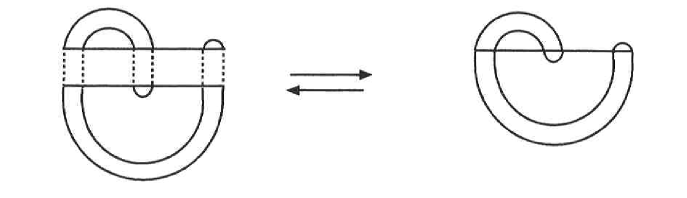
Figure 4: Construction of a typical meander

It is clear from this figure that, in general, such procedure of constructing meanders will yield a set of disconnected meanders. For a given fixed number $n$ let the number $M_{n}^{(k)}$ denote the total number of  disconnected  topologically distinct meanders whose total number is $k$. It is clear, that 1$\leq k\leq n$, and that

$$C_{n}\leq M_{n}\leq C_{n}^{2}$$ (3.5)

where $M_{n}=M_{n}^{(k=1)}.$ Each meander configuration has some statistical weight $x$=$\exp\{-\beta J\}$ (with $\beta$ being some fictitious inverse temperature and J is related to the surface energy) dictated by the physics of the problem [1,4] so that the total canonical partition function $Z(x)$ is given by

$$Z_{g}(x)=\sum\limits_{n=0}^{\infty}x^{n}\sum\limits_{k=1}^{n}M_{n}^{(k)}g^{k}$$ (3.6)

with $g$ being determined implicitly through the equation

$$<k>=g\frac{\partial}{\partial g}\ln Z_{g}(x)$$ (3.7)

with $<k>$ denoting the average number of meanders in the cluster $k.$This number is expected to be assigned. If this is not the case, the partition  function should be written differently.

Remark 3.6. The partition function $Z_{g}(x)$ is written for the system of meanders forming a measured foliation on a Riemann surface $\mathcal{S}$ of fixed genus $g$. Being guided by the Proposition 3.2., we would like to consider the lift of such foliation to the universal cover of $\mathcal{S}$ , i.e. to  the unit disc model of H².

Remark 3.7. In both Ref.[1] and Ref.[4] the main interest in obtaining the partition function was to study dynamical transition from the pseudo-Anosov ( hyperbolic) to periodic (Seifert- fibered) regime. In the present case only the periodic(i.e.Seifert fibered) regime is studied. This is explained in Section 4. Seifert fibered regime is not discussed in Refs.[1,4]. Only in this ( periodic) regime W-K  results can be recovered from 2+1 gravity.

To construct the partition function on the unit disc, it is convenient to map the unit disc into the upper half plane model for H². Then, the system of arcs representing geodesics on $\mathcal{S}$ is mapped into that depicted in Fig.3. Next, the arc system depicted in Fig.3  is mapped  into the associated random walk as depicted in Fig.5.

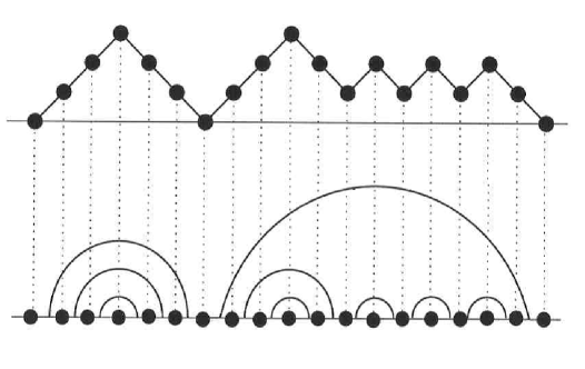
Figure 5: A typical Dyck path [42] from (0,0) to (2n,0) made of steps (1,1) and (1,-1) never falling below x-axis is in one to one correspondence with a typical arrangement of arcs.

Because of such mapping, it becomes possible to connect the combinatorics of vicious walkers discussed in Section 2 with that of arcs and meanders. Indeed, the walk depicted in Fig.5 is directed and is not allowed to intersect $x$ axis, except at initial and final points. By analogy with Fig.4 one can think about another Dyck walk (below $x$ axis). Since both walks intersect each other only at initial and final points this situation looks almost the same as for two vicious walkers. Following Labelle [83], we can make it identical to that for the vicious walkers. To achieve this goal, it is sufficient to translate the upper part by the vector (1,1) while the lower part by the vector (1,-1) so that one obtains either a problem about statistics of one vicious walker in the presence of the absorbing wall or about statistics of two vicious walkers. Both problems are discussed in Fisher’s paper [52] and are actually equivalent. Hence, results of Section 2 can be applied now and one obtains the Tracy-Widom kernel, Eq.(2.18), in the asymptotic limit of large genus or large number of boundary components. This is obviously not sufficient. To go beyond this simple minded result requires to make several nontrivial mappings (bijections). We shall be brief  in describing these bijections since details of the proofs can be found in the published literature.

We begin with the observation that to each Dyck path, e.g. that in Fig.5, one can associate the Dyck word so that the Dyck path having length 2n is encoded by a Dyck word of length 2n. The word is composed of letters x and x̄ in such a way that each North-East (respectively South-East) step correspond to the letter x (respectively x̄). The peaks (respectively troughs) correspond to the factors xx̄ (respectively x̄x). Instead of North-East (respectively South-East) steps it is possible to choose strictly North (respectively East) steps for the Dyck paths to get a configuration like that depicted in Fig.2. Hence, we obtain the following set of bijections: a) from the set of arcs to the set of Dyck paths; b) from set of Dyck paths to the set of Dyck words; c) from the set of Dyck words to the set of lattice paths from $(0,0)$ to $(n,n)$ with steps $(0,1)$ or $(1,0)$ never rising above the line $x=y$ ( incidentally one can construct instead the lattice paths which never go below the diagonal $x=y$ [84] ).To this set of bijections we need to add two more now. The first one is between the Dyck path, e.g. that depicted in Fig.5, and the parallelogram polyomino. Polyomino can be made out of squares (called cells). A finite connected union of cells such that the interior is also connected and there are no cut points is called parallelogram polyomino. It is defined with accuracy up to translation. As depicted in Fig.6,

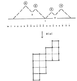
Figure 6: Bijections between the Dyck path, the Dyck word and parallelogram polyomino

a parallelogram polyomino is bordered by two non-intersecting paths having only North and East steps. Fig.6 depicts bijections between the Dyck path, the Dyck word w and parallelogram polyomino $\beta($w). In such bijection the magnitude and the order of peaks and troughs determine the shape of the polyomino [85]. Parallelogram polyomino is in one to one correspondence with skew Young (or Ferres) diagram of shape $\lambda/\mu$ . In the example displayed in Fig.6 we have the shape (4,4,4,2,2,1)/(3,2). That is from standard looking Young table of shape (4,4,4,2,2,1) a piece in the upper left corner is truncated which is also standard table of shape (3,2). Hence, the skew Young diagrams differ very inessentially from standard looking Young diagrams. Using this circumstance, we need to exhibit yet another bijection. It is the most important for our development. To this purpose we need to use the Theorem 1.11. and Corollary 1.12. in order to state yet another

Theorem 3.8. There is a weight -preserving bijection $\varphi$ between non-intersecting paths (P${}_{1},...,$P${}_{k})$ and column strict Young tableaux of shape $\lambda$ with entries from N.

To demonstrate that this is indeed the case, we follow the example discussed in Ref.[51] .More general case of skew column strict Young diagram is discussed in Ref.[42](section 7.16). Following Ref.[51] we take $k=4$, $\lambda=(5,3,2,2)$ and N=6. Although we have now 4 nonintersecting paths their trajectories are completely specified by labeling of their horizontal edges (y-coordinates), e.g. see Fig.2. The information about the path P_k+1-i   can be placed (encoded) into the row $i$ of tableau T. In our case the (vicious) paths are depicted in Fig.7

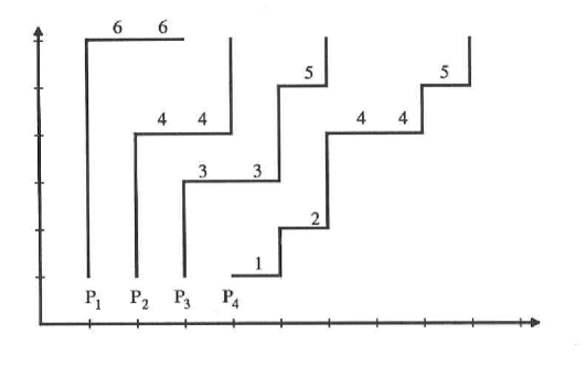
Figure 7: Four vicious walkers encoded by their horizontal edges

while the corresponding encoding of the Young table is depicted in Fig.8. Thus, using results of Section 1, especially Theorem 1.11 and Corollary 1.12, we obtain the determinant det M which contains all the configurational information about collection of vicious walkers.

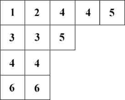
Figure 8: The Young tableau which encodes the information about trajectories of vicious walkers

Using results of Section 2 this information is being translated into that for $n$-point correlation functions $R_{n},$ Eq.(2.24), and $T_{n},$ Eq.(2.17). Using this information and by analogy with Eq.(3.6) the partition function can be written in the following tentative form:

$$Z[\mathbf{x}]=\sum\limits_{n=1}^{\infty}\int\prod\limits_{i=1}^{n}dy_{i}\exp(\mathbf{x}\cdot\mathbf{y})T_{n}[\mathbf{y}]\equiv\sum\limits_{n=1}^{\infty}Z_{n}(\mathbf{x}),$$ (3.8)

where, the boldface for $x$ and $y$ variables reflects the fact that they are multidimensional, e.g. x$\cdot$y=$\sum\nolimits_{i=1}^{n}x_{i}y_{i},etc.$ We use the word ”tentative” because we would like at this point to make a connection with recent works by Okounkov [77,86] and Okounkov and Pandharipande [87] who use the asymptotics of Hurwitz numbers to arrive at results similar to our Eq. (3.8). For reasons which will become clear in the next section and for the sake of agreement with these recent works, Eq.(3.8) should be rewritten as follows:

$$Z_{n}[\mathbf{x}]=Z[x_{1},...,x_{n}]=\frac{(-1)^{n+1}\left(2\pi\right)^{\frac{n}{2}}}{\prod\limits_{i}\sqrt{x_{i}}}\mathcal{E}(\frac{\mathbf{x}}{2^{\frac{1}{3}}})$$ (3.9)

with

$$\mathcal{E}(\mathbf{x})=\int\prod\limits_{i}^{n}dy_{i}\exp(\mathbf{x}\cdot\mathbf{y})T_{n}(\mathbf{y}).$$ (3.10)

Remark 3.9. For developments presented in this paper Eq.s (3.9) and (3.10) are actually unnecessary. They are provided, nevertheless, because they are interesting in their own right and, although the initial arguments in these papers are different from ours, the end results, e.g. Eq.(3.10), is in accord with our Eq.(3.8).

The interest in these equations stems from the fact that in the large $n$ limit, Eq.(3.10) acquires familiar in physics literature path integral form. This fact may lead to some new physical applications. Already many physical applications of vicious walker models can be found in papers by Fisher [52] and  by Huse and Fisher [53].

In the present case, using results of Tracy and Widom ( Eq.(4.6) of Ref.[56]) Eq.(2.18) of Section 2 can be rewritten as follows

$$K(X,Y)=\int\limits_{0}^{\infty}dzAi(X+z)Ai(z+Y)$$ (3.11)

with Airy function defined in Eq.(2.19). Using Okounkov’s Lemma 2.6, Ref. [77],

$$\int\limits_{-\infty}^{\infty}dzAi(z+a)Ai(z+b)\exp(xz)=\frac{1}{2\sqrt{\pi x}}\exp(\frac{x^{3}}{12}-\frac{a+b}{2}x-\frac{\left(a-b\right)^{2}}{4x}),$$ (3.12)

Eq.(3.10) can be rewritten as follows:

$$\mathcal{E}(\mathbf{x})=\frac{1}{2^{n}\pi^{\frac{n}{2}}}\frac{\exp\left(\frac{1}{12}\sum\nolimits_{i}^{n}x_{i}^{3}\right)}{\prod\limits_{i}\sqrt{x_{i}}}\int\limits_{0}^{\infty}\prod\limits_{i}^{n}dy_{i}\exp(-\sum\limits_{i=1}^{n}\frac{(y_{i}-y_{i+1})^{2}}{4x_{i}}-\sum\limits_{i=1}^{n}\frac{y_{i}+y_{i+1}}{2}x_{i}),$$ (3.13)

provided that the cyclic boundary condition , $y_{i+1}=y_{1},$ is imposed. This makes the above ”path integral” reminiscent to that for the ring polymer near hard nonpenetrable wall in the presence of some stretching force [67].

To make connections with results of Kontsevich [9] we need to rewrite the partition function $Z[\mathbf{x}]$ as genus expansion:

$$Z[\mathbf{x}]=\sum\limits_{g=0}^{\infty}Z_{g}(\mathbf{x})$$ (3.14)

where, in view of Eq.(1.2),

$$Z_{g}(\mathbf{x})=\sum\limits_{\Sigma d_{i}=3g-3+n}<\tau_{d_{1}}\cdot\cdot\cdot\tau_{d_{n}}>_{g}\prod\limits_{i=1}^{n}x_{i}^{d_{i}}.$$ (3.15)

The question arises immediately about connections of Eq.s (3.14) and (3.15) with Eq.s (3.8)-(3.10). This issue is addressed and treated in Refs.[77,87] and, therefore, there is no need to repeat the arguments presented in these references here. Instead, to reach essentially the same goals we would like to use different arguments in this work.

In Section 1.1. we had noticed that the calculation of tautological averages is effectively equivalent to the calculation of the Weil-Petersson volumes of $\mathcal{\bar{M}}_{g,n}.$ In algebraic geometry there is a Wirtinger formula for such  volume calculations [12]. In connection with Grassmannians and Schubert calculus this formula had been discussed in the fundamental paper by Chern [46]. Wirtinger-like formula is used in Kontsevich paper as well (e.g.see Section 3 of Ref.[9]).Hence, the partition function of two-dimensional topological gravity is effectively the generating function for the Weil-Petersson volumes. In the fixed genus case such volume according to Kontsevich is given by

$$vol_{p^{\ast}}(\mathcal{\bar{M}}_{g,n})=\frac{1}{d!}\int\limits_{\mathcal{\bar{M}}_{g,n}}(p_{1}^{2}c_{1}(\lambda_{1})+\cdot\cdot\cdot+p_{n}^{2}c(\lambda_{n}))^{d}$$ (3.16a)

with $c_{1}$($\lambda_{i})$ being the first Chern class of the $i-$th line bundle, $i=1,...,n$ and $d=3g-3+n$. The above expression  becomes a true volume when in the set $p^{\ast}$ of indeterminates $p^{\ast}=$($p_{1},...,p_{n})$ (arbitrary sequence of positive numbers) each $p_{i}$ is being put equal to one. This is not necessary, however, since the quantity of interest is the product given by Eq.(1.2) which is obtainable anyway with $p_{i}^{{}^{\prime}}$s   being different from one. Hence, the indeterminates actually play a role of an auxiliary variables analogous to $x_{i}$ in Eq.(3.15). The connection with Schur polynomials and, hence, with tau function is clear if one combines Eq.(1.28) and Porteous formula, Eq.(1.27) with Eq.(3.16a). Finally, arguments  presented in Section 2, especially, Eq.(2.36), provide needed justification of Eq.(3.15) since the result, Eq.(3.16), of Kontsevich can be equivalently rewritten as

$$vol_{p^{\ast}}(\mathcal{\bar{M}}_{g,n})=sgn\times\sum\limits_{\Sigma d_{i}=d}<\tau_{d_{1}}...\tau_{d_{n}}>\prod\limits_{i=1}^{n}\frac{p_{i}^{2d_{i}}}{d_{i}!}.$$ (3.16b)

To make connection with the matrix models additional steps are required. For instance, Kontsevich is making a Laplace transform of Eq.(3.16b) in order to obtain

$$\mathcal{L(}vol_{p^{\ast}}(\mathcal{\bar{M}}_{g,n}))(\lambda_{1},...,\lambda_{n})=\sum\limits_{\Sigma d_{i}=d}<\tau_{d_{1}}...\tau_{d_{n}}>\prod\limits_{i=1}^{n}\frac{\left(2d_{i}\right)!}{d_{i}!}\lambda_{i}^{-\left(2d_{i}+1\right)}$$ (3.17)

with $\lambda_{i}$ being the Laplace variable conjugate to $p_{i}$. Taking into account that $(2d_{i})!/d_{i}!=2^{d_{i}}\cdot\left(2d_{i}-1\right)!!$ the overall factor of $2^{d}$ drops out from the main Kontsevich identity, Eq.(1.35). In view of the results of Refs.[77,86,87] and that going to be presented in Section 4, in order to reach an accord with the result of Kontsevich, Eq.(3.17), it is also necessary to perform the Laplace transform on $Z_{g}(\mathbf{x})$ in Eq.(3.15) provided that this expression is properly rescaled. The Laplace transform is obtained then as follows:

$$\mathcal{L}\left(Z_{g}(\mathbf{x})\right)(\xi_{1},...,\xi_{n})=\int\limits_{0}^{\infty}\prod\limits_{i=1}^{n}dx_{i}\exp(-\mathbf{\xi}\cdot\mathbf{x})Z_{g}(\mathbf{x})\frac{1}{\left(2\pi\right)^{\frac{n}{2}}\prod\nolimits_{i=1}^{n}x_{i}^{\frac{1}{2}}}.$$ (3.18)

Application of the formula

$$\int\limits_{0}^{\infty}dyy^{n-\frac{1}{2}}\exp(-sy)=\Gamma(n+\frac{1}{2})s^{-n-\frac{1}{2}}=\sqrt{2\pi}\frac{\left(2n-1\right)!!}{2^{n+\frac{1}{2}}s^{n+\frac{1}{2}}}$$ (3.19)

to Eq.(3.18) produces the expected result:

$$\mathcal{L}\left(Z_{g}(\mathbf{x})\right)(\xi_{1},...,\xi_{n})=\sum\limits_{\Sigma d_{i}=d}<\tau_{d_{1}}...\tau_{d_{n}}>\prod\limits_{i=1}^{n}\frac{\left(2d_{i}-1\right)!!}{\left(2\xi_{i}\right)^{d_{i}+\frac{1}{2}}},$$ (3.20)

where, in order to achieve an agreement with Kontsevich, one needs to make identification: $\lambda_{i}=\sqrt{2\xi_{i}}$ in Eq.(1.35). Clearly, such identification is ultimately connected with rescaling made in Eq.(3.18).The justification of this rescaling is explained in the next section. This is also needed for completion of the proof of Kontsevich identity, Eq.(1.35) of Section 1.

4 Ribbon graphs,Young tableaux and Kontsevich identity

4.1 Construction of ribbon graphs

Ribbon graphs had been invented by Penner [ 62] ( similar construction can be found also in papers by Harer [88] ) for description of the moduli space $\mathcal{M}_{g,n}$ of Riemann surfaces. In physics literature similar construction had been independently developed by Saadi and Zwiebach [63] and later developed in numerous papers by Zwiebach, e.g. see Ref. [89] cited in Kontsevich work, Ref.[9]. Both Zwiebach and Kontsevich use the Jenkins-Strebel quadratic differentials (e.g. see Section 3 of  our earlier work, Ref.[2], for condensed summary of their properties) for construction of the ribbon graphs. In this section we would like to develop alternative method of construction of ribbon graphs which does not require explicit use of quadratic differentials. We would like to explain the rationale for constructing the ribbon graphs in connection with results obtained thus far in this paper. First, the ribbon graphs appear naturally in matrix models for strings [90] and QCD [91]. Hence, they are physically interesting and easily constructible using Feynman-like rules known in quantum field theory [92]. Second, mathematically these graphs are interesting for several reasons : a) they are associated with problem of imbedding of, say, trivalent graphs into Riemann  surface of fixed genus [93] and, since graphs are related to combinatorial group theory [94], this problem is also of group-theoretic interest; b) these graphs are also related to train tracks discussed in our work, Ref.[2]. Because of this connection with train tracks, the number of potential practical applications is expected to be well beyond particle physics as explained in the discussion section of Ref.[2]. Third, and most important for the purposes of this work, they are needed for establishing one-to one correspondence between the topological gravity and the random matrix models of string theory. The aspects of this correspondence are discussed in detail in Ref.[90]. Mathematically, this correspondence is reflected in the Kontsevich identity, Eq.(1.35). Hence, following Kontsevich [9] it is necessary to prove that the r.h.s.of Eq.(1.35) is equal to the l.h.s. In sections 2 and 3 we had demonstrated that the l.h.s of the identity, Eq.(1.35), is associated with the enumeration of  allowed configurations for an assembly of vicious walkers. This problem has been mapped into enumeration of the Young tableau, e.g. see Figs 7 and 8. These pictures provide a geometrical way of describing partitions of  nonnegative integers. Hence, for ribbon graphs we have to find analogous partitions. Evidently, the Kontsevich identity, Eq.(1.35), is just the statement about existence of different but equivalent ways of  describing partitions as had been stated in the Introduction.

To describe partitions associated with ribbon graphs we need to construct such graphs first. To facilitate reader’s understanding, we employ some results on graphs and ribbon graphs from the pedagogically written paper by Mulase and Penkava [64].Ultimately,our way of constructing the ribbon graphs is different from that discussed in this reference since we are not using quadratic differentials.

Definition 4.1. A graph $\Gamma$=($\mathcal{V}$, $\mathcal{E}$ ; i) consists of a finite set of vertices $\mathcal{V}$=($\mathit{V}_{1},...,\mathit{V}_{m})$ and finite set of edges $\mathcal{E}$ together with a map i from $\mathcal{E}$ to the set ($\mathcal{V}\times\mathcal{V}$)/S₂ of unordered pairs of vertices called incidence relation. The quantity

$$a_{ij}=\left|i^{-1}(V_{i},V_{j})\right|$$ (4.1)

is the number of edges connecting vertices $V_{i}$ and $V_{j}$ . The degree (valence) of a vertex $V_{j\text{ }}$ is the number

$$\deg(V_{j})=\sum\limits_{k\neq j}a_{jk}+2a_{jj}$$ (4.2)

which is the number of edges incident to the vertex.

Definition 4.2. A graph isomorphism is a pair ($\alpha,\beta)$ of bijective maps $\alpha:\mathcal{V}\rightarrow\mathcal{V}^{\prime}$and $\beta:\mathcal{E}\rightarrow\mathcal{E}^{\prime}$ that preserve the incidence relation.

To construct a ribbon graph the above definitions should be modified. The modification consists in labeling of middle points of each edge thus effectively creating extra degree 2 vertices associated with each edge. We denote this extra vertex set as  $\mathcal{V}_{\mathcal{E}}.$ Now the new set of vertices is the disjoint union $\mathcal{V}\sqcup\mathcal{V}_{\mathcal{E}}$ while the new set of edges is the disjoint union $\mathcal{E}\sqcup\mathcal{E}$ since the midpoint of each edge now divides it into two parts. The incidence relation is described now by the map

$$i_{\mathcal{E}}:\mathcal{E}\sqcup\mathcal{E}\longrightarrow\mathcal{V}\times\mathcal{V}_{\mathcal{E}}$$ (4.3)

because each edge of $\Gamma_{\mathcal{E}}$ is connecting one vertex of $\mathcal{V}$ to one vertex of $\mathcal{V}_{\mathcal{E}}$ .Obviously, an edge of $\Gamma_{\mathcal{E}}$ is called a half edge of $\Gamma.$ For every vertex V$\in\mathcal{V}$ of $\Gamma$ , the set i${}_{\mathcal{E}}^{-1}(\{V\}\times V_{\mathcal{E}})$ consists of half edges incident to V so that

$$\deg(V)=\left|i_{\mathcal{E}}^{-1}(\{V\}\times V_{\mathcal{E}})\right|$$ (4.4)

Definition 4.3. A ribbon graph is a graph $\Gamma$=($\mathcal{V}$, $\mathcal{E}$; i) together with a cyclic ordering on the set of half-edges as depicted in Fig.9.

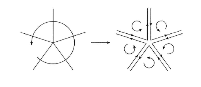
Figure 9: A cyclic ordering at the vertex of the ribbon graph as compared with no ordering in the case of a vertex for ordinary graph

Such definition of the ribbon graph leads to the following construction of such graph out of ordered vertices. The strips corresponding to the two half edges are connected following the orientation of their boundaries to form ribbons. The final surface is no longer planar in general. It is an oriented surface whose boundaries are made of boundaries of the ribbons. To illustrate this construction, let us consider the simplest case first. To this purpose, we recall that for the case of punctured torus and trice punctured sphere we have 3 geodesics (on the Schottky doubled surface) which we lift to the Poincare disc. We associate with these geodesics a trivalent graph as depicted in Fig.10.

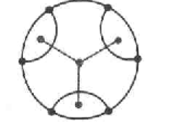
Figure 10: An elementary 3 valent vertex associated with geodesics lifted to the Poincare disc

Next, we make another copy of this picture. Then, we thicken the edges emanating from the vertices and provide orientation in accord with Fig.9. Next, we glue the strips to each other. This can be done in two ways. One is depicted in Fig.11

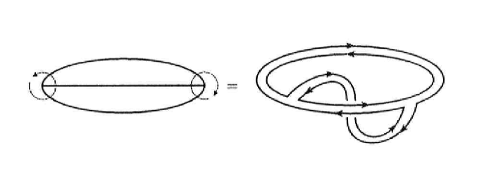
Figure 11: One way to make the simplest ribbion graph (the underlying ”normal” graph is shown for comparison) which is topologically equivalent to the punctured torus. Notice, that the same underlying ”normal” graph also gives rise to another ribbon graph which is topologically equivalent to the trice punctured sphere (not to be confused with that depicted in Fig.12).

while the other is depicted in Fig.12.

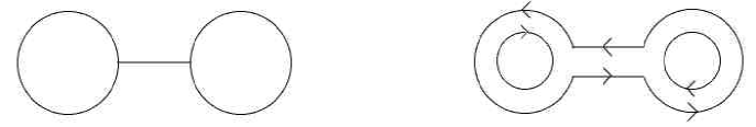
Figure 12: Another way of making the simplest ribbon graph (the underlying ”normal” graph is also shown for comparison). The ribbon graph is topologically eqivalent to the trice punctured sphere

We would like to notice that in both cases we have constructed ribbon graphs $\Gamma_{g,n}=\Gamma$ with the number of thickened edges equal to $6g-6+3n$ number of edges (e.g. 3 for both the trice punctured sphere and the punctured torus) in accord with Kontsevich [9].To obtain more complicated graphs it is convenient to proceed by induction. To this purpose, following again Ref.[64], we need to define the operations of contraction and expansion.

Definition 4.4. If the edge E of $\Gamma$ is incident to two distinct vertices V₁ and V₂ another ribbon graph $\Gamma^{\prime}$ called contraction of $\Gamma$ is obtained from $\Gamma$ by removing the edge E and joining the vertices V₁ and V₂ to a single vertex with the cyclic ordering at the joint vertex determined by the cyclic order of the edges incident to V₁starting with the edge following E up to the edge preceding E, followed by the edges incident to V${}_{2\text{ }}$starting with the edge following E and ending with the edge preceding E.

Evidently, the contraction procedure decreases the number of edges and vertices by one. Every ribbon graph can be obtained from the trivalent ribbon graph by applying a sequence of contractions.

Definition 4.5. The expansion of the ribbon graph is operation  inverse to the contraction.

This means that every trivalent ribbon graph can be constructed by the expansion procedure starting from a very simple analogue of Fig.10. In view of the Euler equation

$$\mathcal{V}(\Gamma)-\mathcal{E}(\Gamma)=2-2g-n$$ (4.5)

such procedure will produce the desired Kontsevich-type trivalent ribbon graph. Let us consider this construction in some detail. For example some representative contraction and expansion of an edge  is depicted in Fig.13 .

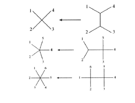
Figure 13: Typical contraction-expansion (Whitehead) moves characteristic for W-K model

Remark 4.6. The reader familiar with our earlier work, Ref.[1], can easily recognize the Whitehead moves characteristic for train tracks. This fact alone is sufficient for making connection between ribbon graphs and quadratic differentials. Since in the present case no topology changing moves are involved, this justifies our earlier statement that the results of W-K can be recovered from the Seifert-fibered (periodic) phase of 2+1 gravity.

For any vertex of degree $d\geq 4$ there are $d(d-3)/2$ ways of expanding it by adding an edge. Consider a portion of $\Gamma$  made of vertex of degree $d\geq 4$ and $d$ half edges emanating from this vertex. A dual to this portion is a convex polygon of $d$ sides depicted in Fig.14 along with the underlying vertex.

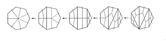
Figure 14: Expansion/contraction of a representative vertex facilitated by the associated with it dual polygon

The series of contractions/expansions is ultimately related to the number of ways a convex polygon with $d$ sides can be triangulated by nonintersecting diagonals. This number is Catalan number again [42]. Although one may probably use this observation to develop bijections analogous to those discussed in Section 3, we leave such an opportunity outside the scope of this work in view of another options to be discussed below.

To finish our construction of the ribbon graphs we have to keep in mind few additional facts. First, by looking at Fig.10 and realizing that two copies of the disc model of H² are needed for construction of the ribbon graph, it is clear that the process of expansion and gluing of strips to each other should be allowed to be different in each disc. Hence, we have to associate the probability of 1/2 to every vertex on each disc. This means that we have to have an overall (assembly) factor of 2^-V(Γ)  for a particular realization of the ribbon graph. Second, the rest of the automorphisms of the ribbon graph are, evidently, the same as for the ”normal” graph.

This concludes our description of the ribbon graph construction.

4.2 Young tableaux and Kontsevich identity

In section 3 the Laplace transform, Eq.(3.20), of the partition function for an assembly of vicious walkers has been obtained. Now it is time to explain how these vicious walkers reemerge with help of the ribbon graphs. To this purpose let us notice that the boundary components of these graphs can be looked upon as made of polygons as Kontsevich had noted in section 2.2. of Ref.[9]. Hence, each ribbon graph is can be classified by certain  non negative integer number of triangles (n${}_{3})$, quadrangles (n${}_{4})$, pentagons (n${}_{5})$, hexagons (n${}_{6})$, etc. Each edge $E_{i}$($\Gamma)$ of the ribbon graph has some length $l_{i}$. Evidently, these lengths can be grouped into sets identified with polygons so that the numbers above represent the multiplicities for these sets. Suppose, that the total length L of all polygons is prescribed in advance. Then, given ribbon graph can be viewed as particular realization of the partition of L into numbers associated with lengths of these polygons. Alternatively, one can assign the total number of polygons (that is the total number of faces n in Eq.(4.5)) and consider partition of this number into n₃, n₅, n${}_{6\text{ }},$ etc. In any case, this means that the Young tableaux can be associated with such partition and, in view of the results of Section 3, again, the vicious walkers can be linked with such Young/Ferrers tables. The question remains: how to connect the vicious walkers with ribbon polygons explicitly? To this purpose recall Remark 2.1. and discussion which follows. According to this remark and the following discussion both correlation functions $R_{n}$ and $T_{n}$ are defined in fact for vicious walks made out of loops. Topologically, our polygons are also loops. Hence, it makes sense to identify the loops entering into expressions for $R_{n}$ and $T_{n}$ with those coming from polygons associated with ribbon graphs. This identification requires some care (that is it requires some proofs) and, hence, cannot be made straightforwardly as we would like to demonstrate now.

If we associate (replace) the polygonal paths by the paths of vicious walkers then, except at vertices, only ”binary interactions” between these walkers need to be considered. These ”binary interactions” are of geometrical origin since they are effectively equivalent to considering just one vicious walker in the presence of an absorbing wall [52]. According to Fisher [52], this means that ”no walk can penetrate the wall and any walk attempting to do so is eliminated”. In addition to the geometrical constraint on such walk, the present case differs from that discussed by Fisher because one has to demonstrate that the walk which survived encounter with one wall entirely forgets about this encounter when it is facing the next wall. Fortunately, this is the case. Indeed, the non normalized distribution function $Q_{n}(x;\sigma)$ for the walk starting at $x=a$ and after $n$ steps reaching the point $x$ is obtained by Fisher, e.g. see Eq.(5.5) of Ref.[52], and is given by

$$Q_{n}(x;\sigma)\approx\frac{e^{-\sigma n}}{\sqrt{\frac{\pi}{2}}}\frac{ax\exp(-\frac{x^{2}}{2n})}{n^{\frac{3}{2}}},$$ (4.6)

where, apart from the factor $aexp(-\sigma n),$one can easily recognize the probability of the first passage through $x$ at ”time” n for the random walk which had started at the origin: $x=0$ [75].This probability has yet another interpretation more suitable for the problem we are discussing. Indeed, following Feller, Ref.[75],Chr3, the same expression describes probability for two dimensional (directed) random walkers which had begun their walk at the origin and after $n$ steps had ended at some point $x>0,y>0$  of $x,y$- plane, provided that these walkers never cross the $x-$ axis. Evidently, one may associate $x-$axis with ”time” (in our case n) direction while $y$ -axis with ”space” direction in order to get vicious walk interpretation of such random walk. In any event, it should be clear that in space direction (that is perpendicular to the wall) such walk is acting as random and, hence, it ”forgets” its past. This observation provides justification for representation of the ”circular” vicious walk by a  sequence of independent random vicious walkers- one for each edge of the closed polygon.

Next, we have to find an analogue of the partition function, Eq.(3.8).This is accomplished in several steps. First, we notice that Eq.(3.8) does not contain information about the number of steps in the walk, only about the number of walks. Using Eq.s (3.8) and (4.6) we introduce for each edge the following generating function (known as perimeter measure [86,87] )

$$C(\xi_{1},\xi_{2})=\int\limits_{0}^{\infty}dxP(\xi_{1},\xi_{2};x)$$ (4.7)

where

$$P(\xi_{1},\xi_{2};x)=\int\limits_{0}^{\infty}dn_{1}\int\limits_{0}^{\infty}dn_{2}Q_{n_{1}}(x;\xi_{1})Q_{n_{2}}(x;\xi_{2})$$ (4.8)

and we put $a=1$ in $Q_{n}(x;\xi)$ in Eq.(4.6). This is permissible since the factor $exp(-\sigma n)$ can be always amended to absorb $a$ (e.g. read Fisher’s paper, Ref.[ ] ). Using Eqs (4.6)-(4.8) the explicit form of the perimeter measure can be easily obtained using standard tables of the Laplace transform. The final result is given by

$$C(\xi_{1},\xi_{2})=\frac{2}{\sqrt{2\xi_{1}}+\sqrt{2\xi_{2}}}.$$ (4.9)

This result should be applied to all edges of the ribbon graph and the final result should take into account all automorphisms $\left|Aut\Gamma\right|$ of the underlying ”normal” trivalent graphs. Taking into account the assembly factor of 2^-V(Γ) the final result can be written as follows

$$\mathcal{L}\left(Z_{g}(\mathbf{x})\right)(\xi_{1},...,\xi_{n})=\sum\limits_{G\in\Gamma_{g,n}}\frac{2^{-\mathcal{V}(\Gamma)}2^{\mathcal{E}(\Gamma)}}{\left|Aut(G)\right|}\prod\limits_{e\in\mathcal{E}(G)}\frac{1}{\sqrt{2\xi_{i(e)}}+\sqrt{2\xi_{j(e)}}}$$ (4.10)

with indices $i$ and $j$ referring to $i$-th and $j-$th polygons sharing the same edge.

Since the l.h.s. is given by Eq.(3.20), Eq.(4.10) coincides with Kontsevich identity, Eq.(1.35), provided that identification $\lambda_{i}=\sqrt{2\xi_{i}}$ is made. Since for trivalent graphs $\left|\mathcal{V}\right|=\frac{2}{3}\left|\mathcal{E}\right|$ , we obtain

$$2^{-\mathcal{V}(\Gamma)}2^{\mathcal{E}(\Gamma)}=2^{2g-2+n}$$ (4.11)

in accord with Ref.[87].

5 Piecewise linear homeomorphisms of the circle and KdV

In this section we would like to provide another interpretation to the results obtained in previous sections. This interpretation is desirable since its aim is to explain to what extent W-K model is universal from the point of view of dynamical systems theory. This is also desirable for the purpose of  connecting results of this paper with WDVV equations and Frobenius manifolds [27,95].  To begin, we need to introduce some information about the Thompson groups.

5.1 Some facts about the Thompson groups

The groups $F$, $T$ and $V$ were introduced by Richard Thompson in 1965. Unfortunately, his results had not been published. This, nevertheless, had not stopped line of research initiated by Thompson as can be seen from the pedagogically written review article by Cannon, Floyd and Parry [96]. Below, we provide some basic facts on Thompson groups using mainly this reference. Additional sources will be used whenever they are needed to suit our needs.

Let $F$ be the set of piecewise linear homeomorphisms from the closed unit interval [0,1] to itself that are differentiable except at finitely many points. Let $f\in F$ and let $0=x_{0}<x_{1}\cdot\cdot\cdot<x_{n}=1$ be the set of points at which $f$ is not differentiable. This partition determines intervals [$x_{i-1},x_{i}]$ for $i=1,...,n$ which are called intervals of the partition. A partition of [0,1] is called standard dyadic partition if and only if the intervals of partition are standard dyadic intervals.

Definition 5.1. A standard dyadic interval in [0,1] is an interval of the form [$\frac{a}{2^{n}},\frac{a+1}{2^{n}}]$ where $a$ and $n$ are nonnegative integers with $a\leq 2^{n}-1.$

It is useful to associate a finite ordered rooted binary tree associated with standard dyadic intervals as depicted in Fig.15.

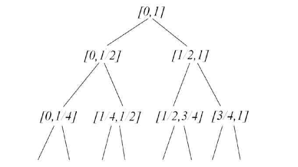
Figure 15: The tree of standard dyadic intervals

For $x_{i-1}\leq x\leq x_{i},i=1,...n,$ the function $f$ can be written as follows

$$f(x)=a_{i}x+b_{i}$$ (5.1)

with $a_{i}$ being a power of 2 and $b_{i}$ being a dyadic rational number. It can be shown that $f^{-1}\in F$ and $f$ maps the set of dyadic rational numbers bijectively to itself. Hence, $F$ is closed under the composition of functions and therefore is a subgroup of the group of all homeomorphisms from [0,1] to [0,1]. This group is $F$ group of Thompson.

Definition 5.2. When points 0 and 1 are identified to make a circle $S^{1}$, then, the resulting Thompson group is called $T$ group. Another Thompson group acting on the circle is $V$ group. Its definition is a bit technical [96] but, at ”physical level” of rigor, the difference between $V$ and $T$ groups is hardly noticeable. Therefore, following Ref.[97] we shall denote both $V$ and $T$ groups as PL${}_{2}(S^{1})$ and we shall keep in mind that both groups are subgroups of the group $Homeo_{+}$ of piecewise orientation-preserving homeomorphisms of the circle. The following proposition proven in Ref.[96] is very important.

Proposition 5.3. Let $f\in F$. Then there exists a standard dyadic partition $0=x_{0}<x_{1}\cdot\cdot\cdot<x_{n}=1$ such that $f$ is linear on every interval of the partition and $0=f(x_{0})<f(x_{1})\cdot\cdot\cdot<f(x_{n})=1$ is a standard dyadic partition.

Evidently, using the proof of this proposition, the same statements can be made for Thompson groups $T$ and $V$ .

Remark 5.4.Using results of Ref.[42], the tree depicted in Fig.15 can be put in bijective correspondence with the set of non intersecting arcs depicted in Fig.3. In view of Proposition 5.3., different arc configurations correspond to different piecewise linear homeomorphisms of the circle caused by PL${}_{2}(S^{1})$. This statement is going to be examined further below in Section 5.3.

Remark 5.5. In view of Eq.(5.1) it can be shown [98] that, except for points $0=x_{0}<x_{1}\cdot\cdot\cdot<x_{n}=1,$ the group PL${}_{2}(S^{1})$ is isomorphic to group PSL${}_{2}(\mathbf{Z})$ which had been discussed at length in our previous work, Ref.[4].

5.2 Some facts about the Ptolemy group

In addition to isomorphism mentioned in Remark 5.5. there is yet another important isomorphism between the Thompson and the Ptolemy groups which we would like to describe briefly in this subsection. Following Lochak and Schneps [99] define the standard marked tessellation of the Poincare disc as dyadic tessellation with marked (oriented) edge from 0 to $\infty$ as depicted in Fig.16.

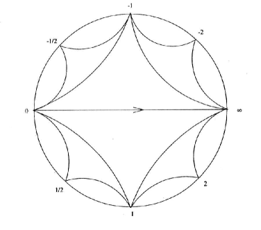
Figure 16: The standard dyadic tesselation of the Poincare disc with oriented marked edge being displayed

The elementary move $\alpha$ on the oriented edge of the dyadic tessellation changes its location from one diagonal of the unique quadrilateral containing it to another one by turning it counterclockwise as depicted in Fig.17.

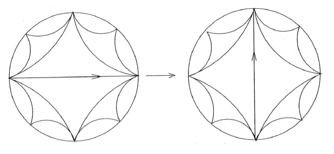
Figure 17: The elementary move on the oriented edge

Such elementary move is of order 4 evidently. In addition to this move there is an arrow-moving move $\beta$ depicted in Fig.18.

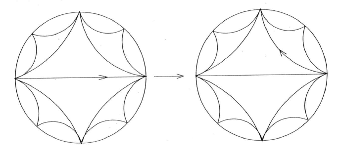
Figure 18: An arrow-moving move

This operation moves an oriented edge to another edge without changing the tessellation itself. The minimal order of this operation is 3. This fact  makes it formally similar to that coming from Sarkovskii theorem, e.g. see Remark 3.3, which forbids periodic orbits of period lesser than 3.Generators $\alpha$ and $\beta$ along with relations

$$\alpha^{4}=1;\beta^{3}=1;\left(\alpha\beta\right)^{5}=1$$ (5.2)

and commutator relations

$$[\beta\alpha\beta,\alpha^{2}\beta\alpha\beta\alpha^{2}]=1;[\beta\alpha\beta,\alpha^{2}\beta\alpha^{2}\beta\alpha\beta\alpha^{2}\beta^{2}\alpha^{2}]=1$$ (5.3)

define the Ptolemy group [99].Imbert had demonstrated [97] that this group is isomorphic to PL${}_{2}(S^{1}).$ The same result is obtained in Ref.[99] with help of slightly different methods.

5.3 Circular homeomorphisms, combinatorics of the ribbon graphs and volumes of hyperbolic polyhedra

Now we would like to add some important details to Remarks 5.4.and 5.5 made above. In view of the Remark 5.5. the standard dyadic tessellation of the Poincare disc depicted in Fig.16 can be shown [97,98] to be in one to one correspondence with the Farey tessellation of the unit disc D discussed in detail in Ref.[4]. Such tessellation can be obtained from two ”seeds”, that is from two triangles with vertices located at 0=1/0, 1=1/1 , $\infty=1/0$ and 0,-1 and $\infty$ respectively (e.g. see Fig.16 and Section 2 of Ref.[4]) The duals to the tessellations originating from these seeds are rooted binary trees whose roots are connected to each other as depicted in Fig.9 of Ref.[4]. The Farey tessellation is also known as ideal triangulation of D [98]. Ideal since the triangle which cover the hyperbolic plane/disc are ideal in the same sense as Euclidean equilateral triangles covering the entire plane without gaps form an ideal triangulation of the Euclidean plane. Since the Farey tessellation is multileveled (e.g. Fig.16 depicts just two levels while Section 2 of Ref.[4] describes how to construct tessellations of any level). If the level is finite(or at least periodic as depicted in Fig.8 of Ref.[4]), then the duals of these tessellations are two rooted binary trees that are also finite. With help of Ref.[42] they can be put in bijective correspondence with two systems of arcs, e.g. those depicted in Figs.3, and 10, etc. needed for construction of the finite ribbon graph as discussed in Section 4. Surely, the infinite level case of Farey tessellation is obtained as limiting case of  finite level case. The moves depicted in Fig.s 17 and 18 are in fact homeomorphisms of the circle [98,100] belonging to the subgroup $Homeo_{+}$. They affect the pattern of triangulation of the unit disc and, hence, affect the binary trees. As demonstrated in Ref.[96], the group of automorphisms of the reduced binary trees ( meaning of the word reduced is explained in Section 2 of Ref.[96].) coincides with Thompson group PL${}_{2}(S^{1}).$ In the same reference the analogue of moves $\alpha$ and $\beta$ for trees is obtained. Some additional physics can be associated now with these mathematical facts. To this purpose, following Ref.[101] we notice that the automorphisms of two binary trees associated with two arc systems are independent. Each of these trees is in bijective correspondence with some triangulation of the convex polygon by non crossing diagonals [42]. Every automorphism of individual tree causes some change in the triangulation pattern for given polygon. Since these changes are independent, following Sleator, Trajan and Thurston [102 ] one may ask about the minimal number of automorphic steps needed to bring one triangulation pattern in exact correspondence with another. This problem is of major importance in computer science. To make it also of importance to physics (and also to evolutionary genetics [103], dynamics and thermodynamics of folding of RNA [82,104], etc.) following Ref.[102 ] several more steps are required. First, by gluing these two polygons to each other we form a triangulated sphere $S^{2}$. Second, we project this sphere stereographically into the complex plane so that pattern of triangulations on $S^{2}$ is transferred to the Euclidean plane. Next, we associate this plane with boundary of the upper half space model for H${}^{3}.$The triangular pattern on such plane is sufficient for reconstruction of the hyperbolic polyhedra according to Thurston [16]. A pedagogical account of how it can be actually done can be found in Ref.[105 ]. Finally, if needed, such polyhedra can be mapped into the hyperbolic ball model of H³ so that the vertices of these hyperbolic polyhedra are located at the sphere at infinity $S_{\infty}^{2}.$ Each triangulation pattern on the sphere $S_{\infty}^{2}$ thus associated with some hyperbolic polyhedron of finite volume $V_{H}$ which is determined by this triangulation pattern. The physics can be now injected into this picture by introducing some Boltzmann factor exp(-$\beta V_{H})$ so that different volumes are related to different triangulations. The larger the volume is for a given ”temperature”$\beta$ , the more stable triangulation pattern becomes. Incidentally, Ref.[102 ] is devoted to finding hyperbolic polyhedra with large volumes.

Remark 5.6. Very recently  statistical mechanics  of various physical systems with Boltzmann factor containing volume (including hyperbolic volume) had been considered by Atiyah and Sutcliffe [106 ]. Actually, these authors had considered instead of volume its logarithm.

5.4 Universal Teichmüller space, KdV and Frobenius manifolds

Connections between the Dyck paths, Virasoro characters and exactly solvable lattice models had been known for some time [107 ].Moreover, since combinatorics of the Dyck paths is directly associated with that for the Catalan numbers, such connections are actually not totally unexpected since there are about 150 interpretations of the Catalan numbers [42]. This, by the way, means that potentially there are much more applications of the W-K model than we had mentioned so far. It is not the purpose of  this subsection to provide the list of such applications. Instead, we are interested in intrinsic features of W-K model which are encoded by the Thompson (or the Ptolemy) group. Following Penner [98,100], the universal Teichmüller space $\mathcal{T}_{ess}$   is defined by

$$\mathcal{T}_{ess}=\frac{Homeo_{+}}{M\ddot{o}b}$$ (5.4)

where $M\ddot{o}b$ is just $PSL(2,R)$.If $\mathcal{T}_{ess^{{}^{\prime}}}$ is a set of all tessellations of D, then $\mathcal{T}_{ess}=\mathcal{T}_{ess^{{}^{\prime}}}/M\ddot{o}b$ as well, as Penner shows. In Section 7 of Ref.[3] we had introduced and discussed the universal Teichmüller space T(1) as defined by Bers. More explicitly, such space is defined by

$$\text{T(1)=}\frac{QS}{PSL(2,R)}$$ (5.5)

with QS being a set of all quasisymmetric deformations of the circle $S_{\infty}^{1}$ (or real line R).We shall discuss these deformations in some detail below. In the meantime we notice that ”physical” definition of the Teichmüller space T is given by

$$\text{T=}\frac{Diff_{+}}{PSL(2,R)}$$ (5.6)

where G= $Diff_{+}$ denote set of all orientation preserving diffeomorphisms of $S_{\infty}^{1}.$ Since G is proper subgroup of QS [98] , it is clear that T is embedded into T(1). In Ref.[98] Penner argues that QS is subset of $Homeo_{+}$ . This leads to the following inclusions:

$$\text{T}\subset\text{T(1)}\subset\mathcal{T}_{ess}.$$ (5.7)

This result is very nontrivial since it makes sense out of  Sarkovskii theorem (Remark 3.3 and Section 5.2) in the present context. It also allows to use Nag and Verjovsky [108] arguments (summarized in Section 7 of Ref.[3]) for use of QS deformations of $S_{\infty}^{1}$ in order to obtain the Virasoro algebra. It is well documented fact that the method of coadjoint orbits [109] directly  connects the Virasoro algebra with KdV equation. The connection between QS deformations and KdV can be established directly without method of coadjoint orbits. For this purpose we need to use some classical results of Ahlfors [65].

Let $w=f(z)$ be a homeomorphism of the complex $z$-plane (or $S^{2}).$Then,

$$dw=f_{z}dz+f_{\bar{z}}d\bar{z}.$$ (5.8)

The complex dilatation factor $\mu$ giving rise to the Beltrami equation is defined now as

$$f_{\bar{z}}=\mu f_{z}$$ (5.9)

and the associated modulus of this dilatation factor is defined by $d_{f}=\left|\mu\right|\leq 1.$The mapping is considered to be $K$-quasiconformal if there is a nonnegative constant $K$ such that $D_{f}\leq K$ ,where $D_{f}=\frac{1+d_{f}}{1-d_{f}}.$ Accordingly, the mapping is conformal if $D_{f}=1.$Suppose now that $f$ maps the upper Poincare half plane to itself (which is, of course, equivalent to the mapping of D to itself). The mapping is quasisymmetric, i.e.$f$ $\in QS$ if for all points $x$, $x-t$ and $x+t$ on real line R the following $M$ condition

$$M^{-1}\leq\frac{f(x+t)-f(x)}{f(x)-f(x-t)}\leq M$$ (5.10)

is satisfied with $M$ being some non negative constant. In Chr.6 of Ref.[65 ] Ahlfors proves that the function which is schlicht and has a quasiconformal extension to the upper half plane must obey the following Fuchsian-type equation known already to Poincare [110]

$$y^{\prime\prime}+\frac{1}{2}\phi y=0.$$ (5.11)

The mapping function $f=y_{1}/y_{2}$ where $y_{1}$ and $y_{2}$ are being two independent solutions of Eq.(5.11) normalized by

$$y_{1}^{\prime}y_{2}-y_{2}^{\prime}y_{1}=1.$$ (5.12)

The function $\phi$ is determined by equation $[f]$=$\phi$ with $[f]$ being the Schwarzian derivative of $f$. Recall [111], that the function is considered to be schlicht (or simple) at some point of complex plane if its first derivative is nonzero at this point.

Lazutkin and Pankratova [112 ] studied Eq.(5.11) from the point of view of the circle maps. They used a variant of Eq.(5.1) given by

$$F(\xi+2\pi)=F(\xi)+2\pi,\xi\in\mathbf{R,}$$ (5.13)

to study the transformational properties of Eq.(5.11). In particular, change of variables

$$x=F(\xi)\text{ and }y\text{(}F\text{(}\xi\text{))=}Y\text{(}\xi)\sqrt{\text{ }F^{\prime}(\xi)}$$ (5.14)

leaves Eq.(5.11) in the same form $Y^{\prime\prime}+\frac{1}{2}\Phi Y=0$ with potential $\Phi$ given by

$$\Phi(\xi)=\phi(F(\xi))\left[F^{\prime}(\xi)\right]^{2}+[F(\xi)]$$ (5.15)

with $[F(\xi)],$ again, being the Schwarzian derivative of $F.$ Eq.(5.15)  actually determines transformational properties of the Schwarzian derivative. In  Ahlfors notations [65] this equation can be equivalently rewritten as equation for transformation of the Schwarzian derivative:

$$[f\circ F]=([f]\circ F])\left(F^{\prime}\right)^{2}+[F].$$ (5.16)

Evidently, this equation holds irrespective to the explicit form of Eq.(5.13).Using this observation it is of interest to consider transformation of the type $F$($\xi)=\xi+\delta\varphi(\xi)$ with $\delta$ being small parameter and $\varphi(\xi)$ some function which makes Eq.(5.13) to hold. Use of this type of function in Eq.(5.16) produces

$$\Phi(\xi+\delta\varphi(\xi))=\phi(\xi)+\delta\left(\hat{T}\varphi\right)(\xi)+O(\delta^{2})$$ (5.17)

with

$$\left(\hat{T}\varphi\right)(\xi)=\phi(\xi)\varphi^{\prime}(\xi)+\frac{1}{2}\varphi^{\prime\prime\prime}(\xi)+\phi^{\prime}(\xi)\varphi(\xi).$$ (5.18)

The Korteweg- de Vries equation can be obtained now in a simple minded way. To this purpose, since $\varphi$ is arbitrary, we choose $\varphi=\phi.$ Next, we make both $\varphi$ and $\phi$ to depend upon the parameter $\delta$ , that is we write $\phi=\phi(\xi,\delta).$Next, we assume that the parameter $\delta$ plays role of ”time” $t$ and, finally, we write

$$\lim_{t\rightarrow 0}\frac{\Phi-\phi}{t}=\frac{\partial\phi}{\partial t}.$$ (5.19)

This then produces our final result:

$$\frac{\partial\phi}{\partial t}=3\phi\phi^{\prime}+\frac{1}{2}\phi^{\prime\prime\prime}.$$ (5.20)

Eq.(5.20) coincides with Eq.(2.2) of Segal [113] and, hence, can be called KdV equation. We provided details of derivation in order to emphasize the universality of this equation in problems which involve circular maps or maps of D. Since KdV is effectively dual to the Virasoro algebra surely it also can be obtained via Nag-Verjovsky approach to construction of the Virasoro algebra and the Kirillov-Kostant two- form by using the universal Teichmüller space T(1) [108 ] . Summary of Nag-Verjovsky results can be found in our earlier work, Ref.[3]. These results were extended by Penner [98] whose Theorem 5.5. essentially assures the existence of the Kirillov-Kostant two form which is invariant under transformation taken from the Ptolemy group. Independent and deep studies of the same problem can be found also in earlier work by Ghys and Sergiescu [114 ]. Higher order KdV can be easily obtained by sequential use of $\hat{T}$ operator as can be seen from Ref.[115 ].

Eq.(5.11) contains actually much more information than we had discussed thus far as was shown by Dubrovin, e.g. see Example C.1.of Ref.[95]. From this example (and preceeding discussion) it follows that variety of  equations of Witten-Dijkgraaf-Verlinde-Verlinde (WDVV) type are obtainable as special cases of Eq.(5.11). Moreover, the self-dual  Yang-Mills and Einstein equations also follow from Eq.(5.11) [95,116]. Geometrically, solutions of WDVV equations represent Frobenius maifolds. Thy are named after Frobenius who was the first to discover them in 1882  [117]. Incidentally, the self-dual Einstein equations had been studied already in 1881 by Halphen [118] and rediscovered by Atiyah and Hitchin [116]. In recent paper by van de Leur and Martini [119] KP representation theory and the related Sato infinite Grassmanian are used to construct solutions of the WDVV equations and, hence, the Frobenius manifolds. In addition, Dubrovin and Zhang [120] had recently demonstrated that , at least for Frobenius manifolds of genus zero and one the Virasoro constraints hold true. That is WDVV equations can be reduced to that of KdV type. This result is in complete accord with arguments provided earlier in this section supporting the claim about universality of KdV type equations. This universality has its origin in the properties of the universal Teichmüller and moduli space. This universality has been studied group-theoretically by Schneps and Lochak [99] who studied action of the Grotendieck-Teichmüller group $\hat{G}\hat{T}$ on Ptolemy-Teichmüller groupoid. Recent lecture notes by Bakalov and Kirillov [121 ] contain some additional helpful information. The authors also discuss connections between the Catalan numbers, modular functor,  modular tensor category, Teichmüller tower, Knizhnick-Zamolodchikov equations, etc. and contain many references on latest important related works. The latest paper by Schneps and Nakamura [122] should, perhaps, be added to the list references. It is our hope, that mentioning of all these beautiful mathematical results in this paper may encourage some applications of these results in areas other than mathematics and theoretical particle physics.

Note added in proof.While this paper was under refereing, several important recent publications came to our attention. In particular, Ref.[123] provides a very efficient introduction into Schubert polynomials, Shubert varieties and related topics. Refs.[124,125] written and edited by Gian Carlo Rota provide an indispensable supplement to book by Stanley [42]. These referenses allow to keep things in historical perspective and, hopefully, should serve as an inspiration for many additional potential applications. In recent paper by Sözen and Bonahon [126] it is shown that the Weil Petersson symplectic form $\omega_{w-p}$,e.g. see Eq.(1.4), coincides with Thurston intersection form $\tau$ for geodesic laminations ( more details on this subject can be found from yet unpublished book by Francis Bonahon ”Closed Curves on Surfaces” available on line ).This allows to establish connections between foliations/laminations and non commutative geometry as actually had been demonstrated by Connes [127] some time ago.In addition to monograph [27] by Manin, recently Manin and Zograf  had obtained explicit asymptotics for Weil-Petersson volumes of the moduli spaces of punctured Riemann surfaces in the limit of fixed genus and number of punctures groving to infinity [128] while Grushevsky have obtained the asymtotics for the fixed number of punctures with genus groving to infinity [129]. In Ref.[130] Guha made some progress in showing new connections between the diffeomorphisms of the circle and the exactly integrable systems of the Korteweg-deVries type by connecting them with differential Galois theory. Finally, direct links between the results of our Ref. [4] and those discussed in this paper could be also developed with help of random polynomials [131,132].

Acknowledgment. The autor would like to thank Bojko Bakalov (MIT), Andrei Okounkov (U. of California, Berkeley) and Igor Rivin (Temple U.) for stimulating correspondence. In addition, the author would like to thank Motohico Mulase(U.California, Davis) and Michael Penkava (U.of Wisconsin-Eau Claire) for granting permission to reproduce Figures # 9, 11, 13 and 14 in this work.

References

[1] A.Kholodenko, Use of meanders and train tracks for description of

defects and textures in liquid crystals and 2+1 gravity,

J.Geom.Phys.33 (2000) 23-58.

[2] A.Kholodenko, Use of quadratic differentials for description of defects

and textures  in liquid crystals and 2+1 gravity,

J.Geom.Phys.33 (2000) 59-102.

[3] A.Kholodenko, Boundary conformal field theories, limit sets of Kleinian

groups and holography, J.Geom.Phys.35 (2000) 193-238.

[4]  A.Kholodenko, Statistical mechanics of 2+1 gravity from Riemann zeta

function and Alexander polynomial:exact results,

J.Geom.Phys.38 (2001) 81-139.

[5] E.Witten, Two-dimensional gravity and intersection theory on moduli

space, Surveys in Diff.Geom.1 (1991) 243-310.

[6] J.Harris, I.Morrison, Moduli of Curves, Sringer-Verlag,

New York, 1998.

[7] E.Looijenga,Cellular decompositions of compactified moduli spces of

pointed curves, in R.Dijkgraaf,C.Faber,G.Vander Geer $\left(\text{Eds.}\right)$,

The Moduli Space of Curves, Birkhäuser, Boston, 1995, pp.369-400.

[8] R.Hain, E.Looijenga, Mapping class groups and moduli spaces of curves,

Proc.Symp.Pure Math. 62 (1997) 97-142.

[9] M.Kontsevich, Interrsection theory on the moduli space of curves and

the matrix Airy function,Comm.Math.Phys.147 (1992) 1-23.

[10] Y.Namikawa, A conformal field theory on Riemann surfaces realized

as quantized moduli theory of Riemann surfaces, Proc.Symp.Pure Math.

49(1) (1989) 413-443.

[11] M.Dunajski, L.Mason, P.Tod, Einstein-Weil geometry, the dKP

equation and twistor theory, J.Geom.Phys.37 (2001) 63-93.

[12] P.Griffiths, J.Harris, Principles of Algebraic Geometry,

John Willey & Sons, New York, 1994.

[13] V.Danilov, V.Shokurov, Algebraic Curves, Algebraic Manifolds

and Schemes, Springer-Verlag, New York, 1998.

[14]  C.McMullen, Renormalization and 3-Manifolds which Fiber over the

Circle, Princeton U.Press, Princeton, 1996.

[15] P.Deligne, D. Mumford, The irreducibility of the space of curves of

given genus, Inst. Hautes etudes Sci.Publ.Math. 45 (1969) 75-109.

[16] W.Turston, Geometry and Topology of 3-Manifolds, Princeton

University Lecture Notes,1979 http://www.msri.org/gt3m/

[17] W.Thurston, On the geometry and dynamics of diffeomorphisms of

surfaces, Bull.AMS (N.S.) 19 (1988) 417-431.

[18] K.Matsutaki, M.Taniguchi, Hyperbolic Manifolds and Kleinian Groups,

Clarendon Press, Oxford, 1998.

[19] S.Wolpert, On the homology of the moduli space of stable curves,

Ann.Math.118 (1983) 491-523.

[20] Y.Imayoshi, M.Taniguchi, An Introduction to Teichmüller Spaces,

Springer-Verlag, New York, 1992.

[21] E.D’Hoker,D.Phong, The geometry of string perturbation theory,

Rev.Mod.Phys.60 (1988) 873-916.

[22] S.Wolpert, On the Kähler form of the moduli space of once

punctured tori, Comm.Math.Helvetici 58 (1983) 246-256.

[23] R.Penner, Weil-Petersson volumes, J.Diff.Geom.35 (1992) 559-608.

[24] P.Zograf, The Weil-Petersson volume of the moduli space of punctured

spheres, Contemp.Math.150 (1993) 367-372.

[25] M.Matone, Nonperturbative model of Liouville gravity, J.Geom.Phys.

21 (1997) 381-398.

[26] R.Kaufman,Y.Manin, D.Zagier, Higher Weil-Petersson volumes

of moduli  spaces of stable n-pointed curves,

Comm.Math.Phys.181 (1996) 763-787.

[27] Y.Manin, Frobenius Manifolds,Quantum Cohomology, and Moduli Spaces,

AMS Publications, Providenve, RI, 1999.

[28] R.Wells, Differential Analysis on Complex Manifolds, Prentice Hall Inc.,

New York, 1973.

[29] S.Wolpert, On obtaining a positive line bundle from the

Weil-Petersson class, Am.J.Math.107 (1985)1485-1507.

[30] S.Wolpert, The hyperbolic metric and the geometry of universal curve,

J.Diff.Geom. 31 (1990) 417-472.

[31] H.Sato, Algebraic Topology: An Intuitive approach, AMS Publications,

Providence, RI, 1999.

[32] S.Novikov, Topology I, Springer-Verlag, Berlin, 1996.

[33] W.Baily, On the imbedding of V-manifolds in projective space,

Am.J.Math.79 (1957) 403-430.

[34] T.Miwa, M.Jimbo, E.Date, Solitons,Cambridge U.Press,

Cambridge, 2000.

[35] S.Kleiman, D.Laksov, Schubert calculus, Am.Math.Monthly 79 (1972)

1061-1082.

[36] W.Hodge, D.Pedoe, Methods of Algebraic Geometry, Vol.2,

Cambridge U.Press, Cambridge, 1952.

[37] D.Gepner, Fusion rings and geometry, Comm.Math.Phys.141

(1991) 381-411.

[38] E.Witten, The Verlinde algebra and the cohomology of the Grassmanian,

arXiv:hep-th/9312104.

[39] W.Fulton, J.Harris, Representation Theory,

Springer-Verlag, Berlin, 1991.

[40] W.Fulton, Young Tableaux, Cambridge U.Press, Cambridge, 1997.

[41] W.Fulton, Intersection Theory, Springer-Verlag, Berlin, 1984.

[42] R.Stanley, Enumerative Combinatorics, Vol.2 , Cambridge U.Press,

Cambridge, 1999.

[43] I.Porteous, Simple singularities of maps, LNM192 (1971) 286-312.

[44] G.Horrocks, Proc.London Math.Soc.(3) 7 (1957) 265-280.

[45] J.Carrel, Chern classes of the Grassmanians and Schubert calculus,

Topology 17 (1978) 177-182.

[46] S.Chern, Characteristic classes of hermitian manifolds,

Ann.Math. 47 (1946) 85-121.

[47] C.Ehresmann, Sur la topologie de certains espaces homogenes,

Ann.Math.35 (1934) 396-443.

[48] T.Suwa, Indices of Vector Fields and Residues of Singular

Holomorphic Foliations, Hermann, Paris, 1998.

[49] T.Regge,General relativity without coordinates,

Nuovo Cim.19 (1961) 558-571.

[50] S.Chern, Complex Manifolds Without Potential Theory,

Springer-Verlag, Berlin, 1979.

[51] D.Stanton, D.White, Constructive Combinatorics, Springer-Verlag,

Berlin, 1986.

[52] M.Fisher, Walks, walls, wetting and melting, J.Stat.Phys.34

(1984) 667-729.

[53] D.Huse, M.Fisher, Commensurate melting, domain walls, and

dislocations, Phys.Rev.B 29 (1984) 239-269.

[54] P.Forrester, Exact solution of the lock step model of vicious

walkers, J.Phys.A 23 (1990) 1289-1273.

[55] M.Mehta, Random Matrices, Academic Press, New York, 1991.

[56] C.Tracy, H.Widom, Level-spacing distributions and the Airy Kernel,

Comm.Math.Phys.159 (1994) 151-174.

[57] P.Forrester, The spectrum edge of random matrix ensembles,

Nucl.Phys.B402 (1993) 709-728.

[58] R.Kulkarni,F.Raimond,3-dimensional Lorentz space-forms and

Seifert fiber spaces, J.Diff.Geom.21 (1985) 231-268.

[59] S.Francois, Variete’s anti-de Sitter de dimension 3 possedant

un champ de Killing non trivial,C.R. Acad.Sci.,

Paris,Ser.I Math.324 (1997) 525-530.

[60] W.Dunbar, Geometric orbifolds, Rev.Math.

Univ.Madrid 1 (1988) 67-99.

[61] J.Nielsen,  Untershungen zur Topologie der geslossenen

zweiseitigen Flachen I, Acta Math. 50 (1927) 189-358.

[62] R.Penner, The decorated Teichmüller space of punctured surfaces,

Comm.Math.Phys.113 (1987) 299-339.

[63] M.Saadi, B.Zwiebach, Closed string theory from polyhedra,

Ann.Phys.192 91989) 213-227.

[64] M.Mulase, M. Penkava, Ribbon graphs, quadratic differentials

on Riemann surfaces, and algebraic curves defined over Q̄,

Asian J.Math.2 (1998) 875-919.

[65] L.Ahlfors, Lectures on Quasiconformal Mappings,

D.van Nostrand Co.,Inc., New York, 1967.

[66] A.Kholodenko, Fermi-Bose transmutation: from semiflexible polymers

to superstrings, Ann.Phys.202 (1990) 186-225.

[67] A.Kholodenko,Th.Vilgis, Some geometrical and topological problems

in polymer physics, Phys. Reports 298 (1998) 251-370.

[68] K.Ito, H.McKean, Diffusion Processes and Their Sample Paths,

Springer-Verlag, Berlin, 1965.

[69] J.Harlee, Time amd time functions in reparametrized nonrelativistic

quantum mechanics, Class.Quantum Grav. 13 (1996) 361-375.

[70] M.Gaudin, La Function D’Onde De Bethe, Masson, Paris, 1983.

[71] E.Gutkin, Bethe ansatz and the generalized Yang-Baxter equations,

Ann.Phys.176 (1987) 22-48.

[72] I.Krichever, O.Lipan, P.Weigmann, A.Zabrodin, Quantum

integrable models and discrete classical Hirota equations,

Comm.Math.Phys. 188(1997) 267-304.

[73] S.Majid, Foundations of Quantum Group Theory, Cambridge U.Press,

Cambridge, 1995.

[74] S.Fomin, A.Kirillov, The Yang-Baxter equation, symmetric functions,

and Schubert polynomials, Discrete Math.153 (1996) 123-143.

[75] W.Feller, An Itroduction to Probabiliy Theory and Its Applications,

Vol.1, John Wiley &Sons, Inc., New York, 1968.

[76] F.Dyson, Statistical theory of energy levels of complex systems,

J.Math.Phys. 3 (1962) 140-156.

[77] A.Okounkov,Generating functions for intersection numbers on moduli

spaces of curves, arXiv: mathAG/0101201.

[78] P.Di Francesco, 2-d quantum and topological gravities,

matrix models, and integrable differential systems, in

The Painleve Property, Springer-Verlag, Berlin, 1999,

pp.229-285.

[79] W. de Melo, S.van Strien, One-Dimensional Dynamics,

Springer-Verlag, Berlin, 1993.

[80] F.Tomi, A.Tromba, The index theorem for minimal surfaces of

higher genus, AMS Memoirs 117 (1995) 1-78.

[81] P.Di Francesco,O.Golonelli, E.Guttier, Meander, folding and arc

statistics, Math.Comput.Modelling 26 (1997) 97-147.

[82] R.Simion, Noncrossing partitions, Discr.Math. 217 (2000) 367-409.

[83] J.Labelle, On pairs of non-crossing generalized Dyck paths,

J.of Stat.Planning and Inference 34 (1993) 209-217.

[84] J.Fedou, Enumeration of skew Ferres diagrams and basic

Bessel functions, Journ.of Stat.Planning and Inference

34 (1993) 107-123.

[85] M.Delest, G.Viennot, Algebraic languages and polynomioes

enumeration, Theor.Comp.Sci. 34 (1984) 169-206.

[86] A.Okounkov, Random matrices and random permutations,

Int.Math.Res.Notices 20 (2000) 1043-1095.

[87] A.Okounkov, R.Panharipande, Gromov-Witten theory, Hurwitz

numbers, and matrix models, arXiv: math.AG/0101147.

[88] J.Harer, The cohomology of moduli space of curves,

LNM 1337 (1988) 138-221.

[89] B.Zwiebach, How covariant closed string theory solves a minimal area

problem, Comm.Math.Phys.136 (1991) 83-118.

[90] J.Amjorn, B.Durhuus, T.Josson, Quantum Geometry,

Cambridge U.Press,Cambridge, 1997.

[91] W.Taylor, Counting strings and phase transitions in 2d QCD,

arXiv:hep-th/9404175.

[92] D.Bessis, C.Itzykson, J-B Zuber, Quantum field theory techniques in

graphical enumeration, Adv.Appl.Math.1 (1980) 109-157.

[93] A.White, Graphs, Groups and Surfaces, North Holland,

Amsterdam, 1973.

[94] D.Collins, R.Grigorchuk, P.Kurchanov, H. Zieschang ,

Combinatorial Group Theory and Applications to Geometry,

Springer-Verlag, Berlin, 1998.

[95] B.Dubrovin, Geometry of 2d topological field theories,

LNM 1620 (1996) 120-348.

[96] J.Cannon,W.Floyd and W.Parry, Introductory notes on Richard

Thompson’s groups, Enseign.Math.42 (1996)215-256.

[97]  M.Imbert, Sur l’isomorphisme du groupe de Richard Thompson

avec le groupe de Ptolemee’, in :Geometric Galois Actions,

Cambridge U.Press, Cambridge,1997, pp.313-324.

[98] R.Penner, Universal constructions in Teichmüller theory,

Adv.Math.98 (1993) 143-215.

[99]  P.Lochack, L.Schnieps, The universal Ptolemy -Teichmüller groupoid,

in :Geometric Galois Actions, Cambridge U.Press, Cambridge,

1997, pp. 325-347.

[100] R.Penner, The universal Ptolemy group and its completions,

in Geometric Galois Actions, Cambridge U.Press, Cambridge,

1997, pp.293-312.

[101] R.Alperin,W Dicks, J.Porti, The boundary of the Gizeking tree

in hyperbolic three space, Topology.Appl. 93 (1999) 219-259.

[102] D.Sleator, R.Trajan,W.Thurston, Rotation distance, triangulations

and hyperbolic geometry, J.of AMS 1 (1988) 647-681.

[103] M.Yang, Introduction to Statistical Methods in Modern Genetics,

Gordon and Breach Publ., 2000.

[104] R.Penner, M.Waterman, Spaces of RNA secondary structures,

Adv.Math.101 (1993) 31-49.

[105] P.Callahan, A.Reid, Hyperbolic structures on knot complements,

Chaos, solitons and Fractals 9 (1998) 705-738.

[106] M.Atiyah, P.Sutcliffe, The geometry of point particles,

arXiv: hep-th/0105179.

[107] A.Carey, M.Murray, Geometrical Analysis and Lie Theory

in Mathematics and Physics,  Cambridge U.Press,

Cambridge, 1998.

[108] S.Nag, A.Verjovsky, Diff(S${}^{1})$ and the Teichmüller spaces,

Comm.Math.Phys.130 (1990) 123-138.

[109] V.Arnold, B.Khesin, Topological Methods in Hydrodynamics,

Springer-Verlag, Berlin, 1998.

[110] H.Poincare, Papers on Fuchsian Functions,

Springer-Verlag, Berlin, 1985.

[111] H.Cohn, Conformal Mapping on Riemann Surfaces,

Dover Publications, Inc., New York, 1967.

[112] V.Lazutkin, T.Pankratova, Normal forms and versal deformations for

the Hill equation, Funct.Analysis and Appl. 9 (1975) 41-48.

[113] G.Segal, The geometry of the KdV equation,

Int.J.Mod.Phys.A 6 (1991) 2859-2869.

[114] E.Ghys,V.Sergiescu, Sur un groupe remarquable de

diffeomophismes du cercle, comm.Math.Helv. 62 (1987) 185-239.

[115] A.Das, Integrable Models, World Scientific, Singapore, 1989.

[116] M.Atiyah, N.Hitchin, The Geometry and Dynamics of

Magnetic Monopoles, Princeton U.Press, Princeton, 1988.

[117] F.Frobenius,Stickelberger, Uber die Differentiation der

elliptishen Functionen nach den Perioden und Invarianten,

J.Reine Angew. Math.92 (1882).

[118] G.Halphen, Sur un systemes d’equations differentielles,

C.R.Acad. Sc. Paris 92 (1881) 1001-1007.

[119] J. van de Leur, R.Martini, The constructionof Frobenius

manifolds from KP tau-functions, Comm.Math.Phys.

205 (1999) 587-616.

[120] B.Dubrovin, Y.Zhang, Frobenius manifolds and Virasoro constraints,

Sel.Math., New Ser.5 (1999) 423-466.

[121] B.Bakalov, A.Kirillov, Jr., Lectures on Tensor Categories and

Modular Functors, AMS Publ., Providence, R I , 2001.

[122] H.Nakamura, L.Schneps, On subroup of the Grothendieck-Teichmüller

group acting on tower of profinite Teichmüller modular groups,

Inv.Math. 141 (2000) 503-560.

[123] L.Manivel, Symmetric Functions, Schubert Polynomials and

Degeneracy Loci, SMF/AMS Texts and Monographs,

Vol.6, Providence, R.I., 2001.

[124] Gian-Carlo Rota on Combinatorics, Editor J.P.S.Kung, Birkhäuser,

Boston, 1995

[125] Classic Papers in Combinatorics, Edited by I.Gessel and G-C Rota,

Birkhäuser, Boston, 1987.

[126] Y.Sözen, F.Bonahon,The Weil-Petersson and Thurston symplectic

forms, Duke Math.Journal 108 (2001) 581-597.

[127] A.Connes, A survey of foliations and operator algebras, Proc.Symp.

Pure Math.Vol.38, AMS, Providence, R.I.,1982.

[128] Y.Manin, P.Zograf, Invertible cohomological field theories and

Weil-Petersson volumes, arXiv: math. AG/9902051

[129]  S.Grushevsky, An explicit upper bound for Weil-Petersson

volumes of the moduli spaces of punctured Riemann surfaces,

Math.Ann.321( 2001) 1-13.

[130] P.Guha, Diff($S^{1})$ and Adler-Gelfand-Dikii spaces and integrable

systems. lett.in Math.Phys.55 (2001) 17-31.

[131] A.Edelman, E.Kostlan, How many zeros of a random polynomial

are real?, Bull.AMS 32 (1995) 1-37.

[132] E.Bogomolny, O.Bohigas,P.Leboefuf, Quantum chaotic dynamics

and random polynomials, J.Stat.Phys. 85 (1996) 639-679.