hep-th/0111261

Integrable Quantum Field Theories, in the Bulk and with a Boundary

Peter Aake Mattsson

Department of Mathematical Sciences, University of Durham, Durham DH1 3LE, England.

Abstract

In this thesis, we consider the massive field theories in 1+1 dimensions known as affine Toda quantum field theories. These have the special property that they possess an infinite number of conserved quantities, a feature which greatly simplifies their study, and makes extracting exact information about them a tractable problem. We consider these theories both in the full space (the bulk) and in the half space bounded by an impenetrable boundary at $x=0$. In particular, we consider their fundamental objects: the scattering matrices in the bulk, and the reflection factors at the boundary, both of which can be found in a closed form.

In Chapter 1, we provide a general introduction to the topic before going on, in Chapter 2, to consider the simplest ATFT—the sine-Gordon model—with a boundary. We begin by studying the classical limit, finding quite a clear picture of the boundary structure we can expect in the quantum case, which is introduced in Chapter 3. We obtain the bound-state structure for all integrable boundary conditions, as well as the corresponding reflection factors. This structure turns out to be much richer than had hitherto been imagined.

We then consider more general ATFTs in the bulk. The sine-Gordon model is based on $a_{1}^{(1)}$, but there is an ATFT for any semi-simple Lie algebra. This underlying structure is known to show up in their S-matrices, but the path back to the parameters in the Lagrangian is still unclear. We investigate this, our main result being the discovery of a “generalised bootstrap” equation which explicitly encodes the Lie algebra into the S-matrix. This leads to a number of new S-matrix identities, as well as a generalisation of the idea that the conserved charges of the theory form an eigenvector of the Cartan matrix.

Finally, our results are summarised in Chapter 5, and possible directions for further study are highlighted.

Note added

The work which follows was presented as a thesis for the degree of Doctor of Philosophy at the University of Durham in September 2000. Since then, Bajnok et al. [62, 63, 64] have also studied the problem of the boundary sine-Gordon model with arbitrary integrable boundary conditions. Their results provide independent confirmation of many of those reported here. We are also grateful to Gabor Takács and Zoli Bajnok, in particular, for pointing out a number of typos in [1]. Since they apply equally to the content of this thesis, we record them here.

• We should perhaps have made it clear that the lemmas presented in Chapter 3 rested on an implicit assumption that, when the the incoming particle decays into two other particles, neither is the outgoing particle. Examples such as Figure 3.7 are therefore technically exceptions to the lemmas as stated. These cases were not discussed explicitly in the text as they are only relevant when the rapidity of the incoming particle is independent of the boundary parameter.

• In equation (3.24) [equation (18) in [1]], the two $l/2\lambda$ terms should read $l/\lambda$.

• Just above Table 3.1 [Table 1 in [1]], $b^{1}_{m,1}$ should read $a^{1;m}_{1}$.

• In Table 3.7 [Table 7 in [1]], the order of the pole at $\nu_{0}$ is not correct; it should be $k$.

The hep-th version of [1] has been updated to incorporate the last three amendments.

Contents

1. Preface
2. 1 Integrable Quantum Field Theory in Two Dimensions
   1. 1.1 Introduction
   2. 1.2 Exact S-matrices
      1. 1.2.1 Yang-Baxter (or “factorisation”) equation
      2. 1.2.2 Unitarity, analyticity and crossing symmetry
      3. 1.2.3 The Bootstrap Principle
      4. 1.2.4 The Coleman-Thun mechanism
   3. 1.3 Boundary field theory
      1. 1.3.1 Boundary Yang-Baxter equation
      2. 1.3.2 Boundary unitarity condition
      3. 1.3.3 Boundary crossing symmetry condition
      4. 1.3.4 Boundary bootstrap
      5. 1.3.5 The boundary Coleman-Thun mechanism
   4. 1.4 Summary
3. 2 Classical sine-Gordon Theory
   1. 2.1 Introduction
   2. 2.2 The bulk theory
   3. 2.3 The theory on the half-line
   4. 2.4 Particle content
   5. 2.5 Construction of boundary bound states
      1. 2.5.1 Notation
      2. 2.5.2 The position problem
      3. 2.5.3 Solving the boundary condition
      4. 2.5.4 The general solution
   6. 2.6 Boundary bound states
      1. 2.6.1 Boundary breathers
      2. 2.6.2 Another bound state
   7. 2.7 Predictions
4. 3 Quantum Boundary sine-Gordon Theory
   1. 3.1 Introduction
   2. 3.2 Review of previous results
      1. 3.2.1 The theory in the bulk
      2. 3.2.2 The theory with a boundary
   3. 3.3 The boundary Coleman-Thun mechanism
   4. 3.4 The Dirichlet case
      1. 3.4.1 The soliton sector
      2. 3.4.2 The breather sector
   5. 3.5 Initial pole analysis
      1. 3.5.1 Solitonic ground state factors
      2. 3.5.2 Solitonic excited state reflection factors
      3. 3.5.3 Breather ground state reflection factors
      4. 3.5.4 Breather excited state reflection factors
   6. 3.6 An example
      1. 3.6.1 Boundary ground state—soliton sector
      2. 3.6.2 Boundary ground state—breather sector
      3. 3.6.3 First level excited states—soliton sector
      4. 3.6.4 First level excited states—breather sector
      5. 3.6.5 Second level excited states—soliton sector
      6. 3.6.6 Second level excited states—breather sector
      7. 3.6.7 Third level excited states—soliton sector
      8. 3.6.8 Third level excited states—breather sector
      9. 3.6.9 Summary
   7. 3.7 The general case
      1. 3.7.1 The minimal spectrum
      2. 3.7.2 Reflection factors for the minimal spectrum
      3. 3.7.3 Solitonic pole structure
      4. 3.7.4 Breather pole structure
   8. 3.8 Number of states
   9. 3.9 Other boundary conditions
      1. 3.9.1 Resonance states
   10. 3.10 Summary
5. 4 Affine Toda Theory
   1. 4.1 Introduction
   2. 4.2 The Lagrangian
   3. 4.3 The Quantum Theory
      1. 4.3.1 Simply-laced cases
      2. 4.3.2 Nonsimply-laced cases
   4. 4.4 Lie algebra structure
   5. 4.5 The consequences
      1. 4.5.1 An integral formula
      2. 4.5.2 A formula for the conserved charges
      3. 4.5.3 Multi-linear Identities
   6. 4.6 Summary
6. 5 Conclusions
   1. 5.1 Introduction
   2. 5.2 Bulk ATFTs
   3. 5.3 Boundary sine-Gordon
7. A Boundary sine-Gordon Details
   1. A.1 Infinite products of gamma functions
   2. A.2 Relation of $M$ and $\varphi_{0}$ to $\eta$ and $\vartheta$
      1. A.2.1 Comparison with other results
   3. A.3 On-shell diagrams
8. B Miscellaneous Proofs
   1. B.1 Oota’s starting point
   2. B.2 The generalised bootstrap at $\theta=0$
   3. B.3 Check that generalised bootstrap follows from integral formula
   4. B.4 Fourier transforms
   5. B.5 Dynkin diagrams
   6. B.6 Cartan matrices for simple Lie algebras
   7. B.7 S-matrices
      1. $g_{2}^{(1)}\quad h=6\mathrm{\ and\ }r^{\vee}h^{\vee}=12$
9. Epilogue

Preface

This thesis is the result of work carried out in the Department of Mathematical Sciences at the University of Durham, between October 1996 and September 1999, under the supervision of Dr. Patrick Dorey. No part of it has been previously submitted for any degree, either in this or any other university.

No claim to originality is made for the review in Chapter 1, nor for the introduction to the sine-Gordon model at the beginning of Chapter 2 or the introduction to ATFTs in Chapter 4. The work on the classical sine-Gordon theory in Chapter 2 is new and due solely to the author. The study of the quantum model with Dirichlet boundary conditions in Chapter 3 was carried out jointly with Patrick Dorey, and has been published as [1]. The extension to arbitrary boundary conditions is again new.

The idea for the work on bulk ATFTs in Chapter 4 emerged from conversations with Patrick Dorey (notably the generalised bootstrap) and with Roberto Tateo (the idea of comparing the generalised bootstrap before and after interchanging indices as a method of generating S-matrix identities). The implementation of these, however, and the motivation behind the bootstrap, is due to the author. Much of this has already been published [2], but the discussion presented here was lacking.

Some of the results presented here have also been obtained by other groups, working independently. In particular, the “generalised bootstrap” identity was found by Fring, Korff and Schultz [3], while some of the S-matrix identities were found in an ad-hoc fashion by Khastgir [4]. In addition, work on the boundary sine-Gordon model with Neumann boundary conditions has been carried out by Brett Gibson.

Acknowledgements: I would like to thank Patrick Dorey for all his help, as well as Roberto Tateo, Andreas Fring, Matthias Pillin, Subir Ghoshal, Gustav Delius, Aldo Delfino and Brett Gibson for interesting discussions. Financial support was provided by the EPSRC (who funded a Research Studentship) and by a TMR grant of the European Commission (reference ERBFMRXCT960012), both of whom I acknowledge and thank.

Finally, thanks are undoubtedly due to Tuki, Adelene and my parents, for valiantly trying—against all odds—to keep me sane, keeping my talent for procrastination in check, and so allowing this thesis to be submitted before the Last Trump, rather than just afterwards as was once feared. I am also deeply grateful to Mr Lee, my erstwhile English teacher, who helped me to believe in myself, and to realise that maybe scientists can write too! (He also asked for my first book to be dedicated to him, without realising the consequences…)

Chapter 1 Integrable Quantum Field Theory in Two Dimensions

“I got really fascinated by these 1+1 models …and how mysteriously they jump out at you and work and you don’t know why. I am trying to understand all this better.”

—Richard Feynman

1.1 Introduction

“‘The time has come,’ the walrus said, ‘to talk of many things. Of ships and shoes and sealing-wax, and cabbages and kings.”’

—Lewis Carroll

Why study a theory in two dimensions, when the real world has at least four? The difficulty, at least at present, is that realistic four-dimensional field theories are incredibly complicated, even before the further dimensions proposed by superstring theories are considered. Perturbative solutions can be found, but exact, non-perturbative, results are few. In a number of cases, sufficiently accurate perturbative answers are enough, but many physical phenomena cannot be properly understood this way. Uncovering exact solutions to quantum field theories is considered by many to be one of the great remaining challenges to particle theorists.

In view of this, it is perhaps logical to think of taking a step backwards, to consider a simpler model which still exhibits some of the same features. Understanding the issues involved a few at a time in this way presents a more manageable problem, like climbing a mountain in stages rather than hoping to stride straight to the top. A theory with two dimensions, one of space and one of time, is a useful starting point.

The main focus of this thesis will be the scattering matrices (S-matrices) of these theories, which describe how the final state of the system is related to the initial state. In general this is a messy object to deal with, since there are potentially matrices for the evolution of any number of particles into any other number. However, the theories considered here are “simplified” in one further respect in that they are integrable theories. This has three main effects:

• there is no net particle production, so the number of particles in the initial and final states must always be the same;

• the outgoing particles must have the same masses and velocities as the incoming ones;

• a general S-matrix, for the scattering of $n$ particles, can always be factorised into a product of two-particle S-matrices.

In essence, this means that, once the S-matrix for the scattering of two particles into two particles has been calculated, everything else follows, making a characterisation of the theory in terms of these matrices a more attractive and tractable proposition.

The method for obtaining explicit expressions for these S-matrices is in fact surprisingly straightforward (if not necessarily simple to put into practice). It invokes four consistency requirements which, between them, provide strong constraints on the S-matrix. This method, first formulated in the 1960s, was initially developed to help explain the strong nuclear force (see e.g. [5, 6]). In the 1970s, it was discovered that these axioms could also be applied to some two dimensional quantum field theories, and proved in certain cases to be powerful enough to completely determine the S-matrix up to an overall factor.

A theory is integrable if it has an infinite number of symmetries; the particular theories we will be studying, the affine Toda field theories (ATFTs), acquire these through being based on an infinite-dimensional Lie algebra. We will study these both in the full 2-dimensional space, and in a half space (or half line) defined by introducing an impenetrable boundary at $x=0$. As well as the usual S-matrices, this requires the introduction of boundary factors to describe particles scattering against the boundary. The particles can either simply reflect from this “wall” or bind to it, and we will be concerned with the bound state structure this introduces.

The situation with a boundary is the less well-understood of the two, so we shall study only the simplest ATFT, the sine-Gordon model. Even for this case, only the ground and first few excited states have been explored. We present a complete description of these matrices, for any wall which leaves the resultant theory integrable.

Without a boundary, the picture is much clearer, and S-matrices have been found for all real-coupling ATFTs. However, despite the manifest Lie algebraic structure of the theory, its path from the Lagrangian to the S-matrix is still not precisely known, and remains an open problem. We will, however, present a convenient way of encoding the Lie algebra into the matrix, with the aim of making the task a little easier. This process will also throw up a number of new relationships between elements of the S-matrix.

Apart from their interest in connection with higher-dimensional theories, two-dimensional integrable models have an increasing number of applications in their own right. They are, for example, useful in studying impurity problems in an interacting 1D electron gas [7] or edge excitations in fractional quantum Hall states [8, 9]. (A recent review can be found in [10].)

In the following sections all this will be put on a more formal basis, paving the way for the discussion of the ATFTs which will occupy our attention for the remainder of the thesis.

1.2 Exact S-matrices

“The three rules of the Librarians of Time and Space are: 1) Silence; 2) Books must be returned no later than the date last shown; and

3) Do not interfere with the nature of causality.”

—Terry Pratchett, Guards! Guards!

Much of the discussion in this section is based on [11, 12, 13]. Before proceeding to specifics, a gentle introduction to two-dimensional field theory is perhaps appropriate.

Let us begin by considering a general Euclidean field theory with one space and one time dimension $(x^{1},x^{2})=(x,t)$ defined (in the Lagrangian approach) by the classical action

$$\mathcal{A}=\int_{-\infty}^{+\infty}dx\int_{-\infty}^{+\infty}dt\,a(\varphi,\partial_{\mu}\varphi),$$ (1.1)

where $\varphi(x,t)$ is some set of fundamental fields and the action density $a(\varphi,\partial_{\mu}\varphi)$ is a local function of these fields and the derivatives $\partial_{\mu}\varphi=\partial\varphi/\partial x^{\mu}$ with $\mu=1,2$. For simplicity we shall also use light-cone coordinates, so that, in place of $(p^{0},p^{1})$ for the two-momentum, we will take $(p,\overline{p})=(p^{0}+p^{1},p^{0}-p^{1})$.

We will be considering the particles only on mass-shell (i.e. real, rather than virtual, particles), which means that their two-momenta satisfy the mass-shell condition

$$p_{a}\overline{p}_{a}=(p_{a}^{0})^{2}-(p_{a}^{1})^{2}=m_{a}^{2},\,(a=1,2,\ldots,n).$$ (1.2)

The two momenta can be conveniently parametrised in terms of their rapidity $\theta$:

$$(p_{a}^{0},p_{a}^{1})=(m_{a}e^{\theta_{a}},m_{a}e^{-\theta_{a}}).$$ (1.3)

Suppose our theory contains $n$ different types of particle $A_{a},a=1,2,\ldots,n$, with masses $m_{a}$. The asymptotic particle states are generated by the “particle creation operators” $A_{a}(\theta)$:

$$|A_{a_{1}}(\theta_{1})A_{a_{2}}(\theta_{2})\cdots A_{a_{n}}(\theta_{n})\rangle=A_{a_{1}}(\theta_{1})A_{a_{2}}(\theta_{2})\cdots A_{a_{n}}(\theta_{n})|0\rangle.$$ (1.4)

Looking into the far past, we shall call the state an in state if there are no further interactions as $t\rightarrow-\infty$. This means that the fastest particle must be on the left, and the slowest on the right, with all the others in order in-between, i.e. $\theta_{1}>\theta_{2}>\cdots>\theta_{n}$. Similarly, if there are no further interactions as $t\rightarrow\infty$, the state will be called an out state, and the rapidities must be in the reverse order.

The S-matrix can now be introduced as a mapping between the in-state basis and the out-state basis. It is useful to consider the $A_{x}(\theta)$s as non-commuting symbols, giving them an existence outside the ket vectors, so that we can write the above state simply as $A_{a_{1}}(\theta_{1})A_{a_{2}}(\theta_{2})\ldots\linebreak A_{a_{n}}(\theta_{n})$. Considering an $m$-particle in-state, we have

$$A_{a_{1}}(\theta_{1})A_{a_{2}}(\theta_{2})\ldots A_{a_{n}}(\theta_{n})=$$ (1.5)

$$\sum_{m=1}^{\infty}\sum_{\theta_{1}^{\prime}<\ldots<\theta_{m}^{\prime}}S_{a_{1}\ldots a_{n}}^{b_{1}\dots b_{m}}(\theta_{1}\ldots\theta_{n};\theta_{1}^{\prime}\ldots\theta_{m}^{\prime})A_{b_{1}}(\theta_{1}^{\prime})A_{b_{2}}(\theta_{2}^{\prime})\ldots A_{b_{m}}(\theta_{m}^{\prime})$$

where a sum on $b_{1}\ldots b_{n}$ is implied, and the sum on the $\theta_{i}^{\prime}$ will, in general, turn out to involve a number of integrals. The rapidities will also be constrained by momentum conservation.

For a general theory, we can proceed no further, and introducing the S-matrix would appear only to have complicated matters. However, for an integrable theory, the whole situation becomes dramatically simpler. The name derives from the classical formulation of such theories, which can be cast as partial differential equations; these were said to be integrable if it was possible to find an explicit solution. It was found that a solution was only possible if there were an infinite number of symmetries constraining the behaviour of the equation, and preventing it from becoming chaotic. The same applies here: possessing so many symmetries constrains the S-matrix sufficiently to allow an exact solution to be found.

Energy-momentum is always a conserved quantity, and its operator, P, is said to have (Lorentz) spin 1 as it transforms under a Lorentz boost $L_{\alpha}:\theta\rightarrow\theta^{\prime}=\theta+\alpha$ as ${\textbf{P}}\rightarrow{\textbf{P}^{\prime}}=e^{\alpha}{\textbf{P}}$. This means that a boost of $2i\pi$—a complete rotation—has no effect. On a one-particle state, the action of ${\textbf{P}}=(P,\overline{P})$ would be

$$P|A_{a}(\theta)\rangle=m_{a}e^{\theta}|A_{a}(\theta)\rangle,\quad\overline{P}|A_{a}(\theta)\rangle=m_{a}e^{-\theta}|A_{a}(\theta)\rangle\,.$$ (1.6)

In general, there can also be other conserved quantities, $\textbf{Q}_{s}$, which transform in higher representations of the 1+1-dimensional Lorentz group as ${\textbf{Q}_{s}}\rightarrow{\textbf{Q}_{s}^{\prime}}=e^{\alpha s}{\textbf{Q}_{s}}$ and have spin $s$ since they rotate $s$ times under a boost of $2i\pi$. This time, the effect of ${\textbf{Q}_{s}}=(Q_{s},Q_{-s})$ on a one-particle state is

$$Q_{s}|A_{a}(\theta)\rangle=q_{a}^{(s)}e^{s\theta}|A_{a}(\theta)\rangle,\quad Q_{-s}|A_{a}(\theta)\rangle=q_{a}^{(s)}e^{-s\theta}|A_{a}(\theta)\rangle\,.$$ (1.7)

In an integrable theory, there are an infinite number of these conserved quantities (or “charges”). It might, at first, appear that such theories are quite improbable. In the theories to be considered later, these symmetries are due to an underlying group structure which happens to be infinite-dimensional.

We will concentrate on local conserved charges, which are those whose operators are integrals of strictly local densities, meaning that their action on multi-particle states is additive:

$$Q_{s}|A_{a_{1}}(\theta_{1})\ldots A_{a_{n}}(\theta_{n})\rangle=(q_{a_{1}}^{(s)}e^{s\theta_{1}}+\ldots+q_{a_{n}}^{(s)}e^{s\theta_{n}})|A_{a_{1}}(\theta_{1})\ldots A_{a_{n}}(\theta_{n})\rangle.$$ (1.8)

Just as, above, momentum conservation constrained the sum over the rapidities, so all the other conserved quantities provide additional constraints, leaving an infinite number of equations to be solved, of the form

$$q_{a_{1}}^{(s)}e^{s\theta_{1}}+\ldots+q_{a_{n}}^{(s)}e^{s\theta_{n}}=q_{b_{1}}^{(s)}e^{s\theta_{1}^{\prime}}+\ldots+q_{b_{m}}^{(s)}e^{s\theta_{m}^{\prime}}.$$ (1.9)

Since these must all hold for all possible sets of in-momenta, the only possible solution is the trivial one, i.e. $n=m$, and $\theta_{i}=\theta_{i}^{\prime}$, $q_{a_{i}}^{(s)}=q_{b_{i}}^{(s)}$ for all $i$.

This establishes the fact that there can be no particle production in an integrable theory, and that the sets of incoming and outgoing momenta must be equal, thus reducing the workload involved in dealing with the S-matrix just to the $n\rightarrow n$ cases. There is, however, one further property of integrable theories which makes them even easier to deal with: factorisation. This states that, for any $n\rightarrow n$ S-matrix, the trajectories of the particles involved can be shifted forwards or backwards in space so as to split the vertex into a product of $\frac{1}{2}n(n-1)$ two-particle vertices, as shown in figure 1.2.

The origin of this property can be seen in the fact that, while the momentum operator, for example, will act on a given state simply by shifting the position of all the particles by a fixed amount, higher-spin operators will, in general, change the positions by an amount depending on the initial momentum of the particle. This argument was first proposed by Shankar and Witten [14] and elaborated by Parke [15]. In rough form it goes as follows.

The first step is to note that, since we are dealing with a local, causal field theory, the particles in any process are sufficiently well separated (at least most of the time) to be considered individually, and it is reasonable to consider the effect of the conserved charges particle by particle. If we consider a single-particle state, with position approximately $x_{1}$ and spatial momentum approximately $p_{1}$, the position space wavefunction will be

$$\psi(x)\propto\int_{-\infty}^{+\infty}dp\,e^{-a^{2}(p-p_{1})^{2}}e^{ip(x-x_{1})}.$$ (1.10)

For simplicity, rather than considering a general spin-$s$ operator, we will now try acting on this with $P_{s}$, the spin $s$ operator which acts as $(P)^{s}$, i.e. as $s$ copies of the spatial part of the two-momentum operator. Applying $e^{-i\alpha P_{s}}$ to the above wavefunction gives

$$\overline{\psi(x)}\propto\int_{-\infty}^{+\infty}dpe^{-a^{2}(p-p_{1})^{2}}e^{ip(x-x_{1})}e^{-i\alpha p^{s}}.$$ (1.11)

Since most of the value of the integral is due to the region around $p\approx p_{1}$, we can Taylor expand the extra factor in powers of $(p-p_{1})$ to find new values for the position and momentum. For a general momentum-dependent phase factor $e^{-i\phi(p)}$, this leaves the momentum unchanged but shifts the position by $\overline{x_{1}}=x_{1}+\phi^{\prime}(p_{1})$. Here, this gives a position shift of $s\alpha p^{s-1}_{a}$. For momentum itself, this is just $\alpha$ but, for higher spins, the shift must depend on the initial momentum. This, as Parke showed, is a general property of higher-spin operators.

Applying a suitable operator, $Q_{s}$, near an $n\rightarrow n$ vertex thus separates the particles and splits up the vertex into $\frac{1}{2}n(n-1)$ $2\rightarrow 2$ vertices. However, since the operator is related to a conserved charge, the amplitude for both processes must be the same, giving us factorisability. In addition, applying $Q_{-s}$ rather than $Q_{s}$ causes a mirror-image split, leading to figure 1.2.

This relies, of course, on the fact that, after splitting up the vertex, the particle trajectories must still cross somewhere, because we are restricted to only two dimensions. In higher numbers of dimensions, it is quite easy to imagine splitting up such a vertex so that the particles never meet at all, leading to a trivial S-matrix. In fact, Coleman and Mandula [16] proved the so-called Coleman-Mandula theorem, showing that, for any theory with more than one space dimension and a conserved charge with spin 2 or more, the S-matrix must be trivial.

All this shows that an integrable theory in 1+1 dimensions is rather special, in that it has:

• no particle production;

• equality of the sets of initial and final momenta;

• factorisability of the $n\rightarrow n$ S-matrix into a product of $2\rightarrow 2$ S-matrices.

With these results, it is clear that the $2\rightarrow 2$ S-matrix is the fundamental object of the theory, and that, once it has been found, the full S-matrix is only a step away. The $2\rightarrow 2$ process is just

$$A_{a_{1}}(\theta_{1})A_{a_{2}}(\theta_{2})=S^{b_{1}b_{2}}_{a_{1}a_{2}}(\theta_{1}-\theta_{2})A_{b_{2}}(\theta_{2})A_{b_{1}}(\theta_{1}),$$ (1.12)

and is shown graphically in figure 1.1. (In this, and in all subsequent diagrams, time is taken to run up the page, and space from left to right.) Note that momentum conservation demands $m_{a_{1}}=m_{b_{1}}$ and $m_{a_{2}}=m_{b_{2}}$, so that $a_{1}\neq b_{1}$ or $a_{2}\neq b_{2}$ are only possible if there is a degenerate mass spectrum.

$=S_{a_{1}a_{2}}^{b_{1}b_{2}}(\theta)$

Figure 1.1: S-matrix

The two-particle S-matrix has $n^{4}$ elements, but these are not all independent, and are in fact strongly constrained. Firstly, it is generally assumed that parity, charge conjugation and time reversal (P, C and T) symmetries hold. These impose the conditions

$$S^{kl}_{ij}(\theta)=S^{lk}_{ji}(\theta)=S^{\overline{k}\overline{l}}_{\overline{\imath}\overline{\jmath}}(\theta)=S^{ji}_{lk}(\theta).$$ (1.13)

In addition, they must satisfy four general axioms: the Yang-Baxter equation; a unitarity condition; analyticity and crossing symmetry; and the bootstrap condition. These are powerful demands; using just the first three allows the S-matrix to be pinned down up to the so-called “CDD ambiguity”:

$$S^{kl}_{ij}(\theta)\rightarrow S^{kl}_{ij}(\theta)\Phi(\theta),$$ (1.14)

where the “CDD factor” satisfies

$$\Phi(\theta)=\Phi(i\pi-\theta)\,, \Phi(\theta)\Phi(-\theta)=1\,,$$ (1.15)

but is otherwise arbitrary. This can often be further restricted by the bootstrap.

1.2.1 Yang-Baxter (or “factorisation”) equation

The requirement of factorisability, and, in particular, the ability of operators associated to conserved charges to shift trajectories around, is only consistent if figure 1.2 is true. This gives rise to the condition

Humm  =  

Figure 1.2: Yang-Baxter equation

$$S_{a_{1}a_{2}}^{c_{1}c_{2}}(\theta)S^{b_{1}c_{3}}_{c_{1}a_{3}}(\theta+\theta^{\prime})S_{c_{2}c_{3}}^{b_{2}b_{3}}(\theta^{\prime})=S^{c_{2}c_{3}}_{a_{2}a_{3}}(\theta^{\prime})S^{c_{1}b_{3}}_{a_{1}c_{3}}(\theta+\theta^{\prime})S_{c_{1}c_{2}}^{b_{1}b_{2}}(\theta).$$ (1.16)

Formally, this is an associativity condition on the algebra of the $A_{i}(\theta)$s: moving from an in-state $A_{a_{1}}(\theta_{1})A_{a_{2}}(\theta_{2})\cdots A_{a_{n}}(\theta_{n})$ to an out-state by a series of pair transpositions, the result is independent of their order if and only if the Yang-Baxter equation holds. For three particles, there are only two ways of doing this (shown in figure 1.2). For the left-hand diagram, we find

$$A_{a_{1}}(\theta_{1})A_{a_{2}}(\theta_{2})A_{a_{3}}(\theta_{3}) = [S_{a_{1}a_{2}}^{c_{1}c_{2}}(\theta)A_{c_{2}}(\theta_{2})A_{c_{1}}(\theta_{1})]A_{a_{3}}(\theta_{3})$$

$$= S_{a_{1}a_{2}}^{c_{1}c_{2}}(\theta)A_{c_{2}}(\theta_{2})[S_{c_{1}a_{3}}^{b_{1}c_{3}}(\theta+\theta^{\prime})A_{c_{3}}(\theta_{3})A_{b_{1}}(\theta_{1})]$$

$$= S_{a_{1}a_{2}}^{c_{1}c_{2}}(\theta)S_{c_{1}a_{3}}^{b_{1}c_{3}}(\theta+\theta^{\prime})[S_{c_{2}c_{3}}^{b_{2}b_{3}}(\theta^{\prime})A_{b_{3}}(\theta_{3})A_{b_{2}}(\theta_{2})]A_{b_{1}}(\theta_{1})\,,$$

where we have set $\theta=\theta_{2}-\theta_{1}$ and $\theta^{\prime}=\theta_{3}-\theta_{2}$. Doing the same for the right-hand diagram yields a relation between the same in- and out-states with a different product of S-matrices. Since these equations should be equivalent, the products of S-matrices can be equated, to give (1.16). That no further conditions should arise in considering larger numbers of particles can be seen through the fact that the Yang-Baxter equation allows any trajectory to be moved past any given vertex (by considering just the local area around the vertex). Thus, with repeated applications, trajectories can be moved arbitrarily, showing that all possible factorisations are equivalent.

That the Yang-Baxter equation is an associativity condition can most easily be seen when we have a non-degenerate mass spectrum. In this case, we can define operators $O_{ab}$ which transpose the symbols $A_{a}$ and $A_{b}$, and add a suitable S-matrix factor. The Yang-Baxter equation then becomes just

$$O_{12}(O_{13}O_{23})=O_{23}(O_{13}O_{12}),$$ (1.18)

which is indeed an associativity condition. The Yang-Baxter equation is the extension of this to a degenerate spectrum.

1.2.2 Unitarity, analyticity and crossing symmetry

The origin of these demands can best be seen by switching to Mandelstam variables,

$$s=(p_{1}+p_{2})^{2}, t=(p_{1}-p_{3})^{2}, u=(p_{1}-p_{4})^{2}$$ (1.19)

with $s+t+u=\sum_{i=1}^{4}m_{i}^{2}$. Here, $p_{1}$ and $p_{2}$ are the momenta of the incoming particles, with $p_{3}$ and $p_{4}$ those of the outgoers. Only one of these is independent, so we shall make the standard choice and consider $s$. Making use of (1.3), this can be re-written as

$$s=m_{i}^{2}+m_{j}^{2}+2m_{i}m_{j}\cosh(\theta_{1}-\theta_{2}).$$ (1.20)

For a real, physical process, all rapidities are real, so $s$ must be real and satisfy $s\geq(m_{i}+m_{j})^{2}$. However, it is usual to assume that the S-matrix $S(s)$ is an analytic function, and can so be continued into the complex plane to be single-valued, at least after suitable cuts have been made. As it turns out, this can be achieved with two cuts, as shown in figure 1.3.

Figure 1.3: The complex $\mathbf{s}$-plane

The cut plane is the physical sheet of the Riemann surface for $S$; continuing through one of the cuts leads to one of the other, unphysical, sheets. Making the cuts in this way, $S$ is single-valued, meromorphic and real-analytic. Note also that $S(s)$ is real on the axis between the cuts, i.e. for $(m_{i}-m_{j})^{2}\leq s\leq(m_{i}+m_{j})^{2}$.

Unitarity demands that $S(s)S^{\dagger}(s)=1$ for physical values of $s$ (just above the right-hand cut). This is a matrix equation, so there is an implicit sum over a complete set of asymptotic states living between $S$ and $S^{\dagger}$. Generally, as $s$ increases, states involving more and more particles become available, bringing the $2\rightarrow n$ $S$-matrix into play, for $n=3,4,\ldots$ Here, however, there is no particle production, so this cannot happen and we are left with

$$S^{kl}_{ij}(s^{+})[S^{nm}_{kl}(s^{+})]^{*}=\delta_{i}^{n}\delta_{l}^{m}$$ (1.21)

for all physical $s^{+}$, with $*$ denoting the complex conjugate. Considering $s^{+}$ as $s+i\epsilon$ ($\epsilon\rightarrow 0$) to place it just above the cut, real analyticity allows this to be re-written as

$$S^{kl}_{ij}(s^{+})S^{nm}_{kl}(s^{-})=\delta_{i}^{n}\delta_{l}^{m},$$ (1.22)

with $s^{-}=s-i\epsilon$, just below the cut. (We have skipped many of the details in the interests of simplicity. For a more rigorous explanation, see [11] or [12].)

The other important constraint comes from the fundamentally relativistic property of crossing. If the interaction is assumed to take place at $t=0$, “crossing” one of the participating particles involves inverting its path in time, so that incoming particles become outgoing and vice versa. In general, if one of the incoming particles to an interaction is crossed to become outgoing while one of the outgoers is simultaneously crossed to become incoming, the amplitude for another physical process is obtained.

In our case, this amounts to saying that we can look at figure 1.1 from the side, with the forward momentum taken as $t$ rather than $s$. Normally, $t=(p_{1}-p_{3})^{2}$ but, here, $p_{2}=p_{3}$, so it can be written as

$$t=(p_{1}-p_{2})^{2}=2p_{1}^{2}+2p_{2}^{2}-(p_{1}+p_{2})^{2}=2m_{i}^{2}+2m_{j}^{2}-s\,.$$ (1.23)

The amplitude for this process can be found by analytically continuing from the original amplitude to a region where $t$ is physical, i.e. $t$ is real and $t\geq(m_{i}+m_{j})^{2}$. From (1.23), this corresponds to $s\leq(m_{i}-m_{j})^{2}$. Physical amplitudes come from approaching this from above in $t$ and hence from below in $s$; a suitable path for continuation is shown in figure 1.4. As a result, we have

Figure 1.4: Crossing

$$S^{kl}_{ij}(s^{+})=S^{k\overline{j}}_{i\overline{l}}(2m_{i}^{2}+2m_{j}^{2}-s^{+})\,.$$ (1.24)

This picture becomes substantially simpler if we shift back to the rapidity difference $\theta$ through the transformation

$$\theta = \cosh^{-1}\left(\frac{s-m_{i}^{2}-m_{j}^{2}}{2m_{i}m_{j}}\right)$$

$$= \log\left[\frac{1}{2m_{i}m_{j}}\left(s-m_{i}^{2}-m_{j}^{2}+\sqrt{\{s-(m_{i}+m_{j})^{2}\}\{s-(m_{i}-m_{j})^{2}\}}\right)\right]\,.$$

This maps the physical sheet to the “physical strip” $0\leq\mathrm{Im\ }\theta\leq\pi$, with the unphysical sheets being mapped onto the unphysical strips $n\pi\leq\mathrm{Im\ }\theta\leq(n+1)\theta$. Also, the two branch points go to $0$ and $i\pi$, with the cuts opening up as shown in figure 1.5.

Figure 1.5: The $\mathbf{\theta}$ plane

Analytically continuing to the entire plane, and re-writing in terms of $\theta$, the demands of analyticity and crossing symmetry become

$$S_{a_{1}a_{2}}^{c_{1}c_{2}}(\theta)S_{c_{1}c_{2}}^{b_{1}b_{2}}(-\theta)=\delta_{a_{1}}^{b_{1}}\delta_{a_{2}}^{b_{2}}$$ (1.26)

and

$$S^{b_{1}b_{2}}_{a_{1}a_{2}}(\theta)=S_{a_{2}\overline{b}_{1}}^{b_{2}\overline{a}_{1}}(i\pi-\theta)$$ (1.27)

respectively. (Note that, for physical $\theta$, $[S(\theta)]^{*}=S(-\theta)$.) These results can be combined into the “cross-unitarity equation”

$$S_{a_{1}c_{2}}^{c_{1}b_{2}}(i\pi-\theta)S_{a_{2}c_{1}}^{c_{2}b_{1}}(i\pi+\theta)=\delta_{a_{1}}^{b_{1}}\delta_{a_{2}}^{b_{2}}\,.$$ (1.28)

This unitarity result can also be understood in terms of the algebra of the $A$ symbols. Since we are assuming that the S-matrix is analytic, and so can be defined for all complex $\theta$, it seems reasonable to demand that (1.12) still makes sense if we interchange $\theta_{1}$ and $\theta_{2}$. The equation now relates in-states to out-states, rather than the other way round. If the original equation is then applied to what is now an $in$-state on the rhs, we find

$$A_{a_{1}}(\theta_{1})A_{a_{2}}(\theta_{2})=\sum_{b_{1},b_{2}}S_{a_{1}a_{2}}^{b_{1}b_{2}}(\theta_{1}-\theta_{2})S_{b_{1}b_{2}}^{c_{1}c_{2}}(\theta_{2}-\theta_{1})A_{c_{1}}(\theta_{1})A_{c_{2}}(\theta_{2}),$$ (1.29)

which relates an out-state to a sum of other out-states. However, the out-states form an asymptotically complete basis (as do the in-states) and so cannot be broken down, leading us to identify the states on each side of the equation and thus yielding (1.26).

If the time and space dimensions could be treated on an equal footing (e.g. by working in Euclidean rather than Minkowski space) the crossing symmetry result would have become $S^{b_{1}b_{2}}_{a_{1}a_{2}}(\theta)=S_{a_{2}\overline{b}_{1}}^{b_{2}\overline{a}_{1}}(\pi-\theta)$, making it clear that it amounted to allowing figure 1.1 just to be rotated on the page. In Minkowski space, this is still true; rotating the diagram is just not as trivial an operation.

1.2.3 The Bootstrap Principle

It is normally assumed that at least some of the simple poles on the physical strip indicate the presence of bound states, either in the forward ($s$) or crossed ($t$) channel, as shown in figure 1.6. Note that this is consistent with there being no particle production provided such poles do not appear for physical values of $\theta$. In fact, poles corresponding to bound states only appear for purely imaginary $\theta$, with resonance states possible at complex $\theta$. Note also that simple poles do not need to correspond to bound states, a fact that will become important later and will be discussed in Section 1.2.4.

Figure 1.6: Bound state formation

There are various reasons why this is taken to be true, such as:

• in quantum mechanics, if there is a pole in the S-matrix for scattering a particle off a potential then the wavefunction for the particle bound to the potential can be constructed;

• tree-level Feynman diagrams.

In many other ways, however, it has to be taken as an axiom, without a rigorous basis.

The “fusing angle” for $ij\rightarrow k$ is denoted as $U_{ij}^{k}$ (as shown in figure 1.6) and indicates that $S_{ij}^{i^{\prime}j^{\prime}}$ will have a simple pole at $iU_{ij}^{k}$ for the forward ($s$-channel) process, and $\pi-iU_{ij}^{k}$ for the crossed ($t$-channel) version. The intermediate particle, $k$, is on-shell and so survives for a macroscopic length of time. The “bootstrap principle” (or “nuclear democracy”) then states that $k$ should be expected to be one of the other asymptotic one-particle states of the model.

This has proved to be immensely useful in discovering the full structure of models once at least the fundamental particles—those from which all other particles can be built up as bound states—are known. By looking at the interactions of all known particles, adding any new states that show up as bound states of the known ones, and repeating the process until everything can be accounted for, all the particles in the theory can be found. That is not to say that the problem becomes trivial—the fundamental particles must still be discovered by other means—but it is simplified greatly.

Of course, it is not enough just to discover the presence of new states; we need to know their properties as well, such as their mass and, in particular, their S-matrices with other particles. Indeed, it is only through poles in these S-matrices that further new bound states can appear.

For the forward-channel process, as particle $k$ is on-shell, $s=m_{k}^{2}$, so we have

$$m_{k}^{2}=m_{i}^{2}+m_{j}^{2}+2m_{i}m_{j}\cos U^{k}_{ij}.$$ (1.30)

This is a well-known trigonometric formula, and implies that $U^{k}_{ij}$ can be represented as the exterior angle of a triangle of sides $m_{i},m_{j}$ and $m_{k}$, as shown in figure 1.7. This also shows that the three fusing angles satisfy

$$U^{k}_{ij}+U^{i}_{jk}+U^{j}_{ki}=2\pi,$$ (1.31)

as might be expected from looking at figure 1.6.

Figure 1.7: The mass triangle

In addition, extending the dictates of factorisation (i.e. having to allow trajectories to be moved past a vertex) to the case where a bound state is formed yields figure 1.8, and the corresponding “bootstrap equation”

$$f^{c}_{a_{1}a_{2}}S^{b_{1}b_{2}}_{ca_{3}}(\theta)=f^{b_{1}}_{c_{1}c_{2}}S^{c_{1}b_{2}}_{a_{1}c_{3}}(\theta+i\overline{u}^{\overline{a}_{2}}_{a_{1}\overline{c}})S^{c_{2}c_{3}}_{a_{2}a_{3}}(\theta-i\overline{u}^{\overline{a}_{1}}_{a_{2}\overline{c}}),$$ (1.32)

where $f^{c}_{ab}$ is the “three-particle coupling”, as shown in figure 1.9. At the pole where a bound state is formed, the S-matrix can be considered as a pair of such couplings, giving

$$S_{ij}^{i^{\prime}j^{\prime}}(\theta)\approx i\frac{f^{k}_{ij}f^{i^{\prime}j^{\prime}}_{k}}{\theta-iu_{ij}^{k}}$$ (1.33)

=  

Figure 1.8: Bootstrap equation

$=f^{c}_{a_{1}a_{2}}$

Figure 1.9: Three-particle coupling

This is a great help to the aspiring state-hunter, as treating all the relevant S-matrix elements at the point where the new bound state is expected to be formed as a set of simultaneous equations for the $f$s allows them to be found and substituted into (1.32) to give the S-matrices involving the new state.

Another useful relation comes from equating the action of one of the conserved charges, $Q_{s}$ on the state before fusing—$|A_{i}(\theta_{1})A_{j}(\theta_{2})\rangle$—and after—$|A_{\overline{k}}(\theta_{3})\rangle$. The action is given by (1.8) and leads to the “conserved charge bootstrap”

$$q_{\overline{k}}^{(s)}=q_{i}^{(s)}e^{is\overline{U}^{j}_{ki}}+q_{j}^{(s)}e^{-is\overline{U}^{i}_{kj}}.$$ (1.34)

It is interesting to note, as was pointed out in [17], that if we take the logarithmic derivative of the S-matrix,

$$\varphi_{ab}(\theta)=-i\frac{d}{d\theta}\ln S_{ab}(\theta),$$ (1.35)

expanded according to

$$\varphi_{ab}(\theta)=-\sum_{k=1}^{\infty}\varphi_{ab}^{(k)}e^{-k|\theta|},$$ (1.36)

and insert it into the logarithmic derivative of the bootstrap equation, we recover

$$\varphi_{cd}^{(s)}=\varphi_{ad}^{(s)}e^{-is\overline{u}^{\overline{b}}_{a\overline{c}}}+\varphi_{db}^{(s)}e^{is\overline{u}^{\overline{a}}_{b\overline{c}}},$$ (1.37)

showing that the rows and columns of $\varphi^{(s)}$ provide solutions for the conserved charge bootstrap (1.34).

1.2.4 The Coleman-Thun mechanism

If all poles were simple, and inevitably corresponded to the creation of a bound state, as in quantum mechanics, the story would now be complete. However, this is not the case; not only do some theories give rise to double, triple, or higher order poles, but not all simple poles have a natural interpretation in terms of bound states.

The solution to this problem was discovered by Coleman and Thun in 1978 [18], in terms of anomalous threshold singularities. For a given Feynman diagram, if the external momenta are such that one or more of the internal propagators are simultaneously on-shell (i.e. can be considered as real, rather than virtual, particles) then it turns out that the loop integrals give rise to a singularity in the amplitude. The bound states considered above are simple examples of this, with one propagator (the bound state particle) on-shell.

In three or more dimensions, all the singularities which do not correspond to bound states show up as branch points, but in 1+1-dimensions, they can appear as poles. The practical upshot of this is that such poles should be considered as being due not to the tree-level diagrams we have been looking at so far, but to more complicated diagrams which are nonetheless composed entirely of on-shell particles, such as the one shown in figure 1.10. This diagram, if it was possible, would be expected to produce a double pole in the appropriate S-matrix element.

Figure 1.10: Example on-shell process

A useful “rule of thumb” is that the order of pole a diagram gives is equal to the number of “degrees of freedom”, e.g. the number of internal lengths in the diagram which can be independently adjusted without destroying it. For example, in the bound state diagram, the only internal length was the bound state line, but this could be made as long or short as desired without problems. Similarly, in figure 1.10, the upper or lower triangles can be scaled independently.

The origin of this rule lies in the fact that, when the Feynman integral of a diagram with $P$ internal propagators and $L$ loops is calculated, it turns out to give a pole of order $p=P-2L$. (Further details can be found in [6].) We now need to apply Euler’s well-known formula $\mathrm{vertices}-\mathrm{edges}+\mathrm{faces}=1$ for any closed diagram, i.e. $V-P+L=1$, to get $p=2V-P-2$. Each of the $V$ vertices is of three-point type, and each propagator is attached to two vertices, except for the four external ones (which are not counted in $P$), so $P=\frac{3V-4}{2}$. Thus, $p=L+1={\textstyle\frac{1}{2}}V=\frac{P+2}{3}$.

The easiest way to proceed from here is to consider this purely as a problem of topology, and start with the diagram without external legs (i.e. with 4 2-point vertices and $V-4$ 3-point ones), then successively remove 2-point vertices and their attached propagators. Since the position of these vertices is dictated by the other vertices present, this cannot change the number of degrees of freedom. Once this procedure has been exhausted, we can continue by removing the 1-point vertices (together with their attached propagator), at the cost of one degree of freedom per vertex. Proceeding in this way, we eventually end up with a diagram containing only 3- or 0-point vertices. A closed network of 3-point vertices can have had no propagators or vertices removed from it during the above process, and so, if present, must have existed as a disconnected set in the original diagram. Since this is not possible, and since such a network would, in any case, not permit momentum to be conserved at each vertex, we must in fact have only 0-point vertices, i.e. isolated points. We still have an arbitrary choice of origin to make, and so will choose to locate it at one of the vertices. Each of the remaining points can then be moved freely and independently, giving the diagram two degrees of freedom per vertex.

Removing $a$ 2-point vertices and $b$ 1-point ones leaves $V-a-b$ vertices and $P-2a-b=0$ propagators. Allowing for the $b$ degrees of freedom which were lost along the way, this implies that the original diagram had $2(V-a-b-1)+b=2V-2a-b+2$ degrees of freedom. Using the fact that there can be no propagators left, this is just $2V-P-2=p$. For later reference, note that this argument depends only on the fact that no initial vertex is of any more than 3-point type, and not on the fact that all vertices are of this type, as the first results do. This means that, although calculating the order of a diagram just by halving the number of vertices is probably the easiest approach in the bulk, using the number of degrees of freedom is a more generally applicable method. (Note, also, that it makes no reference to the integrability or otherwise of the theory.)

Through this method, a pole of any order can be explained in terms of a sufficiently exotic on-shell (or Landau) diagram. The one remaining problem is that the only such diagram which could ever explain a simple pole is the formation of a bound state. If we are to argue that this does not always happen, we have to find a process to take its place.

Perhaps the most obvious way that the order of the diagram could be reduced would be if it so happened that one of the “internal” S-matrix elements had a zero just at the right rapidity. However, even if this does not happen, the order can still be lower than expected.

The explanation for this is that there is not necessarily just one diagram which can be drawn to fit a given pair of incoming particles. For example, in figure 1.10, the theory might allow a different set of particles to be used for the internal lines, e.g. substituting anti-particle for particle on each line in the upper or lower triangle, without disturbing the diagram. It is even possible that an entirely different diagram could be drawn to fit the same external lines. In such a case, all possible diagrams must be added together with appropriate relative weights. If a cancellation occurs between the different diagrams, then the overall order of the pole produced is lower than what would be expected for any of the diagrams individually. For our example, if this sum came to zero, then they would collectively contribute a simple, rather than a double, pole.

1.3 Boundary field theory

The theories we have been considering so far have lived on the “full line” stretching to infinity in both directions. Many interesting new features arise if we insert a “wall” at $x=0$ to restrict the world to the “half line” between zero and negative infinity. Far away from the wall, particles behave in exactly the same way as before but, when the approach the wall, two things can happen. Either they will reflect off it, or they will bind to it, forming a boundary bound state. The introduction of a wall is thus not just a simple matter of geometry, and a boundary analogue of the S-matrix, termed the “reflection factor” must also be introduced.

This idea was first introduced by Cherednik [19], though it took 10 years or so for the topic to be put on a footing comparable with the bulk theory. This was achieved by Ghoshal and Zamolodchikov [13], as well as Fring and Köberle [20] and Sasaki [21]. A good review of the topic can be found in [22].

In algebraic terms, Ghoshal and Zamolodchikov imagined the ground state of such a theory—$|0\rangle_{B}$—as being formally created from the ground state of the bulk theory by a “boundary creating operator” $B$, creating an infinitely heavy and impenetrable particle $B$ sitting at $x=0$. Thus

$$|0\rangle_{B}=B|0\rangle\,.$$ (1.38)

While this is a purely formal object, it makes analogy with the bulk theory straightforward. Far from the wall, everything is exactly the same as for the corresponding bulk theory, allowing the same set of asymptotic particle states, so an in-state of the boundary theory is just

$$A_{a_{1}}(\theta_{1})A_{a_{2}}(\theta_{2})\ldots A_{a_{N}}(\theta_{N})|0\rangle_{B}=A_{a_{1}}(\theta_{1})A_{a_{2}}(\theta_{2})\ldots A_{a_{N}}(\theta_{N})B|0\rangle\,,$$ (1.39)

with $\theta_{1}>\theta_{2}>\cdots>\theta_{N}>0$.

By analogy with the bulk S-matrix, they then introduced a reflection factor to interpolate between the in- and out-states through the relations

$$A_{a}(\theta)B=R^{b}_{a}(\theta)A_{b}(-\theta)B\,,$$ (1.40)

illustrated in figure 1.11.

Following the previous discussion, we will consider the boundary version of integrable theories. This means that the introduction of a suitable “wall” will involve modifying the action by adding a boundary potential term which will restrict the particles to the half-line, but also leave the theory integrable, allowing us to still have the useful features of factorisability and lack of particle production. Importantly, this means that only the $1\rightarrow 1$ reflection factor will need to be considered.

Assuming such a wall can be built, the logical next step is to search for boundary analogues of the four conditions placed on the S-matrix above. Of the three symmetries enjoyed by the S-matrix—P, C and T—only time-reversal symmetry inevitably remains, demanding $R^{a}_{b}(\theta)=R^{b}_{a}(\theta)$. The presence of charge conjugation symmetry is generally permitted by some choices of boundary condition, but is not inevitable, as we shall see later. Finally, parity symmetry must inevitably be broken by the introduction of a wall of any type. The four S-matrix conditions, however, all have analogues for the boundary, and are sufficient to specify the reflection factor up to a boundary CDD ambiguity which satisfies the same constraints as for the bulk.

$=R^{b}_{a}(\theta)$

Figure 1.11: Boundary reflection factor

1.3.1 Boundary Yang-Baxter equation

The demands of factorisation again require that trajectories should be able to be moved past boundary vertices, i.e. the points where particles interact with the boundary. This is shown in figure 1.12, or algebraically as

=  

Figure 1.12: Boundary Yang-Baxter equation

$$R^{c_{2}}_{a_{2}}(\theta_{2})S^{c_{1}d_{2}}_{a_{1}c_{2}}(\theta_{1}+\theta_{2})R^{d_{1}}_{c_{1}}(\theta_{1})S^{b_{2}b_{1}}_{d_{2}d_{1}}(\theta_{1}-\theta_{2})=\\ S^{c_{1}c_{2}}_{a_{1}a_{2}}(\theta_{1}-\theta_{2})R^{d_{1}}_{c_{1}}(\theta_{1})S^{d_{2}b_{1}}_{c_{2}d_{1}}(\theta_{1}+\theta_{2})R^{b_{2}}_{d_{2}}(\theta_{2}).$$ (1.41)

1.3.2 Boundary unitarity condition

This is again a straightforward generalisation of the bulk requirement, and results in the condition

$$R^{c}_{a}(\theta)R^{b}_{c}(-\theta)=\delta_{a}^{b}.$$ (1.42)

Algebraically, this results from the demand that the reflection factor should also be analytic, and so (1.40) should make sense for negative $\theta$. The argument then proceeds in the same way as for the S-matrix.

1.3.3 Boundary crossing symmetry condition

This time, trying to find a boundary analogue is somewhat more tricky, and in fact it turns out to be easier to find a “boundary cross-unitarity” condition

$$K^{ab}(\theta)=S^{ab}_{a^{\prime}b^{\prime}}(2\theta)K^{b^{\prime}a^{\prime}}(-\theta),$$ (1.43)

where

$$K^{ab}(\theta)=R^{b}_{\overline{a}}\left(\frac{i\pi}{2}-\theta\right).$$ (1.44)

In terms of the reflection factor, this can also be written as

$$R^{a}_{b}(\theta)=S^{\overline{b}\overline{a}}_{a^{\prime}b^{\prime}}(2\theta)R^{a^{\prime}}_{b^{\prime}}(i\pi-\theta).$$ (1.45)

1.3.4 Boundary bootstrap

With the introduction of the boundary, there are now two types of bound state to consider: bulk “bound state” particles, and “boundary bound states”. The second type arise due to an incoming particle binding to the boundary, changing its state, as shown in figure 1.14. For a particle $a$ changing the boundary from state $\alpha$ to state $\beta$, we can define a boundary fusing angle $u_{\alpha a}^{\beta}$, with a corresponding pole in the reflection factor at $iu_{\alpha a}^{\beta}$.

$=g^{\beta}_{a\alpha}$

Figure 1.13: Boundary bound state

Figure 1.14: Process involving a bulk and a boundary coupling

This also leads to the introduction of a set of boundary couplings $g^{c}$. Again, the reflection factor at a boundary fusing angle can be considered as a pair of boundary couplings, giving

$$R(\theta)^{a}_{b}\approx\frac{i}{2}\frac{g^{\beta}_{a\alpha}g^{b\alpha}_{\beta}}{\theta-iu_{\alpha a}^{\beta}}.$$ (1.46)

Alternatively, if the particle $c$ can be formed as the bound state of two equal-mass particles in the bulk theory, we would expect the process shown in figure 1.14, giving

$$K^{ab}(\theta)\approx\frac{i}{2}\frac{f^{ab}_{c}g^{c}}{\theta-iu_{ab}^{c}}.$$ (1.47)

All this allows us to play a similar game to before to determine the boundary spectrum. Assuming that all boundary states other than the lowest (vacuum) state can be formed by the binding of a bulk particle to the boundary, and that we can somehow construct reflection factors for the vacuum boundary state for all the bulk particles, we can search their pole structures for evidence of further boundary states. Constructing a new set of reflection factors for these states, searching again, and repeating until all the poles in all the reflection factors can be accounted for without introducing further boundary states, we can hopefully obtain the entire spectrum. As before, this relies on introducing no more states than are necessary to complete the process, which might, in theory, mean some are missed. However, that has so far never been found to happen in practice.

For the bulk bound states, factorisation demands that we be able to move the boundary interaction past the bound state formation vertex as shown in figure 1.15, leading to

$$f^{ab}_{d}R^{d}_{c}(\theta)=f^{b_{1}a_{1}}_{c}R^{a_{2}}_{a_{1}}(\theta+i\overline{u}^{b}_{ad})S^{b_{2}a}_{b_{1}a_{2}}(2\theta+i\overline{u}^{b}_{ad}-i\overline{u}^{a}_{bd})R^{b}_{b_{2}}(\theta-i\overline{u}^{a}_{bd}).$$ (1.48)

=  

Figure 1.15: Boundary-bulk bootstrap

A similar demand for the boundary bound states leads to figure 1.16, and the corresponding requirement

$$g^{\alpha a}_{\beta}R^{c}_{d\beta}(\theta)=g^{\alpha h}_{\beta}S^{dh}_{ge}(\theta+iu_{\alpha h}^{\beta})R^{f}_{g\alpha}(\theta)S^{ef}_{ac}(\theta-iu^{\alpha}_{\beta h})\,.$$ (1.49)

=  

Figure 1.16: Boundary-boundary bootstrap

Figure 1.17: Some common boundary independent Coleman-Thun processes

1.3.5 The boundary Coleman-Thun mechanism

Though the discussion is essentially analogous to that of the bulk, the Coleman-Thun mechanism becomes increasingly complicated with a boundary present [61]. This is because, as well as the processes which were possible in the bulk, a new set become possible involving the boundary reflection factors. It is even possible to formulate on-shell processes which involve cancellations between bulk S-matrix elements and boundary reflection factors. One important result which does, however, remain true is that the naïve order of an on-shell diagram is equal to the number of degrees of freedom. This (or alternatively using $p=2V-P-2$) is perhaps the most useful way of proceeding, now that there will be a mixture of 3-point bulk vertices and 2-point boundary ones present.

There are two types of process: ones which involve the boundary vertices (“boundary dependent”) and those where the only interaction between the particles and the boundary is to reflect from it (“boundary independent”). Reflection factors, in general, have a factor which is independent of any boundary parameters present, but which nonetheless contains simple poles. Without the Coleman-Thun mechanism, such poles would have no explanation, since any pole which was due to the formation of a bound state with the boundary would be expected to depend on the properties of the boundary.

Figure 1.17 shows two possible boundary independent processes. In many models where two equal-mass particles can form a bound state at relative rapidity $\alpha$, it would be expected that the reflection factor would have a pole at ${\textstyle\frac{1}{2}}(\pi-\alpha)$, explained by the left-hand diagram. The right-hand diagram shows a more involved process, which relies on having a suitable bulk vertex. The important point to note here is that, to make the triangle close, the angle of incidence on the boundary cannot depend on any of the boundary parameters. This means that none of the boundary-dependent poles come into play, and so there is always just a simple reflection from the boundary.

Some common boundary dependent processes are shown in figure 1.18. If an incoming particle with rapidity $\delta$ forms a boundary bound state, then there will always be a pole in the reflection factor at $\delta$ for the same particle on the new state, explicable by the left-hand diagram. The boundary initially emits the particle that helped to create it, being reduced to the original state in the process. The incoming particle then re-creates the new state. The other two diagrams simply rely on there being suitable boundary and bulk vertices to make them close. They are naïvely second order, but could be reduced to first order if the boundary reflection factor had a zero at the appropriate rapidity.

The rightmost diagram is the most interesting, since it can be reduced to first order either by a zero of the reflection factor, a zero of the S-matrix element or (depending on the theory) cancellation between diagrams for different arrangements of the internal loop. It is this last, in particular, which shows how delicate the relationships between the S-matrix and the reflection factors need to be to effect the result.

Another point to make about boundary poles is that they can go from describing a bound state to being due to a Coleman-Thun process by a tuning of the boundary parameters. Often, at the point where this happens, a process like figure 1.19 becomes possible. This is a modified version of the right-hand diagram in figure 1.17, where the boundary parameter has been adjusted to make the particle reflect from the boundary at a pole. As the parameters are tuned on through this point, the diagram then collapses into a CT process such as the middle diagram of figure 1.18. While there is no general proof, it appears to be true for the sine-Gordon model at least that such a collision of boundary-independent and boundary-dependent processes must happen for a pole to cease to be due to a bound state.

Figure 1.18: Some common boundary dependent Coleman-Thun processes

Figure 1.19: Coleman-Thun process possible only at special boundary parameter values.

1.4 Summary

This chapter has provided a brief overview of the world of 1+1-dimensional integrable quantum field theory, and some of its most interesting features. The restrictions imposed by integrability make the axiomatic approach immensely powerful, allowing exact S-matrices to be found; this is the only arena where such results are possible at present, underlining its importance in uncovering non-perturbative results and pointing the way for tackling more realistic field theories.

Chapter 2 Classical sine-Gordon Theory

“All these have never yet been seen—

But scientists who ought to know,

Assure us that they must be so…

Oh! let us never, never doubt

What nobody is sure about!”

—Hilaire Belloc

2.1 Introduction

“First, establish a firm base.”

—Sun Tzu

In the next chapter, we will study the effect of introducing a boundary into the sine-Gordon theory (which, as noted in the introduction, is the simplest ATFT). Before plunging ahead with the full quantum theory, however, it is worthwhile to take a look at the classical limit. This exhibits essentially the same features as the quantum theory, but in a form that makes it much easier to gain a direct understanding of what is going on.

To take a step even further back, the first section discusses the classical theory without a boundary, attempting to motivate the idea that it possesses an infinite number of conserved charges, and so is integrable, with all the simplifying features that entails. While not being a proof, it will offer a means of calculating as many conserved quantities as desired. It will also help to show how “special” the sine-Gordon theory really is: it is one of only two possible integrable field theories with a single scalar field.

Since it is not at all obvious that the introduction of a boundary should preserve many of these conserved quantities (let alone the infinite number required to maintain integrability) the restrictions integrability imposes on the possible boundary conditions will then be examined, and the most general integrable boundary condition found.

To complete this chapter, and present a physical picture to take into the next, the first few classical boundary bound states will be constructed by the method of images. The idea—which is perhaps familiar from its use in electromagnetism—is that a given process on the half-line can be described by the theory on the full line with a set of “image” particles placed behind the boundary. This can indeed be done, for any integrable boundary condition. Lastly—and with the benefit of hindsight—we will use this to make some predictions for the full quantum theory, smoothing the path ahead.

2.2 The bulk theory

The classical action for the theory on the whole line is

$$\mathcal{A}_{SG}=\int_{-\infty}^{\infty}dx\int_{-\infty}^{\infty}dt~{}{\textstyle\frac{1}{2}}(\partial_{\mu}\varphi)^{2}-\frac{m_{0}^{2}}{\beta^{2}}(\cos(\beta\varphi)-1)\,,$$ (2.1)

where $m_{0}$ sets the mass scale and $\beta$ is the coupling constant. The particular form of the potential term gives the theory its integrable properties, so let us, for the moment, consider a more general theory with a potential $-4V(\varphi)$ so that we can investigate how special it really is. The following argument was first made by Ghoshal and Zamolodchikov [13]; the form given here is taken from [23].

To simplify the notation, it helps to use light-cone co-ordinates, defined through $\partial_{\pm}={\textstyle\frac{1}{2}}(\partial_{t}\pm\partial_{x})$. The equation of motion—$\partial\mathcal{A}=0$—then becomes $\partial_{+}\partial_{-}\varphi=-V^{\prime}(\varphi)$.

To construct conserved densities, imagine that there exist two quantities, $T$ and $\Theta$, such that $\partial_{-}T=\partial_{+}\Theta$. Rewriting this using $x$ and $t$, we find

$$\partial_{t}(T-\Theta) = \partial_{x}(T+\Theta),$$ (2.2)

$$\frac{\partial}{\partial t}\left[\int dx(T-\Theta)\right] = [T+\Theta]^{\infty}_{-\infty}=0\,,$$ (2.3)

showing that $\int dx(T-\Theta)$ is conserved. The search now is for suitable quantities $T$; here, we will focus on polynomials in $\partial_{+}\varphi,\partial_{+}^{2}\varphi,\ldots$, and go order-by-order in the total number of $+$-derivatives. This number will be denoted as $s+1$, with $T_{s}$ and $\Theta_{s}$ standing for $T$s and $\Theta$s with $s+1$ $+$-derivatives. The conserved charge will then be annotated as

$$Q_{s}=\int T_{s+1}-\Theta_{s-1}dx\,,$$ (2.4)

where $s$ can now be seen to stand for the spin of the charge.

Three other points are worth noting:

• total $\partial_{+}$ derivatives can be dropped;

• a polynomial in which no term has its highest derivative factor occurring linearly can never be a total $\partial_{+}$ derivative;

• for each $T_{s+1}$, there is a corresponding $T_{-s-1}$, obtained by interchanging $\partial_{+}$ and $\partial_{-}$ throughout.

Looking first at $s=1$, we find:

$$T_{2} = (\partial_{+}\varphi)^{2}$$

$$\partial_{-}T_{2} = 2(\partial_{+}\varphi)\partial_{+}\partial_{-}\varphi$$

$$= -2(\partial_{+}\varphi)V(\varphi)$$

$$= \partial_{+}[-2V(\varphi)]\,,$$

showing that $(\partial_{+}\varphi)^{2}$ and $-2V(\varphi)$ provide a suitable pair for any potential $V$. This, in fact, is not surprising, since $Q_{1}+Q_{-1}$ is just energy, and $Q_{1}-Q_{-1}$ is momentum, two quantities that are always conserved.

There is no solution for $s=2$, and the first nontrivial result appears at $s=3$, where

$$T_{4}=\left(\frac{\beta}{2}\right)^{2}(\partial_{+}\varphi)^{4}+(\partial_{+}^{2}\varphi)^{2}$$ (2.6)

provides a solution for any real or imaginary $\beta$, but only if $V^{\prime\prime\prime}=\beta^{2}V^{\prime}$. This has the solutions

$$\beta=0 : V=A+B(\varphi-\varphi_{0})^{2},$$ (2.7)

$$\beta\neq 0 : V=A+B\mathrm{e}^{\beta\varphi}+C\mathrm{e}^{-\beta\varphi}\,,$$ (2.8)

for any constants $A$, $B$ and $C$. If $\beta=0$, this corresponds to either the massive or massless free field theory, depending on whether or not $B$ is non-zero. For $\beta\neq 0$, we get the (massless) Liouville model if $B$ or $C$ is zero. Otherwise, it is the sinh-Gordon model if $\beta$ is real, or sine-Gordon if it is imaginary.

If we were to proceed with this, we would find only one more model with any conserved charges above $s=1$, namely the Bullough-Dodd model, which appears at $s=5$. However, the sine-Gordon model would turn out to have conserved charges at all odd $s$, which is the crucial point. (In fact, since Parke’s argument shows that any model with a conserved charge above $s=1$ must have the properties needed to follow through the exact S-matrix approach, we already have all we need.) This, of course, still does not answer the question as to why this should be true. A better understanding can be gained once the sine-Gordon model is thought of as an ATFT, with an underlying Lie algebra structure. It is this structure that endows it with the symmetry that the charges flow from.

2.3 The theory on the half-line

To introduce a boundary into the model, we must impose a boundary condition on the field, implemented through the addition of a boundary term to the action, i.e.

$$\mathcal{A}=\mathcal{A}_{\mathrm{bulk}}-\int_{-\infty}^{\infty}dtB(\varphi_{B})\,,$$ (2.9)

where $\varphi_{B}(t)=\varphi(0,t)$, and so depends only on the value of the field at the boundary. The term $\mathcal{A}_{\mathrm{bulk}}$ is

$$\mathcal{A}_{\mathrm{bulk}}=\int^{\infty}_{-\infty}dx\int_{-\infty}^{\infty}dt~{}{\textstyle\frac{1}{2}}(\partial_{\mu}\varphi)^{2}-4V(\varphi),$$ (2.10)

and we are assuming that the bulk potential has been chosen so as to make the bulk theory integrable.

The equation of motion is the same as before (though restricted to apply only to the half-line) but the new term introduces the boundary condition

$$\partial_{x}\varphi|_{x=0}=-B^{\prime}(\varphi_{B})\,.$$ (2.11)

Clearly, not all the conservation laws from the bulk model can still apply now that we have introduced a boundary (momentum, for example) but it still turns out to be possible to keep a (possibly infinite) subset. Working by analogy with the argument for the bulk, the problem arises because (2.3) is modified to

$$\frac{\partial Q_{s}}{\partial t}=\frac{\partial}{\partial t}\left[\int_{-\infty}^{0}(T_{s+1}-\Theta_{s-1})\right]=[T_{s+1}+\Theta_{s-1}]^{0}_{-\infty}=(T_{s+1}+\Theta_{s-1})|_{x=0}\,.$$ (2.12)

The only way this can be saved is to demand that the rhs is a total $t$-derivative, allowing it to be incorporated into the lhs to give a new quantity which is conserved. (For the quantities found so far, the $T$s are $t$-derivatives, whereas the $\Theta$s are not.)

In general,

$$\frac{\partial}{\partial t}(Q_{s}\pm Q_{-s}) = \frac{\partial}{\partial t}\int(T_{s+1}-\Theta_{s-1}\pm T_{-s-1}\mp\Theta_{-s+1})dx$$ (2.13)

$$= \int\partial_{t}[T_{s+1}-\Theta_{s-1}\pm T_{-s-1}\mp\Theta_{-s+1}]dx$$ (2.14)

$$= (T_{s+1}\mp T_{-s-1}\mp\Theta_{-s+1}-\Theta_{s-1})|_{x=0}\,.$$ (2.15)

This explains why momentum—$Q_{1}-Q_{-1}$—is not conserved (the final line reading $(T_{2}+T_{-2}-2\Theta_{0})|_{x=0}$). For energy, on the other hand, we find

$$\frac{\partial}{\partial t}(Q_{1}+Q_{-1}) = (T_{2}-T_{-2})|_{x=0}$$

$$= \partial_{t}\varphi\partial_{x}\varphi|_{x=0}$$

$$= -\partial_{t}\varphi B^{\prime}(\varphi_{B})|_{x=0}$$

$$= \frac{\partial}{\partial t}[-B(\varphi_{B})]\,,$$

by making use of the boundary condition. This gives us

$$\frac{\partial}{\partial t}\left[\int_{-\infty}^{0}dx({\textstyle\frac{1}{2}}(\partial_{t}\varphi)^{2}+{\textstyle\frac{1}{2}}(\partial_{x}\varphi)^{2}+4V(\varphi))dx+B(\varphi_{B})\right]=0\,,$$ (2.17)

showing that energy is indeed still conserved on the half-line. The next natural step is to ask whether a $B$ can be found that allows modified versions of all charges of the form $Q_{s}+Q_{-s}$ to still be conserved. From above, this is true if $(T_{s+1}+\Theta_{s-1}-T_{-s-1}-\Theta_{-s+1})|_{x=0}$ is a total $t$-derivative.

Imposing this restriction on the $s=3$ charge of the bulk theory, we find $B^{\prime\prime\prime}=\left(\frac{\beta}{2}\right)^{2}B^{\prime}$, whose most general solution is

$$B(\varphi_{B})=M\cos\frac{\beta}{2}(\varphi_{B}-\varphi_{0})\,,$$ (2.18)

for some constants $M$ and $\varphi_{0}$. The similarity of this solution to the requirement on $V$ in the bulk theory makes it reasonable to imagine that, just as the bulk potential allowed conserved charges for all higher odd $s$, this form for $B$ should too. This was finally proved for the classical theory through the inverse scattering method [25], where it was found that this is the most general integrable solution for $B$. It was also found that all the charges discussed here—“even parity” charges from the bulk theory modified by a boundary term—survived with this boundary condition.

2.4 Particle content

Having established that both the bulk and boundary theories are integrable, the next step is to find out what the theories actually describe. Due to the periodic nature of the potential, the sine-Gordon model is unusual in having an infinite number of vacua, at $\frac{2\pi n}{\beta}$ for any $n\in\mathbb{Z}$. The “particles” of the theory therefore turn out not to be the usual localised humps in the field, but rather a configuration that interpolates between two neighbouring vacua, as shown in figure 2.1.

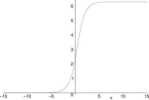
Figure 2.1: Single soliton solution

This configuration has two useful properties. First, it is a “soliton”, which means that it preserves its shape over time without dissipation or decay. Secondly, because it interpolates between vacua, it cannot be destroyed as that would alter the value of the field as $x\rightarrow\pm\infty$; for this reason, the theory is often called “topological”. The “topological charge” of a state is defined as the difference (in units of $\frac{2\pi}{\beta}$) between the value of the field at $-\infty$ and $+\infty$ and must be conserved. A single soliton state has charge 1, while an anti-soliton state (interpolating between the vacuum at $-\infty$ and the next lower one) has charge -1.

If two (anti-)solitons collide, they are simply transmitted through the collision, without changing shape, and so can truly be considered as particles (which, the theory being integrable, cannot be created or destroyed). If their rapidities are allowed to be complex, however, rather than purely real, the situation changes. If a soliton and an anti-soliton are given conjugate rapidities, a “bound state” appears. Due to the periodic up-and-down motion of the field, these particles are known as “breathers” and are categorised by the imaginary component of their rapidity, which determines their period and mass.

The soliton and anti-soliton both have the same mass, which we shall call $m_{s}$, while the mass of the breather formed by a soliton–anti-soliton pair at a relative rapidity of $\theta=iu$ is $m=2m_{s}\cos\left(\frac{u}{2}\right)$. That completes the particle spectrum of the bulk theory as, if two breathers are persuaded to bind together, they simply form a third breather.

2.5 Construction of boundary bound states

Rather than try to analyse the boundary theory in a similar way to the bulk, it is easier to use the method of images. The idea is to find a particular configuration of the bulk theory where the value of the field at $\varphi(0,t)$ happens to obey one of the integrable boundary conditions. The left-hand half line then provides a solution to the boundary theory.

The vacuum state of the boundary theory simply requires that $\varphi(0,t)=\varphi_{0}$ for all time, whatever the value of $M$, so a suitably-placed stationary soliton is all that is required. By analogy with electromagnetism, we might then imagine that the boundary state consisting of $n$ particles with rapidities $\theta_{1},\theta_{2},\ldots,\theta_{n}$ corresponds to the bulk state with an “image” set of particles behind the boundary (with opposite rapidities) and, again, a stationary soliton near the boundary.

This problem was first tackled by Saleur, Skorik and Warner [26], who found the 3-soliton solution. The choice as to whether each particle was a soliton or anti-soliton and their relative initial positions selected which boundary condition was obeyed. In addition, in the Neumann limit the position of the stationary particle became infinite, reducing the result to a two-soliton solution.

The natural generalisation of this is to consider a $2n+1$-soliton solution (which reduces to a $2n$-soliton solution in the Neumann limit). This is easier than it might appear as, in the limit where the particles are well separated (i.e. $t\rightarrow\pm\infty$), the state of the field at the boundary is determined only by the central stationary soliton and the two moving solitons that are closest, allowing the 3-soliton solution to be re-used.

In addition, as SSW found in the 3-soliton case, the absolute positions of each pair of moving solitons are irrelevant in the solution of the boundary condition; it is only the phase delay that is important. Using this fact, any pair of solitons in the $2n+1$-soliton solution can be moved off to infinity (provided their phase delay is preserved), reducing it to a $2n-1$-soliton solution. Using these two facts, it is perhaps beginning to become clear that the general solution can be built out of the 3-soliton solution with a little cunning.

2.5.1 Notation

For the classical problem, it is convenient to re-scale the field and coupling constant to re-express the bulk sine-Gordon equation as

$$\phi_{tt}-\phi_{xx}=-\sin(\phi)\,,$$ (2.19)

where $\beta\varphi\equiv\phi$. On the half line, the most general boundary condition then becomes

$$\partial_{x}\phi|_{x=0}=M\sin{\textstyle\frac{1}{2}}(\phi-\phi_{0})|_{x=0}\,.$$ (2.20)

The classical multi-soliton solution for the whole line has been known for some time, and is generally expressed in terms of Hirota’s $\tau$-functions [27] as

$$\phi(x,t)=4\arg(\tau)\equiv 4\arctan\left(\frac{\Im(\tau)}{\Re(\tau)}\right)\,,$$ (2.21)

where the $\tau$-function for an $N$-soliton solution is

$$\tau(x,t)=\sum_{\mu_{j}=0,1}\mathrm{e}^{\frac{i\pi}{2}\left(\sum_{j=1}^{N}\epsilon_{j}\mu_{j}\right)}\exp\left[-\sum_{j=1}^{N}{\textstyle\frac{1}{2}}\mu_{j}\left\{\left(k_{j}+\frac{1}{k_{j}}\right)x+\left(k_{j}-\frac{1}{k_{j}}\right)t-a_{j}\right\}\right.\\ \left.+2\sum_{1\leq i<j\leq N}\mu_{i}\mu_{j}\ln\left(\frac{k_{i}-k_{j}}{k_{i}+k_{j}}\right)\right]\,.$$ (2.22)

The parameters $k_{i}$ are related to the soliton rapidities by $k_{i}=\mathrm{e}^{\theta_{i}}$, so the solitons’ velocities are given by

$$v_{i}=\left(\frac{k_{i}^{2}-1}{k_{i}^{2}+1}\right)\,.$$ (2.23)

The $a_{i}$ represent the initial positions of the solitons (but see below) while the $\epsilon_{i}$ are +1(-1) for solitons (anti-solitons).

For the sake of simplicity, we shall number the particles in decreasing order of rapidity, so that particle 1 has the highest rapidity, particle 2 has the next highest, and so on. This ensures the logarithm in the $\tau$-function is always real. Other orderings give the same result—as they clearly must—but it is less transparent that the $\tau$-function is real.

2.5.2 The position problem

Before going any further, a problem immediately arises with the interpretation of the $a_{i}$ as the positions of the solitons. If this was truly the case, for example, a 3-soliton solution as $t\rightarrow\pm\infty$ would reduce to a single-soliton solution with the same value of the position parameter. This, however, is not true. The one-soliton solution is just

$$\tau_{1}(x,t)=1+i\epsilon_{1}\exp\left[-x+\frac{a_{1}}{2}\right]\,,$$ (2.24)

leading to

$$\phi_{1}(x,t)=4\arctan\left(\epsilon_{1}\exp\left[-x+\frac{a_{1}}{2}\right]\right)\,.$$ (2.25)

Taking the 3-soliton solution, note that, as $t\rightarrow\infty$, the soliton with positive rapidity will contribute a highly negative exponential whenever it appears in the sum, whereas the one with negative rapidity will contribute a correspondingly positive exponential. From this, it is clear that the two dominant terms will therefore be the ones where $\mu_{1}=0$ and $\mu_{3}=1$. Thus, as $t\rightarrow\infty$,

$$\tau_{3}(x,t) \approx \epsilon_{3}\exp\left[-\frac{1}{2}\left\{\left(k_{3}+\frac{1}{k_{3}}\right)x+\left(k_{3}-\frac{1}{k_{3}}\right)t-a^{\prime}_{3}\right\}\right]\cdot$$ (2.26)

$$\cdot\left(i-\epsilon_{2}\exp\left[-x+\frac{a^{\prime}_{2}}{2}+2\ln\left(\frac{1-k_{3}}{1+k_{3}}\right)\right]\right)\,,$$

leading to

$$\phi_{3}(x,t)\approx 4\arctan\left(-\epsilon_{2}\exp\left[x-\frac{a^{\prime}_{2}}{2}-2\ln\left(\frac{1-k_{3}}{1+k_{3}}\right)\right]\right)\,.$$ (2.27)

If we now remember that $\tan\left(x\pm\frac{\pi}{2}\right)=-\tan(x)^{-1}$, this implies that $4\arctan x=y$ can be re-written as $4\arctan-\frac{1}{x}=y\pm 2\pi$. Thus, we find

$$\phi_{3}(x,t)\pm 2\pi\approx 4\arctan\left(\epsilon_{1}\exp\left[-x+\frac{a^{\prime}_{2}}{2}+2\ln\left(\frac{1-k_{3}}{1+k_{3}}\right)\right]\right)\,.$$ (2.28)

The $2\pi$ on the lhs, which is equal to the spacing of the vacua, just represents the fact that the Hirota solution imposes $\phi=0$ at $-\infty$, while the natural assumption here is that $\phi=\pm 2\pi$, so that the leftmost soliton reduces the field to zero heading in towards the central particle. Thus, we do indeed have a single-soliton solution, but with

$$a_{1}=a^{\prime}_{2}+4\ln\left(\frac{1-k_{3}}{1+k_{3}}\right)\,.$$ (2.29)

Repeating this exercise with $t\rightarrow-\infty$ instead gives the same result, but with $k_{3}$ replaced by $\frac{1}{k_{1}}$. Since we would like the stationary soliton to solve the same boundary condition in both cases (as this condition stays unchanged for all time), it is clear that we are forced to take $k_{3}=\frac{1}{k_{1}}$, as SSW did.

The reason for this is easy to see once it is realised that, to shift the solution in time, all that is needed is to shift each position parameter by velocity$\times$time, irrespective of any collisions which may have happened in the interim. The effects of collisions are thus built into the solution, and the parameters are only indirectly related to particle positions at any given time. In what follows, however, it will be easier to work in terms of “actual” parameters, and transform back to Hirota’s parameters at the end.

A more general analysis shows that the $2N+1$-soliton solution with $N$ pairs of solitons with opposite rapidities examined at $t\rightarrow-\infty$ reduces to $2N+1$ single-soliton solutions as expected, but with each soliton position modified by a term involving all rapidities higher than its own. This means that the “position” parameters $a_{i}$ only have a genuine interpretation as a position for the particle with the highest rapidity. As $t\rightarrow+\infty$, the opposite situation arises, with the position parameters modified by all lower rapidities. To be precise, let us take $x\rightarrow+\infty$ and $t\rightarrow-\infty$ with $\frac{x}{t}\approx v_{i}$, to keep ourselves in the neighbourhood of particle $i$. This means that $i>N$ (we are considering the particles with negative rapidities). Then, by the same reasoning as before, the two dominant terms will be those with $\mu_{j}=1,j<i$ and $\mu_{j}=0,j>i$. This gives, for $i-1$ even,

$$\tau_{2N+1}(x,t)\approx(-1)^{\frac{i-1}{2}}\prod_{j=1}^{i-1}\epsilon_{j}\exp\left[-\sum_{j=1}^{i-1}\frac{1}{2}\left\{\left(k_{j}+\frac{1}{k_{j}}\right)x+\left(k_{j}-\frac{1}{k_{j}}\right)t-a_{j}\right\}\right.\\ \left.+2\sum_{1\leq i^{\prime}<j\leq i-1}\ln\left(\frac{k_{i^{\prime}}-k_{j}}{k_{i^{\prime}}+k_{j}}\right)\right]\times\\ \left(1+i\epsilon_{i}\exp\left[-\frac{1}{2}\left\{\left(k_{i}+\frac{1}{k_{i}}\right)x+\left(k_{i}-\frac{1}{k_{i}}\right)t-a_{i}\right\}\right.\right.\\ \left.\left.+2\sum_{1\leq j\leq i-1}\ln\left(\frac{k_{j}-k_{i}}{k_{i}+k_{j}}\right)\right]\right)\,,$$ (2.30)

leading to

$$\phi_{2N+1}(x,t)\approx 4\arctan\left(\epsilon_{i}\left[-{\textstyle\frac{1}{2}}\left\{\left(k_{i}+\frac{1}{k_{i}}\right)x+\left(k_{i}-\frac{1}{k_{i}}\right)t-a_{i}\right\}\right.\right.\\ \left.\left.+2\sum_{1\leq j\leq i-1}\ln\left(\frac{k_{j}-k_{i}}{k_{i}+k_{j}}\right)\right]\right)\,.$$ (2.31)

Thus, compared with the appropriate single soliton solution,

$$a_{1}=a_{i}+4\sum_{1\leq j\leq i-1}\ln\left(\frac{k_{j}-k_{i}}{k_{i}+k_{j}}\right)\,.$$ (2.32)

Note that, this time, $\phi\rightarrow 0$ as $x\rightarrow\infty$ is the natural situation, in agreement with the Hirota formula. For $2N+1-i$ odd, we need to use the same trick as for the three-soliton case, but finish up with the same formula. Finally, for $i\leq N$ we need to take $x\rightarrow-\infty$ but the result remains true. Taking the other limit (as $t\rightarrow+\infty$), the analogous result is

$$a_{1}=a_{i}+4\sum_{i+1\leq j\leq 2N+1}\ln\left(\frac{k_{i}-k_{j}}{k_{i}+k_{j}}\right)\,.$$ (2.33)

Note also that the only way to ensure the boundary condition stays constant in time is to impose $k_{i}=1/k_{2N+2-i}$.

From this, we can calculate the phase delay between any pair of particles with equal and opposite rapidities—$i$ and $2N+2-i$—in terms of their “actual” position parameters $a_{n}^{\prime}$ as $t\rightarrow-\infty$ as

$$a_{i}+a_{2N+2-i}=a^{\prime}_{i}+a^{\prime}_{2N+2-i}-4\sum_{j\neq i}\ln\left(\left|\frac{k_{j}-k_{i}}{k_{i}+k_{j}}\right|\right)\,,$$ (2.34)

assuming $i\leq N$.

2.5.3 Solving the boundary condition

As a warm up to the general solution, it is useful to consider the simplest possible solution, with only one stationary soliton. This corresponds to the ground state of the boundary model. In this case, all boundary conditions reduce to the demand that $\phi|_{x=0}=\Phi_{0}$, for some constant $\Phi_{0}$ depending on the boundary conditions. (In the Dirichlet case, $\Phi_{0}$ becomes simply $\phi_{0}$.) Putting this into (2.25), we find

$$\phi_{1}(0,t)=4\arctan\left(\epsilon_{1}\mathrm{e}^{\frac{a_{1}}{2}}\right)=\Phi_{0}\,,$$ (2.35)

implying

$$a_{1}=2\ln\left(\epsilon_{1}\tan\frac{\Phi_{0}}{4}\right)\,.$$ (2.36)

Taking advantage of the fact that the 3-soliton solution must tend to this near the origin as $t\rightarrow-\infty$, we can immediately write down the position parameter of the stationary soliton in the 3-soliton solution as

$$a_{2}=2\ln\left(\epsilon_{1}\tan\frac{\Phi_{0}}{4}\right)-4\ln\left(\frac{k_{1}-1}{k_{1}+1}\right)=2\ln\left(\epsilon_{1}\tan\frac{\Phi_{0}}{4}\left(\frac{k_{1}+1}{k_{1}-1}\right)^{2}\right)\,.$$ (2.37)

Noting that, in terms of the rapidity variable, $(\frac{k_{1}-1}{k_{1}+1})^{2}=\tanh\left(\frac{\theta}{2}\right)^{2}$, this agrees with the formula for $a_{3}$ given by SSW in their appendix. They derive this specifically for the case of Dirichlet boundary conditions, but it can now be seen to have the same form for all boundary conditions.

2.5.4 The general solution

By extension of the above argument, the position parameter of the stationary soliton in the $2N+1$-soliton solution is

$$a_{N+1}=2\ln\left(\epsilon_{N+1}\tan\frac{\Phi_{0}}{4}\prod_{1\leq j\leq N}\tanh\left(\frac{\theta_{j}}{-2}\right)^{2}\right)\,.$$ (2.38)

As has already been mentioned, the general $2N+1$-soliton solution reduces to the 3-soliton solution (involving the 3 slowest solitons) as $t\rightarrow-\infty$, so the phase delay for the slowest pair should be given by the SSW formula, which (with our conventions) is

$$a=2\ln\left\{-\epsilon_{1}\epsilon_{3}\tanh\left(\frac{\theta}{2}\right)^{-2}\tanh(\theta)^{-2}\left[\frac{\tanh{\textstyle\frac{1}{2}}(\theta+i\eta)\tanh{\textstyle\frac{1}{2}}(\theta-i\eta)}{\tanh{\textstyle\frac{1}{2}}(\theta+\zeta)\tanh{\textstyle\frac{1}{2}}(\theta-\zeta)}\right]^{\pm 1}\right\}\,,$$ (2.39)

where $\eta$ and $\zeta$ are the solutions of the simultaneous equations

$$M\cos({\textstyle\frac{1}{2}}\phi_{0}) = 2\cosh\zeta\cos\eta$$

$$M\sin({\textstyle\frac{1}{2}}\phi_{0}) = 2\sinh\zeta\sin\eta\,.$$ (2.40)

The ambiguity in the sign of (2.39) is simply a vagary of the solution method (due to the fact that the bulk vacua are $2\pi$-periodic, whereas the boundary vacua are only $4\pi$-periodic; working in terms of the bulk makes the stable and unstable possibilities appear together). We shall concentrate on the negative sign, which corresponds to the stable boundary value.

By virtue of (2.34), this can be re-written using the “actual” position parameters instead, as

$$a^{\prime}=2\ln\left\{-\epsilon_{1}\epsilon_{3}\left[\frac{\tanh{\textstyle\frac{1}{2}}(\theta+i\eta)\tanh{\textstyle\frac{1}{2}}(\theta-i\eta)}{\tanh{\textstyle\frac{1}{2}}(\theta+\zeta)\tanh{\textstyle\frac{1}{2}}(\theta-\zeta)}\right]^{\pm 1}\right\}\,.$$ (2.41)

Turning now to the faster particles, we need to use the fact that, for the slowest particles, only the phase delay is important. This means that we can take their actual positions off to $\pm\infty$ without affecting the validity of the solution, and essentially reduce the problem to the $2N-1$-soliton case. Now, the next slowest particles have gained the mantle of being the slowest, and so must have a phase delay of the same form. (Note that, in doing this, we have made the slowest particles collide with all the faster ones in turn on their way to infinity, changing their positions. The symmetry of the situation, however, ensures that the phase delays between the pairs of particles stay intact.)

Repeating this for all the particles shows that, for each pair, all that is relevant is the phase delay, and this always has the SSW form. In terms of the position parameters, we then have

$$a^{i}=2\ln\left\{-\epsilon_{i}\epsilon_{2N+2-i}\prod_{j\neq i}\tanh\left(\frac{\theta_{i}-\theta_{j}}{2}\right)^{-2}\left[\frac{\tanh{\textstyle\frac{1}{2}}(\theta+i\eta)\tanh{\textstyle\frac{1}{2}}(\theta-i\eta)}{\tanh{\textstyle\frac{1}{2}}(\theta+\zeta)\tanh{\textstyle\frac{1}{2}}(\theta-\zeta)}\right]^{\pm 1}\right\}\,,$$ (2.42)

where $a^{i}=a_{i}+a_{2N+2-i}$.

This completes the solution, but for one point: through this argument we have shown that if the $2N+1$-soliton solution exists then it must have the given form, but we have not shown that it actually exists. For that, we would need to substitute the results back into the Hirota formula to check—a cumbersome task, and one for which we lack the energy. In the meantime, we content ourselves with the observation that it seems a reasonable assumption, and bears up to all the numerical checks we have carried out.

2.6 Boundary bound states

2.6.1 Boundary breathers

The natural progression from this is to consider extending the rapidities to complex values. While this can be used give a solution where breathers rather than solitons interact with the boundary, it can also be used to construct “boundary breathers” or boundary bound states. These solutions arise when the pair of particles which are given complex conjugate rapidities consist of one in front of the boundary and one behind.

Due to the requirement that their rapidities must also be equal and opposite, this implies that they must be given purely imaginary rapidities. Curiously, in the Dirichlet case (as SSW noted) the pair of particles must also consist of two solitons or two anti-solitons, not a particle and its anti-particle as in the bulk.

Simply by continuing all rapidities to imaginary values, we can generate a sequence of bound states through solutions with successively greater numbers of solitons. The one subtlety is that both members of each pair have to be given the same initial position parameter for the solution to still obey the boundary condition. This is a consequence of the way the solution was found: the $\tau$-function was split into real and imaginary parts, assuming all rapidities were real. Making some rapidities imaginary disturbs this in general, but putting both members of each pair at the same position allows the split used to remain valid. Since all other solutions to the problem with real rapidities can be related to this by a time translation, it is reasonable to assume that the same is true for the imaginary case. The only difference is that, with imaginary rapidities, there is no movement in real space.

As with the bulk breathers, the period of a boundary breather is given through the imaginary part of the rapidity. For the 3-soliton solution, with the moving pair given a rapidity of $\theta=iu$, the period is $2\pi/\sin(u)$. Now, however, for the breathers coming from higher solutions, each pair has its own period. If there exists a common period, whose length is an integer multiple of the periods of all the pairs, then the motion is still periodic, but, in general, it will now be aperiodic.

To demonstrate the form of the boundary breathers, we have chosen periodic solutions by giving each pair an integer period. These are shown in Figures 2.2, 2.3, and 2.4 for the 3, 5, and 7 soliton solutions respectively.

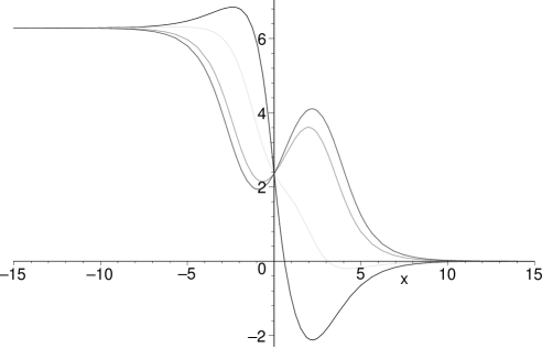
Figure 2.2: 3-soliton solution, period 10

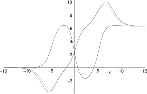
Figure 2.3: 5-soliton solution, periods 10 and 12

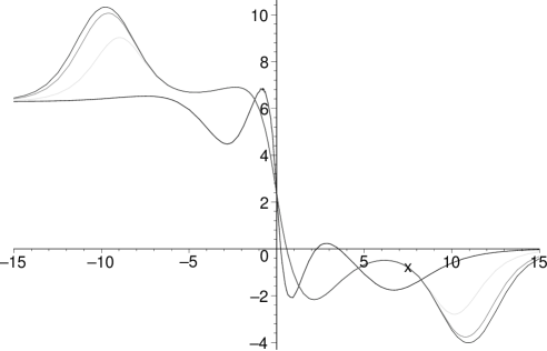
Figure 2.4: 7-soliton solution, periods 10, 12, and 14

2.6.2 Another bound state

The breathers mentioned above are not the only bound states in the classical theory. The phase delay (2.41) becomes infinite at $\theta=\zeta$, which must be due to the formation of a stable bound state. In the bulk theory, this could not happen (all bound states must be formed at imaginary rapidities), so it is further evidence of the changes wrought by the introduction of a boundary.

Considering the 3-soliton solution, we can imagine the particle with negative rapidity as being taken off to infinity at this point, leaving just a two-particle process. The remaining moving particle sweeps past the boundary, shifting the stationary soliton on the way past; this only appears as a bound state when we restrict ourselves to the half line. Then, the incoming particle reaches the boundary and disappears, leaving the boundary state changed.

The final state can be found by considering the limit of the 3-particle $\tau$-function where the position parameters of both moving particles are taken to infinity. The result of this is that $\phi_{0}$ becomes $\phi^{\prime}_{0}$, given by

$$\tan\left(\frac{\phi^{\prime}_{0}}{4}\right)=\tan\left(\frac{\phi_{0}}{4}\right)\tanh^{4}\left(\frac{\zeta}{2}\right)\,.$$ (2.43)

2.7 Predictions

The first prediction to take across to the discussion of the quantum theory is that there should be a hierarchy of excited states. For example, the states formed by binding a soliton to the boundary should be analogous to the 3-soliton solution found above. After that, further solitons should create the quantum versions of $5,7,\ldots$ soliton solutions. Furthermore, the introduction of a breather should allow the formation of a state which could otherwise have been formed by two successive solitonic particles.

A final, and slightly more subtle point, is that the “actual” position parameter used for a given pair of particles (with imaginary rapidity) is monotonically decreasing for $u<\eta$, as shown in figure 2.5. This means that, in a given solution, the soliton pair with the least rapidity will be positioned farthest from the boundary. If we imagine that such a solution, translated into the quantum regime, is built up with the soliton finally positioned nearest the boundary interacting first, this means that particles must interact in decreasing order of rapidity.

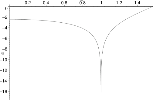
Figure 2.5: Plot of $\mathbf{a^{\prime}}$ versus $\mathbf{u}$ for $\mathbf{\eta=1.0}$

Chapter 3 Quantum Boundary sine-Gordon Theory

“The most exciting phrase to hear in science, the one that heralds new discoveries, is not ‘Eureka!’ but ‘That’s funny…”’

—Isaac Asimov

3.1 Introduction

“Mathematicians are a species of Frenchman: if you say something to them they translate it into their own language and presto! it is something entirely different.”

—Goethe

As we saw in the previous chapter, introducing a boundary into the classical theory brings with it a number of new phenomena, and in particular a new set of boundary bound states. In this chapter, we will investigate these further in the full quantum sine-Gordon model.

A major complicating factor in this work is the fact that even simple poles in the boundary reflection factors should not necessarily be interpreted as being due to the formation of bound states, since many have an interpretation through the Coleman-Thun mechanism. Indeed, this model provides a good arena for demonstrating the range of possible explanations this mechanism can throw up, in some cases involving bulk and boundary matrices working together to induce a cancellation in the naïve order of a diagram.

The two main tasks, therefore, are to find suitable interpretations where required, but also to find a method of proving that the remaining poles are indeed associated with bound states. Two elementary lemmas—which simply serve to impose momentum conservation on boundary processes—will turn out to give us all the ammunition we need for this, and should also be readily applicable to other models.

The groundwork for the study of the boundary sine-Gordon model was laid by Ghoshal and Zamolodchikov [13], before being taken further by Ghoshal [28] and Skorik and Saleur [29]. They provided the basic ground-state reflection factors, and investigated the first few excited states; we will take this forward to provide (hopefully) a full and rigorous solution to the problem.

After reviewing these results in the first section, we will go on to a detailed investigation of the Dirichlet boundary condition (where the value of the field at the boundary is fixed for all time). This displays most of the features of the general solution, and will allow us to extend the results straightforwardly to all other integrable boundary conditions.

3.2 Review of previous results

3.2.1 The theory in the bulk

As we discussed in the previous chapter, the classical sine-Gordon model (2.1) is integrable. This can be shown to be true at the quantum level as well [30] and so the exact quantum S-matrix can be found through the axiomatic program. The essential difference between the classical and quantum theories is that the breather particles, which could be formed classically by a soliton–anti-soliton pair at any imaginary rapidity, now become quantised. These states can now only be formed at relative rapidities of $i\left(\pi-n\pi/2\lambda\right)$, $n=1,2,\ldots,<\lambda$, where

$$\lambda=\frac{8\pi}{\beta^{2}}-1\,,$$ (3.1)

and so will be labelled as $B_{n}$. Their mass is therefore $m_{n}=2m_{s}\sin\left(n\pi/2\lambda\right)$.

If we denote the soliton S-matrix as $S^{ab}_{cd}(\theta)$ for rapidity $\theta$, with $a,b,c,d$ taking the value $+$ ($-$) if the particle is a soliton (anti-soliton), the non-zero scattering amplitudes [11] are $S^{++}_{++}(\theta)=S^{--}_{--}(\theta)=a(\theta)$ (soliton-soliton or anti-soliton-anti-soliton scattering), $S^{+-}_{+-}(\theta)=S^{-+}_{-+}(\theta)=b(\theta)$ (soliton-anti-soliton transmission), and $S^{+-}_{-+}(\theta)=S^{-+}_{+-}(\theta)=c(\theta)$ (soliton-anti-soliton reflection). Explicitly,

$$a(\theta) = \sin[\lambda(\pi-u)]\rho(u)\,,$$

$$b(\theta) = \sin(\lambda u)\rho(u)\,,$$ (3.2)

$$c(\theta) = \sin(\lambda\pi)\rho(u)\,,$$

where $u=-i\theta$ and

$$\rho(u)=\frac{1}{\sin(\lambda(u-\pi))}\prod_{l=1}^{\infty}\left[\frac{\Gamma\left((2l-2)\lambda-\frac{\lambda u}{\pi}\right)\Gamma\left(1+2l\lambda-\frac{\lambda u}{\pi}\right)}{\Gamma\left((2l-1)\lambda-\frac{\lambda u}{\pi}\right)\Gamma\left(1+(2l-1)\lambda-\frac{\lambda u}{\pi}\right)}/(u\rightarrow-u)\right].$$ (3.3)

As pointed out in [31], this factor can also be written in terms of Barnes’ diperiodic sine function $S_{2}(x|\omega_{1},\omega_{2})$ [32, 33]. This is a meromorphic function parametrised by the pair of ‘quasiperiods’ $(\omega_{1},\omega_{2})$, with poles and zeroes at the following points:

poles $$: x=n_{1}\,\omega_{1}+n_{2}\,\omega_{2}~{}~{}~{}~{}(n_{1},n_{2}=1,2,\dots)$$

zeroes $$: x=m_{1}\,\omega_{1}+m_{2}\,\omega_{2}~{}~{}~{}(m_{1},m_{2}=0,-1,-2\dots)$$ (3.4)

In terms of this function,

$$\rho(u)=\frac{1}{\sin(\lambda(u-\pi))}\frac{S_{2}\left(\pi-u\left|\frac{\pi}{\lambda},2\pi\right.\right)S_{2}\left(u\left|\frac{\pi}{\lambda},2\pi\right.\right)}{S_{2}\left(\pi+u\left|\frac{\pi}{\lambda},2\pi\right.\right)S_{2}\left(-u\left|\frac{\pi}{\lambda},2\pi\right.\right)}\,.$$ (3.5)

The amplitudes $b(\theta)$ and $c(\theta)$ have simple poles at $\theta=i\left(\pi-\frac{n\pi}{\lambda}\right)$, $n=1,2,\ldots,<\lambda$, which can be attributed to the creation of $B_{n}$ in the forward channel. There are also poles at $\theta=\frac{i\pi n}{\lambda}$ in $a(\theta)$ and $b(\theta)$ corresponding to the same process in the cross channel. Since all poles that we will be discussing, both in the bulk and at the boundary, occur at purely imaginary rapidities, from now on we will use the variable $u=-i\theta$ and always work in terms of purely imaginary rapidities.

3.2.2 The theory with a boundary

Returning again to the previous chapter, the bulk theory be restricted to the half-line $x\in(-\infty,0]$ while still preserving integrability by adding a “boundary action” term [13]

$$-\int_{-\infty}^{\infty}dt\,M\cos\left[\frac{\beta}{2}(\varphi^{\phantom{1}}_{B}-\varphi^{\phantom{1}}_{0})\right],$$ (3.6)

where $M$ and $\varphi_{0}$ are free parameters, and $\varphi^{\phantom{1}}_{B}(t)=\varphi(x,t)|_{x{=}0}$.

This does not conserve topological charge in general, so four solitonic boundary reflection factors need to be introduced, as well as a set of breather reflection factors. The solitonic factors which we quote here were given in [13], while breather factors can be found in [28].

Solitonic ground state factors

The reflection factors for the sine-Gordon solitons off the boundary ground state will be denoted by $P_{\pm}(u)$ (a soliton or anti-soliton, incident on the boundary, is reflected back unchanged) and $Q_{\pm}(u)$ (a soliton is reflected back as an anti-soliton, or vice versa). These are given by

$$\begin{array}[]{rcl}P^{+}(u)&=&\cos(\xi+\lambda u)R(u)\\ P^{-}(u)&=&\cos(\xi-\lambda u)R(u)\\ Q^{\pm}(u)&=&\frac{k}{2}\sin(2\lambda u)R(u),\end{array}$$ (3.7)

where

$$R(u)=R_{0}(u)R_{1}(u).$$ (3.8)

The first factor—$R_{0}(u)$—is boundary-independent, and can be written as

$$R_{0}(u)=\prod_{k=1}^{\infty}\left[\frac{\Gamma\left(1+\lambda(4k-4)-\frac{2\lambda u}{\pi}\right)\Gamma\left(4\lambda k-\frac{2\lambda u}{\pi}\right)}{\Gamma\left(\lambda(4k-3)-\frac{2\lambda u}{\pi}\right)\Gamma\left(1+\lambda(4k-1)-\frac{2\lambda u}{\pi}\right)}/(u\rightarrow-u)\right]\,.$$ (3.9)

The boundary-dependent term is $R_{1}(u)$, given by

$$R_{1}(u)=\frac{1}{\cos\xi}\sigma(\eta,u)\sigma(i\vartheta,u),$$ (3.10)

where

$$\sigma(x,u)=\frac{\Pi\left(x,\frac{\pi}{2}-u\right)\Pi\left(-x,\frac{\pi}{2}-u\right)\Pi\left(x,-\frac{\pi}{2}+u\right)\Pi\left(-x,-\frac{\pi}{2}+u\right)}{\Pi\left(x,\frac{\pi}{2}\right)\Pi\left(x,-\frac{\pi}{2}\right)\Pi\left(-x,\frac{\pi}{2}\right)\Pi\left(-x,-\frac{\pi}{2}\right)},$$ (3.11)

and

$$\Pi(x,u)=\prod_{l=0}^{\infty}\frac{\Gamma\left(\frac{1}{2}+\left(2l+\frac{1}{2}\right)\lambda+\frac{x}{\pi}-\frac{\lambda u}{\pi}\right)\Gamma\left(\frac{1}{2}+\left(2l+\frac{3}{2}\right)\lambda+\frac{x}{\pi}\right)}{\Gamma\left(\frac{1}{2}+\left(2l+\frac{3}{2}\right)\lambda+\frac{x}{\pi}-\frac{\lambda u}{\pi}\right)\Gamma\left(\frac{1}{2}+\left(2l+\frac{1}{2}\right)\lambda+\frac{x}{\pi}\right)}.$$ (3.12)

The parameters $\xi,\eta,\vartheta,$ and $k$ are real and arbitrary apart from being constrained by

$$\begin{array}[]{rcl}\cos(\eta)\cosh(\vartheta)&=&-\frac{1}{k}\cos\xi\\ \cos^{2}(\eta)+\cosh^{2}(\vartheta)&=&1+\frac{1}{k^{2}}.\end{array}$$ (3.13)

The relationship of these parameters—which arise in the course of finding the most general solution to the four requirements given in Chapter 1—to the ones which appear in the action was, for a long time, unknown. The problem has only recently been solved by Al. Zamolodchikov; further details can be found in Appendix A.2. These formal parameters, however, are easier to work with in practice than the physical $\varphi_{0}$ and $M$, and so we shall continue to use them.

The theory is invariant under $\varphi_{0}\to\varphi_{0}+\frac{2\pi}{\beta}$, and also under the simultaneous transformations $\varphi_{0}\rightarrow-\varphi_{0}$ and $\mathrm{soliton\ }\rightarrow\mathrm{anti{-}soliton}$. Introducing the boundary breaks the degeneracy of the bulk vacua, and selects the lower line in figure 3.1 as the lowest-energy state, with the upper line as the first excited state. Continuing $\varphi_{0}$ through $\frac{\pi}{\beta}$ thus simply interchanges the rôles of these two states, and selects the upper one as the ground state.

Figure 3.1: Vacuum structure

In light of this, we are free to choose $\varphi_{0}$ to be in the interval $0<\varphi_{0}<\frac{\pi}{\beta}$. Note also that the topological charge of the ground state is no longer zero, as in the bulk model, but

$$q=\frac{\beta}{2\pi}\int_{-\infty}^{0}dx\frac{\partial}{\partial x}\varphi(x,t)=\frac{\beta}{2\pi}[\varphi(0,t)-\varphi(-\infty,t)]=\frac{\beta\varphi_{0}}{2\pi}\,,$$ (3.14)

with the charge of the first excited state being $1-\frac{\beta\varphi_{0}}{2\pi}$. We will find—at least for the Dirichlet case—that all the boundary states have one of these charges so, for convenience, we shall designate them simply as 0 and 1 respectively.

Breather ground state reflection factors

For the breather sector, Ghoshal [28] obtained the relevant reflection factors—$R^{n}_{|0\rangle}(u)$ for breather $n$ and boundary ground state $|0\rangle$—from the solitonic reflection factors using the general boundary bootstrap equation [20, 13]

$$f^{n}_{i_{1}i_{2}}R^{i_{1}}_{j_{1}|x\rangle}\left(u+\frac{u_{n}}{2}\right)S_{j_{2}f_{1}}^{i_{2}j_{1}}(2u)R^{j_{2}}_{f_{2}|x\rangle}\left(u-\frac{u_{n}}{2}\right)=f^{n}_{f_{1}f_{2}}R^{n}_{|x\rangle}(u),$$ (3.15)

where $u_{n}=\pi-\frac{n\pi}{\lambda}$, and the $R^{a}_{b|x\rangle}(u)$ are the solitonic reflection factors, such that $R^{+}_{-|x\rangle}(u)$ is the factor for a soliton to be reflected back as an anti-soliton and so on. The $f^{n}_{ab}$ are the bulk vertices for the creation of breather $n$ from (anti-)solitons $a$ and $b$. These obey $f^{n}_{+-}=(-1)^{n}f^{n}_{-+}$. The bootstrap is illustrated in figure 3.2.

=  

Figure 3.2: Breather bootstrap

3.3 The boundary Coleman-Thun mechanism

To discover the boundary spectrum, the most natural approach is to look for simple poles in the reflection factors, which might be expected to be related to the formation of boundary bound states. As we have already mentioned in section 1.2.4, however, a complicating factor is the fact that not all simple poles correspond to bound states, some having an interpretation as anomalous threshold singularities.

This problem becomes especially serious once a boundary is involved, due to the increased complexity of the on-shell diagrams which become possible. This makes it hard to be sure that any given pole really does correspond to a new boundary bound state. In the bulk, a simple geometrical argument shows that poles in the S-matrix elements of the lightest particle can never be explained by a Coleman-Thun mechanism, and so must always be due to bound states [17]. We wish to find analogous criteria for the boundary situation. To this end, the following two lemmas turn out to be useful. Suppose the incoming particle is of type $a$, and that its reflection factor has a simple pole at $\theta=iu$.

Lemma 1

Let $\overline{U}_{a}=\min_{b,c}\left(\pi-U^{c}_{ab}\right)$. If $u<\overline{U}_{a}$, then the the pole at $iu$ cannot be explained by a Coleman-Thun mechanism, and so must correspond to the binding of particle $a$ to the boundary, either before or after crossing the outgoing particle.

Proof: All processes must take the form shown in figure 3.4 or the crossed version shown in figure 3.4. Conservation of momentum demands that all rescattering must take place within the hatched region, which is drawn from the furthest point from the boundary where either the incoming or outgoing particle undergoes any interaction. If neither particle decays, we simply have a diagram of the form of figure 3.9 or figure 3.9. Otherwise, momentum conservation requires that neither product of the particle which decays on the boundary of the hatched region has a trajectory which takes it outside that region. Fixing the notation by figure 3.6 (with angles $U^{b}_{ac}$ and $U^{c}_{ab}$ defined correspondingly), this reduces to demanding $\pi-U^{c}_{ab}\leq u\leq U^{b}_{ac}$. If we introduce $\overline{U}_{a}$ then we must have $\overline{U}_{a}\leq u\leq\pi-\overline{U}_{a}$ (i.e. just $u\geq\overline{U}_{a}$, as $u\leq\frac{\pi}{2}$). Thus, if $u<\overline{U}_{a}$, then the only possible explanations for the pole are figure 3.9 and figure 3.9.

Lemma 2

If the boundary is in its ground state, then lemma 1 can be strengthened, requiring that the incoming particle bind to the boundary if $u$ is outside the range $\overline{U}_{a}<u<\frac{\pi}{2}-\overline{U}_{a}$. In addition, if $\min_{b,c}U^{a}_{bc}>\frac{\pi}{2}$, the incoming particle must always bind to the boundary.

Proof: With the boundary in its ground state, all rescattering must take place in the area shown in figure 3.6. Reasoning as before but demanding that both product particles be emitted into this more restricted region, we find $\pi-U^{c}_{ab}\leq u\leq U^{b}_{ac}-\frac{\pi}{2}$, or $\overline{U}_{a}\leq u\leq\frac{\pi}{2}-\overline{U}_{a}$. In addition, both particles $b,c$ must be emitted into an angle of $\frac{\pi}{2}$, so $U^{a}_{bc}<\frac{\pi}{2}$ for at least one pair of particles $b$, $c$. If either of these conditions are violated, then the incoming particle must bind to the boundary.

Figure 3.3: General process, with incoming particles uncrossed

Figure 3.4: General process, with incoming particles crossed

Figure 3.5: General process when boundary is in ground state

Figure 3.6: Decay process

These two results, between them, will allow the spectrum of the boundary sine-Gordon model to be fixed completely, provided it is assumed that no pole corresponds to the creation of a boundary state if it has an alternative (Coleman-Thun) explanation.

For the problem under discussion, writing the rapidity bounds $\overline{U}_{a}$ as $\overline{U}_{+(-)}$ for the soliton (anti-soliton) and as $\overline{U}_{n}$ for the $B_{n}$, we have

$$\overline{U}_{\pm} = \frac{\pi}{2}-\frac{n_{\mathrm{max}}\pi}{2\lambda}$$

$$\overline{U}_{n} = \frac{\pi}{2\lambda}~{},~{}~{}~{}n\neq n_{max}$$ (3.16)

$$\overline{U}_{n_{\mathrm{max}}} = \frac{\pi}{2}-\frac{n_{\mathrm{max}}\pi}{2\lambda}\,,$$

where $B_{n_{max}}$ is the highest-numbered breather present in the model. To derive these results, note that a soliton (anti-soliton) can only decay into an anti-soliton (soliton) and a breather (with vertex $U^{\pm}_{\mp n}=\frac{\pi}{2}+\frac{n\pi}{2\lambda}$). A breather can either decay into a soliton–anti-soliton pair ($U^{n}_{+-}=\pi-\frac{n\pi}{\lambda}$) or a pair of breathers ($U^{l}_{nm}=\pi-\frac{l\pi}{2\lambda}$ with $n=m+l$ or $m=n+l$, or $U^{l}_{nm}=\frac{\pi(n+m)}{2\lambda}$ with $l=n+m$).

These restrictions can also be combined to produce a stronger version of lemma 1 when the incoming particle is a soliton. If $\overline{U}_{+}<u<\frac{\pi}{\lambda}$, decay within the hatched region is only possible into the topmost breather and an anti-soliton. One or other of these particles will be heading away from the centre of the diagram. If the process in uncrossed, as in figure 3.4, the breather will be created heading towards the centre of the diagram, the anti-soliton away (we are being somewhat cavalier with the direction of time; this should be considered as a purely geometric argument). The anti-soliton must itself obey our lemmas; if in any further decay before it reaches the boundary one of the decay products is heading away from the boundary, then there would be no way to close the diagram while conserving momentum at every vertex. For a crossed process (figure 3.4) the breather is the outermost particle, and is again restricted in its decay by our lemmas for the same reason.

The anti-soliton created by the uncrossed process heads for the boundary with a rapidity less than $\overline{U}_{-}$ and so, by lemma 1, may not decay. By the same token, the breather of the crossed process cannot decay either so, if the initial soliton is not to form a bound state, the only possible alternative processes are figure A.2 and figure A.4. If these are found not to occur (for example, if the necessary boundary vertices are not present) then the pole must correspond to a bound state for any $u<\frac{\pi}{\lambda}$.

3.4 The Dirichlet case

3.4.1 The soliton sector

The Dirichlet case is exceptional in that topological charge is conserved and so $Q_{\pm}=0$. The remaining factors can be rewritten as

$$P^{\pm}(u)=R_{0}(u)\prod_{l=1}^{\infty}\left[\frac{\Gamma\left(\frac{1}{2}+2l\lambda\pm\frac{\xi}{\pi}+\frac{\lambda u}{\pi}\right)\Gamma\left(\frac{1}{2}+(2l-2)\lambda\mp\frac{\xi}{\pi}+\frac{\lambda u}{\pi}\right)}{\Gamma\left(\frac{1}{2}+(2l-1)\lambda+\frac{\xi}{\pi}+\frac{\lambda u}{\pi}\right)\Gamma\left(\frac{1}{2}+(2l-1)\lambda-\frac{\xi}{\pi}+\frac{\lambda u}{\pi}\right)}/\right.\\ \left.(u\rightarrow-u)\right]\,,$$ (3.17)

where $R_{0}(u)$ is as before and $\xi=\eta=\frac{4\pi\varphi_{0}}{\beta}$. Taking $\varphi_{0}$ to lie in $0<\varphi_{0}<\frac{\pi}{\beta}$, $\xi$ is in the range

$$0<\xi<\frac{\pi(\lambda+1)}{2}\,.$$ (3.18)

These factors can again be written in terms of Barnes’ multiperiodic functions, as

$$P^{\pm}(u)=R_{0}(u)\frac{S_{2}\left(\frac{\pi}{2\lambda}\mp\frac{\xi}{\lambda}+\pi+u\left|\frac{\pi}{\lambda},2\pi\right.\right)S_{2}\left(\frac{\pi}{2\lambda}\mp\frac{\xi}{\lambda}-u\left|\frac{\pi}{\lambda},2\pi\right.\right)}{S_{2}\left(\frac{\pi}{2\lambda}\mp\frac{\xi}{\lambda}+\pi-u\left|\frac{\pi}{\lambda},2\pi\right.\right)S_{2}\left(\frac{\pi}{2\lambda}\mp\frac{\xi}{\lambda}+u\left|\frac{\pi}{\lambda},2\pi\right.\right)},$$ (3.19)

with

$$R_{0}(u)=\frac{S_{2}\left(\frac{\pi}{2}-u\left|\frac{\pi}{2\lambda},2\pi\right.\right)S_{2}\left(\frac{\pi}{2\lambda}+u\left|\frac{\pi}{2\lambda},2\pi\right.\right)}{S_{2}\left(\frac{\pi}{2}+u\left|\frac{\pi}{2\lambda},2\pi\right.\right)S_{2}\left(\frac{\pi}{2\lambda}-u\left|\frac{\pi}{2\lambda},2\pi\right.\right)}.$$ (3.20)

3.4.2 The breather sector

In the Dirichlet case, with topological charge conserved, the bootstrap equation reduces to

$$f^{n}_{i_{1}i_{2}}P^{i_{1}}_{|x\rangle}\left(u+\frac{u_{n}}{2}\right)S^{i_{2}i_{1}}_{f_{2}f_{1}}(2u)P^{f_{2}}_{|x\rangle}\left(u-\frac{u_{n}}{2}\right)=f^{n}_{f_{1}f_{2}}R^{n}_{|x\rangle}(u).$$ (3.21)

Ghoshal found that, for the boundary ground state, the breather reflection factors were

$$R^{n}_{|0\rangle}(u)=R^{(n)}_{0}(u)R^{(n)}_{1}(u),$$ (3.22)

where

$$R_{0}^{(n)}(u)=\frac{\left(\frac{1}{2}\right)\left(\frac{n}{2\lambda}+1\right)}{\left(\frac{n}{2\lambda}+\frac{3}{2}\right)}\prod_{l=1}^{n-1}\frac{\left(\frac{l}{2\lambda}\right)\left(\frac{l}{2\lambda}+1\right)}{\left(\frac{l}{2\lambda}+\frac{3}{2}\right)^{2}},$$ (3.23)

and

$$R_{1}^{(n)}(u)=\prod_{l=\frac{1-n}{2}}^{\frac{n-1}{2}}\frac{\left(\frac{\xi}{\lambda\pi}-\frac{1}{2}+\frac{l}{2\lambda}\right)}{\left(\frac{\xi}{\lambda\pi}+\frac{1}{2}+\frac{l}{2\lambda}\right)}.$$ (3.24)

This makes use of the notation

$$(x)=\frac{\sinh\left(\frac{\theta}{2}+\frac{i\pi x}{2}\right)}{\sinh\left(\frac{\theta}{2}-\frac{i\pi x}{2}\right)},$$ (3.25)

which will also be helpful later.

3.5 Initial pole analysis

3.5.1 Solitonic ground state factors

The $R_{0}(u)$ factor is insensitive to the boundary parameters, and so all its poles should be explicable in terms of the bulk. The only poles are at $u=\frac{N\pi}{2\lambda}$, where $N=1,2,3,\ldots$, with no zeroes. These can be explained by the creation of a breather which is incident perpendicularly on the boundary, as shown in figure 3.9. Here, as in all subsequent diagrams, the time axis points up the page, and the $x$ axis points to the right. Solitons and anti-solitons are drawn as solid lines, while breathers are drawn as dotted lines.

Figure 3.7: poles
$\mathbf{\xi}$-independent pole

Figure 3.8: Bound
Bound state

Figure 3.9: Crossed
Crossed process

Turning now to $\xi$-dependent poles and zeroes, we find zeroes at

$$u=-\frac{\xi}{\lambda}+\frac{(2n+1)\pi}{2\lambda},$$ (3.26)

where $n=0,1,2,\ldots$, for $P^{+}$, and at the same rapidities but with $\xi\rightarrow-\xi$ for $P^{-}$. There are also poles in $P^{+}$ only at $u=\nu_{n}$, with

 $$\nu_{n}=\frac{\xi}{\lambda}-\frac{(2n+1)\pi}{2\lambda_{\phantom{l}}}$$  (3.27)

A soliton can only decay into an anti-soliton and a breather, with a rapidity difference between the two of $\frac{\pi}{2}+\frac{b\pi}{2\lambda}$ for breather $b$. Thus, by lemma 2, all these poles must correspond to bound states, as shown in figure 3.9. For reasons which will become clear in a moment, we shall depart from the convention of [29] and, rather than labelling the state corresponding to pole $\nu_{n}$ as $\beta_{n}$, will label it according to topological charge and $n$ as $|1;n\rangle$.

3.5.2 Solitonic excited state reflection factors

Using the boundary bootstrap equations given in [13]—which come from considering figure 3.10—solitonic reflection factors can be calculated for this first set of bound states. In our case, these equations read

$$P^{b}_{|y\rangle}(u)=\sum_{c,d}P^{d}_{|x\rangle}(u)S^{ab}_{cd}(u-\alpha_{ax}^{y})S^{dc}_{ba}(u+\alpha_{ax}^{y}),$$ (3.28)

where $a,b,c$, and $d$ take the values $+$ or $-$ and $\alpha_{ax}^{y}$ is the (imaginary) rapidity of the pole at which particle $a$ binds to boundary state $|x\rangle$ to give state $|y\rangle$. The mass of state $|y\rangle$—$m_{y}$—is given by

$$m_{y}=m_{x}+m_{s}\cos\alpha_{ax}^{y}\,.$$ (3.29)

=  

Figure 3.10: Boundary bound-state bootstrap

Taking $x$ to be the ground state $|0\rangle$ and $y$ to be one of the set of excited states $|1;n\rangle$, this gives

$$P^{+}_{|1;n\rangle}(u) = P^{+}_{|0\rangle}(u)a(u-\nu_{n})a(u+\nu_{n})$$

$$P^{-}_{|1;n\rangle}(u) = P^{-}_{|0\rangle}(u)b(u-\nu_{n})b(u+\nu_{n})+P^{+}_{|0\rangle}(u)c(u-\nu_{n})c(u+\nu_{n}).$$ (3.30)

Note that $P^{\pm}_{|1;0\rangle}(u)=\overline{P^{\mp}_{|0\rangle}(u)}$, where $\overline{P^{\pm}(u)}$ is $P^{\pm}(u)$ under the transformation $\xi\rightarrow\pi(\lambda+1)-\xi$. The reason for this is clear if we look back at figure 3.1; this transformation is equivalent to reflecting the diagram in the horizontal axis, interchanging the ground and first excited states.

Perhaps the neatest way to write the new reflection factors is

$$P^{\pm}_{|1;n\rangle}(u)=\overline{P^{\mp}(u)}a^{1}_{n}(u),$$ (3.31)

where

$$a^{1}_{n}(u)=\frac{a(u+\nu_{n})a(u-\nu_{n})}{a(u+\nu_{0})a(u-\nu_{0})}.$$ (3.32)

The factor $a^{1}_{n}(u)$ simplifies to

$$a^{1}_{n}(u)=\prod_{x=1}^{n}\frac{\left(\frac{\xi}{\lambda\pi}+\frac{1}{2\lambda}-\frac{x}{\lambda}\right)\left(\frac{\xi}{\lambda\pi}-\frac{1}{2\lambda}-\frac{x}{\lambda}\right)}{\left(\frac{\xi}{\lambda\pi}+\frac{1}{2\lambda}-\frac{x}{\lambda}+1\right)\left(\frac{\xi}{\lambda\pi}-\frac{1}{2\lambda}-\frac{x}{\lambda}+1\right)}.$$ (3.33)

Looking at the pole structure, we find that the functions $\overline{P^{\pm}(u)}$ have common simple poles at $\nu_{0}$ and $\nu_{-N}$ where $N=1,2,3,\ldots$ . In addition, $\overline{P^{+}(u)}$ has simple poles at $u=w_{N^{\prime}}$, where

 $$w_{N^{\prime}}=\pi-\frac{\xi}{\lambda}-\frac{\pi(2N^{\prime}-1)}{2\lambda_{\phantom{l}}}=\overline{\nu_{N^{\prime}}}$$  (3.34)

and $N^{\prime}=1,2,3,\ldots$, and simple zeroes at $-w_{N^{\prime\prime}}$ for appropriate values of $N^{\prime\prime}$. Finally, $a^{1}_{n}(u)$ has simple poles at $\nu_{0}$ and $\nu_{n}$, and double poles at $\nu_{k}$, $k=1,2,\ldots,n-1$.

Before proceeding to a more rigorous discussion, we shall now digress to give an outline of how the bootstrap might be expected to work. If one of these poles does correspond to a new bound state, factorisability leads us to expect that moving the soliton and anti-soliton trajectories past each other (so that the anti-soliton is incident on the boundary first) should also create the same state. The most obvious explanation for this would be for the anti-soliton to bind to the boundary first, followed by the soliton, to form the state. From above, however, only solitons can bind to the ground state, so we must look further.

The next most obvious way this could happen is via the soliton and anti-soliton forming a breather, either before or after the anti-soliton has reflected from the boundary. The poles required to allow the first process (of the form $\pi+\frac{\xi}{\lambda}-\frac{\pi(2m+1)}{2\lambda}$) are not present, whereas those necessary for the second (of the form $w_{m}$) are. Our candidate process therefore becomes figure 3.11, where the soliton and anti-soliton bind to form a breather, which then creates the state in one step. It is quite difficult to imagine any further alternatives, so let us—for the moment—take the existence of such a process as a necessary condition for a pole to be responsible for the formation of a boundary state.

=  

Figure 3.11: States can be created either by breathers or solitons

The consequence of this is that the $w_{N}$ poles are selected as the only possible candidates, and it appears that new bound states can only be formed by anti-solitons. Such states hence have charge 0 (agreeing with the idea that they can also be formed from the ground state by the action of a breather). In addition, it is also clear that only those $w_{N}$ such that $w_{N}<\nu_{n}$ can be considered, as, otherwise, the breather version of the process would see the breather created heading away from the boundary, rather than towards it.

Designating such a new state as $|0;n,N\rangle$ and bootstrapping on it leads to

$$P^{-}_{|0;n,N\rangle}(u) = P^{-}_{|1;n\rangle}(u)a(u-w_{N})a(u+w_{N})$$ (3.35)

$$P^{+}_{|0;n,N\rangle}(u) = P^{+}_{|1;n\rangle}(u)b(u-w_{N})b(u+w_{N})+P^{-}_{|1;n\rangle}(u)c(u-w_{N})c(u+w_{N})\,.$$

Substituting in (3.31) and taking advantage of the fact that $w_{N}=\overline{\nu_{N}}$ (so $a(u\pm w_{N})=\overline{a(u\pm\nu_{N})}$), this becomes

$$P^{-}_{|0;n,N\rangle}(u) = a_{n}^{1}(u)\overline{P^{+}_{|0\rangle}(u)}a(u-\overline{\nu_{N}})a(u+\overline{\nu_{N}})$$ (3.36)

$$P^{+}_{|0;n,N\rangle}(u) = a_{n}^{1}(\overline{P^{-}_{|0\rangle}(u)}b(u-\overline{\nu_{N}})b(u+\overline{\nu_{N}})+\overline{P^{+}_{|0\rangle}(u)}c(u-\overline{\nu_{N}})c(u+\overline{\nu_{N}}))\,,$$

which (apart from an extra factor of $a_{n}^{1}(u)$) is just the first bootstrap (3.30) under the transformation $\xi\rightarrow\pi(\lambda+1)-\xi$ and with solitons and anti-solitons interchanged on the lhs. Thus, the pole structure follows naturally from the above. This can also be written as

$$P^{\pm}_{|0;n,N\rangle}(u)=P^{\pm}_{|0\rangle}(u)a_{n}^{1}(u)\overline{a_{N}^{1}(u)}.$$ (3.37)

Repeating the factorisation argument shows that now we should focus on $\nu_{n^{\prime}}$ poles such that $\nu_{n^{\prime}}<w_{N}$. These are present now in the solitonic factor, though (due to the extra factor of $a_{n}^{1}(u)$) only for $n^{\prime}>n$. However, since any such state obeys $\nu_{n}>w_{N}>\nu_{n^{\prime}}$ in any case, this restriction is not relevant. The resultant state must now have charge 0.

A pattern is emerging, and it is not hard to see how the process would continue. Starting from the ground state, and taking the broadest guess (given our assumptions) for the spectrum, states can be formed by alternating solitons and anti-solitons, the solitons having rapidity $\nu_{n_{i}}$ and the anti-solitons having rapidity $w_{N_{j}}$ (for some sets $\underline{n}$ and $\underline{N}$). An schematic pole structure is shown in figure 3.12, in terms of which the criterion for a state to be in the spectrum should be that we begin with one of the $\nu_{n}$ and then, as we move along the index list, move down the diagram, switching from side to side as we go. If we finish on a $\nu_{m}$ (indicating that the most recent particle to bind was a soliton) the state has charge 1 while, if we finish on a $w_{m}$ (meaning an anti-soliton) the state has charge 0.

Figure 3.12: Location of poles. (Note that, in this case, $w_{2}$ can never participate in bound state formation as it is above $\nu_{0}$.)

Annotating such a state by its topological charge, $c$, and the sets $\underline{n}$ and $\underline{N}$ as $|c;n_{1},N_{1},n_{2},\linebreak N_{2},\ldots\rangle$ (noting $\nu_{n_{1}}>w_{N_{1}}>\nu_{n_{2}}>w_{N_{2}}>\ldots$), the solitonic reflection factors should be

$$P^{\pm}_{|c;n_{1},N_{1},\ldots\rangle}(u)=P^{\pm}_{(c)}(u)a^{1}_{n_{1}}(u)\overline{a^{1}_{N_{1}}(u)}\ldots\,,$$ (3.38)

with $P^{\pm}_{0}(u)=P^{\pm}_{|0\rangle}(u)$ and $P^{\pm}_{1}(u)=\overline{P^{\pm}_{|0\rangle}(u)}$. From now on, however, it will be more convenient to consider a single index list, and denote $\overline{a^{1}_{m}(u)}$ as $a^{0}_{m}(u)$, giving

$$P^{\pm}_{|c;n_{1},n_{2},\ldots,n_{k}\rangle}(u)=P^{\pm}_{(c)}(u)a^{1}_{n_{1}}(u)a^{0}_{n_{2}}(u)a^{1}_{n_{3}}(u)\ldots a^{c}_{n_{k}}(u),$$ (3.39)

where $k$ is odd if $c$ is 1 and $k$ is even if $c$ is 0. We will call this a level $k$ boundary bound state. If we choose the ground state mass to be $m_{s}\sin^{2}\left(\frac{\xi-\frac{\pi}{2}}{2\lambda}\right)$, the mass of this state is

$$m_{n_{1},n_{2},\ldots} =m_{s}\sin^{2}\left(\frac{\xi-\frac{\pi}{2}}{2\lambda}\right)+\sum_{i\mathrm{\ odd}}m_{s}\cos(\nu^{\phantom{1}}_{n_{i}})+\sum_{j\mathrm{\ even}}m_{s}\cos(w^{\phantom{1}}_{n_{j}})$$ (3.40)

$$=m_{s}\sin^{2}\left(\frac{\xi-\frac{\pi}{2}}{2\lambda}\right)+\sum_{i\mathrm{\ odd}}m_{s}\cos\left(\frac{\xi}{\lambda}-\frac{(2n_{i}+1)\pi}{2\lambda}\right)$$ (3.41)

$$\quad-\sum_{j\mathrm{\ even}}m_{s}\cos\left(\frac{\xi}{\lambda}+\frac{(2n_{j}-1)\pi}{2\lambda}\right)\,.$$ (3.42)

This choice is convenient in that, as $\xi$ passes $\pi/\beta$, the masses of the ground and first excited states interchange, in line with the idea that the states themselves swap at this point. An important point to note is that, in deriving all this, we have simply been considering the soliton sector. However, we will see that allowing breather processes as well does not give rise to any further states, merely additional ways to jump between states. The Dirichlet boundary condition is also special in that either the soliton or the anti-soliton can couple to a given boundary, but not both, as might be generically expected.

Although we have built up the states by applying the solitons and anti-solitons in this alternating fashion, precisely how this happens in a given situation will of course depend on the impact parameters of the incoming particles. In figure 3.11 we already gave an example of the complicated way in which a process may be rearranged as these impact parameters vary, and the particular choices that we have adopted are mainly motivated by a desire to assemble the full spectrum in the simplest possible way.

3.5.3 Breather ground state reflection factors

We now return to the pole analysis, and examine the breather ground state reflection factors (3.22). Again, the factor $R^{n}_{0}$ is boundary-independent, and so all its poles should have an explanation in terms of the bulk. There are (physical strip) poles at $\frac{\pi}{2}$, $\frac{l\pi}{2\lambda}$, $\frac{\pi}{2}-\frac{n\pi}{2\lambda}$, and double poles at $\frac{\pi}{2}-\frac{l\pi}{2\lambda}$, with $l=1,2,\ldots,n-1$. There are no zeroes. The pole at $\frac{\pi}{2}$ is simply due to the breather coupling perpendicularly to the boundary, while the poles at $\frac{l\pi}{2\lambda}$ are explained by figure 3.14. Next, the pole at $\frac{\pi}{2}-\frac{n\pi}{2\lambda}$ comes from a breather version of figure 3.9, $B_{2n}$ being formed. Finally, the double poles at $\frac{\pi}{2}-\frac{l\pi}{2\lambda}$ are due to figure 3.14.

Figure 3.13: Breather triangle
process

Figure 3.14: Breather double
triangle process

Moving on to the boundary-dependent part, there are poles at

$$u=\frac{\xi}{\lambda}-\frac{\pi}{2}\pm\frac{l\pi}{2\lambda},$$ (3.43)

and zeroes at

$$u = -\frac{\xi}{\lambda}+\frac{\pi}{2}\pm\frac{l\pi}{2\lambda}$$

$$u = \frac{\xi}{\lambda}+\frac{\pi}{2}\pm\frac{l\pi}{2\lambda}\,,$$ (3.44)

where, for a breather $n$, $l=n-1,n-3,\ldots,l\geq 0$.

The set of poles can be re-written by noting that, for breather $m$, there is a simple pole of the form $\frac{1}{2}(\nu_{n}-w_{N})$ for all $n,N\geq 0$ and $n,N\in Z$ such that $m=n+N$. This ties in with the discussion in the previous section, since these are the rapidities predicted for the single-step process which is equivalent to a soliton binding at an angle of $\nu_{n}$ followed by an anti-soliton at $w_{N}$.

3.5.4 Breather excited state reflection factors

Following the discussion of the solitonic excited state reflection factors, we can introduce corresponding breather reflection factors:

$$R^{m}_{|c;n_{1},n_{2},\ldots,n_{k}\rangle}(u)=R^{m}_{(c)}(u)a^{1;m}_{n_{1}}(u)a^{0;m}_{n_{2}}(u)a^{1;m}_{n_{3}}(u)\ldots a^{c;m}_{n_{k}}(u),$$ (3.45)

where $R^{m}_{0}(u)=R^{m}_{|0\rangle}(u)$ and $R^{m}_{1}(u)=\overline{R^{m}_{|0\rangle}(u)}$. We have also defined

$$a^{c;m}_{n}(u)=a_{n}^{c}\left(u+\frac{u_{m}}{2}\right)a_{n}^{c}\left(u-\frac{u_{m}}{2}\right),$$ (3.46)

or

$$a^{1;m}_{n}(u)=\prod_{x=1}^{m}\left[\frac{\left(\frac{\xi}{\lambda\pi}+\frac{1-2x-n}{2\lambda}+\frac{1}{2}\right)\left(\frac{\xi}{\lambda\pi}-\frac{1+2x+n}{2\lambda}+\frac{1}{2}\right)}{\left(\frac{\xi}{\lambda\pi}+\frac{1-2x-n}{2\lambda}-\frac{1}{2}\right)\left(\frac{\xi}{\lambda\pi}-\frac{1+2x+n}{2\lambda}-\frac{1}{2}\right)}\right.\times\\ \left.\frac{\left(\frac{\xi}{\lambda\pi}+\frac{1-2x+n}{2\lambda}-\frac{1}{2}\right)\left(\frac{\xi}{\lambda\pi}-\frac{1+2x-n}{2\lambda}-\frac{1}{2}\right)}{\left(\frac{\xi}{\lambda\pi}+\frac{1-2x+n}{2\lambda}+\frac{1}{2}\right)\left(\frac{\xi}{\lambda\pi}-\frac{1+2x-n}{2\lambda}+\frac{1}{2}\right)}\right]\,,$$ (3.47)

with $a^{0;m}_{n}(u)=\overline{a^{1;m}_{n}(u)}$.

For $\overline{R^{m}_{|0\rangle}(u)}$, there are poles at

$$u = \frac{\pi}{2}-\frac{\xi}{\lambda}+\frac{\pi}{\lambda}\pm\frac{l\pi}{2\lambda}$$

$$u = \frac{\pi}{2}+\frac{\xi}{\lambda}-\frac{(l+2)\pi}{2\lambda}\,,$$ (3.48)

and zeroes at

$$u=\frac{\xi}{\lambda}-\frac{\pi}{2}+\frac{(l-2)\pi}{2\lambda}\,.$$ (3.49)

For the other factors, $a^{1;m}_{n}(u)$ has physical strip poles/zeroes at

$$\begin{array}[]{crl}u=-\frac{\xi}{\lambda}+\frac{\pi}{2}+\frac{p\pi}{2\lambda}&\mathrm{poles:\ }&p=2n-m+2x\pm 1\\ &\mathrm{zeroes:\ }&p=-m+2x\pm 1\\ u=\frac{\xi}{\lambda}-\frac{\pi}{2}+\frac{p\pi}{2\lambda}&\mathrm{poles:\ }&p=m-2x\pm 1\\ &\mathrm{zeroes:\ }&p=-2n+m-2x\pm 1\\ u=\frac{\xi}{\lambda}+\frac{\pi}{2}+\frac{p\pi}{2\lambda}&\mathrm{poles:\ }&p=-2n+m-2x\pm 1\\ &\mathrm{zeroes:\ }&p=m-2x\pm 1\end{array}$$ (3.50)

while $a^{0;m}_{n}(u)$ has them at

$$\begin{array}[]{crl}u=-\frac{\xi}{\lambda}+\frac{3\pi}{2}+\frac{p\pi}{2\lambda}&\mathrm{poles:\ }&p=-2N-m+2x\pm 1\\ &\mathrm{zeroes:\ }&-\\ u=-\frac{\xi}{\lambda}+\frac{\pi}{2}+\frac{p\pi}{2\lambda}&\mathrm{poles:\ }&p=-m+2x\pm 1\\ &\mathrm{zeroes:\ }&p=-2N-m+2x\pm 1\\ u=\frac{\xi}{\lambda}-\frac{\pi}{2}+\frac{p\pi}{2\lambda}&\mathrm{poles:\ }&p=2N+m-2x\pm 1\\ &\mathrm{zeroes:\ }&p=m-2x\pm 1\\ u=\frac{\xi}{\lambda}+\frac{\pi}{2}+\frac{p\pi}{2\lambda}&\mathrm{poles:\ }&p=m-2x\pm 1\\ &\mathrm{zeroes:\ }&p=2N+m-2x\pm 1\end{array}$$ (3.51)

These poles will be further discussed in section 3.7 below.

3.6 An example

To get an idea of the full picture, and which processes are responsible for the remaining poles, we will now look at one particular example in more detail. If we select $\xi=1.6\pi$ and $\lambda=2.5$, then we have the first two breathers in the spectrum, with the solitonic poles taking the form $\nu_{n}=\frac{\pi(2.2-2n)}{5}$ and $w_{N}=\frac{\pi(2.8-2N)}{5}$. Thus, for this case, only the poles at $\nu_{0},\nu_{1}$ and $w_{1}$ are on the physical strip, and so figure 3.12 is simplified to figure 3.15. This is the simplest case which requires a broader spectrum than that postulated in [29]. First, let us turn to the soliton sector.

Figure 3.15: Location of poles in the example

3.6.1 Boundary ground state—soliton sector

As argued above, the soliton can bind to the boundary at all rapidities $\nu_{n}$ which are in the physical strip, here just comprising $\nu_{0}$ and $\nu_{1}$. This introduces the states $|1;0\rangle$ and $|1;1\rangle$.

3.6.2 Boundary ground state—breather sector

The only breather poles are at $\frac{\xi}{\lambda}-\frac{\pi}{2}+\frac{(m-1)\pi}{2\lambda}$ for breather $m$. In addition, breather $B_{2}$ has a zero at $-\frac{\xi}{\lambda}+\frac{\pi}{2}+\frac{\pi}{2\lambda}$.

By lemma 1, the pole for $B_{1}$ must correspond to a new bound state, the rapidity being less than $\frac{\pi}{2\lambda}$. From figure 3.11, it is clear that $B_{1}$ creates the state which was labelled $|\delta_{0,1}\rangle$ in [29], and which we have called $|0;0,1\rangle$.

The pole for the second breather can be explained by figure A.6, with the state $|1;0\rangle$ being formed. The anti-soliton is reflected from the boundary at a rapidity of $\frac{\xi}{\lambda}-\pi+\frac{3\pi}{2\lambda}$—a zero of the $|1;0\rangle$ reflection factor—reducing the diagram to first order through the boundary Coleman-Thun mechanism.

3.6.3 First level excited states—soliton sector

From before, $P^{+}_{|1;0\rangle}$ just has a simple pole at $\nu_{0}$, which can be explained by the crossed process in figure 3.9, reducing the boundary to the ground state. For $P^{+}_{|1;1\rangle}$, the pole at $\nu_{1}$ can be explained this way while, for the double pole at $\nu_{0}$, figure A.4 is required, the first breather being formed while the boundary is reduced to the vacuum state.

For $P^{-}_{|1;n\rangle}(u)$, we have the additional job of explaining simple poles at $w_{N}$, for all $N$ such that this pole is in the physical strip. Here, this is only $w_{1}$. For $|1;0\rangle$, this is appropriate for the formation of $|0;0,1\rangle$ which, from the previous section, must be present. For $|1;1\rangle$, however, figure A.4 is invoked, the second breather being created, and the boundary reduced to the vacuum state. The breather is incident on the boundary at an angle of $\frac{1}{2}(w_{1}-\nu_{1})=\pi-\frac{\xi}{\lambda}-\frac{\pi}{2\lambda}$ which, looking at the above breather reflection factors, is a zero, ensuring the diagram is of the correct order.

3.6.4 First level excited states—breather sector

The pole structure of ${R_{|1;0\rangle}^{m}}$ can be found from $\overline{R_{|0\rangle}^{m}}$, and is

$$\begin{array}[]{rrl}B_{1}:&\mathrm{pole\ at\ }&\frac{\pi}{2}-\frac{\xi}{\lambda}+\frac{\pi}{\lambda}\\ B_{2}:&\mathrm{poles\ at\ }&\frac{\pi}{2}-\frac{\xi}{\lambda}+\frac{3\pi}{2\lambda},\frac{\pi}{2}-\frac{\xi}{\lambda}+\frac{\pi}{2\lambda}\end{array}$$ (3.52)

By lemma 1, the second pole for $B_{2}$ must correspond to a new bound state; by the previous arguments, this is $|1;0,1,1\rangle$. This state is not in the spectrum given in [29], but lemma 1 shows that there is no way to avoid its introduction. Considerations such as this will open the door to a much wider spectrum in the general case.

The $B_{1}$ pole is suitable for the creation of $|1;1\rangle$. The first pole for $B_{2}$ can be explained by figure A.8, with the boundary being reduced to the ground state by emission of a soliton.

For $R_{|1;1\rangle}^{m}$, the above poles are supplemented by additional poles from $b_{m,1}^{1}(u)$ to give the poles shown in table 3.1.

$$\begin{array}[]{c|c|c|c}\hline\cr\hline\cr&-\frac{\xi}{\lambda}+\frac{\pi}{2}+\frac{p\pi}{2\lambda}&\frac{\xi}{\lambda}-\frac{\pi}{2}+\frac{p\pi}{2\lambda}&\frac{\xi}{\lambda}+\frac{\pi}{2}+\frac{p\pi}{2\lambda}\\ \hline\cr\hline\cr B_{1}&2&0&-\\ B_{2}&3^{2}&1&-5\\ \hline\cr\hline\cr\end{array}$$

Table 3.1: Breather pole structure for $\mathbf{|1;1\rangle}$. Entries are the values of $p$ for which there is a pole in the location given in the column heading. The power of the entry gives the order of the pole, so e.g. $3^{2}$ indicates a double pole when $p=3$. There are no physical strip zeroes for either breather.

The pole at $\frac{\xi}{\lambda}+\frac{\pi}{2}-\frac{5\pi}{2\lambda}$ can be explained by figure A.8, with the boundary being reduced to the ground state by emission of a soliton. The pole at $\frac{\xi}{\lambda}-\frac{\pi}{2}$ for $B_{1}$ can be allocated to the creation of $|1;0,1,1\rangle$, while the pole at $\frac{\xi}{\lambda}-\frac{\pi}{2}+\frac{\pi}{2\lambda}$ for $B_{2}$ is due to figure A.10, where the boundary emits $B_{1}$, being reduced to $|1;0\rangle$. The pole at $-\frac{\xi}{\lambda}+\frac{\pi}{2}+\frac{2\pi}{2\lambda}$ for $B_{1}$ is responsible for this reduction to $|1;0\rangle$, while the double pole for $B_{2}$ comes from an all-breather version of figure A.6, the boundary being reduced in the same way.

3.6.5 Second level excited states—soliton sector

For $P^{-}_{|0;0,1\rangle}(u)$, the only poles are simple, at $\nu_{0}$ and $w_{1}$. The pole at $w_{1}$ can be explained by figure 3.9 while, for $\nu_{0}$, we need figure A.2. The second breather is emitted by the boundary, reducing it to the ground state, while a soliton is incident on the boundary at a rapidity $w_{1}$. For the ground state, this is neither a pole nor a zero, but the diagram contains a solitonic loop which can either be drawn to leave a soliton or an anti-soliton incident on the boundary. Adding the contributions of these two diagrams gives an additional zero.

For $P^{+}_{|0;0,1\rangle}(u)$, we have additional poles at all $\nu$, i.e. a simple pole at $\nu_{1}$, with $\nu_{0}$ becoming a double pole. By lemma 1, $\nu_{1}$ must correspond to the creation of a new bound state, namely $|1;0,1,1\rangle$, while, for $\nu_{0}$, figure A.4 should be considered. Again, the second breather is created, the boundary is reduced to the ground state, and the breather is incident on the boundary at a rapidity of $\frac{1}{2}(\nu_{0}-w_{1})=\xi/\lambda-\pi/2$—a zero of the reflection factor.

3.6.6 Second level excited states—breather sector

For $|0;0,1\rangle$, we have the pole structure given in table 3.2.

$$\begin{array}[]{c|c|c|c}\hline\cr\hline\cr&-\frac{\xi}{\lambda}+\frac{3\pi}{2}+\frac{p\pi}{2\lambda}&-\frac{\xi}{\lambda}+\frac{\pi}{2}+\frac{p\pi}{2\lambda}&\frac{\xi}{\lambda}-\frac{\pi}{2}+\frac{p\pi}{2\lambda}\\ \hline\cr\hline\cr B_{1}&-2&2&0,2\\ B_{2}&-3&3&1^{2}\\ \hline\cr\hline\cr\end{array}$$

Table 3.2: Breather pole structure for $|0;0,1\rangle$.

The poles at $-\frac{\xi}{\lambda}+\frac{3\pi}{2}+\frac{p\pi}{2\lambda}$ are due to figure A.8, while the poles in the second column are due to figure A.10. For all these, the boundary is reduced to $|1;0\rangle$. The pole at $\frac{\xi}{\lambda}-\frac{\pi}{2}+\frac{(m-1)\pi}{2\lambda}$ for $B_{m}$ ($m=2$) is due to figure A.12, while for $m=1$ it is due to a breather version of figure 3.9. The pole at $\frac{\xi}{\lambda}-\frac{\pi}{2}+\frac{2\pi}{2\lambda}$ for $B_{1}$ is due to figure A.8.

3.6.7 Third level excited states—soliton sector

The only third level excited state is $|1;0,1,1\rangle$. For $P^{+}_{|1;0,1,1\rangle}$, there are simple poles at $w_{1},\nu_{0}$ and $\nu_{1}$. Again, the pole at $w_{1}$ comes from the crossed process figure 3.9. For $\nu_{1}$, figure 3.9 suffices while, for $\nu_{0}$, figure A.4 is required, the boundary being reduced to $|0;0,1\rangle$ while the first breather is incident on the boundary at $\frac{\pi}{2}-\frac{\xi}{\lambda}+\frac{\pi}{\lambda}$, another zero.

3.6.8 Third level excited states—breather sector

Here, the only possible boundary state is $|1;0,1,1\rangle$ and we find the poles given in table 3.3.

$$\begin{array}[]{c|c|c|c|c}\hline\cr\hline\cr&-\frac{\xi}{\lambda}+\frac{3\pi}{2}+\frac{p\pi}{2\lambda}&-\frac{\xi}{\lambda}+\frac{\pi}{2}+\frac{p\pi}{2\lambda}&\frac{\xi}{\lambda}-\frac{\pi}{2}+\frac{p\pi}{2\lambda}&\frac{\xi}{\lambda}+\frac{\pi}{2}+\frac{p\pi}{2\lambda}\\ \hline\cr\hline\cr B_{1}&-2&2^{2},4&0,2&-\\ B_{2}&-3&1,3^{3}&1^{2}&-5\\ \hline\cr\hline\cr\end{array}$$

Table 3.3: Breather pole structure for $|1;0,1,1\rangle$.

Comparing this with the structure given above for $|1;1\rangle$, it can easily be seen that, whenever the two both have a pole at the same rapidity, essentially the same explanation can be used. For the remaining poles, $-\frac{\xi}{\lambda}+\frac{3\pi}{2}+\frac{p\pi}{2\lambda}$ can be explained by figure A.10, the boundary being reduced to $|1;0\rangle$, while that at $-\frac{\xi}{\lambda}+\frac{\pi}{2}+\frac{\pi}{2\lambda}$ for $B_{2}$ is due to figure 3.9, reducing the boundary to $|1;0\rangle$, and that at $\frac{\xi}{\lambda}-\frac{\pi}{2}+\frac{2\pi}{2\lambda}$ for $B_{1}$ is due to an all-breather version of figure A.8, again reducing the boundary to $|1;0\rangle$.

3.6.9 Summary

The above has shown that, by introducing only the states which are required by lemmas 1 and 2, the complete pole structure can be explained. Below, we shall find that this is a general feature. In addition, the spectrum of states is broader than that introduced in [29] (containing, in addition to their states, $|1;0,1,1\rangle$). It should be noted that the mass of this extra state corresponds to $m_{1,1}$ of [29], the mass of a boundary Bethe ansatz (1,1)-string whose apparent absence from the bootstrap spectrum was described in that paper as “confusing”. This does at least show that the Bethe ansatz results of [29] are not incompatible with the bootstrap. However, in more general cases it turns out that the bootstrap predicts yet further states, beyond those identified in the boundary Bethe ansatz calculations of [29], so a full reconciliation of the Bethe ansatz and bootstrap approaches remains an open problem.

3.7 The general case

From the above, we might imagine that the boundary state $|c;n_{1},n_{2},n_{3},\ldots,n_{m}\rangle$ exists iff $c$ is $0$ or $1$ and $n_{1},n_{2},n_{3},\ldots$ are chosen such that $\pi/2>\nu_{n_{1}}>w_{n_{2}}>\nu_{n_{3}}>\ldots>0$. This turns out to be correct, and will be proved in two stages. Firstly, we need to show that all these states must be present, before going on to show that, given this, all other poles can be explained without invoking further boundary states.

3.7.1 The minimal spectrum

The argument proceeds as follows: starting with the knowledge that the vacuum state $|0\rangle$ and all appropriate states $|1;n_{1}\rangle$ are in the spectrum, we use breather poles to construct all the other postulated states.

These poles are of the form $\frac{1}{2}(w_{N}-\nu_{n})$ for breather $n+N$ incident on a charge 0 state (or $\frac{1}{2}(\nu_{n}-w_{N})$ for a charge 1 state). If $\nu_{n}-w_{N}<\frac{\pi}{\lambda}$, lemma 1 shows that they must correspond either to the formation of a new state, or the crossed process. From figure 3.11, this corresponds either to adding indices $n$ and $N$ if they are absent or—if they are already present—removing them. (Note that any other option would give rise to a state with a mass outside the scheme given by (3.40), and therefore outside our postulated spectrum.) The condition $\nu_{n}-w_{N}<\frac{\pi}{\lambda}$ is always satisfied if $\nu_{n}>w_{N}$ and $\nu_{n}$ and $w_{N}$ are as close together as possible, i.e. if $|0;n,N\rangle$ exists, but $|0;n,N-1\rangle$ does not.

The only subtlety in this argument arises when considering the topmost breather. If $n+N=n_{max}$, lemma 1 on its own is not strong enough to require the presence of the state we need, and we must invoke the stronger version introduced at the end of of section 3.3. This makes use the idea that there must be a corresponding two-stage solitonic route to the same state, i.e. a soliton with rapidity $\nu_{n}$ followed by an anti-soliton with rapidity $w_{N}$. Considering these two processes instead, the stronger lemma shows that both form bound states, as $\nu_{n}$ and $w_{N}$ must be the lowest poles of their type—and so have rapidity less than $\frac{\pi}{\lambda}$—for $n+N$ to equal $n_{max}$. This shows that the state exists, and hence that the breather pole is due to its formation.

Since the arguments for the two sectors are analogous, let us focus on the charge 0 sector here. The challenge is to create any state $|0;\underline{x}\rangle$—for some set of indices $\underline{x}=(n_{1},n_{2},\ldots,n_{2k})$—from the ground state using just these poles. As a first step, consider creating $|0;n_{1},n_{2}\rangle$. If $\nu_{n_{1}}$ and $w_{n_{2}}$ are as close together as possible, we simply make use of the pole at $\frac{1}{2}(w_{n_{2}}-\nu_{n_{1}})$. Otherwise, introduce the set $m_{1},m_{2},\ldots,m_{t}$ such that $\nu_{n_{1}}>w_{m_{1}}>\nu_{m_{2}}>w_{m_{3}}>\ldots>\nu_{m_{t}}>w_{n_{2}}$, with each successive rapidity as close to the previous one as possible. Now, we can successively create $|0;\underline{x},n_{1},m_{1}\rangle$, then $|0;x,n_{1},m_{1},m_{2},m_{3}\rangle$ and so on, up to $|0;\underline{x},n_{1},m_{1},m_{2},m_{3},\ldots,m_{t},n_{2}\rangle$.

By now invoking the crossed process, a suitable breather can be used to removed the indices $m_{1},m_{2}$, followed by $m_{3},m_{4}$ and so on, until all the $m$ indices have been removed to leave $|0;\underline{x},n_{1},n_{2}\rangle$.

Repeating this procedure allows $|0;n_{1},n_{2},n_{3},n_{4}\rangle$ to be created, and hence $|0;\underline{x}\rangle$. Note that this allows any state in our allowed spectrum to be created, but no others, as the condition $\nu_{n_{1}}>w_{n_{2}}>\ldots$ is imposed by the existence of the necessary breather poles. Charge 1 states can be created analogously by starting from a suitable state $|1;n_{1}\rangle$.

One remaining point is to check that all the necessary breather poles do indeed exist. However, starting from (3.45), they occur in the $R^{n}_{(c)}(u)$ factor, and it is straightforward to check that they are never modified by the other $a$ factors.

3.7.2 Reflection factors for the minimal spectrum

The boundary state can be changed by the solitonic processes given in table 3.4.

$$\begin{array}[]{c|c|c|c}\hline\cr\hline\cr\mathbf{Initial\ state}&\mathbf{Particle}&\mathbf{Rapidity}&\mathbf{Final\ state}\\ \hline\cr\hline\cr|0;n_{1},\ldots,n_{2k}\rangle&\mathrm{Soliton}&\nu_{n}&|1;n_{1},\ldots,n_{2k},n\rangle\\ |1;n_{1},\ldots,n_{2k-1}\rangle&\mathrm{Anti-soliton}&w_{N}&|0;n_{1},\ldots,n_{2k-1},N\rangle\\ \hline\cr\hline\cr\end{array}$$

Table 3.4: Solitonic processes which change the boundary state.

The breather sector is more complex, as indices can be added or removed from any point in the list, and not just at the end, as for solitons. In addition, processes exist which simply adjust the value of one of the indices, rather than increasing the number of indices. For breather $m$, these are given in table 3.5.

$$\begin{array}[]{c|c|c}\hline\cr\hline\cr\mathbf{Initial\ state}&\mathbf{Rapidity}&\mathbf{Final\ state}\\ \hline\cr\hline\cr|0/1;\ldots n_{2x},n_{2x+1}\ldots\rangle&\frac{1}{2}(\nu_{n}-w_{N}),n+N=m&|0/1;\ldots n_{2x},n,N,n_{2x+1}\ldots\rangle\\ |0/1;\ldots n_{2x-1},n_{2x}\ldots\rangle&\frac{1}{2}(w_{N}-\nu_{n}),n+N=m&|0/1;\ldots n_{2x-1},N,n,n_{2x}\ldots\rangle\\ |0/1;\ldots n_{2x}\ldots\rangle&\frac{1}{2}(\nu_{-n_{2x}}-w_{n_{2x}+m})&|0/1;\ldots n_{2x}+m\ldots\rangle\\ |0/1;\ldots n_{2x-1}\ldots\rangle&\frac{1}{2}(w_{-n{2x-1}}-w_{n_{2x-1}+m})&|0/1;\ldots n_{2x-1}+m\ldots\rangle\\ \hline\cr\hline\cr\end{array}$$

Table 3.5: Breather processes which change the boundary state.

This should be read as implying that any index can have its value raised, and that a pair of indices can be inserted at any point in the list, including before the first index and after the last (providing the resultant state is allowed). Both these tables have been derived on the basis that, whenever assuming that a pole corresponds to a bound state leads to a state with the same mass and topological charge as one in our minimal spectrum, the assumption is taken to be correct. As with our earlier assumption (that, if a pole has another possible explanation, it is not taken as forming a bound state), this is intuitively reasonable but not necessarily rigorous. It does, however, lead to consistent results, and there is no conflict between the two assumptions: we have been unable to find any alternative explanation for any of the poles listed above.

It is vital for what follows that, for all the above processes, there is very little dependence on the existing boundary state. For the solitons, the topological charge of the state and the value of the last index in the list are all that matter. Any two states which have the same topological charge and last index can undergo processes at the same rapidities to add an index. Similarly, for the breathers, provided either the relevant two indices can be added at some point in the list to create an allowed state, or that the index to be adjusted is present in the list, the other characteristics of the state are irrelevant.

3.7.3 Solitonic pole structure

This turns out to be relatively straightforward. All poles are either of the form $\nu_{n}$ or $w_{N}$. Looking at a charge 0 state with $2k$ indices, and labelling this as $\underline{x}=(n_{1},n_{2},\ldots,n_{2k})$, we find the results shown in table 3.6 for $P^{-}_{|0;\underline{x}\rangle}(u)$. These poles come from the $a$ factors so, for $P^{+}$, there is an additional pole at all $\nu$.

$$\begin{array}[]{c|c|c}\hline\cr\hline\cr\mathbf{Pole}&\mathbf{Order}&\mathbf{Pole}\\ \hline\cr\hline\cr w_{1}\ldots w_{n_{2}-1}&2k&\nu_{1}\ldots\nu_{n_{1}-1}\\ w_{n_{2}}&2k-1&\nu_{n_{1}}\\ w_{n_{2}+1}\ldots w_{n_{4}-1}&2k-2&\nu_{n_{1}+1}\ldots\nu_{n_{3}-1}\\ w_{n_{4}}&2k-3&\nu_{n_{3}}\\ \vdots&\vdots&\vdots\\ w_{n_{2k-2}+1}\ldots w_{n_{2k}-1}&2&\nu_{n_{2k-3}+1}\ldots\nu_{n_{2k-1}-1}\\ w_{n_{2k}}&1&\nu_{n_{2k-1}}\\ \hline\cr\hline\cr\end{array}$$

Table 3.6: Pole structure for $\mathbf{P^{-}_{|0;\underline{x}\rangle}(u)}$. An entry of, for example, $w_{1}\ldots w_{n_{2}-1}$ indicates that there is a pole of order $2k$ at $w_{1},w_{2},w_{3},\ldots,w_{n_{2}-1}$.

For the charge 1 states, the picture is very similar, and, considering $P^{+}$ first, we find the pattern given in table 3.7 for a state with $2k-1$ indices. For $P^{-}$ there are additional poles at all $w$. (For the charge 0 case, there are poles at $w_{x}$ for $x\leq 0$, but none of these are in the physical strip.)

$$\begin{array}[]{c|c|c}\hline\cr\hline\cr\mathbf{Pole}&\mathbf{Order}&\mathbf{Pole}\\ \hline\cr\hline\cr-&1&\nu_{0},\nu_{-1},\ldots\\ -&2k&\nu_{1}\ldots\nu_{n_{1}-1}\\ -&2k-1&\nu_{n_{1}}\\ w_{1}\ldots w_{n_{2}-1}&2k-2&\nu_{n_{1}+1}\ldots\nu_{n_{3}-1}\\ w_{n_{2}}&2k-3&\nu_{n_{3}}\\ \vdots&\vdots&\vdots\\ w_{n_{2k-4}+1}\ldots w_{n_{2k-2}-1}&2&\nu_{n_{2k-3}+1}\ldots\nu_{n_{2k-1}-1}\\ w_{n_{2k-2}}&1&\nu_{n_{2k-1}}\\ \hline\cr\hline\cr\end{array}$$

Table 3.7: Pole structure for $\mathbf{P^{+}_{|1;\underline{x}\rangle}(u)}$.

An important point to note is that, comparing $|0;n_{1},n_{2},\ldots,n_{2k-1},n_{2k}\rangle$ (a general level $2k$ state) with the level 2 state $|0;n_{2k-1},n_{2k}\rangle$, we find no additional poles, though the order of some poles has increased. In the example above, all level 2 states were explained by diagrams where the boundary was reduced either to the vacuum by emission of a breather, or to a first level excited state by emission of an anti-soliton. The same processes turn out to be present for any level $2k$ state to be reduced to a level $2k-1$ or $2k-2$ state. Thus, we might imagine explaining the poles in the level $2k$ reflection factor via similar processes to the ones which explained them in the level 2 factor. At times, however—as we shall see—parts of these processes will need to be replaced by more complex subdiagrams to allow for the fact that the boundary is in a higher excited state, explaining the differences in the orders of the poles. Considering the level 2 processes so far introduced as “building blocks”, this can be considered as an iterative process: level 4 states can be explained by replacing parts of level 2 processes with building blocks, while level 6 states can be explained by similarly replacing parts of level 4 processes with building blocks, and so on. A generic process of the type we will examine can therefore be viewed as a cascade of building blocks, each appearing as a subdiagram of the one before it.

A similar argument applies to level $2k+1$ states and level 3 states, drawing the same diagrams with all rapidities transformed via $\xi\rightarrow\pi(\lambda+1)-\xi$. We will concentrate on the charge 0 sector below, and consider a generic level $2k$ state.

For poles of the form $\nu_{n}$, consider figure A.13. The boundary decays to the state $|0;n_{1},n_{2},\ldots,\linebreak n_{2k-2}\rangle$ by emission of breather $n_{2k}+n_{2k-1}$ at a rapidity of $\frac{1}{2}(\nu_{n_{2k-1}}-w_{n_{2k}})$. This then decays into breather $n_{2k-1}-n$ heading towards the boundary at a rapidity of $\frac{1}{2}(w_{-n_{2k-1}}-\nu_{n})$ and breather $n_{2k}+n$ heading away from the boundary at a rapidity of $\nu_{n}-\left(\frac{\pi}{2}-\frac{(n_{2k}+n)\pi}{2\lambda}\right)$. This then decays to give the outgoing particle and one heading towards the boundary at a rapidity of $w_{n_{2k}}$. For $n<n_{2k-1}$, it is straightforward to check that all these rapidities are within suitable bounds.

This diagram is naïvely third order. However, breather $n_{2k-1}-n$, which is drawn as simply reflecting off the boundary, in fact has a pole, meaning that the diagram should be treated as schematic and the appropriate diagram from the next section inserted instead. In addition, as noted in the discussion of the example, the soliton loop contributes a zero for an incoming anti-soliton through the Coleman-Thun mechanism. When this is taken into account, we obtain the correct result.

For $\nu_{2k-1}$, the slightly simpler figure A.2 suffices. The remaining $\nu$ poles are only present in the soliton reflection factor, and can be explained by figure A.4, with the boundary decaying by emitting an anti-soliton at $w_{n_{2k}}$, which then interacts with the incoming soliton to give breather $n+n_{2k}$, heading towards the boundary at a rapidity of $\frac{1}{2}(\nu_{n}-w_{n_{2k}})$. Looking ahead again, the interaction of this breather with the boundary contributes the required zero. For $\nu_{n}<w_{n_{2k}}$, this diagram fails, the breather being created heading away from the boundary; this is the point when the pole is to be considered as creating the bound state $|1;n_{1},\ldots,n_{2k},n\rangle$.

For the $w_{N}$ poles, the story is very similar, this time being based on figure A.4 (requiring a suitable pole/zero for $B_{N-n_{2k}}$ on state $|1;n_{1},\ldots,n_{2k-1}\rangle$ at $\frac{\xi}{\lambda}-\frac{\pi}{2}+\frac{\pi(N+n_{2k}-1)}{2\lambda}$) for $N<n_{2k}$ and figure 3.9 for $n_{2k}$. As noted above, all charge 1 state poles can be explained by the same mechanisms, with the rapidities transformed according to $\xi\rightarrow\pi(\lambda+1)-\xi$.

3.7.4 Breather pole structure

This is considerably more complicated. However, with a bit of work it turns out that, for breather $n$ on the state $|0;n_{1},n_{2},\ldots,n_{2k}\rangle$, the pole structure is as given in table 3.8.

$$\begin{array}[]{c|c|c}\hline\cr\hline\cr\mathbf{Pole}&\mathbf{Range}&\mathbf{Pole/zero\ order}\\ \hline\cr\hline\cr\frac{\xi}{\lambda}-\frac{\pi}{2}+\frac{\pi(n+2x-1)}{2\lambda}&n_{2q}<x<n_{2q+2}&2(q^{\prime}-q)+y\\ &n_{2q^{\prime}}<n+x<n_{2q^{\prime}+2}&\\ &x<0,n_{2q-1}<|x|<n_{2q+1}&2(q^{\prime}-q)+y+i\\ &n_{2q^{\prime}}<n-|x|<n_{2q^{\prime}+2}&\\ -\frac{\xi}{\lambda}+\frac{\pi}{2}+\frac{\pi(n+2x+1)}{2\lambda}&n_{2q-1}<x<n_{2q+1}&2(q^{\prime}-q)+y\\ &n_{2q^{\prime}-1}<n+x<n_{2q^{\prime}+1}&\\ &x<0,n_{2q}<|x|<n_{2q+2},&2(q^{\prime}-q)-i+y\\ &n_{2q^{\prime}-1}<n-|x|<n_{2q^{\prime}+1}&\\ &x<-n,n_{2q}<|x|<n_{2q+2}&2(q^{\prime}-q)\\ &n_{2q^{\prime}}<|x|-n<n_{2q^{\prime}+2}&\\ \frac{\xi}{\lambda}+\frac{\pi}{2}+\frac{\pi(n+2x-1)}{2\lambda}&\mathrm{As\ }\frac{\xi}{\lambda}-\frac{\pi}{2}+\frac{\pi(n+2x+1)}{2\lambda}&\\ &\mathrm{\ with\ poles}\leftrightarrow\mathrm{zeroes}&\\ -\frac{\xi}{\lambda}+\frac{3\pi}{2}+\frac{\pi(n+2x+1)}{2\lambda}&\mathrm{As\ }-\frac{\xi}{\lambda}+\frac{\pi}{2}+\frac{\pi(n+2x-1)}{2\lambda}&\\ &\mathrm{\ with\ poles}\leftrightarrow\mathrm{zeroes}&\\ \hline\cr\hline\cr\end{array}$$

Table 3.8: Breather pole structure for a generic charge 0 state. The variable $x$ takes integer and half-integer values within the allowed ranges. An entry in the third column represents a pole of that order if it is positive, and a zero of appropriate order if it is negative. (Thus an entry of +1 is a first-order pole, and an entry of -1 is a first-order zero.) Also, for convenience, $y$ is 1 if $x$ (or $|x|$) attains the lower limit, -1 if $n+x$ (or $n-|x|$) attains the lower limit, and zero otherwise, while $i$ is 1 if $x$ is integer, and 0 otherwise.

In explaining all this, we can begin with the diagrams found previously. For the first line, consider an all-breather version of figure A.6, where the breather decay is chosen to produce breather $n+x-n_{2q^{\prime}}$ on the left, which then binds to the boundary to raise index $n_{2q^{\prime}}$ to $n+x$. In some cases, this is not possible, the appropriate state not being in the spectrum, but, then, we can consider an all-breather version of figure A.10, where the boundary decays so as to remove the indices $n_{2q^{\prime}}$ and $n_{2q^{\prime}+1}$, with the same initial breather decay, and the additional breather reflecting from the boundary contributes a zero. This diagram becomes possible just as the other fails. In either case, the other breather from the initial decay (which is drawn as simply reflecting from the boundary), is breather $y=n_{2q^{\prime}}-x$ at rapidity $\frac{\xi}{\lambda}-\frac{\pi}{2}+\frac{\pi(y+2x-1)}{2\lambda}$. This has a pole of order 2 less than the initial breather. If this order is less than or equal to zero, the diagram stands as drawn while, otherwise, the simple reflection from the boundary should be replaced by a repeat of this argument, iterating until the result is less than or equal to zero. For the next line, precisely the same argument can be used.

The next three lines can be explained by a similar argument, based on either increasing the value of index $n_{2q^{\prime}-1}$ or removing indices $n_{2q^{\prime}-1}$ and $n_{2q^{\prime}}$.

For $\frac{\xi}{\lambda}+\frac{\pi}{2}+\frac{\pi(n+2x-1)}{2\lambda}$, we invoke a similar process. This time, however, the outer legs have rapidity $\nu_{-(n+x)}$ (where $-(n+x)$ is actually a positive number if the initial pole is to be in the physical strip), and so we need to substitute in the explanation of soliton poles of this form from before, leading, in simple cases, to figure A.10.

Finally, for $\frac{3\pi}{2}-\frac{\xi}{\lambda}+\frac{\pi(n+2x+1)}{2\lambda}$, we begin with figure A.8. This time, the reflection factor for the central soliton always provides a zero, while the outer soliton has rapidity $w_{n+x}$. If $n+x=n_{2k}$, the diagram is as drawn while, otherwise, we need to replace the two outer anti-soliton legs with the explanation of the appropriate pole in the anti-soliton factor. The first iteration of this is shown in figure A.10.

3.8 Number of states

In this section, we examine how the size and content of the boundary spectrum changes with variation in $\xi$ and $\lambda$. Since any state can be formed by a suitable sequence of solitons and anti-solitons, we will focus on the solitonic sector.

The relevant poles, $\nu_{n}$ and $w_{n}$, both have the same spacing—$\frac{\pi}{\lambda}$—but, interestingly, the range of $n$ for which $\nu_{n}$ is in the physical strip is independent of $\lambda$, while that for the $w$-type poles is not. For $\nu_{n}$, $0\leq n<\frac{\xi}{\pi}-\frac{1}{2}$ while, for $w_{n^{\prime}}$, $\lambda-\frac{\xi}{\pi}-\frac{1}{2}<n^{\prime}<\frac{\lambda}{2}-\frac{\xi}{\pi}+\frac{3}{2}$. Designating the lowest-rapidity $\nu$-type pole as $\nu_{n_{*}}$, there are $n_{*}+1$ $\nu$-type poles, and either $n_{*}$ or $n_{*}+1$ relevant $w$-type poles, depending on whether the lowest-rapidity pole is $\nu$-type or $w$-type. (Note that any $w$-type pole with a rapidity greater than $\nu_{0}$ can never be relevant in forming a bound state.)

Recall now that the criterion for a state $|c;n_{1},n_{2},n_{3},\ldots\rangle$ to be in the spectrum is that $\nu_{n_{1}}>w_{n_{2}}>\nu_{n_{3}}>\ldots$, corresponding to moving down figure 3.12, alternating from side to side. Since movement must be strictly downward, there are two cases to consider: when the $w$ and $\nu$ poles occur at the same rapidities, and when they do not.

The first case is the simplest to deal with, as enumerating the states in the spectrum becomes equivalent to calculating the number of ways of making an ordered selection of an arbitrary number of objects from a set of $n_{*}+1$. However, to simplify the rest of the argument, we shall formulate it as a recursion relation.

We shall consider the situation where $w_{x}=\nu_{x}$ (realised when $\xi=\frac{\pi(\lambda+1)}{2}$). Clearly, all other cases are similar, with the even indices uniformly increased by $\frac{\xi}{\pi}-\frac{\lambda+1}{2}$ but with the overall spectrum size unchanged.

Consider first a subset of the spectrum, with all indices less than, say, $m$, leaving $m$ poles to play with in each sector. Denote the number of charge 0 and 1 states in this part of the spectrum as $c_{0}(m)$ and $c_{1}(m)$ respectively. Now consider extending this to $m+1$ poles; all the states previously present are still there, together with new states involving the extra index. For each sector, a new state can be formed by taking an existing state in the opposite sector and adding the new index, $m$ (provided the vacuum state is included in the list of charge 0 states to allow for the possibility of forming $|1;m\rangle$).

Overall, then, $c_{1}(m+1)=c_{1}(m)+c_{0}(m)=c_{0}(m+1)$. Solving this gives $c_{0/1}(n_{*}+1)=2^{n_{*}}c_{1}(0)+2^{n_{*}}c_{0}(0)$. Without allowing any poles, the spectrum consists of only the ground state, so $c_{0}(0)=1$ and $c_{1}(0)=0$. Thus $c_{0/1}(n_{*}+1)=2^{n_{*}}$, as expected from the combinatoric approach.

Moving to the case where the $w$ and $\nu$ poles do not coincide, the argument changes a little. Consider the case where $w_{x}$ lies between $\nu_{x}$ and $\nu_{x+1}$, noting that, as before, all other cases simply involve a uniform adjustment of the even indices. Again, we can look at the subset with all indices less than $m$, and compare it with that with all indices less than $m+1$. The difference now is that we can potentially add two extra indices to an existing state, one from each sector, since their rapidities no longer coincide.

A new charge 1 state can only be formed by the addition of the index $m$ to an existing state, but a charge 0 state can either be formed by adding $m$ to an existing charge 1 state, or $m,m$ to an existing charge 0 state. Thus, $c_{1}(m+1)=c_{0}(m)+c_{1}(m)$, but $c_{0}(m+1)=2c_{0}(m)+c_{1}(m)$. To solve these, it is useful to think of writing out the list $c_{0}(0),c_{1}(1),c_{0}(1),c_{1}(2),c_{0}(2),\ldots$ and note that the relation for $c_{0}(m+1)$ can be rewritten as $c_{0}(m+1)=c_{1}(m+1)+c_{0}(m)$. These relations then demand that each element of the list is the sum of the previous two. Since $c_{0}(0)=c_{1}(1)=1$, this is just a Fibonacci sequence, and we can take advantage of the standard formula for the $\mathrm{n}^{\mathrm{th}}$ term of a Fibonacci sequence, $F(n)$:

$$F_{n}=\frac{\phi^{n}-(-\phi)^{-n}}{\sqrt{5}}$$ (3.53)

where $\phi$ is the so-called “golden ratio” $\phi=\frac{1+\sqrt{5}}{2}$. From this, $c_{0}(m)=F(2m+1)$ and $c_{1}(m)=F(2m)$.

$\frac{\xi}{\lambda+1}$

$\lambda$

Figure 3.16: Boundary bound state spectrum size. The number of states present increases as $\nu$-type and $w$-type poles enter the physical strip, but changes also occur as the two sets of poles pass through coincidence: moving in the direction of increasing $\lambda$, the topmost relevant $w$-type pole passes $\nu_{0}$ and ceases to be relevant, reducing the spectrum. (Notation $x,y$ implies $F(x)$ charge 0 states and $F(y)$ charge 1 states.)

One small complication is that, once $m=n_{*}$, $w_{n_{*}}$ is not necessarily in the physical strip. This means that, while the total number of charge 1 states must be $c_{1}(n_{*}+1)$, the number of charge 0 states will either be $c_{0}(n_{*}+1)$ or $c_{0}(n_{*})$ depending on whether or not $w_{n_{*}}$ is present. It is perhaps easiest to note that, with $n^{\prime}_{*}+1$ relevant $w$-type poles, the number of charge 0 states is $c_{0}(n^{\prime}_{*}+1)$.

A plot of the spectrum size against $\lambda$ and $\frac{\xi}{\lambda+1}$ is shown in figure 3.16. Three sets of curves are shown: the points where given $\nu$ and $w$ poles enter the physical strip, and the points where the two sets of poles coincide. As drawn, a given $\nu$ pole will be in the spectrum above the appropriate line, and a given $w$ pole will be present to the right of its line. Note, however, that, while $\nu$ poles will never subsequently leave the spectrum, $w$ poles will; crossing a coincidence line to the right, the relevant $w$ pole with the highest rapidity passes $\nu_{0}$ and ceases to be relevant, reducing the number of relevant $w$-type poles by 1. The number of states in each sector has been quoted in terms of Fibonacci numbers, so that “$x,y$” implies a charge 0 sector of size $F_{x}$ and a charge 1 sector of size $F_{y}$. On the equality line, of course, each sector has size $2^{n_{*}+1}$.

Finally, note that the top of the diagram represents $\xi=\frac{\pi(\lambda+1)}{2}$, i.e. the coincidence case considered above, and the region just below this represents the other case considered. Moving diagonally down and to the right from there, the even indices receive successively greater uniform additions but the spectrum size merely oscillates, as the $\nu$-type and $w$-type poles take turns at having the lowest rapidity.

3.9 Other boundary conditions

Surprisingly, the extension of the Dirichlet results to encompass more general boundary conditions does not require much more work. A hint as to why can be gained from the fact that the general ground state reflection factors can be rewritten in terms of those for Dirichlet multiplied by terms which introduce no new poles at purely imaginary rapidities. (They do, however, introduce poles at complex rapidities, but these have an interpretation as resonances rather than bound states and will be discussed separately.)

Despite the fact that the reflection factors appear to depend on four parameters—$\xi$,$k$,$\eta$ and $\vartheta$—it is clear that essentially only two are independent, the other two being determined by (3.13). If we note that (3.13) also implies

$$\sin(\eta)\sin(\vartheta)=-\frac{(-1)^{a}}{k}\sin\xi,$$ (3.54)

with $a$ either 0 or 1, we can re-write $\cos(\xi+\lambda u)$ as

$$\cos(\xi+\lambda u) = \cos(\xi)\cos(\lambda u)-\sin(\xi)\sin(\lambda u)$$

$$= -k\left[\cos(\eta)\cosh(\vartheta)\cos(\lambda u)-(-1)^{a}\sin(\eta)\sinh(\vartheta)\sin(\lambda u)\right]$$

$$= -\frac{k}{2}\left[e^{\vartheta}\cos\left(\eta+(-1)^{a}\lambda u\right)+e^{-\vartheta}\cos\left(\eta-(-1)^{a}\lambda u\right)\right].$$

Denoting the reflection factors for the Dirichlet boundary condition on the vacuum boundary state as $P^{\pm}_{D|0\rangle}(u,\xi)$, (3.7) can be re-written as

$$\begin{array}[]{rcl}P^{\pm}(u)&=&R_{0}(u)\frac{\sigma(i\vartheta,u)}{2\cosh{\vartheta}}\left[e^{\pm(-1)^{a}\vartheta}P^{+}_{D|0\rangle}(u,\eta)+e^{\mp(-1)^{a}\vartheta}P^{-}_{D|0\rangle}\right]\\ Q^{\pm}(u)&=&-R_{0}(u)\frac{\sin(\lambda u)\sigma(i\vartheta,u)}{2\cosh(\vartheta)\cos(\eta)}\left[P^{+}_{D|0\rangle}(u,\eta)+P^{-}_{D|0\rangle}(u,\eta)\right].\end{array}$$ (3.56)

Since the transformations $\vartheta\rightarrow-\vartheta$, $a\rightarrow a+1$, and $\eta\rightarrow-\eta$ are all equivalent to $\mathrm{soliton}\rightarrow\mathrm{anti-soliton}$, we shall set $a=0$ and $\vartheta\geq 0$ for simplicity. The Dirichlet case corresponds to $\vartheta\rightarrow\infty$, in which case $\eta\rightarrow\xi$ and we recover the expected factors.

In this form, it is clear that we will be able to re-use much of what we have already found about the Dirichlet pole structure in the general case. The one important difference is the factor of $\sigma(i\vartheta,u)$. This only has poles at complex $u$, however, and so will not contribute to the bound state structure. We can thus ignore this factor for the present.

All the reflection factors have the same pole structure at purely imaginary rapidities as $P^{+}_{D|0\rangle}$, though based on $\eta$ rather than $\xi$. Arguing as before, these must be responsible for the formation of a first set of excited states. We will continue to use the notation $\nu_{n}$ to label these poles, on the understanding that it is more generally defined as

$$\nu_{n}=\frac{\eta}{\lambda}-\frac{\pi(2n+1)}{2\lambda}\,.$$ (3.57)

Unlike the Dirichlet case, however, where these poles appeared only in one reflection factor, they now appear in all four. While time-reversal symmetry argues that the poles in $Q^{+}$ and $Q^{-}$ must form the same state, we must now deal with the possibility that those in $P^{-}$ and $P^{+}$ potentially form different states, degenerate in mass. This cannot be so, however, since e.g. a soliton, incident on the boundary, cannot yet “know” whether it will ultimately be reflected back as a soliton or an anti-soliton, meaning that the states formed by $Q^{+}$ and $P^{+}$ must be the same. A similar argument holds for anti-solitons, and so for $Q^{-}$ and $P^{-}$. Since the states formed by $Q^{+}$ and $Q^{-}$ must be the same, all four states must, in fact, be the same state. This also means, for the solitonic sector at least, that all states must be non-degenerate.

This degree of similarity with the Dirichlet case makes it a reasonable guess that the entire structure should also be similar, with reflection factors given by

$$\begin{array}[]{rcl}P^{\pm}_{|x\rangle}(u)&=&R_{0}(u)\frac{\sigma(i\vartheta,u)}{2\cosh{\vartheta}}\left[e^{\pm(-1)^{a}\vartheta}P^{+}_{D|x\rangle}(u,\eta)+e^{\mp(-1)^{a}\vartheta}P^{-}_{D|x\rangle}\right]\\ Q^{\pm}_{|x\rangle}(u)&=&-R_{0}(u)\frac{\sin(\lambda u)\sigma(i\vartheta,u)}{2\cosh(\vartheta)\cos(\eta_{c})}\left[P^{+}_{D|x\rangle}(u,\eta)+P^{-}_{D|x\rangle}(u,\eta)\right]\,,\end{array}$$ (3.58)

where $\eta_{0}=\eta$ and $\eta_{1}=\pi(\lambda+1)-\eta$. The breather factors, in turn, should be given by

$$R^{(n)}_{|x\rangle}(u)=R^{(n)}_{0}(u)R^{(n)}_{1D|x\rangle}(\eta,u)R^{(n)}_{1D|x\rangle}(i\vartheta u)\,,$$ (3.59)

where $R^{(n)}_{1D|x\rangle}(u)$ is the boundary-dependent part of the Dirichlet factor (i.e. without the $R^{(n)}_{0}(u)$ term).

One difficulty that might be raised with this idea is that, since topological charge is not in general conserved, the two charge sectors might not translate into the general case. As we shall see in a moment, the above reflection factors are correct as long as the bound state poles at each level match the Dirichlet results. The argument given before for deciding whether or not a pole is due to a bound state works just as well here, indicating that this is indeed the case, so the conclusion must be that there are still two sectors. In one sector solitons bind with rapidities $\nu_{n}$ and in the other they bind at $w_{n}$, as is necessary for continuity with the Dirichlet limit. The only difference is that the sector label now does not correspond to topological charge; in fact, it does not appear to correspond to anything other than the number of labels the state carries. For this reason we shall now call them “odd” and “even”, rather than charge 1 or 0. The other difference is that, at all stages, the poles appear in all four factors, allowing either a soliton or an anti-soliton to form a bound state.

The formula (3.58) is most easily proven by induction. Since we already know it is true for the ground state, all that remains is to show that it is consistent with the bootstrap.

In its full glory, the boundary bootstrap equation reads

$$g^{\gamma}_{a\delta}R^{b^{\prime}\beta}_{b\gamma}(\theta)=g^{\beta}_{a_{2}\gamma}S^{b_{1}a_{1}}_{ba}(\theta-i\alpha^{\beta}_{a\delta})R^{b_{2}\gamma}_{b_{1}\alpha}(\theta)S^{a_{2}b^{\prime}}_{a_{1}b_{2}}(\theta+i\alpha_{a\delta}^{\beta}).$$ (3.60)

Given that we are taking all boundary states to be non-degenerate, and assuming that all states can be created by either a soliton or an anti-soliton, we are free to take the incident particle to be whatever we please. For convenience, then, we shall set $a=b$, leading to

$$g^{\beta}_{b\delta}R^{b^{\prime}}_{b|\beta\rangle}(\theta)=g^{\beta}_{a_{2}\delta}S^{bb}_{bb}(\theta-i\alpha^{\beta}_{b\delta})R^{b_{2}}_{b|\delta\rangle}(\theta)S^{a_{2}b^{\prime}}_{bb_{2}}(\theta+i\alpha_{b\delta}^{\beta}).$$ (3.61)

(Making the other choice—$a\neq b$—can be shown to produce an equivalent set of bootstrap equations, reinforcing the idea that all reflection factors produce the same boundary state.)

The boundary couplings $g^{\beta}_{x\delta}$ can be found from

$$\begin{array}[]{ccc}P^{+}_{|\delta\rangle}\approx\frac{i}{2}\frac{g^{\beta}_{+\delta}g^{+\beta}_{\delta}}{\theta-i\alpha_{\delta}^{\beta}},&P^{-}_{|\delta\rangle}\approx\frac{i}{2}\frac{g^{\beta}_{-\delta}g^{-\beta}_{\delta}}{\theta-i\alpha_{\delta}^{\beta}},&Q^{\pm}_{|\delta\rangle}\approx\frac{i}{2}\frac{g^{\beta}_{\pm\delta}g^{\mp\beta}_{\delta}}{\theta-i\alpha_{\delta}^{\beta}}.\end{array}$$ (3.62)

This means that, using our assumed form for the reflection factors,

$$g_{+\delta}^{\beta}=g_{-}(-1)^{n}e^{(-1)^{c}\vartheta}$$ (3.63)

for pole $\nu_{n}$ or $w_{n}$ as applicable.

Overall, then, the bootstrap reads

$$P^{\pm}_{|\beta\rangle}(u) = a(u-\alpha_{\delta}^{\beta})\left[P^{\pm}_{|\delta\rangle}(u)a(u+\alpha_{\delta}^{\beta})+(-1)^{n}e^{\mp(-1)^{c}\vartheta}Q^{\pm}_{|\delta\rangle}(u)c(u+\alpha_{\delta}^{\beta})\right],$$

$$Q^{\pm}_{|\beta\rangle}(u) = a(u-\alpha_{\delta}^{\beta})b(u+\alpha_{\delta}^{\beta})Q^{\pm}_{|\delta\rangle}(u).$$

Applying this to a state of our assumed form does indeed give (after some cumbersome algebra) the requisite result. The other point which remains is to show that, at each step, the spectrum is the same as before. However, looking at the breather factors given above, it is clear that their pole structure at imaginary rapidities is always the same as for Dirichlet. The argument to determine the states which are required in the model depends exclusively on breather poles, and so must go through precisely unchanged. The only danger is that the remaining enumeration of the explanations for the other poles might run into problems.

The solitonic factors have poles whenever either of the Dirichlet factors do, the order being the higher of the two. Similarly, there are zeroes whenever both Dirichlet factors have zeroes, the order being the lower of the two. This turns out to mean that the explanations used before still apply, with the difference that the extra boundary vertices allow solitons and anti-solitons to be interchanged within the diagrams in ways not possible in the Dirichlet case.

This allows a diagram which previously explained a soliton pole to be re-used to explain an anti-soliton pole at the same rapidity. In addition, the difference in the order of a pole between the soliton and anti-soliton factors was due to loops which allowed a cancellation between diagrams for one but not the other (as in e.g. figure A.2). Altering the factors from their Dirichlet values destroys this delicate cancellation, raising the order to the higher of the pair. With this borne in mind, the discussion is completely analogous to that given previously, and so we shall not repeat it here.

Finally, it is also worth noting that the general factors can still be written in the form

$$P^{\pm}_{|c;n_{1},N_{1},\ldots\rangle}(u)=P^{\pm}_{(c)}(u)a^{1}_{n_{1}}(u)\overline{a^{1}_{N_{1}}(u)}\ldots\,,$$ (3.64)

with $P^{\pm}_{0}(u)=P^{\pm}_{|0\rangle}(u)$ and $P^{\pm}_{1}(u)=\overline{P^{\pm}_{|0\rangle}(u)}$. An analogous expression holds for the $Q$s.

3.9.1 Resonance states

We now return to the extra factor of $\sigma(i\vartheta,u)$. This provides extra complex poles, found from the imaginary poles we have been discussing by replacing $\eta$ with $i\vartheta$. Thus, the most notable poles (and the ones we shall concentrate on) are at $u=\frac{i\vartheta}{\lambda}-\frac{\pi(2n+1)}{2\lambda}$.

A feature of these poles is that they never fall into the physical strip. Those which fall into the unphysical strip immediately below the physical one (as the poles just given do) however, do have an explanation as resonance states [6]. In bulk QFT, a resonance state is an unstable bound state, and a similar idea applies here. From the Breit-Wigner formula [34], we can find the mass $M$ and decay width $\Gamma$ of the state using the usual formulae with $M\rightarrow M+\frac{i\Gamma}{2}$. For the bulk, this becomes

$$\left(M+\frac{i\Gamma}{2}\right)^{2}=m_{1}+m_{2}+2m_{1}m_{2}\cosh(\sigma-i\Theta)\,,$$ (3.65)

for the binding of particles with masses $m_{1}$ and $m_{2}$. In our case, we find

$$M+\frac{i\Gamma}{2}=m_{s}\cosh(\sigma-i\Theta)\,,$$ (3.66)

or

$$M =m\cosh\sigma\cos\Theta$$ (3.67)

$$\Gamma =-2m_{s}\sinh\sigma\sin\Theta\,.$$ (3.68)

The lifetime of such a particle is $\tau\propto\frac{1}{\Gamma}$; to compare this with the discussion in the previous chapter, this can be converted into a phase delay by multiplying it by the real velocity $v=\tanh\sigma$ to get $a\propto-2m_{s}\cosh\sigma\sin\Theta)^{-1}$. For the poles $\frac{i\vartheta}{\lambda}-\frac{\pi(2n+1)}{2\lambda}$, this then becomes

$$a\propto\left(2m_{s}\cosh\frac{\vartheta}{\lambda}\sin\frac{\pi(2n+1)}{2\lambda}\right)^{-1}\,.$$ (3.69)

In the classical limit $\beta\rightarrow 0$, taking $m_{s}=\frac{8}{\beta^{2}}$, these become simply

$$\Gamma \propto \frac{\beta^{2}(2n+1)\vartheta}{8\pi}$$ (3.70)

$$a \propto (2n+1)^{-1}\,.$$ (3.71)

This means that, in this limit, the resonance states become stable, though the phase delay remains finite. The poles collapse onto the real axis, though at an infinite distance from the origin. In the classical calculations of the previous chapter, however, due to the re-scaling of the field, the poles collapse at a finite distance from the origin with an infinite phase delay, as we have already found.

3.10 Summary

“No doubt aardvarks think that their offspring are beautiful too.”

—John Ellis

We have found that the spectrum of boundary bound states of the boundary sine-Gordon model can be characterised in terms of two “sectors”. With Dirichlet boundary conditions, these have topological charges $\frac{\beta\varphi_{0}}{2\pi}$ and $1-\frac{\beta\varphi_{0}}{2\pi}$ (which we labelled as “0” and “1” respectively). Otherwise, if topological charge is not conserved, the sectors remain, but lose this interpretation. It is still useful to label them as “0” and “1”, but this is best thought of as “even” and “odd”, since they require even and odd numbers of solitonic particles for their creation.

A boundary state can be described in an index notation as $|c;n_{1},n_{2},\ldots,n_{k}\rangle$ for sector $c$, with $c=0$ for $k$ even and $c=1$ for $k$ odd. For the Dirichlet case, such a state can be created by a succession of alternating solitons and anti-solitons, beginning with a soliton. With other boundary conditions, this requirement is eased, and any selection of solitonic particles becomes possible. To create a state in the odd sector, the necessary rapidities are of the form,

$$\nu_{n}=\frac{\eta}{\lambda}-\frac{\pi(2n+1)}{2\lambda}\,,$$ (3.72)

while for the even sector they are

$$w_{m}=\pi-\frac{\eta}{\lambda}-\frac{\pi(2m-1)}{2\lambda}\,.$$ (3.73)

These are interchanged by the transform $\eta\rightarrow\pi(\lambda+1)-\eta$. Any such state can be formed, provided the rapidities involved are monotonically decreasing, i.e. $\nu_{n_{1}}>w_{n_{2}}>\nu_{n_{3}}>\ldots$, and its mass is given by

$$m_{n_{1},n_{2},\ldots} =m_{s}\sin^{2}\left(\frac{\eta-\frac{\pi}{2}}{2\lambda}\right)+\sum_{i\mathrm{\ odd}}m_{s}\cos(\nu^{\phantom{1}}_{n_{i}})+\sum_{j\mathrm{\ even}}m_{s}\cos(w^{\phantom{1}}_{n_{j}})$$ (3.74)

$$=m_{s}\sin^{2}\left(\frac{\eta-\frac{\pi}{2}}{2\lambda}\right)+\sum_{i\mathrm{\ odd}}m_{s}\cos\left(\frac{\eta}{\lambda}-\frac{(2n_{i}+1)\pi}{2\lambda}\right)$$ (3.75)

$$\quad-\sum_{j\mathrm{\ even}}m_{s}\cos\left(\frac{\eta}{\lambda}+\frac{(2n_{j}-1)\pi}{2\lambda}\right)\,.$$

This spectrum is considerably larger than that suggested in [29], though all the states introduced are required to satisfy our lemmas. It is worth pointing out that a second part of the analysis of [29] involved an examination of the (boundary) Bethe ansatz for a lattice regularisation of the model. Some of the masses which emerged in the course of that study—those of the $(n,N)$-strings—were outwith the spectrum proposed in [29], but are now included as the masses of the states $|1;0,n,N\rangle$. It remains to be seen, however, whether the other masses in our spectrum can be recovered in the Bethe ansatz approach.

The number of states present in the spectrum clearly depends on the boundary parameters, as illustrated in figure 3.16. It is convenient to express this in terms of Fibonacci numbers, $F(x)$. If there are $n$ $\nu$-type poles, and $m$ relevant $w$-type poles, there are, in general, $F(2n)$ charge 1 states and $F(2m+1)$ charge 0 states. Explicitly, these are given by

$$n=\left[\frac{\eta}{\pi}-\frac{1}{2}\right]+1 \mathrm{and} m=\left[\frac{\lambda}{2}-\frac{\eta}{\pi}+\frac{1}{2}\right]-\left[\lambda-\frac{\eta}{\pi}+\frac{1}{2}\right]\,,$$ (3.76)

where the square brackets denote the integer part of the number. This changes when the two sets of poles coincide, in which case there are $2^{n-1}$ states in each sector.

Finally, we note that the general method used to derive the spectrum, via the simple geometrical argument leading to the two lemmas given in Section 3.3, can be applied equally well to any two-dimensional model. Using this to deduce the existence of as many states as possible led—in our case—to the full spectrum. In other cases, we may not be so fortunate, but using it as a starting point should make the derivation of the full spectrum a finite (though possibly lengthy) task.

Chapter 4 Affine Toda Theory

“It was here that the thaum, hitherto believed to be the smallest possible particle of magic, was successfully demonstrated to be made up of ‘resons’ (Lit.: ‘Thing-ies’) or reality fragments. Currently research indicates that each reson is itself made up of a combination of at least five ‘flavours’, known as ‘up’, ‘down’, ‘sideways’, ‘sex appeal’ and ‘peppermint’.”

—Terry Pratchett, Lords and Ladies

4.1 Introduction

“Once upon a time and a very good time it was.”

—James Joyce

The sine-Gordon model, which has occupied us for the previous two chapters, is a member of the larger family of affine Toda field theories (ATFTs), and it is to these that we will now turn our attention. These theories are, in general, not as well understood as the sine-Gordon model, even in the bulk.

ATFTs are also integrable, and rely on a Lie algebra structure built into their Lagrangian to provide the necessary conserved charges. A tantalising problem with them—and one which will provide the basis for this work—is that the underlying structure shows up again in their S-matrices, among other places, though it is not at all clear how it arises. The difficulty is that the exact S-matrix program, while it provides a good method for obtaining a result, is totally disconnected from the original Lagrangian. For the boundary sine-Gordon model, this caused problems in relating the parameters in the reflection factors back to the parameters in the Lagrangian, while here it hides the path of the Lie algebraic parameters into the S-matrix.

Obtaining a better understanding of this is still an unsolved problem, but we will find a neat method of constructing S-matrix elements through rules based on the Lie algebra, generating a number of new identities in the process.

Before we plunge into the full quantum theory, a preliminary discussion of the classical version will serve to introduce much of the structure, as it did for the sine-Gordon model. In addition, building an exact quantum S-matrix cannot begin without making some initial assumptions; looking at the classical theory will help us make a more educated guess. Classical theories are also more intuitively comprehensible, so the more that can be gleaned from them and transferred across to the full quantum case, the more tractable it becomes.

We shall only attempt a relatively brief introduction to the topic here, sufficient for our needs. For a more detailed review and further references see e.g. [35].

4.2 The Lagrangian

Affine Toda field theory (ATFT) is a massive integrable 1+1–dimensional theory with a number—which we shall call $r$—of scalar fields $\phi^{a}$, and with a Lagrangian of the form

$$\mathcal{L}=\frac{1}{2}\partial^{\mu}\phi_{a}\partial_{\mu}\phi_{a}-\frac{m^{2}}{\beta^{2}}\sum_{j=0}^{r}n_{j}\exp(\beta\alpha_{j}\cdot\phi)\,,$$ (4.1)

where $m$ determines the mass scale (though it does not equate to the mass of any individual particle) and $\beta$ is a dimensionless coupling constant.

The $\alpha_{j}$ can, in principle, take any values, but it turns out [36] that the resulting theory is only integrable if, for $j=1\ldots r$, they can be considered as the simple roots of a rank-$r$ semi-simple Lie algebra $g$.

This is because leaving $\alpha_{0}$ out of the sum gives a conformal theory, known as conformal Toda theory or just Toda theory. The possession of conformal (or scale) invariance naturally gives such theories an infinite number of symmetries, and hence any conformal field theory must be integrable. However, because this means that the theory cannot depend on any fixed length scale, all the particles in it must be massless (as, otherwise, the inverse of the mass would provide such a scale). Including the extra root to form the “affine” theory can be considered as a perturbation which breaks the conformal invariance—and so provides its particles with mass—while still retaining an infinite number of symmetries. (Taking $\alpha_{0}$ to be the affine root is purely a conventional choice of labelling.) Interest in these theories was initially stimulated by this connection to perturbed conformal field theories [40], and the fact that, through the breaking of the conformal symmetry, the particles acquired mass.

An important feature of such algebras is that they can be conveniently classified [37] in terms of a Cartan matrix—$C$—defined by

$$C_{ij}=\frac{2(\alpha_{i},\alpha_{j})}{(\alpha_{i},\alpha_{i})}\,,$$ (4.2)

where $(\alpha_{i},\alpha_{j})$ denotes an inner-product on the roots $\alpha_{i}$ and $\alpha_{j}$. This matrix encodes the relationships between the simple roots, and is particularly simple in that it is composed entirely of integer entries. The content of the matrix is often described by a Dynkin [38] diagram, where each simple root is drawn as a “spot” and the spots corresponding to roots $\alpha_{i}$ and $\alpha_{j}$ are connected by $n$ lines if $C_{ij}=n$. In the case where $C_{ij}\neq C_{ji}$, an arrow is drawn on the lines pointing from the long root to the short root.

In Cartan’s classification, there are two infinite sets of untwisted “simply-laced” algebras (where all roots are of the same length) known as $a_{r}^{(1)}$ and $d_{r}^{(1)}$, with three exceptional cases, $e_{6}^{(1)},e_{7}^{(1)}$ and $e_{8}^{(1)}$. There are also “nonsimply-laced” algebras (where one root has a different length to the others) divided into two infinite sets, $b_{r}^{(1)}$ and $c_{r}^{(1)}$, and two exceptional cases, $g_{2}^{(1)}$ and $f_{4}^{(1)}$. A listing of their Cartan matrices, together with their Dynkin diagrams, can be found in Appendix B.5. A good introduction to the topic can be found in [39].

While it appears on an equal footing with the other simple roots, and it can be drawn as an extra spot on the Dynkin diagram to describe its inner products with the other simple roots, $\alpha_{0}$ is not itself simple, in that it can be described as a linear combination of the other simple roots:

$$\alpha_{0}=-\sum_{i=1}^{r}n_{i}\alpha_{i}\,.$$ (4.3)

The $n_{i}$—usually called marks or Kac labels—are integers, chosen to make $\sum n_{i}\alpha_{i}=0$. (The value of $\alpha_{0}$ is prescribed by demanding that this be true with $n_{0}=1$.) Two other useful pieces of notation are the Coxeter and dual Coxeter numbers, $h$ and $h^{\vee}$ defined by

$$h=1+\sum_{i=1}^{r}n_{i} \mathrm{and} h^{\vee}=1+\sum_{i=1}^{r}n_{i}^{\vee}\,,$$ (4.4)

where the co-marks, $n_{i}^{\vee}$, are related to the marks through $n_{i}^{\vee}=n_{i}\alpha_{i}^{2}/2$. The Coxeter and dual Coxeter numbers will arise frequently in the context of the periodicity of poles of the S-matrix or the number of distinct conserved charges.

Finally, the so-called “incidence matrix” $G$ deserves a mention. This is just the negative of the Cartan matrix with all the diagonal terms set to zero, meaning that it simply encodes the relationships between the roots.

Without wishing to delve too far into the development of the theory (further details can be found in [17]), it contains $r$ massive particles, which can be associated with spots on the Dynkin diagram of $g$. Their masses and couplings can be easily extracted from a perturbative expansion (in small $\beta$) of the the potential term of the Lagrangian (4.1):

$$V(\phi)=\frac{m^{2}}{\beta^{2}}\sum_{j=0}^{r}n_{j}\exp(\beta\alpha_{j}\cdot\phi) = \frac{m^{2}}{\beta^{2}}\sum_{j=0}^{r}n_{j}+\frac{m^{2}}{2}\sum_{j=0}^{r}n_{j}\alpha_{j}^{a}\alpha_{j}^{b}\phi^{a}\phi^{b}$$ (4.5)

$$+\frac{m^{2}\beta}{3!}\sum_{j=0}^{r}n_{j}\alpha_{j}^{a}\alpha_{j}^{b}\alpha_{j}^{c}\phi^{a}\phi^{b}\phi^{c}+\ldots$$

This allows us to read off a $\mathrm{(mass)}^{2}$ matrix

$$(M^{2})^{ab}=m^{2}\sum_{j=0}^{r}n_{j}\alpha_{j}^{a}\alpha_{j}^{b}\,,$$ (4.6)

and a set of three-point couplings

$$C^{abc}=\beta m^{2}\sum_{j=0}^{r}n_{j}\alpha_{j}^{a}\alpha_{j}^{b}\alpha_{j}^{c}\,,$$ (4.7)

as well as infinitely many higher couplings, at successively higher orders in $\beta$.

If a basis of fields is chosen so as to make the bare propagator diagonal, $(M^{2})$ becomes diagonal also, allowing the classical masses to be read off as eigenvalues. Finding such a basis, and especially computing the three-point couplings in it, is too long a task to be attempted here, but it can be done, and closed-form answers obtained [17]. These results, together with other relevant Lie algebraic data, can be found in Appendix B.5.

4.3 The Quantum Theory

To find the S-matrix of the quantum theory through the bootstrap approach, we need to begin with a suitable guess at one or more of its elements. If, after working through the bootstrap, the result is consistent—each three-point coupling must introduce poles in all three relevant S-matrix elements—then the guess could be said to be good. Otherwise, corrections need to be made until a consistent result is achieved.

From the earlier classical results, we might guess that the same couplings transfer across to the quantum case, and so predict a minimal pole structure for the S-matrix. One potential problem with this approach is that the classical case is the $\beta\rightarrow 0$ limit of the quantum theory so, as $\beta$ moves away from zero, the mass ratios, and hence the pole positions, would be expected to change due to renormalisation. As luck would have it, moving away from this limit in simply-laced cases does not change the position of the poles we have considered so far (one-loop calculations showing that the masses renormalise in such a way as to leave their ratios unchanged). In an intuitive sense, the bootstrap equations determine the algebraic structure so precisely that any continuous change in the parameters (such as the coupling angles) disturbs the way the pieces fit together and destroys the solution. Thus the classical mass ratios remain even in the full quantum theory. For simplicity, we will go through this case in more detail, and just quote the results for the nonsimply-laced cases.

4.3.1 Simply-laced cases

The next logical step is to construct a putative S-matrix element with a suitable pole structure. A good “building block” for this is provided by

$$(x)=\frac{\sinh\frac{1}{2}\left(\theta+\frac{i\pi x}{h}\right)}{\sinh\frac{1}{2}\left(\theta-\frac{i\pi x}{h}\right)}\,.$$ (4.8)

As mentioned in Chapter 1, this automatically enforces unitarity. It also has only one pole (at $\theta=\frac{i\pi x}{h}$) and one zero (at $\theta=-\frac{i\pi x}{h}$), making it easy to form a suitable product. (In the nonsimply-laced cases, the poles are no longer always multiples of $\frac{i\pi}{h}$, so a different block is needed.) Crossing symmetry is enforced by demanding a suitable pole structure, and—ATFTs being elastic scattering theories—we need not worry about the Yang-Baxter relation, leaving just the bootstrap to be satisfied. Building e.g. $S_{11}$ in this way and working through the bootstrap, we do indeed find that it is consistent.

While this turns out to encode the bound state poles correctly, there is no mention of the coupling constant, so it is unlikely to be the complete story. Trying to introduce a dependence on the coupling constant leads to the idea that the full S-matrix elements are the elements found so far (usually termed “minimal” since they are also the complete S-matrix elements of certain perturbed conformal field theories known as minimal models) multiplied by a suitable factor. This factor is firstly determined by the fact that the resultant S-matrix must still respect unitarity and crossing symmetry, making it natural to also build it out of the $(x)$ blocks. In addition, all the necessary bound state poles are already encoded in the minimal S-matrix, so the extra factor should not introduce any more physical strip poles, at least for $\beta$ small, though it must still respect the bootstrap.

Finally—and this is the reason why an extra factor is not just an aesthetic invention—at $\beta=0$, (4.7) shows that all the classical three-point couplings disappear, so the extra factor should provide zeros to cancel all the physical-strip poles in the minimal elements, tending to them as $\beta\rightarrow 0$. This means we might be tempted to build the full S-matrix out of blocks of the form $(x)/(x\pm B)$, where $B$ is a coupling-constant dependent constant. One final complication, however, is that the sign of the residue at a pole determines whether it corresponds to a forward or cross-channel process. This can be found to be correct for the minimal elements, and must be kept so, determining the sign above.

Following this through motivates the introduction of an extended block

$$\{x\}=\frac{(x-1)(x+1)}{(x-1+B)(x+1-B)}\,,$$ (4.9)

from which the S-matrices of all the simply-laced ATFTs can be built. The S-matrix elements are usually written in the form

$$S_{ab}(\beta)=\prod_{x=1}^{h}\{x\}^{m_{ab}(x)}\,,$$ (4.10)

where the non-negative integers $m_{ab}(x)$ denote the multiplicity of the block.

An interesting property of this block is that $\{x\}_{B}=\{x\}_{2-B}$, heralding a duality. Ensuring no extra physical poles for real $\beta$ means that $0\leq B(\beta)\leq 2$, and we have constructed $B$ to vanish at $\beta=0$, so we might imagine that $B\rightarrow 2$ as $\beta\rightarrow\infty$. This would set up a strong-weak coupling duality, the theory becoming free in either limit. Determining the precise form of $B(\beta)$ turns out to be difficult, but it is conjectured to be [41, 17, 42, 44]

$$B(\beta)=\frac{1}{2\pi}\frac{\beta^{2}}{1+\beta^{2}/4\pi}\,,$$ (4.11)

implementing the duality as

$$B\left(\frac{4\pi}{\beta}\right)=2-B(\beta)\,.$$ (4.12)

4.3.2 Nonsimply-laced cases

For these, the S-matrix can be written in a product form [45] as

$$S_{ab}(\theta)=\prod_{x=1}^{h}\prod_{y=1}^{r^{\vee}h^{\vee}}\{x,y\}^{m_{ab}(x,y)}\,,$$ (4.13)

where the $\{x,y\}$ are of the form

$$\{x,y\}=\frac{\langle x-1,y-1\rangle\langle x+1,y+1\rangle}{\langle x-1,y+1\rangle\langle x+1,y-1\rangle}\,,$$ (4.14)

with

$$\langle x,y\rangle=\langle\frac{(2-B)x}{2h}+\frac{By}{2r^{\vee}h^{\vee}}\rangle\,,$$ (4.15)

and

$$\langle x\rangle=\frac{\sinh\left(\frac{1}{2}\left(\theta+i\pi x\right)\right)}{\sinh\left(\frac{1}{2}\left(\theta-i\pi x\right)\right)}\,.$$ (4.16)

The $m_{ab}(x,y)$s are again non-negative integers, serving to encode the Lie algebraic structure of the model. This time, $B(\beta)$ is conjectured [45] to be given by

$$B(\beta)=\frac{2\beta^{2}}{\beta^{2}+\frac{4\pi h}{h^{\vee}}}\,.$$ (4.17)

A difference now, however, is that, while there is still a strong-weak coupling duality present, it relates the strong coupling régime of one theory to the weak coupling régime of a different theory. For example

$$B_{c_{n}^{(1)}}\left(\frac{4\pi}{\beta}\right)=2-B_{d_{n+1}^{(2)}}(\beta)\,.$$ (4.18)

For this reason, the algebras $c_{n}^{(1)}$ and $d_{n+1}^{(2)}$ are termed a “dual pair”. The simply-laced algebras (and $a_{2n}^{(2)}$) are self dual, and all the other algebras fall naturally into the dual pairs $(b_{n}^{(1)}$, $a_{2n-1}^{(2)})$, $(c_{n}^{(1)}$, $d_{n+1}^{(2)})$, $(g_{2}^{(1)}$, $d_{4}^{(3)})$, and $(f_{4}^{(1)},e_{6}^{(2)})$. The S-matrices for each member of a dual pair are the same except for the interchange of $h$ and $h^{\vee}$. In light of this, we will concentrate on the untwisted algebras from now on, and drop the superscripts.

4.4 Lie algebra structure

S-matrices were first found through this approach for the simply-laced cases [41, 17, 42, 44], and later for nonsimply-laced cases [46, 47]. (The results are summarised in Appendix B.5.) This was all accomplished on a case-by-case basis, and, although there were many hints of the underlying Lie algebra in the results, it was not clear how that had been transferred across from the Lagrangian. This is frustrating as, apart from the general demands of unitarity, analyticity and crossing symmetry, the ATFT S-matrix is principally shaped by the Lie algebra.

These results were put on a uniform Lie algebraic basis for the simply-laced cases by Dorey [48]. He considered the Weyl reflection $w_{i}$ corresponding to the simple root $\alpha_{i}$, defined by

$$w_{i}(x)=x-\frac{2}{\alpha_{i}^{2}}(\alpha_{i},x)\alpha_{i}\,.$$ (4.19)

From this, he set $w=w_{1}w_{2}\ldots w_{r}$ to be a Coxeter element, with $\langle w\rangle$ the subgroup of the Weyl group generated by $w$, and defined roots $\phi_{i}$ by

$$\phi_{i}=w_{r}w_{r-1}\ldots w_{i+1}(\alpha_{i})\,.$$ (4.20)

The other crucial ingredient was a two-colouring of the spots on the Dynkin diagram, where each spot was labelled as either “black” or “white” such that no two adjacent spots had the same colour. Then, the integers $m_{ab}(x)$ turned out to be just

$$m_{ab}(2p+1+u_{ab})=(\lambda_{a},w^{-p}\phi_{b})\,,$$ (4.21)

where $\lambda_{a}$ is the fundamental weight corresponding to root $a$, and $u_{ab}=(c(a)-c(b))/2$, with $c(a)=\pm 1$ encoding the colour of the roots. In addition, if we define $\Gamma_{i}$ as the orbit of $\phi_{a}$ under $\langle w\rangle$, then $C^{ijk}\neq 0$ iff there exists $\alpha_{(i)}\in\Gamma_{i}$, $\alpha_{(j)}\in\Gamma_{j}$, and $\alpha_{(k)}\in\Gamma_{k}$ such that $\alpha_{(i)}+\alpha_{(j)}+\alpha_{(k)}=0$.

These results were initially found by observation. However, Freeman [60] showed how to diagonalise the mass matrix in a Lie algebraic way, allowing them to be re-derived more rigorously.

Similar results were later found for the nonsimply-laced algebras by Oota [49] through a deformation of the Coxeter element. Oota also produced an integral formula for the S-matrix, explicitly built from the Cartan matrix, which we shall discuss below. This formula was later reproduced by Fring, Korff and Schultz [3], while a similar result was conjectured by Frenkel and Reshetikhin [50] in the course of a general study of $\mathcal{W}$-algebras.

The starting point for our discussion will be the processes shown in figure 4.1. When two identical initial particles have a relative rapidity of $2\theta_{h}+t_{a}\theta_{H}$, these comprise all the possible diagrams which can result. The interesting point about them, however, is that it turns out that the particles present in the middle of each diagram are always those adjacent to the initial particle on the Dynkin diagram. All such particles are present, but no others.

For the simply-laced cases, only the first three diagrams are relevant, applying to the cases where the initial particle has one, two and three adjacent particles respectively. Note that all the intermediate particles are parallel and have zero rapidity in the centre of mass reference frame.

For the nonsimply-laced cases, the situation is complicated slightly when the adjacent particles are associated with roots which are longer than that of the initial particle. The fourth and fifth diagrams describe this for the case where there is only one adjacent particle, and the Cartan matrix entry is 2 or 3 respectively. For more than one adjacent particle, the relevant vertical line must be replaced with this more complex pattern, as shown in the last diagram.

The precise makeup of these diagrams is as follows. The first diagram speaks for itself, while, in the next (for two adjacent particles), the unspecified particle is always the lightest in the theory. The case with three adjacent particles only occurs for $d_{n}$ and $e_{6-8}$, for which the particles are given in table 4.1.

The next two only occur for $c_{n}$ and $g_{2}$, with the particles as shown. The last diagram occurs in $b_{n}$ and $f_{4}$, with the particles given in table 4.2.

$$\begin{array}[]{c|c|c|c|c|c|c}\hline\cr\hline\cr\mathrm{\bf Theory}&\mathbf{a}&\mathbf{b}&\mathbf{c}&\mathbf{d}&\mathbf{e}&\mathbf{f}\\ \hline\cr\hline\cr d_{n}&n-2&n-3&n-1&1\phantom{-n}&n\phantom{-1}&n\phantom{-1}\\ e_{6}&4&3&2&1&6&5\\ e_{7}&7&5&3&2&1&6\\ e_{8}&8&6&4&2&1&7\\ \hline\cr\hline\cr\end{array}$$

Table 4.1: Diagrams for the cases with three adjacent particles

$$\begin{array}[]{c|c|c|c|c|c}\hline\cr\hline\cr\mathrm{\bf Theory}&\mathbf{a}&\mathbf{b}&\mathbf{c}&\mathbf{d}&\mathbf{e}\\ \hline\cr\hline\cr b_{n}&n-1&n-2&1\phantom{-n}&n\phantom{-1}&n-1\\ f_{4}&3&1&1&3&4\\ \hline\cr\hline\cr\end{array}$$

Table 4.2: Diagrams for nonsimply-laced cases with two adjacent particles

Figure 4.1: Processes which impose Lie algebra structure on the S-matrix

These results come from a case-by-case analysis; it should be possible to derive them from the Lie algebraic rule given above, but, for the moment, we have not attempted to do this. However, if we take them as axiomatic of how to encode the Lie algebra into the S-matrix, there are many consequences.

4.5 The consequences

The first important consequence of this result is that, as with the bootstrap relations, another particle can be introduced, on a trajectory which either crosses the two incoming particles before they interact, or afterwards. This is shown in figure 4.2. Due to factorisation, the amplitudes for these two processes should be the same, giving rise to what might be called the “generalized bootstrap”

$$S_{ij}(\theta+\theta_{h}+t_{i}\theta_{H})S_{ij}(\theta-\theta_{h}-t_{i}\theta_{H})=\\ \mathrm{e}^{-2i\pi\Theta(\theta)G_{ij}}\prod_{l=1}^{r}\prod_{n=1}^{G_{il}}S_{jl}(\theta+(2n-1-G_{il})\theta_{H})\,.$$ (4.22)

For conciseness, we have defined $\theta_{h}=\frac{i\pi(2-B)}{2h}$ and $\theta_{H}=\frac{i\pi B}{2r^{\vee}h^{\vee}}$, with the integer $r^{\vee}$ being the maximum number of edges connecting any two vertices of the Dynkin diagram. The integers $t_{i}$ are defined by $t_{i}=r^{\vee}\frac{(\alpha_{i},\alpha_{i})}{2}$, where the squared length of the short roots is normalised to 2.

This formula was first discovered for simply-laced cases by Ravanini, Tateo and Valleriani [51], and was independently derived for the nonsimply-laced algebras in unpublished work by the author and P. Dorey [52] (see also [2]) and by Fring, Korff and Schultz [3].

=  

Figure 4.2: The generalised bootstrap

A subtlety is the exponential factor on the rhs, involving the step function, $\Theta$, defined by

$$\Theta(x)=\lim_{\epsilon\rightarrow 0}\left[\frac{1}{2}+\frac{1}{\pi}\arctan\frac{x}{\epsilon}\right]=\left\{\begin{array}[]{l}0\mathrm{\ if\ }x<0,\\ \frac{1}{2}\mathrm{\ if\ }x=0,\\ 1\mathrm{\ if\ }x>0.\end{array}\right.$$ (4.23)

Due to the periodicity of the exponential, this term has no effect unless $\theta=0$, and accounts for the fact that, at this point, the additional particle cannot really be said to cross either the incoming particles or the intermediate particles. In applications such as the thermodynamic Bethe ansatz, it is important that the formula nonetheless continue to make sense at $\theta=0$, so the extra term is introduced to keep the equation correct. A more detailed discussion and derivation can be found in Appendix B.

Another form of this result was used by Oota [49] in his derivation of an integral formula for the S-matrix. In Appendix B.1, we show that it can be re-stated as

$$m^{q}_{ab}(x+1)q^{-t_{a}}+m^{q}_{ab}(x-1)q^{t_{a}}=\sum_{c}m^{q}_{bc}(x)[G_{ca}]_{q}\,,$$ (4.24)

where

$$m^{q}_{ab}(x)=\sum_{y\in\mathbb{Z}}m_{ab}(x,y)q^{y}\,,$$ (4.25)

and the standard notation $[n]_{q}=(q^{n}-q^{-n})/(q-q^{-1})$ has been used.

This restatement as a recursion relation makes it clear that, with the input of $m^{q}_{ab}(0)$ and $m^{q}_{ab}(1)$, all other $m_{ab}(x,y)$ follow.

These two inputs turn out to be

$$m^{q}(0)=0 m^{q}(1)=q^{t_{a}}[t_{a}]_{q}\delta_{ab}\,.$$ (4.26)

The first of these, $m^{q}(0)=0$, is trivial for simply-laced cases (as $\{0\}$=1). Otherwise, it amounts to requiring that poles which are on the physical strip at one value of the coupling stay there for all values, which is necessary on physical grounds. (The existence of the three-point couplings is not dependent on the coupling, and hence processes which are possible at one value of the coupling must be possible for all values.) If $\{0,y\}$ was present in the S-matrix, for example, it would lead to a pole at $\theta=(y-1)\theta_{H}-\theta_{h}=\frac{i\pi B(y-1)}{2r^{\vee}h^{\vee}}-\frac{i\pi(2-B)}{2h}$. For sufficiently small $B$, this becomes negative.

The other condition, $m^{q}(1)=q^{t_{a}}[t_{a}]_{q}\delta_{ab}$, implies that the part of the S-matrix coming from these blocks is just

$$\frac{\langle 2,2t_{a}\rangle}{\langle 2,0\rangle\langle 0,2t_{i}\rangle}\,.$$ (4.27)

The only pole is thus at $2\theta_{h}+2t_{a}\theta_{H}$, which is precisely that required for our special processes. Thus, this is just the statement that these processes should exist when the two incoming particles are identical, but not otherwise.

In sum, postulating the existence of these special processes, together with basic physical requirements, serve to completely fix the minimal S-matrix. These processes, in other words, seem to completely encode all the Lie algebraic information contained in the S-matrix.

The significance of (4.22) can further be seen if we take its logarithmic derivative, and use the fact [17] that we can identify the resulting elements with conserved charges. This gives

$$\sum_{l=1}^{r}[G_{il}]_{\overline{q}(i\pi s)}q_{s}^{l}=2\cos\left[\pi s\left(\frac{2-B}{2h}+\frac{Bt_{i}}{2r^{\vee}h^{\vee}}\right)\right]q_{s}^{i}\,.$$ (4.28)

The $i$th component of the conserved charge with spin $s$ is denoted by $q^{i}_{s}$. The forward-backward shifts on the rhs of (4.22) have been absorbed into the deformation of $G$, where we have defined $\overline{q}(t)$ (and $q(t)$, to be used later) as

$$q(t)=\exp\left(\frac{(2-B)t}{2h}\right) \mathrm{and} \overline{q}(t)=\exp\left(\frac{Bt}{2r^{\vee}h^{\vee}}\right)\,.$$ (4.29)

In simply-laced cases, since $[n]_{q}=n$ for $n=0,1$ (as all entries of the incidence matrix are in these cases), and we have all $t_{i}=1$ and $h=r^{\vee}h^{\vee}$, this reduces to the eigenvector equation

$$\sum_{l=1}^{r}G_{il}q_{s}^{l}=2\cos\left(\frac{\pi s}{h}\right)q_{s}^{i}\,,$$ (4.30)

a well-known but curious result [53]. For nonsimply-laced cases, however, note that the $t_{i}$ in the cos term prevents this from being a proper eigenvalue equation.

4.5.1 An integral formula

As well as the product form for the S-matrix elements introduced above, Oota also found an integral form, which explicitly builds in the dependence on the Cartan matrix. The proof of this exploits (4.24). Since, in consequence, it relies on little other than the Lie algebraic structure in the particle couplings, it is perhaps not surprising that Frenkel and Reshetikhin [50] also conjectured a very similar result in their more general study of $\mathcal{W}$-algebras.

Further details can be found in Appendix (B), but, for reference, the formula is

$$S_{ab}(\theta)=(-1)^{\delta_{ab}}\exp\left(4\int_{-\infty}^{\infty}\frac{dk}{k}\mathrm{e}^{ik\theta}\left\{\sin k\theta_{h}\cdot\sin k\theta_{H}\cdot M_{ab}(q(\pi k),\overline{q}(\pi k))\right.\right.\\ \left.\left.+\frac{\delta_{ab}}{4}\right\}\right),$$ (4.31)

The matrix $M$ introduces the dependence on the Cartan matrix and is defined by

$$M_{ij}(q,\overline{q})=\left([K]_{q\overline{q}}\right)_{ij}^{-1}[t_{j}]_{\overline{q}}\,,$$ (4.32)

where $K$ is the “deformed Cartan matrix”, given by

$$[K_{ij}]_{q\overline{q}}=(q\overline{q}^{t_{i}}+q^{-1}\overline{q}^{-t_{i}})\delta_{ij}-[G_{ij}]_{\overline{q}}\,.$$ (4.33)

In the limit $q\rightarrow 1$ and $\overline{q}\rightarrow 1$, this recovers the standard Cartan matrix. In some sense this can be understood as a quantum deformation, since taking the classical limit ($B\rightarrow 0$) enforces $\overline{q}\rightarrow 1$. In the simply-laced cases, at least, this reduces the deformed Cartan matrix just to the ordinary Cartan matrix with an additional factor proportional to the identity matrix. We should also note that our “eigenvector” result can be neatly restated using this, as as

$$\sum_{l=1}^{r}[K_{il}]_{q(i\pi s)\overline{q}(i\pi s)}q_{s}^{l}=0\,.$$ (4.34)

To understand what $M$ represents, think that, for the simply-laced cases (where all the $t_{i}$ are 1), it is just the inverse deformed Cartan matrix. The consequences of the extra factor, which modifies it from this, will be seen later.

The formula given by Frenkel and Reshetikhin [50] is similar to (4.31), but without the factor of $(-1)^{\delta_{ab}}\exp\left(\int_{-\infty}^{\infty}\frac{dk}{k}\mathrm{e}^{ik\theta}\delta_{ab}\right)$. For real $\theta$, this is 1 except when $\theta=0$, in which case it becomes -1 for $a=b$. Including the factor or not thus amounts to selecting the value of $S_{aa}(0)$; with the factor, $S_{ab}(0)=1$, but without it $S_{ab}(0)=(-1)^{\delta_{ab}}$. This second is the value taken by the product form S-matrix, and so will be the version we adopt here.

With a little more work, this can be put into an slightly simpler form. If we first define a new matrix $\phi$ as

$$\phi_{ab}=-i\frac{d}{d\theta}\log S_{ab}(\theta),$$ (4.35)

we find

$$\phi_{ab}=\int_{-\infty}^{\infty}dke^{ik\theta}\left\{4\sin k\theta_{h}\cdot\sin k\theta_{H}\cdot M_{ab}(q(\pi k),\overline{q}(\pi k))+\delta_{ab}\right\}\,.$$ (4.36)

Defining its Fourier transform $\tilde{\phi}$ as

$$\tilde{\phi}_{ab}(k)=\frac{1}{2\pi}\int_{-\infty}^{\infty}d\theta\phi_{ab}(\theta)e^{-ik\theta}$$ (4.37)

then leads to

$$\tilde{\phi}_{ab}(k)=-2\pi(q(\pi k)-q(\pi k)^{-1})(\overline{q}(\pi k)-\overline{q}(\pi k)^{-1})M_{ab}(q(\pi k),\overline{q}(\pi k))+2\pi\delta_{ab}\,.$$ (4.38)

(Note that using Frenkel and Reshetikhin’s form would have removed the final $\delta_{ab}$ term.)

4.5.2 A formula for the conserved charges

An interesting consequence of the integral formalism—and our reason for introducing it here—is that it can be used to find a formula for the conserved charges of the theory, by taking the logarithmic derivative of (4.31) and again identifying it with the conserved charges. Doing this, and noting that the resulting integral can be re-expressed as a contour integral over the upper half-plane, the problem is reduced to finding the poles of the expression. The only poles are in the matrix $M$, so, before we can continue, we must find a formula for this. The easiest route to the information we need is to compute $\tilde{\phi}_{ab}(k)$ for the product form and compare with the above.

The first step—calculating $\phi_{ab}$—is straightforward, and yields

$$\phi_{ab}=-\frac{i}{2}\sum_{x=1}^{h}\sum_{y=1}^{r^{\vee}h^{\vee}}m_{ab}(x,y)\left[\sum_{s(x,y)\in S_{1}}\{\tanh({\textstyle\frac{1}{2}}(\theta+s(x,y)))\}^{-1}\right.\\ \left.-\sum_{s^{\prime}(x,y)\in S_{2}}\{\tanh({\textstyle\frac{1}{2}}(\theta+s^{\prime}(x,y)))\}^{-1}\right]\,,$$ (4.39)

where

$$S_{1} = \{(x-1)\theta_{h}+(y-1)\theta_{H},(x+1)\theta_{h}+(y+1)\theta_{H},(1-x)\theta_{h}-(y+1)\theta_{H},$$ (4.40)

$$(1-x)\theta_{h}-(y+1)\theta_{H},-(x+1)\theta_{h}+(1-y)\theta_{H}\}\,,$$

$$S_{2} = \{(1-x)\theta_{h}+(1-y)\theta_{H},-(x+1)\theta_{h}-(y+1)\theta_{H},(x-1)\theta_{h}+(y+1)\theta_{H},$$ (4.41)

$$(x-1)\theta_{h}+(y+1)\theta_{H},(x+1)\theta_{h}+(y-1)\theta_{H}\}\,.$$

The Fourier transform of these terms is given in Appendix B.4 as

$$\int_{-\infty}^{\infty}\left(\tanh\left(\frac{\theta}{2}+a\right)^{-1}\right)e^{-ik\theta}d\theta=-4\pi ie^{-ik(2a+in\pi)}\frac{\cosh(\pi k)}{\sinh(2\pi k)}\,,$$ (4.42)

where care must be taken to choose $n$ such that there are no poles between the real axis and the line $2a+in\pi$. Working this through finally gives

$$\tilde{\phi}_{ab}(k)=2\pi\delta_{ab}-2\pi\sum_{x=1}^{h}\sum_{y=1}^{r^{\vee}h^{\vee}}m_{ab}(x,y)(q(\pi k)-q(pik)^{-1})(\overline{q}(\pi k)-\overline{q}(\pi k)^{-1})\times\\ \frac{q^{x}\overline{q}^{y}-q^{-x}\overline{q}^{-y}}{1-q^{2h}\overline{q}^{2r^{\vee}h^{\vee}}}\,,$$ (4.43)

and hence

$$M_{ab}(q,\overline{q})=\sum_{x=1}^{h}\sum_{y=1}^{r^{\vee}h^{\vee}}m_{ab}(x,y)\frac{q^{x}\overline{q}^{y}-q^{-x}\overline{q}^{-y}}{1-q^{2h}\overline{q}^{2r^{\vee}h^{\vee}}}\,.$$ (4.44)

This shows that the only poles present are at $k=im$, $m$ being any integer, so the result is that we can re-express the integral in the form of a Fourier expansion, and thus read off a relation between $\varphi_{ab}^{(s)}$ and $M$ as

$$\varphi_{ab}^{(s)}=2\sin\pi s\cdot\sinh s\theta_{h}\cdot\sinh s\theta_{H}\cdot M(q(i\pi s),\overline{q}(i\pi s)).$$ (4.45)

Of course, to find an expression in $q_{s}^{a}q_{s}^{b}$, we need to include a scaling factor. Noting that $\sum_{i=1}^{r}q_{s_{i}}^{a}q_{s_{i}}^{b}=\delta_{ab}$, where $s_{i}$ is the $i$th component of a rank-$r$ algebra, we could use $q_{s}^{a}q_{s}^{b}=\varphi_{ab}^{(s)}/\sum_{i=1}^{r}\varphi_{11}^{(s_{i})}$.

Combining this with the expression for $M$, we get

$$\varphi_{ab}^{(s)}=2\sinh s\theta_{h}\cdot\sinh s\theta_{H}\cdot\sum_{x=1}^{h}\sum_{y=1}^{r^{\vee}h^{\vee}}m_{ab}(x,y)\sin\left(\frac{s\pi}{2}\left[\frac{(2-B)x}{h}+\frac{By}{r^{\vee}h^{\vee}}\right]\right).$$ (4.46)

From this, it is straightforward to see that the matrix $\varphi_{ab}^{(s)}$ is non-zero for generic $B$ by simple case-by-case analysis. (This is different from this minimal case where, as noted by Klassen and Melzer [53], we can get a zero matrix for $s=\frac{h}{2}$ in simply-laced cases, even if that exponent is present.) Had there been cases where $\varphi^{(s)}$ was zero for some $s$, then taking the logarithmic derivative of an S-matrix identity would sometimes have resulted in a trivial conserved charge identity. As it is, however, we can always derive a non-trivial conserved charge identity from an S-matrix identity and vice versa.

4.5.3 Multi-linear Identities

“Life must be understood backwards; but …it must be lived forwards.”

—Sören Kierkegaard

The RTV result and its generalisation allow us to perform a simple trick and generate a large number of S-matrix identities. Interchanging $i$ and $j$ in (4.22) does not change the lhs if $t_{i}=t_{j}$ - the two roots are the same length - due to the symmetry of the S-matrix, so we can equate the rhs before and after interchanging to get

$$\prod_{l=1}^{r}\prod_{n=1}^{G_{il}}S_{jl}(\theta+(2n-1-G_{il})\theta_{H})=\prod_{l^{\prime}=1}^{r}\prod_{n^{\prime}=1}^{G_{jl^{\prime}}}S_{il^{\prime}}(\theta+(2n^{\prime}-1-G_{jl^{\prime}})\theta_{H}).$$ (4.47)

(Note that the presence or absence of an exponential factor does not affect this, as $t_{i}=t_{j}$ ensures $G_{ij}=G_{ji}$.) If $i$ and $j$ are such that the corresponding rows of the incidence matrix consist of entries no greater than 1, this reduces to

$$\prod_{l=1}^{r}S_{il}(\theta)^{G_{lj}}=\prod_{l^{\prime}=1}^{r}S_{jl^{\prime}}(\theta)^{G_{l^{\prime}i}},$$ (4.48)

and we can obtain identities for products of S-matrix elements, all evaluated at the same rapidity. The existence of such identities was first discovered by Khastgir [4], though without such a systematic method for describing them. In addition, we also have identities in which not all rapidities are equal.

To generalise the connection between S-matrix product identities and conserved charge sum rules to this case, we can take logarithmic derivatives to find that if

$$\prod_{a,b\in\{i,j\}}S_{ab}(\theta+if^{1}_{ab})=\prod_{a^{\prime},b^{\prime}\in\{i^{\prime},j^{\prime}\}}S_{a^{\prime}b^{\prime}}(\theta+if^{2}_{a^{\prime}b^{\prime}}),$$ (4.49)

for some sets $\{i,j\}$ and $\{i^{\prime},j^{\prime}\}$ then

$$\sum_{a,b\in\{i,j\}}\mathrm{e}^{-if_{ab}^{1}s}q_{s}^{a}q_{s}^{b}=\sum_{a^{\prime},b^{\prime}\in\{i^{\prime},j^{\prime}\}}\mathrm{e}^{-if_{a^{\prime}b^{\prime}}^{2}s}q_{s}^{a^{\prime}}q_{s}^{b^{\prime}}.$$ (4.50)

Applying this to (4.47) gives

$$\sum_{l=1}^{r}[G_{il}]_{\overline{q}(i\pi s)}q_{s}^{l}q_{s}^{j}=\sum_{l^{\prime}=1}^{r}[G_{jl^{\prime}}]_{\overline{q}(i\pi s)}q_{s}^{l^{\prime}}q_{s}^{i},$$ (4.51)

where it should be noted that the sums over $n$ and $n^{\prime}$ in (4.47) have been absorbed by the introduction of the $[G_{ab}]_{\overline{q}(\pi s)}$ notation.

To give a simple example of this result, in the $b_{r}^{(1)}$ algebra we have, for $1<i<r-1$

$$S_{(r-1)(i-1)}(\theta)S_{(r-1)(i+1)}(\theta)=S_{i(r-2)}(\theta)S_{ir}(\theta+\theta_{H})S_{ir}(\theta-\theta_{H}),$$ (4.52)

and

$$q_{s}^{r-1}q_{s}^{i-1}+q_{s}^{r-1}q_{s}^{i+1}=q_{s}^{i}q_{s}^{r-2}+\frac{1}{2}\cos\frac{B\pi s}{2r^{\vee}h^{\vee}}\cdot q_{s}^{i}q_{s}^{r},$$ (4.53)

with (through the duality transformation $B\rightarrow 2-B$) corresponding identities for $a_{2r-1}^{(2)}$.

It is still an open question as to whether we have found all such identities, or merely a subset, but there is good reason to believe that these represent all that can be found. From the multi-linear identities (4.47) come all possible identities involving shifts only depending on $\theta_{H}$ while bringing the full machinery of the generalised bootstrap into play ultimately allows the proof or disproof of any identity.

In the first situation, case-by-case analysis shows that the first row of all the S-matrices consists of linearly independent elements, as each has at least one pole which is not found in any of the others. If our identities provide a way to re-write all the other S-matrix elements in terms of this set, it can be used as a basis. Any other identity can then be proved or disproved by expanding it in the basis, and comparing terms.

In general, this idea works very well. The only difficulty arises for $d_{n}$ due to the pair of degenerate particles. For $n$ odd, the elements $S_{n(n-1)}(\theta)$ and $S_{aa}(\theta)$ (for $a=n-1,n$) cannot be separated, and the best that can be done is to say

$$S_{aa}(\theta)S_{n(n-1)}(\theta)=\prod_{p=1\mathrm{\ step\ }2}^{n-2}S_{1p}(\theta)\,.$$ (4.54)

For $n$ even, this separates into

$$S_{n(n-1)}(\theta) = \prod_{p=3\mathrm{\ step\ }4}^{n-x}S_{1p}(\theta)$$ (4.55)

$$S_{aa}(\theta) = \prod_{p=1\mathrm{\ step\ }4}^{n-4+x}S_{1p}(\theta)\,,$$ (4.56)

(where $x=1$ for $n$ divisible by 4, and $x=3$ otherwise), but this cannot be done for $n$ odd. However, in this case, e.g. $S_{n(n-1)}(\theta)$ becomes linearly independent of the first-row elements, and so can be added to the basis, allowing the argument to still be used.

For the more general situation, the generalised bootstrap (in common with the usual bootstrap) allows the entire S-matrix to be built from an initial knowledge of one element, usually $S_{11}$. This means that any other element can be written in terms of $S_{11}$ (with various forward-backward shifts) by repeated use of the bootstrap. Inserting this into any identity to be proved then reduces it to a product of elements $S_{11}$ with a variety of rapidities. If these are linearly independent of each other (as seems reasonable) then simply comparing terms would be sufficient to prove or disprove the identity.

Neither of these arguments is as rigorous as we would like, but they do hold out the reasonable possibility that the claim might be true. This would reinforce the idea that all the structure in the S-matrix is due to the underlying Lie algebra.

4.6 Summary

“…an ill-favoured thing, sir, but mine own …”

—William Shakespeare

The aim of this chapter was to find a concise way of encoding the Lie algebraic information into the S-matrix of all ATFTs. This was achieved by looking at the processes responsible for poles at $2\theta_{h}+2t_{i}\theta_{H}$ whenever the incoming particles were identical. These could be explained by figure 4.1, where, crucially, the intermediate particles consisted of those adjacent to the initial particles on the Dynkin diagram on the algebra.

Sending in a third particle either before or after the interaction, and using the principle of factorisation to equate the results led to the “generalised bootstrap”

$$S_{ij}(\theta+\theta_{h}+t_{i}\theta_{H})S_{ij}(\theta-\theta_{h}-t_{i}\theta_{H})=\\ \mathrm{e}^{-2i\pi\Theta(\theta)G_{ij}}\prod_{l=1}^{r}\prod_{n=1}^{G_{il}}S_{jl}(\theta+(2n-1-G_{il})\theta_{H})\,.$$ (4.57)

This, together with demanding the existence of these processes (and their associated poles) completely fixes the minimal S-matrix. The remaining question, however, is how the processes arise from the initial Lagrangian formulation.

Taking the logarithmic derivative of (4.57) then leads to an equation for the conserved charges of the theory, namely

$$\sum_{l=1}^{r}[G_{il}]_{\overline{q}(i\pi s)}q_{s}^{l}=2\cos\left[\pi s\left(\frac{2-B}{2h}+\frac{Bt_{i}}{2r^{\vee}h^{\vee}}\right)\right]q_{s}^{i}\,,$$ (4.58)

which reduces to a simple eigenvector equation in simply-laced cases. These charges can also be written as

$$q_{s}^{a}q_{s}^{b}\propto 2\sinh s\theta_{h}\cdot\sinh s\theta_{H}\cdot\sum_{x=1}^{h}\sum_{y=1}^{r^{\vee}h^{\vee}}m_{ab}(x,y)\sin\left(\frac{s\pi}{2}\left[\frac{(2-B)x}{h}+\frac{By}{r^{\vee}h^{\vee}}\right]\right).$$ (4.59)

Since the S-matrix is symmetric, the lhs of (4.57) is unchanged by interchanging $i$ and $j$, whereas the rhs is not, leading to the identities

$$\prod_{l=1}^{r}\prod_{n=1}^{G_{il}}S_{jl}(\theta+(2n-1-G_{il})\theta_{H})=\prod_{l^{\prime}=1}^{r}\prod_{n^{\prime}=1}^{G_{jl^{\prime}}}S_{il^{\prime}}(\theta+(2n^{\prime}-1-G_{jl^{\prime}})\theta_{H})\,,$$ (4.60)

which probably describe all identities with shifts only involving $\theta_{H}$, just as the generalised bootstrap contains enough information to prove or disprove all possible identities.

Chapter 5 Conclusions

“‘Good morning,’ said Deep Thought at last.

‘Er … Good morning, O Deep Thought,’ said Loonquawl nervously, ‘do you have … er, that is …’

‘An answer for you?’ interrupted Deep Thought majestically. ‘Yes. I have.’

‘To Everything? To the great Question of Life, the Universe and Everything?’

‘Yes.’

‘Though I don’t think,’ added Deep Thought, ‘that you’re going to like it.’

‘Doesn’t matter!’ said Phouchg. ‘We must know it! Now!’

‘Alright,’ said the computer and settled into silence again. The two men fidgeted. The tension was unbearable.

‘You’re really not going to like it,’ observed Deep Thought.

‘Tell us!’

‘Alright,’ said Deep Thought. ‘The Answer to the Great Question …’

‘Yes …!’

‘Of Life, the Universe and Everything …’ said Deep Thought.

‘Yes …!’

‘Is …’ said Deep Thought, and paused.

‘Yes …!!!…?’

‘Forty-two,’ said Deep Thought, with infinite majesty and calm.”

—Douglas Adams, The Hitch Hiker’s Guide to the Galaxy

5.1 Introduction

The aim of this study was to investigate the fundamental objects of ATFTs: the S-matrices of the theory in the bulk, and the reflection factors of the theory with a boundary.

For the bulk theory, the form of the S-matrices and the particle structure were already well-known; the intriguing question was how the Lie algebraic structure built into the Lagrangian manifested itself in the S-matrix. For the boundary theory, on the other hand, even for the simplest possible ATFT—sine-Gordon—the reflection factors for all except the ground and lowest excited states of the theory were unknown, as was the boundary bound state structure.

The focus for both pieces of work could therefore be said to be their bootstrap structure: tying it in to the underlying Lie algebraic structure in the bulk; and finding a rigorous way to identify the bound states hidden in the boundary reflection factors.

5.2 Bulk ATFTs

This work was based on the observation that, for any ATFT, two identical particles (say $i$) colliding at a relative rapidity of $2\theta_{h}+2t_{i}\theta_{H}$ results in the production of all the particles which are adjacent to it on the Dynkin diagram, and only those. Taking these processes as a starting point, a “generalised bootstrap” was constructed, which explicitly related the structure of the S-matrix elements to the Cartan matrix. By using these equations, together with the requirement that no more couplings than necessary be introduced, it was found that the complete minimal S-matrix could be derived.

The weak link is that these processes have been introduced as axiomatic, rather than via a derivation from Dorey’s Lie algebraic coupling rule. An important open problem is whether our simple tree-level argument will stand up to a perturbative verification to higher loops in the Feynman diagrams. We can, however, gain some measure of confidence from the fact that there is substantial evidence for the validity of the S-matrix formulae, which are successfully reproduced.

With this in place, it should then be possible to tie in all the other results which have been found by observation on a more rigorous basis.

5.3 Boundary sine-Gordon

The task here was more basic: a determination of the bound-state structure and reflection factors for all integrable boundary conditions. This was achieved, principally with the help of two rather general lemmas which showed that poles at sufficiently small rapidities could not correspond to anything other than a bound state without violating momentum conservation. By taking the spectrum to consist of just the states which were required to satisfy the lemmas, we could then show that all the other poles had an explanation through the Coleman-Thun mechanism.

Since the lemmas are quite general, they apply to all theories with a boundary, integrable or not. An interesting open question is whether, as here, they are strong enough to completely determine the spectrum, or merely provide a starting point.

The natural way to continue the work would be to generalise it to other ATFTs. It has been found [17] that, at the so-called “reflectionless points” (which occur at integer $\lambda$) the full S-matrices for sine-Gordon become the minimal matrices for the $d_{n}^{1}$ theory. The soliton and anti-soliton correspond to the two mass-degenerate particles, while the breathers correspond to all the others. This might make the extension of the results found here to $d_{n}^{1}$ relatively straightforward. However, results for $a_{n}^{1}$ have already been found [59], and indicate that the coupling plays a bigger rôle in the boundary spectrum than in the bulk. Thus, while all the coupling information is contained in the minimal S-matrix for the bulk, the story is probably not so simple with a boundary. However, it might still provide a good starting point. If this could be achieved, only the exceptional cases would remain to complete the ADE series.

At this point, the position for the boundary theories would be analogous to that for the bulk, in that the next logical step would be to put everything on a manifestly Lie algebraic footing. While a unified discussion of all boundary ATFTs is perhaps still some way off, it should nonetheless be an attainable goal. The theories could then be said to be under complete control, at least from this point of view.

Appendix A Boundary sine-Gordon Details

“This is a one line proof…if we start sufficiently far to the left.”

—peter@cbmvax.cbm.commodore.com

A.1 Infinite products of gamma functions

The products which arise in the course of this work are of the form

$$P(u)=\prod_{l=1}^{\infty}\left[\frac{\Gamma(kl+a-xu)\Gamma(kl+b-xu)}{\Gamma(kl+c-xu)\Gamma(kl+d-xu)}/(u\rightarrow-u)\right]\,,$$ (A.1)

Rather than examine this product directly, we take logs and use the standard formula

$$\ln\Gamma(z)=z\ln(z)-z-\frac{1}{2}\ln(z)+\ln(\sqrt{2})+\frac{1}{12z}+O(z^{-3})$$ (A.2)

Assuming that the sum over $l$ and the expansion in $z$ can be exchanged, potential divergences arise from terms of the form $\sum_{l=1}^{\infty}\frac{a}{l^{n}}$ with $a\neq 0$ and $n<2$. To begin with, we will consider the terms arising from the block of four terms explicitly shown.

Firstly, there is a contribution of $\sum_{l=1}^{\infty}a+b-c-d$ from the $z$ terms, which can be set to zero by demanding $a+b=c+d$. For the $1/12z$ terms, the overall contribution from the four terms is

$$\sum_{l=1}^{\infty}\frac{1}{12}\left(\frac{a-c}{(kl+a-xu)(kl+c-xu)}+\frac{b-d}{(kl+b-xu)(kl+d-xu)}\right)$$ (A.3)

which can be seen, for $a+b=c+d$, to be of the form $1/l^{2}$ and hence convergent.

A similar argument applies to the $-\frac{1}{2}\ln(z)$ terms, showing they also provide a convergent contribution. This breaks down when considering the $z\ln(z)$ terms, however, and their contribution formally reduces to

$$\sum_{l=1}^{\infty}\Bigl{(}\frac{cd-ab}{kl}+O(l^{-2})\Bigr{)}~{},$$ (A.4)

which is divergent unless $a=c$ or $b=c$, both of which are trivial cases. However, repeating this argument on the other block (with $u\rightarrow-u$) can be seen to yield the same result, allowing the two divergent terms to cancel, and leaving a product which is convergent overall.

For comparison with other results, it is useful to write $P(u)$ in other ways. Firstly, it can be written in terms of Barnes’ diperiodic sine functions using the expansion as given in [31]:

$$S_{2}(x|\omega_{1},\omega_{2})=\exp\left[\frac{(\omega_{1}+\omega_{2}-2x)\left(\gamma+\log(2\pi)+2\log\left(\frac{\omega_{1}}{\omega_{2}}\right)\right)}{2\omega_{1}}\right]\times\\ \frac{\Gamma\left(\frac{\omega_{1}+\omega_{2}-x}{\omega_{1}}\right)}{\Gamma\left(\frac{x}{\omega_{1}}\right)}\prod_{n=1}^{\infty}\left[\frac{\Gamma\left(\frac{\omega_{1}+\omega_{2}-x+n\omega_{2}}{\omega_{1}}\right)}{\Gamma\left(\frac{x+n\omega_{2}}{\omega_{1}}\right)}\mathrm{e}^{-\frac{\omega_{1}+\omega_{2}-2x}{2n\omega_{1}}}\left(\frac{n\omega_{1}}{\omega_{2}}\right)^{-\frac{\omega_{1}+\omega_{2}-2x}{\omega_{1}}}\right],$$ (A.5)

where $\gamma$ denotes the Euler constant. For blocks of the form we are interested in, this simplifies to

$$\frac{S_{2}(x_{1}|\omega_{1},\omega_{2})S_{2}(x_{2}|\omega_{1},\omega_{2})}{S_{2}(x_{3}|\omega_{1},\omega_{2})S_{2}(x_{4}|\omega_{1},\omega_{2})}=$$ (A.6)

$$\prod_{n=1}^{\infty}\left[\left\{\frac{\Gamma\left(\frac{n\omega_{2}}{\omega_{1}}+\frac{\omega_{1}-\omega_{2}}{2\omega_{1}}-\frac{x^{\prime}_{1}}{2\omega_{1}}\right)\Gamma\left(\frac{n\omega_{2}}{\omega_{1}}+\frac{\omega_{1}-\omega_{2}}{2\omega_{1}}-\frac{x^{\prime}_{2}}{2\omega_{1}}\right)}{\Gamma\left(\frac{n\omega_{2}}{\omega_{1}}+\frac{\omega_{1}-\omega_{2}}{2\omega_{1}}-\frac{x^{\prime}_{3}}{2\omega_{1}}\right)\Gamma\left(\frac{n\omega_{2}}{\omega_{1}}+\frac{\omega_{1}-\omega_{2}}{2\omega_{1}}-\frac{x^{\prime}_{4}}{2\omega_{1}}\right)}\right\}/(x^{\prime}_{m}\rightarrow-x^{\prime}_{m})\right]\,,$$

(where $x^{\prime}_{m}=x_{m}-\omega_{1}-\omega_{2}$) provided $x_{1}+x_{2}=x_{3}+x_{4}$. Comparing with (A.1) we have

$$P(u)=\frac{S_{2}(\omega_{1}(1-a+xu)|\omega_{1},\omega_{1}k)S_{2}(\omega_{1}(1-b+xu)|\omega_{1},\omega_{1}k)}{S_{2}(\omega_{1}(1-c+xu)|\omega_{1},\omega_{1}k)S_{2}(\omega_{1}(1-d+xu)|\omega_{1},\omega_{1}k)}\,,$$ (A.7)

where $w_{1}$ is arbitrary. In section 3.2.2 we took $\omega_{1}=x^{-1}$ for simplicity. The identity

$$S_{2}(\omega_{1}+\omega_{2}-x|\omega_{1},\omega_{2})=\frac{1}{S_{2}(x|\omega_{1},\omega_{2})}$$ (A.8)

was also used.

These products can also be written in an integral form, through

$$\log\Gamma(\zeta)=\int_{0}^{\infty}\frac{dx}{x}e^{-x}\left[\zeta-1+\frac{e^{-(\zeta-1)x}-1}{1-e^{-x}}\right],\mathrm{Re\ }\zeta>0.$$ (A.9)

Since, for the expressions we consider, not all the $\Gamma$-functions have arguments with positive real part, it is not possible to give a general formula for $P$ solely in these terms. Instead, we give expressions for the reflection factors. To simplify matters, define

$$I^{1}(u) = \frac{2\lambda}{\pi}\int_{-\infty}^{+\infty}dx\cosh\left(\frac{2\lambda ux}{\pi}\right)\left[\frac{\sinh\left(\lambda-\frac{2\xi}{\pi}\right)x}{2\sinh x\cosh\lambda x}\right]$$

$$I^{2}(u) = \frac{2\lambda}{\pi}\int_{-\infty}^{+\infty}dx\cosh\left(\frac{2\lambda ux}{\pi}\right)\left[\frac{\sinh\left(\frac{2\xi}{\pi}-2n_{*}-2\right)x}{\sinh x}\right]$$ (A.10)

$$I^{3}_{n}(u) = -\frac{2\lambda}{\pi}\int_{-\infty}^{+\infty}dx\cosh\left(\frac{2\lambda ux}{\pi}\right)\left[\frac{2\cosh x\sinh\left(\lambda+1+2n-\frac{2\xi}{\pi}\right)x}{2\sinh x\cosh\lambda x}\right]$$

$$I^{4}_{n}(u) = -\frac{2\lambda}{\pi}\int_{-\infty}^{+\infty}dx\cosh\left(\frac{2\lambda ux}{\pi}\right)\left[\frac{2\cosh x\sinh\left(\frac{2\xi}{\pi}+2n-\lambda-1\right)x}{2\sinh x\cosh\lambda x}\right]$$

(where $I^{3}_{n}(u)$ and $I^{4}_{n}(u)$ are related to each other through $\xi\rightarrow\pi(\lambda+1)-\xi$). The constant $n_{*}$ is the number of $\nu$-type poles in the physical strip, which we recall can be written as

$$n_{*}=\left[\frac{\xi}{\pi}-\frac{1}{2}\right]\,.$$ (A.11)

The reflection factors can then be written as

$$-\frac{d}{du}\log\left[\frac{P^{+}_{|c;\underline{x}\rangle}(u)}{R_{0}(u)}\right] = I^{1}(u)+cI^{2}(u)+\sum_{i\mathrm{\ odd}}I^{3}_{n_{i}}(u)+\sum_{j\mathrm{\ even}}I^{4}_{n_{j}}(u)$$ (A.12)

$$-\frac{d}{du}\log\left[\frac{P^{-}_{|c;\underline{x}\rangle}(u)}{R_{0}(u)}\right] = I^{1}(u)-(1-c)I^{2}(u)+\sum_{i\mathrm{\ odd}}I^{3}_{n_{i}}(u)+\sum_{j\mathrm{\ even}}I^{4}_{n_{j}}(u)\,,$$

for topological charge $c$ and $\underline{x}=(n_{1},n_{2},\ldots,n_{2k+c})$. These factors were given in [29] for the first two levels of excited states (the extent of the spectrum they found); the above is simply a generalisation of this to the whole spectrum.

A.2 Relation of $\mathbf{M}$ and $\mathbf{\varphi_{0}}$ to $\mathbf{\eta}$ and $\mathbf{\vartheta}$

For the action defined as

$$\mathcal{A}_{SG}=\int_{-\infty}^{0}dx\int_{-\infty}^{\infty}dt~{}\frac{1}{4\pi}(\partial_{\mu}\varphi)^{2}+2\mu\cos(2\beta\varphi)+2\mu_{B}\int_{-\infty}^{\infty}dt\cos\beta(\varphi(0,t)-\varphi_{0})\,,$$ (A.13)

Zamolodchikov [54] has claimed that

$$\cosh^{2}(\beta^{2}(\vartheta\pm i\eta))=\frac{\mu^{2}_{B}}{\mu}\sin(\pi\beta^{2})e^{\pm 2i\beta\varphi_{0}}\,,$$ (A.14)

where this should be read as two equations, one with the positive signs, and one with the negative. To match our conventions, we need to re-scale this according to $\varphi\rightarrow\sqrt{2\pi}\varphi$, $\varphi_{0}\rightarrow\sqrt{2\pi}\varphi_{0}$ and $\beta\rightarrow\beta/2\sqrt{2\pi}$. Then we need to identify $\mu=m_{0}^{2}/2\beta^{2}$ and $\mu_{B}=M/2$. This means that Zamolodchikov’s formula becomes

$$\cosh^{2}\left(\frac{\beta^{2}}{8\pi}\left(\vartheta\pm i\eta\right)\right)=\frac{1}{2}\left(\frac{M\beta}{m_{0}}\right)^{2}\sin\left(\frac{\beta^{2}}{8}\right)e^{\pm i\beta\varphi_{0}}\,.$$ (A.15)

This result agrees with earlier results for special cases [57]. To get a better idea how the two sets of parameters are related, it is useful to deconstruct (A.14) into equations for $M$, $\varphi_{0}$, $\eta$ and $\vartheta$ individually, giving each in terms of the other set of parameters. For the first two, we get

$$\varphi_{0} = \frac{1}{i\beta}\ln\left[\pm\frac{\cosh\left(\frac{\beta^{2}}{8\pi}\left(\vartheta+i\eta\right)\right)}{\cosh\left(\frac{\beta^{2}}{8\pi}\left(\vartheta-i\eta\right)\right)}\right]$$

$$M^{2} = \pm\frac{2m_{0}^{2}}{\beta^{2}}\frac{\cosh\left(\frac{\beta^{2}}{8\pi}\left(\vartheta+i\eta\right)\right)\cosh\left(\frac{\beta^{2}}{8\pi}\left(\vartheta-i\eta\right)\right)}{\sin\left(\frac{\beta^{2}}{8}\right)}\,,$$ (A.16)

where the choices of sign must match, and are determined by requiring $M$ to be real. (If we take $\eta$ and $\vartheta$ real, this means we must take the positive sign.) For $\eta$ and $\vartheta$, the task is made much easier by introducing the change of variables given by

$$\begin{array}[]{rcl}\cos\left(\frac{\beta^{2}\eta}{8\pi}\right)\cosh\left(\frac{\beta^{2}\vartheta}{8\pi}\right)&=&-k_{\beta}\cos\xi_{\beta}\\ \cos^{2}\left(\frac{\beta^{2}\eta}{8\pi}\right)+\cosh^{2}\left(\frac{\beta^{2}\vartheta}{8\pi}\right)&=&1+k_{\beta}^{2}\,,\end{array}$$ (A.17)

where, in the limit $\beta^{2}\rightarrow 8\pi$, $\xi_{\beta}\rightarrow\xi$ and $k_{\beta}\rightarrow k^{-1}$. In terms of these, we find

$$\cos^{2}\xi_{\beta} = \frac{1}{2}\left(1\pm\cos(\beta\varphi_{0})\right)$$ (A.18)

$$k_{\beta}^{2} = \pm\left(\frac{M\beta}{m_{0}}\right)^{2}\sin\left(\frac{\beta^{2}}{8}\right)\,,$$ (A.19)

where the choice of sign is as above. The parameters $\eta$ and $\vartheta$ are then determined by

$$\cosh\left(\frac{\beta^{2}\vartheta}{4\pi}\right),\cos\left(\frac{\beta^{2}\eta}{4\pi}\right)=k_{\beta}^{2}\pm\sqrt{k_{\beta}^{4}-2k_{\beta}^{2}\cos 2\xi_{\beta}+1}\,,$$ (A.20)

where, in principle, either $\eta$ or $\vartheta$ can correspond to either choice of sign, and the sign here is unconnected to the earlier choice.

For sine-Gordon theory, $\beta$ is taken to be a strictly real parameter. The boundary parameters, $M$ and $\varphi_{0}$, must also be real to keep the boundary potential real. The important point to note is that this means that the rhs of (A.20) is purely real, forcing $\eta$ and $\vartheta$ to either be real or purely imaginary. In addition, the choice with the negative sign has modulus less than or equal to 1. This means that there is always a choice of $\eta$ and $\vartheta$ where both are real. The symmetry between $\eta$ and $i\vartheta$ makes the choice where both are purely imaginary equivalent. The remaining two choices—where one is real, the other imaginary—make the lhs’s of (A.14) real, while the rhs’s are complex conjugates of each other, and so are untenable. Thus, we can take $\eta$ and $\vartheta$ real without loss of generality.

In the Dirichlet limit, i.e. $M\rightarrow\infty$, we have $k_{\beta}^{2}\rightarrow\pm\infty$ also, reducing (A.20) to

$$\cos\left(\frac{\beta^{2}\eta}{4\pi}\right) = \cos 2\xi_{\beta}$$

$$\cosh\left(\frac{\beta^{2}\vartheta}{4\pi}\right) = 2k_{\beta}^{2}-\cos 2\xi_{\beta}\,.$$ (A.21)

This gives $\vartheta\rightarrow\pm\infty$ and

$$\frac{\beta^{2}\eta}{4\pi}=n\pi\pm\beta\varphi_{0}\,,$$ (A.22)

for any $n\in\mathbb{Z}$. All of these choices for $\eta$ correspond to the same physical reflection factors, so we can take $\eta=\frac{4\pi\varphi_{0}}{\beta}$, recovering the result conjectured in [13].

A.2.1 Comparison with other results

The sine-Gordon theory can be considered as the continuation to imaginary coupling of the sinh-Gordon model. For this model, an independent proposal for the relation between the parameters in the lagrangian and the reflection factors was made by Corrigan [55] and was futher studied in [56]. The field equation used there was

$$\partial_{t}^{2}\phi-\partial_{x}^{2}\phi+\frac{\sqrt{8}m^{2}}{\beta}\sinh(\sqrt{2}\beta\phi)=0\,,$$ (A.23)

with boundary condition

$$\partial_{x}\phi|_{0}=\frac{\sqrt{2}m}{\beta}\left(\epsilon_{0}\mathrm{e}^{-\frac{\beta}{\sqrt{2}}\phi(0,t)}-\epsilon_{1}\mathrm{e}^{\frac{\beta}{\sqrt{2}}\phi(0,t)}\right)\,,$$ (A.24)

where the boundary parameters are $\epsilon_{0}$ and $\epsilon_{1}$. The parameters in the reflection factors were then found to be

$$\frac{B\eta}{\pi}=(a_{0}+a_{1})(1-B/2)\quad\mathrm{and}\quad\frac{iB\vartheta}{\pi}=(a_{0}-a_{1})(1-B/2)\,,$$ (A.25)

where $B$ was related to the coupling constant by $B=2\beta^{2}/(4\pi+\beta^{2})$, and $a_{0}$, $a_{1}$ was given by

$$\epsilon_{0}=\cos\pi a_{0}\quad\epsilon_{1}=\cos\pi a_{1}\,.$$ (A.26)

Their conventions differ from ours in the bulk by the transformations $\phi\rightarrow\phi/2$, $\beta\rightarrow\sqrt{2}\beta$, and $m\rightarrow m_{0}/\sqrt{2\beta}$. Applying these to the boundary condition gives

$$\partial_{x}\phi|_{0}=m_{0}/\beta^{3/2}\left(\epsilon_{0}\mathrm{e}^{-\frac{\beta}{2}\phi(0,t)}-\epsilon_{1}\mathrm{e}^{\frac{\beta}{2}\phi(0,t)}\right)\,.$$ (A.27)

To finally turn this into a suitable form for comparison, we need the trigonometric identity

$$a\mathrm{e}^{b}+c\mathrm{e}^{-b}=\sqrt{ac}\cosh(b+d)\quad\mathrm{if}\quad\cosh d=\frac{a+c}{2\sqrt{ac}}\,.$$ (A.28)

After a little algebra, and continuing $\beta$ to $i\beta$, their results then become

$$\cos\left(\frac{\beta^{2}\eta}{4\pi}\right) = \epsilon_{0}\epsilon_{1}-\sqrt{1-\epsilon_{0}^{2}-\epsilon_{1}^{2}+\epsilon_{0}^{2}\epsilon_{1}^{2}}$$ (A.29)

$$\cosh\left(\frac{\beta^{2}\vartheta}{4\pi}\right) = \epsilon_{0}\epsilon_{1}+\sqrt{1-\epsilon_{0}^{2}-\epsilon_{1}^{2}+\epsilon_{0}^{2}\epsilon_{1}^{2}}\,,$$ (A.30)

for the boundary condition

$$\partial_{x}\varphi|_{0}=\frac{2m_{0}\sqrt{\epsilon_{0}\epsilon_{1}}}{\beta^{3/2}}\cos\left(\frac{\beta\varphi(0,t)}{2}-i\alpha\right)\,,$$ (A.31)

where the value of $\alpha$ is

$$\cosh\alpha=\frac{\epsilon_{0}-\epsilon_{1}}{2\sqrt{\epsilon_{0}\epsilon_{1}}}\,.$$ (A.32)

To match this boundary condition to ours, we need to identify

$$\epsilon_{0}\epsilon_{1}=\left(\frac{M\beta^{3/2}}{2m_{0}}\right)^{2}=\frac{k_{\beta}^{2}\beta}{4\sin\left(\beta^{2}/8\right)}\quad\mathrm{and}\quad i\alpha=\frac{\beta\varphi_{0}}{2}\,.$$ (A.33)

More algebra then shows that this gives

$$\cos\left(\frac{\beta^{2}\eta}{4\pi}\right) = \kappa_{\beta}^{2}-\sqrt{\kappa^{4}_{\beta}-2\kappa_{\beta}^{2}\cos 2\xi_{\beta}+4\kappa_{\beta}^{2}+1}$$ (A.34)

$$\cosh\left(\frac{\beta^{2}\varphi}{4\pi}\right) = \kappa_{\beta}^{2}+\sqrt{\kappa_{\beta}^{4}-2\kappa_{\beta}^{2}\cos 2\xi_{\beta}+4\kappa_{\beta}^{2}+1}\,,$$ (A.35)

where

$$\kappa_{\beta}^{2}=\frac{k_{\beta}^{2}\beta}{4\sin(\beta^{2}/8)}\,.$$ (A.36)

This is very similar to (A.20), but it is not quite the same. This does not necessarily mean that either is wrong; the differences could simply be down to e.g. implicit choices of renormalisation scheme in the derivation of the respective formulae. The resolution of this question is still open.

A.3 On-shell diagrams

In this appendix we collect together some of the on-shell diagrams used in the main body of the thesis. All boundaries are initially in the state $|n_{1},n_{2},\ldots,n_{2k}\rangle$, where $k$ can be any integer, and we have suppressed the topological charge index (which is zero). Analogous processes for charge 1 states can be found by applying the transformation $\xi\rightarrow\pi(\lambda+1)-\xi$ to all rapidities shown.

In addition, where the boundary is shown decaying through emission of a breather, only the process where this removes the last two indices is given. Similar processes always exist to remove any other adjacent pair of indices, or to simply modify an index; see section 3.7.2 for the appropriate breather boundary vertices.

Figure A.1: Incoming soliton, breather boundary decay

Figure A.2: As A.2 with incoming
soliton crossed

Figure A.3: Incoming soliton, soliton boundary decay

Figure A.4: As A.4 with incoming
soliton crossed

Figure A.5: Incoming breather, soliton bound state

Figure A.6: As A.6 with outgoing
soliton crossed

Figure A.7: Incoming breather, soliton boundary decay

Figure A.8: As A.8 with incoming
breather crossed

Figure A.9: As A.6, outer legs replaced by A.2

Figure A.10: As A.8, outer legs
replaced by A.2

Figure A.11: As A.6, outer legs
replaced by A.2

Figure A.12: As A.6, outer legs
replaced by A.4

Figure A.13: As A.2, outer legs replaced by all-breather version

Appendix B Miscellaneous Proofs

“The trouble with facts is that there are so many of them.”

—Samuel McChord Crothers

“Basic research is what I am doing when I don’t know what I am doing.”

—Wernher von Braun

In this appendix, we present various proofs which are subsidiary to the main text, but serve either to fill out the bare bones of it, or provide cross-checks on the results presented.

B.1 Oota’s starting point

Oota, in deriving his integral formula for the S-matrix, began by defining

$$m^{q}_{ab}(x)=\sum_{y\in\mathbb{Z}}m_{ab}(x,y)q^{y}\,,$$ (B.1)

as well as the matrices

$$(D_{q})_{ab}=q^{t_{a}}\delta_{ab}\,, (T_{q})_{ab}=[t_{a}]_{q}\delta_{ab}\,, (I_{q})_{ab}=[G_{ab}]_{q}\,.$$ (B.2)

He then stated (after a case-by-case analysis) that the matrices $m^{q}(x)$ satisfied

$$m^{q}(0)=0\,, m^{q}(1)=D_{q}T_{q}\,,$$ (B.3)

as well as the recursion relation

$$D_{q}^{-1}m^{q}_{ab}(x+1)+D_{q}m^{q}_{ab}(x-1)=I_{q}m^{q}(x)\,.$$ (B.4)

As we shall see, the recursion relation follows from the generalised bootstrap (4.22). Examining first the recursion relation, note that it can be re-written as

$$m^{q}_{ab}(x+1)q^{-t_{a}}+m^{q}_{ab}(x-1)q^{t_{a}}=\sum_{c}[G_{ac}]_{q}m^{q}_{cb}(x)\,.$$ (B.5)

Turning now to (4.22), we can use the product-form notation to re-write the rhs as

$$\mathrm{rhs\ }=\prod_{c,G_{ac}\neq 0}\prod_{x=1}^{h}\prod_{y=1}^{r^{\vee}h^{\vee}}\left\{\begin{array}[]{l}\{x,y\}^{m_{bc}(x,y)},G_{ac}=1\\ (\{x,y-1\}\{x,y+1\})^{m_{bc}(x,y)},G_{ac}=2\\ (\{x,y-2\}\{x,y\}\{x,y+2\})^{m_{bc}(x,y)},G_{ac}=3\end{array}\right..$$ (B.6)

This comes about because the forward-backward shift on the rhs has the effect of shifting $y$ forward and backward by 1 or 2, though it should be noted that this is not quite as straightforward as it seems and, for example, a forward shift on its own does not have the effect of producing any neat shift in $y$. To put this another way,

$$\mathrm{rhs\ }=\prod_{c,G_{ca}\neq 0}\prod_{x=1}^{h}\prod_{y=1}^{r^{\vee}h^{\vee}}\left\{\begin{array}[]{l}\{x,y\}^{m_{bc}(x,y)},G_{ca}=1\\ \{x,y\}^{m_{bc}(x,y-1)+m_{bc}(x,y+1)},G_{ca}=2\\ \{x,y\}^{m_{bc}(x,y-2)+m_{bc}(x,y)+m_{bc}(x,y+2)},G_{ca}=3\end{array}\right..$$ (B.7)

Looking at the lhs of (4.22) and writing it the same way, we find

$$\mathrm{lhs\ }=\prod_{x=1}^{h}\prod_{y=1}^{r^{\vee}h^{\vee}}\{x,y\}^{m_{ab}(x-1,y-t_{a})+m_{ab}(x+1,y+t_{a})}\,.$$ (B.8)

Comparing block multiplicities, this reduces to

$$m_{ab}(x-1,y-t_{a})+m_{ab}(x+1,y+t_{a})=\\ \sum_{c}\left\{\begin{array}[]{l}m_{bc}(x,y),G_{ca}=1\\ m_{bc}(x,y-1)+m_{bc}(x,y+1),G_{ca}=2\\ m_{bc}(x,y-2)+m_{bc}(x,y)+m_{bc}(x,y+2),G_{ca}=3\end{array}\right..$$ (B.9)

Multiplying through by $q^{y}$, this can be rearranged to

$$m_{ab}(x-1,y-t_{a})q^{y-t_{a}}q^{t_{a}}+m_{ab}(x+1,y+t_{a})q^{y+t_{a}}q^{-t_{a}}=$$ (B.13)

$$\sum_{c}\left\{\begin{array}[]{l}m_{bc}(x,y)q^{y},G_{ca}=1\\ m_{bc}(x,y-1)q^{y-1}q+m_{bc}(x,y+1)q^{y+1}q^{-1},G_{ca}=2\\ m_{bc}(x,y-2)q^{y-2}q^{2}+m_{bc}(x,y)q^{y}+m_{bc}(x,y+2)q^{y+2}q^{-2},G_{ca}=3\end{array}\right..$$

Summing both sides over all integer $y$, we can then re-write this in terms of the matrices $m^{q}(x)$ as

$$m_{ab}^{q}(x-1)q^{t_{a}}+m_{ab}^{q}(x+1)q^{-t_{a}}=\sum_{c}\left\{\begin{array}[]{l}m_{bc}^{q}(x),G_{cb}=1\\ m_{bc}^{q}(x)(q+q^{-1}),G_{cb}=2\\ m_{bc}^{q}(x)(q^{2}+1+q^{-2}),G_{cb}=3\end{array}\right.,$$ (B.14)

which, noting that $[n]_{q}=q^{n-1}+q^{n-3}+\ldots+q^{-(n-1)}$, is just (B.5).

B.2 The generalised bootstrap at $\mathbf{\theta=0}$

The generalised bootstrap is naïvely

$$S_{ab}(\theta+\theta_{h}+t_{a}\theta_{H})S_{ab}(\theta-\theta_{h}-t_{a}\theta_{H})=\prod_{l=1}^{r}\prod_{n=1}^{G_{al}}S_{bl}(\theta+(2n-1-G_{al})\theta_{H})\,.$$ (B.15)

A subtlety arises when we consider the case $\theta=0$, since we can either consider the lhs as

$$\lim_{\theta\rightarrow 0}\lim_{H\rightarrow\theta_{h}+t_{a}\theta_{H}}S_{ab}(\theta+H)S_{ab}(\theta-H)$$ (B.16)

or as

$$\lim_{H\rightarrow\theta_{h}+t_{a}\theta_{H}}\lim_{\theta\rightarrow 0}S_{ab}(\theta+H)S_{ab}(\theta-H)\,.$$ (B.17)

For $\theta\neq 0$, this distinction makes no difference, since we are not near a pole of $S$, but at $\theta=0$ we are potentially considering a pole, and hence way the limit is taken is important. By leaving $\theta$ arbitrary and fixing $H$ from the beginning, we have been implicitly using the first form, but is perhaps more sensible to consider $H$ as a shift from $S(\theta)$—as would be the case in the Bethe ansatz approach—in which case the second form would be more appropriate.

To see the difference between these two forms, we can consider one basic block of $S$, $\langle x\rangle$ for some $x$. Shifted forward and back by $H$, this becomes

$$\frac{\sinh\frac{1}{2}(\theta+H+i\pi x)}{\sinh\frac{1}{2}(\theta+H-i\pi x)}\cdot\frac{\sinh\frac{1}{2}(\theta-H+i\pi x)}{\sinh\frac{1}{2}(\theta-H-i\pi x)}.$$ (B.18)

For the sake of argument, we shall take $H$ positive. It is clear that as long as $H\neq i\pi x$, all the arguments of the sinh functions are non-zero (noting that we need not worry about periodicity as $x\leq 1$) and thus the result is the same in either limit. However, at $H\rightarrow i\pi x$, a discrepancy arises as, if we take this limit first, we find

$$\frac{\sinh\frac{1}{2}(\theta+2H)}{\sinh\frac{1}{2}(\theta-2H)}\cdot\frac{\sinh\frac{1}{2}(\theta)}{\sinh\frac{1}{2}(\theta)}$$ (B.19)

which reduces to -1 if we take the $\theta$ limit as well. Taking the limits in the other order, however, we get

$$\frac{\sinh\frac{1}{2}(H+i\pi x)}{\sinh\frac{1}{2}(H-i\pi x)}\cdot\frac{\sinh\frac{1}{2}(-H+i\pi x)}{\sinh\frac{1}{2}(-H-i\pi x)}$$ (B.20)

which reduces to 1 even before taking the $H$ limit.

For $\theta=0$, then, if we want to take the $\theta\rightarrow 0$ limit first, we must modify (B.15) by a factor of -1 for every “problem” S-matrix block, i.e. for every block of the form $\langle x,y\rangle=\langle 1,t_{a}\rangle$ in $S_{ab}$. Going to the larger block, $\{x,y\}$, this turns out to mean a factor for every block $\{2,t_{a}\pm 1\}$.

The easiest way to go from here is to appeal to (B.5), with $x=1$, which gives

$$q^{-t_{a}}m_{ab}^{q}(2)=q^{t_{b}}[t_{b}]_{q}[G_{ba}]_{q}$$ (B.21)

or

$$m_{ab}^{q}(2)=q^{t_{a}+t_{b}}(q^{t_{b}-1}+q^{t_{b}-3}+\cdots+q^{1-t_{b}})[G_{ba}]_{q}.$$ (B.22)

We are now looking for terms in $q^{t_{a}\pm 1}$ in this expansion. If $G_{ba}=1$, then the lowest term is $q^{t_{a}+1}$, meaning we need one minus sign. If $G_{ba}=2$, we introduce a factor of $(q+q^{-1})$, leaving us with terms like $q^{r_{a}}$ and $q^{r_{a}+2}$, but none of the right form. If $G_{ba}=3$, it is simplest to note that we must therefore be looking at $G_{2}$, and that $r_{a}=3$, $r_{b}=1$, showing $m_{ab}^{q}(2)=q^{8}+2q^{6}+3q^{4}+2q^{2}+1$, with us searching for powers of $q^{2}$ or $q^{0}$. Thus, $G_{ab}=3$ leaves us needing to introduce a net minus sign as well.

To summarise, we need to introduce a minus sign to one side of (B.15) for $G_{ab}$ odd in the case $\theta=0$; the term used in (4.22) is perhaps as good a way as any, and turns out to be useful in further calculations.

B.3 Check that generalised bootstrap follows from integral formula

The most straightforward method (and the one we shall use) is to propose an identity of the form

$$S_{ij}(\theta+\theta_{h}+t_{i}\theta_{H})S_{ij}(\theta-\theta_{h}-t_{i}\theta_{H})=\mathrm{e}^{y}\prod_{l=1}^{r}\prod_{n=1}^{G_{il}}S_{jl}(\theta+(2n-1-G_{il})\theta_{H}),$$ (B.23)

and aim to find $y$ by substituting in the integral formula for the S-matrix.

Since equation (4.22) applies to the case where the $\theta$ limit is taken first, we need a prescription for taking the other limit. It turned out to be simplest to replace $\theta_{h}$ and $\theta_{H}$ in (B.23) by $\theta_{h}+i\epsilon$ and $\theta_{H}+i\epsilon$, and take the limit $\epsilon\rightarrow 0$ last. Substituting in (4.31) and simplifying, we find

$$\mathrm{e}^{y}=\lim_{\epsilon\rightarrow 0}\exp\left(\sum_{l=1}^{r}\int_{-\infty}^{\infty}\frac{dk}{k}\mathrm{e}^{ik\theta}\left\{q(\pi k)-q(-\pi k)\right\}\left\{\overline{q}(\pi k)^{t_{j}}-\overline{q}(-\pi k)^{t_{j}}\right\}\cdot\right.\\ \left.[K_{il}]_{q^{\prime}(\pi k)\overline{q}^{\prime}(\pi k)}M_{lj}(q(\pi k),\overline{q}(\pi k))\right)$$ (B.24)

where $q^{\prime}(t)=q(t)\mathrm{e}^{\frac{\epsilon}{\pi}}$ and $\overline{q}^{\prime}(t)=\overline{q}(t)\mathrm{e}^{\frac{\epsilon}{\pi}}$. Looking back to (4.44), we can see that when the integrand in (B.24) is expanded out, all the terms are of the form $t(x,\theta)=\int_{-\infty}^{\infty}\frac{dk}{k}\mathrm{e}^{ik\theta}\mathrm{e}^{x|k|}$, with $x$ real, which is divergent if $x$ is positive. It is, however, implicit in Oota’s formulation that any terms which are naïvely divergent must be analytically continued. For $x$ negative, $t(x,\theta)$ is just a standard Fourier transform which has the result $2i\arctan-\frac{\theta}{x}$. Thus the analytic continuation $x\rightarrow-x$ to $x$ positive should just introduce a minus sign, so each divergent term of this type with $x$ positive should be replaced by the same term with $x\rightarrow-x$ and an additional minus sign.

If $\theta=0$, each term $t(x,0)$ becomes 0, unless $x=0$. If there is no $t(0,\theta)$ term, the rhs must therefore reduce to 1. If $\theta\neq 0$, the limit ordering does not matter, so we can take the $\epsilon$ limit first and reduce $\sum_{l=1}^{r}[K_{il}]_{q\overline{q}}M_{lj}(q(\pi k),\overline{q}(\pi k))$ to $\delta_{ij}[t_{j}]_{\overline{q}(\pi k)}$. Each $t(x,\theta)$ is then matched by a $t(-x,\theta)$, so the rhs again reduces to 1. The only way the rhs can come to anything other than 1 overall for any $\theta$ is if there are terms like $t(0,\theta)$ present.

For this to happen, we require $[K_{il}]_{q^{\prime}\overline{q}^{\prime}}=(q^{\prime},\overline{q}^{\prime}$-independent part)$+$(terms in $q^{\prime},\overline{q}^{\prime}$). From the definition (4.33), and the fact that $[n]_{q}$ can be expanded out as $q^{n-1}+q^{n-3}+\ldots+q^{-(n-1)}$ for $n$ integer, this reduces to requiring $G_{il}$ odd, in which case the $q^{\prime},\overline{q}^{\prime}$-independent part is -1. We also need $M_{lj}(q(\pi k),\overline{q}(\pi k))=q(\pi k)\overline{q}(\pi k)^{t_{j}}+$(terms in higher powers of $q,\overline{q}$) for the same $l$. Expanding out (4.44), the lowest power of $q^{a}\overline{q}^{b}$ present is $q^{x}\overline{q}^{y}$, for the smallest $x$ and $y$ such that $m_{lj}(x,y)\neq 0$. The second condition can thus only be satisfied if the product-form S-matrix $S_{lj}(\theta)$ contains a block $\{1,t_{j}\}$, and (B.3) shows that this occurs iff $l=j$. This should be compared with the discussion of equation (B.15), where the discrepancy between the two possible limit prescriptions was caused by a pole from this block; we are essentially approaching the same pole here.

Overall, then, we find that there is one block of the form $t(0,\theta)$ if $G_{ij}$ is odd, but none otherwise. In this case, we find $y=0$ for $G_{ij}$ even and

$$\mathrm{e}^{y}=\exp\left(-\int_{-\infty}^{\infty}\frac{dk}{k}\mathrm{e}^{ik\theta}\right),G_{ij}\mathrm{\ odd.}$$ (B.25)

This is just the $x\rightarrow 0$ case of the previous Fourier transform, so we find $y=-2i\pi\Theta(\theta)$ for $G_{ij}$ odd or $y=0$ otherwise. This is equivalent to $y=-2i\pi\Theta(\theta)G_{ij}$, showing that we have indeed found a generalisation of the RTV formula.

To complete this section, we must discuss the exceptional case $a_{2n}^{(2)}$. Being self-dual, the S-matrix for this theory cannot be found from the above. Following Oota, however, we note that the necessary prescription is to replace each reference to $r^{\vee}h^{\vee}$ by $h^{\vee}=h=2n+1$, take all $t_{a}=1$, and replace the incidence matrix by the “generalised incidence matrix” [53], which is obtained from the incidence matrix of $a_{n}^{(1)}$ by replacing the last zero on the the diagonal by a one. Doing this, we obtain the correct integral S-matrix, and hence a generalised RTV identity, for this case.

B.4 Fourier transforms

Here we attempt to find

$$\tilde{\phi}(k)=\int_{-\infty}^{\infty}\left(\frac{\cosh\left(\frac{\theta}{2}+a\right)}{\sinh\left(\frac{\theta}{2}+a\right)}\right)e^{ik\theta}d\theta$$ (B.26)

To do this, we need to use the Convolution Theorem, which states that, if $F(\alpha)$ and $G(\alpha)$ are the Fourier transforms of $f(x)$ and $g(x)$ respectively, then

$$\frac{1}{2\pi}\int_{-\infty}^{\infty}F(\alpha)G(\alpha)e^{-i\alpha x}d\alpha=\int_{-\infty}^{\infty}f(u)g(x-u)du.$$ (B.27)

This, together with the standard results

$$f(x)=\frac{\cosh(ax)}{\sinh(bx)},0<a<b \rightarrow F(\alpha)=\frac{i\pi\sinh\left(\frac{\pi\alpha}{b}\right)}{b\left[\cosh\left(\frac{\pi\alpha}{b}\right)+\cos\left(\frac{\pi a}{b}\right)\right]}$$ (B.28)

$$f(x)=\delta(x) \rightarrow F(\alpha)=1$$ (B.29)

allow us, setting $a=\pi$ and $b=2\pi$ in B.28 to find

$$\frac{i}{4\pi}\int_{-\infty}^{\infty}\left(\frac{\sinh\left(\frac{\alpha}{2}\right)}{\cosh\left(\frac{\alpha}{2}\right)}\right)e^{-i\alpha x}d\alpha=\int_{-\infty}^{\infty}\frac{\cosh(\pi u)}{\sinh(2\pi u)}\delta(x-u)du$$ (B.30)

Returning now to B.27, if we make the change of variables $\theta^{\prime}=\theta+2a+in\pi$, where $n$ is an odd integer, we find it becomes

$$\tilde{\phi}(k)=e^{ik(2a+2in\pi)}\int_{-\infty}^{\infty}\left(\frac{\sinh\left(\frac{\theta^{\prime}}{2}\right)}{\cosh\left(\frac{\theta^{\prime}}{2}\right)}\right)e^{ik\theta^{\prime}}d\theta^{\prime}$$ (B.31)

where we have implicitly moved the contour of integration from the real axis to a line $2a+in\pi$ above it. We can do this provided there are no poles of the function between the real axis and this line, and, when we make use of this result, we will pick the arbitrary constant $n$ to make sure this happens. If we were to take $n$ such that there were $m$ simple poles in this region, we would incur a correction term of $i2\pi m$, being a contour integral of the function with the contour going along the real axis to infinity, up to $2a+in\pi$, back along this line to minus infinity and then back down to the real axis and back to the start.

We are now in a position to connect the above together, and find, finally

$$\tilde{\phi}(k)=4\pi ie^{ik(2a+in\pi)}\frac{\cosh(\pi k)}{\sinh(2\pi k)}$$ (B.32)

(being careful over the sign, due to the discrepancy in the sign of the exponential between B.30 and B.31).

B.5 Dynkin diagrams

Where there are roots of different lengths, the filled in spots refer to short roots.

\begin{picture}(140.0,110.0)\par\par\put(25.0,100.0){\circle{4.0}}\put(41.0,100.0){\circle{4.0}}\put(57.0,100.0){\circle{4.0}} \put(27.0,100.0){\line(1,0){12.0}}\put(43.0,100.0){\line(1,0){12.0}} \put(59.0,100.0){\line(1,0){6.0}} \put(67.0,100.0){\circle{0.2}}\put(71.0,100.0){\circle{0.2}}\put(75.0,100.0){\circle{0.2}} \put(77.0,100.0){\line(1,0){6.0}} \put(85.0,100.0){\circle{4.0}} \put(86.5,99.0){\line(1,0){13.0}} \put(86.5,101.0){\line(1,0){13.0}} \put(101.0,100.0){\circle*{4.0}} \put(91.0,102.5){\line(2,-1){5.0}} \put(91.0,97.5){\line(2,1){5.0}} \put(0.0,95.0){\makebox(10.0,10.0)[]{$b_{n}^{(1)}$}} \put(25.0,95.0){\makebox(0.0,0.0)[cc]{$1$}} \put(41.0,95.0){\makebox(0.0,0.0)[cc]{$2$}} \put(57.0,95.0){\makebox(0.0,0.0)[cc]{$3$}} \put(85.0,95.0){\makebox(0.0,0.0)[cc]{$n-1$}} \put(101.0,95.0){\makebox(0.0,0.0)[cc]{$n$}} \par\par\put(25.0,70.0){\circle*{4.0}}\put(41.0,70.0){\circle*{4.0}}\put(57.0,70.0){\circle*{4.0}} \put(27.0,70.0){\line(1,0){12.0}}\put(43.0,70.0){\line(1,0){12.0}} \put(59.0,70.0){\line(1,0){6.0}} \put(67.0,70.0){\circle{0.2}}\put(71.0,70.0){\circle{0.2}}\put(75.0,70.0){\circle{0.2}} \put(77.0,70.0){\line(1,0){6.0}} \put(85.0,70.0){\circle*{4.0}} \put(86.5,69.0){\line(1,0){13.0}} \put(86.5,71.0){\line(1,0){13.0}} \put(101.0,70.0){\circle{4.0}} \put(95.0,72.5){\line(-2,-1){5.0}} \put(95.0,67.5){\line(-2,1){5.0}} \put(0.0,65.0){\makebox(10.0,10.0)[]{$c_{n}^{(1)}$}} \put(25.0,65.0){\makebox(0.0,0.0)[cc]{$1$}} \put(41.0,65.0){\makebox(0.0,0.0)[cc]{$2$}} \put(57.0,65.0){\makebox(0.0,0.0)[cc]{$3$}} \put(85.0,65.0){\makebox(0.0,0.0)[cc]{$n-1$}} \put(101.0,65.0){\makebox(0.0,0.0)[cc]{$n$}} \par\par\put(41.0,40.0){\circle{4.0}}\put(57.0,40.0){\circle{4.0}} \put(43.0,40.0){\line(1,0){12.0}} \put(73.0,40.0){\circle*{4.0}}\put(89.0,40.0){\circle*{4.0}} \put(75.0,40.0){\line(1,0){12.0}} \put(58.5,39.0){\line(1,0){13.0}} \put(58.5,41.0){\line(1,0){13.0}} \put(67.0,40.0){\line(-2,-1){5.0}} \put(67.0,40.0){\line(-2,1){5.0}} \put(0.0,35.0){\makebox(10.0,10.0)[]{$f_{4}^{(1)}$}} \put(41.0,35.0){\makebox(0.0,0.0)[cc]{$1$}} \put(57.0,35.0){\makebox(0.0,0.0)[cc]{$3$}} \put(73.0,35.0){\makebox(0.0,0.0)[cc]{$4$}} \put(89.0,35.0){\makebox(0.0,0.0)[cc]{$2$}} \par\par\put(57.0,10.0){\circle{4.0}} \put(73.0,10.0){\circle*{4.0}} \put(58.5,11.0){\line(1,0){13.0}} \put(58.5,9.0){\line(1,0){13.0}} \put(59.0,10.0){\line(1,0){12.0}} \put(63.0,12.5){\line(2,-1){5.0}} \put(63.0,7.5){\line(2,1){5.0}} \put(0.0,5.0){\makebox(10.0,10.0)[]{$g_{2}^{(1)}$}} \put(57.0,5.0){\makebox(0.0,0.0)[cc]{$2$}} \put(73.0,5.0){\makebox(0.0,0.0)[cc]{$1$}} \par\par\put(115.0,105.0){\line(1,0){5.0}} \put(120.0,5.0){\line(0,1){100.0}} \put(115.0,5.0){\line(1,0){5.0}} \put(122.0,50.0){\makebox(30.0,15.0)[]{Nonsimply-}} \put(122.0,45.0){\makebox(30.0,15.0)[]{laced}} \par\end{picture}

\begin{picture}(140.0,130.0)\par\par\put(15.0,130.0){\circle{4.0}}\put(31.0,130.0){\circle{4.0}}\put(47.0,130.0){\circle{4.0}} \put(17.0,130.0){\line(1,0){12.0}}\put(33.0,130.0){\line(1,0){12.0}} \put(49.0,130.0){\line(1,0){6.0}} \put(57.0,130.0){\circle{0.2}}\put(61.0,130.0){\circle{0.2}}\put(65.0,130.0){\circle{0.2}} \put(67.0,130.0){\line(1,0){6.0}} \put(75.0,130.0){\circle{4.0}}\put(91.0,130.0){\circle{4.0}} \put(77.0,130.0){\line(1,0){12.0}} \put(0.0,125.0){\makebox(10.0,10.0)[]{$a_{n}^{(1)}$}} \put(15.0,125.0){\makebox(0.0,0.0)[cc]{$1$}} \put(31.0,125.0){\makebox(0.0,0.0)[cc]{$2$}} \put(47.0,125.0){\makebox(0.0,0.0)[cc]{$3$}} \put(75.0,125.0){\makebox(0.0,0.0)[cc]{$n-1/\overline{2}$}} \put(91.0,125.0){\makebox(0.0,0.0)[cc]{$n/\overline{1}$}} \par\par\put(15.0,100.0){\circle{4.0}}\put(31.0,100.0){\circle{4.0}} \put(17.0,100.0){\line(1,0){12.0}} \put(33.0,100.0){\line(1,0){6.0}} \put(41.0,100.0){\circle{0.2}}\put(45.0,100.0){\circle{0.2}}\put(49.0,100.0){\circle{0.2}} \put(51.0,100.0){\line(1,0){6.0}} \put(59.0,100.0){\circle{4.0}}\put(75.0,100.0){\circle{4.0}} \put(61.0,100.0){\line(1,0){12.0}} \put(76.5,101.5){\line(1,1){8.0}} \put(76.5,98.5){\line(1,-1){8.0}} \put(86.0,111.0){\circle{4.0}} \put(86.0,90.0){\circle{4.0}} \put(0.0,95.0){\makebox(10.0,10.0)[]{$d_{n}^{(1)}$}} \put(15.0,95.0){\makebox(0.0,0.0)[cc]{$1$}} \put(31.0,95.0){\makebox(0.0,0.0)[cc]{$2$}} \put(57.0,95.0){\makebox(0.0,0.0)[cc]{$n-3$}} \put(73.0,95.0){\makebox(0.0,0.0)[cc]{$n-2$}} \put(95.0,111.0){\makebox(0.0,0.0)[cc]{$n-1$}} \put(91.0,90.0){\makebox(0.0,0.0)[cc]{$n$}} \par\par\put(15.0,70.0){\circle{4.0}}\put(31.0,70.0){\circle{4.0}}\put(47.0,70.0){\circle{4.0}}\put(63.0,70.0){\circle{4.0}}\put(79.0,70.0){\circle{4.0}} \put(17.0,70.0){\line(1,0){12.0}}\put(33.0,70.0){\line(1,0){12.0}}\put(49.0,70.0){\line(1,0){12.0}}\put(65.0,70.0){\line(1,0){12.0}} \put(47.0,72.0){\line(0,1){12.0}} \put(47.0,86.0){\circle{4.0}} \put(0.0,65.0){\makebox(10.0,10.0)[]{$e_{6}^{(1)}$}} \put(15.0,65.0){\makebox(0.0,0.0)[cc]{$6$}} \put(31.0,65.0){\makebox(0.0,0.0)[cc]{$3$}} \put(47.0,65.0){\makebox(0.0,0.0)[cc]{$4$}} \put(63.0,65.0){\makebox(0.0,0.0)[cc]{$5$}} \put(79.0,65.0){\makebox(0.0,0.0)[cc]{$1$}} \put(42.0,86.0){\makebox(0.0,0.0)[cc]{$2$}} \par\par\put(15.0,40.0){\circle{4.0}}\put(31.0,40.0){\circle{4.0}}\put(47.0,40.0){\circle{4.0}}\put(63.0,40.0){\circle{4.0}}\put(79.0,40.0){\circle{4.0}}\put(95.0,40.0){\circle{4.0}} \put(17.0,40.0){\line(1,0){12.0}}\put(33.0,40.0){\line(1,0){12.0}}\put(49.0,40.0){\line(1,0){12.0}}\put(65.0,40.0){\line(1,0){12.0}}\put(81.0,40.0){\line(1,0){12.0}} \put(47.0,42.0){\line(0,1){12.0}} \put(47.0,56.0){\circle{4.0}} \put(0.0,35.0){\makebox(10.0,10.0)[]{$e_{7}^{(1)}$}} \put(15.0,35.0){\makebox(0.0,0.0)[cc]{$2$}} \put(31.0,35.0){\makebox(0.0,0.0)[cc]{$5$}} \put(47.0,35.0){\makebox(0.0,0.0)[cc]{$7$}} \put(63.0,35.0){\makebox(0.0,0.0)[cc]{$6$}} \put(79.0,35.0){\makebox(0.0,0.0)[cc]{$4$}} \put(95.0,35.0){\makebox(0.0,0.0)[cc]{$1$}} \put(42.0,56.0){\makebox(0.0,0.0)[cc]{$3$}} \par\par\put(15.0,10.0){\circle{4.0}}\put(31.0,10.0){\circle{4.0}}\put(47.0,10.0){\circle{4.0}}\put(63.0,10.0){\circle{4.0}}\put(79.0,10.0){\circle{4.0}}\put(95.0,10.0){\circle{4.0}}\put(111.0,10.0){\circle{4.0}} \put(17.0,10.0){\line(1,0){12.0}}\put(33.0,10.0){\line(1,0){12.0}}\put(49.0,10.0){\line(1,0){12.0}}\put(65.0,10.0){\line(1,0){12.0}}\put(81.0,10.0){\line(1,0){12.0}}\put(97.0,10.0){\line(1,0){12.0}} \put(47.0,12.0){\line(0,1){12.0}} \put(47.0,26.0){\circle{4.0}} \put(0.0,5.0){\makebox(10.0,10.0)[]{$e_{8}^{(1)}$}} \put(15.0,5.0){\makebox(0.0,0.0)[cc]{$2$}} \put(31.0,5.0){\makebox(0.0,0.0)[cc]{$6$}} \put(47.0,5.0){\makebox(0.0,0.0)[cc]{$8$}} \put(63.0,5.0){\makebox(0.0,0.0)[cc]{$7$}} \put(79.0,5.0){\makebox(0.0,0.0)[cc]{$5$}} \put(95.0,5.0){\makebox(0.0,0.0)[cc]{$3$}} \put(111.0,5.0){\makebox(0.0,0.0)[cc]{$1$}} \put(42.0,26.0){\makebox(0.0,0.0)[cc]{$4$}} \par\par\put(115.0,135.0){\line(1,0){5.0}} \put(120.0,135.0){\line(0,-1){130.0}} \put(115.0,5.0){\line(1,0){5.0}} \put(117.0,65.0){\makebox(30.0,15.0)[]{Simply-}} \put(117.0,60.0){\makebox(30.0,15.0)[]{laced}} \par\end{picture}

B.6 Cartan matrices for simple Lie algebras

Here, we give explicitly the Cartan matrices for all the untwisted simple Lie algebras, with the root ordering and normalisation we have used.

$a_{n}^{(1)}$

$$\left(\begin{array}[]{ccccccc}2&-1&0&\cdots&&&\\ -1&2&-1&\cdots&&&\\ 0&-1&2&\cdots&&&\\ \vdots&\vdots&\vdots&\ddots&\vdots&\vdots&\vdots\\ &&&\cdots&2&-1&0\\ &&&\cdots&-1&2&-1\\ &&&\cdots&0&-1&2\end{array}\right)$$

$b_{n}^{(1)}$

$$\left(\begin{array}[]{ccccccc}2&-1&0&\cdots&&&\\ -1&2&-1&\cdots&&&\\ 0&-1&2&\cdots&&&\\ \vdots&\vdots&\vdots&\ddots&\vdots&\vdots&\vdots\\ &&&\cdots&2&-1&0\\ &&&\cdots&-1&2&-1\\ &&&\cdots&0&-2&2\end{array}\right)$$

$c_{n}^{(1)}$

$$\left(\begin{array}[]{ccccccc}2&-1&0&\cdots&&&\\ -1&2&-1&\cdots&&&\\ 0&-1&2&\cdots&&&\\ \vdots&\vdots&\vdots&\ddots&\vdots&\vdots&\vdots\\ &&&\cdots&2&-1&0\\ &&&\cdots&-1&2&-2\\ &&&\cdots&0&-1&2\end{array}\right)$$

$d_{n}^{(1)}$

$$\left(\begin{array}[]{cccccccc}2&-1&0&\cdots&&&&\\ -1&2&-1&\cdots&&&&\\ 0&-1&2&\cdots&&&&\\ \vdots&\vdots&\vdots&\ddots&\vdots&\vdots&\vdots&\vdots\\ &&&&2&-1&0&0\\ &&&&-1&2&-1&-1\\ &&&&0&-1&2&0\\ &&&&0&-1&0&2\end{array}\right)$$

$e_{6}^{(1)}$

$$\left(\begin{array}[]{cccccc}2&0&0&0&-1&0\\ 0&2&0&-1&0&0\\ 0&0&2&-1&0&-1\\ 0&-1&-1&2&-1&0\\ -1&0&0&-1&2&0\\ 0&0&-1&0&0&2\end{array}\right)$$

$e_{7}^{(1)}$

$$\left(\begin{array}[]{ccccccc}2&0&0&-1&0&0&0\\ 0&2&0&0&-1&0&0\\ 0&0&2&0&0&0&-1\\ -1&0&0&2&0&-1&0\\ 0&-1&0&0&2&0&-1\\ 0&0&0&-1&0&2&-1\\ 0&0&-1&0&-1&-1&2\end{array}\right)$$

$e_{8}^{(1)}$

$$\left(\begin{array}[]{cccccccc}2&0&-1&0&0&0&0&0\\ 0&2&0&0&0&-1&0&0\\ -1&0&2&0&-1&0&0&0\\ 0&0&0&2&0&0&0&-1\\ 0&0&-1&0&2&0&-1&0\\ 0&-1&0&0&0&2&0&-1\\ 0&0&0&0&-1&0&2&-1\\ 0&0&0&-1&0&-1&-1&2\end{array}\right)$$

$f_{4}^{(1)}$

$$\left(\begin{array}[]{cccc}2&0&-1&0\\ 0&2&0&-1\\ -1&0&2&-2\\ 0&-1&-1&2\end{array}\right)$$

$g_{2}^{(1)}$

$$\left(\begin{array}[]{cc}2&-3\\ -1&2\\ \end{array}\right)$$

B.7 S-matrices

For the self-dual cases, the S-matrices were originally found in [41, 42, 17]. The non-self-dual cases took a little longer but were finally obtained in [46, 47, 45]. We adopt the general notation of [45] and write the S-matrix as

$$S_{ab}(\theta)=\prod_{x=1}^{h}\prod_{y=1}^{r^{\vee}h^{\vee}}\{x,y\}^{m_{ab}(x,y)}\,,$$ (B.33)

where the $\{x,y\}$ are of the form

$$\{x,y\}=\frac{\langle x-1,y-1\rangle\langle x+1,y+1\rangle}{\langle x-1,y+1\rangle\langle x+1,y-1\rangle}\,,$$ (B.34)

with

$$\langle x,y\rangle=\langle\frac{(2-B)x}{2h}+\frac{By}{2r^{\vee}h^{\vee}}\rangle\,,$$ (B.35)

and

$$\langle x\rangle=\frac{\sinh\left(\frac{1}{2}\left(\theta+i\pi x\right)\right)}{\sinh\left(\frac{1}{2}\left(\theta-i\pi x\right)\right)}\,.$$ (B.36)

For convenience, this notation can be extended to include

$${}_{a}[x,y]_{b}=_{a}\{x,y\}_{b}\times\mathrm{crossing\ }=_{a}\{x,y\}_{b}\times\{h-x,r^{\vee}h^{\vee}-y\}_{b}$$

with the subscript being omitted if it is equal to one and

$$\{x,y\}_{2} = \{x,y-1\}\{x,y+1\}$$

$$(x,y)_{3} = \{x,y-2\}\{x,y\}\{x,y+2\}$$

$${}_{2}\{x,y\}_{2} = \{x-1,y\}_{2}\{x+1,y\}_{2}$$

$$= \{x-1,y-1\}\{x-1,y+1\}\{x+1,y-1\}\{x+1,y+1\}.$$

Whenever an entry appears to the power $n$ below, this means that $m_{ab}(x,y)$ should be taken to be $n$ rather than 1 for that entry.

$a_{n}^{(1)}\quad h=n+1\mathrm{\ and\ }r^{\vee}h^{\vee}=n+1$

$$S_{ab}(\theta)=\prod_{p=|a-b|+1\mathrm{\ step\ }2}^{a+b-1}\{p,p\}$$

$b_{n}^{(1)}\quad h=2n\mathrm{\ and\ }r^{\vee}h^{\vee}=4n-2$

$$S_{ab}(\theta) = \prod_{p=|a-b|+1\mathrm{\ step\ }2}^{a+b-1}[p,2p]_{2}\,,\quad a,b<n$$

$$S_{an}(\theta) = \prod_{p=|a-b|+1\mathrm{\ step\ }2}^{a+b-1}[p,2p]\,,\quad a<n$$

$$S_{nn}(\theta) = \prod_{p=1-n\mathrm{\ step\ }2}^{n-1}\{n-p,2n-1-2p\}$$

$c_{n}^{(1)}\quad h=2n\mathrm{\ and\ }r^{\vee}h^{\vee}=2n+2$

$$S_{ab}=\prod_{p=|a-b|+1\mathrm{\ step\ }2}^{a+b-1}[p,p]$$

$d_{n}^{(1)}\quad h=2(n-1)\mathrm{\ and\ }r^{\vee}h^{\vee}=2(n-1)$

$$S_{ab}(\theta) = \prod_{p=|a-b|+1\mathrm{\ step\ }2}^{a+b-1}[p,p]\,,\quad a,b<n-1$$

$$S_{ab}(\theta) = \prod_{p=n-2\mathrm{\ step\ }2}^{n-2+b}\{p,p\}\,,\quad b<n-1,a=n-1\mathrm{\ or\ }n$$

$$S_{ab}(\theta) = \prod_{p=1\mathrm{\ step\ }4}^{2n-4+x}\{p,p\}\,,\quad a=b=n\mathrm{\ or\ }a=b=n-1$$

$$S_{n(n-1)}(\theta) = \prod_{p=3\mathrm{\ step\ }4}^{2n-4-x}\{p,p\}$$

(In the above, $x=1$ for $n$ even and $x=-1$ for $n$ odd.)

$e_{6}^{(1)}\quad h=12\mathrm{\ and\ }r^{\vee}h^{\vee}=12$

(In this and the subsequent sections, $x$ listed on its own should be taken to mean $\{x\}$.)

$\mathbf{a}$	$\mathbf{b}$	Block	$\mathbf{a}$	$\mathbf{b}$	Block	$\mathbf{a}$	$\mathbf{b}$	Block
1	1	$1,7$	2	3	$[3],[5]$	3	6	$2,6,8$
1	2	$[4]$	2	4	$[2],[4],6^{2}$	4	4	$[1],[3]^{2},[5]^{3}$
1	3	$4,6,10$	2	5	$[3],[5]$	4	5	$[2],[4]^{2},6^{2}$
1	4	$[3],[5]$	2	6	$[4]$	4	6	$[3],[5]$
1	5	$2,6,8$	3	3	$1,[3],5,7^{2}$	5	5	$1,[3],5,7^{2}$
1	6	$5,11$	3	4	$[2],[4]^{2},6^{2}$	5	6	$4,6,10$
2	2	$[1],[5]$	3	5	$[3],5^{2},7,11$	6	6	$1,7$

$e_{7}^{(1)}\quad h=18\mathrm{\ and\ }r^{\vee}h^{\vee}=18$

$m_{ab}(x,y)=1$ for $(x,y)=(p,p)$ where

$\mathbf{a}$	$\mathbf{b}$	Block	$\mathbf{a}$	$\mathbf{b}$	Block	$\mathbf{a}$	$\mathbf{b}$	Block
1	1	$[1],9$	2	5	$[2],[6],[8]$	4	6	$[2],[4],[6],[8]^{2}$
1	2	$[6]$	2	6	$[4],[6],[8]$	4	7	$[3],[5]^{2},[7]^{2},9^{2}$
1	3	$[5],9$	2	7	$[3],[5],[7],9^{2}$	5	5	$[1],[3],[5],[7]^{2},9^{2}$
1	4	$[2],[8]$	3	3	$[1],[5],[7],9$	5	6	$[3],[5]^{2},[7]^{2},9^{2}$
1	5	$[5],[7]$	3	4	$[4],[6],[8]$	5	7	$[2],[4]^{2},[6]^{2},[8]^{3}$
1	6	$[3],[7],9$	3	5	$[3],[5],[7],9^{2}$	6	6	$[1],[3],[5]^{2},[7]^{2},9^{3}$
1	7	$[4],[6],[8]$	3	6	$[3],[5],[7]^{2},9$	6	7	$[2],[4]^{2},[6]^{3},[8]^{3}$
2	2	$[1],[7]$	3	7	$[2],[4],[6]^{2},[8]^{2}$	7	7	$[1],[3]^{2},[5]^{3},[7]^{4},9^{4}$
2	3	$[4],[8]$	4	4	$[1],[3],[7],9^{2}$
2	4	$[5],[7]$	4	5	$[4],[6]^{2},[8]$

$e_{8}^{(1)}h=30\mathrm{\ and\ }r^{\vee}h^{\vee}=30$

$m_{ab}(x,y)=1$ for $(x,y)=(p,p)$ where

$\mathbf{a}$	$\mathbf{b}$	Block	$\mathbf{a}$	$\mathbf{b}$	Block
1	1	$[1],[11]$	3	6	$[5],[7]^{2},[9],[11],[13]^{2},15^{2}$
1	2	$[7],[13]$	3	7	$[3],[5],[7],[9]^{2},[11]^{2},[13]^{2},15^{2}$
1	3	$[2],[10],[12]$	3	8	$[4],[6]^{2},[8]^{2},[10]^{2},[12]^{2},[14]^{3}$
1	4	$[6],[10],[14]$	4	4	$[1],[5],[7],[9],[11]^{2},[13],15^{2}$
1	5	$[3],[9],[11],[13]$	4	5	$[4],[6],[8]^{2},[10],[12]^{2},[14]^{2}$
1	6	$[6],[8],[12],[14]$	4	6	$[3],[5],[7],[9]^{2},[11]^{2},[13]^{2},15^{2}$
1	7	$[4],[8],[10],[12],[14]$	4	7	$[3],[5],[7]^{2},[9]^{2},[11]^{2},[13]^{3},[15]^{2}$
1	8	$[5],[7],[9],[11],[13],15^{2}$	4	8	$[2],[4],[6]^{2},[8]^{2},[10]^{3},[12]^{3},[14]^{3}$
2	2	$[1],[7],[11],[13]$	5	5	$[1],[3],[5],[7],[9]^{2},[11]^{3},[13]^{2},15^{2}$
2	3	$[6],[8],[12],[14]$	5	6	$[4],[6]^{2},[8]^{2},[10]^{2},[12]^{2},[14]^{3}$
2	4	$[4],[8],[10],[12],[14]$	5	7	$[2],[4],[6]^{2},[8]^{2},[10]^{3},[12]^{3},[14]^{3}$
2	5	$[5],[7],[9],[11],[13],15^{2}$	5	8	$[3],[5]^{2},[7]^{3},[9]^{3},[11]^{3},[13]^{4},[15]^{4}$
2	6	$[2],[6],[8],[10],[12]^{2},[14]$	6	6	$[1],[3],[5],[7]^{2},[9]^{2},[11]^{3},[13]^{3},15^{2}$
2	7	$[4],[6],[8],[10]^{2},[12],[14]^{2}$	6	7	$[3],[5]^{2},[7]^{2},[9]^{3},[11]^{3},[13]^{3},15^{4}$
2	8	$[3],[5],[7],[9]^{2},[11]^{2},[13]^{2},15^{2}$	6	8	$[2],[4]^{2},[6]^{2},[8]^{3},[10]^{4},[12]^{4},[14]^{4}$
3	3	$[1],[3],[9],[11]^{2},[13]$	7	7	$[1],[3],[5]^{2},[7]^{3},[9]^{3},[11]^{4},[13]^{4},15^{4}$
3	4	$[5],[7],[9],[11],[13],15^{2}$	7	8	$[2],[4]^{2},[6]^{3},[8]^{4},[10]^{4},[12]^{5},[14]^{5}$
3	5	$[2],[4],[8],[10]^{2},[12]^{2},[14]$	8	8	$[1],[3]^{2},[5]^{3},[7]^{4},[9]^{5},[11]^{6},[13]^{6},15^{6}$

$f_{4}^{(1)}\quad h=12\mathrm{\ and\ }r^{\vee}h^{\vee}=18$

$\mathbf{a}$	$\mathbf{b}$	Block	$\mathbf{a}$	$\mathbf{b}$	Block
$1$	$1$	$[1,1],[5,7]$	$2$	$3$	$[3,5]_{2},[5,7]_{2}$
$1$	$2$	$[4,6]_{2}$	$2$	$4$	$[2,4]_{2},[4,6]_{2},[6,8]_{2}$
$1$	$3$	$[2,2],[4,6],\{6,9\}_{2}$	$3$	$3$	$[1,1],[3,4]_{2},[5,8]_{2},[5,7]$
$1$	$4$	$[3,4]_{2}[5,8]_{2}$	$3$	$4$	$[2,3]_{2},[4,5]_{2},[4,7]_{2},[6,9]_{2}$
$2$	$2$	$[1,2]_{2},[5,8]_{2}$	$4$	$4$	$[1,2]_{2},[3,4]_{2},(_{2}[4,6]_{2}),[5,8]_{2}^{2}$

$g_{2}^{(1)}\quad h=6\mathrm{\ and\ }r^{\vee}h^{\vee}=12$

$\mathbf{a}$	$\mathbf{b}$	Block
$1$	$1$	$[1,1],\{3,6\}_{2}$
$1$	$2$	$[2,4]_{3}$
$2$	$2$	$[1,3]_{3},[3,5]_{3}$

Epilogue

“The Road goes ever on and on,

Down from the door where it began.

Now far ahead the Road has gone,

And I must follow, if I can,

Pursuing it with eager feet,

Until it joins some larger way

Where many paths and errands meet.

And whither then? I cannot say.”

—J.R.R. Tolkien,The Hobbit