1 Introduction

Supersymmetric theories stand as one of the most attractive and well-studied theories to build unified theories beyond the standard model [1]. More recently models with extra dimensions have been studied extensively [2], [3]. Thier idea is called brane-world scenario, since our world is assumed to be realized on an extended topological defects such as domain walls or various branes. Supersymmetry (SUSY) can also be implemented in these models and helps the construction of the extended objects. SUSY breaking mechanisms have been discussed in the context of brane world scenario [4]–[6]. Preservation of part of the SUSY gives the so-called BPS states [7], which have been very useful in analyzing various nonperturbative effects. The coexistence of BPS walls preserving orthogonal combinations of SUSY gives a non-BPS state which provides a new mechanism of SUSY breaking [5]. Domain walls typically conserve half of the SUSY and are called ${1\over 2}$ BPS states [8], [9]. The junction of these domain walls have also been studied [10]–[15] and preserves a quarter of original SUSY. They should be useful to consider brane-world scenario based on theories with higher dimensions and more SUSY. More recently, we have succeeded to construct an analytic solution for the junction in the ${\cal N}=1$ SUSY field theories in four dimensions [13]. Our exact solution has a $Z_{3}$ symmetry and has given several unexpected informations such as the sign of the central charge, and non-normalizability of the Nambu-Goldstone fermion modes [14].

In order to consider models with extra dimensions, we need to discuss supersymmetric theories in spacetime with dimensions higher than four. They should have at least eight supercharges. These SUSY are so restirictive that possible potential terms are severely constrained. The only nontrivial interactions come either from nonlinearity of kinetic term (nonlinear sigma model) or gauge interactions [16]–[18]. If reduced to four dimensions, the theory has at least ${\cal N}=2$ SUSY. It has been shown that one has to consider nonlinear sigma model with a nontrivial Kähler metric in field space if one wants to have nontrivial interactions with only hypermultiplets in ${\cal N}=2$ theories in four-dimensions. The only possible potential term is given by the square of a tri-holomorphic Killing vector field of the (hyper-)Kähler metric and the vacua arise as singularities of the (hyper-)Kähler metric instead of stationary points of superpotential [16], [17]. This potential term can also be understood as due to a dimensional reduction with nontrivial twists similarly to the Sherk-Schwarz mechanism [19]. Therefore we need to consider the nonlinear sigma model for such SUSY theories if we wish to obtain an interesting solutions like domain walls and/or junctions using only hypermultiplets [17], [20].

The purpose of our paper is to study the nonlinear sigma model in a simpler context of ${\cal N}=1$ SUSY theories in four dimenions to obtain walls and/or junctions as BPS solutions. This study should be useful in its own right, and will serve as a starting point for a more difficult case of larger number of SUSY charges. We find a nonlinear sigma model with several chiral scalar superfields which admits a new exact junction solutions connecting $N$ discrete vacua. The model and the solution are generalizations of our original $Z_{3}$ symmetric vacua to a generic $N$ discrete vacua. Another nonlinear sigma model with a single chiral scalar field is also obtained which admits our $Z_{3}$ symmetric junction solution as an exact BPS solution. We find that this single field model has a moduli space with $S^{1}$ topology and that it admits BPS walls and junctions connecting arbitrary points in the moduli space.

We examine the SUSY condition in the case of the nonlinear sigma model and find that the SUSY vacua can come from singularities of the Kähler metric in field space similarly to the ${\cal N}=2$ nonlinear sigma model. In the ${\cal N}=1$ model, the SUSY vacua can also come from stationary points of superpotential as in the linear sigma model. We also find that the field redefinition can turn these stationary points into sigularities and vice versa, but it preserves the number and character of the SUSY vacua if those at infinity in field space are included. We identify those nonlinear sigma models which can be mapped into linear sigma models and call them holomorphically factorizable. Even in such models, the nonlinear sigma models are sometimes more useful by revealing SUSY vacua which are usually ignored as “runaway vacua” at infinity. We also find that choosing superpotential itself as one of the chiral scalar superfield is quite useful and sometimes natural in discussing the BPS walls and junctions, since the domain wall configuration becomes a straight line in the complex superpotential plane. We deal with classical field theories in this paper and will postpone to discuss questions on quantization and quantum effects for subsequent studies.

In sect.2, the condition for SUSY vacua is established in nonlinear sigma models. In sect.3, BPS equation is reviewed and the the choice of superpotential as a chiral scalar superfield is advocated to study BPS states in nonlinear sigma models. In sect.4, field redefinition ambiguities are studied and usefulness of the nonlinear sigma model in revealing a “runaway vacuum” as a legitemate vacuum is illustrated in a simple model. In sect.5, a nonlinear sigma model with a single chiral scalar superfield is worked out which admits our $Z_{3}$-symmetric junction as a BPS solution. Walls and junctions connecting arbitrary points in moduli space are also constructed. Sect.6 is devoted to constructing a nonlinear sigma model with $N$ discrete vacua which admits a BPS junction solution as a generalization of our $Z_{3}$-symmetric junction. We work out up to $N=4$ case explicitly.

2 BPS equations in nonlinear sigma models

2.1 SUSY vacua in nonlinear sigma models

We shall examine the condition of supersymmetric vacuum in the case of general ${\cal N}=1$ nonlinear sigma model with an arbitrary superpotential ${\cal W}$ in four spacetime dimensions. The chiral scalar superfields and the Kähler potential for the kinetic term are denoted as $\Phi^{i}$ and $K\left(\Phi,\Phi^{*}\right)$, respectively. Following the convention in Ref.[24], the Lagrangian is given by

$${\cal L} \!= \!\int d^{2}\theta d^{2}\bar{\theta}K(\Phi,\Phi^{*})+\left[\int d^{2}\theta{\cal W}(\Phi)+\mbox{h.c.}\right],$$ (2.1)

$$\!= \!K_{ij^{*}}(A,A^{*})\left(-\partial_{\mu}A^{*j}\partial^{\mu}A^{i}+F^{*j}F^{i}+{i\over 2}\partial_{\mu}\bar{\psi}^{j}\bar{\sigma}^{\mu}\psi^{i}-{i\over 2}\bar{\psi}^{j}\bar{\sigma}^{\mu}\partial_{\mu}\psi^{i}\right)$$

$$\!+ \!F^{j}{\partial{\cal W}\over\partial A^{j}}-{1\over 2}\psi^{i}\psi^{j}{\partial{\cal W}\over\partial A^{i}\partial A^{j}}+F^{*j}{\partial{\cal W}^{*}\over\partial A^{*j}}-{1\over 2}\bar{\psi}^{i}\bar{\psi}^{j}{\partial{\cal W}^{*}\over\partial A^{*i}\partial A^{*j}}.$$

where $K_{ij^{*}}=\partial^{2}K(A^{*},A)/\partial A^{i}\partial A^{*j}$ is the Kähler metric.

The equations of motion for auxilary fields $F^{i}$ are given by

$$K_{ij^{*}}F^{*j}+{\partial{\cal W}\over\partial A^{i}}=0.$$ (2.2)

After eliminating the auxiliary fields $F^{i}$ the Lagrangian becomes

$${\cal L} \!\!\!= \!\!\!K_{ij^{*}}(A,A^{*})\left(-\partial_{\mu}A^{*j}\partial^{\mu}A^{i}+{i\over 2}\partial_{\mu}\bar{\psi}^{j}\bar{\sigma}^{\mu}\psi^{i}-{i\over 2}\bar{\psi}^{j}\bar{\sigma}^{\mu}\partial_{\mu}\psi^{i}\right)$$ (2.3)

$$\!\!\!-{1\over 2}\psi^{i}\psi^{j}{\partial{\cal W}\over\partial A^{i}\partial A^{j}}-{1\over 2}\bar{\psi}^{i}\bar{\psi}^{j}{\partial{\cal W}^{*}\over\partial A^{*i}\partial A^{*j}}-V(A,A^{*}).$$

The scalar potential $V(A,A^{*})$ is given by

$$V(A,A^{*})=K^{ij^{*}}{\partial{\cal W}\over\partial A^{i}}{\partial{\cal W}^{*}\over\partial A^{*j}}=K_{ij^{*}}F^{i}F^{*j}$$ (2.4)

where $K^{ij^{*}}$ is the inverse of the Kähler metric $K_{ij^{*}}$.

In order to respect the holomorphy, field redefinitions of nonlinear sigma models must be restricted to holomorphic redefinitions of chiral scalar superfields in the case of ${\cal N}=1$ SUSY theories. By field redefinitions, various quantities such as component fields and Kähler metric transform covariantly

$$A^{i} \!\!\!\rightarrow \!\!\!A^{\prime i}=A^{\prime i}\left(A\right),$$

$$\psi^{i} \!\!\!\rightarrow \!\!\!\psi^{\prime i}={\partial A^{\prime i}\over\partial A^{j}}\psi^{j},$$

$$F^{i} \!\!\!\rightarrow \!\!\!F^{\prime i}={\partial A^{\prime i}\over\partial A^{j}}F^{j}-\frac{1}{2}{\partial^{2}A^{\prime i}\over\partial A^{j}\partial A^{k}}\psi^{j}\psi^{k}.$$ (2.5)

$$K_{ij^{*}}\rightarrow K^{\prime}_{ij^{*}}={\partial A^{\prime k}\over\partial A^{i}}{\partial A^{\prime*l}\over\partial A^{*j}}K^{\prime}_{kl^{*}}.$$ (2.6)

where $A^{\prime i}(A)$ denotes an arbitrary function of the scalar field $A$ to define the redefinition of superfields $\Phi^{i}$. On the other hand, the Kähler potential $K(A,A^{*})$ and the scalar potential $V(A,A^{*})$ are invariant under the field redefinitions

$$K(A,A^{*}) \!\!\rightarrow \!\!K(A^{\prime},A^{\prime*})\equiv K\left(A(A^{\prime}),A^{*}(A^{\prime}*)\right),$$

$$V(A,A^{*}) \!\!\rightarrow \!\!V(A^{\prime},A^{\prime*})\equiv V\left(A(A^{\prime}),A^{*}(A^{\prime}*)\right).$$ (2.7)

The condition of SUSY vacuum is given by the vanishing vacuum energy density

$$0=V(A,A^{*})=K^{ij^{*}}{\partial{\cal W}\over\partial A^{i}}{\partial{\cal W}^{*}\over\partial A^{*j}}=K_{ij^{*}}F^{i}F^{*j}.$$ (2.8)

To simplify matters, let us take the case of the nonlinear sigma model with only a single chiral scalar superfield $\Phi$. We find that there are two cases for the SUSY vacuum in the nonlinear sigma model :

1. Stationary point of superpotential which is not a zero of the Kähler metric

   $${\partial{\cal W}\over\partial A}=0,\quad{\rm and}\quad K_{AA^{*}}\not=0\quad\left(\;K^{AA^{*}}\not=\infty\;\right),$$ (2.9)

2. Singularity of the the Kähler metric which is not a singularity of the derivative of the superpotential

   $$K_{AA^{*}}=\infty\quad\left(\;K^{AA^{*}}=0\;\right),\quad{\rm and}\quad{\partial{\cal W}\over\partial A}\not=\infty.$$ (2.10)

It is interesting to observe that the vanishing $F$ term ($F^{i}=0$) is not necessary nor sufficient for the unbroken SUSY in nonlinear sigma models, since the Kähler metric in Eq.(2.8) can have zeros or singularities. The holomorphic field redefinition (2.5) can transform a stationary point of the superpotential into a singularity of the Kähler metric and vice versa. However, the total number of SUSY vacua is conserved, since the scalar potential in Eq.(2.8) is invariant under field redefinitions contrary to $F$ terms. Therefore no new SUSY vacua can appear or disappear by the field redefinitions in generic circumstances. However, there is an exceptional situation where new SUSY vacua can properly be recognized only by using the field redefinition. Suppose that there is a SUSY vacuum at infinity in the field space. In such a situation, the SUSY vacuum at infinity is called a runaway vacuum and is usually discarded from the list of SUSY vacua. It is often possible to make a field redefinition to bring the runaway vacuum at infinity to a finite point in field space. Then we recognize it as one of the legitimate SUSY vacua rather than a runaway vacuum. This is the exceptional situation where a new legitimate SUSY vacuum arises from a hidden runaway vacuum. It is also possible to have the reversed situation where SUSY vacuum disappears as a runaway vacuum by a field redefinition. We shall illustrate this phenomenon in a simple model later.

2.2 BPS equation and superpotential as a field

In order to consider the junction configuration later, we need to consider a field configuration which is nontrivial in two-dimensional space. Without loss of generality, we can assume that the field configuration depends on $x^{1}$ and $x^{2}$ only. By requiring the conservation of one supercharge out of four, we find that there are two possible BPS equations for the ${1\over 4}$ BPS state [13]–[14]. The first choice is given by

$$2{\partial A^{i}\over\partial z}=-\Omega_{-}F^{i}=\Omega_{-}K^{ij^{*}}\frac{\partial{\cal W}^{*}}{\partial A^{*j}},\quad\Omega_{-}\equiv i\frac{-iZ_{1}^{*}-Z_{2}^{*}}{|-iZ_{1}^{*}-Z_{2}^{*}|}.$$ (2.11)

where $z=x^{1}+ix^{2},\bar{z}=x^{1}-ix^{2}$ are complex coordinates, and the constant phase factor $\Omega_{-}$ is given by the central charges $Z_{1}$ and $Z_{2}$. The second choice of ${1\over 4}$ BPS equations corresponds to the conservation of another orthogonal linear combination of supercharges and is given by

$$2{\partial A^{i}\over\partial\bar{z}}=-\Omega_{+}F^{i}=\Omega_{+}K^{ij^{*}}\frac{\partial{\cal W}^{*}}{\partial A^{*j}},\quad\Omega_{+}\equiv i\frac{-iZ_{1}^{*}+Z_{2}^{*}}{|-iZ_{1}^{*}+Z_{2}^{*}|},$$ (2.12)

with a similar constant phase factor $\Omega_{+}$. This second BPS equation is sometimes called the anti-BPS equation. If both ${1\over 4}$ BPS equations (2.11) and (2.12) are satisfied at the same time, we obtain an ${1\over 2}$ BPS state.

Multiplying the BPS equation (2.11) by $\partial{\cal W}/\partial A^{i}$, one finds

$$2{\partial{\cal W}\over\partial z}=2{\partial{\cal W}\over\partial A^{i}}{\partial A^{i}\over\partial z}=\Omega_{-}K^{ij^{*}}{\partial{\cal W}\over\partial A^{i}}\frac{\partial{\cal W}^{*}}{\partial A^{*j}}.$$ (2.13)

If we consider a one-dimensional configuration which depends on only one linear combination of coordinates as in the case of the domain wall, we have a simple theorem [8], [12]–[14]: the configuration becomes a straight line if we consider it in the space of superpotential. To show this, let us assume that the configuration depends only on $\hat{x}=x\cos\theta+y\sin\theta$ and does not depend on the orthogonal linear combination $\hat{y}=-x\sin\theta+y\cos\theta$. The BPS equation becomes

$${d{\cal W}\over d\hat{x}}={\rm e}^{i\theta}2{\partial{\cal W}\over\partial z}={\rm e}^{i\theta}\Omega_{-}\left(K^{ij^{*}}{\partial{\cal W}\over\partial A^{i}}\frac{\partial{\cal W}^{*}}{\partial A^{*j}}\right).$$ (2.14)

By defining a new variable with a constant phase factor, $\tilde{\cal W}\equiv{\rm e}^{i\theta}\Omega_{-}{\cal W}$, we find

$${d\tilde{\cal W}\over d\hat{x}}=K^{ij^{*}}{\partial\tilde{\cal W}\over\partial A^{i}}\frac{\partial\tilde{\cal W}^{*}}{\partial A^{*j}}.$$ (2.15)

Since the right-hand side is a real positive quantity, the configuration is always real, if we start from a real value for $\tilde{\cal W}$ at some point in $x$. Therefore the BPS configuration becomes a straight line in the complex plane of superpotential ${\cal W}$ for a one-dimensional configuration in base space $z$ such as a wall configuration. In this configuration, the anti-BPS equation (2.12) is also valid

$$2{\partial A^{i}\over\partial\bar{z}}={\rm e}^{i\theta}{dA^{i}\over d\hat{x}}={\rm e}^{2i\theta}2{\partial A^{i}\over\partial{z}}={\rm e}^{2i\theta}\Omega_{-}K^{ij^{*}}\frac{\partial{\cal W}^{*}}{\partial A^{*j}}.$$ (2.16)

Therefore the configuration is a ${1\over 2}$ BPS state.

In order to exploit this behavior of the ${1\over 2}$ BPS configuration, it is useful to use the superpotential ${\cal W}$ as one of the chiral scalar superfield. This is always achieved by a holomorphic field redefinition. If we take superpotential as a chiral scalar superfield for a nonlinear sigma model, the condition of SUSY vacuum reduces to singularities of the Kähler metric, since there are no stationary points of superpotential. Even in discussing junction configuration, this choice of superpotential as a chiral scalar superfield is still quite useful. This is because junction configuration reduces to a domain wall asymptotically along each individual wall. Therefore an infinite circle around the junction is mapped to a closed circuit of straight line segments connecting adjacent vacua if it is mapped into the complex plane of superpotential ${\cal W}$. We shall use this representation of asymptotic behavior of junction frequently in later sections.

2.3 Holomorphically factorizable nonlinear sigma models

Let us first characterize the class of nonlinear sigma models which can be mapped into linear sigma models by holomorphic field redefinitions. If a holomorphic field redefinition (2.6) can be made from scalar fields $A^{i}$ of a nonlinear sigma model to fields $A^{\prime i}$ of a linear sigma model with minimal kinetic term, the Kähler metric of the nonlinear sigma model is given by

$$K_{ij^{*}}={\partial A^{\prime k}\over\partial A^{i}}{\partial A^{\prime*l}\over\partial A^{*j}}\delta_{kl}={\partial A^{\prime k}\over\partial A^{i}}{\partial A^{\prime*k}\over\partial A^{*j}}.$$ (2.17)

This form is the condition for the nonlinear sigma model which can be mapped into linear sigma model by a holomorphic field redefinition. We shall call this class of nonlinear sigma models as holomorphically factorizable. In the case of nonlinear sigma models with only a single chiral scalar superfield, the condition (2.17) reduces to the factorization of Kähler metric into holomorphic and anti-holomorphic factors

$$K_{AA^{*}}=\left|{\partial A^{\prime}\over\partial A}\right|^{2}.$$ (2.18)

For single field models in this class, the SUSY condition reduces to

$$0={\partial A\over\partial A^{\prime}}{\partial{\cal W}\over\partial A}={\partial{\cal W}\over\partial A^{\prime}}.$$ (2.19)

If $\partial{\cal W}/\partial A^{\prime}$ vanishes along a line segment on the complex plane of the field $A$, it should vanish everywhere. Therefore we can have only discrete SUSY vacua in this case.

Figure 1: The profile of the wall in Eq. (2.22)

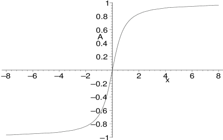
Let us present an example of this class of nonlinear sigma models to illustrate points raised in the previous section. From now on we shall use superpotential as the chiral scalar field of the nonlinear sigma model. Nonlinear sigma models with two isolated singularities within the holomorphically factorizble models can be put into the following form by rescaling and shift of field and coordinates

$$K_{AA^{*}}=\left|{1\over 1-A^{2}}\right|^{2},\qquad{\cal W}=A.$$ (2.20)

This model has two SUSY vacua at $A=\pm 1$ where the Kähler metric is singular. The BPS equation (2.11) for a wall connecting the vacuum $A=-1$ at $x=-\infty$ to the vacuum $A=1$ at $x=\infty$ reduces to

$${dA\over dx}=K^{AA^{*}}=\left|1-A^{2}\right|^{2}.$$ (2.21)

We can easily find the solution

$$x-x_{0}={1\over 4}\left({2A\over 1-A^{2}}+{\rm log}\left({1+A\over 1-A}\right)\right)$$ (2.22)

where the integration constant $x_{0}$ corresponds to the position of the wall. The solution with $x_{0}=0$ is illustrated in Fig.1. We can also generalize the model to the case of $n$ isolated singularities for the Kähler metric.

It is instrutive to map the above model into a linear sigma model by a holomorphic field redefinition from $A$ to $A^{\prime}$

$${dA^{\prime}\over dA}={1\over 1-A^{2}}.$$ (2.23)

The scalar field $A$ of the linear sigma model is given by

$$A^{\prime}={\rm arctanh}A.$$ (2.24)

The bosonic part of the linear sigma model equivalent to the nonlinear sigma model given in Eq.(2.20) reads

$${\cal L}_{\rm LSM}=-\partial_{\mu}A^{\prime*}\partial^{\mu}A^{\prime}-V(A^{\prime},A^{\prime*}),\qquad V(A^{\prime},A^{\prime*})={1\over|\cosh^{2}A^{\prime}|^{2}}.$$ (2.25)

The SUSY vacua $A=-1$ and $A=1$ of the nonlinear sigma model are mapped into $A^{\prime}=-\infty$ and $A^{\prime}=\infty$ respectively. The scalar potential is plotted as a function of $A^{\prime}$ along the real axis in Fig.2.

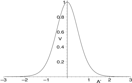
Figure 2: Scalar potential of the linear sigma model (2.25)

We see that the scalar potential $V(A^{\prime},A^{\prime*})$ of the linear sigma model vanishes only asymptotically at $A^{\prime}=\pm\infty$. One usually regards these vacua at infinity as the runaway vacua and discards them. The nonlinear sigma model in this example shows an advantage of revealing these vacua as legitimate SUSY vacua and moreover allowing the BPS wall solution connecting these two vacua. This particular model (2.25) was used to discuss the quantum tunneling problem [21] and properties of the ”vacuumless” model similar to this one have been studied [22]. The wall solution corresponds to the zero energy limit of the tunneling amplitude. There is a singularity of the scalar potential at $A^{\prime}=i\left({1\over 2}+n\right)\pi$ with an integer $n$. As shown in Fig.3, the singularities of Kähler metric at $A=\pm 1$ is mapped to infinity $A^{\prime}=\infty$ in $A^{\prime}$ plane, and that the singularity of the scalar potential at $A^{\prime}=i\left({1\over 2}+n\right)\pi$ is mapped to $A=\infty$ in $A$ plane. The variable in linear sigma model now becomes a periodic variable. This appearance of periodic variable carries an interesting phenomenon of possible winding number which is also noted in [23], [6]. Another interesting example of holomorphically factorizable model is given in appendix A to illustrate physical difference of the Kähler metric in discussing nonperturbative dynamics of ${\cal N}=1$ SUSY gauge theories.

$$\begin{array}[]{cc}\epsfbox{period-1a.eps}&\hskip 28.45274pt\epsfbox{period-1b.eps}\\ \mbox{\footnotesize(a) Nonlinear sigma model}&\hskip 28.45274pt\mbox{\footnotesize(b)Linear sigma model}\end{array}$$

Figure 3: Field space for linear and nonlinear sigma model. Solid, dashed, dotted lines with arrows in the $A^{\prime}$ plane are mapped to those corresponding lines in the $A$ plane.

3 Nonlinear sigma models with exact junction solutions

3.1 A linear sigma model with $Z_{3}$ BPS junction

In this section we study BPS junction configuration in nonlinear sigma models. Let us first review the exact BPS junction solution obtained in Refs.[13], [14]. The model is a toy model for the low-energy effective theory of the ${\cal N}=2$ $SU(2)$ gauge theory with a single flavor [25], [26]. It has $U(1)\times U(1)$ gauge symmetry and chiral scalar multiplets for “monopole” ${\cal M}$, “anti-monopole” $\bar{\cal M}$, “dyon” ${\cal D}$, “anti-dyon” $\bar{\cal D}$ and “quark” ${\cal Q}$, “anti-quark” $\bar{\cal Q}$ besides the “moduli” $\hat{T}$. Moreover the exact solution was obtained when the model possesses the $Z_{3}$ symmetry. It has also been recognized that the same exact solution can be obtained for the model with only chiral scalar superfields by eliminating the gauge interactions, identifying ${\cal M}=\bar{\cal M},\ {\cal D}=\bar{\cal D},\ {\cal Q}=\bar{\cal Q}$ and adjusting the parameters appropriately [14]. Therefore we can take this linear sigma model and ask if the BPS junction solution can be generalized to other models and/or other symmetries. There are four chiral scalar superfields ${\cal M}_{i},i=1,2,3$ and $\hat{T}$ with the minimal kinetic term. The linear sigma model with $Z_{3}$ symmetric junction solution can be reduced to the following form of superpotential after shift and rescaling of fields

$${\cal W}={1\over 2}\left[\sqrt{3}\hat{T}-\sum_{j=1}^{3}\left(\sqrt{3}\hat{T}-{\rm e}^{i{2\pi\over 3}j}\right){\cal M}_{j}^{2}\right].$$ (3.1)

There are three isolated SUSY vacua as depicted in Fig. 4

$$\hat{T}={1\over\sqrt{3}}{\rm e}^{i{2\pi\over 3}j},\quad{\cal M}_{j}=\pm 1,\quad{\cal M}_{k}=0,\;k\not=j,\qquad j=1,2,3.$$ (3.2)

$$\begin{array}[]{cc}\epsfbox{vacua-6.eps}&\hskip 28.45274pt\epsfbox{junct-3b.eps}\\ \mbox{\footnotesize(a) Vacua of $Z_{3}$ linear sigma model}&\hskip 28.45274pt\mbox{\footnotesize(b) $Z_{3}$ junction in the base space}\end{array}$$

Figure 4: $Z_{3}$ symmetric linear sigma model.

The ${1\over 4}$ BPS equation (2.11) is given by

$$2{\partial{\cal M}_{j}\over\partial z}=\left({\rm e}^{-i{2\pi\over 3}j}-\sqrt{3}\hat{T}^{*}\right){\cal M}_{j}^{*},$$ (3.4)

$$2{\partial\hat{T}\over\partial z}={\sqrt{3}\over 2}\left(1-\sum_{j=1}^{3}{\cal M}_{j}^{*2}\right)$$ (3.5)

where we have set the constant phase factor $\Omega_{-}=1$ in order to orient the wall separating the vacuum $\hat{T}={\rm e}^{\pm i{2\pi\over 3}}/\sqrt{3}$ along the negative real axis as shown in Fig. 4. It is convenient to define the following auxiliary quantities taking real values

$$f_{j}\equiv\exp\left({1\over 2}\left({\rm e}^{-i{2\pi\over 3}j}z+{\rm e}^{i{2\pi\over 3}j}z^{*}\right)\right),\qquad j=1,2,3.$$ (3.6)

which satisfy the following identity

$$\prod_{j=1}^{3}f_{j}=1.$$ (3.7)

The exact BPS solution for a junction connecting three vacua is given by [13]

$$\hat{T}={1\over\sqrt{3}}{\sum_{j=1}^{3}{\rm e}^{i{2\pi\over 3}j}f_{j}\over\sum_{k=1}^{3}f_{k}},\qquad{\cal M}_{j}={f_{j}\over\sum_{k=1}^{3}f_{k}}.$$ (3.8)

We have shown that the configuration (3.8) on a circle at infinity $|z|\rightarrow\infty$ reduces to a collection of three walls separating three vacuum regions which are represented by three straight line segments connecting three vacua in Fig. 4 [13], [14].

3.2 A nonlinear sigma model with BPS junction

We would like to construct a nonlinear sigma model which has an exact BPS solution of the junction. We observe that the junction solution is a mapping from a two-dimensional base space $x^{1},x^{2}$ to the complex scalar fields ${\cal M}_{j},j=1,2,3$ and $\hat{T}$. Therefore we can reexpress the complex scalar fields ${\cal M}_{j},j=1,2,3$ in favor of the complex coordinate $z=x^{1}+ix^{2}$ and then invert the relation between $\hat{T}$ and $z$ to express everything in favor of $\hat{T}$ eventually. In particular, we can express the right-hand side of the BPS equation for $\hat{T}$ in Eq.(3.5) solely in terms of $\hat{T}$ by this process. The resulting BPS equation can be interpreted as the BPS equation (2.11) in a nonlinear sigma model with appropriate superpotential and Kähler metric. In the present case, we can make use of the identity (3.7) and use real quantities $f_{1}$ and $f_{2}$ instead of coordinates $x^{1}$ and $x^{2}$ in the intermediate stage. Using Eqs.(3.5), (3.7), and (3.8), we obtain

$$2{\partial\hat{T}\over\partial z} \!\!\!= \!\!\!{\sqrt{3}\over 2}\left(1-\sum_{j=1}^{3}{\cal M}_{j}^{*2}\right)={\sqrt{3}\over 2}\left(1-{\sum_{j=1}^{3}f_{j}^{2}\over\left(\sum_{k=1}^{3}f_{k}\right)^{2}}\right)=\sqrt{3}{f_{1}f_{2}+f_{2}f_{3}+f_{3}f_{1}\over\left(\sum_{k=1}^{3}f_{k}\right)^{2}}$$ (3.9)

$$\!\!\!= \!\!\!\sqrt{3}{f_{1}f_{2}+{1\over f_{1}}+{1\over f_{2}}\over\left(f_{1}+f_{2}+{1\over f_{1}f_{2}}\right)^{2}}=\sqrt{3}{f_{1}f_{2}\left(f_{1}^{2}f_{2}^{2}+f_{1}+f_{2}\right)\over\left(f_{1}f_{2}\left(f_{1}+f_{2}\right)+1\right)^{2}}.$$

where we have eliminated $f_{3}$ by means of the identity (3.7). Similarly we can reexpress the field $\hat{T}=\hat{T}_{R}+i\hat{T}_{I}$ as

$$\sqrt{3}\hat{T}_{R}={-{f_{1}+f_{2}\over 2}+f_{3}\over\sum_{k=1}^{3}f_{k}}={-{f_{1}f_{2}(f_{1}+f_{2})\over 2}+1\over f_{1}f_{2}(f_{1}+f_{2})+1}$$ (3.10)

$$\sqrt{3}\hat{T}_{I}={{\sqrt{3}\over 2}(f_{1}-f_{2})\over f_{1}+f_{2}+{1\over f_{1}f_{2}}}={{\sqrt{3}\over 2}f_{1}f_{2}(f_{1}-f_{2})\over f_{1}f_{2}(f_{1}+f_{2})+1}.$$ (3.11)

Therefore we finally find that

$$2{\partial\hat{T}\over\partial z}={1\over\sqrt{3}}\left(1-3\hat{T}_{R}^{2}-3\hat{T}_{I}^{2}\right)={1\over\sqrt{3}}\left(1-|\sqrt{3}\hat{T}|^{2}\right).$$ (3.12)

The resulting equation should be identified with a ${1\over 4}$ BPS equation (2.11) for a nonlinear sigma model. We find that the superpotential is linear in $\hat{T}$ and the Kähler metric is nontrivial

$$K_{\hat{T}\hat{T}^{*}}={3\over 1-|\sqrt{3}\hat{T}|^{2}},\qquad{\cal W}=\sqrt{3}\hat{T}.$$ (3.13)

We emphasize that the above choice is not a matter of convenience, and that the holomorphy forces us to choose the superpotential as the chiral scalar superfield $\hat{T}$ itself except for the freedom of a possible proportionality constant ${\cal W}/\hat{T}$. The Kähler potential is given by

$$K(\hat{T},\hat{T}^{*})=\int^{3|\hat{T}|^{2}}{dx\over x}\log{1\over 1-x}.$$ (3.14)

From the above procedure, we see that the nonlinear sigma model with a single chiral scalar superfield is unique modulo usual freedom of holomorphic field redefinitions, if we require that it allows the exact junction (3.8) as the ${1\over 4}$ BPS solution.

By using a rescaled field $T\equiv\sqrt{3}\hat{T}$, we obtain the nonlinear sigma model

$${\cal L}_{{\rm NLSM}}=-{1\over 1-|T|^{2}}\partial_{\mu}T^{*}\partial^{\mu}T-\left(1-|T|^{2}\right).$$ (3.15)

We observe that the nonlinear sigma model has continuous vacua at $|T|=1$, corresponding to the continuous family of singularities of the Kähler metric. The moduli space has a topology of a circle.

Now we shall show that there are ${1\over 2}$ BPS wall solutions connecting any two arbitrary points in this moduli space. Since an orthogonal section of the ${1\over 2}$ BPS configuration should follow a straight line trajectory in the complex plane of the superpotential, we just need to construct a straight line connecting two vacua in the moduli space, thanks to our choice of the superpotential as the field variable. Let us define a variable taking a real value $-1\leq\tilde{T}\leq 1$ along the straight line connecting from $T={\rm e}^{i\alpha_{1}}$ and $T={\rm e}^{i\alpha_{2}}$ as shown in Fig. 5

$$T={{\rm e}^{i\alpha_{2}}+{\rm e}^{i\alpha_{1}}\over 2}+{{\rm e}^{i\alpha_{2}}-{\rm e}^{i\alpha_{1}}\over 2}\tilde{T}.$$ (3.16)

Then the ${1\over 2}$ BPS equations (2.11) and (2.12) for the wall reduce to

$${d\tilde{T}\over dx}=\sin{\alpha_{2}-\alpha_{1}\over 2}\left[1-\left(\tilde{T}\right)^{2}\right]$$ (3.17)

where we have taken the constant phase factor as $\Omega=i{\rm e}^{i{\alpha_{2}+\alpha_{1}\over 2}}$ in order to orient the wall along the $x=x^{1}$ direction. We can recognize the familiar BPS equation to give the wall solution and find

$$\tilde{T}=\tanh\left(x\sin{\alpha_{2}-\alpha_{1}\over 2}\right)$$ (3.18)

$$T={{\rm e}^{i\alpha_{2}}{\rm e}^{x\sin{\alpha_{2}-\alpha_{1}\over 2}}+{\rm e}^{i\alpha_{1}}{\rm e}^{-x\sin{\alpha_{2}-\alpha_{1}\over 2}}\over{\rm e}^{x\sin{\alpha_{2}-\alpha_{1}\over 2}}+{\rm e}^{-x\sin{\alpha_{2}-\alpha_{1}\over 2}}}.$$ (3.19)

Figure 5: A BPS wall connecting any two vacua

More surprisingly, we can show that there exist exact ${1\over 4}$ BPS junction solutions connecting any number of ordered points ${\rm e}^{i\alpha_{j}},j=1,\cdots,N$ in the moduli space as shown in Fig. 6.

$$\begin{array}[]{cc}\epsfbox{vacua-4.eps}&\hskip 28.45274pt\epsfbox{junct-1.eps}\\ \mbox{\footnotesize(a) Moduli space and $N$ vacua for a junction.}&\hskip 28.45274pt\mbox{\footnotesize(b) $N$ junction configuration. }\end{array}$$

Figure 6: Nonlinear sigma model with single chiral scalar superfield (3.15)

To obtain the junction solution, let us define the following auxiliary quantities $f_{j}$ generalized from Eq.(3.6)

$$f_{j}\equiv\exp\left({1\over 2}\left({\rm e}^{-i\alpha_{j}}z+{\rm e}^{i\alpha_{j}}z^{*}\right)\right),\qquad j=1,\cdots,N.$$ (3.21)

Let us define an auxiliary variable $\eta$ as

$$\eta\equiv 2\log\left(\sum_{j=1}^{N}f_{j}\right).$$ (3.22)

Then we obtain

$${\partial\eta\over\partial z}={\sum_{k=1}^{N}{\rm e}^{-i\alpha_{k}}f_{k}\over\sum_{j=1}^{N}f_{j}},\qquad{\partial^{2}\eta\over\partial z\partial z^{*}}={1\over 2}\left[1-\left|{\partial\eta\over\partial z}\right|^{2}\right],$$ (3.23)

If we take the following Ansatz

$$T={\partial\eta\over\partial z^{*}}={\sum_{k=1}^{N}{\rm e}^{i\alpha_{k}}f_{k}\over\sum_{j=1}^{N}f_{j}},$$ (3.24)

we find that the field $T$ satisfies the ${1\over 4}$ BPS equation (2.11) for the nonlinear sigma model (3.15) with the Kähler metric $K_{TT^{*}}=1/(1-|T|^{2})$ and the superpotential ${\cal W}=T$

$$2{\partial T\over\partial z}=1-\left|{\partial\eta\over\partial z}\right|^{2}=1-\left|T\right|^{2}.$$ (3.25)

To clarify the physical meaning of this solution, we evaluate the asymptotic behavior at infinity. Let us define a coordinate system rotated by an angle $\theta$, $\hat{z}\equiv{\rm e}^{-i\theta}z=\hat{x}+i\hat{y}$. As shown in Fig. 7, the negative $\hat{y}$ axis of the rotated coordinates is at the angle $\hat{\theta}=\theta-\pi/2$. Let us first take the asymptotic limit $\hat{y}\rightarrow-\infty$ along a generic direction satisfying

$${\alpha_{j-1}+\alpha_{j}\over 2}<\hat{\theta}<{\alpha_{j}+\alpha_{j+1}\over 2}.$$ (3.26)

Figure 7: The directions of asymptotic limits of the $N$-juncion configuration.

We find that $f_{j}$ is dominant compared to all the other $f_{k}$’s and that the $j$-th vacuum is reached asymptotically $\hat{y}\rightarrow-\infty$

$$f_{j}>>f_{k},\quad k\not=j,\qquad T\rightarrow{\rm e}^{i\alpha_{j}}.$$ (3.27)

Let us next take the asymptotic limit $\hat{y}\rightarrow-\infty$ along the direction $\hat{\theta}=(\alpha_{j+1}+\alpha_{j})/2$ which corresponds to the boundary of the two vacua $T={\rm e}^{i\alpha_{j}}$ and $T={\rm e}^{i\alpha_{j+1}}$, as given by the condition (3.26). The auxiliary quantities become for a general $k$

$$f_{k}=\exp\left[-\hat{y}\cos\left(\alpha_{k}-{\alpha_{j}+\alpha_{j+1}\over 2}\right)+\hat{x}\sin\left(\alpha_{k}-{\alpha_{j}+\alpha_{j+1}\over 2}\right)\right],$$ (3.28)

$$f_{j} \!\!\!= \!\!\!\exp\left[-\hat{y}\cos\left({\alpha_{j+1}-\alpha_{j}\over 2}\right)-\hat{x}\sin\left({\alpha_{j+1}-\alpha_{j}\over 2}\right)\right],$$

$$f_{j+1} \!\!\!= \!\!\!\exp\left[-\hat{y}\cos\left({\alpha_{j+1}-\alpha_{j}\over 2}\right)+\hat{x}\sin\left({\alpha_{j+1}-\alpha_{j}\over 2}\right)\right]$$ (3.29)

for $j$ and $j+1$ in particular. In the limit $\hat{y}\rightarrow-\infty$, we find

$$0\leq f_{k}\ll f_{j},f_{j+1},$$ (3.30)

Therefore we obtain the asymptotic behavior for a wall connecting two vacua ${\rm e}^{i\alpha_{j}}$ to ${\rm e}^{i\alpha_{j+1}}$

$$T\rightarrow{{\rm e}^{i\alpha_{j+1}}{\rm e}^{x\sin{\alpha_{j+1}-\alpha_{j}\over 2}}+{\rm e}^{i\alpha_{j}}{\rm e}^{-x\sin{\alpha_{j+1}-\alpha_{j}\over 2}}\over{\rm e}^{x\sin{\alpha_{j+1}-\alpha_{j}\over 2}}+{\rm e}^{-x\sin{\alpha_{j+1}-\alpha_{j}\over 2}}},\quad\hat{y}\rightarrow-\infty,$$ (3.31)

which can be compared with the domain wall solution in Eq.(3.19). Thus we find that the domain wall connecting from the vacuum ${\rm e}^{i\alpha_{j}}$ to the vacuum ${\rm e}^{i\alpha_{j+1}}$ extends along a direction in the base space $z$ which is orthogonal to the line connecting from the vacuum ${\rm e}^{i\alpha_{j}}$ to the vacuum ${\rm e}^{i\alpha_{j+1}}$ in the complex $T$ plane. Moreover the junction solution maps the asymptotic infinity of the base space $z$ to a collection of line segments connecting the vacua in conformity with the theorem (2.15) as shown in Fig. 6.

The kinetic term of the nonlinear sigma model is nonnegative definite only for $|T|\leq 1$. It is interesting to observe that the moduli space $|T|=1$ of the nonlinear sigma model forms a natural boundary of the field space beyond which the kinetic term of the nonlinear sigma model is no longer positive definite. The curvature of the metric $K_{TT^{*}}=1/(1-|T|^{2})$ is given by

$$R=2R_{TT^{*}}\left(1-|T|^{2}\right)=-2R_{TT^{*}TT^{*}}\left(1-|T|^{2}\right)^{2}={-2\over 1-|T|^{2}}.$$ (3.32)

Another peculiar feature of the nonlinear sigma model (3.15) is that the boundary condition can be deformed continuously since the moduli space of vacua is continuous. The walls and junctions are stable as long as the boundary condition is fixed. However, the adiabatic change of the boundary condition can make the adiabatic deformation of the walls and junctions.

4 Nonlinear sigma models with discrete vacua and junction solution

If one wants to prevent the continuous deformation of walls and junctions in the nonlinear sigma model (3.25), we can invent another model with discrete vacua. We shall work out the model which has the $N$-junction as a solution of ${1\over 4}$ BPS equation. Let us introduce the chiral scalar superfields ${\cal M}_{j},j=1,\cdots,N$ besides the chiral scalar superfield $T$. We assume the minimal kinetic term for these additional fields ${\cal M}_{j}$. However, we leave the Kähler metric $K_{TT^{*}}$ of the field $T$ to be an arbitray function of $T,T^{*}$ and will determine it by requiring that the model possesses a $N$-junction as a solution of the ${1\over 4}$ BPS equation. We assume a generalization of the superpotential in Eq.(3.1)

$${\cal W}={1\over 2}\left[T-\sum_{j=1}^{N}\left(T-{\rm e}^{i\alpha_{j}}\right){\cal M}_{j}^{2}\right]$$ (4.1)

where the parameters $\alpha_{j},\;j=1,\cdots,N$ specify the position of discrete vacua as we show below, and becomes $\alpha_{j}=2\pi j/N$ for the $Z_{N}$ symmetric case.

The SUSY vacuum condition (2.8) gives two conditions in this model

$$\left({\rm e}^{i\alpha_{j}}-T\right){\cal M}_{j}=0,\qquad j=1,\cdots,N,$$ (4.2)

$$K^{TT^{*}}{1\over 2}\left|1-\sum_{j=1}^{N}{\cal M}^{2}_{j}\right|^{2}=0.$$ (4.3)

We find that there are two types of the SUSY vacua as in Fig.6(a):

1. The $j$-th condition (4.2) is satisfied if the field T takes a particular value $T={\rm e}^{i\alpha_{j}}$ for an integer $j$. Then the other conditions (4.2) imply ${\cal M}_{k}=0$ for $k\not=j$. Assuming that the Kähler metric is not singular at the point $T={\rm e}^{i\alpha_{j}}$, the second condition (4.3) is only satisfied by ${\cal M}_{j}=\pm 1$.

   $$T={\rm e}^{i\alpha_{j}},\quad{\cal M}_{j}=\pm 1,\quad{\cal M}_{k}=0,\;k\not=j,\qquad j=1,\cdots,N.$$ (4.4)

   We will check later that the Kähler metric is indeed not singular at this point. This is the $N$ discrete SUSY vacua given by stationary points of the superpotential as shown in Fig. 6(a).

2. If $T\not={\rm e}^{i\alpha_{j}},\;j=1,\cdots,N$, all the other fields have to vanish ${\cal M}_{j}=0$ to satisfy Eq.(4.2). The other condition (4.3) can only be satisfied by a singularity of the Kähler metric

   $$K_{TT^{*}}=\infty.$$ (4.5)

The ${1\over 4}$ BPS equations (2.11) for ${\cal M}_{j}$ and $T$ are given by

$$2{\partial{\cal M}_{j}\over\partial z}=\left({\rm e}^{-i\alpha_{j}}-T^{*}\right){\cal M}_{j}^{*},$$ (4.6)

$$2{\partial T\over\partial z}=K^{TT^{*}}{1\over 2}\left(1-\sum_{j=1}^{N}{\cal M}_{j}^{*2}\right).$$ (4.7)

Using the auxiliary quantities $f_{j}$ defined in Eq.(3.21), we assume the following Ansatz for the junction

$$T={\sum_{j=1}^{N}{\rm e}^{i\alpha_{j}}f_{j}\over\sum_{k=1}^{N}f_{k}},\qquad{\cal M}_{j}={f_{j}\over\sum_{k=1}^{N}f_{k}}.$$ (4.8)

By using identities

$${\partial f_{j}\over\partial z}={1\over 2}{\rm e}^{-i\alpha_{j}}f_{j},$$ (4.9)

$${\partial\over\partial z}\left({f_{j}\over\sum_{k=1}^{N}f_{k}}\right) \!\!\!= \!\!\!{1\over 2}{{\rm e}^{-i\alpha_{j}}f_{j}\over\sum_{k=1}^{N}f_{k}}-{f_{j}\over 2}{\sum_{m}{\rm e}^{-i\alpha_{m}}f_{m}\over\left(\sum_{k=1}^{N}f_{k}\right)^{2}}={f_{j}\over\sum_{k=1}^{N}f_{k}}{1\over 2}\left({\rm e}^{-i\alpha_{j}}-T^{*}\right)$$ (4.10)

we find that the ${1\over 4}$ BPS equation for ${\cal M}_{j}$ in Eq.(4.6) is satisfied. Then the remaining ${1\over 4}$ BPS equation for $T$ is also satisfied if and only if the Kähler metric of the field $T$ is given by

$$K_{TT^{*}} \!\!\!= \!\!\!{{1\over 2}\left(1-\sum_{j=1}^{N}{\cal M}_{j}^{*2}\right)\over 2{\partial T\over\partial z}}={1-{\sum_{j=1}^{N}f_{j}^{2}\over\left(\sum_{k=1}^{N}f_{k}\right)^{2}}\over 2\left(1-{|\sum_{l=1}^{N}{\rm e}^{i\alpha_{l}}f_{l}|^{2}\over\left(\sum_{m=1}^{N}f_{m}\right)^{2}}\right)}$$ (4.11)

$$\!\!\!= \!\!\!{1-{\sum_{j=1}^{N}f_{j}^{2}\over\left(\sum_{k=1}^{N}f_{k}\right)^{2}}\over 2\left(1-|T|^{2}\right)}={2{\sum_{j<l}f_{j}f_{k}\over\left(\sum_{k=1}^{N}f_{k}\right)^{2}}\over 2\left(1-|T|^{2}\right)}.$$

Here we have expressed the metric in terms of the auxiliary quantities $f_{j}$ as an intermediate step. The numerator of the right-hand side can be expressed in terms of the $T=T_{R}+iT_{I}$, since $f_{j}$ are given in terms of $z$ which can be expressed in terms of $T_{R}$ and $T_{I}$. Therefore we have solved the ${1\over 4}$ BPS equations and obtained the Kähler metric of the nonlinear sigma model implicitly through Eqs.(3.21), (4.8), and (4.11). It is gratifying to find that the resulting Kähler metric is real. This is a nontrivial requirement which should be imposed on the Kähler metric. The asymptotic behavior of the solution is precisely the same as in the previous section. Therefore we have found the ${1\over 4}$ BPS junction solution connecting $N$ discrete vacua.

We now examine the properties of the Kähler metric (4.11). The singularity can occur only on a circle $|T|=1$. However, the junction solution can never touch the circle as long as $z$ is finite. The circle can be reached only asymptotically as $|z|\rightarrow\infty$. In fact, the analysis in the previous section shows that the junction solution approaches asymptotically along a generic direction to one of the discrete vacua, say ${\rm e}^{i\alpha_{j}}$. On the other hand, the numerator is such that it also vanishes precisely at these vacua and the Kähler metric becomes finite at the discrete vacua

$$K_{TT^{*}}\rightarrow{1\over 2\left(1-\cos(\alpha_{j}-\alpha_{j-1})\right)},$$ (4.12)

if the nearest vacuum to ${\rm e}^{\alpha_{j}}$ is at ${\rm e}^{\alpha_{j-1}}$. If the nearest vacuum is at ${\rm e}^{\alpha_{j+1}}$ instead, we should replace $\alpha_{j-1}$ by $\alpha_{j+1}$. This result shows that the Kähler metric is in fact nonsigular as we have assumed in analyzing the SUSY vacua. The junction asymptotically along the wall direction becomes a wall solution. In our solution, we have already shown in the previous section that the wall is mapped to a straight line segments connecting adjacent vacua in the $T$ plane. The Kähler metric takes the value (4.12) along the straight line corresponding to the wall connecting the vacua $T={\rm e}^{\alpha_{j-1}}$ and $T={\rm e}^{\alpha_{j}}$. Let us call $R=\{T(z,z^{*})\in{\bf C},z\in{\bf C}\}$ the image of the entire real space $z$ by the map $T(z,z^{*})$ defined by the junction solution (4.8). Summarizing the properties of the Kähler metric, we find

1. The Kähler metric is real and positive in $R$.

2. The Kähler metric is never singular in $R$.

3. The field $T$ can approach asymptotically to the unit circle only at the discrete vacuum $T={\rm e}^{i\alpha_{j}}$ where the Kähler metric is finite.

4. The asymptotic value of the junction solution is mapped to a straight line segments connecting these discrete vacua.

5. At the origin of the base space, the auxiliary quantity becomes $f_{j}=1$. In the case of $Z_{N}$ symmetric model, the field takes values $T=0,{\cal M}_{j}=1/N$ and the Kähler metric takes a value $K_{TT^{*}}=(N-1)/(2N)$.

These results suggest that $R$ is a polygon with the $N$ discrete vasua as vertices. It is interesting to observe that the moduli space is divided into several discrete stationary points and singular arcs. We expect that the kinetic term is positive definite in $|T|\leq 1$, and that the natural domain of definition for our nonlinear sigma model is $|T|\leq 1$, which turn out to be the case in models that we are going to analyze more explicitly.

Let us evaluate the Kähler metric as a function of $T$ more explicitly. For that purpose, we shall first take the $Z_{N}$ symmetric case. The model with junction starts from $N=3$. The model with $N=3$ turn out to give a minimal kinetic term $K_{TT^{*}}=1$ and hence reduces to our original model in sect.3.1. The next model is $N=4$. We find that the model in fact gives a nonlinear sigma model for the field $T$ as

$$K_{TT^{*}}={1\over 2(1-|T|^{2})}\left[{3\over 4}-{1\over 2}|T|^{2}-{1\over 16}\left(T^{4}+T^{*4}\right)-{1\over 8}|T|^{4}\right].$$ (4.13)

$$\begin{array}[]{cc}\epsfbox{vacua-5a.eps}&\hskip 28.45274pt\epsfbox{junct-2.eps}\\ \mbox{\footnotesize(a) Vacua of the $Z_{4}$ symmetric nonlinear sigma model}&\hskip 28.45274pt\mbox{\footnotesize(b) $Z_{4}$ junction}\end{array}$$

Figure 8: Nonlinea sigma model with $Z_{4}$ symmetric junction.

The explicit representation (4.13) in terms of $T$ shows that there is a locus of zeros which touches the unit circle precisely at the four discrete points $T={\rm e}^{i{2\pi\over 4}j},j=1,\cdots,4$. This concrete example shows our general analysis clearly: the Kähler metric is singular along four arcs separated by discrete stationary points of the superpotential $T={\rm e}^{i{2\pi\over 4}j},j=1,\cdots,4$ where the Kähler metric is finite. The region between the circle $|T|=1$ and the outer curve touching the circle at $T=1,i,-1,-i$ gives the region of negative kinetic term as shown in Fig. 8(a). In this model, we have also a continuous moduli space consisting of the arcs of singularities of the Kähler metric. However, even if we attempt to make a wall and/or a junction solution connecting these vacua of singularities, we find that the BPS equations are not satisfied by Ansatz similar to our previous one in Eqs.(3.24) or (4.8), since $T$ now has a nonlinear kinetic term in our model. It is possible that there may exist wall or junction solutions connecting these singularities of the Kähler metric. Even if they exist, however, these solutions cannot be adiabatically deformed to our solution, since the other fields ${\cal M}$ take different values in two types of vacua as shown in Eqs.(4.4) and (4.5).

As another example, we shall give a model without the $Z_{N}$ symmetry. Let us take three “matter” fields ${\cal M}_{j},j=1,2,3$ besides $T$. We choose the superpotential (4.1) with $\alpha_{1}=\pi/2,\alpha_{2}=-\pi/2,\alpha_{3}=0$. Then we have three discrete vacua at asymmetric points $T=1,i,-i$ on the unit circle as shown in Fig. 9.

$$\begin{array}[]{cc}\epsfbox{vacua-7a.eps}&\hskip 28.45274pt\epsfbox{junct-4.eps}\\ \mbox{\footnotesize(a) Vacua at $T=1,i,-i$ of a nonlinear sigma model. }&\hskip 28.45274pt\mbox{\footnotesize(b) Asymmetric $3$-junction. }\end{array}$$

Figure 9: Nonlinear sigma model with asymmetric $3$-junction.

We find that the Kähler metric in Eq.(4.11) becomes in this model

$$K_{TT^{*}}={1\over 4(1-|T|^{2})}\left(1+T+T^{*}-2|T|^{2}-{T^{2}+T^{*2}\over 2}\right).$$ (4.16)

The Kähler metric again has a general feature: it is finite at the discrete vacua which separate the arcs of singular points of the Kähler metric as shown in Fig. 9. The kinetic term is negative in the region between the circle $|T|=1$ and the ellipse touching the circle at three vacua $T=1,i,-i$ as shown in Fig. 9.

Acknowledgments

One of the authors (N.S.) thanks a discussion with Tohru Eguchi, Kazuo Fujikawa, and Yoichi Kazama. This work is supported in part by Grant-in-Aid for Scientific Research from the Japan Ministry of Education, Science and Culture 13640269, and those for the Priority Area 707.

Appendix A Example of nontrivial Kähler metric and SUSY vacua

In this appendix, we shall present as another interesting example of holomorphically factorizable model, a toy model which mimics the difference in physical consequences due to the choice of the Kähler metric in discussing the nonperturbative dynamics of ${\cal N}=1$ SUSY theories. The $SU(N_{c})$ SUSY gauge theories is known to have gaugino condensation with $N_{c}$ distinct chirally asymmetric vacua. This gaugino condensation induces a nonperturbative superpotential. There have been a lot of discussion about the wall solutions connecting these vacua. We shall denote the moduli field by a chiral scalar superfield $\Phi^{\prime}$ corresponding to a color singlet field. Let us take the case $N_{c}=2n$ for simplicity and mimic the $2n$ distinct vacua as stationary points at $A^{\prime}={m}{\rm e}^{i{2\pi\over 2n}k},\;k=0,1,\cdots,2n-1$ of the superpotential

$${\cal W}^{(1)}_{\rm np}(\Phi^{\prime})={m^{2}}\Phi^{\prime}\left(1-{1\over 2n+1}\left({\Phi^{\prime}\over m}\right)^{2n}\right).$$ (A.1)

The ${\cal N}=1$ SUSY is not powerful enough to determine the kinetic term of the “moduli” field $\Phi^{\prime}$. Usually one assumes that $\Phi^{\prime}$ has a minimal kinetic term. Then the bosonic part of the Lagrangian with the minimal kinetic term and with the nonperturbative superpotential (A.1) is given by

$${\cal L}^{(1)}=-\partial_{\mu}A^{\prime*}\partial^{\mu}A^{\prime}-\left|{d{\cal W}^{(1)}_{\rm np}\over dA^{\prime}}\right|^{2}=-\partial_{\mu}A^{\prime*}\partial^{\mu}A^{\prime}-\left|m^{2}\left(1-\left({A^{\prime}\over m}\right)^{2n}\right)\right|^{2}.$$ (A.2)

We shall refer this model as model one. The vacua of the model one in the complex $A^{\prime}$ plane are illustrated in Fig.10(a). Numerical evidence showed that there are wall solutions connecting the adjacent vacua at least [9].

$$\begin{array}[]{cc}\epsfbox{vacua-1.eps}&\hskip 28.45274pt\epsfbox{vacua-2.eps}\\ \mbox{\footnotesize(a)Vacua in linear sigma model}&\hskip 28.45274pt\mbox{\footnotesize(b)Vacua in nonlinear sigma model}\end{array}$$

Figure 10:

Another school of thought for the kinetic term of the moduli field assumes a nonlinear kinetic term. This is suggested by an idea that the moduli field is a color singlet composed of a bilinear of colored field. To illustrate the effect of nonlinear kinetic term, let us suppose that the moduli field $\Phi$ in this second model corresponds to the square of a chiral scalar superfield $\Phi^{\prime}$ with a minimal kinetic term

$$\Phi=\Phi^{\prime 2}/m$$ (A.4)

where a parameter $m$ of mass dimension one is used to make the dimension of scalar field canonical. We shall also assume that the nonperturbative superpotential has $n=N_{c}/2$ distinct stationary points at $A={m}{\rm e}^{i{2\pi\over n}k},\;k=0,1,\cdots,n-1$ and becomes

$${\cal W}^{(2)}_{\rm np}(A)={m^{2}}A\left(1-{1\over n+1}\left({A\over m}\right)^{n}\right)$$ (A.5)

in conformity with the fact that the two stationary points in $A^{\prime}$ are mapped into one point in $A$.

The bosonic part of the Lagrangian becomes in this case

$${\cal L}^{(2)} \!\!\!= \!\!\!-K_{AA^{*}}\partial_{\mu}A^{*}\partial^{\mu}A-K^{AA^{*}}\left|{d{\cal W}^{(2)}_{\rm np}\over dA}\right|^{2}$$ (A.6)

$$\!\!\!= \!\!\!-\left|{1\over 2}\sqrt{m\over A}\right|^{2}\partial_{\mu}A^{*}\partial^{\mu}A-\left|2\sqrt{A\over m}\right|^{2}\left|{m^{2}}\left(1-\left({A\over m}\right)^{n}\right)\right|^{2}.$$

We shall refer this model as two. In this case of the nonminimal kinetic term, we have an additional SUSY vacuum at the singularity of the Kähler metric at $A=0$ besides the already existing $N_{c}$ SUSY vacua at the stationary point of the superpotential. This additional SUSY vacuum mimics the so-called chirally symmetric vacuum. The physical difference of two models of nonperturbative dynamimcs originates from the different assumption on the Kähler potential which is not well-constrained in the ${\cal N}=1$ SUSY field theories.

References

- [1] S. Dimopoulos and H. Georgi, Nucl. Phys. B193 (1981) 150; N. Sakai, Z. f. Phys. C11 (1981) 153; E. Witten, Nucl. Phys. B188 (1981) 513; S. Dimopoulos, S. Raby, and F. Wilczek, Phys. Rev. D24 (1981) 1681.
- [2] N. Arkani-Hamed, S. Dimopoulos and G. Dvali, Phys. Lett. B429 (1998) 263 [hep-ph/9803315]; I. Antoniadis, N. Arkani-Hamed, S. Dimopoulos and G. Dvali, Phys. Lett. B436 (1998) 257 [hep-ph/9804398].
- [3] L. Randall and R. Sundrum, Phys. Rev. Lett. 83 (1999) 3370 [hep-ph/9905221]; Phys. Rev. Lett. 83 (1999) 4690 [hep-th/9906064].
- [4] G. Dvali and M. Shifman, Phys. Lett. B475 (2000) 295 [hep-ph/0001072]; E.A. Mirabelli and M.E. Peskin, Phys. Rev. D58 (1998) 065002 [hep-th/9712214] ; D.E. Kaplan, G.D. Kribs and M. Schmaltz, Phys. Rev. D62 (2000) 035010 [hep-ph/9911293]; Z. Chacko, M.A. Luty, A.E. Nelson and E. Ponton, JHEP 0001 (2000) 003 [hep-ph/9911323] ; T. Kobayashi and K. Yoshioka, Phys. Rev. Lett. 85 (2000) 5527 [hep-ph/0008069]; Z. Chacko and M.A. Luty, JHEP 0105 (2001) 067 [hep-ph/0008103] ; N. Arkani-Hamed, L.J. Hall, D. Smith and N. Weiner, Phys. Rev. D63 (2000) 056003 [hep-ph/9911421] ; D.E. Kaplan and T.M.P. Tait, JHEP 0006 (2000) 020 [hep-ph/0004200].
- [5] N. Maru, N. Sakai, Y. Sakamura, and R. Sugisaka, Phys. Lett. B496 (2000) 98, [hep-th/0009023].
- [6] N. Maru, N. Sakai, Y. Sakamura, and R. Sugisaka, “Simple SUSY Breaking Mechanism by Coexisting Walls ”, [hep-th/0107204].
- [7] E. Witten and D. Olive, Phys. Lett. B78 (1978) 97.
- [8] M. Cvetic, S. Griffies and S. Rey, Nucl. Phys. B381 (1992) 301 [hep-th/9201007].
- [9] G. Dvali and M. Shifman, Phys. Lett. B396 (1997) 64 [hep-th/9612128]; Nucl. Phys. B504 (1997) 127 [hep-th/9611213]; A. Kovner, M. Shifman, and A. Smilga, Phys. Rev. D56 (1997) 7978 [hep-th/9706089]; A. Smilga and A. Veselov, Phys. Rev. Lett. 79 (1997) 4529 [hep-th/9706217]; B. Chibisov and M. Shifman, Phys. Rev. D56 (1997) 7990; V. Kaplunovsky, J. Sonnenschein, and S. Yankielowicz, Nucl. Phys. B552 (1999) 209 [hep-th/9811195]; B. de Carlos and J. M. Moreno, Phys. Rev. Lett. 83 (1999) 2120 [hep-th/9905165]; G. Dvali, G. Gabadadze, and Z. Kakushadze, Nucl. Phys. B493 (1997) 148, [hep-th/9901032]; J. Edelstein, M.L. Trobo, F. Brito and D. Bazeia, Phys. Rev. D57 (1998) 7561 [hep-th/9707016]; M. Naganuma and M. Nitta, Prog. Theor. Phys.105(2001)501 [hep-th/0007184].
- [10] E. R. C. Abraham and P. K. Townsend, Nucl. Phys. B351 (1991) 313 ; M. Cvetic, F. Quevedo and S. Rey, Phys. Rev. Lett. 67 (1991) 1836.
- [11] G. Gibbons and P. Townsend, Phys. Rev. Lett. 83 (1999) 1727 [hep-th/9905196];
- [12] S.M. Carroll, S. Hellerman and M. Trodden, Phys. Rev. D61 (2000) 065001 [hep-th/9905217]; P.M. Saffin, Phys. Rev. Lett. 83 (1999) 4249-4252 [hep-th/9907066].
- [13] H. Oda, K. Ito, M. Naganuma and N. Sakai, Phys. Lett. B471 (1999) 148 [hep-th/9910095].
- [14] K. Ito, M. Naganuma, H. Oda and N. Sakai, Nucl. Phys. B586 (2000) 231 [hep-th/0004188]; Nucl. Phys. Proc. Suppl. 101 (2001) 304 [hep-th/0012182].
- [15] A. Gorsky and M. Shifman, Phys. Rev. D61 (2000) 085001 [hep-th/9909015]; Nucl. Phys. B586 (2000) 231 [hep-th/0004188]; D. Binosi and T. ter Veldhuis, Phys. Lett. B476 (2000) 124 [hep-th/9912081]; S. Nam and K. Olsen, JHEP 0008 (2000) 001 [hep-th/0002176].
- [16] L. Alvarez-Gaumé and D.Z. Freedman, Comm. Math. Phys. 91 (1983) 87; E.R.C. Abraham and P.K. Townsend, Phys. Lett. B291 (1992) 85; ibid. B295 (1992) 225.
- [17] J.P. Gauntlet, D. Tong and P.K. Townsend, Phys. Rev. D63 (2001) 085001 [hep-th/0007124]; J.P. Gauntlet, R. Portugues, D. Tong and P.K. Townsend, Phys. Rev. D63 (2001) 085002 [hep-th/0008221]; J.P. Gauntlet, D. Tong and P.K. Townsend, Phys. Rev. D64 (2001) 25010 [hep-th/0107228].
- [18] G. Sierra and P.K. Townsend, Nucl. Phys. B233 (1984) 289.
- [19] J. Sherk and J.H. Schwarz, Phys. Lett. B82 (1979) 60.
- [20] M. Naganuma, M. Nitta, and N. Sakai, “BPS lumps and their intersections in SUSY nonlinear sigma models” hep-th/0108133.
- [21] W.H. Miller, Adv. Chem. Phys. 25 (1974) 69.
- [22] I. Cho and A. Vilenkin, Phys. Rev. D59 (1999) 063510 [hep-th/9808092]; D. Bazeia, Phys. Rev. D60 (1999) 067705 [hep-th/9905184].
- [23] X. Hou, A. Losev, and M. Shifman, Phys. Rev. D61 (2000) 085005 [hep-th/9910071]; D. Binosi, M. Shifman and T. ter Veldhuis, Phys. Rev. D63 (2001) 025006 [hep-th/0006026].
- [24] J. Wess and J. Bagger, “Supersymmetry and Supergravity”, 1991, Princeton University Press.
- [25] N. Seiberg and E. Witten, Nucl. Phys. B426 (1994) 19; Nucl. Phys. B431 (1994) 484.
- [26] K. Intriligator and N. Seiberg, Nucl. Phys. B431 (1994) 551.