Forces between stable non-BPS branes

Abstract

As a step toward constructing realistic brane world models in string theory, we consider the interactions of a pair of non-BPS branes. We construct a dyonic generalization of the non-BPS branes first constructed by Bergman, Gaberdiel and Sen as orbifolds of D-branes on $T^{4}/\mathbb{Z}_{2}$. The force between a dyonic brane and an electric brane is computed and is found to vanish at a nontrivial critical separation. This equilibrium point is unstable. For smaller separations the branes coalesce to form a composite dyonic state, while for larger separations the branes run off to infinity. We suggest generalizations that will lead to potentials with stable local minima.

I Introduction

The existence of compact extra dimensions with sizes of order a millimeter appears to be consistent with all known experiments AHpheno . If true, the fundamental scale for physics may lie in the range $10-100$ TeV, and the hierarchy problem becomes explaining why the size of these extra dimensions is so large. For this new view to be consistent, one must postulate that the Standard Model fields are confined to a hypersurface in this higher dimension geometry – a “brane-world” extradlist . This idea is well-motivated in the context of string theory, where D-branes play exactly this role. A wide variety of gauge groups and matter content can be found as exact string theory compactifications (see stringcom ; nonbpslist for some reviews).

However we are still a long way off from reproducing the known Standard Model (with no other light fields) as an exact compactification of string theory. A step in this direction was taken in Sen0 where stable non-supersymmetric D-brane states were constructed in orbifolds of Type II string theory. Similar constructions developing more realistic gauge and matter contents followed (see nonbpslist for a review). However these compactifications are always accompanied by unwanted light fields associated with rescaling the sizes of internal dimensions (or the dilaton, which in turn is related to the size of an 11th direction in the M-theory viewpoint). These light fields are often referred to as radions.

At the phenomenological level, suggestions for stabilizing radion fields have been made in ahstab ; branecrystal . In particular, in branecrystal we showed the hierarchy problem could be solved by having a crystal structure in the internal dimensions, involving a large number of branes. For this to work, the forces between branes must balance at some finite critical radius, of order the fundamental length scale. In this paper we will take a step toward realizing this mechanism as an exact solution of string theory.

We will begin by generalizing the non-BPS branes of Ber1 ; Senrev (see also L1 ) to carry additional charge with respect to a $p-1$ form field strength. The interaction potential between such a dyonic brane and a purely electrically charged brane takes a highly nontrivial form that does indeed display an extremum at finite brane separation. Unfortunately for the example constructed here, this extremum is a local maximum. The branes may either run off to infinite separation, or they may coalesce. We conjecture the branes will form a stable composite dyonic state. Similar bound states have been discussed for pairs of pure electric case in lambertsachs . A supergravity solution for a stack of a large number of electric or magnetic branes has been constructed in gian . We suggest that the inclusion of other types of brane charge will lead to a true stable minimum.

To describe the non-BPS branes considered in this paper we employ the boundary state formalism. Such methods provide a convenient calculational tool for computing the potential between a pair of D-branes. Specifically for a pair of D-branes described by the boundary states $|D_{1}\rangle$ and $|D_{2}\rangle$ respectively, the potential between them is given by

$$V_{1-2}=-\langle D_{1}|{\cal D}|D_{2}\rangle$$ (1)

where ${\cal D}$ is the closed string propagator

$${\cal D}=\frac{\alpha^{\prime}}{4\pi}\int_{|z|\leq 1}\frac{d^{2}z}{|z|^{2}}z^{L_{0}}\bar{z}^{\tilde{L}_{0}}.$$ (2)

In the open string description of D-branes, one would instead have to compute the 1-loop partition function - or annulus diagram - with the open string endpoints on either brane. The advantage of the boundary state formalism is its universality. Once a boundary state is known one need only plug into (1) to find the potential between a pair of branes. In the open string description one must recompute the mode expansion for the open string each time one of the D-branes ($|D_{1,(2)}\rangle$) is changed as well as find the corresponding projection operator to be inserted in the partition function. The boundary state formalism has been applied in a variety of cases to study the properties of non-BPS branes (some reviews may be found in boundarystate ; diVLic ; diVLic2 ; L5 ).

II Constructing the boundary state

The next few subsections will be devoted to the construction of the boundary states used in this paper for computing the potential between a pair of non-BPS Dp-branes in type IIB for p even or type IIA for p odd. Before discussing the details let us first pause for a moment to specify the setup. Recall that non-BPS branes are in general unstable - they support tachyonic excitations. In some cases they can be stabilized by an appropriate orbifolding. The relevant example for us will be to take the $x^{6},x^{7},x^{8},x^{9}$ directions to lie on a torus $T^{4}$ with the $(p+1)$ directions tangent to the brane lying in the noncompact directions. Modding out by ${\cal I}_{4}(-1)^{F_{L}}$ where ${\cal I}_{4}$ reverses the signs of the $T^{4}$ coordinates and $F_{L}$ denotes the contribution to the spacetime fermion number coming from the left-moving sector of the worldsheet removes the tachyon field from the non-winding modes of the string. For torus radii $R_{6},R_{7},R_{8},R_{9}$ all larger than the critical value $\sqrt{\alpha^{\prime}/2}$ this is enough to remove all tachyonic modes from winding string.

In the next subsection we compute the 1-loop partition function for each of the individual branes that we shall consider. This is a necessary step in order to fix various coefficients in the boundary states, which we then construct in subsection II.2. In section III we use the definition (1) to construct the potential between the two boundary states of interest.

II.1 1-loop partition function

In this subsection we compute the 1-loop partition function for the non-BPS branes of interest in this paper, specifically one carrying charge associated to the twisted sector (p+1) form RR potential and the other carrying charges associated with the twisted sector (p+1) and (p-1) form RR potentials. The former is a special case of the latter so we begin with it.

The inclusion of lower brane charge can be accomplished by turning on a constant $B_{\mu\nu}$ (or equivalently a constant $F_{\mu\nu}$) field. The resulting sigma model action is given by

$$S_{open}=-\frac{1}{4\pi\alpha^{\prime}}\int d^{2}\sigma(\eta_{MN}\eta^{AB}\partial_{A}X^{M}\partial_{B}X^{N}+\epsilon^{AB}B_{MN}\partial_{A}X^{M}\partial_{B}X^{N})$$ (3)

where $\epsilon^{AB}$ is antisymmetric, $\epsilon^{01}=1$, and we follow the metric conventions $\eta_{MN}=diag(-1,1,...,1)$ and $\eta_{AB}=diag(-1,1)$. Our index notation will be to use $M,N,...$ indices for 10 dimensional spacetime indices which we decompose as $M=(\mu,i,a)$ where $\mu$ runs over the brane coordinates $\mu=0,...,p$, $i$ runs over the remaining noncompact dimensions $i=p+1,...,5$, and $a$ runs over the $T^{4}$ coordinates $a=6,...,9$. Also we have used $A,B,...$ to denote worldsheet indices.

For the constant $B$ field to give rise to codimension 2 lower brane charge we must have rank 2 $B$ field. We therefore take $B_{12}=f=-B_{21}$ with all other components of $B$ set to zero. The boundary conditions on the open string endpoints following from the above action are then

$$\partial_{\sigma}X^{\mu}|_{\sigma=0,\pi} = 0,\,\,\,\,\mu\neq 1,2$$

$$(\partial_{\sigma}X^{1}-f\partial_{\tau}X^{2})|_{\sigma=0,\pi} = 0$$

$$(\partial_{\sigma}X^{2}+f\partial_{\tau}X^{1})|_{\sigma=0,\pi} = 0$$

$$X^{M}|_{\sigma=0,\pi} = x^{M},\,\,\,\,M=i,a.$$ (4)

The worldsheet fermions are handled in the usual way with one exception. The boundary conditions for the $M\neq 1,2$ fermions are the standard ones, namely the right-moving, $\psi_{+}$, and left-moving, $\psi_{-}$, fermions are related by

$$\psi^{M}_{+}|_{\sigma=0}=\psi^{M}_{-}|_{\sigma=0},\,\,\,\psi^{M}_{+}|_{\sigma=\pi}=\psi^{M}_{-}|_{\sigma=\pi}$$ (5)

in the Ramond sector and by

$$\psi^{M}_{+}|_{\sigma=0}=\psi^{M}_{-}|_{\sigma=0},\,\,\,\psi^{M}_{+}|_{\sigma=\pi}=-\psi^{M}_{-}|_{\sigma=\pi}$$ (6)

in the Neveu-Schwarz sector. In order to preserve worldsheet supersymmetry however the $M=1,2$ fermion boundary conditions must be modified to

$$(\psi^{1}_{+}-\psi^{1}_{-})|_{\sigma=0} = f(\psi^{2}_{+}+\psi^{2}_{-})|_{\sigma=0},$$

$$(\psi^{2}_{+}\mp\psi^{2}_{-})|_{\sigma=\pi} = f(\psi^{1}_{+}\pm\psi^{1}_{-})|_{\sigma=\pi},$$ (7)

where the upper(lower) sign in the second equation applies in the R(NS) sector.

The mode expansions for the worldsheet fields subject to the above boundary conditions are obtained in the standard way, for the details see ACNY1 for the boundary conditions involving an $f$ and eg. Polchinski12 for the other boundary conditions. We find the following expansions:

$$Z = z+2\alpha^{\prime}\frac{p(\tau-if\sigma)}{1+f^{2}}+i\sqrt{2\alpha^{\prime}}\sum^{\infty}_{n=1}\frac{1}{n}\Bigl{(}a_{n}e^{-in\tau}\cos(n\sigma+{\cal\phi})$$ (8)

$$- b^{\dagger}_{n}e^{in\tau}\cos(n\sigma-{\cal\phi})\Bigr{)}$$

$$X^{\mu} = x^{\mu}+2\alpha^{\prime}p^{\mu}\tau+i\sqrt{2\alpha^{\prime}}\sum^{\infty}_{n=-\infty,\neq 0}\frac{1}{n}a^{\mu}_{n}e^{-in\tau}\cos{n\sigma},\,\,\,\,\mu\neq 1,2$$ (9)

$$X^{M} = x^{M}_{1}+\frac{\sigma}{\pi}(x^{M}_{2}-x^{M}_{1})+i\sqrt{2\alpha^{\prime}}\sum^{\infty}_{n=-\infty,\neq 0}\frac{1}{n}a^{M}_{n}e^{-in\tau}\cos{n\sigma},\,\,\,\,M=i,a$$ (10)

for the worldsheet bosons and

$$\psi_{+} = \sqrt{2\alpha^{\prime}}\frac{1-if}{\sqrt{1+f^{2}}}\sum_{n}c_{n}e^{-in(\tau+\sigma)},\,\,\,\psi_{-}=\sqrt{2\alpha^{\prime}}\frac{1+if}{\sqrt{1+f^{2}}}\sum_{n}c_{n}e^{-in(\tau-\sigma)},$$ (11)

$$\psi^{M}_{+} = \sqrt{\alpha^{\prime}}\sum_{n}c^{M}_{n}e^{-in(\tau+\sigma)},\,\,\,\psi^{M}_{-}=\sqrt{\alpha^{\prime}}\sum_{n}c^{M}_{n}e^{-in(\tau-\sigma)},\,\,\,M\neq 1,2$$ (12)

for the worldsheet fermions. The $1,2$ fields are given in terms of the above fields through the definitions

$$Z = \frac{1}{\sqrt{2}}(X^{1}+iX^{2}),$$ (13)

$$\psi_{\pm} = \psi^{1}_{\pm}+i\psi^{2}_{\pm}.$$ (14)

The phase ${\cal\phi}$ in the $Z$ mode expansion (8) is given in terms of $f$ by

$${\cal\phi}=\frac{\pi}{2}-\tan^{-1}(1/f).$$ (15)

The index sum in the fermion expansions is over half-integers in the NS sector and integers in the R sector. The (anti-)commutation relations of the worldsheet fields imply the following mode (anti-)commutation relations

$$[z,\bar{p}] = i,\,\,[a_{n},a^{\dagger}_{m}]=n\delta_{n-m},\,\,[b_{n},b^{\dagger}_{m}]=n\delta_{n-m},$$ (16)

$$\,[x^{\mu},p^{\nu}] = i\eta^{\mu\nu},\,\,\mu,\nu\neq 1,2,\,\,\,[a^{M}_{n},a^{N}_{m}]=n\eta^{MN}\delta_{m+n},\,\,M,N\neq 1,2,$$ (17)

$$\{c_{n},c^{\dagger}_{m}\} = \delta_{n-m},\,\,\,\{c^{M}_{n},c^{N}_{m}\}=\eta^{MN}\delta_{m+n},\,\,M,N\neq 1,2$$ (18)

with all other (anti-)commutation relations vanishing.

From the above mode expansions it is straightforward to construct the Virasoro generators and in particular one finds for $L_{0}$,

$$L_{0}=\alpha^{\prime}p^{\mu}g_{\mu\nu}p^{\nu}+\frac{1}{4\pi^{2}\alpha^{\prime}}(x_{2}-x_{1})^{2}+\sum_{n=1}^{\infty}(\eta_{MN}a^{M}_{-n}a^{N}_{n}+n\eta_{MN}c^{M}_{-n}c^{N}_{n})$$ (19)

where we have made the definitions

$$a^{1}_{n} = (a_{n}-a^{\dagger}_{n})/\sqrt{2},\,\,a^{1}_{-n}=(a_{n}+a^{\dagger}_{n})/\sqrt{2},$$ (20)

$$a^{2}_{n} = (b_{n}-b^{\dagger}_{n})/\sqrt{2},\,\,a^{2}_{-n}=(b_{n}+b^{\dagger}_{n})/\sqrt{2},$$ (21)

$$p^{1} = (p+\bar{p})/\sqrt{2},\,\,p^{2}=(p-\bar{p})/\sqrt{2},$$ (22)

$$c_{n} = (c^{1}_{n}+ic^{2}_{n})/\sqrt{2},\,\,c^{\dagger}_{n}=(c^{1}_{-n}+ic^{2}_{-n})/\sqrt{2},$$ (23)

$$g_{\mu\nu} = \mbox{diag}(-1,1/(1+f^{2}),1/(1+f^{2}),1,\cdots,1).$$ (24)

These $a^{1,2}$ oscillators now satisfy the commutation relations in (17) for $M,N=1,2$.

The partition function is given by

$$Z=\int^{\infty}_{0}dt\,\frac{1}{2t}\mbox{Tr}_{NS-R}\Bigl{(}{\cal P}e^{-2\pi tL_{0}}\Bigr{)}$$ (25)

where ${\cal P}$ is a projection operator. Recall that a single non-BPS brane has two Chan-Paton factors, the identity ${\cal I}$ and Pauli matrix $\sigma_{1}$ (the other possible Chan-Paton factors $\sigma_{2}$ and $\sigma_{3}$ are projected out in the construction of the non-BPS brane from a brane-anti-brane pair, see eg. Senrev ). Each Chan-Paton factor has its own projection operator. For the orbifold that we are considering, $T^{4}/{\cal I}_{4}(-)^{F_{L}}$, these projections have been worked out Ber1 ; Senrev and are given by

$${\cal P}_{I,\sigma_{1}}=\frac{1\pm(-)^{F}}{2}\frac{1\pm{\cal I}_{4}(-)^{F_{L}}}{2}$$ (26)

where the upper (lower) sign corresponds to the $I$ ($\sigma_{1}$) Chan-Paton factor. The partition function is then a sum of partition functions for the $I$ and $\sigma_{1}$ open string sectors. The trace appearing in each of these sectors however is over the same set of states so that the projection operator appearing in (25) is just ${\cal P}={\cal P}_{I}+{\cal P}_{\sigma_{1}}$, which is simply

$${\cal P}=\frac{1+(-)^{F}{\cal I}_{4}(-)^{F_{L}}}{2}.$$ (27)

Evaluating the partition function is now a straightforward task given all the data accumulated previously. The end result is

$$Z = \int^{\infty}_{0}dt\,\frac{1}{2t}\frac{V_{p+1}}{(2\pi)^{p+1}}(1+f^{2})(2\alpha^{\prime}t)^{-(1+p)/2}e^{-\frac{({\bf x}-{\bf y})^{2}}{2\pi\alpha^{\prime}}t}\biggl{(}\prod_{j=6}^{9}\Bigl{(}\sum_{n_{j}=-\infty}^{\infty}e^{-\frac{2\pi}{\alpha^{\prime}}(n_{j}R_{j})^{2}t}\Bigr{)}$$ (28)

$$\cdot \frac{(f_{3}(e^{-\pi t}))^{8}-(f_{2}(e^{-\pi t}))^{8}}{(f_{1}(e^{-\pi t}))^{8}}-4\Bigl{(}\frac{f_{3}(e^{-\pi t})f_{4}(e^{-\pi t})}{f_{1}(e^{-\pi t})f_{2}(e^{-\pi t})}\Bigr{)}^{4}\biggr{)}$$

where the functions $f_{i}$ are defined as

$$f_{1}(q) = q^{1/12}\prod_{n=1}^{\infty}(1-q^{2n})$$ (29)

$$f_{2}(q) = \sqrt{2}q^{1/12}\prod_{n=1}^{\infty}(1+q^{2n})$$ (30)

$$f_{3}(q) = q^{-1/24}\prod_{n=1}^{\infty}(1+q^{2n-1})$$ (31)

$$f_{4}(q) = q^{-1/24}\prod_{n=1}^{\infty}(1-q^{2n-1}).$$ (32)

In obtaining the result (28) we have used the covariant formalism. In particular the result (28) includes the ghost contribution. Since this contribution is independent of the background $B$-field we have not bothered to give the details, which can be found in eg. CLNY2 ; PolCai .

The dependence of the partition function (28) on the background $B_{MN}$ field is quite simple in that $f$ only enters in an overall multiplicative factor. Taking $f\rightarrow 0$ yields the partition function for a non-BPS in vanishing $B_{MN}$ field. This partition function agrees with that computed elsewhere GabSen and serves as a useful check on our calculations.

II.2 Construction of the Boundary State

The boundary state description of D-branes has been widely used so we shall limit our discussion here to primarily listing the relevant formulae. In particular the construction of boundary states in the presence of external fields has been discussed in L3 ; Kam1 ; Kam2 . Some useful reviews on the subject are boundarystate ; diVLic ; diVLic2 ; L5 .

The two main problems are to determine the boundary conditions satisfied by the state and to fix the appropriate GSO projection for the orbifold under consideration. The first problem is easily handled by converting the open string boundary conditions in the previous section to the closed string boundary conditions via the procedure reviewed in diVLic . The result is

$$\partial_{\tau}X^{\mu}(0,\sigma)|Dp\rangle = 0,\,\,\,\,\mu=0,3,...,p$$ (33)

$$(\partial_{\tau}X^{1}(0,\sigma)-f\partial_{\sigma}X^{2}(0,\sigma))|Dp\rangle = 0$$ (34)

$$(\partial_{\tau}X^{2}(0,\sigma)+f\partial_{\sigma}X^{1}(0,\sigma))|Dp\rangle = 0$$ (35)

$$X^{M}(0,\sigma)|Dp\rangle = 0,\,\,\,M=(p+1),...,9$$ (36)

for the bosonic fields and

$$\psi^{M}_{-}(0,\sigma)=i\eta S^{M}_{\hskip 3.5ptN}\psi^{N}_{+}(0,\sigma)$$ (37)

for the fermionic fields where the matrix $S^{M}_{\hskip 3.5ptN}$ is block diagonal and is the identity in the $M,N=0,3,...,9$ block and

$$S^{M}_{\hskip 3.5ptN}=\frac{1}{1+f^{2}}\left(\begin{array}[]{cc}1-f^{2}&-2f\\ 2f&1-f^{2}\end{array}\right)$$ (38)

in the 1,2 block. The constant $\eta$ can be $\pm 1$ and both possibilities arise in the final boundary state.

Solving these equations is straightforward given the closed string mode expansions. The latter for the bosonic string coordinates is given by

$$X^{M}(\tau,\sigma) = \hat{x}^{M}2+\alpha^{\prime}\Bigl{(}\hat{p}^{M}_{L}(\tau+\sigma)+\hat{p}^{M}_{R}(\tau-\sigma)\Bigr{)}$$ (39)

$$+ i\sqrt{\alpha^{\prime}/2}\sum_{n\in{\mathbb{Z}},\neq 0}\frac{1}{n}\Bigl{(}\alpha^{M}_{n}e^{-i2n(\tau-\sigma)}+\tilde{\alpha}^{M}_{n}e^{-i2n(\tau+\sigma)}\Bigr{)}$$

in the untwisted sector where

$$\hat{p}^{M}_{L}=\frac{1}{2}\Bigl{(}\frac{n_{M}}{R^{M}}+\frac{m_{M}R^{M}}{\alpha^{\prime}}\Bigr{)},\,\,\,\hat{p}^{M}_{R}=\frac{1}{2}\Bigl{(}\frac{n_{M}}{R^{M}}-\frac{m_{M}R^{M}}{\alpha^{\prime}}\Bigr{)}$$ (40)

in the compact directions and $\hat{p}^{M}_{L}=\hat{p}^{M}_{R}=\hat{p}^{M}$ in the noncompact directions. In the twisted sector the mode expansion in the compact directions is given by

$$X^{a}(\tau,\sigma)=x^{a}+i\sqrt{\alpha^{\prime}/2}\sum_{n\in{\mathbb{Z}}+1/2}\frac{1}{n}\Bigl{(}\alpha^{a}_{n}e^{-i2n(\tau-\sigma)}+\tilde{\alpha}^{a}_{n}e^{-i2n(\tau+\sigma)}\Bigr{)}$$ (41)

assuming that the branes are located at the one of the orbifold fixed planes $x^{a}=0,\,\pi R^{a}$. The fermionic mode expansions are given by

$$\psi^{M}_{-} = \sqrt{2\alpha^{\prime}}\sum_{t}\psi^{M}_{t}e^{-i2t(\tau-\sigma)}$$ (42)

$$\psi^{M}_{+} = \sqrt{2\alpha^{\prime}}\sum_{t}\tilde{\psi}^{M}_{t}e^{-i2t(\tau+\sigma)}$$ (43)

where the index $t$ satisfies

$$t\in\left\{\begin{array}[]{r@{\quad:\quad}l}{\mathbb{Z}}+1/2&\mbox{untwisted NS or twisted R}\\ {\mathbb{Z}}&\mbox{untwisted R or twisted NS}.\end{array}\right.$$ (44)

and the twisted boundary conditions only apply in the compactified directions, $M=a$.

Solving for the boundary states yields

$$|Dp,f,x^{i},x^{a},\eta\rangle_{U}={\cal N}_{1,f}\int\Bigl{(}\prod_{i}dk_{i}e^{ik_{j}x^{j}}\Bigr{)}\Bigl{(}\prod_{a}\sum_{m_{a}}e^{im_{a}x^{a}/R^{a}}\Bigr{)}|Dp,f,k,m\rangle_{X,U}|Dp,f,\eta\rangle_{\psi,U}$$ (45)

in the untwisted sector where the $X$ and $\psi$ pieces of the state are given by

$$|Dp,f,k,m\rangle_{X,U} = \exp\Bigl{(}-\sum_{n>0}\frac{1}{n}\alpha^{M}_{-n}S_{MN}\tilde{\alpha}^{N}_{-n}\Bigr{)}|0_{\alpha},k_{i},m_{a}\rangle$$ (46)

$$|Dp,f,\eta\rangle_{\psi,U} = \exp\Bigl{(}i\eta\sum_{t>0}\psi^{M}_{-t}S_{MN}\tilde{\psi}^{N}_{-t}\Bigr{)}|Dp,f,\eta\rangle^{(0)}_{\psi}$$ (47)

respectively where the indices are as appropriate for the untwisted $R$ and $NS$ sectors. We will discuss the zero mode contribution $|Dp,\eta\rangle^{(0)}_{\psi}$ shortly. Similarly for the twisted sector we find

$$|Dp,f,x^{i},x^{a},\eta\rangle_{T}={\cal N}_{2,f}\int\Bigl{(}\prod_{i}dk_{i}e^{ik_{j}x^{j}}\Bigr{)}|Dp,f,k\rangle_{X,T}|Dp,f,\eta\rangle_{\psi,T}$$ (48)

where the twisted sector matter states $|Dp,f,k\rangle_{X,T}$ and $|Dp,f,\eta\rangle_{\psi,T}$ are exactly as in (46) and (47) with the appropriate changes in the index summations.

The zero mode contribution to the $\psi$ boundary state is not difficult to find, but as we shall see later the only non-trivial contribution to it that we need comes from the twisted $R$ sector. In this sector only the $M=(\mu,i)$ worldsheet fermions have zero modes. To simplify the notation we let $\alpha,\beta,..=0,...,5$. A convenient representation of the zero mode anticommutation relations is given by eyras

$$\psi^{\alpha}_{0}|a,\tilde{b}\rangle = \frac{1}{\sqrt{2}}(\gamma^{\alpha})^{a}_{\hskip 2.79996ptc}\,\delta^{b}_{\hskip 2.79996ptd}|c,\tilde{d}\rangle$$ (49)

$$\tilde{\psi}^{\beta}_{0}|a,\tilde{b}\rangle = \frac{1}{\sqrt{2}}\gamma^{a}_{\hskip 2.79996ptc}\,(\gamma^{\beta})^{b}_{\hskip 2.79996ptd}|c,\tilde{d}\rangle$$ (50)

where the $\gamma$ matrices satisfy the $SO(1,5)$ Clifford algebra $\{\gamma^{\alpha},\gamma^{\beta}\}=2\eta^{\alpha\beta}$ and $\gamma=-\gamma^{0}\gamma^{1}\cdots\gamma^{5}$. A simple calculation then yields

$$|Dp,f,\eta\rangle^{(0)}_{\psi,T,R}=\Bigl{[}C\gamma^{0}\gamma^{3}\cdots\gamma^{p}\frac{1+(1/f)\gamma^{1}\gamma^{2}}{\sqrt{1+1/f^{2}}}\frac{1+i\eta\gamma}{1+i\eta}\Bigr{]}_{ab}|a,\tilde{b}\rangle$$ (51)

where we have taken an arbitrary normalization (the overall normalization will be fixed below).

We have so far ignored the ghost contributions to the boundary states listed above. Since we are using the covariant formalism however it is crucial that we include these terms. As it turns out though the ghost boundary state is independent of the orbifold that we are taking, i.e., it is the same state as derived for the flat Minkowski background in CLNY2 ; PolCai . The relevant formulae are nicely collected in the review diVLic and we shall not bother to rewrite everything here.

To construct the boundary state corresponding to the non-BPS brane that we want we must find the correct GSO projection corresponding to the orbifold configuration that we have taken. This has already been done Ber1 . In the untwisted sector one has the usual type IIA/B GSO projection. For a non-BPS brane this leaves the $NS-NS$ sector part of the untwisted state but removes the $R-R$ piece as it has the “wrong” worldvolume dimension. On the twisted sector side the $NS-NS$ part of the state is projected out while the $R-R$ sector piece remains. The resulting boundary state is

$$|Bp,f,x^{i},x^{a},\epsilon\rangle = \frac{1}{2}\Bigl{(}|Dp,f,x^{i},x^{a},+\rangle_{NSNS,U}-|Dp,f,x^{i},x^{a},-\rangle_{NSNS,U}\Bigr{)}$$ (52)

$$+ \frac{\epsilon}{2}\Bigl{(}|Dp,f,x^{i},x^{a},+\rangle_{RR,T}+|Dp,f,x^{i},x^{a},-\rangle_{RR,T}\Bigr{)}$$

where $\epsilon$ is $\pm 1$ corresponding to a (anti-)brane.

The final step in the construction of the boundary state is to compute the normalization factors ${\cal N}_{1,f}$ and ${\cal N}_{2,f}$. This is done by computing the one-loop partition function for open strings on the non-BPS brane using the above boundary state and comparing to the open string computation of the previous section. Given the closed string propagator

$${\cal D}=\frac{\alpha^{\prime}}{4\pi}\int_{|z|\leq 1}\frac{d^{2}z}{|z|^{2}}z^{L_{0}-a}\bar{z}^{\tilde{L}_{0}-a},$$ (53)

where the normal ordering constant $a$ is $1/2$ in the untwisted $NS-NS$ sector and 0 otherwise, then the one loop partition function is given in terms of the boundary state by

$$Z=\langle Bp,f,x^{i},x^{a},\epsilon|{\cal D}|Bp,f,x^{i},x^{a},\epsilon\rangle.$$ (54)

The matter contribution to the Virasoro generator $L_{0}$ is given by

$$L_{0}=\alpha^{\prime}\hat{p}_{L}^{2}+\sum_{n>0}\alpha_{-n}\cdot\alpha_{n}+\frac{1}{2}\sum_{r>0}r\psi_{-r}\psi_{r}$$ (55)

with a similar expression for $\tilde{L}_{0}$. The indices here differ in different sectors ($NS$ versus $R$ and twisted versus untwisted) as discussed previously.

Evaluation of the partition function (54) is now a straightforward task modulo one subtlety involving the zero modes. The point is simply that naive evaluation of the inner product ${}_{\psi,T,R}^{(0)}\langle Dp,f,\eta_{1}|Dp,f,\eta_{2}\rangle^{(0)}_{\psi,T,R}$ (in which we really mean not just the state (51) but also the ghost zero mode contribution as well given in eg. diVLic ) would yield a divergent result. One can however define this inner product Billo through the regularization

$${}^{(0)}_{\psi,T,R}\langle Dp,f,\eta_{1}|Dp,f,\eta_{2}\rangle^{(0)}_{\psi,T,R}=\lim_{x\to 1}\;^{(0)}{}_{\psi,T,R}\langle Dp,f,\eta_{1}|x^{2(F_{0}+G_{0})}|Dp,f,\eta_{2}\rangle^{(0)}_{\psi,T,R}$$ (56)

where $F_{0}$ and $G_{0}$ are the zero mode contributions to the fermion and superghost number operators. The details of the regularization can be found in Billo . With this regularization we find

$${}^{(0)}_{\psi,T,R}\langle Dp,f,\eta_{1}|Dp,f,\eta_{2}\rangle^{(0)}_{\psi,T,R}=-4\delta_{\eta_{1}\eta_{2}-1}$$ (57)

where the right-hand-side is independent of $f$. In the next section we shall require this inner product in the case in which one of the boundary states has vanishing $f$, the result is

$${}^{(0)}_{\psi,T,R}\langle Dp,0,\eta_{1}|Dp,f,\eta_{2}\rangle^{(0)}_{\psi,T,R}=-\frac{4}{\sqrt{1+f^{2}}}\delta_{\eta_{1}\eta_{2}-1}$$ (58)

which is not independent of $f$ and will play an important role later.

Finally one can determine the normalization constants ${\cal N}_{1,f}$ and ${\cal N}_{2,f}$ by comparing the boundary state computation of the partition function (54) to the open string evaluation (28). We find

$$({\cal N}_{1,f})^{2} = \frac{1+f^{2}}{2^{p+5}\pi^{p+2}(\alpha^{\prime})^{p-3}R_{6}\cdots R_{9}}$$ (59)

$$({\cal N}_{2,f})^{2} = \frac{1+f^{2}}{2^{p+1}\pi^{p+1}(\alpha^{\prime})^{p-1}}.$$ (60)

Similarly for ${\cal N}_{1,0}$ and ${\cal N}_{2,0}$ one simply takes $f=0$ in the above expressions. In obtaining these results we have used the identity

$$\sum_{m\in{\mathbb{Z}}}e^{-(\pi/2)\alpha^{\prime}t(m/R)^{2}}=\sqrt{\frac{2}{\alpha^{\prime}t}}R\sum_{n\in{\mathbb{Z}}}e^{-(2\pi/\alpha^{\prime}t)(nR)^{2}}$$ (61)

as well as the modular transformation properties of the $f_{i}$’s

$$f_{1}(e^{-\pi/t}) = \sqrt{t}f_{1}(e^{-\pi t}),\,\,\,f_{2}(e^{-\pi/t})=f_{4}(e^{-\pi t})$$ (62)

$$f_{3}(e^{-\pi/t}) = f_{3}(e^{-\pi t}),\,\,\,f_{4}(e^{-\pi/t})=f_{2}(e^{-\pi t}).$$ (63)

III Computation of the potential

We now have all the ingredients to compute the potential between the pair of non-BPS branes of interest, ie., both charged under the twisted sector RR $p+1$ form potential with only one also charged under the twisted sector RR $p-1$ form potential. Similar considerations for the interactions between non-BPS D-particles in type I string theory can be found in L2 . The potential between the two is evaluated using the boundary states through the expression (1). Specifically for branes located at $x^{i}$ and $y^{i}$ in the noncompact transverse directions (and located at the same orbifold fixed plane in the compact dimensions) we find

$$V = -\langle Bp,0,x^{i},x^{a},\epsilon_{0}|{\cal D}|Bp,f,y^{i},x^{a},\epsilon_{1}\rangle$$ (64)

$$= -2\frac{V_{p+1}}{(2\pi)^{p+1}}(2\alpha^{\prime})^{-(p+1)/2}\sqrt{1+f^{2}}\int_{0}^{\infty}dt\,t^{(p-5)/2}e^{-({\bf x}-{\bf y})^{2}/(2\pi\alpha^{\prime}t)}$$

$$\cdot \biggl{(}\frac{(\alpha^{\prime}/2)^{2}}{R_{6}R_{7}R_{8}R_{9}}\Bigl{(}\prod_{a=6}^{9}\frac{f_{1}(q_{a})f_{3}(q_{a})}{f_{2}(q_{a})f_{4}(q_{a})}\Bigr{)}\frac{(f_{3}(q))^{6}|f_{3}(q,\nu)|^{2}-(f_{4}(q))^{6}|f_{4}(q,\nu)|^{2}}{(f_{1}(q))^{6}|f_{1}(q,\nu)|^{2}}$$

$$- \frac{\epsilon_{0}\epsilon_{1}}{\sqrt{1+f^{2}}}\frac{(f_{2}(q))^{2}|f_{2}(q,\nu)|^{2}(f_{3}(q))^{4}}{(f_{1}(q))^{2}|f_{1}(q,\nu)|^{2}(f_{4}(q))^{2}}\biggr{)}$$

where we have defined the $f_{i}$ functions with two arguments as

$$|f_{1}(q,\nu)|^{2} = q^{1/6}\prod_{n=1}^{\infty}(1-e^{i2\pi\nu}q^{2n})(1-e^{-i2\pi\nu}q^{2n})$$ (65)

$$|f_{2}(q,\nu)|^{2} = 2q^{1/6}\prod_{n=1}^{\infty}(1+e^{i2\pi\nu}q^{2n})(1+e^{-i2\pi\nu}q^{2n})$$ (66)

$$|f_{3}(q,\nu)|^{2} = q^{-1/12}\prod_{n=1}^{\infty}(1+e^{i2\pi\nu}q^{2n-1})(1+e^{-i2\pi\nu}q^{2n-1})$$ (67)

$$|f_{4}(q,\nu)|^{2} = q^{-1/12}\prod_{n=1}^{\infty}(1-e^{i2\pi\nu}q^{2n-1})(1-e^{-i2\pi\nu}q^{2n-1})$$ (68)

and the various arguments of the $f_{i}$’s are defined as

$$q = e^{-\pi t},\,\,\,q_{a}=e^{-\pi\alpha^{\prime}t/(2R_{a})^{2}}$$ (69)

$$\nu = \frac{1}{\pi}\tan^{-1}f.$$ (70)

In getting the result (64) we have also used the identity

$$\sum_{n\in{\mathbb{Z}}}q^{n^{2}}=\sqrt{2}\frac{f_{1}(q)f_{3}(q)}{f_{2}(q)f_{4}(q)}.$$ (71)

Although we have not been able to evaluate the integral in the potential (64) analytically, there are a few useful analytic limits that one can extract. The first and most trivial point is to check that $V$ reduces to the potential evaluated in GabSen which should just be the $f\rightarrow 0$ limit of (64). Indeed it is straightforward to show that the two expressions agree.

A more interesting result is to note that in the limit of large separation between the branes, i.e., large $({\bf x}-{\bf y})^{2}/\alpha^{\prime}$, the integral will be dominated by large $t$. Hence we can determine whether the potential will be attractive or repulsive at large distances by evaluating the sign of the integrand at large $t$. In particular the quantity in parenthesis in (64) reduces in the large $t$ limit to just

$$\frac{1}{\xi}\Bigl{(}3+\frac{1-f^{2}}{1+f^{2}}\Bigr{)}-\frac{4}{\sqrt{1+f^{2}}}$$ (72)

where we have defined the dimensionless number $\xi$ as

$$\xi=\frac{R_{6}R_{7}R_{8}R_{9}}{(\alpha^{\prime}/2)^{2}}.$$ (73)

Hence for large separation between the branes we should find an attractive potential when (72) is positive and a repulsive potential when it’s negative. After some algebra it is easy to find the boundary between these two cases, i.e., vanishing asymptotic potential, and it satisfies

$$f_{crit}^{2}=2\sqrt{\xi^{2}-1}\Bigl{(}\sqrt{\xi^{2}-1}+\xi\Bigr{)}.$$ (74)

Recall that the open string tachyon on the non-BPS branes is only projected out for radii $R_{a}>\sqrt{\alpha^{\prime}/2}$, hence the smallest value of $\xi$ compatible with the absence of the tachyon is $\xi=1$. For vanishing asymptotic potential this corresponds to $f=0$. In fact GabSen showed in this case that the potential is identically zero for all brane separations. For a given $\xi>1$ we then find an asymptotically repulsive potential for $f<f_{crit}$ and an attractive one for $f>f_{crit}$.

The last piece of analytical data that we can extract is to reverse the above argument, namely for small brane separations, $r\ll\sqrt{\alpha^{\prime}}$, the integral (64) should be dominated by small $t$. Hence, as before, we can determine whether the potential will be attractive or repulsive at short distances. The term in parentheses in (64) reduces in the small $t$ limit to

$$\frac{t}{2}\frac{\sin(\pi\nu)}{\sinh(\pi\nu/t)}\Bigl{(}e^{2\pi\nu/t}-4e^{\pi\nu/t}+2-4e^{-\pi\nu/t}+e^{-2\pi\nu/t}+\sum_{j=6}^{9}e^{-\pi(R^{2}_{j}/(\alpha^{\prime}/2)-1)/t}\Bigr{)}.$$ (75)

The important point to note about this expansion, when combined with the $r^{2}=({\bf x}-{\bf y})^{2}$ dependent exponential factor in (64), is that it diverges for small enough $r$! Specifically if the condition

$$r^{2}<r_{crit}^{2}=2\pi^{2}\alpha^{\prime}\max(\nu,1-\nu-R^{2}_{i}/(\alpha^{\prime}/2))$$ (76)

holds, then the integral will diverge to minus infinity. On the other hand, we may perform an analytic continuation from large $r$ to define the potential for $r$ smaller than this value. The contribution from the small $t$ part of the integral then is proportional to

$$(r^{2}-r_{crit}^{2})^{(p-1)/2}~{}.$$ (77)

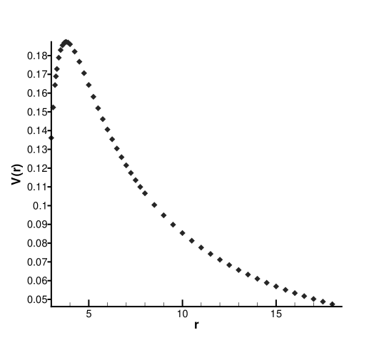
Figure 1: Brane potential for $R_{6},\cdots,R_{9}=\sqrt{2\alpha^{\prime}}$, $f=10$ and $p=2$.

The potential therefore behaves in a similar way to the brane-anti-brane potential computed in BS . The potential (77) is finite at the critical value of $r$ (76) but then becomes complex, indicating inelastic modes are opening up. At the critical separation, the interbrane force diverges for $p<3$, becoming infinitely attractive. At this point, an open string mode running between the different branes becomes massless, as can be seen from the expansion in (75). Specifically one can view the potential as coming from a one loop open string diagram without any external strings, i.e., just the partition function as in (25) (although with a different GSO projection for the open strings stretching between the branes). The coefficients of the $1/t$ terms in the exponentials in (75) (including the $r^{2}$ term) are then just the masses of the open string states stretching between the branes. A mode analysis of these open strings confirms this expectation.

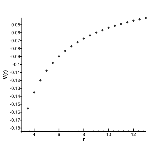
Figure 2: Brane potential for $R_{6},\cdots,R_{9}=\sqrt{\alpha^{\prime}/2}$, $f=1$ and $p=2$.

As the branes move closer together, a condensate of open string tachyons will form, accompanied by emission of closed string states. We expect the endpoint of this process to be a stable composite dyonic non-BPS brane, at a non-trivial minimum of the non-abelian open string tachyon. This kind of tachyon condensation has been considered before for a pair of electric non-BPS branes in lambertsachs , and from the supergravity point of view for a large number of coincident branes in gian .

The upshot of the small t expansion is that the potential must become attractive for $r$ near $r_{crit}$. Combined with the large t expansion we find that at the very least the potential must have an unstable equilibrium point for small enough values of $f$.

To investigate the potential further we performed the integration numerically using 500 digit precision arithmetic. We plot in figures 1,2 the two generic cases that we find for the potential. Specifically for the parameters in figure 1 $f<f_{crit}$, so that the potential is asymptotically repulsive, we find a local maximum in the potential at some separation of the branes and then an attractive potential for all smaller separations. In figure 2 we instead choose parameters such that $f>f_{crit}$ and find that the potential is attractive at all separations.

Finally, let us consider how one might generalize the brane configuration to realize a potential with a local minimum. For purely electric branes, the potential is a monotonic function of the separation, which is repulsive when the individual branes are tachyon-free. By introducing the lower dimensional brane charge we introduce a new length scale into the interbrane potential proportional to the string length times a function of the ratio of the charges. As we have seen this is sufficient to generate a local maximum in the potential. However the extra charge dominates the behavior at short distances, leading to a short-range attractive force. By introducing additional brane charges we introduce additional length scales into the interbrane potential and in general a local minimum should be present. A challenge for the future is to construct stable non-BPS brane solutions with these extra charges, which promise new insights into the brane world scenario.

- (1) N. Arkani-Hamed, S. Dimopoulos and G. Dvali, The hierarchy problem and new dimensions at a millimeter, Phys. Lett. B 429, 263 (1998) [hep-ph/9803315]; I. Antoniadis, N. Arkani-Hamed, S. Dimopoulos and G. Dvali, New dimensions at a millimeter to a Fermi and superstrings at a TeV, Phys. Lett. B 436, 257 (1998) [hep-ph/9804398].
- (2) Z. Kakushadze and S. H. Tye, Brane world, Nucl. Phys. B548, 180 (1999) [hep-th/9809147]; For a review, see for example, V. A. Rubakov, Large and infinite extra dimensions: An Introduction, hep-ph/0104152.
- (3) I. Antoniadis, String and D-brane physics at low energy, hep-th/0102202; A. Sagnotti, Open-string models with broken supersymmetry, Nucl. Phys. bf 88 Proc. Suppl. 160 (2000) [hep-th/0001077]; E. Dudas, Theory and phenomenology of type I strings and M-theory, Class. Quant. Grav. 17, R41 (2000) [hep-ph/0006190].
- (4) G. Aldazabal, L. E. Ibanez and F. Quevedo, On realistic brane worlds from type I strings, hep-ph/0005033.
- (5) A. Sen, Stable non-BPS states in string theory, J. High Energy Phys. 9806, 007 (1998) [hep-th/9803194].
- (6) N. Arkani-Hamed, S. Dimopoulos and J. March-Russell, Stabilization of sub-millimeter dimensions: The new guise of the hierarchy problem, Phys. Rev. D632001064020 [hep-th/9809124].
- (7) S. Corley and D. A. Lowe, Solving the hierarchy problem with brane crystals, Phys. Lett. B 505, 197 (2001) [hep-ph/0101021].
- (8) A. Sen, Stable non-BPS bound states of BPS D-branes, J. High Energy Phys. 9808, 010 (1998) [hep-th/9805019]; O. Bergman and M.R. Gaberdiel, Stable non-BPS D Particles, Phys. Lett. B 441, 133 (1998) [hep-th/9806155].
- (9) A. Sen, Non-BPS States and Branes in String Theory, hep-th/9904207.
- (10) M. Frau, L. Gallot, A. Lerda and P. Strigazzi Stable non-BPS D-branes in type I string theory, Nucl. Phys. B564, 60 (2000), [hep-th/9903123].
- (11) N. D. Lambert and I. Sachs, Non-abelian field theory of stable non-BPS branes, J. High Energy Phys. 0003, 028 (2000) [hep-th/0002061]; String loop corrections to stable non-BPS branes, J. High Energy Phys. 0102, 018 (2001) [hep-th/0010045].
- (12) G. L. Alberghi, E. Caceres, K. Goldstein and D. A. Lowe, Stacking non-BPS D-branes, hep-th/0105205.
- (13) M. R. Gaberdiel, Lectures on non-BPS Dirichlet branes, Class. Quant. Grav. 17, 3483 (2000) [hep-th/0005029].
- (14) P. Di Vecchia and A. Liccardo D-branes in String Theory, I, hep-th/9912161.
- (15) P. Di Vecchia and A. Liccardo D-branes in String Theory, II., hep-th/9912275.
- (16) A. Lerda and R. Russo Stable non-BPS states in string theory: a pedagogical review, Int. J. Mod. Phys. A15 (2000) 771, [hep-th/9905006].
- (17) A. Abouelsaood, C.G. Callan, C.R. Nappi, and S.A. Yost, Open Strings in Background Gauge Fields, Nucl. Phys. B280, 599 (1987).
- (18) J. Polchinski, String Theory (Cambridge University Press, 1998).
- (19) C.G. Callan, C. Lovelace, C.R. Nappi and S.A. Yost, Adding Holes and Crosscaps to the Superstring, Nucl. Phys. B293, 83 (1987).
- (20) J. Polchinski and Y. Cai Consistency of Open Superstring Theories, Nucl. Phys. B296, 91 (1988).
- (21) M.R. Gaberdiel and A. Sen, Non-supersymmetric D-brane Configurations with Bose-Fermi Degenerate Open String Spectrum, J. High Energy Phys. 9911, 008 (1999), [hep-th/9908060].
- (22) P. Di Vecchia, M. Frau, A. Lerda, A. Liccardo (F,Dp) bound states from the boundary state, Nucl. Phys. B565, 397 (2000), [hep-th/9906214].
- (23) H. Arfaei and D. Kamani Branes with Background Fields in Boundary State Formalism, Phys. Lett. B 452, 54 (1999), [hep-th/9909167].
- (24) D. Kamani Mixed Branes at Angle in Compact Spacetime, Phys. Lett. B 475, 39 (2000), [hep-th/9909079].
- (25) E. Eyras and S. Panda The Space-Time Life of a Non-BPS D-Particle, Nucl. Phys. B584, 251 (2000), [hep-th/0003033].
- (26) M. Billo, P. Di Vecchia, M. Frau, A. Lerda, I. Pesando, R. Russo and S. Sciuto, Microscopic string analysis of the D0-D8 brane system and dual R-R states, Nucl. Phys. B526, 199 (1998) [hep-th/9802088].
- (27) L. Gallot, A. Lerda and P. Strigazzi Gauge and gravitational interactions of non-BPS D-particles, Nucl. Phys. B586, 206 (2000), [hep-th/0001049].
- (28) T. Banks and L. Susskind Brane-Anti-Brane Forces, hep-th/9511194.