Quantum Energies of Solitons

Abstract

For renormalizable models a method is presented to unambiguously compute the energy that is carried by localized field configurations (solitons). A variational approach for the total energy is utilized to search for soliton configurations. As an example a $1+1$ dimensional model is considered. The quantum energy of configurations that are translationally invariant for a subset of coordinates is discussed.

In this talk I present results that emerged from the collaboration[1, 2, 3] with E. Farhi, N. Graham, R. L. Jaffe and M. Quandt.

1 Introduction

Field theories can contain spatially varying (but time independent) configurations $\Phi$ that are local minima of the classical energy. When quantum effects are taken into account, the classical description must be re–examined because the spatially varying soliton configuration should minimize the total energy

$$E_{\rm tot}[\Phi]=E_{\rm cl}[\Phi]+E_{\rm qu}[\Phi]$$ (1)

which takes into account classical ($E_{\rm cl}$) and quantum ($E_{\rm qu}$) contributions. Since the total energy for general configurations is difficult to compute, quantum effects are typically computed as approximate corrections to the classical soliton. In this talk I describe an approach that unambiguously yields the total energy up to one loop order, i.e. ${\cal O}(\hbar)$.

At ${\cal O}(\hbar)$ the quantum contribution is the sum of the change of the vacuum energy and the (local) counterterm functional

$$E_{\rm qu}[\Phi]=E_{\rm vac}[\Phi]+E_{\rm c.t.}[\Phi]\,.$$ (2)

Formally $E_{\rm vac}$ is given as the sum of the changes of the frequencies $\omega$ of the small amplitude fluctuations $\eta$ about $\Phi$. These frequencies are determined from a Schrödinger–type wave–equation

$$\left\{-\vec{\partial}\,^{2}+m^{2}+U(\Phi)\right\}\eta=\omega^{2}\eta\,,$$ (3)

with a potential $U$ that is obtained from $\Phi$. The evaluation of $E_{\rm vac}$ is non–perturbative as can e.g. be observed from the appearance of bound states in Eq. (3). $E_{\rm vac}$ is ultra–violet divergent and requires regularization. On the other hand, $E_{\rm c.t.}$ is computed as a local integral of $\Phi$ (and derivatives thereof) that contains divergent coefficients. Commonly these coefficients are determined in the perturbative sector (where $\Phi$ is set to its vacuum value) using e.g. dimensional regularization. The main problem is to find a regularization scheme for $E_{\rm vac}$ that is compatible with the determination of the counterterms such that the sum (2) is finite and unique for any prescribed background $\Phi$.

2 The Phase Shift Approach

The vacuum energy acquires contributions from states that are bound in the potential $U(\Phi)$ as well as from scattering states. While the former contribution can be expressed as a finite sum over discrete levels the latter may be computed from the change of the density of states. This change is given in terms of the derivative of the phases shifts $\delta(k)$. Thus I may formally write

$$E_{\rm vac}\,\sim\,\frac{1}{2}\sum_{i}^{\rm b.s.}|\omega_{i}|+\int_{0}^{\infty}\frac{dk}{2\pi}\omega_{k}\,\frac{d}{dk}\sum_{\ell}D_{\ell}\delta_{\ell}(k)\,,$$ (4)

where $\omega_{i}$ are the eigen–frequencies of the bound states and $D_{\ell}$ is the degeneracy factor associated with the channels labeled by $\ell$ (e.g. $D_{\ell}=2\ell+1$ if $\ell$ refers to orbital angular momentum). Furthermore $\omega_{k}=\sqrt{k^{2}+m^{2}}$. As already noted, the above integral is ultra–violet divergent. Fortunately the large $k$ behavior of the phase shifts can be isolated using the Born–series. This series represents an expansion of the phase shifts in terms of the potential $U$. In general this expansion does not converge for all $k$, however, it does for large enough $k$. The expansion of the vacuum energy in terms of $U$ can also be obtained from the expansion of ${\rm ln}\,{\rm det}(-\vec{\partial}\,^{2}+m^{2}+U)$ that corresponds to the evaluation of a set of Feynman diagrams. The identity of these expansions has been established utilizing dimensional regularization[1, 2]. Now the central idea[4, 5, 1] is to add and subtract the expansion in $U=U(\Phi)$. This yields

$$E_{\rm qu} = \sum_{i}^{\rm b.s.}\left|\frac{\omega_{i}}{2}\right|+\int_{0}^{\infty}\frac{dk}{2\pi}\,\omega_{k}\,\frac{d}{dk}\sum_{\ell}D_{\ell}\left\{\delta_{\ell}(k)-\delta^{(1)}_{\ell}(k)-\delta^{(2)}_{\ell}(k)-\ldots\right\}$$ (5)

$$\hskip 71.13188pt+\quad\begin{minipage}{142.26378pt} \psfig{} \end{minipage}+\ldots\,+E_{\rm c.t.},$$

where $U=U(\Phi)$ denotes the potential generated by the background field. The divergent Feynman diagrams in Eq. (5) can be computed using standard techniques and, when added to the counterterm contribution $E_{\rm c.t.}$, a finite and unique result for the total energy is obtained.

3 Chiral Model in D=1+1 as an Example

Now I would like to apply this formalism to a simple chiral model in $D=1+1$. In this model a two–component boson field $\vec{\phi}=(\phi_{1},\phi_{2})$ couples chirally to a fermion $\Psi$ that come in $N_{f}$ (equivalent) modes:

$${\cal L}=\frac{1}{2}\,\partial_{\mu}\vec{\phi}\cdot\partial^{\mu}\vec{\phi}+\sum_{n=1}^{N_{f}}\bar{\Psi}_{i}\left\{i\partial\hskip-5.0pt/-G\left(\phi_{1}+i\gamma_{5}\phi_{2}\right)\right\}\Psi_{i}\,.$$ (6)

where the potential for the boson field

$$V(\vec{\phi})=\frac{\lambda}{8}\left[\vec{\phi}\cdot\vec{\phi}-v^{2}+\frac{2\alpha v^{2}}{\lambda}\right]^{2}-\alpha v^{3}\left(\phi_{1}-v\right)+{\rm const.}\,$$ (7)

contains a term (proportional to $\alpha$) that breaks the chiral symmetry explicitly in order to avoid problems stemming from (unphysical) infra–red singularities that occur when the vacuum configuration would be determined via the naïve treatment of spontaneous symmetry breaking[6]. In this manner it is guaranteed that the VEV is given by $\langle\vec{\phi}\rangle=(v,0)$. Here the counterterm Lagrangian is not presented explicitly. It is determined such that the quantum corrections lead to a vanishing tadpole diagram for the boson field. Note that considering only the classical contribution does not support a stable soliton soliton.

In the limit that the number of fermion modes becomes large with $v^{2}/N_{f}\sim{\cal O}(1)$ only the classical and one fermion loop pieces contribute. In the following I will only consider that limit, i.e. $E_{\rm tot}=E_{\rm cl}+E_{\rm F}$. The fermion contribution can be split into two pieces $E_{\rm F}=E_{\rm vac}+E_{\rm val}$. The valence part $E_{\rm val}$ is given in terms of the bound state energies such as to saturate the total fermion number that is fixed to be $N_{F}$. The vacuum piece is computed according to the formalism described in the preceding section:

$$E_{\rm vac}=-\frac{1}{2}\sum_{i}^{\rm b.s.}\left(\left|\omega_{i}\right|-Gv\right)-\int_{0}^{\infty}\frac{dk}{2\pi}\,\left(\omega_{k}-Gv\right)\frac{d}{dk}\left(\delta_{\rm F}(k)-\delta^{(1)}(k)\right)\,,$$ (8)

which is obtained from Eq (5) by employing Levinson’s theorem. Here $\delta_{\rm F}$ denotes the sum of the eigenphase shifts. The subtraction

$$\delta^{(1)}(k)=\frac{2G^{2}}{k}\int_{0}^{\infty}dx\left(v^{2}-\vec{\phi}\,^{2}(x)\right)$$ (9)

that renders $E_{\rm vac}$ finite contains both first and second order Born approximants in the fluctuations of $\vec{\phi}$ about $\langle\vec{\phi}\rangle$. The first order is unambiguously fixed by the no–tadpole renormalization condition and the second order by the chiral symmetry.

Having established the energy functional I now consider variational Ansätze for the background field that turn this functional in a function of the variational parameters. As an example I assume

$$\phi_{1}+i\phi_{2}=v\left\{1-R+R\,{\rm exp}\hskip 0.28453pt\left[i\pi\left(1+{\rm tanh}(Gvx/w)\right)\right]\right\}$$ (10)

that introduces width ($w$) and amplitude ($R$) parameters. For prescribed model parameters ($G$,$v$,etc.) the energy must be minimized with respect to $w$ and $R$. The resulting binding energy $\epsilon_{\rm B}=E_{\rm tot}-Gv$ is shown in figure 1.

         

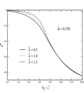
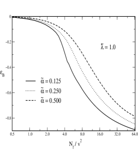
Figure 1: The maximal binding energy as a function of the model parameters as obtained from the Ansatz (10) in units of $Gv$; $\tilde{\alpha}={\alpha}/{G^{2}}$ and $\tilde{\lambda}={\lambda}/{G^{2}}$.

Even though the Ansatz (10) may not be the final answer to the minimalization problem, $\epsilon_{\rm B}$ is definitely negative. Thus a solitonic configuration is energetically favored showing that indeed quantum fluctuations can create a soliton that is not stable at the classical level.

4 Quantum Energies of Interfaces

In some cases (e.g. domain walls) the background potential in the Schrödinger–type equation depends only on a subset of the coordinates $U(x,\vec{y})=u(x)$, where the number of “trivial” dimensions is $n$: $\vec{y}=(y_{1},\ldots,y_{n})$. I will refer to such configurations as interfaces. The single particle energies then parametrically depend on the momentum $\vec{p}$ conjugate to $\vec{y}$: $\omega(p,k)=\sqrt{\vec{p}\,^{2}+m^{2}+k^{2}}$ and $\omega_{i}(p)=\sqrt{\vec{p}\,^{2}+m^{2}-\kappa_{i}^{2}}$, where $k$ and $\kappa_{i}$ label the scattering and bound states obtained from the one–dimensional Schrödinger–type equation for $u(x)$. However, the phase shifts depend only on the momentum $k$ conjugate to $x$: $\delta=\delta(k)$. When straightforwardly integrating the $n+1$ dimensional generalization of eq (5) over $\vec{p}$ a logarithmic singularity seems to emerge at $n=1$ because $\omega(p,k)-\sqrt{\vec{p}\,^{2}+m^{2}}\to k^{2}/2|\vec{p}|$ for large $|\vec{p}|$. This cannot be regularized by Born–subtractions that only involve $k$. As in dimensional regularization it is suitable to consider $n<1$. Other cases are obtained by analytic continuation. This yields the quantum energy (density) of the interface:

$$\epsilon(n) = -\frac{\Gamma\left(-\frac{n+1}{2}\right)}{(4\pi)^{\frac{n+1}{2}}}\left\{\int_{0}^{\infty}\frac{dk}{\pi}\left(\omega_{k}^{n+1}-m^{n+1}\right)\frac{d}{dk}\bar{\delta}(k)+\sum_{i}^{\rm b.s.}\left(\omega_{i}^{n+1}-m^{n+1}\right)\right\}$$ (11)

$$\hskip 56.9055pt+\epsilon_{\rm F.D.}+\epsilon_{\rm c.t.}$$

where $\bar{\delta}(k)$ denote the Born–subtracted phase shift and $\epsilon_{\rm F.D.}$ is the Feynman diagram contribution. While the known formulae, e.g. Eq (8) are recovered for $n=0$, the singularity for $n\to 1$ is reflected as a pole in the $\Gamma$ function. Consistency conditions require $\epsilon(1)$ to be finite. Hence the residuum of the pole in the $\Gamma$–function must vanish, i.e.

$$\int_{0}^{\infty}\frac{dk}{\pi}k^{2}\frac{d}{dk}\bar{\delta}(k)-\sum_{i}^{\rm b.s.}\kappa_{i}^{2}=0\,.$$ (12)

In this way a number of sum rules between bound state energies $\sqrt{m^{2}-\kappa_{i}^{2}}$ and (Born–subtracted) phase shifts can be established. Ultimately the limit $n\to 1$ can safely be assumed yielding the interface energy

$$\lim_{n\to 1}\epsilon(n) = -\frac{1}{4\pi}\left\{\int_{0}^{\infty}\frac{dk}{\pi}\left(\omega(k)^{2}\log\frac{\omega(k)^{2}}{4\pi\mu^{2}}-m^{2}\log\frac{m^{2}}{4\pi\mu^{2}}\right)\frac{d}{dk}\bar{\delta}(k)\right.\hskip 28.45274pt$$ (13)

$$\hskip 28.45274pt\left.+\sum_{i}\left(\omega_{i}^{2}\log\frac{\omega_{i}^{2}}{4\pi\mu^{2}}-m^{2}\log\frac{m^{2}}{4\pi\mu^{2}}\right)\right\}+\epsilon_{\rm F.D.}+\epsilon_{\rm c.t.}$$

The scale $\mu$ has been introduced for dimensional reasons. It is arbitrary because its contribution is proportional to the residuum (12).

5 Summary

In this talk I have presented a formalism to unambiguously and numerically feasibly compute the one–loop quantum corrections to energies of spatially varying field configurations. This approach strongly relies on the identity of Feynman diagrams and Born approximants to Casimir energies. Utilizing a variational approach to the total energy solitons can be constructed. As an example I have shown that in a $1+1$ dimensional chiral model quantum corrections create a soliton that is classically unstable. Finally I have derived a master formula for interface energies whose consistency demands sum rules for scattering data that can be considered generalizations of Levinson’s Theorem.

References

- [1] E. Farhi, N. Graham, R. L. Jaffe and H. Weigel, Phys. Lett. B 475 (2000) 335 [hep-th/9912283]; E. Farhi, N. Graham, R. L. Jaffe and H. Weigel, Nucl. Phys. B 585 (2000) 443 [hep-th/0003144].
- [2] E. Farhi, N. Graham, R. L. Jaffe and H. Weigel, Nucl. Phys. B 595 (2001) 536 [hep-th/0007189].
- [3] N. Graham, R. L. Jaffe, M. Quandt and H. Weigel, hep-th/0103010, Phys. Rev. Lett., in print; N. Graham, R. L. Jaffe, M. Quandt and H. Weigel, quant-ph/0104136, Ann. Phys., in print;
- [4] E. Farhi, N. Graham, P. Haagensen and R. L. Jaffe, Phys. Lett. B 427 (1998) 334 [hep-th/9802015].
- [5] J. Schwinger, Phys. Rev. 94 (1954) 1362; J. Baacke, Z. Phys. C 53 (1992) 402.
- [6] S. Coleman, Commun. Math. Phys. 31 (1973) 259.
- [7] R. D. Puff, Phys. Rev. A11 (1975) 154.