Gauge Field Theory Coherent States (GCS) : II.
Peakedness Properties

Abstract

In this article we apply the methods outlined in the previous paper of this series to the particular set of states obtained by choosing the complexifier to be a Laplace operator for each edge of a graph. The corresponding coherent state transform was introduced by Hall for one edge and generalized by Ashtekar, Lewandowski, Marolf, Mourão and Thiemann to arbitrary, finite, piecewise analytic graphs.

However, both of these works were incomplete with respect to the following two issues :
(a) The focus was on the unitarity of the transform and left the properties of the corresponding coherent states themselves untouched.
(b) While these states depend in some sense on complexified connections, it remained unclear what the complexification was in terms of the coordinates of the underlying real phase space.

In this paper we complement these results : First, we explicitly derive the complexification of the configuration space underlying these heat kernel coherent states and, secondly, prove that this family of states satisfies all the usual properties :
i) Peakedness in the configuration, momentum and phase space (or Bargmann-Segal) representation.
ii) Saturation of the unquenched Heisenberg uncertainty bound.
iii) (Over)completeness.

These states therefore comprise a candidate family for the semi-classical analysis of canonical quantum gravity and quantum gauge theory coupled to quantum gravity. They also enable error-controlled approximations to difficult analytical calculations and therefore set a new starting point for numerical canonical quantum general relativity and gauge theory.

The text is supplemented by an appendix which contains extensive graphics in order to give a feeling for the so far unknown peakedness properties of the states constructed.

1 Introduction

Quantum General Relativity (QGR) has matured over the past decade to a mathematically well-defined theory of quantum gravity. In contrast to string theory, by definition QGR is a manifestly background independent, diffeomorphism invariant and non-perturbative theory. The obvious advantage is that one will never have to postulate the existence of a non-perturbative extension of the theory, which in string theory has been called the still unknown M(ystery)-Theory.

The disadvantage of a non-perturbative and background independent formulation is, of course, that one is faced with new and interesting mathematical problems so that one cannot just go ahead and “start calculating scattering amplitudes”: As there is no background around which one could perturb, rather the full metric is fluctuating, one is not doing quantum field theory on a spacetime but only on a differential manifold. Once there is no (Minkowski) metric at our disposal, one loses familiar notions such as causality structure, locality, Poincaré group and so forth, in other words, the theory is not a theory to which the Wightman axioms apply. Therefore, one must build an entirely new mathematical apparatus to treat the resulting quantum field theory which is drastically different from the Fock space picture to which particle physicists are used to.

As a consequence, the mathematical formulation of the theory was the main focus of research in the field over the past decade. The main achievements to date are the following (more or less in chronological order) :

• Kinematical Framework
  The starting point was the introduction of new field variables [2] for the gravitational field which are better suited to a background independent formulation of the quantum theory than the ones employed until that time. In its original version these variables were complex valued, however, currently their real valued version, considered first in [3] for classical Euclidean gravity and later in [4] for classical Lorentzian gravity, is preferred because to date it seems that it is only with these variables that one can rigorously define the kinematics and dynamics of Euclidean or Lorentzian quantum gravity [5].
  These variables are coordinates for the infinite dimensional phase space of an $SU(2)$ gauge theory subject to further constraints besides the Gauss law, that is, a connection and a canonically conjugate electric field. As such, it is very natural to introduce smeared functions of these variables, specifically Wilson loop and electric flux functions. (Notice that one does not need a metric to define these functions, that is, they are background independent). This had been done for ordinary gauge fields already before in [6] and was then reconsidered for gravity (see e.g. [7]).
  The next step was the choice of a representation of the canonical commutation relations between the electric and magnetic degrees of freedom. This involves the choice of a suitable space of distributional connections [8] and a faithful measure thereon [9] which, as one can show [10], is $\sigma$-additive. The proof that the resulting Hilbert space indeed solves the adjointness relations induced by the reality structure of the classical theory as well as the canonical commutation relations induced by the symplectic structure of the classical theory can be found in [11]. Independently, a second representation of the canonical commutation relations, called the loop representation, had been advocated (see e.g. [12] and especially [13] and references therein) but both representations were shown to be unitarily equivalent in [14] (see also [15] for a different method of proof).
  This is then the first major achievement : The theory is based on a rigorously defined kinematical framework.

• Geometrical Operators
  The second major achievement concerns the spectra of positive semi-definite, self-adjoint geometrical operators measuring lengths [16], areas [17, 18] and volumes [17, 19, 20, 21, 12] of curves, surfaces and regions in spacetime. These spectra are pure point (discete) and imply a discrete Planck scale structure. It should be pointed out that the discreteness is, in contrast to other approaches to quantum gravity, not put in by hand but it is a prediction !

• Regularization- and Renormalization Techniques
  The third major achievement is that there is a new regularization and renormalization technique [22, 23] for diffeomorphism covariant, density-one-valued operators at our disposal which was successfully tested in model theories [24]. This technique can be applied, in particular, to the standard model coupled to gravity [25, 26] and to the Poincaré generators at spatial infinity [27]. In particular, it works for Lorentzian gravity while all earlier proposals could at best work in the Euclidean context only (see, e.g. [13] and references therein). The algebra of important operators of the resulting quantum field theories was shown to be consistent [28]. Most surprisingly, these operators are UV and IR finite ! Notice that, at least as far as these operators are concerned, this result is stronger than the believed but unproved finiteness of scattering amplitudes order by order in perturbation theory of the five critical string theories, in a sense we claim that the perturbation series converges. The absence of the divergences that usually plague interacting quantum fields propagating on a Minkowski background can be understood intuitively from the diffeomorphism invariance of the theory : “short and long distances are gauge equivalent”. We will elaborate more on this point in future publications.

• Spin Foam Models
  After the construction of the densely defined Hamiltonian constraint operator of [22, 23], a formal, Euclidean functional integral was constructed in [29] and gave rise to the so-called spin foam models (a spin foam is a history of a graph with faces as the history of edges) [30]. Spin foam models are in close connection with causal spin-network evolutions [31], state sum models [32] and topological quantum field theory, in particular BF theory [33]. To date most results are at a formal level and for the Euclidean version of the theory only but the programme is exciting since it may restore manifest four-dimensional diffeomorphism invariance which in the Hamiltonian formulation is somewhat hidden.

• Finally, the fifth major achievement is the existence of a rigorous and satisfactory framework [34, 35, 36, 37, 38, 39, 40] for the quantum statistical description of black holes which reproduces the Bekenstein-Hawking Entropy-Area relation and applies, in particular, to physical Schwarzschild black holes while stringy black holes so far are under control only for extremal charged black holes.

Summarizing, the work of the past decade has now culminated in a promising starting point for a quantum theory of the gravitational field plus matter and the stage is set to pose and answer physical questions.

The most basic and most important question that one should ask is : Does the theory have classical general relativity as its classical limit ? Notice that even if the answer is negative, the existence of a consistent, interacting, diffeomorphism invariant quantum field theory in four dimensions is already a quite non-trivial result. However, we can claim to have a satisfactory quantum theory of Einstein’s theory only if the answer is positive.

It seems that the most natural framework for deriving the classical limit of a theory is based on coherent states or best approximation states. Coherent states have a long history and an extensive literature exists in a vast range of applications (see e.g. [41, 42] and references therein). It has been pointed out by many (see e.g. [43]) that they are best suited for the analysis of the semi-classical behaviour of any given system because, among other things, in contrast to the WKB-methods more familiar to physicists they avoid the discussion of the critical turning points and it is much more natural to ask questions which address regions in the classical phase space rather than in configuration and momentum space only.

Surprisingly, the vast majority of coherent states have been constructed for systems with only a finite number of degrees of freedom. This is astonishing because in the course of constructions of (interacting) quantum field theories from given classical ones one is almost always forced to regularize and renormalize the operators in that theory and these are operations which have no classical counterpart. Thus, it would be no surprise if it turned out that the classical limit of such quantum field theories is not the classical field theory that one started from. Just to give an example, even if one could rigorously show that the continuum limit of lattice QCD exists, to the best of the knowledge of the authors it is at present unclear whether the classical limit of that continuum quantum field theory would give us back classical $SU(3)$ Yang-Mills theory coupled to quarks.

This paper is the second one in a series of papers [46, 47, 48, 49, 50, 51] entitled “Gauge Field Theory Coherent States” which are geared at shedding light at these questions. Specifically, we are interested in the question whether the non-perturbative quantization of continuum Lorentzian general relativity in four dimensions with and without matter advertized in [22, 23, 25] has the correct classical limit. In fact we eliminate the criticism stated in [44] and show in [45] that quantum general relativity as presently formulated does admit graviton states which would then presumably also enable us to make contact with results from perturbation theory.

The general outline of our programme was given in [46] where a huge family of coherent states, based on the phase space complexifier method [52], was introduced. Here we specialize to the “heat kernel family” of coherent states that results by choosing the square of electric flux variables as the complexifier which, upon quantization, becomes a Laplacian. This choice is motivated, on the one hand by the beautiful analysis of Hall [53, 54] who established a unitary transfomation between square integrable functions on a compact gauge group with respect to the Haar measure and square integrable, holomorphic functions on the complexified group with respect to the so-called heat kernel measure. On the other hand, it is convenient since an application of this framework to diffeomorphism invariant gauge theories hs already been started in in [55].

The original purpose of [55] was to solve the reality conditions of quantum general relativity written in terms of the complex valued Ashtekar connection and therefore the properties of the states that came with that heat kernel transform remained untouched. Moreover, the heat kernel transform of [55] obviously complexifies the real connection but it remained unclear how that complex valued connection is expressed in terms of the coordinates of the real phase space. Without that knowledge there is obviously no interpretation of that complex valued connection possible. In this paper we will fill both of these gaps. Namely, using the classical framework of [56] and the complexifier method of [52] we explicitly construct the complex connection out of the real phase space variables. Secondly, we analyze in detail the semi-classical properties of the coherent states so obtained, most importantly their peakedness properties.

This we do in great detail for the compact gauge groups of rank one, that is, $U(1)$ and $SU(2)$, and sketch how the proofs extend to compact groups of higher rank. Details will appear in the forthcoming paper [57]. Coherent states for Higgs fields are completely analogous to the coherent states constructed here because one can describe them by so-called “point-holonomies” [26] which are a special case of the holonomies considered here. Details and coherent states for fermions are treated in [49].

As it will become obvious, the states constructed in this paper can serve as a tool to perform error-controlled rigorous approximations in quantum general relativity and quantum gauge theory coupled to quantum gravity and therefore as a starting point for numerical canonical quantum general relativity and numerical canonical quantum gauge theory coupled to quantum gravity.

The present article is organized as follows :

Section two is an account of the relevant notions and techniques of non-perturbative classical and quantum general relativity.

Section three explicitly derives the particular complexification of the real phase space of gauge theories or real general relativity based on heat kernel generators as complexifiers. This section depends on the recently constructed theory of symplectic manifolds of quantum general relativity and quantum gauge theory labelled by graphs [56].

Section four introduces the heat kernel family of gauge-non-invariant states for a general gauge theory without fermions in any spacetime dimension and we prove that they satisfy all the properties that one is used to from the classical harmonic oscillator coherent states. That is, these states are labelled by a classical connection and a classical electric field (a point in phase space) and we show that these states are peaked on these values in the connection-, momentum- and Segal-Bargmann representation. Furthermore, we show that the system of states is overcomplete, saturates the unquenched Heisenberg uncertainty bound with respect to certain complexified holonomy operators and that each state labelled by a point in phase space can be associated with a phase space cell with a volume whose size is controlled by $\hbar^{d}$. We do all this for the gauge group $SU(2)$ and point out how to generalize to an arbitrary compact gauge group.

In section five the analysis of section four 3 is generalized to the gauge invariant heat kernel family. The proofs follow essentially from the proofs derived in section four by employing the group averaging method of refined algebraic quantization (RAQ) [11]. However, the results stated in section five are somewhat less complete than those for section four due to the difficulty to do the group averaging explicitly which makes it hard to establish sharp peakedness. Fortunately, the results of section four are completely sufficient in order to study the semi-classical behaviour of the theory.

Finally in Appendix A we repeat our analysis for the technically much simpler case of $G=U(1)$ and in Appendix B we display the peakedness properties of the states constructed in the configuration and Bargmann-Segal representation graphically, both for $SU(2)$ and $U(1)$. All graphics have been obtained by means of Mathematica and the admittedly large amount of plots is justified by the fact that, to the best of our knowledge, the behaviour of these states has not been studied numerically before.

2 Kinematical Structure of Diffeomorphism Invariant Quantum Gauge Theories

In this section we will recall the main ingredients of the mathematical formulation of (Lorentzian) diffeomorphism invariant classical and quantum field theories of connections with local degrees of freedom in any dimension and for any compact gauge group. See [56, 11] and references therein for more details. Also, in this section we will take all quantities to be dimensionless for simplicity, the incoporation of dimensionful parameters will be discussed in the next section.

2.1 Classical Theory

Let $G$ be a compact gauge group, $\Sigma$ a $D-$dimensional manifold admitting a principal $G-$bundle with connection over $\Sigma$. Let us denote the pull-back to $\Sigma$ of the connection by local sections by $A_{a}^{i}$ where $a,b,c,..=1,..,D$ denote tensorial indices and $i,j,k,..=1,..,\dim(G)$ denote indices for the Lie algebra of $G$. Likewise, consider a vector bundle of electric fields, whose projection to $\Sigma$ is a Lie algebra valued vector density of weight one. We will denote the set of generators of the rank $N-1$ Lie algebra of $G$ by $\tau_{i}$ which are normalized according to $\mbox{tr}(\tau_{i}\tau_{j})=-N\delta_{ij}$ and $[\tau_{i},\tau_{j}]=2f_{ij}\;^{k}\tau_{k}$ defines the structure constants of $Lie(G)$.

Let $F^{a}_{i}$ be a Lie algebra valued vector density test field of weight one and let $f_{a}^{i}$ be a Lie algebra valued covector test field. We consider the smeared quantities

$$F(A):=\int_{\Sigma}d^{D}xF^{a}_{i}A_{a}^{i}\mbox{ and }E(f):=\int_{\Sigma}d^{D}xE^{a}_{i}f_{a}^{i}$$ (2.1)

While both are diffeomorphism covariant, it is only the latter which is gauge covariant, one reason to consider the singular smearings discussed below. The choice of the space of pairs of test fields $(F,f)\in{\cal S}$ depends on the boundary conditions on the space of connections and electric fields which in turn depends on the topology of $\Sigma$ and will not be specified in what follows.

Consider the set $M$ of all pairs of smooth functions $(A,E)$ on $\Sigma$ such that (2.1) is well defined for any $(F,f)\in{\cal S}$. We define a topology on $M$ through the following globally defined metric :

$$d_{\rho,\sigma}[(A,E),(A^{\prime},E^{\prime})]$$

$$:= \sqrt{-\frac{1}{N}\int_{\Sigma}d^{D}x[\sqrt{\det(\rho)}\rho^{ab}\mbox{tr}([A_{a}-A^{\prime}_{a}][A_{b}-A^{\prime}_{b}])+\frac{[\sigma_{ab}\mbox{tr}([E^{a}-E^{a\prime}][E^{b}-E^{b\prime}])}{\sqrt{\det(\sigma)}}]}$$

where $\rho_{ab},\sigma_{ab}$ are fiducial metrics on $\Sigma$ of everywhere Euclidean signature. Their fall-off behaviour has to be suited to the boundary conditions of the fields $A,E$ at spatial infinity. Notice that the metric (2.1) on $M$ is gauge invariant. It can be used in the usual way to equip $M$ with the structure of a smooth, infinite dimensional differential manifold modelled on a Banach (in fact Hilbert) space $\cal E$ where ${\cal S}\times{\cal S}\subset{\cal E}$. (It is the weighted Sobolev space $H_{0,\rho}^{2}\times H_{0,\sigma^{-1}}^{2}$ in the notation of [58]).

Finally, we equip $M$ with the structure of an infinite dimensional symplectic manifold through the following strong (in the sense of [59]) symplectic structure

$$\Omega((f,F),(f^{\prime},F^{\prime}))_{m}:=\int_{\Sigma}d^{D}x[F^{a}_{i}f^{i\prime}_{a}-F^{a\prime}_{i}f_{a}^{i}](x)$$ (2.3)

for any $(f,F),(f^{\prime},F^{\prime})\in{\cal E}$. We have abused the notation by identifying the tangent space to $M$ at $m$ with $\cal E$. To prove that $\Omega$ is a strong symplectic structure one uses standard Banach space techniques. Computing the Hamiltonian vector fields (with respect to $\Omega$) of the functions $E(f),F(A)$ we obtain the following elementary Poisson brackets

$$\{E(f),E(f^{\prime})\}=\{F(A),F^{\prime}(A)\}=0,\;\{E(f),A(F)\}=F(f)$$ (2.4)

As a first step towards quantization of the symplectic manifold $(M,\Omega)$ one must choose a polarization. As usual in gauge theories, we will use connections as the configuration variables and electric fields as canonically conjugate momenta. As a second step one must decide on a complete set of coordinates of $M$ which are to become the elementary quantum operators. The analysis just outlined suggests to use the coordinates $E(f),F(A)$. However, the well-known immediate problem is that these coordinates are not gauge covariant. Thus, we proceed as follows :

Let $\Gamma^{\omega}_{0}$ be the set of all piecewise analytic, finite, oriented graphs $\gamma$ embedded into $\Sigma$ and denote by $E(\gamma)$ and $V(\gamma)$ respectively its sets of oriented edges $e$ and vertices $v$ respectively. Here finite means that $E(\gamma)$ is a finite set. (One can extend the framework to $\Gamma^{\infty}_{0}$, the restriction to webs of the set of piecewise smooth graphs [60, 61] but the description becomes more complicated and we refrain from doing this here). It is possible to consider the set $\Gamma^{\omega}_{\sigma}$ of piecewise analytic, infinite graphs with an additional regularity property [48] but for the purpose of this paper it will be sufficient to stick to $\Gamma^{\omega}_{0}$. The subscript ₀ as usual denotes “of compact support” while _σ denotes “$\sigma$-finite”.

We denote by $h_{e}(A)$ the holonomy of $A$ along $e$ and say that a function $f$ on ${\cal A}$ is cylindrical with respect to $\gamma$ if there exists a function $f_{\gamma}$ on $G^{|E(\gamma)|}$ such that $f=p_{\gamma}^{\ast}f_{\gamma}=f_{\gamma}\circ p_{\gamma}$ where $p_{\gamma}(A)=\{h_{e}(A)\}_{e\in E(\gamma)}$. Holonomies are invariant under reparameterizations of the edge and in this article we assume that the edges are always analyticity preserving diffeomorphic images from $[0,1]$ to a one-dimensional submanifold of $\Sigma$. Gauge transformations are functions $g:\;\Sigma\mapsto G;\;x\mapsto g(x)$ and they act on holonomies as $h_{e}\mapsto g(e(0))h_{e}g(e(1))^{-1}$.

Next, given a graph $\gamma$ we choose a polyhedronal decomposition $P_{\gamma}$ of $\Sigma$ dual to $\gamma$. The precise definition of a dual polyhedronal decomposition can be found in [56] but for the purposes of the present paper it is sufficient to know that $P_{\gamma}$ assigns to each edge $e$ of $\gamma$ an open “face” $S_{e}$ (a polyhedron of codimension one embedded into $\Sigma$) with the following properties :
(1) the surfaces $S_{e}$ are mutually non-intersecting,
(2) only the edge $e$ intersects $S_{e}$, the intersection is transversal and consists only of one point which is an interiour point of both $e$ and $S_{e}$,
(3) $S_{e}$ carries the orientation which agrees with the orientation of $e$.
Furthermore, we choose a system $\Pi_{\gamma}$ of paths $\rho_{e}(x)\subset S_{e},\;x\in S_{e},\;e\in E(\gamma)$ connecting the intersection point $p_{e}=e\cap S_{e}$ with $x$. The paths vary smoothly with $x$ and the triples $(\gamma,P_{\gamma},\Pi_{\gamma})$ have the property that if $\gamma,\gamma^{\prime}$ are diffeomorphic, so are $P_{\gamma},P_{\gamma^{\prime}}$ and $\Pi_{\gamma},\Pi_{\gamma^{\prime}}$.

With these structures we define the following function on $(M,\Omega)$

$$P^{e}_{i}(A,E):=-\frac{1}{N}\mbox{tr}(\tau_{i}h_{e}(0,1/2)[\int_{S_{e}}h_{\rho_{e}(x)}\ast E(x)h_{\rho_{e}(x)}^{-1}]h_{e}(0,1/2)^{-1})$$ (2.5)

where $h_{e}(s,t)$ denotes the holonomy of $A$ along $e$ between the parameter values $s<t$, $\ast$ denotes the Hodge dual, that is, $\ast E$ is a $(D-1)-$form on $\Sigma$, $E^{a}:=E^{a}_{i}\tau_{i}$ and we have chosen a parameterization of $e$ such that $p_{e}=e(1/2)$.

Notice that in contrast to similar variables used earlier in the literature the function $P^{e}_{i}$ is gauge covariant. Namely, under gauge transformations it transforms as $P^{e}\mapsto g(e(0))P^{e}g(e(0))^{-1}$, the price to pay being that $P^{e}$ depends on both $A$ and $E$ and not only on $E$. The idea is therefore to use the variables $h_{e},P^{e}_{i}$ for all possible graphs $\gamma$ as the coordinates of $M$.

The problem with the functions $h_{e}(A)$ and $P^{e}_{i}(A,E)$ on $M$ is that they are not differentiable on $M$, that is, $Dh_{e},DP^{e}_{i}$ are nowhere bounded operators on $\cal E$ as one can easily see. The reason for this is, of course, that these are functions on $M$ which are not properly smeared with functions from $\cal S$, rather they are smeared with distributional test functions with support on $e$ or $S_{e}$ respectively. Nevertheless one would like to base the quantization of the theory on these functions as basic variables because of their gauge and diffeomorphism covariance. Indeed, under diffeomorphisms $h_{e}\mapsto h_{\varphi^{-1}(e)},P^{e}_{j}\mapsto P^{\varphi^{-1}(e)}_{j}$ where we abuse notation since $P^{e}$ depends also explicitly on the $S_{e},\rho_{e}$, see [56] for details. We proceed as follows.

Definition 2.1

By $\bar{M}_{\gamma}$ we denote the direct product $[G\times Lie(G)]^{|E(\gamma)|}$. The subset of $\bar{M}_{\gamma}$ of pairs $(h_{e}(A),P^{e}_{i}(A,E))_{e\in E(\gamma)}$ as $(A,E)$ varies over $M$ will be denoted by $(\bar{M}_{\gamma})_{|M}$. We have a corresponding map $p_{\gamma}:\;M\mapsto\bar{M}_{\gamma}$ which maps $M$ onto $(\bar{M}_{\gamma})_{|M}$.

Notice that the set $(\bar{M}_{\gamma})_{|M}$ is in general a proper subset of $M_{\gamma}$, depending on the boundary conditions on $(A,E)$, the topology of $\Sigma$ and the “size” of $e,S_{e}$. For instance, in the limit of $e,S_{e}\to e\cap S_{e}$ but holding the number of edges fixed, $(\bar{M}_{\gamma})_{|M}$ will consist of only one point in $\bar{M}_{\gamma}$. This follows from the smoothness of the $(A,E)$.

We equip a subset $M_{\gamma}$ of $\bar{M}_{\gamma}$ with the structure of a differentiable manifold modelled on the Banach space ${\cal E}_{\gamma}={\mathchoice{\hbox{\hbox to0.0pt{\kern 3.53328pt\vrule height=7.37993pt\hss}\hbox{$\displaystyle\rm R$}}}{\hbox{\hbox to0.0pt{\kern 3.53328pt\vrule height=7.37993pt\hss}\hbox{$\textstyle\rm R$}}}{\hbox{\hbox to0.0pt{\kern 2.47328pt\vrule height=5.16595pt\hss}\hbox{$\scriptstyle\rm R$}}}{\hbox{\hbox to0.0pt{\kern 1.76663pt\vrule height=3.68996pt\hss}\hbox{$\scriptscriptstyle\rm R$}}}}^{2\dim(G)|E(\gamma)|}$ by using the natural direct product manifold structure of $[G\times Lie(G)]^{|E(\gamma)|}$. While $\bar{M}_{\gamma}$ is a kind of distributional phase space, $M_{\gamma}$ satisfies appropriate regularity properties similar to $M$.

In order to proceed and to give $M_{\gamma}$ a symplectic structure derived from $(M,\Omega)$ one must regularize the elementary functions $h_{e},P^{e}_{i}$ by writing them as limits (in which the regulator vanishes) of functions which can be expressed in terms of the $F(A),E(f)$. Then one can compute their Poisson brackets with respect to the symplectic structure $\Omega$ at finite regulator and then take the limit pointwise on $M$. The result is the following well-defined strong symplectic structure $\Omega_{\gamma}$ on $M_{\gamma}$.

$$\{h_{e},h_{e^{\prime}}\}_{\gamma} = 0$$

$$\{P^{e}_{i},h_{e^{\prime}}\}_{\gamma} = \delta^{e}_{e^{\prime}}\frac{\tau_{i}}{2}h_{e}$$

$$\{P^{e}_{i},P^{e^{\prime}}_{j}\}_{\gamma} = -\delta^{ee^{\prime}}f_{ij}\;^{k}P^{e}_{k}$$ (2.6)

Since $\Omega_{\gamma}$ is obviously block diagonal, each block standing for one copy of $G\times Lie(G)$, to check that $\Omega_{\gamma}$ is non-degenerate and closed reduces to doing it for each factor together with an appeal to well-known Hilbert space techniques to establish that $\Omega_{\gamma}$ is a surjection of ${\cal E}_{\gamma}$. This is done in [56] where it is shown that each copy is isomorphic with the cotangent bundle $T^{\ast}G$ equipped with the symplectic structure (2.1) (choose $e=e^{\prime}$ and delete the label $e$).

Now that we have managed to assign to each graph $\gamma$ a symplectic manifold $(M_{\gamma},\Omega_{\gamma})$ we can quantize it by using geometric quantization. This can be done in a well-defined way because the relations (2.1) show that the corresponding operators are non-distributional. This is therefore a clean starting point for the regularization of any operator of quantum gauge field theory which can always be written in terms of the $\hat{h}_{e},\hat{P}^{e},\;e\in E(\gamma)$ if we apply this operator to a function which depends only on the $h_{e},\;e\in E(\gamma)$.

As an example [56], recall that $(M_{\gamma},\Omega_{\gamma})$ is subject to a coisotropic constraint, the Gauss constraint, which in terms of the quantities defined above can be written

$$G(\Lambda)=\sum_{v\in V(\gamma)}\Lambda^{i}[\sum_{e\in E(\gamma),e(0)=v}P^{e}_{i}-\sum_{e\in E(\gamma),e(1)=v}O_{ij}(h_{e})P^{e}_{j}]$$ (2.7)

where the smooth, Lie-algebra valued function of rapid decrease $\Lambda$ is a test function on $\Sigma$ enforcing the local constraint

$$G_{i}(v)=\sum_{e\in E(\gamma),e(0)=v}P^{e}_{i}-\sum_{e\in E(\gamma),e(1)=v}O_{ij}(h_{e})P^{e}_{j}$$ (2.8)

where $O_{ij}(h)=-\mbox{tr}(h\tau_{i}h^{-1}\tau_{j})/N$. Since $G(\Lambda)$ is coisotropic, specifically

$$\{G(\Lambda),G(\Lambda^{\prime})\}=-G([\Lambda,\Lambda^{\prime}])$$ (2.9)

the dimension of the physical configuration space equals half the dimension of $M_{\gamma}$ (which is $E\dim(G)$) minus $V\dim(G)$, the number of constraints. The question is what $(M_{\gamma},\Omega_{\gamma})$ has to do with $M,\Omega$. In [56] it is shown that there exists a partial order $\prec$ on the set $\cal L$ of triples $l=(\gamma,P_{\gamma},\Pi_{\gamma})$. In particular, $\gamma\prec\gamma^{\prime}$ means $\gamma\subset\gamma^{\prime}$ and $\cal L$ is a directed set so that one can form a generalized projective limit $M_{\infty}$ of the $M_{\gamma}$ (we abuse notation in displaying the dependence of $M_{\gamma}$ on $\gamma$ only rather than on $l$). For this one verifies that the family of symplectic structures $\Omega_{\gamma}$ is self-consistent in the sense that if $(\gamma,P_{\gamma},\Pi_{\gamma})\prec(\gamma^{\prime},P_{\gamma^{\prime}},\Pi_{\gamma^{\prime}})$ then $p_{\gamma^{\prime}\gamma}^{\ast}\{f,g\}_{\gamma}=\{p_{\gamma^{\prime}\gamma}^{\ast}f,p_{\gamma^{\prime}\gamma}^{\ast}g\}_{\gamma^{\prime}}$ for any $f,g\in C^{\infty}(M_{\gamma})$ and $p_{\gamma^{\prime}\gamma}:\;M_{\gamma^{\prime}}\mapsto M_{\gamma}$ is a system of natural projections, more precisely, of (non-invertible) symplectomorphisms.

Now, via the maps $p_{\gamma}$ of definition 2.1 we can identify $M$ with a subset of $M_{\infty}$. Moreover, in [56] it is shown that there is a generalized projective sequence $(\gamma_{n},P_{\gamma_{n}},\Pi_{\gamma_{n}})$ such that $\lim_{n\to\infty}p_{\gamma_{n}}^{\ast}\Omega_{\gamma_{n}}=\Omega$ pointwise in $M$. This displays $(M,\Omega)$ as embedded into a generalized projective limit of the $(M_{\gamma},\Omega_{\gamma})$, intuitively speaking, as $\gamma$ fills all of $\Sigma$, we recover $(M,\Omega)$ from the $(M_{\gamma},\Omega_{\gamma})$. Of course, this works with $\Gamma^{\omega}_{0}$ only if $\Sigma$ is compact, otherwise we need the extension to $\Gamma^{\omega}_{\sigma}$.

It follows that quantization of $(M,\Omega)$, and conversely taking the classical limit, can be studied purely in terms of $(M_{\gamma},\Omega_{\gamma})$ for all $\gamma$. The quantum kinematical framework for this will be given in the next subsection.

2.2 Quantum Theory

Let us denote the set of all smooth connections by ${\cal A}$. This is our classical configuration space and we will choose for its coordinates the holonomies $h_{e}(A),\;e\in\gamma,\;\gamma\in\Gamma^{\omega}_{0}$. ${\cal A}$ is naturally equipped with a metric topology induced by (2.1).

Recall the notion of a function cylindrical over a graph from the previous subsection. A particularly useful set of cylindrical functions are the so-called spin-netwok functions [62, 63, 14]. A spin-network function is labelled by a graph $\gamma$, a set of non-trivial irreducible representations $\vec{\pi}=\{\pi_{e}\}_{e\in E(\gamma)}$ (choose from each equivalence class of equivalent representations once and for all a fixed representant), one for each edge of $\gamma$, and a set $\vec{c}=\{c_{v}\}_{v\in V(\gamma)}$ of contraction matrices, one for each vertex of $\gamma$, which contract the indices of the tensor product $\otimes_{e\in E(\gamma)}\pi_{e}(h_{e})$ in such a way that the resulting function is gauge invariant. We denote spin-network functions as $T_{I}$ where $I=\{\gamma,\vec{\pi},\vec{c}\}$ is a compound label. One can show that these functions are linearly independent. From now on we denote by $\tilde{\Phi}_{\gamma}$ finite linear combinations of spin-network functions over $\gamma$, by $\Phi_{\gamma}$ the finite linear combinations of elements from any possible $\tilde{\Phi}_{\gamma^{\prime}},\;\gamma^{\prime}\subset\gamma$ a subgraph of $\gamma$ and by $\Phi$ the finite linear combinations of spin-network functions over an arbitrary collection of graphs. Clearly $\tilde{\Phi}_{\gamma}$ is a subspace of $\Phi_{\gamma}$. To express this distinction we will say that functions in $\tilde{\Phi}_{\gamma}$ are labelled by the “coloured graphs” $\gamma$ while functions in $\Phi_{\gamma}$ are labelled simply by graphs $\gamma$ where we abuse notation by using the same symbol $\gamma$.

The set $\Phi$ of finite linear combinations of spin-network functions forms an Abelian ^∗ algebra of functions on ${\cal A}$. By completing it with respect to the sup-norm topology it becomes an Abelian C^∗ algebra $\cal B$ (here the compactness of $G$ is crucial). The spectrum ${\overline{\cal A}}$ of this algebra, that is, the set of all algebraic homomorphisms ${\cal B}\mapsto{\mathchoice{\hbox{\hbox to0.0pt{\kern 3.46661pt\vrule height=7.37993pt\hss}\hbox{$\displaystyle\rm C$}}}{\hbox{\hbox to0.0pt{\kern 3.46661pt\vrule height=7.37993pt\hss}\hbox{$\textstyle\rm C$}}}{\hbox{\hbox to0.0pt{\kern 2.42662pt\vrule height=5.16595pt\hss}\hbox{$\scriptstyle\rm C$}}}{\hbox{\hbox to0.0pt{\kern 1.7333pt\vrule height=3.68996pt\hss}\hbox{$\scriptscriptstyle\rm C$}}}}$ is called the quantum configuration space. This space is equipped with the Gel’fand topology, that is, the space of continuous functions $C^{0}({\overline{\cal A}})$ on ${\overline{\cal A}}$ is given by the Gel’fand transforms of elements of $\cal B$. Recall that the Gel’fand transform is given by $\tilde{f}(\bar{A}):=\bar{A}(f)\;\forall\bar{A}\in{\overline{\cal A}}$. It is a general result that ${\overline{\cal A}}$ with this topology is a compact Hausdorff space. Obviously, the elements of ${\cal A}$ are contained in ${\overline{\cal A}}$ and one can show that ${\cal A}$ is even dense [64]. Generic elements of ${\overline{\cal A}}$ are, however, distributional.

The idea is now to construct a Hilbert space consisting of square integrable functions on ${\overline{\cal A}}$ with respect to some measure $\mu$. Recall that one can define a measure on a locally compact Hausdorff space by prescribing a positive linear functional $\chi_{\mu}$ on the space of continuous functions thereon. The particular measure we choose is given by $\chi_{\mu_{0}}(\tilde{T}_{I})=1$ if $I=\{\{p\},\vec{0},\vec{1}\}$ and $\chi_{\mu_{0}}(\tilde{T}_{I})=0$ otherwise. Here $p$ is any point in $\Sigma$, $0$ denotes the trivial representation and $1$ the trivial contraction matrix. In other words, (Gel’fand transforms of) spin-network functions play the same role for $\mu_{0}$ as Wick-polynomials do for Gaussian measures and like those they form an orthonormal basis in the Hilbert space ${\cal H}:=L_{2}({\overline{\cal A}},d\mu_{0})$ obtained by completing their finite linear span $\Phi$.
An equivalent definition of ${\overline{\cal A}},\mu_{0}$ is as follows :
${\overline{\cal A}}$ is in one to one correspondence, via the surjective map $H$ defined below, with the set ${\overline{\cal A}}^{\prime}:=\mbox{Hom}({\cal X},G)$ of homomorphisms from the groupoid $\cal X$ of composable, holonomically independent, analytical paths into the gauge group. The correspondence is explicitly given by ${\overline{\cal A}}\ni\bar{A}\mapsto H_{\bar{A}}\in\mbox{Hom}({\cal X},G)$ where ${\cal X}\ni e\mapsto H_{\bar{A}}(e):=\bar{A}(h_{e})=\tilde{h}_{e}(\bar{A})\in G$ and $\tilde{h}_{e}$ is the Gel’fand transform of the function ${\cal A}\ni A\mapsto h_{e}(A)\in G$. Consider now the restriction of $\cal X$ to ${\cal X}_{\gamma}$, the groupoid of composable edges of the graph $\gamma$. One can then show that the projective limit of the corresponding cylindrical sets ${\overline{\cal A}}^{\prime}_{\gamma}:=\mbox{Hom}({\cal X}_{\gamma},G)$ coincides with ${\overline{\cal A}}^{\prime}$. Moreover, we have $\{\{H(e)\}_{e\in E(\gamma)};\;H\in{\overline{\cal A}}^{\prime}_{\gamma}\}=\{\{H_{\bar{A}}(e)\}_{e\in E(\gamma)};\;\bar{A}\in{\overline{\cal A}}\}=G^{|E(\gamma)|}$. Let now $f\in{\cal B}$ be a function cylindrical over $\gamma$ then

$$\chi_{\mu_{0}}(\tilde{f})=\int_{{\overline{\cal A}}}d\mu_{0}(\bar{A})\tilde{f}(\bar{A})=\int_{G^{|E(\gamma)|}}\otimes_{e\in E(\gamma)}d\mu_{H}(h_{e})f_{\gamma}(\{h_{e}\}_{e\in E(\gamma)})$$

where $\mu_{H}$ is the Haar measure on $G$. As usual, ${\cal A}$ turns out to be contained in a measurable subset of ${\overline{\cal A}}$ which has measure zero with respect to $\mu_{0}$.

Let $\Phi_{\gamma}$, as before, be the finite linear span of spin-network functions over $\gamma$ and ${\cal H}_{\gamma}$ its completion with respect to $\mu_{0}$. Clearly, $\cal H$ itself is the completion of the finite linear span $\Phi$ of vectors from the mutually orthogonal $\tilde{\Phi}_{\gamma}$. Our basic coordinates of $M_{\gamma}$ are promoted to operators on ${\cal H}$ with dense domain $\Phi$. As $h_{e}$ is group-valued and $P^{e}$ is real-valued we must check that the adjointness relations coming from these reality conditions as well as the Poisson brackets (2.1) are implemented on our ${\cal H}$. This turns out to be precisely the case if we choose $\hat{h}_{e}$ to be a multiplication operator and $\hat{P}^{e}_{j}=i\hbar\kappa X^{e}_{j}/2$ where $X^{e}_{j}=X_{j}(h_{e})$ and $X^{j}(h),\;h\in G$ is the vector field on $G$ generating left translations into the $j-th$ coordinate direction of $Lie(G)\equiv T_{h}(G)$ (the tangent space of $G$ at $h$ can be identified with the Lie algebra of $G$) and $\kappa$ is the coupling constant of the theory. For details see [11, 56].

3 The Heat Kernel Complexifier

The results of this section hold for arbitrary compact, semisimple connected gauge groups and direct products of such with Abelian ones. We will be as explicit as in [46] in order to make this paper self-contained.

As we want to bring in Planck’s constant $\hbar$ as a measure of closeness to classical physics, we need to spend a few moments on dimensionalities, see [46] for a general discussion. The dimension of the time coordinate $x^{0}$ is taken to be the same as that of the spatial coordinates $x^{a}$, namely $[x^{0}]=[x^{a}]=$cm¹ which can always be achieved by absorbing an appropriate power of the speed of light into the coupling constant $\kappa$ of the theory.

We will take take our connection one-form to be of dimension $[A]=$cm^-1 so that its holonomy is dimensionless. In $D+1$ spacetime dimensions the kinetic term of the classical action is given by

$$A_{kin}=\frac{1}{\kappa}\int_{\mathchoice{\hbox{\hbox to0.0pt{\kern 2.47328pt\vrule height=5.16595pt\hss}\hbox{$\displaystyle\rm R$}}}{\hbox{\hbox to0.0pt{\kern 2.47328pt\vrule height=5.16595pt\hss}\hbox{$\textstyle\rm R$}}}{\hbox{\hbox to0.0pt{\kern 1.73131pt\vrule height=3.61617pt\hss}\hbox{$\scriptstyle\rm R$}}}{\hbox{\hbox to0.0pt{\kern 1.23663pt\vrule height=2.58298pt\hss}\hbox{$\scriptscriptstyle\rm R$}}}}dt\int_{\Sigma}d^{D}x\;E^{a}_{i}(x)\dot{A}_{a}^{i}(x)$$

and its dimension is that of an action, that is, $[A_{kin}]=[\hbar]$. In Yang-Mills theories the electric field is a first derivative of $A_{a}^{i}$ and thus has dimension $[E^{a}_{i}]=$cm^-2. In general relativity the metric components, the D-beins and also $[E^{a}_{i}]=$cm⁰ are dimensionfree. It follows that in Yang-Mills (YM) theory the Feinstruktur constant

$$\alpha:=\hbar\kappa$$ (3.1)

has dimension $[\alpha]:=$cm^D-3 and in general relativity (GR) $[\alpha]=$cm^D-1.

Let now $\gamma$ be a graph and consider the symplectic manifold $(M_{\gamma},\Omega_{\gamma})$ introduced in section 2.1 with its canonical coordinates $h_{e},P^{e}_{i}:\;e\in E(\gamma)$. The electric flux variable (2.5) then has dimension $[P^{e}_{i}]=$cm^D-3 in YM and cm^D-1 in GR respectively and in general let $[P^{e}_{i}]=$cm${}^{n^{\prime}_{D}}$. Let now $a$ be an arbitrary but fixed constant with the dimension of a length, $[a]=$cm¹, say $a=1$cm if $n^{\prime}_{D}\not=0$ and let $a$ be dimensionfree otherwise. Then we introduce the dimensionfree quantity

$$p^{e}_{i}:=\frac{P^{e}_{i}}{a^{n_{D}}}$$ (3.2)

where $n_{D}=n^{\prime}_{D}$ if $n^{\prime}_{D}\not=0$ and $n_{D}=1$ otherwise. Notice that a natural choice for a dimensionful constant in general relativity in any $D$ would be $a=1/\sqrt{|\Lambda|}$ where $\Lambda$ is the (supposed to be non-vanishing) cosmological constant.

On the other hand, it is $E^{a}_{i}/\kappa$ which is canonically conjugate to $A_{a}^{i}$ rather than $E^{a}_{i}$ itself, therefore the brackets (2.1) get modified into

$$\{h_{e},h_{e^{\prime}}\}_{\gamma} = 0$$

$$\{\frac{P^{e}_{i}}{\kappa},h_{e^{\prime}}\}_{\gamma} = \delta^{e}_{e^{\prime}}\frac{\tau_{i}}{2}h_{e}$$

$$\{\frac{P^{e}_{i}}{\kappa},\frac{P^{e^{\prime}}_{j}}{\kappa}\}_{\gamma} = -\delta^{ee^{\prime}}f_{ij}\;^{k}\frac{P^{e}_{k}}{\kappa}$$ (3.3)

We are now ready to define the complexifier for the symplectic manifold $M_{\gamma}$, it is given by

$$C_{\gamma}:=\frac{1}{2\kappa a^{n_{D}}}\sum_{e\in E(\gamma)}\delta^{ij}P^{e}_{i}P^{e}_{j}$$ (3.4)

and since $C_{\gamma}$ is gauge invariant it will pass to the reduced phase space. Using the partial order $\prec$ of [56] or section 2.1 it is immediately clear that $C_{\gamma}$ defines a self-consistently defined function on the $M_{\gamma}$, that is, for $\gamma\prec\gamma^{\prime}$ we have $\{p_{\gamma^{\prime}\gamma}^{\ast}C_{\gamma},p_{\gamma^{\prime}\gamma}^{\ast}f_{\gamma}\}_{\gamma^{\prime}}=p_{\gamma^{\prime}\gamma}^{\ast}\{C_{\gamma},f_{\gamma}\}_{\gamma}$ for any $f_{\gamma}\in C^{\infty}(M_{\gamma})$.

We can explicitly compute the complexified holonomy and complexified momenta for any compact, semi-simple gauge group $G$. Since $\{P^{e}_{i},C_{\gamma}\}=0$ (gauge invariance of $C_{\gamma}$) we have

$$\{h_{e},C_{\gamma}\}_{\gamma} = -P^{e}_{i}\frac{\tau_{i}}{2a^{n_{D}}}h_{e}=-p^{e}_{i}\frac{\tau_{i}}{2}h_{e}$$

$$\{h_{e},C_{\gamma}\}_{\gamma(2)} = \frac{1}{a^{2n_{D}}}P^{e}_{i}P^{e}_{j}\frac{\tau_{i}\tau_{j}}{4}h_{e}=(-p^{e}_{j}\frac{\tau_{j}}{2})^{2}h_{e}$$ (3.5)

$$(=-\frac{p_{e}^{2}}{4}h_{e})$$

where in the last line we have displayed a simplification that results for $G=SU(2)$ upon using the Clifford algebra relation $\tau_{i}\tau_{j}=-\delta_{ij}1_{G}+f_{ij}\;^{k}\tau_{k}$ for the Pauli matrices and we define generally $p^{e}:=\sqrt{p^{e}_{j}p^{e}_{j}}$. In the second line of (3) we have made us of the fact that $G$ is semi-simple so that the structure constants are completely skew and so $\{p^{e}_{j},C_{\gamma}\}=0$.

We therefore conclude that the complexification of $h_{e}$ is given by (see [52] for full details)

$$h^{\mathchoice{\hbox{\hbox to0.0pt{\kern 2.42662pt\vrule height=5.16595pt\hss}\hbox{$\displaystyle\rm C$}}}{\hbox{\hbox to0.0pt{\kern 2.42662pt\vrule height=5.16595pt\hss}\hbox{$\textstyle\rm C$}}}{\hbox{\hbox to0.0pt{\kern 1.69864pt\vrule height=3.61617pt\hss}\hbox{$\scriptstyle\rm C$}}}{\hbox{\hbox to0.0pt{\kern 1.2133pt\vrule height=2.58298pt\hss}\hbox{$\scriptscriptstyle\rm C$}}}}_{e} := g_{e}=\sum_{n=0}^{\infty}\frac{i^{n}}{n!}\{h_{e},C\}_{(n)}$$ (3.6)

$$= [\sum_{n=0}^{\infty}\frac{i^{n}}{n!}(-p^{e}_{j}\frac{\tau_{j}}{2})^{n}]h_{e}$$

$$= e^{-i\tau_{j}p^{e}_{j}/2}h_{e}=:H_{e}h_{e}$$

$$(=[\cosh(\frac{p^{e}}{2})1_{G}-i\frac{p^{e}_{j}}{p^{e}}\tau_{j}\sinh(\frac{p^{e}}{2})]h_{e})$$

and similarly $P^{e{\mathchoice{\hbox{\hbox to0.0pt{\kern 2.42662pt\vrule height=5.16595pt\hss}\hbox{$\displaystyle\rm C$}}}{\hbox{\hbox to0.0pt{\kern 2.42662pt\vrule height=5.16595pt\hss}\hbox{$\textstyle\rm C$}}}{\hbox{\hbox to0.0pt{\kern 1.69864pt\vrule height=3.61617pt\hss}\hbox{$\scriptstyle\rm C$}}}{\hbox{\hbox to0.0pt{\kern 1.2133pt\vrule height=2.58298pt\hss}\hbox{$\scriptscriptstyle\rm C$}}}}}_{i}=P^{e}_{i}$ where we follow the notation of [53] to denote elements of $G^{\mathchoice{\hbox{\hbox to0.0pt{\kern 2.42662pt\vrule height=5.16595pt\hss}\hbox{$\displaystyle\rm C$}}}{\hbox{\hbox to0.0pt{\kern 2.42662pt\vrule height=5.16595pt\hss}\hbox{$\textstyle\rm C$}}}{\hbox{\hbox to0.0pt{\kern 1.69864pt\vrule height=3.61617pt\hss}\hbox{$\scriptstyle\rm C$}}}{\hbox{\hbox to0.0pt{\kern 1.2133pt\vrule height=2.58298pt\hss}\hbox{$\scriptscriptstyle\rm C$}}}}$ by $g$ while elements of $G$ are denoted by $h$. In the last line of (3.6) we have again displayed the formula for the special case of $G=SU(2)$. Thus we have established the following.

Lemma 3.1

The complexification of the holonomy for compact and semisimple $G$ is given directly as a left polar decomposition, where the right unitary factor is the holonomy of the compact gauge group while the left positive definite hermitean factor is just the exponential of $-ip^{e}_{j}\tau_{j}/2$.

For $G=U(1)$ the generator $\tau_{j}/2$ has to be replaced by the imaginary unit $i$.

Notice that (3.6) makes sense since $p^{e}_{j}$ is dimensionless. Moreover, we have naturally stumbled on the diffeomorphism [54]

$$\Phi\;:\;T^{\ast}(G)\mapsto G^{\mathchoice{\hbox{\hbox to0.0pt{\kern 2.42662pt\vrule height=5.16595pt\hss}\hbox{$\displaystyle\rm C$}}}{\hbox{\hbox to0.0pt{\kern 2.42662pt\vrule height=5.16595pt\hss}\hbox{$\textstyle\rm C$}}}{\hbox{\hbox to0.0pt{\kern 1.69864pt\vrule height=3.61617pt\hss}\hbox{$\scriptstyle\rm C$}}}{\hbox{\hbox to0.0pt{\kern 1.2133pt\vrule height=2.58298pt\hss}\hbox{$\scriptscriptstyle\rm C$}}}};\;(p^{j},h)\to g:=Hh=e^{-ip^{j}\tau_{j}/2}h\;.$$ (3.7)

The diffeomorphism (3.7) has a further consequence : $(T^{\ast}(G),\omega)$ is a symplectic manifold while $G^{\mathchoice{\hbox{\hbox to0.0pt{\kern 2.42662pt\vrule height=5.16595pt\hss}\hbox{$\displaystyle\rm C$}}}{\hbox{\hbox to0.0pt{\kern 2.42662pt\vrule height=5.16595pt\hss}\hbox{$\textstyle\rm C$}}}{\hbox{\hbox to0.0pt{\kern 1.69864pt\vrule height=3.61617pt\hss}\hbox{$\scriptstyle\rm C$}}}{\hbox{\hbox to0.0pt{\kern 1.2133pt\vrule height=2.58298pt\hss}\hbox{$\scriptscriptstyle\rm C$}}}}$ is a complex manifold. Thus, $T^{\ast}(G)$ is a symplectic manifold with a complex structure which, as one can show ([54, 56] and references therein), is $\omega$-compatible. In fact, $\omega$ is just given by (3) with $P^{e}_{i}$ replaced by $p_{i}$ and the label $e=e^{\prime}$ dropped. Therefore, $T^{\ast}(G)$ is in fact a Kähler manifold and a Segal-Bargmann representation (wave functions depending on $g$) corresponds to a positive Kähler polarization [65].

Finally, let us compute the Segal-Bargmann transform corresponding to $C_{\gamma}$ (see [52, 56] for more details). As follows from the previous section, we have in the connection representation (wave functions depending on the $h_{e}$)

$$\hat{P}^{e}_{j}=\frac{i\hbar\kappa}{2}X^{e}_{j}\mbox{ where }X^{e}_{j}=X_{j}(h_{e}),$$ (3.8)

and $X_{j}(h)$ denotes the right invariant vector fields on $G$ at $h$, that is $X_{j}(h):=\mbox{tr}((\tau_{j}h)^{T}\partial/\partial h)$. Thus, the coherent state transform is (following the notation of [52])

$$\hat{W}_{\gamma t}:=e^{-\frac{\hat{C}_{\gamma}}{\hbar}}=e^{\frac{t}{2}\Delta_{\gamma}}$$ (3.9)

where we have defined the Laplacian on $\gamma$ by

$$\Delta_{\gamma}=\sum_{e\in E(\gamma)}\Delta_{e},\;\Delta_{e}=\frac{1}{4}\delta^{ij}X^{e}_{i}X^{e}_{j}$$ (3.10)

and the heat kernel time parameter has the following interpretation in terms of the fundamental constants of the theory

$$t:=\frac{\hbar\kappa}{a^{n_{D}}}\;.$$ (3.11)

Notice that $a$ is just a parameter that we have put in by hand to make things dimensionless, for instance, it could be $1$cm in quantum general relativity in $D+1=4$ spacetime dimensions or $a=10^{5}$ for Yang-Mills in $D+1=4$ and thus is “large”. The semiclassical limit $\hbar\to 0$ thus corresponds to $t\to 0$. That $t$ is a tiny positive real number will be crucial in all the estimates that we are going to perform in this and the next paper of this series.

The factor of $1/4$ in the definition of $\Delta_{e}$ relative to $(X^{e}_{j})^{2}$ is due to the factor of $1/2$ in the second Poisson bracket of (3) and it is the same factor which gives $-\Delta_{e}$ the standard spectrum $j(j+1);\;j=0,\frac{1}{2},1,\frac{3}{2},..$ for the case of $G=SU(2)$.

We can also explicitly compute the quantum operator corresponding to $g_{e}$ in (3.6) for arbitrary $G$. We have

$$\hat{g}_{e} = e^{t\Delta_{\gamma}/2}\hat{h}_{e}^{-t\Delta_{\gamma}/2}=\sum_{n=0}^{\infty}\frac{(-t)^{n}}{2^{n}n!}[\hat{h}_{e},\Delta_{e}]_{(n)}$$

$$-[\hat{h}_{e},\Delta_{e}] = \frac{1}{4}(X^{i}_{e}\tau_{i}\hat{h}_{e}+\tau_{i}\hat{h}_{e}X^{i}_{e})=X^{i}_{e}\frac{\tau_{i}}{2}\hat{h}_{e}-\frac{(\tau_{i})^{2}}{4}\hat{h}_{e}$$ (3.12)

$$(=(X^{i}_{e}\frac{\tau_{i}}{2}+\frac{3}{4})\hat{h}_{e})$$

where the last line is the specialization to $G=SU(2)$. Since $\Delta_{\gamma}$ commutes with $X^{i}_{e}$ we immediately find

$$\hat{g}_{e} = e^{t\hat{X}^{i}_{e}\frac{\tau_{i}}{4}-t\frac{\tau_{i}^{2}}{8}}\hat{h}_{e}=e^{-i\hat{p}^{j}_{e}\frac{\tau_{j}}{2}-\frac{t\tau_{j}^{2}}{8}}\hat{h}_{e}=e^{-i\hat{p}^{j}_{e}\frac{\tau_{j}}{2}}e^{-t\frac{\tau_{j}^{2}}{8}}\hat{h}_{e}$$ (3.13)

$$(=e^{\frac{3t}{8}}e^{-i\hat{p}^{j}_{e}\frac{\tau_{j}}{2}}\hat{h}_{e})$$

since $itX^{j}_{e}/2=\hat{p}^{e}_{j}$ and in the third step we used that the matrix $\tau_{j}^{2}$ commutes with $\tau_{i}$. The last equality holds for $G=SU(2)$ only. Since the $\hat{p}_{j}$ are not mutually commuting the exponential in (3.13) cannot be defined by the spectral theorem, however, we can define it through Nelson’s analytic vector theorem. Thus, we find precisely the quantization of the polar decomposition (3.6) up to a factor of $e^{-\tau_{j}^{2}t/8}$ which tends to unity linear in $t\to 0$. as to be expected. In particular, for $G=U(1)$ we find with $\tau_{j}/2$ replaced by $i$

$$\hat{g}_{e}=e^{\hat{p}_{e}+t/2}\hat{h}_{e}=e^{t/2}e^{\hat{p}_{e}}\hat{h}_{e}$$ (3.14)

Notice that one obtains the first line of (3) from (3.6) if one replaces everywhere $\{.,.\}$ by $[.,.]/(i\hbar)$ and phase space functions by operators which holds, of course, by the very construction of the map $\hat{W}_{t}$ [52].

4 Peakedness Proofs for Gauge-Variant Coherent States

As outlined in [46] the general form of the above transform guarantees immediately that the gauge-variant Coherent States

$$\psi^{t}_{\gamma,\vec{g}}(\vec{h}):=(\hat{W}_{t}\delta_{\gamma\mu_{\gamma},\vec{h}^{\prime}}(\vec{h}))_{|\vec{h}^{\prime}\to\vec{g}}$$ (4.1)

obtained by heat kernel evolution followed by analytic continuation, where $\vec{g}=\{g_{e}\}_{e\in E(\gamma)}$ and similarly for $\vec{h}$, satisfy a number of desired properties. Here, for completeness we explicitly recall that

$$\delta_{\gamma\mu_{\gamma},\vec{h^{\prime}}}(\vec{h})=\prod_{e\in E(\gamma)}\delta_{\mu_{H},h^{\prime}_{e}}(h_{e}),$$

$$\delta_{\mu_{H},h^{\prime}}(h)=\sum_{\pi}d_{\pi}\chi_{\pi}(h^{\prime}h^{-1})$$ (4.2)

where $d\mu_{\gamma}(\vec{h})=\otimes_{e\in E(\gamma)}d\mu_{H}(h_{e})$ is simply the Haar measure on $G^{E}$, the sum in (4) runs over all distinct irreducible representations $\pi$ of $G$ (pick once and for all a fixed representant from each equivalence class of those), $d_{\pi}=\dim(\pi)$ is the dimension of the representation space corresponding to $\pi$ and $\chi_{\pi}(.)=\mbox{tr}(\pi(.))$ is the character of $\pi$ which is a class function and therefore depends only on the equivalence class of $\pi$. It follows immediately that therefore the coherent states are explicitly given by

$$\psi^{t}_{\gamma,\vec{g}}(\vec{h})=\prod_{e\in E(\gamma)}\psi^{t}_{g_{e}}(h_{e})$$

$$\psi^{t}_{g}(h)=\sum_{\pi}d_{\pi}e^{-\frac{t}{2}\lambda_{\pi}}\chi_{\pi}(gh^{-1})$$ (4.3)

where $-\lambda_{\pi}\leq 0,\;=0$ only if $\pi$ is trivial, is the eigenvalue of the Laplacian in the representation $\pi$. For one copy of $G$, (4) are precisely the states introduced by Hall [53] who proved various crucial functional analytic properties of these states, in particular that they are entire analytic in $G^{\mathchoice{\hbox{\hbox to0.0pt{\kern 2.42662pt\vrule height=5.16595pt\hss}\hbox{$\displaystyle\rm C$}}}{\hbox{\hbox to0.0pt{\kern 2.42662pt\vrule height=5.16595pt\hss}\hbox{$\textstyle\rm C$}}}{\hbox{\hbox to0.0pt{\kern 1.69864pt\vrule height=3.61617pt\hss}\hbox{$\scriptstyle\rm C$}}}{\hbox{\hbox to0.0pt{\kern 1.2133pt\vrule height=2.58298pt\hss}\hbox{$\scriptscriptstyle\rm C$}}}}$ and that heat kernel evolution is densely defined in the Hilbert space $L_{2}(G,d\mu_{H})$. Moreover, he proved that the Coherent State Transform

$$\hat{U}_{t}\;:\;L_{2}(G,d\mu_{H})\mapsto{\cal H}L_{2}(G^{\mathchoice{\hbox{\hbox to0.0pt{\kern 2.42662pt\vrule height=5.16595pt\hss}\hbox{$\displaystyle\rm C$}}}{\hbox{\hbox to0.0pt{\kern 2.42662pt\vrule height=5.16595pt\hss}\hbox{$\textstyle\rm C$}}}{\hbox{\hbox to0.0pt{\kern 1.69864pt\vrule height=3.61617pt\hss}\hbox{$\scriptstyle\rm C$}}}{\hbox{\hbox to0.0pt{\kern 1.2133pt\vrule height=2.58298pt\hss}\hbox{$\scriptscriptstyle\rm C$}}}},d\nu_{t});\;f\mapsto(\hat{U}_{t}f)(g):=<\overline{\psi^{t}_{g}},f>$$ (4.4)

is a unitary transformation between two Hilbert spaces where $\nu_{t}$ is a certain measure to be defined later and ${\cal H}L_{2}$ means a space of square integrable holomorphic functions. This, of course, means that the coherent states so defined satisfy the overcompleteness criterion already.

The product structure of the coherent states, that is, that the coherent state for a graph is just the product over its edges of the coherent states for the edges, is a huge simplification which basically will allow us to reduce all the estimates to just estimates for one copy of $G$.

The properties mentioned above are :

• Eigenstates
  The coherent states labelled by $\vec{g}$ are simultanous eigenstates for each of the annihilation operators $\hat{g}_{e}^{AB},\;A,B=1,..,N$ constructed in the previous section. That is

  $$\hat{g}_{e}^{AB}\psi^{t}_{\gamma,\vec{g}}=g_{e}^{AB}\psi^{t}_{\gamma,\vec{g}}$$ (4.5)

• Expectation values
  From property (i) it immediately follows that the expectation value of the sum of products of normally ordered functions, that is, the product of any analytic function $f$ of the annihilation operators $\hat{g}_{e}^{AB}$ and any analytic function $f^{\prime}$ of the creation operators $(\hat{g}_{e}^{AB})^{\dagger}$ in the state $\psi^{t}_{\gamma,\vec{g}}$ is given by its classical value at $\vec{g},\overline{\vec{g}}$. That is,

  $$\frac{<\psi^{t}_{\gamma,\vec{g}},f^{\prime}(\vec{\hat{g}}^{\dagger})f(\vec{\hat{g}})\psi^{t}_{\gamma,\vec{g}}>}{||\psi^{t}_{\gamma,\vec{g}}||^{2}}=f^{\prime}(\overline{\vec{g}})f(\vec{g})$$ (4.6)

• Uncertainty bound
  The coherent states automatically saturate, with equal weight (they are unquenched), the uncertainty bound for each pair of self-adjoint operators

  $$(\hat{x}_{e}^{AB},\hat{y}_{e}^{AB}):=(\frac{1}{2}(\hat{g}_{e}^{AB}+(\hat{g}_{e}^{AB})^{\dagger}),\frac{1}{2i}(\hat{g}_{e}^{AB}-(\hat{g}_{e}^{AB})^{\dagger}))$$ (4.7)

  that is

  $$\frac{<\psi^{t}_{\gamma,\vec{g}},(\hat{x}_{e}^{AB}-x_{e}^{AB})^{2}\psi^{t}_{\gamma,\vec{g}}>}{||\psi^{t}_{\gamma,\vec{g}}||^{2}}=\frac{<\psi^{t}_{\gamma,\vec{g}},(\hat{y}_{e}^{AB}-y_{e}^{AB})^{2}\psi^{t}_{\gamma,\vec{g}}>}{||\psi^{t}_{\gamma,\vec{g}}||^{2}}=\frac{1}{2}\frac{|<\psi^{t}_{\gamma,\vec{g}},[\hat{x}_{e}^{AB},\hat{y}_{e}^{AB}]\psi^{t}_{\gamma,\vec{g}}>|}{||\psi^{t}_{\gamma,\vec{g}}||^{2}}$$ (4.8)

  where $x,y$ respectively are the expectation values of $\hat{x},\hat{y}$ respectively. We will compute the actual value of the bound in a later subsection.

These properties are satisfied for any set of coherent states defined by some complexifier $\hat{C}$ which satisfies certain sufficiently strong growth conditions on its eigenvalues (labelled by $\pi)$. The peakedness properties that we are after are harder to prove. We will do this in the next subsections for the gauge group $G=SU(2)$. The generalization to an arbirtrary compact gauge group is straightforward but technically difficult and will be displayed in a separate paper [57]. A sketch is contained in section 4.5. In appendix A we also consider the technically much simpler case of $G=U(1)$ and the interested reader is urged to consult that appendix first before looking at the remainder of this section. The graphical supplement to the remaining subsections can be found in Appendix B.

As is obvious from the tensor product structure of our states, it will be completely sufficient to establish the peakedness properties for one copy of $G$ only and we can therefore drop the edge lable $e$ for the remainder of this section.

4.1 Peakedness in the Connection Representation

The coherent states $\psi^{t}_{g}(h)$ are defined by the explicit series representation (4) and we are interested in the limit $t\to 0$ of the probability distribution (with respect to Haar measure)

$$p^{t}_{g}(h):=\frac{|\psi^{t}_{g}(h)|^{2}}{||\psi^{t}_{g}||^{2}}$$ (4.9)

of which we would like to prove that it is concentrated at $h=u$ where $g=Hu$ is the polar decomposition of $g\in SU(2)^{\mathchoice{\hbox{\hbox to0.0pt{\kern 2.42662pt\vrule height=5.16595pt\hss}\hbox{$\displaystyle\rm C$}}}{\hbox{\hbox to0.0pt{\kern 2.42662pt\vrule height=5.16595pt\hss}\hbox{$\textstyle\rm C$}}}{\hbox{\hbox to0.0pt{\kern 1.69864pt\vrule height=3.61617pt\hss}\hbox{$\scriptstyle\rm C$}}}{\hbox{\hbox to0.0pt{\kern 1.2133pt\vrule height=2.58298pt\hss}\hbox{$\scriptscriptstyle\rm C$}}}}=SL(2,{\mathchoice{\hbox{\hbox to0.0pt{\kern 3.46661pt\vrule height=7.37993pt\hss}\hbox{$\displaystyle\rm C$}}}{\hbox{\hbox to0.0pt{\kern 3.46661pt\vrule height=7.37993pt\hss}\hbox{$\textstyle\rm C$}}}{\hbox{\hbox to0.0pt{\kern 2.42662pt\vrule height=5.16595pt\hss}\hbox{$\scriptstyle\rm C$}}}{\hbox{\hbox to0.0pt{\kern 1.7333pt\vrule height=3.68996pt\hss}\hbox{$\scriptscriptstyle\rm C$}}}})$. As the series in (4) clearly converges worse and worse the smaller $t$ gets, the basic tool for all the estimates that follow is the elementary Poisson Summation Formula.

Theorem 4.1 (Poisson Summation Formula)

Let $f$ be an $L_{1}({\mathchoice{\hbox{\hbox to0.0pt{\kern 3.53328pt\vrule height=7.37993pt\hss}\hbox{$\displaystyle\rm R$}}}{\hbox{\hbox to0.0pt{\kern 3.53328pt\vrule height=7.37993pt\hss}\hbox{$\textstyle\rm R$}}}{\hbox{\hbox to0.0pt{\kern 2.47328pt\vrule height=5.16595pt\hss}\hbox{$\scriptstyle\rm R$}}}{\hbox{\hbox to0.0pt{\kern 1.76663pt\vrule height=3.68996pt\hss}\hbox{$\scriptscriptstyle\rm R$}}}},dx)$ function such that the series

$$\phi(y)=\sum_{n=-\infty}^{\infty}f(y+ns)$$

is absolutely and uniformly convergent for $y\in[0,s],s>0$. Then

$$\sum_{n=-\infty}^{\infty}f(ns)=\frac{2\pi}{s}\sum_{n=-\infty}^{\infty}\tilde{f}(\frac{2\pi n}{s})$$ (4.10)

where $\tilde{f}(k):=\int_{{\mathchoice{\hbox{\hbox to0.0pt{\kern 2.47328pt\vrule height=5.16595pt\hss}\hbox{$\displaystyle\rm R$}}}{\hbox{\hbox to0.0pt{\kern 2.47328pt\vrule height=5.16595pt\hss}\hbox{$\textstyle\rm R$}}}{\hbox{\hbox to0.0pt{\kern 1.73131pt\vrule height=3.61617pt\hss}\hbox{$\scriptstyle\rm R$}}}{\hbox{\hbox to0.0pt{\kern 1.23663pt\vrule height=2.58298pt\hss}\hbox{$\scriptscriptstyle\rm R$}}}}}\frac{dx}{2\pi}e^{-ikx}f(x)$ is the Fourier transform of $f$.

The proof of this theorem can be found in any textbook on Fourier series, see e.g. the classical book by Bochner [66].
The importance of this remarkable theorem for our purposes is that it converts a slowly converging series $\sum_{n}f(ns)$ as $s\to 0$ into a possibly rapidly converging series $\frac{1}{s}\sum_{n}\tilde{f}(2\pi n/s)$ of which in our case almost only the term with $n=0$ will be relevant. This is also crucial for numerical approximations as we will see in appendix B.

The way the theorem is stated, it immediately applies to our problem only for the case $G=U(1)$ but one can actually generalize it to any compact gauge group $G$ (see e.g. [67], [54] and references therein). Thus the method of proof displayed below for $G=SU(2)$ can be taken over to the general case.

We begin with the following observation :

$$\psi^{t}_{g}(h)=\psi_{H}(hu^{-1})=\psi^{t}_{Huh^{-1}}(1)$$ (4.11)

if $g=Hu$ is the polar decomposition of $g$. Thus, we see that proving that $p^{t}_{g}(h)$ is peaked at $h=u$ is equivalent to proving that $p^{t}_{H}(h)$ is peaked at $h=1$ independently of the positive definite, Hermitean matrix $H$. By the same observation and the translation invariance of the Haar measure we see that $||\psi^{t}_{g}||=||\psi^{t}_{H}||$. In fact we find

$$||\psi^{t}_{g}||^{2}=\psi^{2t}_{H^{2}}(1)$$ (4.12)

which one shows using the orthogonality relations

$$\int_{G}d\mu_{H}(h)\overline{\pi(h)_{mn}}\pi^{\prime}(h)_{m^{\prime}n^{\prime}}=\frac{1}{d_{\pi}}\delta_{\pi\pi^{\prime}}\delta_{mm^{\prime}}\delta_{nn^{\prime}}$$ (4.13)

(see e.g. [68], it is also one of the implications of the Peter&Weyl theorem).

So far everything applies to any compact and connected $G$. We now specialize to $G=SU(2)$. In this case representations $\pi_{j}(g)_{mn}$ of dimension $d_{j}=2j+1$ are labelled by half-integral spin quantum numbers $j=0,\frac{1}{2},1,..$ and magnetic quantum numbers $m,n\in\{-j,-j+1,..,j\}$, the eigenvalues of the Laplacian are $\lambda_{j}=j(j+1)$. In order to compute the character $\chi_{j}(g)=\mbox{tr}(\pi_{j}(g)),\;g\in SL(2,{\mathchoice{\hbox{\hbox to0.0pt{\kern 3.46661pt\vrule height=7.37993pt\hss}\hbox{$\displaystyle\rm C$}}}{\hbox{\hbox to0.0pt{\kern 3.46661pt\vrule height=7.37993pt\hss}\hbox{$\textstyle\rm C$}}}{\hbox{\hbox to0.0pt{\kern 2.42662pt\vrule height=5.16595pt\hss}\hbox{$\scriptstyle\rm C$}}}{\hbox{\hbox to0.0pt{\kern 1.7333pt\vrule height=3.68996pt\hss}\hbox{$\scriptscriptstyle\rm C$}}}})$, we need the explicit form of the matrix elements. One finds (see, e.g. [69])

$$\pi_{j}(g)_{mn}=\sum_{l}\frac{\sqrt{(j+m)!(j-m)!(j+n)!(j-n)!}}{(j-m-l)!(j+n-l)!(m-n+l)!l!}a^{j+n-l}d^{j-m-l}b^{m-n+l}c^{l}$$ (4.14)

where the sum extends over all integers for which none of the factorials has negative arguments and

$$g=\left(\begin{array}[]{cc}a&b\\ c&d\end{array}\right)\;a,b,c,d\in{\mathchoice{\hbox{\hbox to0.0pt{\kern 3.46661pt\vrule height=7.37993pt\hss}\hbox{$\displaystyle\rm C$}}}{\hbox{\hbox to0.0pt{\kern 3.46661pt\vrule height=7.37993pt\hss}\hbox{$\textstyle\rm C$}}}{\hbox{\hbox to0.0pt{\kern 2.42662pt\vrule height=5.16595pt\hss}\hbox{$\scriptstyle\rm C$}}}{\hbox{\hbox to0.0pt{\kern 1.7333pt\vrule height=3.68996pt\hss}\hbox{$\scriptscriptstyle\rm C$}}}},\;ad-bc=1\;.$$ (4.15)

The eigenvalues $\lambda_{1},\lambda_{2}$ of $g$ follow from the two equations $\det(g)=\lambda_{1}\lambda_{2}=1,\;\mbox{tr}(g)=a+b=\lambda_{1}+\lambda_{2}$ which reveals

$$\lambda_{1}=\lambda:=x+\sqrt{x^{2}-1},\;\lambda_{2}=\lambda_{1}^{-1}=x-\sqrt{x^{2}-1}\mbox{ where }x=\frac{a+d}{2}\;.$$ (4.16)

Since both signs appear in (4.16) there is no ambiguity in taking the square root of the complex number $x^{2}-1$.

Since the character is a class function invariant under conjugation we can assume $g$ to be diagonal in (4.14) in which case the sum over $l$ collapses to a single term $l=0$ and the sum over $m$ becomes a geometric series

$$\chi_{j}(g)=\sum_{m=-j}^{j}a^{j+m}d^{j-m}=\sum_{m=-j}^{j}\lambda^{2m}=\frac{\lambda^{2j+1}-\lambda^{-(2j+1)}}{\lambda-\lambda^{-1}}$$ (4.17)

which is invariant under $\lambda\leftrightarrow\lambda^{-1}$, the action of the Weyl subgroup. Formula (4.17) is a special case of the Weyl character formula [68].

We can now bring $\psi^{t}_{g}(1)$ into a form suitable for the Poisson summation formula

$$\psi^{t}_{g}(1) = \sum_{j}(2j+1)e^{-\frac{t}{2}j(j+1)}\frac{\lambda^{2j+1}-\lambda^{-(2j+1)}}{\lambda-\lambda^{-1}}$$ (4.18)

$$= \frac{e^{t/8}}{\lambda-\lambda^{-1}}\sum_{n=1}^{\infty}ne^{-tn^{2}/8}(\lambda^{n}-\lambda^{-n})$$

$$= \frac{e^{t/8}}{\lambda-\lambda^{-1}}\sum_{n=-\infty}^{\infty}ne^{-tn^{2}/8}\lambda^{n}$$

Next we notice that $\ln(\lambda)=\mbox{arcosh}(x)$, where the choice of the branch cuts will be defined below, and define $s:=\sqrt{t}/2,z=\mbox{arcosh}(x)/s$. Then (4.17) can be written as

$$\psi^{t}_{g}(1)=\frac{e^{t/8}}{2s\sqrt{x^{2}-1}}\sum_{n=-\infty}^{\infty}(ns)e^{-(ns)^{2}/2}e^{(ns)z}=\frac{e^{t/8}}{2s\sqrt{x^{2}-1}}\sum_{n=-\infty}^{\infty}f(ns)$$ (4.19)

where $f(x)=x\exp(-x^{2}/2+xz)$. This function certainly satisfies all the conditions for the application of the Poisson summation formula, its Fourier transform is given by

$$\tilde{f}(k)=\frac{z-ik}{\sqrt{2\pi}}e^{-\frac{1}{2}(k+iz)^{2}}$$ (4.20)

as can be shown by performing a contour integral. Thus we immediately find the desired formula

$$\psi^{t}_{g}(1) = \frac{e^{t/8}}{2s\sqrt{x^{2}-1}}\frac{\sqrt{2\pi}}{s^{2}}\sum_{n=-\infty}^{\infty}(\mbox{arcosh}(x)-2\pi in)e^{-\frac{(2\pi n+i\mbox{{\tiny arcosh}}(x))^{2}}{2s^{2}}}$$ (4.21)

$$= \frac{4\sqrt{2\pi}e^{t/8}}{t^{3/2}}\frac{1}{\sqrt{x^{2}-1}}\sum_{n=-\infty}^{\infty}(\mbox{arcosh}(x)-2\pi in)e^{-2\frac{(2\pi n+i\mbox{{\tiny arcosh}}(x))^{2}}{t}}$$

Let likewise $y=\mbox{tr}(gg^{\dagger})/2=\mbox{tr}(H^{2})/2$ then

$$\psi^{2t}_{H^{2}}(1)=\frac{2\sqrt{\pi}e^{t/4}}{t^{3/2}}\frac{1}{\sqrt{y^{2}-1}}\sum_{n=-\infty}^{\infty}(\mbox{arcosh}(y)-2\pi in)e^{-\frac{(2\pi n+i\mbox{{\tiny arcosh}}(y))^{2}}{t}}$$ (4.22)

thus

$$p^{t}_{H}(h)=\frac{\frac{16\sqrt{\pi}}{t^{3/2}}\frac{1}{|x^{2}-1|}|\sum_{n=-\infty}^{\infty}(\mbox{arcosh}(x)-2\pi in)e^{-2\frac{(2\pi n+i\mbox{{\tiny arcosh}}(x))^{2}}{t}}|^{2}}{\frac{1}{\sqrt{y^{2}-1}}\sum_{n=-\infty}^{\infty}(\mbox{arcosh}(y)-2\pi in)e^{-\frac{(2\pi n+i\mbox{{\tiny arcosh}}(y))^{2}}{t}}}$$ (4.23)

Next we observe that upon writing $H=\exp(-i\tau_{j}p^{j}/2)$ we find $y=\cosh(p),p=\sqrt{(p^{j})^{2}}$ which allows us to write the probability amplitude as

$$p^{t}_{H}(h)=\frac{\frac{16\sqrt{\pi}}{t^{3/2}}\frac{1}{|x^{2}-1|}|\sum_{n=-\infty}^{\infty}(\mbox{arcosh}(x)-2\pi in)e^{-2\frac{(2\pi n+i\mbox{{\tiny arcosh}}(x))^{2}+p^{2}/4}{t}}|^{2}}{\frac{1}{\sinh(p)}\sum_{n=-\infty}^{\infty}(p-2\pi in)e^{-\frac{(2\pi n)^{2}+4i\pi np}{t}}}$$ (4.24)

Let us first focus on the denominator $D^{t}_{p}$ in (4.24) which can be written more explicitly as

$$D^{t}_{p}=\frac{p}{\sinh(p)}[1+2\sum_{n=1}^{\infty}e^{-4\pi^{2}n^{2}/t}\cos(\pi np/t)+4\pi\sum_{n=1}^{\infty}ne^{-4\pi^{2}n^{2}/t}\frac{\sin(4\pi np/t)}{p}]$$ (4.25)

The term in the square brackets becomes at $p=0$ equal to

$$1+2\sum_{n=1}^{\infty}e^{-4\pi^{2}n^{2}/t}+16\pi^{2}\sum_{n=1}^{\infty}\frac{n^{2}}{t}e^{-4\pi^{2}n^{2}/t}$$

which is still convergent and in fact for $t\to 0$ approaches the value $1$ exponentially fast with $t$. The same is true for $p\not=0$ as we show by means of the following lemma.

Lemma 4.1

For any complex number $z$ we have $|\sin(z)/z|\leq 2\cosh(\Im(z))<2\exp(|\Im(z)|)$.

Proof of Lemma 4.1 :
Let $z=x+iy$ then $\sin(z)=\sin(x)\cosh(y)+i\cos(x)\sinh(y)$. Using that $|x/z|,|y/z|,|\cos(x)|\leq 1$ we have

$$|\frac{\sin(z)}{z}| \leq |\frac{\sin(x)}{x}||\frac{x}{z}|\cosh(y)+|\cos(x)||\frac{\sinh(y)}{y}||\frac{y}{z}|$$ (4.26)

$$\leq \frac{\sin(|x|)}{|x|}\cosh(y)+\frac{\sinh(|y|)}{|y|}$$

Now $\sin(x)\leq x$ for all $x\geq 0$ and employing the Taylor series expansion of $\sinh(y)$ we see that

$$|\frac{\sinh(y)}{y}|\leq\sum_{n=0}^{\infty}\frac{y^{2n}}{(2n+1)!}\leq\sum_{n=0}^{\infty}\frac{y^{2n}}{(2n)!}=\cosh(y)$$ (4.27)

which concludes the proof.
$\Box$
With this information at our disposal we can estimate the absolute value of (4.25) as follows

$$|D^{t}_{p}|\geq\frac{p}{\sinh(p)}[1+2\sum_{n=1}^{\infty}e^{-4\pi^{2}n^{2}/t}\mbox{min}_{p}(\cos(4\pi np/t))$$ (4.28)

$$+4\pi\sum_{n=1}^{\infty}ne^{-4\pi^{2}n^{2}/t}\mbox{min}_{p}(\frac{\sin(4\pi np/t)}{p})]$$

$$= \frac{p}{\sinh(p)}[1-2\sum_{n=1}^{\infty}e^{-4\pi^{2}n^{2}/t}\mbox{max}_{p}(|\cos(4\pi np/t)|)$$

$$-\frac{16\pi^{2}}{t}\sum_{n=1}^{\infty}n^{2}e^{-4\pi^{2}n^{2}/t}\mbox{max}_{p}(|\frac{\sin(4\pi np/t)}{4\pi np/t}|)]$$

$$\geq \frac{p}{\sinh(p)}[1-2\sum_{n=1}^{\infty}e^{-4\pi^{2}n^{2}/t}-\frac{32\pi^{2}}{t}\sum_{n=1}^{\infty}n^{2}e^{-4\pi^{2}n^{2}/t}]$$

$$= \frac{p}{\sinh(p)}[1-e^{-4\pi^{2}/t}\sum_{n=1}^{\infty}e^{-4\pi^{2}(n^{2}-1)/t}(2+\frac{32\pi^{2}n^{2}}{t})]$$

$$\geq \frac{p}{\sinh(p)}[1-e^{-4\pi^{2}/t}\sum_{n=0}^{\infty}e^{-4\pi^{2}n^{2}/t}(2+\frac{32\pi^{2}(n+1)^{2}}{t})]$$

where in the last step we have used $(n-1)^{2}\leq n^{2}-1$ valid for all integers $n\geq 1$. The series in the last line of (4.28) is certainly still convergent for any $t>0$, the dominant term being the one at $n=0$ which at $t\to 0$ behaves as $1/t$. Since $\lim_{t\to 0}e^{-a/t}/t^{n}=0$ for all $a>0,n\in{\mathchoice{\hbox{\hbox to0.0pt{\kern 2.93329pt\vrule height=7.37993pt\hss}\hbox{$\displaystyle\rm Z$}}}{\hbox{\hbox to0.0pt{\kern 2.93329pt\vrule height=7.37993pt\hss}\hbox{$\textstyle\rm Z$}}}{\hbox{\hbox to0.0pt{\kern 2.0533pt\vrule height=5.16595pt\hss}\hbox{$\scriptstyle\rm Z$}}}{\hbox{\hbox to0.0pt{\kern 1.46664pt\vrule height=3.68996pt\hss}\hbox{$\scriptscriptstyle\rm Z$}}}}$ we find the first main result.

Lemma 4.2

i) There exists a positive constant $K_{t}$ (independent of $p$), and exponentially vanishing with $t\to 0$ such that $D^{t}_{p}\geq\frac{p}{\sinh(p)}(1-K_{t})$ for all $p\geq 0$.
ii) For the same constant $K_{t}$ it holds that $D^{t}_{p}\leq\frac{p}{\sinh(p)}(1+K_{t})$ for all $p\geq 0$.

The second part of this lemma is proved by similar methods, one just has to inverse signs in the estimates and replace $\min\leftrightarrow\max$ in the first line of (4.28).

The next step consists in the computation of $\mbox{arcosh}(x)$. First of all we have with $h=\exp(\theta^{j}\tau_{j}),\;\theta=\sqrt{(\theta^{j})^{2}}\in[0,\pi],\tau_{j}=-i\sigma_{j}$ where $\sigma_{j}$ are the standard Pauli matrices, $\tau_{i}\tau_{j}=-\delta_{ij}+\epsilon_{ijk}\tau_{k}$

$$x=\frac{\mbox{tr}(Hh)}{2}=\frac{\mbox{tr}([\cosh(p/2)-i\frac{p^{j}}{p}\tau_{j}\sinh(p/2)][\cos(\theta)+\frac{\theta^{j}}{\theta}\tau_{j}\sin(\theta)])}{2}$$ (4.29)

$$= \cosh(p/2)\cos(\theta)+i\sinh(p/2)\sin(\theta)\cos(\alpha)$$

where $\cos(\alpha)=(p^{j}\theta^{j})/(p\theta)\in[-1,1]$. We wish to write $x$ as $\cosh(s+i\phi)$ for some $s\in{\mathchoice{\hbox{\hbox to0.0pt{\kern 3.53328pt\vrule height=7.37993pt\hss}\hbox{$\displaystyle\rm R$}}}{\hbox{\hbox to0.0pt{\kern 3.53328pt\vrule height=7.37993pt\hss}\hbox{$\textstyle\rm R$}}}{\hbox{\hbox to0.0pt{\kern 2.47328pt\vrule height=5.16595pt\hss}\hbox{$\scriptstyle\rm R$}}}{\hbox{\hbox to0.0pt{\kern 1.76663pt\vrule height=3.68996pt\hss}\hbox{$\scriptscriptstyle\rm R$}}}},\phi\in[0,\pi]$ and it is a non-trivial question whether this is always possible.

Lemma 4.3

For any complex number $z=R+iI$ there exist real numbers $s\in{\mathchoice{\hbox{\hbox to0.0pt{\kern 3.53328pt\vrule height=7.37993pt\hss}\hbox{$\displaystyle\rm R$}}}{\hbox{\hbox to0.0pt{\kern 3.53328pt\vrule height=7.37993pt\hss}\hbox{$\textstyle\rm R$}}}{\hbox{\hbox to0.0pt{\kern 2.47328pt\vrule height=5.16595pt\hss}\hbox{$\scriptstyle\rm R$}}}{\hbox{\hbox to0.0pt{\kern 1.76663pt\vrule height=3.68996pt\hss}\hbox{$\scriptscriptstyle\rm R$}}}}$ and $\phi\in[0,\pi]$ such that $\cosh(s+i\phi)=z$. These numbers are uniquely determined except in the case $I=0,|R|>1$ in which case the sign of $s$ is undetermined.

Proof of Lemma 4.3 :
We will give a constructive proof as we will need the following formulae later on.
We have $\cosh(s+i\phi)=\cosh(s)\cos(\phi)+i\sinh(s)\sin(\phi)$, thus if the statement of the lemma is true we must have

$$\cosh(s)\cos(\phi)=\Re(z)=:R\mbox{ and }\sinh(s)\sin(\phi)=\Im(z)=:I$$ (4.30)

The sign of $s$ coincides with that of $I$ while $\phi\geq\pi/2$ if $R\leq 0$ and $\phi\leq\pi/2$ if $R\geq 0$. Using the trigonometric and hyperbolic relations $1=\cos^{2}(\phi)+\sin^{2}(\phi)=\cosh^{2}(s)-\sinh^{2}(s)$ we find after solving a system of quadratic equations unambiguously

$$\cosh^{2}(s) = \frac{1}{2}(1+R^{2}+I^{2}+\sqrt{(1+R^{2}+I^{2})^{2}-4R^{2}})$$

$$\cos^{2}(\phi) = \frac{1}{2}(1+R^{2}+I^{2}-\sqrt{(1+R^{2}+I^{2})^{2}-4R^{2}})$$ (4.31)

Since $0\leq\phi\leq\pi$ we have $\sin(\phi)\geq 0$ and $\cosh(s)\geq 1$ for either sign of $s$. Thus the only ambiguity in taking the square root of (4.1) appears in the definition of $\sinh(s),\cos(\phi)$. However, in the range of $s,\phi$ that we are considering we find uniquely

$$\cosh(s) = \frac{1}{\sqrt{2}}\sqrt{1+R^{2}+I^{2}+\sqrt{(1+R^{2}+I^{2})^{2}-4R^{2}}}$$

$$\sinh(s) = \frac{\mbox{sgn}(I)}{\sqrt{2}}\sqrt{-1+R^{2}+I^{2}+\sqrt{(1+R^{2}+I^{2})^{2}-4R^{2}}}$$

$$\cos(\phi) = \frac{\mbox{sgn}(R)}{\sqrt{2}}\sqrt{1+R^{2}+I^{2}-\sqrt{(1+R^{2}+I^{2})^{2}-4R^{2}}}$$

$$\sin(\phi) = \frac{1}{\sqrt{2}}\sqrt{1-R^{2}-I^{2}+\sqrt{(1+R^{2}+I^{2})^{2}-4R^{2}}}$$ (4.32)

where sgn denotes the non-standard step function $\mbox{sgn}(x)=1$ if $x\geq 0$ and $\mbox{sgn(x)}=-1$ if $x<0$. Since the functions $\cos$ and $\sinh$ respectively are invertible on $[0,\pi]$ and  $\textstyle\rm R$ respectively, above formulae define $\phi,s$ uniquely. One can explicitly check that the squares of the first and third lines in (4.1) are always greater or smaller than one respectively for any choice of $R,I$ and that the arguments of all square roots are non-negative.
We compute

$$\cosh(s)\cos(\phi)+i\sinh(s)\sin(\phi)=\mbox{sgn}(R)|R|+i\mbox{sgn}(I)|I|=z$$ (4.33)

since although sgn is a non-vanishing function, the function $\mbox{sgn}(x)|x|$ vanishes anyway at $x=0$. This shows that the above choice for $s,\phi$ solves the task to reproduce $z$. To see that $s,\phi$ are in fact uniquely determined unless $|R|>1,I=0$ we notice that an ambiguity can possibly arise only through the sign function, that is, if either $R$ or $I$ vanish.

• $R=0,I\not=0$
  Then $\phi=\pi/2,\mbox{sgn}(s)=\mbox{sgn}(I)\not=0$ are uniquely determined.

• $R\not=0,I=0$
  Then either $s=0$ or $\phi=0,\pi$.
  Subcase a) : $|R|=1$.
  Then $s=0$ and $\phi=0,\pi$ if $R=1,-1$ are uniquely determined.
  Subcase b) : $|R|<1$.
  If $s\not=0$ then necessarily $\phi=0,\pi$ so $|\cosh(s)\cos(\phi)|>1>|R|$ which is not allowed. Thus $s$=0 and $\phi$ is uniquely determined.
  Subcase c) : $|R|>1$.
  If $s=0$ then $|\cosh(s)\cos(\phi)|\leq 1<|R|$ which is not allowed. Thus $\phi=0,\pi$ according to the sign of $R$ but the sign of $s\not=0$ is ambiguous.

• $R=I=0$
  Now necessarily $\phi=\pi/2,s=0$ are uniquely determined.

$\Box$

We remark that the undeterminacy of the sign of $s$ in the case $|R|>1,I=0$ does not affect us because applied to our situation we have $R=\cosh(p/2)\cos(\theta),I=\sinh(p/2)\sin(\theta)\cos(\alpha)$ and thus $|R|>1$ means that $p>0$ and either $\theta=0,\pi$ or $\alpha=\pi/2$. In the first case we simply have $h=\pm 1$ so $g=\pm H,x=\pm\cosh(p/2),\lambda=\pm\cosh(p/2)+\sinh(p/2)=\pm\exp(\pm p/2)$, thus we fix the signs by $s:=p/2,\phi:=\theta=0,\pi$. In the second case, which is different from the first one only if $\theta\not=0,\pi$, we have $x=\cosh(p/2)\cos(\theta),\lambda=\cosh(p/2)\cos(\theta)+\sqrt{\cosh^{2}(p/2)\cos^{2}(\theta)-1}$ is real-valued because $|R|>1$ and either $\lambda$ or $-\lambda$ is positive if $\cos(\theta)$ is positive or negative respectively. In that case we define $\phi=0,\pi$ respectively and $s=\mbox{arcosh}(|x|)=\ln(|x|+\sqrt{|x|^{2}-1})>0$ uniquely so that $\lambda=e^{s+i\phi}=\pm e^{s}$ is uniquely determined.

Consider now the exponent of the n-th term of the series in the numerator $N^{t}_{H}(h)$ of (4.24) given by $-2[(2\pi n+i\mbox{arcosh}(x))^{2}+p^{2}/4]/t$ and whose real part is given by $-2[(2\pi n-\phi)^{2}-s^{2}+p^{2}/4]/t$. We have the following elementary estimate

$$(2\pi n-\phi)^{2}+p^{2}/4-s^{2}\geq 4\pi^{2}(|n|-1)^{2}+[\phi^{2}+p^{2}/4-s^{2}]$$ (4.34)

for all $n\not=0$ which shows that it is important to know the sign of the function $p^{2}/4-s^{2}+\phi^{2}$. In fact, we would like to show that it is non-negative and vanishing if and only if $\theta=0$. The following theorem is the first main theorem of this subsection.

Theorem 4.2

For all $p,\theta,\alpha$ it holds that the function

$$\delta^{2}(p,\theta,\alpha):=p^{2}/4-s^{2}(p,\theta,\alpha)+\phi^{2}(p,\theta,\alpha)-\theta^{2}$$ (4.35)

is non-negative and zero if and only if either a) $\phi=\theta,|s|=p/2$ arbitrary and $|\cos(\alpha)|=1$ or b) $\alpha$ arbitrary and $s=p=0$ or $\phi=\theta=0,\pi$.

The proof of this theorem given below is elementary but lengthy, therefore we will break it into several lemmas.

Lemma 4.4

The function $\delta^{2}$ in (4.35) depends on $\alpha$ only through $r:=\cos^{2}(\alpha)\in[0,1]$ and is strictly monotonously decreasing as $r$ increases from $0$ to $1$ for all $p>0$ and all $\theta\in(0,\pi)$.

Proof of Lemma 4.4 :
Since $f$ depends only on $|s|$ we can determine $|s|$ from $\cosh(s)=\cosh(|s|)$ and $\phi$ from $\cosh(\phi)$. But both formulae in (4.1) depend on $\alpha$ only through $I^{2}=\sinh^{2}(p)\sin^{2}(\theta)r$. Thus, in particular, the sign ambiguity in $s$ is irrelevant as far as $f$ is concerned.

Lets us define $\sigma=1+R^{2}+I^{2}$. Then $\sigma_{,r}=\sinh^{2}(p)\sin^{2}(\theta)>0$ for $p>0,\theta\not=0,\pi$. We compute

$$\delta^{2}_{,r} = 2(\phi[\arccos(\frac{\mbox{sgn}(\cos(\theta))}{\sqrt{2}}\sqrt{\sigma-\sqrt{\sigma^{2}-4R^{2}}})]_{,r}$$ (4.36)

$$-|s|[\mbox{arcosh}(\frac{1)}{\sqrt{2}}\sqrt{\sigma+\sqrt{\sigma^{2}-4R^{2}}})]_{,r})$$

$$= 2\sigma_{,r}(-\phi\frac{\mbox{sgn}(\cos(\theta))}{\sqrt{2}\sqrt{1-\frac{1}{2}(\sigma-\sqrt{\sigma^{2}-4R^{2}})}}\frac{1-\frac{\sigma}{\sqrt{\sigma^{2}-4R^{2}}}}{2\sqrt{\sigma-\sqrt{\sigma^{2}-4R^{2}}}}$$

$$-|s|\frac{1}{\sqrt{2}\sqrt{\frac{1}{2}(\sigma+\sqrt{\sigma^{2}-4R^{2}})-1}}\frac{1+\frac{\sigma}{\sqrt{\sigma^{2}-4R^{2}}}}{2\sqrt{\sigma+\sqrt{\sigma^{2}-4R^{2}}}})$$

$$= \frac{\sigma_{,r}}{\sqrt{\sigma^{2}-4R^{2}}}(\phi\frac{1}{\sqrt{2-(\sigma-\sqrt{\sigma^{2}-4R^{2}})}}\mbox{sgn}(\cos(\theta))\sqrt{\sigma-\sqrt{\sigma^{2}-4R^{2}}}$$

$$-|s|\frac{1}{\sqrt{\sigma+\sqrt{\sigma^{2}-4R^{2}}-2}}\sqrt{\sigma+\sqrt{\sigma^{2}-4R^{2}}})$$

$$= \frac{\sigma_{,r}}{\sqrt{\sigma^{2}-4R^{2}}}(\phi\frac{\sqrt{2}\cos(\phi)}{\sqrt{2}\sqrt{1-\cos^{2}(\phi)}}-|s|\frac{\sqrt{2}\cosh(|s|)}{\sqrt{2}\sqrt{\cosh^{2}(|s|)-1}}$$

$$= \frac{\sigma_{,r}}{\sqrt{\sigma^{2}-4R^{2}}}(\phi\mbox{cot}(\phi)-|s|\mbox{coth}(|s|))$$

where in the last step we have observed that $|\sin(\phi)|=\sin(\phi)$ because $\phi\in[0,\pi]$ and that $|\sinh(s)|=\sinh(|s|)$. The last line in (4.36) is evidently non-positive for $\theta\geq\pi/2$ (recall that $\phi</=/>\pi/2$ iff $\theta</=/>\pi/2$). That this is also true for all of the range of $\theta$ follows from the following simple observation.

Lemma 4.5

i) The function $x\mapsto x\mbox{cot}(x),\;x\in[0,\pi]$ is bounded from above by $1$ which is reached for $x=0$.
ii) The function $x\mapsto x\mbox{coth}(x),\;x\in[0,\infty)$ is bounded from below by $1$ which is reached for $x=0$.

Proof of Lemma 4.5 :
i)
We simply compute

$$(x\mbox{cot}(x))^{\prime}=\frac{\sin(2x)-2x}{2\sin^{2}(x)}\leq 0$$ (4.37)

since $x\geq\sin(x)\forall x\geq 0$. Thus the function is monotonously decreasing and therefore its maximum is attained at $x=0$ where its value is $1$. Notice that the derivative exists even at $x=0$.
ii) Likewise we have

$$(x\mbox{coth}(x))^{\prime}=\frac{\sinh(2x)-2x}{2\sinh^{2}(x)}\geq 0$$ (4.38)

since $x\leq\sinh(x)\forall x\geq 0$. Thus the function is monotonously decreasing and therefore its minimum is attained at $x=0$ where its value is $1$. Notice that the derivative exists even at $x=0$.
$\Box$

Using Lemma 4.5 we conclude that $\delta^{2}_{,r}\leq 0$ and $\delta^{2}_{,r}=0$ only if either $\sigma_{,r}=\sinh^{2}(p)\sin^{2}(\theta)=0$ or $\phi=s=0$. If $\phi=s=0$ then $\cosh(p/2)\cos(\theta)=1,\sinh(p/2)\sin(\theta)\cos(\alpha)=0$. Let us exclude the values $p=0,\theta=0,\pi$ for the moment, then we find that $f_{,r}<0$, except possibly at $r=0$ if also $\cosh(p/2)\cos(\theta)=1$. Thus $\delta^{2}$ is strictly monotonously decreasing for all $r>0$ and since it is a continuous function of $r$ it is strictly monotonously decreasing for all $r\in[0,1],p>0,\theta\in(0,\pi)$.
$\Box$

Proof of Theorem 4.2 :
Using Lemma 4.4 we know that for $p>0,\theta\in(0,\pi)$ the function $\delta^{2}$ attains its minimum at $r=1$ for which we have $\cosh(p/2)\cos(\theta)=\cosh(s)\cos(\phi),\sinh(s)\sin(\phi)=\pm\sinh(p/2)\sin(\theta)$ and thus $s=\pm p/2,\phi=\theta$. Therefore $\delta^{2}\geq 0$ for $p>0,\theta\not=0,\pi$ and all $\alpha\in[0,\pi]$ and $f=0$ only at $\alpha=0,\pi$.

The remaining cases are $p=0$ or $\theta=0,\pi$.
Case $p=0$ :
Then $\cosh(s)\cos(\phi)=\cos(\theta),\sinh(s)\sin(\phi)=0$. Thus either $s=0,\phi=\theta$ or $\phi=0$ and then $\cosh(s)=\cos(\theta)$ which is possible only if $\theta=0,s=0$. In both of these cases we find $\delta^{2}=0$.
Case $\theta=0$ :
Now $\cosh(s)\cos(\phi)=\cosh(p/2),\sinh(s)\sin(\phi)=0$. Thus either $\phi=0,|s|=p/2$ or $s=0$ and then $\cos(\phi)=\cosh(p/2)$ which is possible only if $p=0,\phi=0$. In both cases we find $\delta^{2}=0$.
Case $\theta=\pi$ :
Finally $\cosh(s)\cos(\phi)=-\cosh(p/2),\sinh(s)\sin(\phi)=0$. Thus either $\phi=\pi,|s|=p/2$ or $s=0$ and then $\cos(\phi)=-\cosh(p/2)$ which is possible only if $p=0,\phi=\pi$. In both cases we find $\delta^{2}=0$.

Collecting all the results we find $\delta^{2}\geq 0$ for all $p\geq 0,\theta\in[0,\pi],\alpha\in[0,\pi]$ and $\delta^{2}=0$ is possible only if either a) $\alpha=0,\pi$ while $\theta,p$ can be arbitrary or b) $p=0$ or $\theta=0,\pi$ while $\alpha$ can be arbitrary.
$\Box$

We now come back to the numerator $N^{t}_{H}(h)$ in (4.24). The series involved can be transformed into the following expression

$$\sum_{n=-\infty}^{\infty}(\mbox{arcosh}(x)-2\pi in)e^{-2\frac{(2\pi n+i\mbox{{\tiny arcosh}}(x))^{2}+p^{2}/4}{t}}$$ (4.39)

$$= e^{-\frac{2}{t}(\phi^{2}+p^{2}/4-s^{2}-2is\phi)}\sum_{n=-\infty}^{\infty}(\mbox{arcosh}(x)-2\pi in)e^{-\frac{8\pi^{2}n^{2}}{t}}e^{-\frac{8i\pi n}{t}(s+i\phi)}$$

$$= e^{-\frac{2}{t}(f+\theta^{2}-2is\phi)}[\mbox{arcosh}(x)(1+2\sum_{n=1}^{\infty}e^{-\frac{8\pi^{2}n^{2}}{t}}\cos(\frac{8\pi n}{t}\mbox{arcosh}(x))$$

$$-4\pi\sum_{n=1}^{\infty}ne^{-\frac{8\pi^{2}n^{2}}{t}}\sin(\frac{8\pi n}{t}\mbox{arcosh}(x))]$$

$$= e^{-\frac{2}{t}(f+\theta^{2}-2is\phi)}\mbox{arcosh}(x)[1+2\sum_{n=1}^{\infty}e^{-\frac{8\pi^{2}n^{2}}{t}}\cos(\frac{8\pi n}{t}\mbox{arcosh}(x))$$

$$-4\pi\sum_{n=1}^{\infty}ne^{-\frac{8\pi^{2}n^{2}}{t}}\frac{\sin(\frac{8\pi n}{t}\mbox{arcosh}(x))}{\mbox{arcosh}(x)}]$$

The square bracket expression is certainly regular at $x=1$, that is, $\mbox{arcosh}(x)=0$ and still converges exponentially fast to $1$ similarly as for the denominator at $p=0$. The same holds at $\mbox{arcosh}(x)\not=0$. This can be seen as follows : Taking the absolute value of (4.39) we see that it can be estimated from above by (using Lemma 4.1 and Theorem 4.2)

$$|\ref{3.34}| \leq e^{-\frac{2}{t}(\theta^{2}+\delta^{2})}|\mbox{arcosh}(x)|[1+2\sum_{n=1}^{\infty}e^{-\frac{8\pi^{2}n^{2}}{t}}|\cos(\frac{8\pi n}{t}\mbox{arcosh}(x))|$$ (4.40)

$$+32\pi^{2}\sum_{n=1}^{\infty}\frac{n^{2}}{t}e^{-\frac{8\pi^{2}n^{2}}{t}}|\frac{\sin(\frac{8\pi n}{t}\mbox{arcosh}(x))}{8\pi n\mbox{arcosh}(x)/t}|]$$

$$\leq e^{-\frac{2}{t}(\theta^{2}+\delta^{2})}|\mbox{arcosh}(x)|[1+2\sum_{n=1}^{\infty}e^{-\frac{8\pi^{2}n^{2}}{t}}e^{\frac{8\pi n}{t}\phi}$$

$$+64\pi^{2}\sum_{n=1}^{\infty}\frac{n^{2}}{t}e^{-\frac{8\pi^{2}n^{2}}{t}}e^{8\pi n\phi/t}]$$

We now consider two cases :
Case (A) : $0\leq\phi\leq(1-c)\pi$ where $0<c<1$ will be specified in the course of our derivation.
Case (B) : $(1-c)\pi\leq\phi\leq\pi$.

Turning to Case (A) we can further estimate (4.40) by

$$|\ref{3.34}| \leq e^{-\frac{2}{t}(\theta^{2}+)\delta^{2}}|\mbox{arcosh}(x)|[1+\sum_{n=1}^{\infty}e^{-\frac{8\pi^{2}n^{2}}{t}}e^{8\pi^{2}(1-c)n/t}(2+64\pi^{2}\frac{n^{2}}{t})]$$ (4.41)

$$\leq e^{-\frac{2}{t}(\theta^{2}+\delta^{2})}|\mbox{arcosh}(x)|[1+e^{-8\pi^{2}c/t}\sum_{n=1}^{\infty}e^{-\frac{8\pi^{2}(n^{2}-n)}{t}}(2+64\pi^{2}\frac{n^{2}}{t})]$$

$$\leq e^{-\frac{2}{t}(\theta^{2}+\delta^{2})}|\mbox{arcosh}(x)|[1+e^{-8\pi^{2}c/t}\sum_{n=1}^{\infty}e^{-\frac{8\pi^{2}(n-1)^{2}}{t}}(2+64\pi^{2}\frac{n^{2}}{t})]$$

$$\leq e^{-\frac{2}{t}(\theta^{2}+\delta^{2})}|\mbox{arcosh}(x)|[1+e^{-8\pi^{2}c/t}\sum_{n=0}^{\infty}e^{-\frac{8\pi^{2}n^{2}}{t}}(2+64\pi^{2}\frac{(n+1)^{2}}{t})]$$

where in the second step we have dropped the $n\geq 1$ multiplying $c$, in the third we used the estimate $(n-1)^{2}\leq n^{2}-n$ valid for $n\geq 1$ and in the last we rewrote the series starting at $n=0$. The term in the square bracket certainly converges to $1$ exponentially fast with $t\to 0$ for any $c>0$ by an argument already mentioned.

Turning to Case (B) we notice that, as we have to divide the absolute value of the square of (4.40) by $|x^{2}-1|$ we need to make sure that $\mbox{arcosh}^{2}(x)/(x^{2}-1)$ is bounded at $x=\pm 1$. At $x=1$ we find $\lim_{x\to 1}\mbox{arcosh}^{2}(x)/(x^{2}-1)=\lim_{x\to 1}\mbox{arcosh}(x)/(x\sqrt{x^{2}-1})=\lim_{x\to 1}(1/\sqrt{x^{2}-1})/(1/\sqrt{x^{2}-1})=1$ while at $x\to\infty$ we find $\lim_{x\to\infty}\mbox{arcosh}^{2}(x)/(x^{2}-1)=\lim_{x\to\infty}\ln(x+\sqrt{x^{2}-1})/x=0$. However at $x=-1$ we have $\mbox{arcosh}(x)=\pm i\pi$ and so the expression is in danger to blow up. This is, however not the case. We simply have to write (4.39) in the variable $\sigma:=\mbox{arcosh}(x)-i\pi=s-i(\pi-\phi)$ which then becomes

$$\sum_{n=-\infty}^{\infty}(\mbox{arcosh}(x)-2\pi in)e^{-2\frac{(2\pi n+i\mbox{{\tiny arcosh}}(x))^{2}+p^{2}/4}{t}}$$ (4.42)

$$= \sum_{n=-\infty}^{\infty}(\sigma-i(2n-1)\pi)e^{-2\frac{((2n-1)\pi+i\sigma)^{2}+p^{2}/4}{t}}$$

$$= e^{-\frac{2}{t}(p^{2}/4-s^{2}+(\pi-\phi)^{2}+2is(\pi-\phi))}\sum_{n=-\infty}^{\infty}(\sigma-i(2n-1)\pi)e^{-2\frac{[(2n-1)\pi]^{2}+2i(2n-1)\sigma\pi}{t}}$$

$$= e^{-\frac{2}{t}(p^{2}/4-s^{2}+(\pi-\phi)^{2}+2is(\pi-\phi))}[2\sigma\sum_{n=1,\mbox{odd}}^{\infty}e^{-2\frac{n^{2}\pi^{2}}{t}}\cos(4n\pi\sigma/t)$$

$$+2\pi\sum_{n=1,\mbox{odd}}^{\infty}ne^{-2\frac{n^{2}\pi^{2}}{t}}\sin(4n\pi\sigma/t)]$$

$$= e^{-\frac{2}{t}(p^{2}/4-s^{2}+(\pi-\phi)^{2}+2is(\pi-\phi)\sigma)}\sigma[2\sum_{n=1,\mbox{odd}}^{\infty}e^{-2\frac{n^{2}\pi^{2}}{t}}\cos(4n\pi\sigma/t)$$

$$+8\pi^{2}\sum_{n=1,\mbox{odd}}^{\infty}\frac{n^{2}}{t}e^{-2\frac{n^{2}\pi^{2}}{t}}\frac{\sin(4n\pi\sigma/t)}{4n\pi\sigma/t}]$$

Using again Lemma 4.1, Theorem 4.2 and the fact that $(1-c)\pi\leq\phi\leq\pi$ we can estimate the absolute value of (4.39) as

$$|\ref{3.34}| \leq e^{-\frac{2}{t}(p^{2}/4-s^{2}+(\pi-\phi)^{2})}|\sigma|\sum_{n=1,\mbox{odd}}^{\infty}e^{-2\frac{n^{2}\pi^{2}}{t}}(2+16\pi^{2}n^{2}/t)e^{4n\pi(\pi-\phi)/t}$$ (4.43)

$$\leq e^{-\frac{2}{t}(p^{2}/4-s^{2}+\phi^{2}+\pi^{2}-2\pi\phi)}|\sigma|\sum_{n=1,\mbox{odd}}^{\infty}e^{-2\frac{n^{2}\pi^{2}}{t}}(2+16\pi^{2}n^{2}/t)e^{4nc\pi^{2}/t}$$

$$\leq e^{-\frac{2}{t}(\theta^{2}+\delta^{2}-\pi^{2})}|\sigma|\sum_{n=1,\mbox{odd}}^{\infty}e^{-2\frac{n^{2}(1-2c)\pi^{2}}{t}}(2+16\pi^{2}n^{2}/t)e^{-4c(n^{2}-n)\pi^{2}/t}$$

$$\leq e^{-\frac{2}{t}(\theta^{2}+\delta^{2}-\pi^{2}+(1-2c)\pi^{2})}|\sigma|\sum_{n=1,\mbox{odd}}^{\infty}e^{-2\frac{(n^{2}-1)(1-2c)\pi^{2}}{t}}(2+16\pi^{2}n^{2}/t)$$

$$\leq e^{-\frac{2}{t}(\theta^{2}+\delta^{2}-2c\pi^{2})}|\sigma|\sum_{n=1,\mbox{odd}}^{\infty}e^{-2\frac{(n-1)^{2}(1-2c)\pi^{2}}{t}}(2+16\pi^{2}n^{2}/t)$$

where in the last line we have assumed $c<1/2$ and used the estimate $(n-1)^{2}\leq n^{2}-1$ valid for $n\geq 1$. At this point we choose some $c<1/2$ so that $\theta\geq\pi/2$. Then we have for any $0<d<1$, letting $n$ start at $0$ in the series,

$$|\ref{3.34}| \leq e^{-\frac{2}{t}((1-d)\theta^{2}+\delta^{2}+(d/4-2c)\pi^{2})}|\sigma|\sum_{n=0,\mbox{even}}^{\infty}e^{-2\frac{n^{2}(1-2c)\pi^{2}}{t}}(2+16\pi^{2}(n+1)^{2}/t)$$

$$\leq |\sigma|e^{-\frac{2}{t}((1-d)\theta^{2}+\delta^{2})}[1+e^{-\frac{2}{t}(d/4-2c)\pi^{2}}\sum_{n=0,\mbox{even}}^{\infty}e^{-2\frac{n^{2}(1-2c)\pi^{2}}{t}}(2+16\pi^{2}(n+1)^{2}/t)]$$

where in the second step we have assumed $2c<d/4$ in order to isolate the term with $n=0$. We see that if we choose $c<d/8$ then the term in the square bracket converges exponentially fast to $1$ as $t\to 0$ and for $d<1$ the exponential prefactor decreases exponentially fast to zero as $t\to 0$ since $\theta\geq\pi/2$.

Let us, for definiteness, choose $d=1/2,c=1/32$ which clearly also satisfies $2c<1$. Then, putting (4.41) and (4.1) together we have shown :

Lemma 4.6

i) For all $0\leq\phi\leq 31\pi/32$ there exists a positive constant $K_{t}^{\prime}$ (independent of $H,h$), decaying exponentially fast to $0$ as $t\to 0$ such that

$$|N^{t}_{H}(h)|\leq\frac{16\sqrt{\pi}}{t^{3/2}}\frac{|\mbox{arcosh}(x)|^{2}}{|x^{2}-1|}e^{-\frac{4(\theta^{2}\delta^{2})}{t}}(1+K_{t}^{\prime})$$ (4.45)

where $x=\cosh(p/2)\cos(\theta)+i\sinh(p/2)\sin(\theta)\cos(\alpha)$.
ii) For all $31\pi/32\leq\phi\leq\pi$ there exists a positive constant $K_{t}^{\prime\prime}$ (independent of $H,h$), decaying exponentially fast to $0$ as $t\to 0$ such that

$$|N^{t}_{H}(h)|\leq\frac{16\sqrt{\pi}}{t^{3/2}}\frac{|\mbox{arcosh}(x)-i\pi|^{2}}{|x^{2}-1|}e^{-\frac{2(\theta^{2}+2\delta^{2})}{t}}(1+K_{t}^{\prime\prime})$$ (4.46)

Finally, combining Lemmata 4.2 and 4.6 we find the following uniform bound for the probability density in position space which is the second main theorem of this subsection.

Theorem 4.3

i) For all $0\leq\phi\leq 31\pi/32$ there exist positive constants $K_{t},K_{t}^{\prime}$ (independent of $H,h$), decaying exponentially fast to $0$ as $t\to 0$ such that

$$p^{t}_{H}(h)\leq\frac{\frac{16\sqrt{\pi}}{t^{3/2}}\frac{|\mbox{arcosh}(x)|^{2}}{|x^{2}-1|}e^{-\frac{4(\theta^{2}+\delta^{2})}{t}}(1+K_{t}^{\prime})}{\frac{p}{\sinh(p)}(1-K_{t})}$$ (4.47)

where $x=\cosh(p/)\cos(\theta)+i\sinh(p/)\sin(\theta)\cos(\alpha)$.
ii) For all $31\pi/32\leq\phi\leq\pi$ there exist positive constants $K_{t}^{\prime\prime}$ (independent of $H,h$), decaying exponentially fast to $0$ as $t\to 0$ such that

$$p^{t}_{H}(h)\leq\frac{\frac{16\sqrt{\pi}}{t^{3/2}}\frac{|\mbox{arcosh}(x)-i\pi|^{2}}{|x^{2}-1|}e^{-\frac{2(\theta^{2}+2\delta^{2})}{t}}(1+K_{t}^{\prime\prime})}{\frac{p}{\sinh(p)}(1-K_{t})}$$ (4.48)

Obviously, the bounds are not completely optimal but the remarkable and most important feature is that the bound decays exponentially fast for $\theta\not=0$. At $\theta=0$ we have $\phi=0$ and $s=\pm p/2$ and the bound is given by the $p$-dependent value

$$\frac{(p/2)^{2}\sinh(p)}{p\sinh^{2}(p/2)}\frac{16\sqrt{\pi}}{t^{3/2}}(1+K_{t}^{\prime})/(1-K_{t})=\frac{p\sinh(p)}{\cosh(p)-1}\frac{8\sqrt{\pi}}{t^{3/2}}(1+K_{t}^{\prime})/(1-K_{t})$$

which defines a rather sharp peak as $t\to 0$ and that peak grows linearly with $p$. This is in contrast to the harmonic oscillator for which the bound is also Gaussian suppressed in $x-q$ but it is also independent of $t,p$. Of course, this is the effect of the non-Abelian nature of $G$ and due to the fact that $G$ is not a linear space.

Notice also, that the $e^{-4\delta^{2}/t}$ cannot be dispensed with : For $\alpha=\theta=\pi/2$ it can happen that $s$ stays bounded while $p$ becomes large, in fact $s=0,\phi=\pi/2$ in this case. Since $|\mbox{arcosh}(x)|^{2}/|x^{2}-1|=[s^{2}+\phi^{2}]/[\sinh^{2}(s)+\sin^{2}(\phi)]$ we obtain $|\mbox{arcosh}(x)|^{2}/|x^{2}-1|=(\pi/2)^{2}$ and it seems that the peak grows exponentially with $p$ in this case. However, this is not true : the function $\delta^{2}$ now takes the value $p^{2}/4$ and so the peak is in fact Gaussian damped with $p$ !

4.2 Peakedness of the Overlap Function

We compute first the inner product between two coherent states and find

$$<\psi^{t}_{g},\psi^{t}_{g^{\prime}}>=\psi^{2t}_{HH^{\prime}}(h)$$ (4.49)

where $g=Hu,g^{\prime}=H^{\prime}u^{\prime}$ are the polar decompositions of $g,g^{\prime}$ and $h=u^{-1}u^{\prime}$. Our objective is to show that the Overlap Function for these coherent states given by

$$i^{t}(g,g^{\prime}):=\frac{|<\psi^{t}_{g},\psi^{t}_{g^{\prime}}>|^{2}}{||\psi^{t}_{g}||^{2}||\psi^{t}_{g^{\prime}}||^{2}}=\frac{[\psi^{2t}_{HH^{\prime}}(h)]^{2}}{\psi^{2t}_{H^{2}}(1)\psi^{2t}_{(H^{\prime})^{2}}(1)}$$ (4.50)

is peaked at $g=g^{\prime}$ which in some sense would mean that the coherent state labelled by $g$ represents a neighbourhood (whose size is controlled by $t$) of the point $(p,u)$ defined by $g=Hu$ in the phase space $T^{\ast}G$. The existence of a Segal-Bargmann Hilbert space in which wave functions depend on phase space rather than momentum or configuration space will allow us to specify the meaning of this statement precisely in a later subsection.

The idea of proof is to use Theorem 4.3 of the previous subsection. However, in order to do that we must first compute the polar decomposition of $HH^{\prime}$ which is not necessarily a Hermitean, positive definite matrix any longer. Using the parameterizations $H=\cosh(p/2)-i\tau_{j}p^{j}\sinh(p/2)/p,H^{\prime}=\cosh(p^{\prime}/2)-i\tau_{j}p^{\prime}_{j}\sinh(p^{\prime}/2)/p^{\prime}$ we write $HH^{\prime}=\tilde{H}(H,H^{\prime})\tilde{u}(H,H^{\prime})$ where $\tilde{H}$ and $\tilde{u}$ are uniquely determined and then have $\psi^{2t}_{HH^{\prime}}(u^{-1}u^{\prime})=\psi^{2t}_{\tilde{H}}(\tilde{h})$ where $\tilde{h}=u^{-1}u^{\prime}\tilde{u}^{-1}$. Suppose then that we can prove that (4.50) is peaked at $H=H^{\prime}$ and $\tilde{h}=1$. Then, since $\tilde{u}=1$ and $\tilde{H}=H$ at $H=H^{\prime}$, we have automatically shown that $i^{t}(g,g^{\prime})$ is peaked at $g=g^{\prime}$. This will be our strategy.

Let then $\tilde{H}=\exp(-i\tau_{j}\tilde{p}^{j}/2)$ and $\tilde{h}=\exp(\tilde{\theta}^{j}\tau_{j}/2)$. We define as before $\tilde{p}=\sqrt{\tilde{p}^{j}\tilde{p}^{j}},\;\tilde{\theta}=\sqrt{\tilde{\theta}^{j}\tilde{\theta}^{j}},\;\cos(\tilde{\alpha})=\tilde{\theta}^{j}\tilde{p}^{j}/(\tilde{\theta}\tilde{p})$ and just have to compute $\tilde{p}$ in terms of $p_{j},p^{\prime}_{j}$. Defining also $p=\sqrt{p_{j}p_{j}},\;p^{\prime}=\sqrt{p_{j}^{\prime}p_{j}^{\prime}},\;\cos(\beta)=p_{j}p_{j}^{\prime}/(pp^{\prime})$ we have

$$HH^{\prime} = [\cosh(p/2)\cosh(p^{\prime}/2)+\cos(\beta)\sinh(p/2)\sinh(p^{\prime}/2)]1_{2}$$

$$-i\tau_{j}[\cosh(p/2)\sinh(p^{\prime}/2)\frac{p^{\prime}_{j}}{p^{\prime}}+\cosh(p^{\prime}/2)\sinh(p/2)\frac{p_{j}}{p}$$

$$-i\frac{\epsilon_{jkl}p_{k}p^{\prime}_{l}}{pp^{\prime}}\sinh(p/2)\sinh(p^{\prime}/2)]$$

$$(HH^{\prime})^{\dagger} = [\cosh(p/2)\cosh(p^{\prime}/2)+\cos(\beta)\sinh(p/2)\sinh(p^{\prime}/2)]1_{2}$$ (4.51)

$$-i\tau_{j}[\cosh(p/2)\sinh(p^{\prime}/2)\frac{p^{\prime}_{j}}{p^{\prime}}+\cosh(p^{\prime}/2)\sinh(p/2)\frac{p_{j}}{p}$$

$$+i\frac{\epsilon_{jkl}p_{k}p^{\prime}_{l}}{pp^{\prime}}\sinh(p/2)\sinh(p^{\prime}/2)]$$

Taking the product of these two matrices we find $\tilde{H}^{2}$ from which we could compute $\tilde{p}_{j}$ but it turns out that we only need $\tilde{p}$ which we get from the trace

$$\mbox{tr}(HH^{\prime}(HH^{\prime})^{\dagger})=2[\cosh^{2}(p)\cosh^{2}(p^{\prime})+\sinh^{2}(p)\sinh^{2}(p^{\prime})+\cosh^{2}(p)\sinh^{2}(p^{\prime})$$

$$+\cosh^{2}(p^{\prime})\sinh^{2}(p)+4\cosh(p)\cosh(p^{\prime})\sinh(p)\sinh(p^{\prime})\cos(\beta)]$$ (4.52)

which equals $2\cosh(\tilde{p})$. Using hyperbolic identities and addition theorems it is possible to cast (4.2) into the following form

$$\tilde{p}=\mbox{arcosh}((1+c)\cosh^{2}(\frac{p+p^{\prime}}{2})+(1-c)\cosh^{2}(\frac{p-p^{\prime}}{2})-1)$$ (4.53)

where we have used that the $\cosh$ function is invertible on the positive real line and $c=\cos(\beta)$ takes values in $[-1,1]$. The minimum of the argument of (4.53) with respect to $c$ at fixed $p,p^{\prime}$ is given at $c=-1$ which is still positive.

Recalling (4.21), (4.22) we find

$$\psi^{2t}_{\tilde{H}}(\tilde{h}) = \frac{2\sqrt{\pi}e^{t/4}}{t^{3/2}}\frac{1}{\sqrt{x^{2}-1}}\sum_{n=-\infty}^{\infty}(\mbox{arcosh}(x)-2\pi in)e^{-\frac{(2\pi n+i\mbox{{\tiny arcosh}}(x))^{2}}{t}}$$

$$\psi^{2t}_{H^{2}}(1) = \frac{2\sqrt{\pi}e^{t/4}}{t^{3/2}}\frac{1}{\sqrt{y^{2}-1}}\sum_{n=-\infty}^{\infty}(\mbox{arcosh}(y)-2\pi in)e^{-\frac{(2\pi n+i\mbox{{\tiny arcosh}}(y))^{2}}{t}}$$

$$\psi^{2t}_{(H^{\prime})^{2}}(1) = \frac{2\sqrt{\pi}e^{t/4}}{t^{3/2}}\frac{1}{\sqrt{(y^{\prime})^{2}-1}}\sum_{n=-\infty}^{\infty}(\mbox{arcosh}(y^{\prime})-2\pi in)e^{-\frac{(2\pi n+i\mbox{{\tiny arcosh}}(y^{\prime}))^{2}}{t}}$$ (4.54)

where $x=\cosh(s+i\phi)=\cosh(\tilde{p}/2)\cos(\tilde{\theta})+i\sinh(\tilde{p}/2)\sin(\tilde{\theta})\cos(\tilde{\alpha})$ and $y=\cosh(p),y^{\prime}=\cosh(p^{\prime})$. Therefore the overlap function is given by

$$i^{t}(g,g^{\prime}) = \frac{1}{|x^{2}-1|}|\sum_{n=-\infty}^{\infty}(\mbox{arcosh}(x)-2\pi in)e^{-\frac{(2\pi n+i\mbox{{\tiny arcosh}}(x))^{2}}{t}}|^{2}\times$$

$$\times \frac{1}{\frac{1}{\sqrt{y^{2}-1}}\sum_{n=-\infty}^{\infty}(\mbox{arcosh}(y)-2\pi in)e^{-\frac{(2\pi n+i\mbox{{\tiny arcosh}}(y))^{2}}{t}}}\times$$

$$\times \frac{1}{\frac{1}{\sqrt{(y^{\prime})^{2}-1}}\sum_{n=-\infty}^{\infty}(\mbox{arcosh}(y^{\prime})-2\pi in)e^{-\frac{(2\pi n+i\mbox{{\tiny arcosh}}(y^{\prime}))^{2}}{t}}}$$

$$= e^{-\frac{1}{t}(p^{2}+(p^{\prime})^{2}-\tilde{p}^{2}/2)}\frac{\frac{1}{|x^{2}-1|}|\sum_{n=-\infty}^{\infty}(\mbox{arcosh}(x)-2\pi in)e^{-\frac{(2\pi n+i\mbox{{\tiny arcosh}}(x))^{2}+\tilde{p}^{2}/4}{t}}|^{2}}{D^{t}_{p}D^{t}_{p^{\prime}}}$$

where $D^{t}_{p}$ was defined in (4.24). Consider now the exponential in front of the fraction in (4.2).

Lemma 4.7

The function

$$\Delta^{2}(p,p^{\prime},c):=p^{2}+(p^{\prime})^{2}-\tilde{p}^{2}/2$$ (4.56)

is positive definite, vanishing if and only if $p_{j}=p^{\prime}_{j}$.

Proof of Lemma 4.7 :
Showing that $f\geq 0$ is equivalent to proving that $\tilde{p}\leq\sqrt{2[p^{2}+(p^{\prime})^{2}]}$ or (recall (4.53))

$$\cosh(\sqrt{2[p^{2}+(p^{\prime})^{2}]})\geq(1+c)\cosh^{2}(\frac{p+p^{\prime}}{2})+(1-c)\cosh^{2}(\frac{p-p^{\prime}}{2})-1$$ (4.57)

for any $p,p^{\prime}\geq 0$ and $c\in[-1,1]$. The derivative with respect to $c$ of the right hand side of (4.57) is given by $\cosh^{2}(\frac{p+p^{\prime}}{2})-\cosh^{2}(\frac{p-p^{\prime}}{2})$ which is positive unless $p=p^{\prime}=0$ in which case the derivative vanishes. However, at $p=p^{\prime}=0$ both sides of (4.57) equal $1$ so that we are left with the remaining case that not both of $p,p^{\prime}$ vanish in which case the right hand side is strictly monotonously increasing with $c$. Thus, the right hand side takes its maximum at $c=1$. Thus, (4.57) will be true for all $c$ given $p,p^{\prime}$ if and only if it is true at $c=1$ in which case it becomes

$$\cosh(\sqrt{2[p^{2}+(p^{\prime})^{2}]})\geq 2\cosh^{2}(\frac{p+p^{\prime}}{2})-1=\cosh((p+p^{\prime}))$$ (4.58)

$$\Leftrightarrow 2[p^{2}+(p^{\prime})^{2}]\geq(p+p^{\prime})^{2}\Leftrightarrow(p-p^{\prime})^{2}\geq 0$$

Thus, in both cases the inequality is true and becomes an equality only if $p_{j}=p^{\prime}_{j}$.
$\Box$
Unfortunately it is not possible to prove the more intuitive result $\Delta^{2}\geq(p_{j}-p^{\prime}_{j})^{2}$, in fact one can show that the opposite inequality $\Delta^{2}\leq(p_{j}-p^{\prime}_{j})^{2}$ holds. Therefore we must live with the function $\Delta$ as a replacement for $(p_{j}-p^{\prime}_{j})^{2}$.

Now consider the remaining factor in (4.2). We see that we can apply Lemma 4.6 to its numerator and Lemma 4.2 to its denominator, the only difference being that we have to replace $t$ by $2t$ in the final estimate. Therefore we immediately find the main theorem of this subsection.

Theorem 4.4

i) For all $0\leq\phi\leq 31\pi/32$ there exist positive constants $K_{t},K_{t}^{\prime}$ (independent of $g,g^{\prime}$), decaying exponentially fast to $0$ as $t\to 0$ such that

$$i^{t}(g,g^{\prime})\leq\frac{\frac{|\mbox{arcosh}(x)|^{2}}{|x^{2}-1|}e^{-\frac{\Delta^{2}+2\tilde{\theta}^{2}+2\delta^{2}}{t}}(1+K_{t}^{\prime})}{\frac{p}{\sinh(p)}(1-K_{t})\frac{p^{\prime}}{\sinh(p^{\prime})}(1-K_{t})}$$ (4.59)

where $x=\cosh(\tilde{p}/2)\cos(\tilde{\theta})+i\sinh(\tilde{p}/2)\sin(\tilde{\theta})\cos(\tilde{\alpha})$ and $\Delta^{2}=p^{2}+(p^{\prime})^{2}-\tilde{p}^{2}/2$.
ii) For all $31\pi/32\leq\phi\leq\pi$ there exist positive constants $K_{t}K_{t}^{\prime\prime}$ (independent of $g,g^{\prime}$), decaying exponentially fast to $0$ as $t\to 0$ such that

$$i^{t}(g,g^{\prime})\leq\frac{\frac{|\mbox{arcosh}(x)-i\pi|^{2}}{|x^{2}-1|}e^{-\frac{\Delta^{2}+\tilde{\theta}^{2}+2\delta^{2}}{t}}(1+K_{t}^{\prime\prime})}{\frac{p}{\sinh(p)}(1-K_{t})\frac{p^{\prime}}{\sinh(p^{\prime})}(1-K_{t})}$$ (4.60)

By its very definition, the overlap function is at most unity at $g=g^{\prime}$ by the Schwarz inequality and otherwise sharply damped at $g\not=g^{\prime}$ as the theorem reveals. In fact, as in the previous section, either $\delta$ grows as $\tilde{p}^{2}/4$ as $p,p^{\prime}\to\infty$ which leads to Gaussian damping or $\delta$ stays bounded in which case $s$ grows as $\tilde{p}/2$. In the latter case $|\mbox{arcosh}(x)|^{2}/|x^{2}-1|$ behaves as $\tilde{p}^{2}/(4\sinh(\tilde{p}))\propto\tilde{p}^{2}e^{\tilde{p}}$ while the denominator in theorem 4.4 contributes a factor of $\sinh(p)\sinh(p^{\prime})/(pp^{\prime})$. Now the overlap function is still Gaussian damped due to $\Delta\not=0$ unless $\vec{p}=\vec{p}^{\prime}$ in which case the two factors just discussed cancel each other as one or both of $p\sim p^{\prime}$ get large.

4.3 Peakedness in the Electric Field Representation

We first need to define what we even mean by “the electric field representation”.

Definition 4.1

i) Let $|jmn>$ be the state defined by
$<h,jmn>:=\int_{G}d\mu_{H}(h^{\prime})\delta(h,h^{\prime})|jmn>(h^{\prime})=<\delta_{h},jmn>=\pi_{j}(h)_{mn}$ and let $\psi\in L_{2}(G,d\mu_{H})$ be any state. Then we define the electric field representation of $\psi$ by

$$\tilde{\psi}(jmn):=<jmn,\psi>$$ (4.61)

that is, the electric field representation of $\psi$ is nothing else than its “Fourier coefficients” with respect to the complete orthogonal system $|jmn>$ normalized by $||\;|jmn>||^{2}=1/d_{j}$.
ii) The Peter&Weyl theorem guarantees that $\psi\mapsto\tilde{\psi}$ is a unitary transformation between $L_{2}(G,d\mu_{H})$ and the Hilbert space $\ell_{2}$ of sequences $(c_{jmn})$ of complex numbers equipped with the inner product $<c,c^{\prime}>=\sum_{jmn}d_{j}\overline{c_{jmn}}c^{\prime}_{jmn}$.

We have defined the electric field representation for a general compact group $G$ where $j$ is some discrete label for a complete system of representants from each equivalence class of irreducible representations and $m,n$ labels its matrix elements. For $SU(2)$ $j$ is a half integral non-negative integer and $m,n$ take the $d_{j}=2j+1$ values $-j,-j+1,..,j$.

We easily calculate that

$$\tilde{\psi}^{t}_{g}(jmn)=e^{-tj(j+1)/2}\pi_{j}(g)_{mn}$$ (4.62)

and are interested in the probability amplitude

$$p^{t}_{g}(jmn):=\frac{|\tilde{\psi}^{t}_{g}(jmn)|^{2}}{||\psi^{t}_{g}||^{2}}$$ (4.63)

for the momentum of the particle to be in the configuration $jmn$ in the state $\psi^{t}_{g}$. The precise relation between the classical numbers $p^{j}$ and the quantum numbers $jmn$ will become clear shortly.

We notice the following elementary estimates : Let $g=Hu=u(u^{-1}Hu)=uH^{\prime}$ be the unique left and right polar decompositions of $g$. Define $X_{m^{\prime}}:=\pi_{j}(H)_{mm^{\prime}},\overline{Y_{m^{\prime}}}:=\pi_{j}(u)_{m^{\prime}n},X^{\prime}_{m^{\prime}}:=\pi_{j}(H^{\prime})_{m^{\prime}n},\overline{Y^{\prime}_{m^{\prime}}}:=\pi_{j}(u)_{mm^{\prime}}$, then by the Schwarz inequality

$$|\pi_{j}(g)_{mn}| = |\sum_{m^{\prime}}\overline{Y_{m^{\prime}}}X_{m^{\prime}}|=|<Y,X>|\leq||Y||\;||X||$$

$$|\pi_{j}(g)_{mn}| = |\sum_{m^{\prime}}\overline{Y^{\prime}_{m^{\prime}}}X^{\prime}_{m^{\prime}}|=|<Y^{\prime},X^{\prime}>|\leq||Y^{\prime}||\;||X^{\prime}||$$ (4.64)

where the inner product is the Hermitean inner product of the $d_{j}$ dimensional representation space corresponding to $\pi_{j}$. But $||Y||^{2}=||Y^{\prime}||^{2}=1$ by the unitarity of $u$ while $||X||^{2}=\pi_{j}(H^{2})_{mm}$ and $||X^{\prime}||^{2}=\pi_{j}((H^{\prime})^{2})_{nn}$ by the hermiticity of $H,H^{\prime}$. We summarize this observation in the following Lemma.

Lemma 4.8

The matrix elements of $\pi_{j}(g)_{mn}$ have the factorizing bound

$$|\pi_{j}(g)_{mn}|^{2}\leq\sqrt{\pi_{j}(H^{2})_{mm}}\sqrt{\pi_{j}((H^{\prime})^{2})_{nn}}$$ (4.65)

for all $-j\leq m,n\leq j$ where $H,H^{\prime}$ are the left and right polar decompositions of $g=Hu=uH^{\prime}$.

This factorization property will be crucial later on when we project the gauge-variant coherent states on a general graph to the gauge invariant subspace of the Hilbert space.

In the considerations that follow we will again specialize to $G=SU(2)$. The following Lemma, recalling (3.14), justifies the name “electric field representation”.

Lemma 4.9

Let ${}^{R}p_{e}^{j}:=p_{e}^{j}$ as in section 3 and ${}^{L}p_{e}^{j}:=-\frac{1}{2}\mbox{tr}(h_{e}\tau_{j}h_{e}^{-1}\tau_{k})\;^{R}p_{e}^{j}$ (recall (3.4)). Then, dropping the label $e$,

$${}^{R}\hat{p}_{3}|jmn> = -itm|jmn>$$

$${}^{L}\hat{p}_{3}|jmn> = -itn|jmn>$$

$$(^{R}\hat{p}_{j})^{2}|jmn> = (^{L}\hat{p}_{j})^{2}|jmn>=+t^{2}j(j+1)|jmn>$$ (4.66)

that is, the three operators ${}^{R}\hat{p}_{3},\;^{L}\hat{p}_{3},\;(^{R}\hat{p}_{j})^{2}$ are simultanuously diagonizable with $|jmn>$ as eigenstates. Moreover, the magnetic quantum numbers $mt,nt$ have the interpretation of the 3-component of ${}^{R}p_{j}$ and ${}^{L}p_{j}$ respectively while for large $p$ the quantum number $jt$ has the interpretation of the norm of ${}^{R}p_{j}$ which equals the norm of ${}^{L}p_{j}$.

Proof of Lemma 4.9 :
The proof follows almost immediately from the fact that ${}^{R}\hat{p}_{j}=-it\;^{R}X_{j}/2,\;^{L}\hat{p}_{j}=-it\;^{L}X_{j}/2$ where ${}^{R}X,\;^{L}X$ denotes the right or left invariant vector field on $G$ which certainly commute with each other and their square gives four times the Laplacian. The eigenvalues displayed can be easily computed from the fact that ${}^{R}X_{j}=\frac{d}{ds}_{|s=0}L_{\exp(s\tau_{j})}$ and ${}^{L}X_{j}=\frac{d}{ds}_{|s=0}R_{\exp(s\tau_{j})}$ where $R_{h},L_{h}$ denote right and left translation on $G$ and from the explicit matrix element formula (4.14) by expanding $\pi_{j}(\exp(s\tau_{j})g)_{mn},\;\pi_{j}(g\exp(s\tau_{j}))_{mn}$ around $s=0$.
$\Box$
We need the following lemma.

Lemma 4.10

The functions $p^{t}_{g}(jmn)$ are bounded as $j,m,n\to\infty$ with a peak at $(j+1/2)t=p$ for all $m,n$.

Proof of Lemma 4.10 :
Recalling Lemma 4.2 we have first of all

$$p^{t}_{g}(jmn)\leq\frac{\sinh(p)}{p}\frac{t^{3/2}e^{-t/4}}{2\sqrt{\pi}}\frac{e^{-p^{2}/t}}{1-K_{t}}e^{-tj(j+1)}|\pi_{j}(g)_{mn}|^{2}$$ (4.67)

for some positive constant $K_{t}$ decaying exponentially to zero as $t\to 0$. We have the elementary estimate

$$|\pi_{j}(g)_{mn}|^{2}\leq\sum_{mn}|\pi_{j}(g)_{mn}|^{2}=\chi_{j}(gg^{\dagger})=\chi_{j}(H^{2})=\frac{\sinh((2j+1)p)}{\sinh(p)}$$ (4.68)

and therefore after simple algebraic manipulations

$$p^{t}_{g}(jmn)\leq\frac{1}{p}\frac{t^{3/2}}{4\sqrt{\pi}}\frac{1}{1-K_{t}}e^{-\frac{[(j+1/2)t-p]^{2}}{t}}$$ (4.69)

for all $p\geq 1$, say, and, using again Lemma 4.1, we find

$$p^{t}_{g}(jmn)\leq(2j+1)\frac{t^{3/2}}{2\sqrt{\pi}}\frac{1}{1-K_{t}}e^{-\frac{[(j+1/2)t-p]^{2}}{t}}$$ (4.70)

for all $0\leq p\leq 1$. From these estimates peakedness is obvious at the value claimed.
$\Box$

Up to now all estimates were for general $p$. From now on we restrict attention to large $p$ (that is, of order unity or larger) as it is of interest in applications to semi-classical approximations. As the probability amplitude is then small, according to the previous lemma, unless $jt\approx p$, we can restrict attention to the case that $j$ is large in what follows.

The next theorem is the main result of this subsection.

Theorem 4.5

The diagonal matrix elements $\pi_{j}(H)_{mm},\pi_{j}(H^{\prime})_{nn}$ are for large $p,p^{\prime},j$ peaked at $m/j=p_{3}/p$ and $n/j=p^{\prime}_{3}/p^{\prime}$ where $H=\exp(-ip_{j}\tau_{j}/2),\;H^{\prime}=\exp(-ip^{\prime}_{j}\tau_{j}/2)$. The maximal value of $\pi_{j}(H)_{mm}$ at $m\approx[p_{3}/p]j$ is given by $\approx e^{pj}$.

Proof of Theorem 4.5 :
We display the proof for $H$, the one for $H^{\prime}$ is identical.
We will discuss separately the following two cases :

Case I) $|p_{3}/p|<1$ :
Employing the explicit formula (4.14) at $m=n$ we find, using $ad-bc=1$

$$\pi_{j}(H)_{mm}=(ad)^{j}(\frac{a}{d})^{m}\sum_{l}\left(\begin{array}[]{c}j+m\\ l\end{array}\right)\left(\begin{array}[]{c}j-m\\ l\end{array}\right)[1-\frac{1}{ad}]^{l}$$ (4.71)

where, as usual, the sum over $l$ is over all integers such that no factorials have negative arguments. Since $a=\cosh(p/2)+\sinh(p/2)p_{3}/p,d=\cosh(p/2)-\sinh(p/2)p_{3}/p$ we have $ad=\cosh^{2}(p/2)-\sinh^{2}(p/2)(p_{3}/p)^{2}$ which is large if $p$ is large unless $p_{3}\approx\pm p$ which we excluded.

For large $p$ we can therefore replace $1-1/(ad)$ by $1$ and can use the addition theorem for binomial coefficients

$$\sum_{l}\left(\begin{array}[]{c}\alpha\\ l\end{array}\right)\left(\begin{array}[]{c}\beta\\ \gamma-l\end{array}\right)=\left(\begin{array}[]{c}\alpha+\beta\\ \gamma\end{array}\right)$$

to arrive at

$$\pi_{j}(H)_{mm}\approx(ad)^{j}(\frac{a}{d})^{m}\left(\begin{array}[]{c}2j\\ j-m\end{array}\right)$$ (4.72)

For large $j$ to which we have focussed attention to, and if also $j\pm m$ are large, more precisely, if $|m/j|<1$, we can apply the crudest version of Stirling’s formula $n!\approx(n/e)^{n}$ to estimate the factorials. Introducing the abbreviations $s=p_{3}/p,t=m/j$ we have $ad=\cosh^{2}(p/2)-s^{2}\sinh^{2}(p/2)\approx\exp(p)(1-s^{2})/4,a/d\approx(1+s)/(1-s)$, thus

$$\pi_{j}(H)_{mm} \approx (ad)^{j}(\frac{2j}{e})^{2j}(a/d)^{m}\frac{e^{2j}}{(j+m)^{j+m}(j-m)^{j-m}}$$ (4.73)

$$\approx \frac{e^{pj}}{4^{j}}(1-s^{2})^{j}(2j)^{2j}(\frac{1+s}{1-s})^{m}\frac{1}{(1+t)^{j+m}(1-t)^{j-m}j^{2j}}$$

$$= e^{pj}(1-s^{2})^{j}(\frac{1+s}{1-s})^{jt}\frac{1}{(1+t)^{j(1+t)}(1-t)^{j(1-t)}}$$

$$= e^{pj}(\frac{1-s^{2}}{1-t^{2}})^{j}(\frac{(1+s)(1-t)}{(1-s)(1+t)})^{jt}$$

$$=: e^{pj}(1-s^{2})^{j}e^{jf(t)}$$

Let us compute the extrema of the function $f(t)$. We have

$$\dot{f}=\frac{2t}{1-t^{2}}+\ln(\frac{(1+s)(1-t)}{(1-s)(1+t)})-t(\frac{1}{1-t}+\frac{1}{1+t})=\ln(\frac{(1+s)(1-t)}{(1-s)(1+t)})$$ (4.74)

which vanishes precisely at $t=s$. Moreover, $\frac{d^{2}f}{dt^{2}}=-\frac{2}{1-t^{2}}<0$ for all $t\in[0,1]$, thus $t=s$ is the only local and therefore the global maximum. We conclude that $f(t)\leq f(s)$ and thus $\pi_{j}(H)_{mm}\leq e^{jp}$ where the maximum is taken at $m/j=p_{3}/p$. Notice that our intermediate assumption that $|m/j|<1$ is justified in retrospect as well. Expanding $f$ around $t=s$ we get $f(t)=f(s)+f^{\prime\prime}(s)(t-s)^{2}+o((t-s)^{3})=-\ln(1-s^{2})-\frac{(t-s)^{2}}{1-s^{2}}$ so that

$$\pi_{j}(H)_{mm}\approx e^{2jp}e^{-j\frac{(m/j-p_{3}/p)^{2}}{1-(p_{3}/p)^{2}}}$$ (4.75)

Case II) $|p_{3}/p|\approx 1$ :
In this case $p_{1}/p=p_{2}/p\approx 0$ and the sum over $l$ in (4.71) collapses to a single term $l=0$ and we find

$$\pi_{j}(H)_{mm}\approx(ad)^{j}(\frac{a}{d})^{m}$$ (4.76)

Since $a/d=(\cosh(p/2)+s\sinh(p/2))/(\cosh(p/2)-s\sinh(p/2))=\exp(sp)$ for $s\approx\pm 1$ while $ad=\cosh^{2}(p/2)-s^{2}\sinh^{2}(p/2)\approx 1$ we get

$$\pi_{j}(H)_{mm}\approx e^{smp}$$ (4.77)

which obviously takes its maximum at $m=sj$, that is, $t=m/j=s$ again. The maximum value is given by $\pi_{j}(H)_{mm}=e^{jp}$. Thus

$$\pi_{j}(H)_{mm}\approx e^{jp}e^{jp(sm/j-1)}\approx e^{jp}e^{-jp|m/j-p_{3}/p|}$$ (4.78)

$\Box$

Notice that at $m=p_{3}/pj$ we have $\pi_{j}(H)_{mm}\approx e^{2pj}$ while we have shown already that $|\pi_{j}(g)_{mn}|\leq\sqrt{\chi_{j}(H^{2})}\approx e^{(j+1/2)p}$. This means that for large $p,j$ the function $|\pi_{j}(H)_{mn}|\leq\sqrt{\pi_{j}(H^{2})_{mm}}\leq e^{pj}$ is indeed concentrated at $m=n\approx jp_{3}/p$. This can be shown explicitly by repeating the above analysis and varying besides $m$ also $n$.

We summarize the results of this subsection in the following theorem.

Theorem 4.6

The probability amplitude $p^{t}_{g}(jmn)$ is, for large $p$, peaked at $jt\approx p$ and $mt\approx p^{R}_{3},nt\approx p^{L}_{3}$. More precisely, there exists a constant $K_{t}$ exponentially vanishing as $t\to 0$ and independent of $g$ such that

$$p^{t}_{g}(jmn) \stackrel{{\scriptstyle<}}{{\sim}} \frac{1}{p}\frac{t^{3/2}}{4\sqrt{\pi}}\frac{1}{1-K_{t}}e^{-j/2\frac{(m/j-(^{R}p_{3})/p)^{2}}{1-(^{R}p_{3}/p)^{2}}}e^{-j/2\frac{(n/j-(^{L}p_{3})/p)^{2}}{1-(^{L}p_{3}/p)^{2}}}e^{-\frac{[(j+1/2)t-p]^{2}}{t}}$$

$$\mbox{ if }|^{R/L}p_{3}/p|<1$$

$$p^{t}_{g}(jmn) \stackrel{{\scriptstyle<}}{{\sim}} \frac{1}{p}\frac{t^{3/2}}{4\sqrt{\pi}}\frac{1}{1-K_{t}}e^{-jp|m/j-(^{R}p)_{3}/p|}e^{-jp|n/j-(^{L}p)_{3}/p|}e^{-\frac{[(j+1/2)t-p]^{2}}{t}}$$ (4.79)

$$\mbox{ if }|^{R/L}p_{3}/p|\stackrel{{\scriptstyle<}}{{\sim}}1$$

The careful reader will notice a seemingly crucial difference between the configuration and momentum representation : While the peak in the configuration representation grows with $t\to 0$, in the momentum representation it sinks with $t\to 0$. However, this is only apparently so : notice that the configuration Hilbert space is an $L_{2}$ space since the operators $\hat{h}_{AB}$ have continuous spectrum while the momentum Hilbert space is an $\ell_{2}$ space since the operators ${}^{R}\hat{p}_{j},\;^{L}\hat{p}_{j},\hat{p}_{j}^{2}$ have discrete spectrum. Now let $\xi^{t}_{g}=\psi^{t}_{g}/||\psi^{t}_{g}||$ then

$$1=||\xi^{t}_{g}||^{2}=\sum_{jmn}p^{t}_{g}(jmn)=\sum_{jmn}\Delta p_{j}\;\Delta^{R}p_{m}\;\Delta^{L}p_{n}\frac{p^{t}_{g}(jmn)}{t^{3}/2}$$ (4.80)

where $p_{j}=jt,\;^{R}p_{m}=mt,\;^{L}p_{n}=nt$ with $2j\in{\mathchoice{\hbox{\hbox to0.0pt{\kern 3.59995pt\vrule height=7.37993pt\hss}\hbox{$\displaystyle\rm N$}}}{\hbox{\hbox to0.0pt{\kern 3.59995pt\vrule height=7.37993pt\hss}\hbox{$\textstyle\rm N$}}}{\hbox{\hbox to0.0pt{\kern 2.51996pt\vrule height=5.16595pt\hss}\hbox{$\scriptstyle\rm N$}}}{\hbox{\hbox to0.0pt{\kern 1.79997pt\vrule height=3.68996pt\hss}\hbox{$\scriptscriptstyle\rm N$}}}},\;j-m,j-n\in{\mathchoice{\hbox{\hbox to0.0pt{\kern 2.93329pt\vrule height=7.37993pt\hss}\hbox{$\displaystyle\rm Z$}}}{\hbox{\hbox to0.0pt{\kern 2.93329pt\vrule height=7.37993pt\hss}\hbox{$\textstyle\rm Z$}}}{\hbox{\hbox to0.0pt{\kern 2.0533pt\vrule height=5.16595pt\hss}\hbox{$\scriptstyle\rm Z$}}}{\hbox{\hbox to0.0pt{\kern 1.46664pt\vrule height=3.68996pt\hss}\hbox{$\scriptscriptstyle\rm Z$}}}},\;|m|,|n|\leq j$ and therefore $2\Delta p_{j}=\Delta^{R}p_{m}=\Delta^{L}p_{n}=t$. It follows from (4.6) that $p^{t}_{g}(jmn)=\tilde{p}^{t}_{g}(p_{j},^{R}p_{m},^{L}p_{n})$ evidently depends only on $p_{j},^{R}p_{m},^{L}p_{n}$ and thus (4.80) is a Riemann sum, as $t\to 0$, approximating the integral

$$1=\int_{0}^{\infty}dp_{j}\int_{-p_{j}}^{p_{j}}d^{R}p_{m}\int_{-p_{j}}^{p_{j}}d^{L}p_{m}\frac{\tilde{p}^{t}_{g}(p_{j},^{R}p_{m},^{L}p_{n})}{2t^{3}}$$ (4.81)

In other words, as $t\to 0$ the momentum spectrum approaches a continuum one and the corresponding propability amplitude is up to a constant factor given by (4.6) divided by $t^{3}$ whose peak evidently also grows with $t\to 0$ just as in the configuration representation. Thus, the apparent difference of the peak behaviour for the two representations is absent in the limit $t\to 0$ if we use a contiuum spectrum approximation.

The trick to use an approximate continuum momentum representation as in (4.80), (4.81) will be used in the proof of Ehrenfest theorems in [47]. In particular, we see from the explicit expression (4.6) that $\tilde{p}^{t}_{g}(p_{j},^{R}p_{m},^{L}p_{n})\to\delta(p(g),jt)\delta(^{R}p(g),mt)\delta(^{L}p(g),nt)$ approaches a $\delta$ distribution with respect to the measure (4.81).

4.4 Uncertainty Relation and Phase Space Bounds

In this subsection we will compute explictly the Heisenberg uncertainty bound for the operators $\hat{g}_{AB}$, verify that it corresponds to the bound to be expected from the Poisson bracket $\{g_{AB},\overline{g_{AB}}\}$ and finally will see explicitly that the overlap function $i^{t}(g,g^{\prime})$ times $1/t^{3}$ can be interpreted as the probability density to find the system at the phase space point $g^{\prime}$ in the state $\hat{U}_{t}\psi^{t}_{g}$ with respect to the Liouville measure on phase space.

We will first need the so-called averaged heat kernel measure $\nu_{t}$ on $G^{\mathchoice{\hbox{\hbox to0.0pt{\kern 2.42662pt\vrule height=5.16595pt\hss}\hbox{$\displaystyle\rm C$}}}{\hbox{\hbox to0.0pt{\kern 2.42662pt\vrule height=5.16595pt\hss}\hbox{$\textstyle\rm C$}}}{\hbox{\hbox to0.0pt{\kern 1.69864pt\vrule height=3.61617pt\hss}\hbox{$\scriptstyle\rm C$}}}{\hbox{\hbox to0.0pt{\kern 1.2133pt\vrule height=2.58298pt\hss}\hbox{$\scriptscriptstyle\rm C$}}}}$ which one can obtain either by the methods derived in [70] (and advertized in [53]) which are specific for the heat kernel coherent states or by the more general method derived in [52] for an arbitrary family of coherent states. We will give a direct derivation below for $SU(2)$ as we wish to be as explicit as possible.

Lemma 4.11

The measure $\nu_{t}$ underlying the map defined in (4.4) is given for $G=SU(2)$ by

$$d\nu_{t}(g):=d\mu_{H}(u)d\sigma_{t}(H):=d\mu_{H}(u)[\frac{2\sqrt{2}e^{-t/4}}{(2\pi t)^{3/2}}\frac{\sinh(p)}{p}e^{-p^{2}/t}d^{3}p]=\nu_{t}(g)d\Omega$$ (4.82)

where $g=Hu$ is the polar decomposition of $g$, $d^{3}p$ is the standard Lebesgue measure on ${\mathchoice{\hbox{\hbox to0.0pt{\kern 3.53328pt\vrule height=7.37993pt\hss}\hbox{$\displaystyle\rm R$}}}{\hbox{\hbox to0.0pt{\kern 3.53328pt\vrule height=7.37993pt\hss}\hbox{$\textstyle\rm R$}}}{\hbox{\hbox to0.0pt{\kern 2.47328pt\vrule height=5.16595pt\hss}\hbox{$\scriptstyle\rm R$}}}{\hbox{\hbox to0.0pt{\kern 1.76663pt\vrule height=3.68996pt\hss}\hbox{$\scriptscriptstyle\rm R$}}}}^{3}$ and $d\Omega=d\mu_{H}d^{3}p$ is the Liouville measure on $T^{\ast}G$.

Proof of Lemma 4.11 :
First of all, to see that $d\Omega(g):=d\mu_{H}(u)d^{3}p$ with $g=Hu,\;H=\exp(-i\tau_{g}p_{j}/2)$ is the Liouville measure on $G^{\mathchoice{\hbox{\hbox to0.0pt{\kern 2.42662pt\vrule height=5.16595pt\hss}\hbox{$\displaystyle\rm C$}}}{\hbox{\hbox to0.0pt{\kern 2.42662pt\vrule height=5.16595pt\hss}\hbox{$\textstyle\rm C$}}}{\hbox{\hbox to0.0pt{\kern 1.69864pt\vrule height=3.61617pt\hss}\hbox{$\scriptstyle\rm C$}}}{\hbox{\hbox to0.0pt{\kern 1.2133pt\vrule height=2.58298pt\hss}\hbox{$\scriptscriptstyle\rm C$}}}}\cong T^{\ast}G$ for the case $G=SU(2)$ (up to normalization) it is heplful to think of $SU(2)$ as the sphere $S^{3}$. The phase space $\hat{N}=T^{\ast}G$ can then be thought of as the symplectic reduction of the phase space $N=T^{\ast}{\mathchoice{\hbox{\hbox to0.0pt{\kern 3.53328pt\vrule height=7.37993pt\hss}\hbox{$\displaystyle\rm R$}}}{\hbox{\hbox to0.0pt{\kern 3.53328pt\vrule height=7.37993pt\hss}\hbox{$\textstyle\rm R$}}}{\hbox{\hbox to0.0pt{\kern 2.47328pt\vrule height=5.16595pt\hss}\hbox{$\scriptstyle\rm R$}}}{\hbox{\hbox to0.0pt{\kern 1.76663pt\vrule height=3.68996pt\hss}\hbox{$\scriptscriptstyle\rm R$}}}}^{4}$ under the co-isotropic constraint $C:=(x^{1})^{2}+(x^{2})^{2}+(x^{3})^{2}+(x^{4})^{2}-1$. Writing the symplectic structure $\omega=\sum_{I=1}^{4}dP_{I}\wedge dx^{I}$ on $N$ in terms of radial and polar coordinates defined by

$$\vec{x}=:r\vec{n}:=r(\sin(\theta)\sin(\phi)\cos(\varphi),\sin(\theta)\sin(\phi)\sin(\varphi),\sin(\theta)\cos(\phi),\cos(\theta))$$

with $r\in[0,\infty);\;\theta,\phi\in[0,\pi];\;\varphi\in[-\pi,\pi]$ as well as adapted normal and tangential (to $S^{3}$) momenta defined by $P^{\perp}_{I}:=(P_{J}n^{J})n^{I},P^{\parallel}_{I}:=P_{I}-P^{\perp}_{I}$ repectively (the latter of which are Dirac observables) and then pulling it back to the constraint surface $C=0$ gives the Liouville measure on $T^{\ast}S^{3}\times{\mathchoice{\hbox{\hbox to0.0pt{\kern 3.53328pt\vrule height=7.37993pt\hss}\hbox{$\displaystyle\rm R$}}}{\hbox{\hbox to0.0pt{\kern 3.53328pt\vrule height=7.37993pt\hss}\hbox{$\textstyle\rm R$}}}{\hbox{\hbox to0.0pt{\kern 2.47328pt\vrule height=5.16595pt\hss}\hbox{$\scriptstyle\rm R$}}}{\hbox{\hbox to0.0pt{\kern 1.76663pt\vrule height=3.68996pt\hss}\hbox{$\scriptscriptstyle\rm R$}}}}^{3}$ which is a product measure on $S^{3}$ times the Lebesgue measure on ${\mathchoice{\hbox{\hbox to0.0pt{\kern 3.53328pt\vrule height=7.37993pt\hss}\hbox{$\displaystyle\rm R$}}}{\hbox{\hbox to0.0pt{\kern 3.53328pt\vrule height=7.37993pt\hss}\hbox{$\textstyle\rm R$}}}{\hbox{\hbox to0.0pt{\kern 2.47328pt\vrule height=5.16595pt\hss}\hbox{$\scriptstyle\rm R$}}}{\hbox{\hbox to0.0pt{\kern 1.76663pt\vrule height=3.68996pt\hss}\hbox{$\scriptscriptstyle\rm R$}}}}^{3}$. The same measure on $S^{3}$ can be obtained as the effective measure induced by $\delta(C)d^{4}x$ which is obviously proportional to the Haar measure on $SU(2)$ as it is invariant under $SO(4)\cong SU(2)\times SU(2)$ (i.e. left and right translations).

We now must verify the isometry relation

$$<\hat{U}_{t}\psi,\hat{U}_{t}\psi^{\prime}>_{\nu_{t}}=<\psi,\psi^{\prime}>_{\mu_{H}}$$ (4.83)

for any two $\psi,\psi^{\prime}\in L_{2}(G,d\mu_{H})$. It will be sufficient to check this on a basis, say the basis $|jmn>$ introduced in the previous subsection for which $(\hat{U}_{t}|jmn>)(g)=e^{-tj(j+1)/2}\pi_{j}(g)_{mn}$. Using the polar decomposition and writing $\pi_{j}(g)=\pi_{j}(H)\pi_{j}(u)$ we see that we can take advantage of the orthogonality relations of the $\pi_{j}(u)_{mn}$ under Haar measure if we make the ansatz $d\nu_{t}(g)=d\mu_{H}(u)d\sigma_{t}(H)$. Thus, choosing $\psi=|jmn>,\psi^{\prime}=|j^{\prime}m^{\prime}n^{\prime}>$, we immediately find the condition

$$\delta_{mm^{\prime}}e^{tj(j+1)}=\int d\sigma_{t}(H)\pi_{j}(H^{2})_{m^{\prime}m}$$ (4.84)

for all $j,m,m^{\prime}$. We can produce the required Kronecker $\delta$ on the right hand side of (4.84) if we choose the measure $d\sigma_{t}(H)$ to be invariant under $SO(3)$, the homomorphic image of $SU(2)$ under the vector (or spin $1$) representation because in that case

$$\pi_{j}(u)_{nm^{\prime}}[\int d\sigma_{t}(H)\pi_{j}(H^{2})_{m^{\prime}m}]=[\int d\sigma_{t}(H)\pi_{j}((uHu^{-1})^{2})_{nm^{\prime}}]\pi_{j}(u)_{m^{\prime}m}$$

$$= [\int d\sigma_{t}(H)\pi_{j}(H^{2})_{nm^{\prime}}]\pi_{j}(u)_{m^{\prime}m}$$

that is, the matrix $A_{m^{\prime}m}=\int d\sigma_{t}(H)\pi_{j}(H^{2})_{m^{\prime}m}$ commutes with the irreducible representation $\pi_{j}$ of $SU(2)$ and is therefore proportional to the unit matrix by one of Schur’s lemmata. We therefore are led to the ansatz $d\sigma_{t}(H)=d^{3}pf_{t}(p)$ where the positive function $f_{t}(p)$ only depends on $p=\sqrt{p_{j}p_{j}}$ and $H=\exp(-ip_{j}\tau_{j}/2)$ as before. Then $A_{m^{\prime}m}=\mbox{tr}(A)\delta_{mm^{\prime}}/d_{j}$ and we are left with the condition that

$$(2j+1)e^{tj(j+1)}=\int_{{\mathchoice{\hbox{\hbox to0.0pt{\kern 2.47328pt\vrule height=5.16595pt\hss}\hbox{$\displaystyle\rm R$}}}{\hbox{\hbox to0.0pt{\kern 2.47328pt\vrule height=5.16595pt\hss}\hbox{$\textstyle\rm R$}}}{\hbox{\hbox to0.0pt{\kern 1.73131pt\vrule height=3.61617pt\hss}\hbox{$\scriptstyle\rm R$}}}{\hbox{\hbox to0.0pt{\kern 1.23663pt\vrule height=2.58298pt\hss}\hbox{$\scriptscriptstyle\rm R$}}}}^{3}}d\sigma_{t}(H)\chi_{j}(H^{2})=4\pi\int_{0}^{\infty}p^{2}dpf_{t}(p)\frac{\sinh((2j+1)p)}{\sinh(p)}$$ (4.85)

for all $j$. We see that we can produce the $(2j+1)$ factor on the right hand side of (4.85) if we can do an integration by parts. We therefore write $f_{t}(p)=g^{\prime}_{t}(p)\sinh(p)/p^{2}$ and find the condition

$$e^{tj(j+1)}=-4\pi\int_{0}^{\infty}dpg_{t}(p)\cosh((2j+1)p)$$ (4.86)

provided that $g_{t}(p)$ is finite at $p=0$ where $\sinh((2j+1)p)$ vanishes and that $g_{t}(p)$ decays faster at infinity than $\sinh((2j+1)p)$. Finally, assuming that $g_{t}(p)=g_{t}(-p)$ is invariant under reflection we find the condition

$$e^{\frac{t}{4}(2j+1)^{2}-t/4}=-2\pi\int_{\mathchoice{\hbox{\hbox to0.0pt{\kern 2.47328pt\vrule height=5.16595pt\hss}\hbox{$\displaystyle\rm R$}}}{\hbox{\hbox to0.0pt{\kern 2.47328pt\vrule height=5.16595pt\hss}\hbox{$\textstyle\rm R$}}}{\hbox{\hbox to0.0pt{\kern 1.73131pt\vrule height=3.61617pt\hss}\hbox{$\scriptstyle\rm R$}}}{\hbox{\hbox to0.0pt{\kern 1.23663pt\vrule height=2.58298pt\hss}\hbox{$\scriptscriptstyle\rm R$}}}}dpg_{t}(p)\exp((2j+1)p)$$ (4.87)

which we recognize as the moment problem for a Gaussian. Thus we define $g_{t}(p)=-k_{t}\exp(-sp^{2}/2)$ and find

$$e^{\frac{t}{4}(2j+1)^{2}-t/4}=2\pi k_{t}/\sqrt{s}\int_{\mathchoice{\hbox{\hbox to0.0pt{\kern 2.47328pt\vrule height=5.16595pt\hss}\hbox{$\displaystyle\rm R$}}}{\hbox{\hbox to0.0pt{\kern 2.47328pt\vrule height=5.16595pt\hss}\hbox{$\textstyle\rm R$}}}{\hbox{\hbox to0.0pt{\kern 1.73131pt\vrule height=3.61617pt\hss}\hbox{$\scriptstyle\rm R$}}}{\hbox{\hbox to0.0pt{\kern 1.23663pt\vrule height=2.58298pt\hss}\hbox{$\scriptscriptstyle\rm R$}}}}dxe^{-x^{2}/2}\exp((2j+1)x/\sqrt{s})=\sqrt{2\pi}^{3}k_{t}/\sqrt{s}e^{\frac{(2j+1)^{2}}{2s}}$$ (4.88)

from which we read off $s=2/t,\;k_{t}=\frac{e^{-t/4}\sqrt{2/t}}{\sqrt{2\pi}^{3}}$. Notice that $g_{t}$ is indeed finite at $p=0$, decays faster than any exponential of $p$ at $\infty$ and is reflection invariant. Therefore

$$d\sigma_{t}(H) = f_{t}(p)d^{3}p=\sinh(p)/p^{2}g_{t}^{\prime}(p)d^{3}p=-k_{t}\sinh(p)/p^{2}(-2pe^{-p^{2}/t}/t)d^{3}p$$ (4.89)

$$= \frac{\sinh(p)}{p}\frac{2\sqrt{2}e^{-t/4}}{(2\pi t)^{3/2}}e^{-p^{2}/t}d^{3}p$$

$\Box$

The next Lemma is sometimes called the reproducing kernel property and holds completely generally for any system of coherent states defined by a complexifier [46]. We will state and prove it only for the group case for general $G$ (see [53] for more details).

Lemma 4.12

The coherent state transform of a coherent state at the value $g^{\prime}$ is the same as taking inner products in the $L_{2}$ Hilbert space with the coherent state with label $(g^{\prime})^{\star}$ where $g^{\star}=(g^{-1})^{\dagger}$ is the unique involution on $G^{\mathchoice{\hbox{\hbox to0.0pt{\kern 2.42662pt\vrule height=5.16595pt\hss}\hbox{$\displaystyle\rm C$}}}{\hbox{\hbox to0.0pt{\kern 2.42662pt\vrule height=5.16595pt\hss}\hbox{$\textstyle\rm C$}}}{\hbox{\hbox to0.0pt{\kern 1.69864pt\vrule height=3.61617pt\hss}\hbox{$\scriptstyle\rm C$}}}{\hbox{\hbox to0.0pt{\kern 1.2133pt\vrule height=2.58298pt\hss}\hbox{$\scriptscriptstyle\rm C$}}}}$ with the property that $g^{\star}=g$ if and only if $g\in G$. That is,

$$(\hat{U}_{t}\psi^{t}_{g})(g^{\prime})=\psi^{2t}_{g}(g^{\prime})=<\psi^{t}_{(g^{\prime})^{\star}},\psi^{t}_{g}>_{\mu_{H}}$$ (4.90)

Proof of Lemma 4.12 :
The proof is trivial. We have

$$<\psi^{t}_{g^{\prime}},\psi^{t}_{g}>=\sum_{\pi}d_{\pi}e^{-t\lambda_{\pi}}\chi_{\pi}(g(g^{\prime})^{\dagger})$$ (4.91)

while

$$(\hat{U}_{t}\psi^{t}_{g})(g^{\prime})=\sum_{\pi}d_{\pi}e^{-t\lambda_{\pi}}\chi_{\pi}(g(g^{\prime})^{-1})=\psi^{2t}_{g}(g^{\prime})$$ (4.92)

$\Box$
Notice that in the polar decomposition of $g=Hu$ we have $g^{\star}=H^{-1}u$ which corresponds to $p_{j}\to-p_{j},\;u\to u$ as it should be.

The following theorem clarifies the meaning of the overlap function of subsection 4.2. We will do this here only for $SU(2)$. The statement for general $G$ can be found in [54].

Theorem 4.7

The overlap function $i^{t}(g,g^{\prime})$ approaches exponentially fast with $t\to 0$ the function $p^{t}(g,(g^{\prime})^{\star})\frac{\pi t^{3}}{2}$ where $p^{t}(g,g^{\prime})$ denotes the probability density to find the system at the phase space point $g^{\prime}$ in the state $\hat{U}_{t}\psi^{t}_{g}$ with respect to the Liouville measure on the phase space $T^{\ast}G$.

Proof of Theorem 4.7 :
The probability density of the image of the normalized coherent state $\psi^{t}_{g}$ under the coherent state transform at the phase space point $g^{\prime}$ in the Bargmann-Segal Hilbert space with respect to the Liouville measure $d\Omega=d\mu_{H}(u)d^{3}p$ on $T^{\ast}G$ is given by

$$p^{t}(g,g^{\prime})=\nu_{t}(g^{\prime})\frac{|(\hat{U}_{t}\psi^{t}_{g})(g^{\prime})|^{2}}{||\psi^{t}_{g}||^{2}}$$ (4.93)

where we have used the isometry property of $\hat{U}_{t}$, that is, the norm in the denominator of (4.93) can be computed in either Hilbert space. Using Lemma 4.12 and the definition of the overlap function we have

$$p^{t}(g,g^{\prime}) = [\nu_{t}(g^{\prime})\;||\psi^{t}_{(g^{\prime})^{\star}}||^{2}]\;\frac{|<\psi^{t}_{(g^{\prime})^{\star}},\psi^{t}_{g}>|^{2}}{||\psi^{t}_{g}||^{2}||\psi^{t}_{(g^{\prime})^{\star}}||^{2}}$$ (4.94)

$$= [\nu_{t}(g^{\prime})\;||\psi^{t}_{g^{\prime}}||^{2}]i^{t}(g,(g^{\prime})^{\star})$$

where we have used the fact that $||\psi^{t}_{g}||$ depends on $p$ only. Now using Lemma 4.2 and the explicit expression for $\nu_{t}(g^{\prime})$ given in (4.82) we find for the factor multiplying $i^{t}(g,(g^{\prime})^{\star})$ in (4.94) the estimate

$$\frac{2}{\pi t^{3}}(1-K_{t})\leq\frac{p^{t}(g,g^{\prime})}{i^{t}(g,(g^{\prime})^{\star})}\leq\frac{2}{\pi t^{3}}(1+\tilde{K}_{t})$$ (4.95)

for some constants $K_{t},\tilde{K}_{t}$, independent of $g,g^{\prime}$, exponentially vanishing with $t\to 0$.
$\Box$
Since $i^{t}(g,g^{\prime})$ is peaked at $g=g^{\prime}$ where it equals unity and has a decay width of order $\sqrt{t}$ we conclude that like for a particle moving in ${\mathchoice{\hbox{\hbox to0.0pt{\kern 3.53328pt\vrule height=7.37993pt\hss}\hbox{$\displaystyle\rm R$}}}{\hbox{\hbox to0.0pt{\kern 3.53328pt\vrule height=7.37993pt\hss}\hbox{$\textstyle\rm R$}}}{\hbox{\hbox to0.0pt{\kern 2.47328pt\vrule height=5.16595pt\hss}\hbox{$\scriptstyle\rm R$}}}{\hbox{\hbox to0.0pt{\kern 1.76663pt\vrule height=3.68996pt\hss}\hbox{$\scriptscriptstyle\rm R$}}}}^{3}$ the phase space volume occupied by a coherent state with respect to the measure $d\mu_{H}(h)d^{3}p$ is given by $\propto(2\pi t)^{3}\propto\hbar^{3}$. In particular, we obtain the interpretation that the normalized coherent states with label $g$ in the Bargmann-Segal Hilbert space are concentrated at the phase space point $g^{\star}$ with respect to the Liouville measure. If we would have defined the map $\hat{U}_{t}$ through heat kernel evolution followed by antianalytical extension, i.e. $(\hat{U}_{t}\psi)(g):=(\hat{W}_{t}\psi)(h)_{h\to g^{\star}}$ (which for $g\in G$ does not make any difference) then the coherent state labelled by $g$ in the Bargmann-Segal Hilbert space is concentrated at $g$ since the measure $d\nu_{t}(g)=d\nu_{t}(g^{\star})$ is involution invariant and so the unitarity and peakedness properties are preserved. With this definition of $\hat{U}_{t}$ the strange asymmetry $g\leftrightarrow g^{\star}$ is removed and we assume this to have been done from now on.

Let us now compute the actual uncertainty bound. By the Heisenberg uncertainty relation for the self-adjoint operators

$$\hat{x}_{AB}:=\frac{1}{2}(\hat{g}_{AB}+(\hat{g}_{AB})^{\dagger}),\;\hat{y}_{AB}:=\frac{1}{2i}(\hat{g}_{AB}-(\hat{g}_{AB})^{\dagger})$$ (4.96)

where $(.)^{\dagger}$ means the adjoint with respect to $L_{2}(G,d\mu_{H})$ we have for any $A,B\in\{-1/2,1/2\}$ and for any state

$$<(\Delta\hat{x}_{AB})^{2}>^{1/2}<(\Delta\hat{y}_{AB})^{2}>^{1/2}\geq\frac{|<[\hat{g}_{AB},\hat{g}_{AB}^{\dagger}]>|}{4}$$ (4.97)

and for coherent states the bound is saturated with equal contributions from $\hat{x},\hat{y}$. From this we conclude easily that

$$\frac{|\sum_{A,B}<[\hat{g}_{AB},\hat{g}_{AB}^{\dagger}]>|}{4}\leq\sum_{A,B}\frac{|<[\hat{g}_{AB},\hat{g}_{AB}^{\dagger}]>|}{4}\leq 4\mbox{max}_{A,B}<(\Delta\hat{x}_{AB})^{2}>^{1/2}<(\Delta\hat{y}_{AB})^{2}>^{1/2}$$ (4.98)

We will compute the quantity on the left hand side of (4.98) instead of the individual bounds as this is easier and because it gives a uniform bound. It also gives an idea of the individual bounds because they are all of the same order as one can easily check.

We begin with the computation of the Poisson brackets (remember that $g=Hh$)

$$\{g_{AB},\overline{g_{AB}}\} = \frac{\partial H_{AC}}{\partial p_{j}}\{p_{j},h^{-1}_{BD}\}h_{CB}H_{DA}-\frac{\partial H_{DA}}{\partial p_{j}}\{p_{j},h_{CB}\}h^{-1}_{BD}H_{AC}$$ (4.99)

$$+\{p_{j},p_{k}\}\frac{\partial H_{AC}}{\partial p_{j}}h_{CB}\frac{\partial H_{DA}}{\partial p_{k}}h^{-1}_{BD}$$

and using the symplectic structure given in (3.7) we find

$$\sum_{A,B}\{g_{AB},\overline{g_{AB}}\} = -\frac{\kappa}{a}\frac{\partial}{\partial p_{j}}\mbox{tr}(H^{2}\tau_{j})$$ (4.100)

$$= 2i\frac{\kappa}{a}(\cosh(p)+2\frac{\sinh(p)}{p})$$

where we have made use of $H^{2}=\cosh(p)-i\tau_{j}\frac{p_{j}}{p}\sinh(p)$. Notice that the right hand side of (4.100) depends on the phase space point which is different from the situation with $T^{\ast}{\mathchoice{\hbox{\hbox to0.0pt{\kern 3.53328pt\vrule height=7.37993pt\hss}\hbox{$\displaystyle\rm R$}}}{\hbox{\hbox to0.0pt{\kern 3.53328pt\vrule height=7.37993pt\hss}\hbox{$\textstyle\rm R$}}}{\hbox{\hbox to0.0pt{\kern 2.47328pt\vrule height=5.16595pt\hss}\hbox{$\scriptstyle\rm R$}}}{\hbox{\hbox to0.0pt{\kern 1.76663pt\vrule height=3.68996pt\hss}\hbox{$\scriptscriptstyle\rm R$}}}}$.

We now compare this with the expectation value of the sum of commutators with respect to the normalized coherent state $\psi^{t}_{g}$. In order to do this we need the following Lemma about the Clebsch-Gordan decomposition.

Lemma 4.13

For any $g\in SL(2,{\mathchoice{\hbox{\hbox to0.0pt{\kern 3.46661pt\vrule height=7.37993pt\hss}\hbox{$\displaystyle\rm C$}}}{\hbox{\hbox to0.0pt{\kern 3.46661pt\vrule height=7.37993pt\hss}\hbox{$\textstyle\rm C$}}}{\hbox{\hbox to0.0pt{\kern 2.42662pt\vrule height=5.16595pt\hss}\hbox{$\scriptstyle\rm C$}}}{\hbox{\hbox to0.0pt{\kern 1.7333pt\vrule height=3.68996pt\hss}\hbox{$\scriptscriptstyle\rm C$}}}})$ we have

$$g_{A_{0}B_{0}}\pi_{j}(g)_{A_{1}..A_{2j},B_{1}..B_{2j}} = \pi_{j+1/2}(g)_{A_{0}..A_{2j},B_{0}..B_{2j}}$$ (4.101)

$$-\frac{d_{j-1/2}}{d_{j}}\epsilon_{A_{0}(A_{1}}\pi_{j-1/2}(g)_{A_{2}..A_{2j}),(B_{2}..B_{2j}}\epsilon_{B_{1})B_{0}}$$

where all A’s and B’s take the values $\pm 1/2$, $\epsilon_{AB}$ is the totally skew tensor density of weight minus one in two dimensions and $(.)$ denotes total symmetrization of indices to be taken as an idempotent operation.

The proof requires elementary linear algebra and is left to the reader. One uses the fact that the space of totally symmetric spinors of rank $2j$ provide the representation space of the irreducible representation of spin $j$ of $SU(2)$, that is, $\pi_{j}(g)_{A_{1}..A_{2j},B_{1}..B_{2j}}=\pi_{j}(g)_{A_{1}+..+A_{2j},B_{1}+..+B_{2j}}$ in terms of the former notation with magnetic quantum numbers.

We now use the fact that

$$\hat{g}_{AB}=e^{t\Delta/2}\hat{h}_{AB}e^{-t\Delta/2},\;(\hat{g}_{AB})^{\dagger}=e^{-t\Delta/2}(\hat{h}^{-1})_{BA}e^{t\Delta/2}$$ (4.102)

and that $g^{-1}=\epsilon g^{T}\epsilon^{-1}$ for any $g\in SL(2,{\mathchoice{\hbox{\hbox to0.0pt{\kern 3.46661pt\vrule height=7.37993pt\hss}\hbox{$\displaystyle\rm C$}}}{\hbox{\hbox to0.0pt{\kern 3.46661pt\vrule height=7.37993pt\hss}\hbox{$\textstyle\rm C$}}}{\hbox{\hbox to0.0pt{\kern 2.42662pt\vrule height=5.16595pt\hss}\hbox{$\scriptstyle\rm C$}}}{\hbox{\hbox to0.0pt{\kern 1.7333pt\vrule height=3.68996pt\hss}\hbox{$\scriptscriptstyle\rm C$}}}})$. The computations are rather tedious and lengthy. We will not display all the steps but only the main stations of the calculation which require frequent use of Lemma 4.13 and relabelling of indices. One first checks that indeed

$$(\hat{g}_{AB}\psi_{g}^{t})(h)=g_{AB}\psi^{t}_{g}(h)$$ (4.103)

so that we have easily

$$<\psi^{t}_{g},\sum_{A,B}(\hat{g}_{AB})^{\dagger}\hat{g}_{AB}\psi^{t}_{g}>=\mbox{tr}(g^{\dagger}g)||\psi^{t}_{g}||^{2}$$ (4.104)

where the dagger in the last line denotes the matrix adjoint. Using the $SL(2,{\mathchoice{\hbox{\hbox to0.0pt{\kern 3.46661pt\vrule height=7.37993pt\hss}\hbox{$\displaystyle\rm C$}}}{\hbox{\hbox to0.0pt{\kern 3.46661pt\vrule height=7.37993pt\hss}\hbox{$\textstyle\rm C$}}}{\hbox{\hbox to0.0pt{\kern 2.42662pt\vrule height=5.16595pt\hss}\hbox{$\scriptstyle\rm C$}}}{\hbox{\hbox to0.0pt{\kern 1.7333pt\vrule height=3.68996pt\hss}\hbox{$\scriptscriptstyle\rm C$}}}})$ Mandelstam identity $\mbox{tr}(g)\chi_{j}(g)=\chi_{j+1/2}(g)+\chi_{j-1/2}(g)$ which one derives from Lemma 4.13 one can write (4.104) in the equivalent form

$$<\psi^{t}_{g},\sum_{A,B}(\hat{g}_{AB})^{\dagger}\hat{g}_{AB}\psi^{t}_{g}>=\sum_{j}d_{j}e^{-t\lambda_{j}}(\chi_{j+1/2}(H^{2})+\chi_{j-1/2}(H^{2}))$$ (4.105)

On the other hand, tedious calculations reveal that

$$<\psi^{t}_{g},\sum_{A,B}\hat{g}_{AB}(\hat{g}_{AB})^{\dagger}\psi^{t}_{g}>=\sum_{j}d_{j}e^{-t\lambda_{j}}\chi_{j}(H^{2})[\frac{d_{j+1/2}}{d_{j}}e^{-t(\lambda_{j}-\lambda_{j+1/2})}-\frac{d_{j-1/2}}{d_{j}}e^{-t(\lambda_{j}-\lambda_{j-1/2})}]$$ (4.106)

Taking the difference of (4.106) and (4.105) and relabelling summation indices one arrives at

$$<\psi^{t}_{g},\sum_{A,B}[\hat{g}_{AB},(\hat{g}_{AB})^{\dagger}]\psi^{t}_{g}>$$ (4.107)

$$= 2\sum_{j}e^{-t\lambda_{j}}\chi_{j}(H^{2})[d_{j-1/2}\sinh(t(j+1/4))-d_{j+1/2}\sinh(t(j+3/4))]$$

Introducing the parameter $T=\sqrt{t}/2$ and the function
$f(x)=\exp(-x^{2})(x-T)\sinh(px/T)\sinh(2Tx-T^{2})$ one can cast (4.107) in a form suitable for an appeal to the Poisson summation formula

$$<\psi^{t}_{g},\sum_{A,B}[\hat{g}_{AB},(\hat{g}_{AB})^{\dagger}]\psi^{t}_{g}>=2\frac{e^{t/4}}{T\sinh(p)}\sum_{n=-\infty}^{\infty}f(nT)$$ (4.108)

Computing the Fourier transform of $f$ and applying the Poisson summation formula we end up with

$$<\psi^{t}_{g},\sum_{A,B}[\hat{g}_{AB},(\hat{g}_{AB})^{\dagger}]\psi^{t}_{g}>=\frac{4\sqrt{\pi}e^{t/4}}{t^{3/2}\sinh(p)}\sum_{n=-\infty}^{\infty}\times$$

$$\times \{(p/2-i\pi n)e^{-t/4}e^{-4(\pi n+i(p/2+T^{2}))^{2}/t}-(p/2+i\pi n+2T^{2})e^{t/4}e^{-4(\pi n-i(p/2+T^{2}))^{2}/t}$$

$$+(-p/2+i\pi n+2T^{2})e^{t/4}e^{-4(\pi n+i(p/2-T^{2}))^{2}/t}+(p/2+i\pi n)e^{-t/4}e^{-4(\pi n-i(p/2-T^{2}))^{2}/t}\}$$

Recalling (4.22) that

$$||\psi^{t}_{g}||^{2}=\frac{4\sqrt{\pi}e^{t/4}}{t^{3/2}}\frac{1}{\sinh(p)}\sum_{n=-\infty}^{\infty}(p/2-i\pi n)e^{-4\frac{(\pi n+ip/2)^{2}}{t}}$$ (4.110)

we see that the prefactors in front of the sums in (4.107) and (4.110) equal each other and an analysis similar to that which has led to Lemma 4.2 reveals that there exist positive constants $K_{t},K^{\prime}_{t},\tilde{K}_{t},\tilde{K}^{\prime}_{t}$ exponentially vanishing with $t\to 0$ such that

$$2\frac{\cosh(p)(1-e^{t/2})-t\frac{\sinh(p)}{p}-\tilde{K}^{\prime}_{t}}{1+K^{\prime}_{t}}$$ (4.111)

$$\leq \frac{<\psi^{t}_{g},\sum_{A,B}[\hat{g}_{AB},(\hat{g}_{AB})^{\dagger}]\psi^{t}_{g}>}{||\psi^{t}_{g}||^{2}}$$

$$\leq 2\frac{\cosh(p)(1-e^{t/2})-t\frac{\sinh(p)}{p}+\tilde{K}_{t}}{1-K_{t}}$$

We conclude that (recall (4.100))

$$\frac{<\psi^{t}_{g},\sum_{A,B}[\hat{g}_{AB},(\hat{g}_{AB})^{\dagger}]\psi^{t}_{g}>}{||\psi^{t}_{g}||^{2}} = -t(\cosh(p)+2\sinh(p)/p)[1+O(t^{2})]$$ (4.112)

$$= i\hbar\sum_{A,B}\{g_{AB},\overline{g_{AB}}\}[1+O(t)]$$

that is, the uncertainty bound in terms of commutators in the coherent state $\psi^{t}_{g}$ is given precisely by the value of the associated Poisson bracket at the phase space point $g$ up to corrections quadratic in $t$.

The fact that the bound depends on the label of the coherent state is due to the fact that we use the operators $\hat{x}_{AB},\hat{y}_{AB}$ rather than the operators $\hat{p}_{j},\hat{q}_{AB}=(\hat{h}_{AB}+(\hat{h}_{AB})^{\dagger})/2$, say for which we get the uncertainty bound

$$\frac{|<\psi^{t}_{g},[\hat{p}_{j},\hat{q}_{AB}]\psi^{t}_{g}>|}{2||\psi^{t}_{g}||^{2}}=t\frac{|<\psi^{t}_{g},[(\tau_{j}\hat{h})_{AB}-(\hat{h}^{-1}\tau_{j})_{BA}]\psi^{t}_{g}>|}{4||\psi^{t}_{g}||^{2}}\leq t/2$$ (4.113)

since $\hat{h}_{AB}$ is a bounded operator on $L_{2}(G,d\mu_{H})$ with bound $1$.

Summarizing, our coherent states saturate the uncertainty bound in precisely the way as they should and occupy a phase space volume (with respect to Liouville measure) of order $t^{3}$ exactly as the harmonic oscillator coherent states.

4.5 Extension to Groups of Higher Rank

Looking at the method of proof for all the theorems proved in the present section for $G=SU(2)$ we realize three basic steps :
I) The determination of the exact complexification $g=g(p,h)$ of the configuration space of the phase space $T^{\ast}G$ induced by the complexifier $p_{j}^{2}/2$ in order to determine what quantity precisely should be peaked in either representation.
II) The use of the Poisson summation formula which transforms a slowly converging series into a rapidly converging one, allowing us to essentially drop all but one term in estimates.
III) The separate estimate of the series for disjoint ranges of the group angles due to the singular nature of functions that multiply the series, in our case $0\leq\theta\leq\frac{31}{32}\pi$ and $\frac{31}{32}\pi\leq\theta\leq\pi$ respectively, by rewriting the series in terms of parameters, here $\delta$, which cancel the singularities and allow to obtain uniform bounds.

How does this generalize to arbitrary compact gauge groups ?
I) The analysis in section 3 has revealed that for a general compact, semi-simple gauge group the complexification is simply polar decomposition. So this generalizes immediately to any compact, semi-simple gauge group.
II) In [67] a Poisson summation formula is derived for any compact gauge group (see also [54] and references therein). Basically, one uses that the coherent states depend only on the characters in the various representations. The characters in turn can be reduced to the a maximal torus $T^{r}$ (maximal Abelian subgroup) in a rank $r$ gauge group (generated by a $r$-dimensional Cartan subalgebra) moded by the action of the Weyl group. For instance, in the case $G=SU(2)$ there is the maximal torus $e^{\theta\tau_{3}},\theta\in[0,\pi]$ and the action of the Weyl group is given by $\tau_{3}\to-\tau_{3}$ and we have seen that indeed our characters were invariant under the inversion $\lambda\leftrightarrow\lambda^{-1}$ with $\lambda=\cosh(\theta)+\sinh(\theta)=e^{\theta},\lambda^{-1}=\cosh(-\theta)+\sinh(-\theta)=e^{-\theta}=\lambda{-1}$. Then one can in fact carry out the Poisson resummation which is again of the form of a series times a product of $r$ singular factors of the type $1/\sinh(\theta)$ that we have seen in the case of $SU(2)$ which simply come out of Weyl’s character formula [68]. The series part of that formula again obviously has the typical Gaussian damping factor that we have seen in the case of $G=SU(2)$.
III) For each of these singular prefactors we must make a separate estimate as outlined in this paper which is no problem in principle although the number of cases to be discussed grows as $2^{N-1}$ !

Concluding, while possibly technically quite difficult, the methodof proof displayed in this paper for $G=SU(2)$ can be taken over, without principal changes, to arbitrary compact, semi-simple $G$. We will come back to this in [57].

5 Peakedness Proofs for Gauge-Invariant Coherent States

We first have to compute gauge-invariant coherent states from non-gauge-invariant ones. We will do this by the group averaging procedure ([11] and references therein). The idea is then to use the peakedness proofs of the previous section exploiting that the gauge group to be averaged over has unit volume. As will become obvious in this section, the peakedness proofs for the gauge-invariant case are under much less control than for the gauge-variant case. Fortunately, as already mentioned in [46] for most of the applications of coherent states we can stick to the gauge-variant ones so that the lack of completeness in this section is not very serious. We leave the improvement of the estimates of the present section for future research.

Definition 5.1

Let $\gamma$ be a graph and $E(\gamma)$ the set of its oriented edges and $V(\gamma)$ the set of its vertices. Let

$$\psi^{t}_{\gamma,\vec{g}}(\vec{h})=\prod_{e\in E(\gamma)}\psi^{t}_{g_{e}}(h_{e})$$ (5.1)

be the family of gauge-variant coherent states on $\gamma$. Then we define a family of gauge-invariant coherent states on $\gamma$ by

$$\Psi^{t}_{\gamma,\vec{g}}(\vec{h}):=\eta_{\gamma}\cdot\psi^{t}_{\gamma,\vec{g}}(\vec{h}):=\prod_{v\in V(\gamma)}\int_{G}d\mu_{H}(h_{v})\prod_{e\in E(\gamma)}\psi^{t}_{g_{e}}(h_{e(0)}h_{e}(h_{e(1)})^{-1})$$ (5.2)

The operation $\eta_{\gamma}$ can actually be applied to any gauge-variant state, the result is obviously a gauge-invariant state. The following Lemma is elementary.

Lemma 5.1

Let, as in section 2, $T_{\gamma,\vec{j},\vec{J}}$ be a complete orthonormal basis of spin-network states. Then

$$\Psi^{t}_{\gamma,\vec{g}}(\vec{h})=\sum_{\vec{j},\vec{J}}e^{-\frac{t}{2}\sum_{e\in E(\gamma)}\lambda_{j_{e}}}T_{\gamma,\vec{j},\vec{J}}(\vec{g})\overline{T_{\gamma,\vec{j},\vec{J}}(\vec{h})}$$ (5.3)

Proof of Lemma 5.1 :
Let $\Delta_{\gamma}=\sum_{e\in E(\gamma)}\Delta_{e}$. By its very definition we have

$$\psi^{t}_{\gamma,\vec{g}}=(e^{t\Delta_{\gamma}/2}\delta^{non-inv}_{\gamma,\vec{h}^{\prime}})_{|\vec{h^{\prime}}\to\vec{g}}$$ (5.4)

where $\delta^{non-inv}_{\gamma,\vec{h}^{\prime}}$ is the distribution defined by $\delta^{non-inv}_{\gamma,\vec{h}}(f_{\gamma})=f_{\gamma}(\vec{h})$ for any smooth function $f_{\gamma}$ cylindrical with respect to $\gamma$. On the other hand

$$\sum_{\vec{j},\vec{J}}e^{-\frac{t}{2}\sum_{e\in E(\gamma)}\lambda_{j_{e}}}T_{\gamma,\vec{j},\vec{J}}(\vec{g})\overline{T_{\gamma,\vec{j},\vec{J}}(\vec{h})}=(e^{t\Delta_{\gamma}/2}\delta^{inv}_{\gamma,\vec{h}^{\prime}})_{|\vec{h}^{\prime}\to\vec{g}}$$ (5.5)

since

$$\sum_{\vec{j},\vec{J}}T_{\gamma,\vec{j},\vec{J}}(\vec{h}^{\prime})\overline{T_{\gamma,\vec{j},\vec{J}}(\vec{h})}$$

is indeed a representation of the $\delta-$distribution on smooth gauge invariant functions cylindrical with respect to $\gamma$ as one can check on a spin-network basis.

Since $\Delta_{\gamma}$ is gauge-invariant it commutes with the operation $\eta_{\gamma}$ and it remains to show that $\eta_{\gamma}\cdot\delta^{non-inv}_{\gamma,\vec{h}}$ is another representation of $\delta^{inv}_{\gamma,\vec{h}}$. But if $f_{\gamma}$ is gauge invariant, smooth and cylindrical with respect to $\gamma$ we have (we use the notation $\vec{h}^{\vec{h}^{\prime}}:=\{h^{\prime}_{e(0)}h_{e}h_{e(1)}^{\prime\;-1}\}_{e\in E(\gamma)}$ for the gauge transformed vector of holonomies)

$$[\eta_{\gamma}\cdot\delta^{non-inv}_{\gamma,\vec{h}}](f_{\gamma})$$ (5.6)

$$= \prod_{e\in E(\gamma)}\int_{G}d\mu_{H}(h^{\prime\prime}_{e})[\prod_{v\in V(\gamma)}\int_{G}d\mu_{H}(h^{\prime}_{v})\prod_{e\in E(\gamma)}\delta(h_{e}^{\prime\prime},h^{\prime}_{e(0)}h_{e}h_{e(1)}^{\prime\;-1})]f_{\gamma}(\vec{h}^{\prime\prime})$$

$$= \prod_{e\in E(\gamma)}\int_{G}d\mu_{H}(h^{\prime\prime}_{e})[\prod_{v\in V(\gamma)}\int_{G}d\mu_{H}(h^{\prime}_{v})\prod_{e\in E(\gamma)}\delta(h_{e(0)}^{\prime\;-1}h_{e}^{\prime\prime}h^{\prime}_{e(1)},h_{e})]f_{\gamma}(\vec{h}^{\prime\prime})$$

$$= \prod_{e\in E(\gamma)}\int_{G}d\mu_{H}(h^{\prime\prime}_{e})\prod_{e\in E(\gamma)}\delta(h_{e}^{\prime\prime},h_{e})[\prod_{v\in V(\gamma)}\int_{G}d\mu_{H}(h^{\prime}_{v})f_{\gamma}(\vec{h}^{\prime\prime\;\vec{h}^{\prime}})]$$

$$= \prod_{e\in E(\gamma)}\int_{G}d\mu_{H}(h^{\prime\prime}_{e})\prod_{e\in E(\gamma)}\delta(h_{e}^{\prime\prime},h_{e})f_{\gamma}(\vec{h}^{\prime\prime})]$$

$$= f_{\gamma}(\vec{h})$$

by the gauge invariance of $f_{\gamma}$ and the normalization of the Haar measure.

Thus we have shown that the vectors in ${\cal H}_{\gamma}$ on the left hand side and right hand side of (5.3) have equal inner product with a dense set of vectors. Thus they must be the same in the $L_{2}$ sense.
$\Box$

Notice that the properties (i), (ii) and (iii) mentioned at the beginning of section 4 automatically hold also for gauge-invariant coherent states provided that we use only analytically continued entire gauge invariant functions in the connection representation and their complex conjugates as the classical counterparts of operators to be measured by them. The point of working with the integral representation (5.2) rather than with the explicit formula (5.3) is two-fold : First of all, we have established the peakedness proofs for the gauge-variant states (5.1) already and wish to combine those with the integral formula (5.2) while with (5.3) we would need to start from scratch. Secondly, the spin network states are not as explicitly known as one might think, the complication coming from the space of vertex contractions which involves the difficult calculus of the $3nj$ symbol [21] for vertices of valence $n+2$.

In the next subsections we will need the following Lemma.

Lemma 5.2

The relation between gauge-invariant and non-gauge-invariant inner products is given by

$$<\Psi^{t}_{\gamma,\vec{g}},\Psi^{t}_{\gamma,\vec{g}^{\prime}}>=\prod_{v\in V(\gamma)}\int_{G}d\mu_{H}(h_{v})<\psi^{t}_{\gamma,\vec{g}},\psi^{t}_{\gamma,\vec{g}^{\prime\;\vec{h}}}>$$ (5.7)

Proof of Lemma 5.2 :
The proof follows easily by the invariance properties of the Haar measure. Notice that $\psi^{t}_{g}(h_{1}hh_{2}^{-1})=\psi^{t}_{h_{1}^{-1}gh_{2}}(h)$ for one copy of the group, therefore

$$\psi^{t}_{\gamma,\vec{g}}(\vec{h}^{\vec{h}^{\prime}})=\psi^{t}_{\gamma,\vec{g}^{(\vec{h}^{\prime\;-1})}}(\vec{h})$$ (5.8)

Then we have

$$<\Psi^{t}_{\gamma,\vec{g}},\Psi^{t}_{\gamma,\vec{g}^{\prime}}>$$ (5.9)

$$= \prod_{e\in E(\gamma)}\int_{G}d\mu_{H}(\tilde{h}_{e})\prod_{v\in V(\gamma)}\int_{G}d\mu_{H}(h_{v})\int_{G}d\mu_{H}(h^{\prime}_{v})\overline{\psi^{t}_{\gamma,\vec{g}}(\vec{\tilde{h}}^{\vec{h}})}\psi^{t}_{\gamma,\vec{g}^{\prime\;(\vec{h}^{\prime\;-1})}}(\vec{\tilde{h}})$$

$$= \prod_{e\in E(\gamma)}\int_{G}d\mu_{H}(\tilde{h}_{e})\prod_{v\in V(\gamma)}\int_{G}d\mu_{H}(h_{v})\int_{G}d\mu_{H}(h^{\prime}_{v})\overline{\psi^{t}_{\gamma,\vec{g}}(\vec{\tilde{h}})}\psi^{t}_{\gamma,\vec{g}^{\prime\;(\vec{h}^{\prime\;-1})}}(\vec{\tilde{h}}^{(\vec{h}^{-1})})$$

$$= \prod_{e\in E(\gamma)}\int_{G}d\mu_{H}(\tilde{h}_{e})\prod_{v\in V(\gamma)}\int_{G}d\mu_{H}(h_{v})\int_{G}d\mu_{H}(h^{\prime}_{v})\overline{\psi^{t}_{\gamma,\vec{g}}(\vec{\tilde{h}})}\psi^{t}_{\gamma,\vec{g}^{\prime\;(\vec{h}(\vec{h}^{\prime\;-1}))}}(\vec{\tilde{h}})$$

$$= \prod_{e\in E(\gamma)}\int_{G}d\mu_{H}(\tilde{h}_{e})\prod_{v\in V(\gamma)}\int_{G}d\mu_{H}(h_{v})\overline{\psi^{t}_{\gamma,\vec{g}}(\vec{\tilde{h}})}\psi^{t}_{\gamma,\vec{g}^{\prime\;\vec{h}}}(\vec{\tilde{h}})$$

$$= \prod_{v\in V(\gamma)}\int_{G}d\mu_{H}(h_{v})<\psi^{t}_{\gamma,\vec{g}},\psi^{t}_{\gamma,\vec{g}^{\prime\;\vec{h}}}>$$

$\Box$
So far we have defined everything for a general gauge group. We now specialize again to $SU(2)$ since we have proved peakedness theorems only for $SU(2)$ in section 4. Notice, however, that the proofs generalize to any $G$ once peakedness is established for the non-gauge invariant states.

5.1 Peakedness of the Overlap Function

In section (4.2) we showed that the overlap function for two coherent states with labels $g,g^{\prime}$ is strongly peaked at $g=g^{\prime}$ for one copy of the gauge group. This immediately implies that the gauge-non-invariant overlap function on $\gamma$ defined by

$$i^{t}_{\gamma}(\vec{g},\vec{g}^{\prime})=\prod_{e\in E(\gamma)}i^{t}(g_{e},g_{e}^{\prime})$$ (5.10)

is strongly peaked at $\vec{g}=\vec{g}^{\prime}$. We define the gauge invariant overlap function on $\gamma$ by

$$I^{t}_{\gamma}(\vec{g},\vec{g}^{\prime}):=\frac{|<\Psi^{t}_{\gamma,\vec{g}},\Psi^{t}_{\gamma,\vec{g}^{\prime}}>|^{2}}{||\Psi^{t}_{\gamma,\vec{g}}||^{2}||\Psi^{t}_{\gamma,\vec{g}^{\prime}}||^{2}}$$ (5.11)

Then the following theorem holds.

Theorem 5.1

The peakedness of $I^{t}_{\gamma}(\vec{g},\vec{g}^{\prime})$ at $[\vec{g}]=[\vec{g}^{\prime}]$ is implied by the peakedness of $i^{t}_{\gamma}(\vec{g},\vec{g}^{\prime})$ at $\vec{g}=\vec{g}^{\prime}$. Here $\vec{g}=\vec{H}\vec{u}$ denotes the polar decomposition of $\vec{g}$ and $[\vec{g}]:=\{\vec{g}^{\vec{h}^{\prime}};\;\vec{h}^{\prime}\in{\cal G}_{\gamma}\}$ the gauge equivalence class of $\vec{g}$.

Proof of Theorem 5.1 :
Defining

$$j^{t}_{\gamma}(\vec{g},\vec{g}^{\prime}):=\frac{<\psi^{t}_{\gamma,\vec{g}},\psi^{t}_{\gamma,\vec{g}^{\prime}}>}{||\psi^{t}_{\gamma,\vec{g}}||\;||\psi^{t}_{\gamma,\vec{g}^{\prime}}||}$$ (5.12)

so that $|j^{t}_{\gamma}|^{2}=i^{t}_{\gamma}$ we have, using Lemma 5.2

$$I^{t}_{\gamma}(\vec{g},\vec{g}^{\prime})$$

$$= \frac{\prod_{v\in V(\gamma)}\int d\mu_{H}(h_{v})d\mu_{H}(h^{\prime}_{v})<\psi^{t}_{\gamma,\vec{g}},\psi^{t}_{\gamma,\vec{g}^{\prime\;\vec{h}}}>\overline{<\psi^{t}_{\gamma,\vec{g}},\psi^{t}_{\gamma,\vec{g}^{\prime\;\vec{h}^{\prime}}}>}}{\prod_{v\in V(\gamma)}\int d\mu_{H}(h_{v})d\mu_{H}(h^{\prime}_{v})<\psi^{t}_{\gamma,\vec{g}},\psi^{t}_{\gamma,\vec{g}^{\vec{h}}}><\psi^{t}_{\gamma,\vec{g}^{\prime}},\psi^{t}_{\gamma,\vec{g}^{\prime\;\vec{h}^{\prime}}}>}$$

$$= \frac{\prod_{v\in V(\gamma)}\int d\mu_{H}(h_{v})d\mu_{H}(h^{\prime}_{v})j^{t}_{\gamma}(\vec{g},\vec{g}^{\prime\;\vec{h}})\;||\psi^{t}_{\gamma,\vec{g}}||\;||\psi^{t}_{\gamma,\vec{g}^{\prime\;\vec{h}}}||\;\overline{j^{t}_{\gamma}(\vec{g},\vec{g}^{\prime\;\vec{h}^{\prime}})}\;||\psi^{t}_{\gamma,\vec{g}}||\;||\psi^{t}_{\gamma,\vec{g}^{\prime\;\vec{h}^{\prime}}}||}{\prod_{v\in V(\gamma)}\int d\mu_{H}(h_{v})d\mu_{H}(h^{\prime}_{v})j^{t}_{\gamma}(\vec{g},\vec{g}^{\vec{h}})\;||\psi^{t}_{\gamma,\vec{g}}||\;||\psi^{t}_{\gamma,\vec{g}^{\vec{h}}}||\;j^{t}_{\gamma}(\vec{g}^{\prime},\vec{g}^{\prime\;\vec{h}^{\prime}})\;||\psi^{t}_{\gamma,\vec{g}^{\prime}}||\;||\psi^{t}_{\gamma,\vec{g}^{\prime\;\vec{h}^{\prime}}}||}$$

Notice that $||\psi^{t}_{\gamma,\vec{g}^{\vec{h}}}||=||\psi^{t}_{\gamma,\vec{g}}||$. The group integrals are very difficult to perform exactly in the case of a general graph (in fact, even for $G=U(1)$ the problem can be mapped to an Ising model !) and we will confine ourselves to an exact computation in appendix A for a simple graph and only for $G=U(1)$. However, peakedness can still be established heuristically as follows :

We know from section 4.2 that $j^{t}_{\gamma}(\vec{g},\vec{g}^{\prime})$ is peaked at $\vec{g}=\vec{g}^{\prime}$ with decay width of order $t$. Thus the integral over $\vec{h}$ of $j^{t}_{\gamma}(\vec{g},\vec{g}^{\prime\;\vec{h}})$ will be large only if there exists $\vec{h}$ such that $\vec{g},\vec{g}^{\prime\;\vec{h}}$ are lying in the same phase cell in which case we say that $[\vec{g}]\approx[\vec{g}^{\prime}]$. Let $V_{\gamma}$ be the volume with respect to $\prod_{v}d\mu_{H}(h_{v})$ of the region $R_{\gamma}(\vec{g},\vec{g}^{\prime})$ of those $\vec{h}$ such that $\vec{g},\vec{g}^{\prime\;\vec{h}}$ are lying in the same phase cell. By translation invariance of the Haar measure this volume is independent of $\vec{g},\vec{g}^{\prime}$ once it is true that $[\vec{g}]\approx[\vec{g}^{\prime}]$. Therefore $j^{t}_{\gamma}(\vec{g},\vec{g}^{\prime\;\vec{h}})\approx 1$ if $\vec{h}\in R_{\gamma}(\vec{g},\vec{g}^{\prime})$ and $[\vec{g}]\approx[\vec{g}^{\prime}]$ and $j^{t}_{\gamma}(\vec{g},\vec{g}^{\prime\;\vec{h}})\approx 0$ otherwise. In other words,

$$j^{t}_{\gamma}(\vec{g},\vec{g}^{\prime\;\vec{h}})\approx\chi_{R_{\gamma}(\vec{g},\vec{g}^{\prime})}(\vec{h})j^{t}_{\gamma}([\vec{g}]_{0},[\vec{g}^{\prime}]_{0})$$ (5.14)

where $\chi$ denotes the set-theoretic characteristic function. Here it is understood that we choose from each gauge equivalence class $[\vec{g}]$ once and for all a representant $[\vec{g}]_{0}$. Since $i^{t}_{\gamma}$ almost takes only the values $0$ or $1$ as $t\to 0$ we see that the choice of the representant is irrelevant.

Thus, the numerator in (5.1) is given approximately by

$$V_{\gamma}^{2}|j^{t}_{\gamma}([\vec{g}]_{0},[\vec{g}^{\prime}]_{0})|^{2}\;||\psi^{t}_{\gamma,\vec{g}}||^{2}\;||\psi^{t}_{\gamma,\vec{g}^{\prime}}||^{2}=V_{\gamma}^{2}\;i^{t}_{\gamma}([\vec{g}]_{0},[\vec{g}^{\prime}]_{0})\;||\psi^{t}_{\gamma,\vec{g}}||^{2}\;||\psi^{t}_{\gamma,\vec{g}^{\prime}}||^{2}$$

while the denominator is approximately given by

$$V_{\gamma}^{2}\;||\psi^{t}_{\gamma,\vec{g}}||^{2}\;||\psi^{t}_{\gamma,\vec{g}^{\prime}}||^{2}$$

Summarizing, we find

$$I^{t}_{\gamma}(\vec{g},\vec{g}^{\prime})\approx i^{t}_{\gamma}([\vec{g}]_{0},[\vec{g}^{\prime}]_{0})$$ (5.15)

meaning that there exists a gauge $\vec{h}$ such that $I^{t}_{\gamma}(\vec{g},\vec{g}^{\prime})\approx i^{t}_{\gamma}(\vec{g},\vec{g}^{\prime\;\vec{h}})$.
$\Box$
Another argument proceeds as follows : it may be difficult to do in practice but it is possible in principle to separate $\vec{g}$ or $\vec{p},\vec{h})$ into 1) gauge invariant quantities that are non-vanishing on the constraint surface of the phase space on the one hand and 2) pure gauge quantities and those that vanish on constraint surface on the other hand. The gauge-variant overlap function is Gaussian peaked with respect to both sets of quantities and doing the integrals in (5.1) on the constraint surface does not change this behaviour with respect to the first set of quantities, in other words, if not the gauge invariant data of $\vec{g},\vec{g}^{\prime}$ are close to each other then $I^{t}(\vec{g},\vec{g}^{\prime})$ is still small.
Remark :
Given a generic graph $\gamma$ with $|E(\gamma)|>2$ edges and $|V(\gamma)|>1$ vertices the number of configuration degrees of freedom before taking the Gauss constraint into account is $|E(\gamma)|\dim(G)$ and after $(|E(\gamma)|-|V(\gamma)|)\dim(G)$ if $G$ is non-Abelian and $(|E(\gamma)|-|V(\gamma)|+1)\dim(G)$ if $G$ is Abelian since in that case the gauge transformations at one of the vertices can be absorbed into those of another. Therefore, the volume $V_{\gamma}$ of the pure gauge degrees of freedom that contribute to $I^{t}(\vec{g},\vec{g}^{\prime})$ in (5.1) should be of the order $V(\gamma)=\sqrt{t}^{|V(\gamma)|\dim(G)}$ and $V(\gamma)=\sqrt{t}^{(|V(\gamma)|-1)\dim(G)}$ respectively since the decay width of our coherent states is $\sqrt{t}$ for all degrees of freedom (unquenched). This is confirmed in our example calculation in appendix A.

5.2 Peakedness in the Connection Representation

In section 4.1 we showed that the non-gauge-invariant probability density in the configuration representation is peaked at $h_{e}=u_{e}$ for all $e\in E(\gamma)$ in the state $\psi^{t}_{g_{e}}$ where $g_{e}=H_{e}u_{e}$ is the polar decomposition of $g_{e}$. Thus we have also shown that the non-gauge-invariant probability density on the whole graph $\gamma$

$$p^{t}_{\gamma,\vec{g}}(\vec{h}):=\frac{|\psi^{t}_{\gamma,\vec{g}}(\vec{h})|^{2}}{||\psi^{t}_{\gamma,\vec{g}}||^{2}}$$ (5.16)

is peaked at $\vec{h}=\vec{u}$. We define the gauge-invariant probability density by

$$P^{t}_{\gamma,\vec{g}}(\vec{h}):=\frac{|\Psi^{t}_{\gamma,\vec{g}}(\vec{h})|^{2}}{||\Psi^{t}_{\gamma,\vec{g}}||^{2}}$$ (5.17)

Then the following theorem is easy to prove.

Theorem 5.2

The peakedness of $P^{t}_{\gamma,\vec{g}}(\vec{h})$ at $[\vec{h}]=[\vec{u}]$ is implied by the peakedness of $p^{t}_{\gamma,\vec{g}}(\vec{h})$ at $\vec{h}=\vec{u}$. Here $\vec{g}=\vec{H}\vec{u}$ denotes the polar decomposition of $\vec{g}$ and $[\vec{h}]:=\{\vec{h}^{\vec{h}^{\prime}};\;\vec{h}^{\prime}\in{\cal G}_{\gamma}\}$ the gauge equivalence class of $\vec{h}$.

Proof of Theorem 5.2 :
Let us define the quantity

$$b^{t}_{\gamma,\vec{g}}(\vec{h}):=\frac{\psi^{t}_{\gamma,\vec{g}}(\vec{h})}{||\psi^{t}_{\gamma,\vec{g}}||}$$ (5.18)

so that $|b^{t}_{\gamma,\vec{g}}(\vec{h})|^{2}=p^{t}_{\gamma,\vec{g}}(\vec{h})$. Then we have by Lemma 5.2 and Definition 5.1

$$P^{t}_{\gamma,\vec{g}}(\vec{h})$$ (5.19)

$$= \frac{\prod_{v\in V(\gamma)}\int_{G}d\mu_{H}(u_{v})d\mu_{H}(u^{\prime}_{v})\psi^{t}_{\gamma,\vec{g}}(\vec{h}^{\vec{u}})\overline{\psi^{t}_{\gamma,\vec{g}}(\vec{h}^{\vec{u}^{\prime}})}}{||\Psi^{t}_{\gamma,\vec{g}}||^{2}}$$

$$= \frac{||\psi^{t}_{\gamma,\vec{g}}||^{2}\prod_{v\in V(\gamma)}\int_{G}d\mu_{H}(u_{v})d\mu_{H}(u^{\prime}_{v})b^{t}_{\gamma,\vec{g}}(\vec{h}^{\vec{u}})\overline{b^{t}_{\gamma,\vec{g}}(\vec{h}^{\vec{u}^{\prime}})}}{||\Psi^{t}_{\gamma,\vec{g}}||^{2}}$$

$$\approx \frac{\prod_{v\in V(\gamma)}\int_{G}d\mu_{H}(u_{v})d\mu_{H}(u^{\prime}_{v})b^{t}_{\gamma,\vec{g}}(\vec{h}^{\vec{u}})\overline{b^{t}_{\gamma,\vec{g}}(\vec{h}^{\vec{u}^{\prime}})}}{V_{\gamma}}$$

where in the last line we have used a result established in the course of the proof of Theorem 5.1. Now from section 4.1 we know that $b^{t}_{\gamma,\vec{g}}(\vec{h}^{\vec{u}})$ is not small only if there exists $\vec{u}$ such that $\vec{h}^{\vec{u}},\vec{U}$ lie in the same configuration cell in which case we say that $[\vec{U}]\approx[\vec{h}]$. Here,$\vec{g}=\vec{H}\vec{U}$ is the polar decomposition of $\vec{g}$. The volume of the region $R_{\gamma}(\vec{U},\vec{h})$ of $\vec{u}$’s such that this condition is satisfied is $V_{\gamma}$ again. Using the same notation as in Theorem 5.1 and choosing from each class $[\vec{h}]$ a representant $[\vec{h}]_{0}$ such that $[\vec{h}]_{0}=[\vec{U}]_{0}$ if $[\vec{U}]=[\vec{h}]$ where $[\vec{U}]_{0}$ is determined by $[\vec{g}]_{0}$ for $g=HU$ we see that

$$b^{t}_{\gamma,\vec{g}}(\vec{h}^{\vec{u}})\approx b^{t}_{\gamma,[\vec{g}]_{0}}([\vec{h}]_{0})\chi_{R_{\gamma}(\vec{g},\vec{h})}(\vec{u})$$ (5.20)

Therefore (5.19) becomes

$$P^{t}_{\gamma,\vec{g}}(\vec{h})\approx V_{\gamma}p^{t}_{\gamma,[\vec{g}]_{0}}([\vec{h}]_{0})$$ (5.21)

$\Box$

5.3 Peakedness in the Electric Field Representation

The gauge-non-invariant coherent states for a graph in the electric field representation are simply given by the product of the ones for each edge

$$\tilde{\psi}^{t}_{\gamma,\vec{g}}(\vec{j},\vec{m},\vec{n}):=\prod_{e\in E(\gamma)}\tilde{\psi}^{t}_{g_{e}}(j_{e}m_{e}n_{e})$$ (5.22)

Alternatively they can be defined as the inner product of the state $\psi^{t}_{\gamma,\vec{g}}$ defined above with the state $|\vec{j}\vec{m}\vec{n}>$ given by

$$<\vec{h},\vec{j}\vec{m}\vec{n}>=\prod_{e\in E(\gamma)}\pi_{j_{e}}(h_{e})_{m_{e}n_{e}}$$ (5.23)

Similarly, we define the gauge-invariant coherent states in the electric field representation by

$$\tilde{\Psi}^{t}_{\gamma,\vec{g}}(\vec{j},\vec{J}):=<\vec{j}\vec{J},\Psi^{t}_{\gamma,\vec{g}}>$$ (5.24)

where

$$<\vec{h},\vec{j}\vec{J}>=T_{\gamma,\vec{j},\vec{J}}(\vec{h})$$ (5.25)

is a spin-network state. Clearly, these gauge invariant Fourier coefficients belong to an $\ell_{2}$ Hilbert space of sequences equipped with an inner product isometric to the one on the $L_{2}$ space and it is given by $\sum_{\vec{j}\vec{J}}\overline{a_{\vec{j}\vec{J}}}b_{\vec{j}\vec{J}}$. Thanks to Lemma (5.1) we can explicitly compute (5.24) to be

$$\tilde{\Psi}^{t}_{\gamma,\vec{g}}(\vec{j},\vec{J})=e^{-\frac{t}{2}\sum_{e\in E(\gamma)}j_{e}(j_{e}+1)}T_{\gamma,\vec{j},\vec{J}}(\vec{g})$$ (5.26)

Finally we define the gauge-invariant probability amplitude in the electric field representation by

$$P^{t}_{\gamma,\vec{g}}(\vec{j}\vec{J}):=\frac{|\tilde{\Psi}^{t}_{\gamma,\vec{g}}(\vec{j}\vec{J})|^{2}}{||\Psi^{t}_{\gamma,\vec{g}}||^{2}}$$ (5.27)

In order to exploit the peakedness properties established in subsection 4.3 we must know the explicit definition of $T_{\gamma,\vec{j},\vec{J}}(\vec{g})$.

Lemma 5.3

Denote by $N(v)$ the valence of a vertex $v$ of a graph $\gamma$ and split each edge $e$ of $\gamma$ into two halves with outgoing orientations from those endpoints that are vertices of $\gamma$. For each vertex $v$ of $\gamma$, choose a labelling of the split edges $f^{v}_{k},\;k=1,..,N(v)$ incident at it. Given an unsplit edge $e$, let natural numbers $k(e),l(e)$ be defined by $e=f^{e(0)}_{k(e)}\circ(f^{e(1)}_{l(e)})^{-1}$ and define $j^{v}_{k}=j_{e}$ if $k=k(e),v=e(0)$ or $k=l(e),v=e(1)$. Also, for each vertex $v$ choose a recoupling scheme $(J^{v}_{k-1}j^{v}_{k+1})\to J^{v}_{k},\;k=1,..,N(v)-1,J^{v}_{0}=j^{v}_{1},\;J^{v}_{N(v)-2}=j^{v}_{N(v)},\;J^{v}_{N(v)-1}=0$. Finally, let $\vec{j}^{v}=\{j^{v}_{1},..,j^{v}_{N(v)}\},\;\vec{m}^{v}=\{m^{v}_{1},..,m^{v}_{N(v)}\},\;\vec{J}^{v}=\{J^{v}_{1},..,J^{v}_{N(v)-3}\}$.
A spin-network basis is then given by

$$T_{\gamma,\vec{j},\vec{J}}(\vec{h})=\prod_{v\in V(\gamma)}{[}\prod_{k=1}^{N(v)}\pi_{j^{v}_{k}}(h_{f^{v}_{k}})_{m^{v}_{k}n^{v}_{k}}c^{v}_{\vec{j}^{v}\vec{m}^{v};\vec{J}^{v}}]{[}\prod_{e\in E(\gamma)}\pi_{j_{e}}(\epsilon)_{n^{e(0)}_{k(e)}n^{e(1)}_{l(e)}}]$$ (5.28)

where $\epsilon$ is the totally skew tensor density of weight one in two dimensions and

$$c^{v}_{\vec{j}^{v}\vec{m}^{v};\vec{J}^{v}}=<j^{v}_{1}m^{v}_{1}..j^{v}_{N(v)}m^{v}_{N(v)}|j^{v}_{1}..j^{v}_{N(v)};J^{v}_{1}..J^{v}_{N(v)-3}>$$ (5.29)

is the Clebsch-Gordan-coefficient for recoupling of $N(v)$ angular momenta.

Proof of Lemma 5.3 :
We simply have to compute the inner products of two of the states in (5.28) with labels $\vec{j},\vec{J}$ and $\vec{j}^{\prime}\vec{J}^{\prime}$ respectively. Clearly we get the non-vanishing result if and only if $\vec{j}^{v}=\vec{j}^{\prime\;v},\vec{m}^{v}=\vec{m}^{\prime\;v},\vec{n}^{v}=\vec{n}^{\prime\;v}$ for all $v$ in which case (5.28) gets mutiplied by $\prod_{e\in E(\gamma)}1/d_{j_{e}}$. Thus we find for the inner product

$$=\delta_{\vec{j}\vec{j}^{\prime}}\prod_{k=1}^{N(v)}{[}c^{v}_{\vec{j}^{v}\vec{m}^{v};\vec{J}^{v}}c^{v}_{\vec{j}^{v}\vec{m}^{v};\vec{J}^{\prime v}}]{[}\prod_{e\in E(\gamma)}\frac{1}{d_{j_{e}}}\pi_{j_{e}}(\epsilon)_{n^{e(0)}_{k(e)}n^{e(1)}_{l(e)}}\pi_{j_{e}}(\epsilon)_{n^{e(0)}_{k(e)}n^{e(1)}_{l(e)}}]$$ (5.30)

Performing the sum over $\vec{m}^{v}$ produces a $\delta_{\vec{J}^{v},\vec{J}^{\prime v}}$ due to the completeness relations for the CG-coefficients. Performing the sum over $\vec{n}$ produces a $\prod_{e}\chi_{j_{e}}(\epsilon\epsilon^{T})=\prod_{e}d_{j_{e}}$. Thus altogether

$$<\vec{j}\vec{J},\vec{j}^{\prime}\vec{J}^{\prime}>=\delta_{\vec{j}\vec{j}^{\prime}}\delta_{\vec{J}\vec{J}^{\prime}}$$ (5.31)

$\Box$
We also must compute the multiple CG-coefficients in terms of the elementary $3j$-symbols $<j_{1}m_{1}j_{2}m_{2}|j_{1}j_{2};jm>=\delta_{m,m_{1}+m_{2}}<j_{1}m_{1}j_{2}m_{2}|j_{1}j_{2};Jm_{1}+m_{2}>,\;\mbox{max}(|m_{1}+m_{2}|,|j_{1}-j_{2}|)\leq J\leq j_{1}+j_{2}$ for which approximation formulae for large $j$’s exist.

Lemma 5.4

$$<j_{1}m_{1}..j_{N}m_{N}|J_{1}..J_{N-3}J_{N-2}=j_{N}J_{N-1}=0M=0>=\delta_{m_{1}+..+m_{N},0}\times$$

$$\times\prod_{k=1}^{N-1}<J_{k-1}n_{k-1}j_{k+1}m_{k+1}|J_{k-1}j_{k+1};J_{k}n_{k}>$$ (5.32)

where $n_{k}=\sum_{l=1}^{k+1}m_{l},J_{0}=j_{1},J_{N-2}=j_{N},J_{N_{1}}=0$.

Proof of Lemma 5.4 :
This follows from iterating the definition of the CG-coefficients as unitary transformation coefficients between the two orthonormal bases $|j_{1}m_{1}j_{2}m_{2}>:=|j_{1}m_{1}>\otimes|j_{2}m_{2}>$ and $|j_{1}j_{2};jm>$. See also the standard literature on angular momentum, e.g. [71].
$\Box$

The idea is now the following : We have shown in section 4.3 that $p^{t}_{\gamma,\vec{g}}(\vec{j}\vec{m}\vec{n})$ is peaked at the values $tj_{e}=p_{e},tm_{e}=^{R}p_{e}^{3},tn_{e}=^{L}p_{e}^{3}$ where the momenta displayed correspond to the polar decompositions $g_{e}=(^{R}H_{e})u_{e}=u_{e}(^{L}H_{e})$ and ${}^{R/L}H=\exp(-i\tau_{j}(^{R/L}p_{e}^{j}/2))$. Let us denote these values as $\vec{j}(\vec{g}),\vec{m}(\vec{g}),\vec{n}(\vec{g})$. Using again Theorem 5.1 and the explicit formula (5.28) we find that

$$P^{t}_{\gamma,\vec{g}}(\vec{j},\vec{J})\approx V_{\gamma}[\prod_{v\in V(\gamma)}c^{v}(\vec{j}^{v}\vec{J}^{v}\vec{m}^{v})]p^{t}_{\gamma,\vec{g}}(\vec{j},\vec{m},\vec{n})$$ (5.33)

where now the $m^{v}_{k}$ contain both $m_{e}$ and $n_{e}$ according to formula (5.28). That is, the gauge invariant states $\tilde{\Psi}^{t}_{\gamma,\vec{g}}(\vec{j},\vec{J})$ are nothing else than the non-gauge-invariant states $\tilde{\psi}^{t}_{\gamma,\vec{g}}(\vec{j},\vec{m},\vec{n})$ contracted with Clebsch-Gordan coefficients. Since $p^{t}_{\gamma,\vec{g}}(\vec{j},\vec{m},\vec{n})$ is small unless $j_{e},m_{e},n_{e}$ take the values determined by $\vec{g}$ above, a crude estimate of the value of (5.33) is that

$$P^{t}_{\gamma,\vec{g}}(\vec{j},\vec{J})\approx V_{\gamma}[\prod_{v\in V(\gamma)}c^{v}(\vec{j}^{v}(\vec{g})\vec{J}^{v}\vec{m}^{v}(\vec{g}))]p^{t}_{\gamma,\vec{g}}(\vec{j}\vec{m}\vec{n})$$ (5.34)

Combining this with Theorem 4.6 we find

Theorem 5.3

For large $p_{e}$ there exists a constant $K_{t}$ exponentially vanishing as $t\to 0$ and independent of $\vec{g}$ such that

$$P^{t}_{\gamma,\vec{g}}(\vec{j}\vec{J}) \stackrel{{\scriptstyle<}}{{\sim}} V_{\gamma}[\prod_{v\in V(\gamma)}c^{v}(\vec{j}^{v}(\vec{g})\vec{J}^{v}\vec{m}^{v}(\vec{g}))^{2}]\times$$

$$\times[\prod_{e\in E(\gamma)}\frac{1}{2p_{e}}\frac{t^{3/2}}{4\sqrt{\pi}}\frac{1}{1-K_{t}}\times$$

$$\times e^{-j/2\frac{(m_{e}/j_{e}-(^{R}p^{3}_{e})/p_{e})^{2}}{1-(^{R}p^{3}_{e}/p_{e})^{2}}}e^{-j/2\frac{(n_{e}/j_{e}-(^{L}p^{3}_{e})/p_{e})^{2}}{1-(^{L}p^{3}_{e}/p_{e})^{2}}}e^{-\frac{(\frac{(2j_{e}+1)t}{2}-p_{e})^{2}}{t}}\mbox{ if }|^{R/L}p^{3}_{e}/p_{e}|<1$$

$$P^{t}_{\gamma,\vec{g}}(\vec{j},\vec{J}) \stackrel{{\scriptstyle<}}{{\sim}} V_{\gamma}[\prod_{v\in V(\gamma)}c^{v}(\vec{j}^{v}(\vec{g})\vec{J}^{v}\vec{m}^{v}(\vec{g}))^{2}]\times$$

$$\times[\prod_{e\in E(\gamma)}\frac{1}{2p_{e}}\frac{t^{3/2}}{4\sqrt{\pi}}\frac{1}{1-K_{t}}\times$$

$$\times e^{-j_{e}p_{e}|m_{e}/j_{e}-(^{R}p)^{3}_{e}/p_{e}|}e^{-j_{e}p_{e}|n_{e}/j_{e}-(^{L}p)^{3}_{e}/p_{e}|}e^{-\frac{(\frac{(2j_{e}+1)t}{2}-p_{e})^{2}}{t}}\mbox{ if }|^{R/L}p^{3}_{e}/p_{e}|\stackrel{{\scriptstyle<}}{{\sim}}1$$

other mixed cases being treated similarly.

Theorem 5.3 is not entirely satisfactory since one would prefer to know at which values of $\vec{J}$ the probability amplitude is peaked. One might hope that the Clebsh Gordan coefficient itself is peaked at certain values of $j$ if the values of $j_{1}j_{2}m_{1}m_{2}$ are given which is the case if we perform the approximation (5.34).

To investigate this question we review pieces of the beautiful paper [72] which rigorizes the classical work of Ponzano and Regge [73].
Given the values $j_{1},j_{2},m_{1},m_{2},j$ we can construct the following quantities : Let $j_{3}:=j,m_{3}:=m_{1}+m_{2}$. Then we define

$$\lambda_{i} := \sqrt{j_{i}^{2}-m_{i}^{2}}$$

$$\beta^{2} := [(\lambda_{1}+\lambda_{2})^{2}-\lambda_{3}^{2}][\lambda_{3}^{2}-(\lambda_{1}-\lambda_{2})^{2}]$$ (5.36)

The interpretation of the $\lambda_{i}$ is clear : if we interprete the $j_{i}$ as the length of vectors $\vec{p}_{i}$ in  $\textstyle\rm R$ satisfying $\vec{p}_{1}+\vec{p}_{2}=\vec{p}_{3}$ and $m_{i}$ as their 3-components then the $\lambda_{i}$ are the lengths of the projections of these vectors into the 1-2 plane. Furthermore, it is easy to see by methods of two-dimensional Euclidean geometry that $\beta^{2}$ is proportional to the square of a triangle with side lengths $\lambda_{1},\lambda_{2},\lambda_{3}$ provided $\beta^{2}\geq 0$ : This defines the (classically) allowed region. Namely, it is easy to see that $\beta^{2}\geq 0$ is equivalent to $\lambda_{1}+\lambda_{2}\geq\lambda_{3}\geq|\lambda_{1}-\lambda_{2}|$. However, there are quantum mechanically allowed ranges of the $j_{i},m_{i}$ which satisfy $\beta^{2}<0$ which defines the (classically) forbidden region. A nice graphical illustration of these regions in parameter space can be found in [72]. The asymptotic behaviour of the CG-coefficients as the $j_{i}$ get large can be obtained by casting the Racah formula [71] for the CG-coefficients into an integral formula and performing a steepest descent contour deformation and a saddle point approximation. These deformations need to be discussed separately for the allowed and the forbidden region.
I) Allowed region :
We define five angles : Consider a triangle in two-dimensional Euclidean space with side lengths $\lambda_{i}$. Let $0\leq\gamma_{1},\gamma_{2}\leq\pi$ respectively be the angle between the sides of a triangle of length $\lambda_{1},\lambda_{3}$ and $\lambda_{2},\lambda_{3}$ respectively. Furthermore, consider a tetrahedron spanned by the vectors $\vec{p}_{1},\vec{p}_{2}$ and an additional vector $\vec{p}$ which has large and positive 3-component and small 1,2-components. Let $0\leq\chi_{i}\leq\pi$ be the angle between the outward unit vectors of those faces of the tetrahedron intersecting in the edge which corresponds to the vector $\vec{p}_{i}$. Finally, take the limit of $R\to\infty$ of $\vec{p}\to R\vec{e}_{3}$ where $\vec{e}_{3}$ is the standard unit vector of Euclidean space in the 3-direction. Then [72]

$$|<j_{1}m_{1}j_{2}m_{2}|j_{3}m_{3}>|^{2} \approx \frac{4j_{3}}{\pi|\beta|}\cos^{2}(\chi-\pi[j+\frac{3}{4}])\mbox{ where }$$

$$\chi = m_{2}\gamma_{2}-m_{1}\gamma_{1}+\sum_{i=1}^{3}(j_{i}+\frac{1}{2})\chi_{i}$$ (5.37)

II) Forbidden region :
The way one obtains the $\gamma_{i},\chi_{i}$ in the allowed region is actually by first computing $\cos(\gamma_{i}),\cos(\chi_{i})$ by analytical formulae. The corresponding expressions take in the allowed region values in $[-1,1]$. In the forbidden region these values become positive and of modulus greater than one. Thus, the angles become imaginary or the cosines turn into hyperbolic cosines. Furthermore, in the allowed region there are two saddle points which give rise to the cosine in (5.3) upon adding their contribution while in the forbidden region there is only one saddle point so that one ends up only with one exponential function of real argument. Continuing to call the “angles” $\gamma_{i},\chi_{i}$ which now take range in the positive real axis one finds that

$$|<j_{1}m_{1}j_{2}m_{2}|j_{3}m_{3}>|^{2} \approx \frac{4j_{3}}{\pi|\beta|}\exp(-2\chi)\mbox{ where }$$

$$\chi = m_{2}\gamma_{2}+m_{1}\gamma_{1}+\sum_{i=1}^{3}(j_{i}+\frac{1}{2})\chi_{i}$$ (5.38)

Strictly speaking, the forbidden region subdivides into six subregions and the “angles” are a bit differently defined in each subregion but the essential behaviour of (5.3) stays the same.

Let us now analyze (5.3), (5.3) which we interprete as the probability amplitude $p(j):=p_{j_{1}j_{2}m_{1}m_{2}}(j)$ for the system of two angular momenta of modulus $j_{1},j_{2}$ and 3-components $m_{1},m_{2}$ to couple to resulting angular momentum $j_{3}=j$ with 3-component $m_{3}=m_{1}+m_{2}$. We are interested in the maximum of that function as $j$ varies in its quantum mechanically allowed range max$(|m_{1}+m_{2}|,|j_{1}-j_{2}|)\leq j\leq j_{1}+j_{2}$. The explicit formula for $p(j)$ in terms of $j_{i},m_{i}$ is very complicated and the attempt to find the exact critical point leads to unfeasable transcendent equations so that we stick here to a qualitative analysis.

In the allowed region the amplitude of the CG-coefficient is governed by the relatively simple function $j/|\beta|$ while it oscillates rapidly as we change $j$ due to the $j\pi$ term in the argument of the cosine. The $\chi_{i},\gamma_{i}$ on the other hand are slowly varying. Thus, the critical point can be analyzed by studying the function

$$f(x):=j^{2}/|\beta|^{2}=\frac{j^{2}}{[(\lambda_{1}+\lambda_{2})^{2}-\lambda_{3}^{2}][\lambda_{3}^{2}-(\lambda_{1}-\lambda_{2})^{2}]}=:\frac{x+m^{2}}{[\lambda_{+}^{2}-x^{2}][x-\lambda_{-}^{2}]}$$ (5.39)

where we have defined $\lambda_{\pm}=\lambda_{1}\pm\lambda_{2},x=\lambda^{2}$. One finds that

$$f^{\prime}(x)=\frac{1}{\beta^{4}}[j^{4}-(m^{2}+\lambda_{+}^{2})(m^{2}+\lambda_{-}^{2})]$$ (5.40)

Thus the critical value is at

$$j_{0}:=\root 4 \of{(m^{2}+\lambda_{+}^{2})(m^{2}+\lambda_{-}^{2})}$$ (5.41)

and has the following interpretation : Suppose $j^{2}$ is the square of the vector $\vec{p}_{1}+\vec{p}_{2}$ then

$$\lambda_{-}^{2}+m^{2}\leq j^{2}=j_{1}^{2}+j_{2}^{2}+2m_{1}m_{2}+2\vec{p}^{\perp}_{1}\vec{p}^{\perp}_{2}\leq\lambda_{+}^{2}+m^{2}$$

where $\vec{p}_{i}^{\perp}$ are the projections into the 1-2 plane. Thus, $j_{0}$ is the geometric mean of the classical extremal values of $j^{2}$. On the other hand, the expectation value of the operator $\hat{j}^{2}$ is approximately given by $j_{1}^{2}+j_{2}^{2}+2m_{1}m_{2}$ which is the algebraic mean of the two extremal values of $j^{2}$. The geometric mean is never bigger than the algebraic mean. Furthermore we see that $\sqrt{m^{2}+\lambda_{-}^{2}}\leq j_{0}\leq\sqrt{m^{2}+\lambda_{+}^{2}}$ which means that (5.40) is less/bigger than zero for $j</>j_{0}$ which means that $j=j_{0}$ is the only minimum. Clearly, the formula (5.3) must break down at $\lambda=\lambda_{\pm}$ where it diverges while $0\leq p(j)\leq 1$.

In the forbidden region (4.41) is exponentially damped. The function in front of the exponential factor is given by $-f(x)$ and so the critical point $j_{0}$ is now a maximum which however has to compete with the exponential dampedness.

The qualitative behaviour of $p(j)$ can therfore be summarized as follows :
If there is an allowed region then $p(j)$ is rapidly oscillating with $j$ in that region where the envelope is given by a function which has a minimum at $j=j_{0}$ and is increasing towards the values of $j$ corresponding to $\lambda=\lambda_{\pm}$. In the forbidden region $p(j)$ is exponentially damped where the decay width depends on $j_{1}j_{2}m_{1}m_{2}$. In the transition region between allowed and forbidden region we have to join these curves smoothly. If there is no allowed region (e.g. in the case $m_{2}=\pm j_{2}$) there is only exponential dampedness and the peak is at the transition point $\lambda=\lambda_{\pm}$.

In conclusion, $p(j)$ generically does not display any peakedness properties, the best that one can say is that the expectation value of $j$ is $j_{0}$ given above. This agrees qualitatively by fitting the values of $<\hat{j}^{2}>,<(\Delta\hat{j}^{2})^{2}>$ into a Gaussian distribution. Of course, it is not surprising that the values of the recoupling momenta $J^{v}_{k},k=1,..,N(v)-3$ are not so sharply peaked as not even classically any value of $j$ in the range allowed by $j_{1},j_{2},m_{1},m_{2}$ is distinguished.

Thus, in order to make progress in that direction one must go back to (5.33) and repeat the analysis by first summing over all $m_{e},n_{e}$ and then determine the peakedness properties with respect to $\vec{j},\vec{J}$. This, however, is beyond the scope of the present paper.

5.4 Phase Space Bounds and Heisenberg Uncertainty Relation

These follow essentially from the non-gauge-invariant ones by straightforward but tedious calculations and will be left to the ambitious reader.




Acknowledgements

We are very grateful to Brian Hall for extensive discussions about the coherent states introduced by himself and in particular for pointing out the importance of the Poisson summation formula in estimates. T.T. also thanks The University of California at San Diego for hospitality and financial support. We also thank Laurent Freidel for bringing reference [72] to our attention. O.W. thanks the Studienstiftung des Deutschen Volkes for financial support.

Appendix A The $U(1)$ case

In this appendix we will apply the results of this paper to the case of $U(1)$ as the gauge group. As will become clear, the much simpler structure of $U(1)$ leads to a considerable simplification of the derivation of all the results. The main reason for this is, of course, the fact that $U(1)$ is Abelian and as a consequence of this that all its irreducible representations are one-dimensional. This means that one has to deal with numbers only instead of matrices.

A.1 Peakedness Proofs for Gauge-Variant Coherent states

We recall from (4) the general form of a coherent state:

$$\psi^{t}_{g}(h)=\sum_{\pi}d_{\pi}e^{-\frac{t}{2}\lambda_{\pi}}\chi_{\pi}(gh^{-1})$$ (A.1)

For the case of $U(1)$, $d_{\pi}=1$, the set of all irreducible representations can be parameterized by the set of integers which we denote by $n$, and the eigenvalue of the Laplacian is $-n^{2}$. Furthermore, we parametrize the $U(1)$ element $h$ by the angle $\theta,\theta\in[0,2\pi]$ and $g$ by $\phi\in[0,2\pi]$ and $p\in{\mathchoice{\hbox{\hbox to0.0pt{\kern 3.53328pt\vrule height=7.37993pt\hss}\hbox{$\displaystyle\rm R$}}}{\hbox{\hbox to0.0pt{\kern 3.53328pt\vrule height=7.37993pt\hss}\hbox{$\textstyle\rm R$}}}{\hbox{\hbox to0.0pt{\kern 2.47328pt\vrule height=5.16595pt\hss}\hbox{$\scriptstyle\rm R$}}}{\hbox{\hbox to0.0pt{\kern 1.76663pt\vrule height=3.68996pt\hss}\hbox{$\scriptscriptstyle\rm R$}}}}$. Summarizing, we have

$$h=e^{i\theta}$$

$$g=e^{i(\phi-ip)}$$

$$\chi_{\pi}(gh^{-1})=e^{in(\phi-\theta)}e^{np}\mbox{ for }\pi=n$$ (A.2)

and thus

$$\psi^{t}_{g}(h)=\sum_{n=-\infty}^{\infty}e^{-\frac{t}{2}n^{2}}e^{in(\phi-\theta)}e^{np}.$$ (A.3)

A.1.1 Peakedness in the Connection Representation

As in the main text we define

$$p^{t}_{g}(h)=\frac{|\psi^{t}_{g}(h)|^{2}}{||\psi^{t}_{g}||^{2}},$$ (A.4)

for which we would like to prove peakedness at $\theta=\phi$, or, equivalently, at $\phi=0$ for $\psi^{t}_{g}(1)$. For the norm of $\psi$ we immediately get

$$||\psi^{t}_{g}||^{2}=\psi^{2t}_{H^{2}}(1)=\sum_{n}e^{-tn^{2}}e^{2np}.$$ (A.5)

Now we have to write the formula for $\psi^{t}_{g}(1)$ in a form suitable for applying the Poisson formula:

$$\psi^{t}_{g}(1) = \sum_{n}e^{-\frac{t}{2}n^{2}}e^{in\phi}e^{np}$$ (A.6)

$$= \sum_{n}e^{-(ns)^{2}/2}e^{i(ns)\frac{\phi}{s}}e^{(ns)\frac{p}{s}}$$

$$= \sum_{n}f(ns),$$

where we introduced $s=\sqrt{t}$. Thus we have the following function

$$f(x)=e^{-x^{2}/2}e^{ix\frac{\phi}{s}}e^{x\frac{p}{s}}$$ (A.7)

which satisfies all conditions for Poisson summation formula. We obtain for the Fourier transform

$$\tilde{f}(k)=\frac{1}{\sqrt{2\pi}}e^{-\frac{1}{2}(k^{2}+\frac{\phi^{2}}{s^{2}}+2ik\frac{p}{s}-2k\frac{\phi}{s}-2i\frac{\phi p}{s^{2}}-\frac{p^{2}}{s^{2}})}.$$ (A.8)

Applying Poisson’s formula then leads to

$$\psi^{t}_{g}(1)=\sqrt{\frac{2\pi}{t}}\sum_{n}e^{-\frac{2\pi^{2}n^{2}+\frac{1}{2}\phi^{2}+2i\pi np-i\phi p-2\pi n\phi-\frac{1}{2}p^{2}}{t}}.$$ (A.9)

From this we can immediately read off the Poisson transformed form for the norm of $\psi^{t}_{g}$ as well, for which we obtain

$$\psi^{2t}_{H^{2}}(1)=\sqrt{\frac{\pi}{t}}\sum_{n}e^{-\frac{\pi^{2}n^{2}+2i\pi np-p^{2}}{t}}.$$ (A.10)

Now we are ready to calculate the probability amplitude. Inserting (A.9) and (A.10) into (A.4) we find

$$p^{t}_{g}(h) = 2\sqrt{\frac{\pi}{t}}\frac{|\sum_{n}e^{-\frac{2\pi^{2}n^{2}+\frac{1}{2}\phi^{2}+2i\pi np-i\phi\pi-2\pi n\phi-\frac{1}{2}p^{2}}{t}}|^{2}}{\sum_{n}e^{-\frac{\pi^{2}n^{2}+2i\pi np-p^{2}}{t}}}$$ (A.11)

$$= 2\sqrt{\frac{\pi}{t}}\frac{e^{-\frac{\phi^{2}}{t}}|\sum_{n}e^{-\frac{2\pi^{2}n^{2}-2\pi n(\phi-ip)}{t}}|^{2}}{\sum_{n}e^{-\frac{\pi n^{2}+2i\pi np}{t}}}.$$

Our next step is to determine bounds for the denominator which we denote by $D^{t}_{p}$:

$$D^{t}_{p} = \sum_{n=-\infty}^{\infty}e^{-\frac{\pi n^{2}}{t}}(\cos(2\pi np/t)-i\sin(2\pi np/t))$$ (A.12)

$$= 1+2\sum_{n=1}^{\infty}e^{-\frac{\pi n^{2}}{t}}\cos(2\pi np/t)$$

So a lower bound is given by

$$|D^{t}_{p}| \geq 1+2\sum_{n=1}^{\infty}e^{-\frac{\pi n^{2}}{t}}\min_{p}(\cos(2\pi np/t))$$ (A.13)

$$= 1-2\sum_{n=1}^{\infty}e^{-\frac{\pi n^{2}}{t}}$$

$$=: 1-K_{t}$$

where $K_{t}$ goes to zero exponentially fast when $t$ goes to zero. By an equivalent estimate with signs reversed we get the following upper bound: $|D^{t}_{p}|\leq 1+K_{t}$.
For the numerator we obtain the following estimate:

$$|N^{t}_{p}| \leq 2\sqrt{\frac{\pi}{t}}e^{-\frac{\phi^{2}}{t}}\sum_{n}|e^{-\frac{2\pi^{2}n^{2}-2\pi n(\phi-ip)}{t}|^{2}}$$ (A.14)

$$= 2\sqrt{\frac{\pi}{t}}e^{-\frac{\phi^{2}}{t}}\sum_{n}e^{-\frac{4\pi^{2}n^{2}}{t}}e^{\frac{4\pi n\phi}{t}}$$

$$= 2\sqrt{\frac{\pi}{t}}e^{-\frac{\phi^{2}}{t}}(1+\sum_{n=1}^{\infty}e^{-\frac{4\pi^{2}n^{2}}{t}}\cosh(\frac{4\pi n\phi}{t}))$$

$$\leq 2\sqrt{\frac{\pi}{t}}e^{-\frac{\phi^{2}}{t}}(1+\sum_{n=1}^{\infty}e^{-\frac{4\pi^{2}n^{2}}{t}}\cosh(\frac{8\pi n}{t}))$$

$$= 2\sqrt{\frac{\pi}{t}}e^{-\frac{\phi^{2}}{t}}(1+\tilde{K_{t}})$$

with $\tilde{K_{t}}\rightarrow 0$ exponentially fast for $t\rightarrow 0$.

We summarize the results of this subsection in the following theorem :

Theorem A.1

There exist positive constants $K_{t},\tilde{K_{t}}$ (independent of $p$ and $\theta$ ), decaying exponentially fast to $0$ as $t\to 0$ such that

$$p^{t}_{g}(1)\leq\frac{2\sqrt{\frac{\pi}{t}}e^{-\frac{\phi^{2}}{t}}(1+\tilde{K_{t}})}{1-K_{t}}$$ (A.15)

A.1.2 Peakedness of the Overlap Function

We recall from (4.50) the expression for the overlap function:

$$i^{t}(g,g^{\prime}):=\frac{|<\psi^{t}_{g},\psi^{t}_{g^{\prime}}>|^{2}}{||\psi^{t}_{g}||^{2}||\psi^{t}_{g^{\prime}}||^{2}}=\frac{|\psi^{2t}_{HH^{\prime}}(h)|^{2}}{\psi^{2t}_{H^{2}}(1)\psi^{2t}_{(H^{\prime})^{2}}(1)}$$ (A.16)

In our case $H=e^{p},H^{\prime}=e^{p^{\prime}}$ and therefore $HH^{\prime}=e^{p+p^{\prime}}=\tilde{H}$, while $h=u^{\prime}u^{-1}=:\tilde{h}=e^{i(\phi^{\prime}-\phi)}$. We would like to show that this overlap function is sharply peaked at $g=g^{\prime}$, that is at $\phi=\phi^{\prime}$ and $p=p^{\prime}$. To make conclusions about the convergence behaviour for $t\to 0$, we again need the Poisson transformed expressions. These do not have to be calculated anew again, but can mutatis mutandis simply be taken over from the last subsection. We obtain :

$$\psi^{2t}_{\tilde{H}}(\tilde{h})=\sqrt{\frac{\pi}{t}}\sum_{n}e^{-\frac{2\pi^{2}n^{2}+\frac{1}{2}(\phi-\phi^{\prime})^{2}+2i\pi n(p+p^{\prime})-i(\phi-\phi^{\prime})(p+p^{\prime})-2\pi n(\phi-\phi^{\prime})-\frac{1}{2}(p+p^{\prime})^{2}}{t}}$$ (A.17)

$$\psi^{2t}_{H^{2}}(1)=\sqrt{\frac{\pi}{t}}\sum_{n}e^{-\frac{\pi^{2}n^{2}+2i\pi np-p^{2}}{t}}$$ (A.18)

$$\psi^{2t}_{(H^{\prime})^{2}}(1)=\sqrt{\frac{\pi}{t}}\sum_{n}e^{-\frac{\pi^{2}n^{2}+2i\pi np^{\prime}-(p^{\prime})^{2}}{t}}$$ (A.19)

Inserting these results into (A.16) leads to

$$i^{t}(g,g^{\prime})=\frac{e^{-\frac{\frac{1}{2}(\phi-\phi^{\prime})^{2}}{t}}e^{-\frac{\frac{1}{2}(p-p^{\prime})^{2}}{t}}|\sum_{n}e^{-\frac{2\pi^{2}n^{2}+2i\pi n(p+p^{\prime})-i(\phi-\phi^{\prime})(p+p^{\prime})-2\pi n(\phi-\phi^{\prime})}{t}}|^{2}}{D^{t}_{p}D^{t}_{p^{\prime}}}$$ (A.20)

where $D^{t}_{p}$ was defined above. Now the argument goes completely analogously to the last subsection, that is, one calculates bounds for the (square of the modulus of the) series and for $D^{t}_{p}$, for the latter one can actually just take over the previous results.

The final result is :

Theorem A.2

There exist constants $K_{t},\tilde{K_{t}^{\prime}}$ (independent of $g,g^{\prime}$), decaying exponentially fast to $0$ as $t\to 0$ such that

$$i^{t}(g,g^{\prime})\leq\frac{e^{-\frac{\frac{1}{2}(\phi-\phi^{\prime})^{2}}{t}}e^{-\frac{\frac{1}{2}(p-p^{\prime})^{2}}{t}}(1+\tilde{K_{t}^{\prime}})}{(1-K_{t})(1-K_{t})}$$ (A.21)

A.1.3 Peakedness in the Electric Field Representation

In section (4.3) this representation was essentially defined as the “Fourier coefficients” of $\psi^{t}_{g}$ with respect to the orthonormal system $|jmn>$, given by

$$\tilde{\psi}^{t}_{g}(jmn)=e^{-tj(j+1)/2}\pi_{j}(g)_{mn}$$ (A.22)

In the case of $U(1)$, where all irreducible representations are one-dimensional, the corresponding orthonormal system is labelled only by the set of integers $|n>$, with $n$ corresponding to the $j$ above. So for the state $\psi^{t}_{g}$ in the electric field representation we have

$$\tilde{\psi}^{t}_{g}(n)=e^{-tn^{2}/2}e^{in\phi}e^{np}.$$ (A.23)

The aim of this section is to show that

$$p^{t}_{g}(n):=\frac{|\tilde{\psi}^{t}_{g}(n)|^{2}}{||\psi^{t}_{g}||^{2}}=\frac{e^{-tn^{2}}e^{2np}}{||\psi^{t}_{g}||^{2}}$$ (A.24)

is peaked at $tn=p$. This would complement the peakedness property in the connection representation, leading to the conclusion that the coherent states used here have the desirable property to be ”localised” at the phase space point given by $g$. The proof is straightforward given the results of the previous sections. Recalling that

$$||\psi^{t}_{g}||^{2}=\psi^{2t}_{H^{2}}(1)=\sqrt{\frac{\pi}{t}}e^{\frac{p^{2}}{t}}D^{t}_{p}$$ (A.25)

and the estimate for $D^{t}_{p}$ we can conclude that

$$p^{t}_{g}(n) \leq \frac{\sqrt{\frac{t}{\pi}}e^{-tn^{2}}e^{2np}e^{-p^{2}/t}}{(1-K_{t})}$$ (A.26)

$$= \frac{\sqrt{\frac{t}{\pi}}e^{-\frac{(tn-p)^{2}}{t}}}{(1-K_{t})}$$

From this we immediately see that $p^{t}_{g}$ is bounded as $n\to\infty$ and that it is peaked sharply at $tn=p$ as desired. Other than in the $SU(2)$ case there is no qualitatively different behaviour according to whether $p$ is large or not. The reason is simply that $p$ shows up in the exponent only in this case. Notice again that in order to get an approximately continuum momentum distribution we should introduce $p_{n}=nt$ as a summation variable and have to divide (A.26) by $\Delta p_{n}=t$ which then approaches indeed a $\delta$-distribution as $t\to 0$.

A.1.4 Uncertainty Relation and Phase Space Bounds

There are two things we would like to show in this section. First we want to verify for the case of $U(1)$ that the overlap function $i^{t}_{(}g,g^{\prime})$ can be interpreted as the probability density $p^{t}(g,g^{\prime})$ to find the system at the phase space point $g^{\prime}$ in the state $\hat{U}_{t}\psi^{t}_{g}$ (see section 4 for the definition of $\hat{U}_{t}$) times the volume of a phase space cell. Second we will calculate the commutator between the operators $\hat{g}$ and $\hat{g}^{\dagger}$ to verify that it has the correct semiclasssical limt, that is, the Poisson bracket between $g$ and $\bar{g}$, thus ensuring the validity of the Heisenberg uncertainty bound.

Our first task is to determine the measure $d\nu_{t}$ on the target space of the coherent state transform. We recall its definition from (4.4):

$$\hat{U}_{t}\;:\;L_{2}(G,d\mu_{H})\mapsto{\cal H}L_{2}(G^{\mathchoice{\hbox{\hbox to0.0pt{\kern 2.42662pt\vrule height=5.16595pt\hss}\hbox{$\displaystyle\rm C$}}}{\hbox{\hbox to0.0pt{\kern 2.42662pt\vrule height=5.16595pt\hss}\hbox{$\textstyle\rm C$}}}{\hbox{\hbox to0.0pt{\kern 1.69864pt\vrule height=3.61617pt\hss}\hbox{$\scriptstyle\rm C$}}}{\hbox{\hbox to0.0pt{\kern 1.2133pt\vrule height=2.58298pt\hss}\hbox{$\scriptscriptstyle\rm C$}}}},d\nu_{t});\;f\mapsto(\hat{U}_{t}f)(g):=<\overline{\psi^{t}_{g}},f>$$ (A.27)

where in our case $G$ is $U(1)$, $d\mu_{H}=\frac{d\phi}{2\pi}$ and $G^{{\mathchoice{\hbox{\hbox to0.0pt{\kern 2.42662pt\vrule height=5.16595pt\hss}\hbox{$\displaystyle\rm C$}}}{\hbox{\hbox to0.0pt{\kern 2.42662pt\vrule height=5.16595pt\hss}\hbox{$\textstyle\rm C$}}}{\hbox{\hbox to0.0pt{\kern 1.69864pt\vrule height=3.61617pt\hss}\hbox{$\scriptstyle\rm C$}}}{\hbox{\hbox to0.0pt{\kern 1.2133pt\vrule height=2.58298pt\hss}\hbox{$\scriptscriptstyle\rm C$}}}}}={\mathchoice{\hbox{\hbox to0.0pt{\kern 3.46661pt\vrule height=7.37993pt\hss}\hbox{$\displaystyle\rm C$}}}{\hbox{\hbox to0.0pt{\kern 3.46661pt\vrule height=7.37993pt\hss}\hbox{$\textstyle\rm C$}}}{\hbox{\hbox to0.0pt{\kern 2.42662pt\vrule height=5.16595pt\hss}\hbox{$\scriptstyle\rm C$}}}{\hbox{\hbox to0.0pt{\kern 1.7333pt\vrule height=3.68996pt\hss}\hbox{$\scriptscriptstyle\rm C$}}}}-\{0\}$. The measure $d\nu_{t}$ is to be determined from the unitarity requirement of the transform. It is easiest to check that requirement given by

$$<\hat{U}_{t}f,\hat{U}_{t}f^{\prime}>_{\nu_{t}}=<f,f^{\prime}>_{\mu_{H}}$$ (A.28)

for any $f,f^{\prime}$ $\in L_{2}(U(1),d\theta)$ on the basis of the electric field representation. There we have $(\hat{U}_{t}|n>)(g)=e^{-n^{2}t/2}e^{in\phi}e^{np}$ so the unitarity condition reads

$$\int\frac{d\phi}{2\pi}d\sigma(H)e^{-n^{2}t/2}e^{-in\phi}e^{np}e^{-(n^{\prime})^{2}t/2}e^{in^{\prime}\phi}e^{n^{\prime}p}=\int\frac{d\phi}{2\pi}e^{i\phi(n-n^{\prime})}$$ (A.29)

where we made the product ansatz $d\nu_{t}=d\mu_{H}d\sigma_{t}$. This simplifies to

$$\int d\sigma_{t}(H)e^{-tn^{2}}e^{2np}=1$$ (A.30)

which by inspection is solved by a Gaussian measure in $p$. The precise result is given in the following Lemma:

Lemma A.1

The measure $\nu_{t}$ on the target space of the coherent state transform is given by

$$d\nu_{t}(g)=d\mu_{H}(u)d\sigma_{t}(H)=d\mu_{H}(u)\sqrt{\frac{1}{\pi t}}e^{-\frac{p^{2}}{t}}dp=:\nu_{t}(g)d\Omega$$ (A.31)

where $g=Hu$ is the polar decomposition of $g$ and $d\Omega=d\mu_{H}(u)dp$ is the Liouville measure on $T^{\ast}U(1)$.

Now we are ready to address our first problem. We take over from section (4.4) the general expression for $p^{t}(g,g^{\prime})$:

$$p^{t}(g,g^{\prime})=\nu_{t}(g^{\prime})\frac{|(\hat{U}_{t}\psi^{t}_{g})(g^{\prime})|^{2}}{||\psi^{t}_{g}||^{2}}=\nu_{t}(g^{\prime})||\psi^{t}_{g^{\prime}}||^{2}i^{t}(g,(g^{\prime})^{\star})$$ (A.32)

where $\star$ in the $U(1)$ case is just complex conjugation. Then using the previous results (A.10), (A.12), (A.13) that

$$\sqrt{\frac{\pi}{t}}e^{\frac{p^{2}}{t}}(1-K_{t})\leq||\psi^{t}_{g^{\prime}}||^{2}\leq\sqrt{\frac{\pi}{t}}e^{\frac{p^{2}}{t}}(1+K_{t})$$ (A.33)

and the expression for $\nu_{t}$ we find:

$$\frac{2\pi}{(2\pi t)}(1-K_{t})\leq\frac{p^{t}(g,g^{\prime})}{i^{t}(g,(g^{\prime})^{\star})}\leq\frac{2\pi}{(2\pi t)}(1+K_{t})$$ (A.34)

for some constant $K_{t}$ exponentially vanishing for $t\to 0$. We summarize :

Theorem A.3

The overlap function $i^{t}(g,g^{\prime})$ approaches exponentially fast with $t\to 0$ the function $p^{t}(g,(g^{\prime})^{\star})t$ where $p^{t}(g,g^{\prime})$ denotes the probability density to find the system at the phase space point $g^{\prime}$ in the state $\hat{U}_{t}\psi^{t}_{g}$ with respect to the measure $d\Omega$ in the phase space $T^{\ast}U(1)$.

Thus the phase space volume occupied by a coherent state with respect to the measure $d\mu_{H}dp$ is given by $\propto t\propto\hbar$.

We now come to the commutator calculation. The classical variables are $g$ and $\bar{g}$ where $g=Hu=e^{p}e^{i\phi}$. For their Poisson bracket we get

$$\{g,\bar{g}\} = \{e^{p}e^{i\phi},e^{p}e^{-i\phi}\}$$ (A.35)

$$= \{e^{p},e^{-i\phi}\}e^{i\phi}e^{p}+\{e^{i\phi},e^{p}\}e^{p}e^{i\phi}$$

$$= -ie^{p}e^{-i\phi}e^{i\phi}e^{p}-ie^{i\phi}e^{p}e^{p}e^{-i\phi}$$

$$= -2ie^{p}$$

This Poisson bracket should be proportional to the first order term (in t) of the expression

$$\frac{<\psi^{t}_{g},[\hat{g},\hat{g}^{\dagger}]\psi^{t}_{g}>}{||\psi^{t}_{g}||^{2}}$$ (A.36)

One of the characteristic properties of coherent states is that $\hat{g}\psi^{t}_{g}(h)=g\psi^{t}_{g}(h)$, so one term of the commutator is easy :

$$<\psi^{t}_{g},\hat{g}^{\dagger}\hat{g}\psi^{t}_{g}>=(\bar{g}g)||\psi^{t}_{g}||^{2}=e^{2p}||\psi^{t}_{g}||^{2}$$ (A.37)

The second term requires a bit more work. We recall the following expressions

$$\psi^{t}_{g}(h)=\sum_{n}e^{-n^{2}t/2}(gh^{-1})^{n}$$

$$\hat{g}^{\dagger}=e^{-t\Delta/2}(\hat{h}^{-1})e^{t\Delta/2}$$ (A.38)

from which we calculate

$$(\hat{g}^{\dagger}\psi^{t}_{g})(h) = e^{-t\Delta/2}(\hat{h}^{-1})\sum_{n}e^{-n^{2}t/2}e^{-n^{2}t/2}(gh^{-1})^{n}$$ (A.39)

$$= e^{-t\Delta/2}\sum_{n}e^{-n^{2}t/2}g^{n}h^{-n-1}$$

$$= \sum_{n}e^{-tn^{2}}e^{\frac{t}{2}(n+1)^{2}}g^{n}h^{-n-1}$$

Applying $\hat{g}$ in a similar way we obtain

$$(\hat{g}\hat{g}^{\dagger}\psi^{t}_{g})(h)=\sum_{n}e^{-tn^{2}}e^{\frac{t}{2}(n+1)^{2}}e^{\frac{t}{2}(n+1)^{2}}e^{-\frac{t}{2}n^{2}}g^{n}h^{-n}$$ (A.40)

and thus after some simple algebra

$$<\psi^{t}_{g},\hat{g}\hat{g}^{\dagger}\psi^{t}_{g}> = \sum_{n}e^{2nt+t}e^{-tn^{2}}e^{2np}$$ (A.41)

$$= \sum_{n}e^{-t(n-1)^{2}}e^{2t}e^{2np}$$

$$= e^{2t}e^{2p}||\psi^{t}_{g}||^{2}$$

where we relabelled the summation index in the last line. Combining all results we find

$$\frac{<\psi^{t}_{g},[\hat{g},\hat{g}^{\dagger}]\psi^{t}_{g}>}{||\psi^{t}_{g}||^{2}} = (e^{2t}-1)e^{2p}$$ (A.42)

$$= 2te^{2p}+O(t^{2})$$

$$= it\{g,\bar{g}\}+O(t^{2})$$

which is the desired result.

A.2 Peakedness Proofs for Gauge-Invariant Coherent States

In section 5 of the main text first the notion of gauge-invariant coherent states was introduced and several properties were proved. This was done for a general compact Lie group so there is no need to repeat that part here for $U(1)$. Then the discussion was specialized to the case of $SU(2)$ where the peakedness in the connection representation, the electric field representation and for the overlap function was proved. We will not repeat those proofs here for the case of $U(1)$, rather we will illustrate them by means of a concrete example. To avoid tedious book-keeping problems we take a very simple graph $\gamma_{0}$ for the coherent state to be considered. It consists of two vertices $v_{1},v_{2}$ which are connected by three edges $e_{1},e_{2},e_{3}$. Without loss of generality we can assume that the edges are outgoing from the same vertex. This example will be underlying all the discussion in the following subsections.

A.2.1 Peakedness of the Overlap function

In this subsection we want to illustrate theorem 5.1 by explicitly calculating the last line of (5.1) for our example. First we determine the form of $j^{t}_{{\gamma_{0}}}(\vec{g},\vec{g}^{\prime})$ and then perform the integrations over the gauge group of which there are two in our case. One remark about the notation: ”$\approx$” will stand for equality in the limit $t\to 0$, that is, terms which vanish to first order in this limit are omitted. A general $J^{t}_{\gamma}(\vec{g},\vec{g}^{\prime})$ is given in terms of

$$j^{t}_{{\gamma_{0}}}(\vec{g},\vec{g}^{\prime\vec{h}})=\frac{<\psi^{t}_{{\gamma_{0}},\vec{g}},\psi^{t}_{{\gamma_{0}},\vec{g}^{\prime\vec{h}}}>}{||\psi^{t}_{{\gamma_{0}},\vec{g}}||\;||\psi^{t}_{{\gamma_{0}},\vec{g}^{\prime\vec{h}}}||}$$ (A.43)

The expression for the norms for our special graph ${\gamma_{0}}$ can be taken over from the previous sections:

$$||\psi^{t}_{{\gamma_{0}},\vec{g}}||=(\frac{\pi}{t})^{3/4}e^{\frac{\sum_{i=1}^{3}p_{i}^{2}}{2t}}(1-K_{t})$$ (A.44)

$$||\psi^{t}_{{\gamma_{0}},\vec{g}^{\prime\vec{h}}}||=||\psi^{t}_{{\gamma_{0}},\vec{g}^{\prime}}||=(\frac{\pi}{t})^{3/4}e^{\frac{\sum_{i=1}^{3}(p_{i}^{\prime})^{2}}{2t}}(1-K_{t}^{\prime})$$ (A.45)

To calculate the numerator we introduce the two gauge angles $\theta_{1},\theta_{2}$, associated with the gauge transformations at $v_{1},v_{2}$ and their difference $\Delta\theta=\theta_{2}-\theta_{1}$. From (A.17) we find by inserting $\Delta\theta$ in the right place

$$<\psi^{t}_{{\gamma_{0}},\vec{g}},\psi^{t}_{{\gamma_{0}},\vec{g}^{\prime\vec{h}}}> = (\frac{\pi}{t})^{3/2}e^{\frac{-3(\Delta\theta)^{2}}{4t}}e^{\frac{-\Delta\theta\sum_{i=1}^{3}(\phi_{i}-\phi_{i}^{\prime})}{2t}}e^{\frac{i\Delta\theta\sum_{i=1}{3}(p_{i}+p_{i}^{\prime})}{2t}}\times$$ (A.46)

$$\times e^{\frac{-\frac{1}{2}\sum_{i=1}^{3}(\phi_{i}-\phi_{i}^{\prime})^{2}}{2t}}e^{\frac{i\sum_{i=1}^{3}(\phi_{i}-\phi_{i}^{\prime})(p_{i}+p_{i}^{\prime})}{2t}}e^{\frac{\frac{1}{2}\sum_{i=1}^{3}(p_{i}+p_{i}^{\prime})^{2}}{2t}}(1+\tilde{K}_{t})$$

Only the first three exponents are relevant for the integration so we will separate them out. Also, due to the special dependence of the expression on the gauge angles we perform a change of integration variables. Instead of integrating over $\theta_{1}$ an d $\theta_{2}$ we will integrate over $\theta_{-}=(\theta_{2}-\theta_{1})/2=\Delta\theta/2$ and $\theta_{+}=(\theta_{2}+\theta_{1})/2$ where the latter integration is trivial. We obtain for the integral

$$Int := \frac{1}{4\pi^{2}}\int_{-\pi}^{\pi}d\theta_{-}\int_{|\theta_{-}|}^{2\pi-|\theta_{-}|}d\theta_{+}2e^{\frac{-3\theta_{-}^{2}}{t}}e^{\frac{-\theta_{-}(\sum_{i=1}^{3}(\phi_{i}-\phi_{i}^{\prime})-i(p_{i}+p_{i}^{\prime}))}{t}}$$ (A.47)

$$= \frac{1}{4\pi^{2}}4\int_{-\pi}^{\pi}d\theta_{-}(2\pi-|\theta_{-}|)e^{\frac{-(3\theta_{-}^{2}+\theta_{-}(\sum_{i=1}^{3}(\phi_{i}-\phi_{i}^{\prime})-i(p_{i}+p_{i}^{\prime})))}{t}}$$

$$= \frac{1}{4\pi^{2}}4\sqrt{t}\int_{-\pi/\sqrt{t}}^{\pi/\sqrt{t}}dx(\pi-\sqrt{t}|x|)e^{-3(x^{2}+\frac{x(\sum_{i=1}^{3}(\phi_{i}-\phi_{i}^{\prime})+i(r_{i}+r_{i}^{\prime}))}{3\sqrt{t}})}$$

$$\approx \frac{1}{4\pi^{2}}4\sqrt{t}\int_{-\infty}^{\infty}dx(\pi-\sqrt{t}|x|)e^{-3(x^{2}+\frac{x(\sum_{i=1}^{3}(\phi_{i}-\phi_{i}^{\prime})-i(p_{i}+p_{i}^{\prime}))}{3\sqrt{t}})}$$

The second term is a derivative which when evaluated gives a finite result independent of $t$ times $t$ and therefore vanishes in the limit $t\to 0$. Thus we can continue

$$Int \approx \frac{1}{4\pi^{2}}4\pi\sqrt{t}\int_{-\infty}^{\infty}dxe^{-3(x^{2}+\frac{x(\sum_{i=1}^{3}(\phi_{i}-\phi_{i}^{\prime})-i(p_{i}+p_{i}^{\prime}))}{3\sqrt{t}})}$$ (A.48)

$$= \frac{1}{4\pi^{2}}4\pi\sqrt{t}e^{\frac{(\sum_{i=1}^{3}(\phi_{i}-\phi_{i}^{\prime})-i(p_{i}+p_{i}^{\prime}))^{2}}{12t}}\int_{-\infty}^{\infty}dxe^{-3x^{2}}$$

$$= \frac{1}{\sqrt{3\pi}}\sqrt{t}e^{\frac{(\sum_{i=1}^{3}(\phi_{i}-\phi_{i}^{\prime})-i(p_{i}+p_{i}^{\prime}))^{2}}{12t}}$$

Putting everything together we get the following expression

$$j^{t}_{\gamma_{0}}(\vec{g},\vec{g}^{\prime\vec{h}})=\frac{(\frac{\pi}{t})^{3/2}\sqrt{\frac{t}{3\pi}}e^{\frac{(\sum_{i=1}^{3}(\phi_{i}-\phi_{i}^{\prime})-i(p_{i}+p_{i}^{\prime}))^{2}}{12t}}e^{\frac{-\frac{1}{2}\sum_{i=1}^{3}(\phi_{i}-\phi_{i}^{\prime})^{2}}{2t}}e^{\frac{i\sum_{i=1}^{3}(\phi_{i}-\phi_{i}^{\prime})(p_{i}+p_{i}^{\prime})}{2t}}e^{\frac{\frac{1}{2}\sum_{i=1}^{3}(p_{i}+p_{i}^{\prime})^{2}}{2t}}(1+\tilde{K}_{t})}{(\frac{\pi}{t})^{3/2}e^{\frac{\sum_{i=1}^{3}(p_{i}^{2}+(p_{i}^{\prime})^{2})}{2t}}(1-K_{t})(1-K_{t}^{\prime})}$$ (A.49)

for

$$J^{t}_{\gamma_{0}}(\vec{g},\vec{g}^{\prime}):=\int d\mu_{H}(h_{1})d\mu_{H}(h_{2})j^{t}_{\gamma_{0}}(\vec{g},\vec{g}^{\prime\vec{h}})$$

This result is of course the same as for the integral over $j^{t}_{\gamma_{0}}(\vec{g},\vec{g}^{\prime\vec{h}^{\prime}})$, so the numerator of $I^{t}_{\gamma_{0}}(\vec{g},\vec{g}^{\prime})$ is just given by the norm square of (A.49) (ignoring the norms which cancel with those in the denominator.) The $j^{t}_{\gamma_{0}}$ terms in the denominator can be obtained from (A.49) by setting $\phi_{i}=\phi_{i}^{\prime}$ and $p_{i}=p_{i}^{\prime}$. Putting everything together and after some lengthy algebra we obtain as the final result :

$$I^{t}_{{\gamma_{0}}}(\vec{g},\vec{g}^{\prime})=e^{-\frac{\frac{1}{3}\sum_{i<j}(\phi_{i}-\phi_{i}^{\prime}+\phi_{j}^{\prime}-\phi_{j})^{2}}{2t}}e^{-\frac{\sum_{i=1}^{3}(p_{i}-p_{i}^{\prime})^{2}}{2t}}(1+\bar{K}_{t})$$ (A.50)

where $\bar{K}_{t}$ is a constant that goes to $0$ for $t\to 0$ exponentially fast. This expression obviously has the same peakedness property as in the gauge-variant case, but the $\phi_{i}$ appear in a gauge-invariant way as should be expected. The $p_{i}$ are of course gauge-invariant by themselves. We still want to make the relation between the gauge-variant and the gauge-invariant overlap functions a bit clearer. To do so we choose as a set of independent variables the following combinations of the $\phi_{i}$:

$$x_{1}=\phi_{2}-\phi_{1}$$

$$x_{2}=\phi_{3}-\phi_{1}$$

$$\phi_{1}$$ (A.51)

and similar for the primed angles. It follows that $\Delta\phi_{2}=\phi_{2}-\phi_{2}^{\prime}=\Delta x_{1}+\Delta\phi_{1}$ and $\Delta\phi_{3}=\Delta x_{2}+\Delta\phi_{1}$. The exponent for $i^{t}_{{\gamma_{0}}}$ in the new variables reads then

$$(\Delta\phi_{1})^{2}+(\Delta\phi_{2})^{2}+(\Delta\phi_{3})^{2} = (\Delta\phi_{1})^{2}+(\Delta x_{1}+\Delta\phi_{1})^{2}+(\Delta x_{2}+\Delta\phi_{1})^{2}$$

$$= 3(\Delta\phi_{1}+\frac{\Delta x_{1}+\Delta x_{2}}{3})^{2}+\frac{2}{3}((\Delta x_{1})^{2}+(\Delta x_{2})^{2}-\Delta x_{1}\Delta x_{2})$$

where we left out some simple manipulations. To see the peakedness of the expression we have to render the last term into a quadratic form. The ansatz

$$(\Delta x_{1})^{2}+(\Delta x_{2})^{2}-\Delta x_{1}\Delta x_{2}=\beta[(\Delta x_{1}-\alpha\Delta x_{2})^{2}+(\Delta x_{2}-\alpha\Delta x_{1})^{2}]$$ (A.53)

leads to $\beta=\frac{1}{4\alpha}$ and $\alpha=2\pm\sqrt{3}$. Thus we find

$$(\Delta\phi_{1})^{2}+(\Delta\phi_{2})^{2}+(\Delta\phi_{3})^{2}=3(\Delta\phi_{1}+\frac{\Delta x_{1}+\Delta x_{2}}{3})^{2}+\frac{2}{3}\frac{1}{4\alpha}[(\Delta x_{1}-\alpha\Delta x_{2})^{2}+(\Delta x_{2}-\alpha\Delta x_{1})^{2}]$$ (A.54)

which is peaked at $\Delta x_{1}=\Delta x_{2}=\Delta\phi_{1}=0$ as $\alpha\not=1$. Performing similar manipulations on the exponent of $I^{t}_{{\gamma_{0}}}$ leads to

$$\sum_{i<j}(\phi_{i}-\phi_{i}^{\prime}+\phi_{j}-\phi_{j}^{\prime})^{2}=2\frac{1}{4\alpha}[(\Delta x_{1}-\alpha\Delta x_{2})^{2}+(\Delta x_{2}-\alpha\Delta x_{1})^{2}]$$ (A.55)

In conclusion,

$$i^{t}_{\gamma_{0}} = \exp(-\frac{1}{3t}\{\frac{1}{4\alpha}[(\Delta x_{1}-\alpha\Delta x_{2})^{2}+(\Delta x_{2}-\alpha\Delta x_{1})^{2}]+\frac{1}{2}(3\Delta\phi_{1}+\Delta x_{1}+\Delta x_{2})^{2}\})\times$$

$$\times e^{-\frac{\sum_{i=1}^{3}(p_{i}-p_{i}^{\prime})^{2}}{2t}}(1+K_{t})$$

$$I^{t}_{\gamma_{0}} = \exp(-\frac{1}{3t}\frac{1}{4\alpha}[(\Delta x_{1}-\alpha\Delta x_{2})^{2}+(\Delta x_{2}-\alpha\Delta x_{1})^{2}])\times$$ (A.56)

$$\times e^{-\frac{\sum_{i=1}^{3}(p_{i}-p_{i}^{\prime})^{2}}{2t}}(1+\bar{K}_{t})$$

So we see that in the gauge $\Delta\phi_{1}+(\Delta x_{1}+\Delta x_{2})/3=0$ both expressions become equal (as usual understood in the limit $t\to 0$).
Remark :
Notice that $p_{i},\phi_{i}$ and $p^{\prime}_{i},\phi^{\prime}_{i}$ respectively are defined by $g_{i}=g_{e_{i}}((A,E))$ and $g^{\prime}_{i}=g_{e_{i}}((A^{\prime},E^{\prime}))$ respectively, that is, they come from two different points in the phase space. Nevertheless, they transform under the same gauge transformation function and so it seems surprising that we have two independent sets of gauge functions $\theta_{I},\theta_{I}^{\prime},\;I=1,2$. The reason is simply that there are two independent gauge group integrals appearing in (5.1).

A.2.2 Peakedness in the Connection Representation

In this subsection we want to illustrate the peakedness of the gauge-invariant probability density given by

$$P^{t}_{{\gamma_{0}},\vec{g}}(\vec{h}) = \frac{|\Psi^{t}_{{\gamma_{0}},\vec{g}}(\vec{h})|^{2}}{||\Psi^{t}_{{\gamma_{0}},\vec{g}}||^{2}}$$ (A.57)

$$= \frac{||\psi^{t}_{{\gamma_{0}},\vec{g}}||^{2}\prod_{v\in V({\gamma_{0}})}\int_{G}d\mu_{H}(u_{v})d\mu_{H}(u_{v}^{\prime})b^{t}_{{\gamma_{0}},\vec{g}}(\vec{h}^{\vec{u}})\overline{b^{t}_{{\gamma_{0}},\vec{g}}(\vec{h}^{\vec{u}^{\prime}})}}{||\Psi^{t}_{{\gamma_{0}},\vec{g}}||^{2}}$$

$||\Psi^{t}_{{\gamma_{0}},\vec{g}}||^{2}$ is nothing but $||\psi^{t}_{{\gamma_{0}},\vec{g}}||^{2}\prod_{v\in V({\gamma_{0}})}\int_{G}d\mu_{H}(u_{v})j^{t}_{{\gamma_{0}}}(\vec{g},\vec{g}^{\vec{u}})$ which we calculated already in the last section. It remains to determine $b^{t}_{{\gamma_{0}},\vec{g}}(\vec{h}^{\vec{u}})$. As seen earlier the norm of $\psi^{t}_{{\gamma_{0}},\vec{g}}$ is given by

$$||\psi^{t}_{{\gamma_{0}},\vec{g}}||=(\frac{\pi}{t})^{3/4}e^{\frac{1}{4t}\sum_{i=1}^{3}p_{i}^{2}}(1+K_{t})$$ (A.58)

while

$$\psi^{t}_{{\gamma_{0}},\vec{g}}(\vec{h}^{\vec{u}})=\prod_{i=1}^{3}\sum_{n_{i}}e^{-\frac{t}{2}n_{i}^{2}}e^{in_{i}\phi_{i}+n_{i}p_{i}}e^{-in_{i}\alpha_{i}+in_{i}\Delta\theta}$$ (A.59)

where the $\alpha_{i}$ parameterize the $h_{e}$, $\Delta\theta$ is again the difference of the gauge angles and $K_{t}$ etc. denote constants esponentially decaying to zero as $t\to 0$. After applying the Poisson summation formula and keeping only the relevant terms in an explicit form we obtain

$$\psi^{t}_{{\gamma_{0}},\vec{g}}(\vec{h}^{\vec{u}}) = (\frac{2\pi}{t})^{3/2}e^{-\frac{\frac{3}{2}(\Delta\theta)^{2}}{t}}e^{+\frac{i\Delta\theta\sum_{i}p_{i}}{t}}e^{-\frac{\Delta\theta\sum_{i}(\phi_{i}-\alpha_{i})}{t}}\times$$ (A.60)

$$e^{-\frac{\frac{1}{2}\sum_{i}(\phi_{i}-\alpha_{i})^{2}}{t}}e^{\frac{i\sum_{i}(\phi_{i}-\alpha_{i})p_{i}}{t}}e^{\frac{\frac{1}{2}\sum_{i}p_{i}^{2}}{t}}(1+\tilde{K}_{t})$$

We see that the $\theta-$dependent terms are nearly the same as in the last section, the only difference being that $\phi_{i}^{\prime}$ is substituted by $\alpha_{i}$ and $2t$ in the exponent by $t$. Thus we can take over the final result with minor changes only. We obtain as the final result:

$$P^{t}_{{\gamma_{0}},\vec{g}}(\vec{h})=(2\sqrt{\frac{\pi}{t}})^{3}[\sqrt{\frac{t}{3\pi}}]e^{-\frac{\sum_{i<j}(\phi_{i}-\alpha_{i}+\alpha_{j}-\phi_{j})^{2}}{2t}}(1+\tilde{K}_{t})$$ (A.61)

where the volume factor $V_{\gamma_{0}}=[\sqrt{\frac{t}{3\pi}}]$ has popped out. As expected in section 5, it is proportional to $\sqrt{t}$. The result is obviously gauge invariant. To compare it with the gauge-variant case one should set the $\{\alpha_{i}\}$ to $0$, as we calculated peakness for $\psi^{t}_{g}(1)$ there. A further analysis of their relation can be done analogously to the last section. We will not repeat this here.

A.2.3 Peakedness in the Electric Field Representation

We recall from section 5.3 the form of a gauge-invariant coherent state in the electric field representation

$$\tilde{\Psi}^{t}_{{\gamma_{0}}\vec{g}}(\vec{j},\vec{J})=e^{-\frac{t}{2}\sum_{e\in E({\gamma_{0}})}j_{e}(j_{e}+1)}T_{{\gamma_{0}}\vec{j}\vec{J}}(\vec{g})$$ (A.62)

which in our case becomes

$$\tilde{\Psi}^{t}_{{\gamma_{0}}\vec{g}}(\vec{n})=e^{-\frac{t}{2}\sum_{i}n_{i}^{2}}T_{{\gamma_{0}}\vec{n}}(\vec{g})=e^{-\frac{t}{2}\sum_{i}n_{i}^{2}}e^{i\sum_{i}n_{i}\phi_{i}}e^{\sum_{i}n_{i}p_{i}}$$ (A.63)

with the additional condition that only those $\{n_{i}\}$ are allowed for which $\sum_{i}n_{i}=0$. Analogously, the Gauss constraint requires that $\sum_{i}p_{i}=0$. The aim is now to prove peakedness for the gauge-invariant probability amplitude given by

$$P^{t}_{{\gamma_{0}},\vec{g}}(\vec{n})=\frac{|\tilde{\Psi}^{t}_{{\gamma_{0}},\vec{g}}(\vec{n})|^{2}}{||\tilde{\Psi}^{t}_{{\gamma_{0}},\vec{g}}||^{2}}$$ (A.64)

The numerator is immediately obvious from above:

$$||\tilde{\Psi}^{t}_{{\gamma_{0}}\vec{g}}(\vec{n})|^{2}=e^{-t\sum_{i}n_{i}^{2}}e^{2\sum_{i}n_{i}p_{i}}$$ (A.65)

On the other hand we verify as in the main text that

$$|\tilde{\Psi}^{t}_{{\gamma_{0}}\vec{g}}||^{2}=||\tilde{\psi}^{t}_{{\gamma_{0}}\vec{g}}||^{2}\cdot V_{{\gamma_{0}}}$$ (A.66)

which finally leads to

$$P^{t}_{{\gamma_{0}},\vec{g}}(\vec{n})=\frac{(\frac{t}{\pi})^{3/2}e^{-\frac{\sum_{i}(tn_{i}-p_{i})^{2}}{t}}}{V_{{\gamma_{0}}}}$$ (A.67)

where still the additional condition $\sum_{i}n_{i}=0$ holds. This condition can be interpreted as the remains of the Clebsch-Gordan coefficients which appear in the $SU(2)$ case.

Appendix B Graphical Illustration of Peakedness

This appendix contains extensive graphics, illustrating the peakedness properties of the heat kernel coherent states for $G=U(1),SU(2)$. Except for the first four figures, all graphics were calculated by Mathematica on the basis of a numerical approximation of the respective Poisson transformed formulas.

B.1 The $U(1)$ case

B.1.1 Peakedness in the Connection Representation

We numerically compute the function $\frac{|\psi^{t}_{g}(h)|}{\|\psi^{t}_{g}\|}$, with the parameterization $g=e^{p}e^{i\phi},\;h=e^{i\phi_{0}}$. Without restriction, one can choose $\phi_{0}=0$ and plot only $p$ and $\phi$. For $p$ we choose the range $[-5,5]$ while $\phi$ is varied over its full range $[-\pi,\pi]$. The first four plots are obtained without Poisson transformation. We contrast those with figure 5 obtained after Poisson summation, demonstrating the drastic difference in the convergence behaviour.

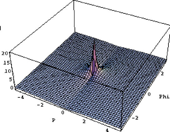
Figure 1: $t=0.001,N=10$

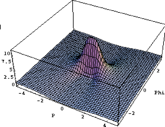
Figure 2: $t=0.1,N=10$

Figure 3: $t=0.001,N=500$

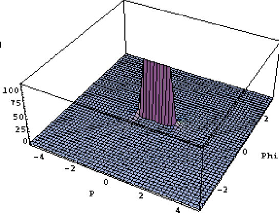
Figure 4: $t=0.001,N=1000$

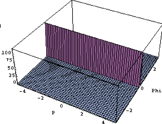
Figure 5: $t=0.001,N=10$

Figures 1 and 2 reveal the bad convergence behaviour of the non-transformed series resulting in grossly misleading plots : taking the same number $N$ of summation terms in the non-transformed series, the one with the higher value of $t$ (figure 2) is the better approximation to the actual situation (figure 5). To improve on the non-transformed series, one has to considerably increase $N$, as shown in figures 3 and 4.

B.1.2 Peakedness of the Overlap Function

We compute the function $|<\psi^{t}_{g},\psi^{t}_{g^{\prime}}>|/(||\psi^{t}_{g}||\;||\psi^{t}_{g^{\prime}}||$ with the parameterizations $g=e^{p_{1}}e^{i\phi},\,g^{\prime}=e^{p_{2}}e^{i\phi^{\prime}}$. W.l.g. we set $\phi^{\prime}=0$, choose the range of $p_{1}$ to be $[p_{2}-5,p_{2}+5]$ and take $\phi\in[-\pi,\pi]$. We compute plots for the values $p_{2}=0,1,2,3,4$ in figures 6 through 10.

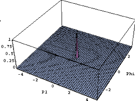
Figure 6: $t=0.001,N=10,p_{2}=0$

Figure 7: $t=0.001,N=10,p_{2}=1$

Figure 8: $t=0.001,N=10,p_{2}=2$

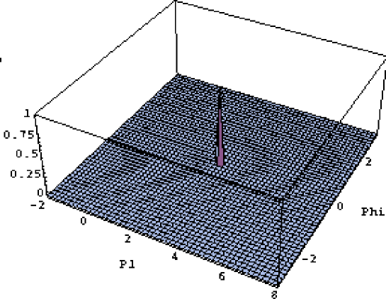
Figure 9: $t=0.001,N=10,p_{2}=3$

Figure 10: $t=0.001,N=10,p_{2}=4$

Finally, figure 11 resolves the exact nature of the peak, exhibiting its Gauss-like structure. Its decay width is compatible with the expected value $\sqrt{t}\approx 0.03$.

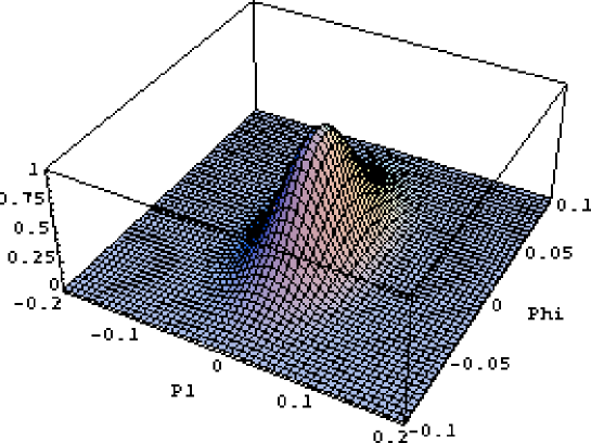
Figure 11: $t=0.001,N=10,p_{2}=0$

B.2 The $SU(2)$ case

B.2.1 Peakedness in the Connection Representation

We numerically compute the function $\frac{|\psi^{t}_{g}(h)|}{\|\psi^{t}_{g}\|}$, with the parametrization $g=e^{-ip^{j}\tau_{j}/2}e^{\theta^{j}\tau_{j}}$. Without restriction, one can chosse $h=1$. For the parameterization vectors we take $p^{j}=(0,0,p)$ and $\theta^{j}=\theta(\sin(\chi),\cos(\phi),\sin(\chi)\sin(\phi),\cos(\chi))$. The variables for each graphic are $\theta\in[0,\pi]$ and $\phi\in[-\pi,\pi]$. Graphics were calculated for all combinations of the values $p=\pm 1,\pm 2$ and $\chi=0,\pi/4,\pi/2,3\pi/4,\pi$. However, since they look completely identical in our resolution we display only the plots with $p=\pm 2$ in figures 12 through 21.

Figure 12: $t=0.001,N=10,p=2,\chi=0$

Figure 13: $t=0.001,N=10,p=2,\chi=\pi/4$

Figure 14: $t=0.001,N=10,p=2,\chi=\pi/2$

Figure 15: $t=0.001,N=10,p=2,\chi=3\pi/4$

Figure 16: $t=0.001,N=10,p=2,\chi=\pi$

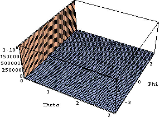
Figure 17: $t=0.001,N=10,p=-2,\chi=0$

Figure 18: $t=0.001,N=10,p=-2,\chi=\pi/4$

Figure 19: $t=0.001,N=10,p=-2,\chi=\pi/2$

Figure 20: $t=0.001,N=10,p=-2,\chi=3\pi/4$

Figure 21: $t=0.001,N=10,p=-2,\chi=\pi$

B.2.2 Peakedness of the Overlap Function

We numerically compute the function $\frac{|\langle\psi^{t}_{g},\psi^{t}_{g^{\prime}}\rangle|}{\|\psi^{t}_{g}\|\;\|\psi^{t}_{g^{\prime}}\|}$, with the parametrizations $g=e^{-ip^{j}\tau_{j}/2}e^{\theta^{j}\tau_{j}}$ $g=e^{-i(p^{\prime})^{j}\tau_{j}/2}e^{(\theta^{\prime})^{j}\tau_{j}}$. Without restriction, one can choose $\theta^{\prime}=0$. For the parameterization vector we take $\theta^{j}=\theta_{0}(\sin(\chi)\cos(\phi),\sin(\chi)\sin(\phi),\cos(\chi))$. The variables for each graphic are $\theta_{0}\in[0,\pi]$ and $p\in[p^{\prime}-5,p^{\prime}+5]$. Graphics were calculated for all combinations of the values $p^{\prime}=\pm 3$, $\chi=0,\pi/2,\pi$ and $\phi=0,\pm\pi/2,\pm\pi$. However, since again all of them look completely identical we display only the plots with $\phi=0$ in figures 22 through 27 for parallel vectors and in figure 28 for orthogonal ones.

Case A: Parallel vectors We choose $p^{j}=(0,0,p)$ and $(p^{\prime})^{j}=(0,0,p^{\prime})$, that is, the momentum vectors are parallel and peakedness is therefore to be expected for $p=p^{\prime}$, independent of the values for $\chi$ and $\phi$.

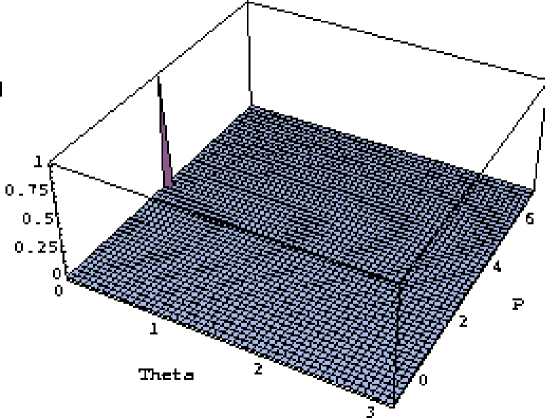
Figure 22: $t=0.001,N=10,p^{\prime}=3,\phi=0,\chi=0$

Figure 23: $t=0.001,N=10,p^{\prime}=3,\phi=0,\chi=\pi/2$

Figure 24: $t=0.001,N=10,p^{\prime}=3,\phi=0,\chi=\pi$

Figure 25: $t=0.001,N=10,p^{\prime}=-3,\phi=0,\chi=0$

Figure 26: $t=0.001,N=10,p^{\prime}=-3,\phi=0,\chi=\pi/2$

Figure 27: $t=0.001,N=10,p^{\prime}=-3,\phi=0,\chi=\pi$

Case B: Orthogonal vectors We now choose $p^{j}=(0,0,p)$ and $(p^{\prime})^{j}=(0,p^{\prime},0)$, that is, the vectors are orthogonal, and therefore the overlap function should approximately vanish for all values of $\chi$ and $\phi$. We have calculated all 30 figures as for case A but will display only one here (figure 28), as they look all the same and expectedly rather boring.

Figure 28: $t=0.001,N=10,p^{\prime}=1,\phi=\pi/2,\chi=\pi$

Finally, figure 29 resolves the exact nature of the peak, exhibiting its Gauss-like structure. Notice that the decay width of the peak is indeed of the order of the expected value $\sqrt{t}\approx 0.03$. This gives an idea of how drastically semi-classical these states will be in applications to quantum gravity in $D=3$ where $t=10^{-64}$ for $a=1$cm !

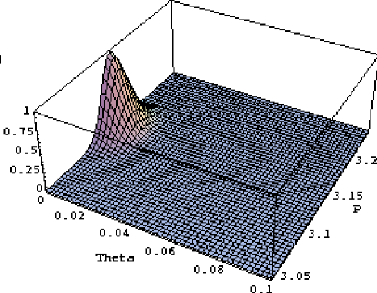
Figure 29: $t=0.001,N=10,p^{\prime}=3.14,\phi=0,\chi=0$

References

- [1]
- [2] A. Ashtekar, Phys. Rev. Lett. 57 (1986) 2244, Phys. Rev. D36 (1987) 1587
- [3] A. Ashtekar, in “Mathematics and General Relativity”, American Mathematical Society, Providence, Rhode Island, 1987
-
[4]
F. Barbero, Phys. Rev. D51 (1995) 5507
F. Barbero, Phys. Rev. D51 (1995) 5498 - [5] T. Thiemann, Physics Letters B 380 (1996) 257-264, gr-qc/960688
-
[6]
R. Gambini, A. Trias, Phys. Rev. D22 (1980) 1380
C. Di Bartolo, F. Nori, R. Gambini, A. Trias, Lett. Nuov. Cim. 38 (1983) 497
R. Gambini, A. Trias, Nucl. Phys. B278 (1986) 436 - [7] C. Rovelli, L. Smolin, Nucl. Phys. B331 (1990) 80
- [8] A. Ashtekar and C.J. Isham, Class. Quantum Grav. 9 (1992) 1433
-
[9]
A. Ashtekar, J. Lewandowski, “Representation
theory of analytic holonomy algebras”, in “Knots and
Quantum Gravity”, J. Baez (ed), Oxford University Press, Oxford, 1994
A. Ashtekar, J. Lewandowski, Journ. Geo. Physics 17 (1995) 191
A. Ashtekar and J. Lewandowski, J. Math. Phys. 36, (1995) 2170 - [10] D. Marolf and J. M. Mourão, “On the support of the Ashtekar-Lewandowski measure”, Commun. Math. Phys. 170 (1995) 583-606
- [11] A. Ashtekar, J. Lewandowski, D. Marolf, J.Mourão, T. Thiemann, Journ. Math. Phys. 36 (1995) 6456-6493, gr-qc/9504018
- [12] R. De Pietri, C. Rovelli, Phys. Rev. D54 (1996) 2664
- [13] R. Gambini, J. Pullin, “Loops, Knots, Gauge Theories and Quantum Gravity”, Cambridge University Press, Cambridge, 1996
- [14] T. Thiemann, Journ. Math. Phys. 39 (1998) 1236-48, hep-th/9601105
- [15] R. De Pietri, Class. Quantum Grav. 14 (1997) 53
- [16] T. Thiemann, Journ. Math. Phys. 39 (1998) 3372-92, gr-qc/9606092
- [17] C. Rovelli, L. Smolin, Nucl. Phys. B 442 (1995) 593; Erratum : Nucl. Phys. B 456 (1995) 734
- [18] A. Ashtekar, J. Lewandowski, Class. Quantum Grav. 14 A55-81 (1997)
-
[19]
R. Loll, Nucl. Phys. B460 (1996) 143
R. Loll, Class. Quantum Grav. 14 (1997) 1725
R. Loll, Nucl. Phys. B500 (1997) 405 - [20] A. Ashtekar, J. Lewandowski, Adv. Theo. Math. Phys. 1 (1997) 388-429
- [21] T. Thiemann, Journ. Math. Phys. 39 (1998) 3347-71, gr-qc/9606091
- [22] T. Thiemann, Class. Quantum Grav. 15 (1998) 839-73, gr-qc/9606089
- [23] T. Thiemann, Class. Quantum Grav. 15 (1998) 875-905, gr-qc/9606090
- [24] T. Thiemann, Class. Quantum Grav. 15 (1998) 1249-80, gr-qc/9705018
- [25] T. Thiemann, Class. Quantum Grav. 15 (1998) 1281-1314, gr-qc/9705019
- [26] T. Thiemann, Class. Quantum Grav. 15 (1998) 1487-1512, gr-qc/9705021
- [27] T. Thiemann, Class. Quantum Grav. 15 (1998) 1463-85, gr-qc/9705020
- [28] T. Thiemann, Class. Quantum Gravity 15 (1998) 1207-47, gr-qc/9705017
- [29] M. Reisenberger, C. Rovelli, Phys. Rev. D56 (1997) 3490-3508
- [30] J. Baez, Class. Quantum Grav. 15 (1998) 1827-58
- [31] F. Markopoulou, L. Smolin, Phys. Rev. D58 (1998) 084032
- [32] J. W. Barret, L. Crane, Class. Quantum Grav. 14 (1997) 2113
- [33] L. Freidel, K. Krasnov, Adv. Theor. Math. Phys. 2 (1999) 1183
- [34] K. Krasnov, Gen. Rel. Grav. 30 (1998) 53-68
- [35] A. Ashtekar, C. Beetle,S. Fairhurst, Class. Quantum Grav. 17 (2000) 1317
- [36] A. Ashtekar, A. Corichi, K. Krasnov, “Isolated horizons : The classical phase space”, gr-qc/9905089
- [37] A. Ashtekar, C. Beetle, S. Fairhurst, Class. Quantum Grav. 16 (1999) L1-L7
- [38] A. Ashtekar, K. Krasnov, “Quantum Geometry and Black Holes”, gr-qc/9804039
- [39] A. Ashtekar, J. Baez, A. Corichi, K. Krasnov, Phys. Rev. Lett. 80 (1998) 904-907
- [40] A. Ashtekar, “Interface of General Relativity, Quantum Physics amd Statistical Mechanics : Some Recent Developments”, gr-qc/9910101
- [41] J. R. Klauder, B.-S. Skagerstam, “Coherent Sates”, World Scientific, Singapore, 1985
- [42] A. Perelomov, “Generalized Coherent States and their Applications”, Springer Verlag, Berlin, 1986
- [43] K. Hepp, Comm. Math. Phys. 35 (1974) 265
-
[44]
L. Smolin, “The classical Limit and the Form of the
Hamiltonian Constraint in non-perturbative Quantum General Relativity”,
gr-qc/9609034
D. Marolf, J. Lewandowski, “Loop Constraints : A Habitat and their Algebra”, gr-qc/9710016
R. Gambini, J. Lewandowski, D. Marolf, J. Pullin, “On the Consistency of the Constraint Algebra in Spin Network Gravity”, gr-qc/9710018 - [45] T. Thiemann, “Quantum Spin Dynamics (QSD) : VIII. The Classical Limit”, to appear
- [46] T. Thiemann, “Gauge Field Theory Coherent States (GCS) : I. General Properties”, hepth/0005233
- [47] T. Thiemann, O. Winkler, “Gauge Field Theory Coherent States (GCS) : III. Ehrenfest Theorems”, hepth/0005234
- [48] T. Thiemann, O. Winkler, “Gauge Field Theory Coherent States (GCS) : IV. Infinite Tensor Product Extension and Thermodynamic Limit”, hep-th/0005235
- [49] T. Thiemann, “Gauge Field Theory Coherent States (GCS) : V. Extension to Higgs Fields and Fermions”, to appear
- [50] H. Sahlmann, T. Thiemann, O. Winkler, “Gauge Field Theory Coherent States (GCS) : VI. Photons and Gravitons Propagating on Quantum Spacetimes”, to appear
- [51] H. Sahlmann, T. Thiemann, O. Winkler, “Gauge Field Theory Coherent States (GCS) : VII. The Non-Perturbative -Ray Burst Effect”, to appear
-
[52]
T. Thiemann, Acta Cosmologica 21 (1995) 145-167, gr-qc/9511049
T. Thiemann, Class. Quantum Gravity 13 (1996) 1383-1403, gr-qc/9511057
T. Thiemann, in : “Symplectic Singularities and Geometry of Gauge Fields”, Banach Center Publications, 39 389-403 (1996), hep-th/9511122 - [53] B. C. Hall, Journ. Funct. Analysis 122 (1994) 103
- [54] B. Hall, Comm. Math. Phys. 184 (1997) 233-250
- [55] A. Ashtekar, J. Lewandowski, D. Marolf, J. Mourão, T. Thiemann, Journ. Funct. Analysis 135 (1996) 519-551, gr-qc/9412014
- [56] T. Thiemann, “Quantum Spin Dynamics (QSD) : VII. Symplectic Structures and Continuum Lattice Formulations of Gauge Field Theories”, hep-th/0005232
- [57] H. Sahlmann, T. Thiemann, O. Winkler, “Gauge Field Theory Coherent States (GCS) : XI. Coherent States for Groups of Higher Rank”, in preparation
- [58] E. Hebey, “Sobolev Spaces on Riemannian Manifolds”, Lecture Notes in Mathematics 1635, Springer Verlag, Berlin, 1996
- [59] S. Lang, “Differential Manifolds”, Addison Wesley, Reading, Massachusetts, 1972
-
[60]
J. Baez, S. Sawin, “Functional Integration on Spaces of
Connections”, q-alg/9507023
J. Baez, S. Sawin, “Diffeomorphism Invariant Spin-Network States”, q-alg/9708005 - [61] J. Lewandowski, T. Thiemann, Class. Quantum Grav. 16 (1999) 2299-2322, gr-qc/9901015
- [62] C. Rovelli, L. Smolin, “Spin networks and quantum gravity” pre-print CGPG-95/4-1, Phys. Rev. D52 (1995) 5743
- [63] J. Baez, Adv. Math. 117 (1996) 253-272
-
[64]
A. Rendall,
Class. Quantum Grav. 10 (1993) 605
A. Rendall, “Adjointness Relations as a Criterion for Choosing an Inner Product”, gr-qc/9403001 - [65] N.M.J. Woodhouse, “Geometric Quantization”, 2nd. edition, Clarendon Press, Oxford, 1991
- [66] S. Bochner, “Vorlesungen über Fouriersche Integrale”, Chelsea Publishing Company, New York, 1948
- [67] H. Urakawa, Osaka Journ. Math. 12 (1975) 285 - 297
- [68] T. Bröcker, T. tom Dieck, “Representations of Compact Lie Groups”, Springer Verlag, New York, 1985
- [69] R. Sexl, H. Urbantke, “Relativität, Gruppen, Teilchen”, Springer Verlag, Berlin, 1984
- [70] R. Gangolli, Acta Math. 121 (1968) 151
- [71] A. R. Edmonds, “Angular Momentum in Quantum Mechanics”, 3rd ed., Princeton University Press, Princeton, 1974
- [72] M.W. Reinsch, J.J. Morehead, “Asymptotics of Clebsch-Gordan Coefficients”, math-ph/9906007
- [73] G. Ponzano, T. Regge, “Semiclassical Limit of Racah Coefficients”, in : “Spectroscopic and Group Theoretical Methods in Physics”, Racah Memorial Volume, ed. F. Bloch, North Holland, Amsterdam, 1968