Monopole in the Dilatonic Gauge Field Theory

D.Karczewska, R.Manka
Department of Astrophysics and Cosmology, Institute of Physics, University of Silesia, Uniwersytecka 4, 40-007 Katowice, Poland.

Abstract

A numerical study of coupled to the dilaton field, static, spherically symmetric monopole solutions inspired by the Kaluza-Klein theory with large extra dimensions are presented. The generalized Prasad-Sommerfield solution is obtained. We show that monopole may have also the dilaton cloud configurations.

1 Introduction

Recently there has been considerable interest in the field theories with large extra spacetime dimensions. In comparison to the standard Kaluza-Klein theory these extra dimensions may be restricted only to the gravity sector of theory while the Standard Model (SM) fields are assumed to be localized on the 4-dimensional spacetime (Antoniadis, Arkani-Hamed, Dimopoulos and Dvali (1998); Antoniadis, Arkani-Hamed, Dimopoulos and Dvali (1998); (Arkani-Hamed Dimopoulos and Dvali (1999)). It is promising scenario from the phenomenological point of view because it shifts the energy scale of unification from $10^{19}\,$GeV o $10-100\,$TeV.

The gauge field theory is extended by inclusion of the dilatonic field in such of theories. Such fields appear also in a natural way in Kaluza-Klein theories (Appelquist, Chodos and Freund, (1987)), superstring inspired theories (Witten (1985); Ferrata, Lüst and Teisen (1989)) and in theories based on the noncommutative geometry approach (Chamseddine and Fröhlich (1993) ).

As previous studies have already shown the inclusion of a dilaton in a pure Yang - Mills theory has consequences already at the classical level. In particular the dilaton Yang - Mills theories possess ’particle - like’ solutions with finite energy which are absent in the pure Yang - Mills case. Analogous equations have recently been obtained for the ’t Hooft - Polyakov monopole model coupled to the dilatonic field (Lavreashvili and Maison (1992)).

2 The dilatonic gauge field theory

Dilatons appear in the higher dimensional theory after the process of the spacetime compactification. The main idea of the theory with large extra dimensions is that the gravity is realized in the more dimensional spacetime (the bulk) while the matter is confined in the four-dimemsional spacetime (the brane). To be clear and simple, we will consider the six-dimensional gravity. Let us now consider the action integral of Einstein-Yang-Mills-Higgs theory in the six-dimensional spacetime:

$${\mathcal{S}}=\int d^{6}x\sqrt{-g_{6}}L,$$ (1)

where $g_{6}=det(g_{MN})$ and $M=\{\mu,\,i\}$, $N=\{\nu,\,j\}$ with $x^{M}=\{x^{\mu},y^{i}\},\,i=1,2$. The metrical tensor in the six-dimensional spacetime can be written:

$$g_{MN}=\left(\begin{array}[]{cc}e^{-2\xi(x)/f_{0}}\overline{g}_{\mu\nu}&0\\ 0&-r_{2}^{2}\delta_{ij}e^{+2\xi(x)/f_{0}}\end{array}\right),$$ (2)

According to above definition we can write:

$$\sqrt{-g_{6}}=\sqrt{-\overline{g}}r_{2}^{2}e^{-2\xi(x)/f_{0}}.$$ (3)

In the equation (2)

$$g_{\mu\nu}=e^{-2\xi(x)/f_{0}}\overline{g}_{\mu\nu}$$ (4)

represents the four-dimensional metric in the Jordan frame while $\overline{g}_{\mu\nu}$ in the Einstein frame. We consider here the Lagrangian of the Einstein-Yang-Mills-Higgs field as follows:

$$L=L_{g}+L_{YMH}\delta(y),$$ (5)

$$L_{g}=-\frac{1}{2\kappa_{6}}(R-2\Lambda),$$ (6)

$$L_{YMH}=-\frac{1}{4}F_{\mu\nu}^{a}F^{a\mu\nu}+\frac{1}{2}D_{\mu}\Phi^{a}D^{\mu}\Phi^{a}-U(\Phi),$$ (7)

where $\kappa_{6}$ is the six-dimensional gravitational coupling. $L$, $L_{g}$, $L_{YMH}$ - describe the total Lagrange function, the gravity in six-dimensional spacetime and the Yang-Mills-Higgs field parts on the brane emdeded in six-dimensional space, respectively. In general non-vanishing cosmological constant ($\Lambda\neq 0$) is possible. This case leads to the interesting monopole solution (Lugo and Shaposhnik (1999, 2000)). In our paper we shall focus our attention on the $\Lambda=0$ case. All calculations should include metric $g_{MN}$ (3), so for example $D^{\mu}=g^{\mu\nu}D_{\nu}$. Let us compactify the six-dimensional spacetime to the four-dimensional Minkowski one on the torus $({\mathcal{M}}_{6}\rightarrow{\mathcal{M}}_{4}\times{\mathcal{S}}^{1}\times{\mathcal{S}}^{1})$. In this paper we assume that the extra dimensions are compactified to two-dimensional torus with a single radius $r_{2}$. The six-dimensional action may be rewritten as:

$${\mathcal{S}}=\int d^{4}x\int d^{2}y\sqrt{-g_{6}}L=\int d^{4}x\sqrt{-\overline{g}}{\mathcal{L}},$$ (8)

where $\int d^{2}y=(2\pi r_{2})^{2}$ and ${\mathcal{L}}$ is the effective Lagrange function in four-dimensional spacetime. The six-dimensional gravitational coupling $\kappa_{6}=8\pi G_{6}$ is convenient to define as

$$G_{6}^{-1}=\frac{1}{(2\pi)^{2}}M^{4},$$

where $M$ - is the energy scale of the compactification ($\sim 10-100\,TeV$). Compactification of the six-dimensional gravity on the torus gives the Lagrangian (8) for the four-dimensional gravity

$$L=-\frac{1}{2\kappa}R_{(4)}$$ (9)

in the Einstein frame, where

$$\frac{1}{\kappa}=\frac{(2\pi r_{2})^{2}}{\kappa_{6}}$$ (10)

is the four-dimensional coupling constant or $\kappa=8\pi G_{N}=8\pi M^{-2}_{Pl}$ . From the above equation (10) we get

$$M^{2}_{Pl}=4\pi M^{4}r_{2}^{2}.$$ (11)

Cosmological consideration (Hall and Smith (1999)) gives the bound $M\sim 100\,TeV$ which corresponds $r_{2}\sim 5.1\times 10^{-5}$ mm from equation (11). Compactification of gravity on the five-dimensional spacetime is rather unpysical ($r_{2}\sim 10\,km$), however the nice five-dimensional spacetime compactivitation was propsed recently (Randal and Sundram (1999a,b)). The Planck mass $M_{Pl}$ (11) is not longer a fundamental constant, it may change during the Universe evolution (Flanagen Tye and Wasserman (1999)). For four-dimensional Minkowski spacetime ($\overline{g}_{\mu\nu}=\eta_{\mu\nu}$)

$$R_{(4)}=\frac{4}{f_{0}^{2}}e^{2\xi(x)/f_{0}}\{-\partial_{\mu}\xi\partial^{\mu}\xi+f_{0}\partial_{\mu}\partial^{\mu}\xi\}.$$ (12)

The last term in the equation (12) can by transform into the first one by differentiating by parts. The parameter $f_{0}$ (or re-scaling of the $\xi(x)$ field) is determined by the Planck mass (at present time) as:

$$f_{0}=\frac{1}{\sqrt{2\pi}}M_{Pl}\sim 4.87\,10^{18}\,GeV/c^{2}$$ (13)

to produce the $1/2$ term in for the dilaton field in (16). The $f_{0}$ parameter determines the dilaton scale $f_{0}$. At the present time $f_{0}$ is rather high, so the interaction with dilatons can be neglected. However, in the early universe when the Planck mass $M_{Pl}$ was smaller (for details see (Flanagen Tye and Wasserman (1999))) also the value of the $f_{0}$ was smaller, too.

As a result of compactification of the six-dimensional Lagrangian we get the Lagrange function for the Yang-Mills-Higgs fields. Fluctuations around the four-dimensional Minkowski

$$\overline{g}_{\mu\nu}=\eta_{\mu\nu}+h_{\mu\nu}(x,y)$$ (14)

will produce interaction with Kaluza-Klein dilatons

$$h_{\mu\nu}(x,y)=\sum_{{\bf n}}h_{\mu\nu}^{{\bf n}}(x)e^{i\frac{2\pi n^{i}y^{i}}{r_{2}}}$$ (15)

with the typical mass scale $M$ (for $n^{i}\neq 0$).

In this paper we shall apply this approach to the simplest $SO(3)$ gauge field theory. The $SO(3)$ gauge field theory has nice monopole solutions (’t Hooft (1976)) which have produced trouble in the cosmology and have been the reason to introduce the idea of inflation. The main idea of this paper is to examine how the monopole solution looks like in the dilatonic gauge field theory inspired by the Kaluza-Klein gravity with the TeV scale.

The dilatonic gauge field theory may described by the Lagrangian (defined by equation (8), in the first approximation when $\overline{g}_{\mu\nu}=\eta_{\mu\nu}$ in the Minkowski spacetime) we get

$${\mathcal{L}}=\frac{1}{2}\partial_{\mu}\xi(x)\partial^{\mu}\xi(x)-\frac{1}{4}e^{2\xi(x)/f_{0}}F_{\mu\nu}^{a}F^{a\mu\nu}+$$ (16)

$$\frac{1}{2}(D_{\mu}\Phi^{a})D^{\mu}\Phi^{a}-e^{-2\xi(x)/f_{0}}U(\Phi),$$

where for $SO(3)$ theory we have:

$$U(\Phi)=\frac{\lambda}{4}(\Phi^{a}\Phi^{a}-v^{2})^{2}$$ (17)

with the $SO(3)$ field strength tensor $F_{\mu\nu}^{a}=\partial_{\mu}W_{\nu}^{a}-\partial_{\nu}W_{\mu}^{a}+g\epsilon_{abc}W_{\mu}^{b}W^{c}_{\mu}$. The $SO(3)$ gauge symmetry rotates the Higgs field $\Phi^{a}$. The covariant derivative is given by $D_{\mu}\Phi^{a}=\partial_{\mu}\Phi^{a}-g\epsilon_{abc}W_{\mu}^{b}\Phi^{c}$. Now we have $D^{\mu}=\eta^{\mu\nu}D_{\nu}$. The Higgs potential has degenerate true vacua forming the sphere $S^{2}$ $(\Phi^{a}\Phi^{a}=v^{2})$. The Euler-Lagrange equations for the Lagrangian (9) are scale - invariant:

$$x^{\mu}\rightarrow x^{\prime}{}^{\mu}=e^{\frac{u}{f_{0}}}x^{\mu},$$ (18)

$$\xi\rightarrow\xi^{\prime}=\xi+u,$$ (19)

$$\Phi\rightarrow\Phi^{\prime}=\Phi,$$ (20)

$$W_{\mu}^{a}\rightarrow W_{\mu}^{a}=e^{-\frac{u}{f_{0}}}W_{\mu}^{a}.$$ (21)

These transformations change the Lagrange function in the following way:

$${\mathcal{L}}\rightarrow{\mathcal{L}}^{\prime}=e^{-\frac{2u}{f_{0}}}{\mathcal{L}.}$$ (22)

This symmetry can be formulated equivalently as a scaling symmetry on the coordinates, and the dilaton is often denoted as a Goldstone boson for dilatations. The origin of the symmetry of the equations of motion is easy understood from the Kaluza-Klein origin of the action. The scale transformations are equivalent to a rescaling of the internal dimensions.

3 The dilatonic monopole.

The monopole scalar field configuration:

$$\Phi^{a} = vh(r)n^{a}=vH(r)\frac{n^{a}}{gr},$$ (23)

where

$$n^{a} = \frac{x^{a}}{r}$$ (24)

describes the ’hedgehog’ structure $n^{a}$ and scalar spherically symmetric field $H(r)$. The $SO(3)$ gauge field is described by the $K(r)$ field:

$$A_{i}^{a}=-\varepsilon_{aij}\frac{1}{gr}n^{j}(1-K(r)).$$ (25)

The dilaton field is described by the $S(x)$ function:

$$\xi(x)=f_{0}S(x)$$ (26)

(if we introduce the dimensionless variable $x=gvr$). The field Euler-Lagrange equations generated by Lagrange function (16) for $H(x)$ and $K(x)$ and $S(x)$ are:

$$H^{\prime\prime}(x)-\frac{2}{x^{2}}H(x)K(x)^{2}+\frac{\varepsilon}{x^{2}}e^{-2S(r)}(x^{2}-H^{2}(x))H(x)=0,$$ (27)

$$K^{\prime\prime}(x)+2K^{\prime}(x)S^{\prime}(x)-\frac{1}{x^{2}}e^{-2S(x)}H(x)^{2}K(x)-\frac{K(x)}{x^{2}}(K(x)^{2}-1)=0,$$ (28)

$$S^{\prime\prime}(x) + \frac{2}{x}S^{\prime}(x)-\alpha^{-1}\frac{1}{x^{4}}e^{2S(x)}\{(1-K(x)^{2})^{2}+2x^{2}K^{\prime}(x)^{2}\}$$

$$+ \frac{1}{2}\varepsilon\alpha^{-1}e^{-2S(r)}(1-\frac{H^{2}(x)}{x^{2}})^{2}=0.$$

In the dilatonic monopole we have two independent dimensionless constants:

$$\varepsilon=\frac{\lambda}{g^{2}},$$ (30)

$$\alpha=(\frac{f_{0}}{v})^{2}.$$ (31)

The mass (or the lowest energy) of the monopole in the rest frame is:

$$M_{mon}=\frac{4\pi v}{g}\int\rho(x)x^{2}dx,$$ (32)

with the energy density given by:

$$\rho(x) = \frac{1}{2}\alpha S^{\prime}(x)^{2}+\frac{1}{2x^{4}}e^{2S(x)}\{(1-K(x)^{2})^{2}+2x^{2}K^{\prime}(x)^{2}\}$$

$$+ \frac{1}{2x^{4}}\{2H(x)^{2}K(x)^{2}+(xH^{\prime}(x)-H(x))^{2}\}$$

$$+ \frac{1}{4}\varepsilon e^{-2S(x)}(1-\frac{H^{2}(x)}{x^{2}})^{2}.$$

Inside the monopole (according to the equations (27), (28) and (3)) the asymptotical behaviour when $x\rightarrow 0$ is given as:

$$K(x)=1-tx^{2}+O(3),$$ (34)

$$H(x)=ux^{2}+O(3),$$ (35)

$$S(x)=a+bx^{2}+O(3),$$ (36)

where u, t, a are local parameters and $b$ must be determined as:

$$b=\frac{24e^{2a}t^{2}-\epsilon e^{-2a}}{12\alpha}.$$ (37)

Far from the monopole core, if $r\rightarrow\infty\,(x\rightarrow\infty)$, both functions H(x) and K(x) should describe the normal vacuum ($\Phi^{a}\Phi^{a}=v^{2}$) with $H\rightarrow x$ and $K\rightarrow 0$ according to the $H,\,K$ function definition (23,25) remembering that $x=gvr$. In this limit the energy density (3) has a simple limit

$$\rho(x)=\frac{1}{2}\alpha S^{\prime}(x)^{2}+\frac{1}{2x^{4}}e^{2S(x)}.$$

The monopole mass in this limit may be rewritten as:

$$M_{mon}=\frac{4\pi v}{g}\int\rho(x)x^{2}dx=$$

$$\frac{4\pi v}{g}\int(\sqrt{\alpha}xS^{\prime}+\frac{1}{x}e^{S})^{2}dx+\frac{4\pi v}{g}\sqrt{\alpha}(e^{S(0)}-e^{S(\infty)}).$$

The first term vanishes if the dilaton field obeys the Bogomolny equation

$$\sqrt{\alpha}xS^{\prime}+\frac{1}{x}e^{S}=0.$$

This equation has a nice solution in the uniform normal vacuum (Bizon (1993))

$$S_{b}=-ln((\sqrt{\alpha}e^{-S(\infty)}-1/x)/\sqrt{\alpha}).$$ (38)

When $r\rightarrow\infty$ dilaton field should disappear in the true vacuum. This demand gives $S(\infty)=0$. So, When $r\rightarrow\infty$ we have the asymptotic behaviour of the solutions

$$H(x)=x\,(1-we^{-\sqrt{2\varepsilon}x})+O(1/x),$$ (39)

$$K(x)=ze^{-x}+O(1/x),$$ (40)

$$S(x)=-ln(\sqrt{\alpha}e^{-S(\infty)}-\frac{1}{\sqrt{\alpha}x})+O(1/x).$$ (41)

Even when $S(\infty)\neq 0$ it may be removed by the dilaton transformation (19). We may solve the differential equations (27, 28, 3) by the iteration method expanding them with respect to $\varepsilon$:

$$H(x)=\sum^{\infty}_{n=0}\varepsilon^{n}H_{n}(x),$$ (42)

$$K(x)=\sum^{\infty}_{n=0}\varepsilon^{n}K_{n}(x),$$ (43)

$$S(x)=\alpha^{-1}\sum^{\infty}_{n=0}\varepsilon^{n}S_{n}(x).$$ (44)

In the first step $(n=0)$ we obtain the equations:

$$H^{\prime\prime}_{0}(x)-\frac{2}{x^{2}}H_{0}(x)K_{0}(x)^{2}=0,$$ (45)

$$K^{\prime\prime}_{0}(x)+\frac{2}{\alpha}K_{0}^{{}^{\prime}}(x)S_{0}^{{}^{\prime}}(x)-\frac{1}{x^{2}}e^{-2S_{0}(x)/\alpha}H_{0}(x)^{2}K_{0}(x)$$ (46)

$$-\frac{K_{0}(x)}{x^{2}}(K_{0}(x)^{2}-1)=0,$$

$$S\prime\prime_{0}(x)+\frac{2}{x}S^{\prime}_{0}(x)-\frac{e^{2S_{0}(x)/\alpha}}{x^{4}}\{(1-K_{0}(x)^{2})^{2}+2x^{2}K^{\prime}_{0}(x)^{2}\}=0,$$ (47)

leading to the Prasad-Sommerfield solution (without the dilaton field $S(x)$). When $\alpha\rightarrow\infty$ we have the Prasad-Sommerfield solution (Prasad and Sommerfield (1975)) and we can find for $H_{0}(x)$ and $K_{0}(x)$ easily as :

$$H_{0}(x)=x/tanh(x)-1,$$ (48)

$$K_{0}(x)=x/sinh(x).$$ (49)

Finding a nice analytical solution for the dilaton field (Fig.3, dotted line)

$$S_{0}(x)=a+\frac{Q_{D}}{x}+\frac{1}{4sinh(x)^{2}x^{2}}(-1+2x^{2}+2xQ_{D}+cosh(2x)$$ (50)

$$-2xQ_{D}\,cosh(2x)-2x\,sinh(2x))$$

was a crucial point of this paper. The leading term for the dilaton field at infinity will be a Coulomb one

$$S_{0}(x)=\frac{Q_{D}}{x}+O(1/x)$$

$Q_{D}$ is the dilatonic charge which originates from the global scale transformation (18-21). The similarity is striking, but we should remember that an electric charge comes from the $\exp(ie\alpha)\in U(1)$ gauge symmetry. The global scale transformation (18-21) is generated by the exponetrial transformation $\exp(u/f_{0})$. However, the asymptotic bevaviour at $x\rightarrow 0$ (36) admits $Q_{D}=0$.

We present the numerical solutions of the coupled set of differential equations (27, 28, 3) in the next section.

4 Numerical solutions

To solve the monopole equations numerically, we need the starting point (Press, Teukolsky and Vetterlino (1992)). To find the starting conditions we can use the solutions found from the variational procedures or from the Prasad-Sommerfield approximation (48, 49, 50). The trial solutions depending on the variational parameters must be postulated in such a way to fulfill the boundary conditions close to the center (34,35,36) of the monopole and at far outside (39,40,41). We postulate the trial solutions:

$$H_{v}(x)=x\frac{(ux+x^{2}(1-e^{-\sqrt{2\varepsilon}x}))}{(1+x^{2})}\sim ux^{2}+O(3),$$ (51)

$$K_{v}(x)=\frac{(1-tx^{2}+zx^{4})}{(1+x^{4}e^{x})}\sim 1-tx^{2}+O(3)$$ (52)

and

$$S_{v}(x)=\frac{(a+bx^{2}+Q_{D}x^{5})}{(1+x^{6})}\sim a+bx^{2}+O(3),$$ (53)

where $O(3)$ are corrections of the third order. For these functions the monopole mass was calculated and the trial functions with minimal energy was found. For the monopole without dilatons we get  the $M_{mon}$ mass of monopole (if $S(x)=0$):

$$M_{mon}=15.886\times 10^{15}\,GeV.$$

The trial functions give the dilaton configuration close to the monopole case without dilatons. The minimal variational configurations for such a dilatonic monopole for $Q_{D}=0$ and $v=10^{16}\,GeV$ are presented on the Table 1. This shows that the mass of the dilatonic monopole dependences on the parameter $\alpha$ ($f_{0}$) and reaches the local minimum (for $\alpha\sim 1$) lower than for monopole without dilatons.

$\alpha$	u	t	z	$M_{dil}$ (1015GeV)
2.37$\times$105	0.2396	0.6021	2.46903	16.4125
2.37$\times$103	0.2396	0.6021	2.46886	16.4107
2.37	0.2591	0.5769	2.2637	15.0284
1	0.2879	0.5389	1.92221	14.4402
0.9	0.2937	0.5327	1.8099	14.4913
0.8	0.3011	0.52609	1.7035	14.6313

Table 1: The dependence of the monopole mass and the parameters u, t, z on the $\alpha$ parameter.

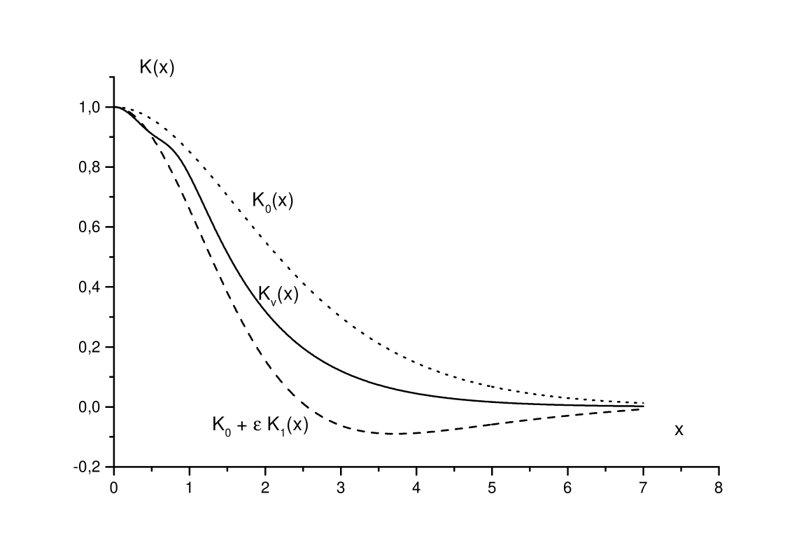
Figure 1: The dependence of the gauge field $K(x)$ on the x parameter. The dotted line corresponds to the Prasad-Sommerfield solution (49), the solid one to the variational solution (52), the dashed line presents the solution of the first iteration.

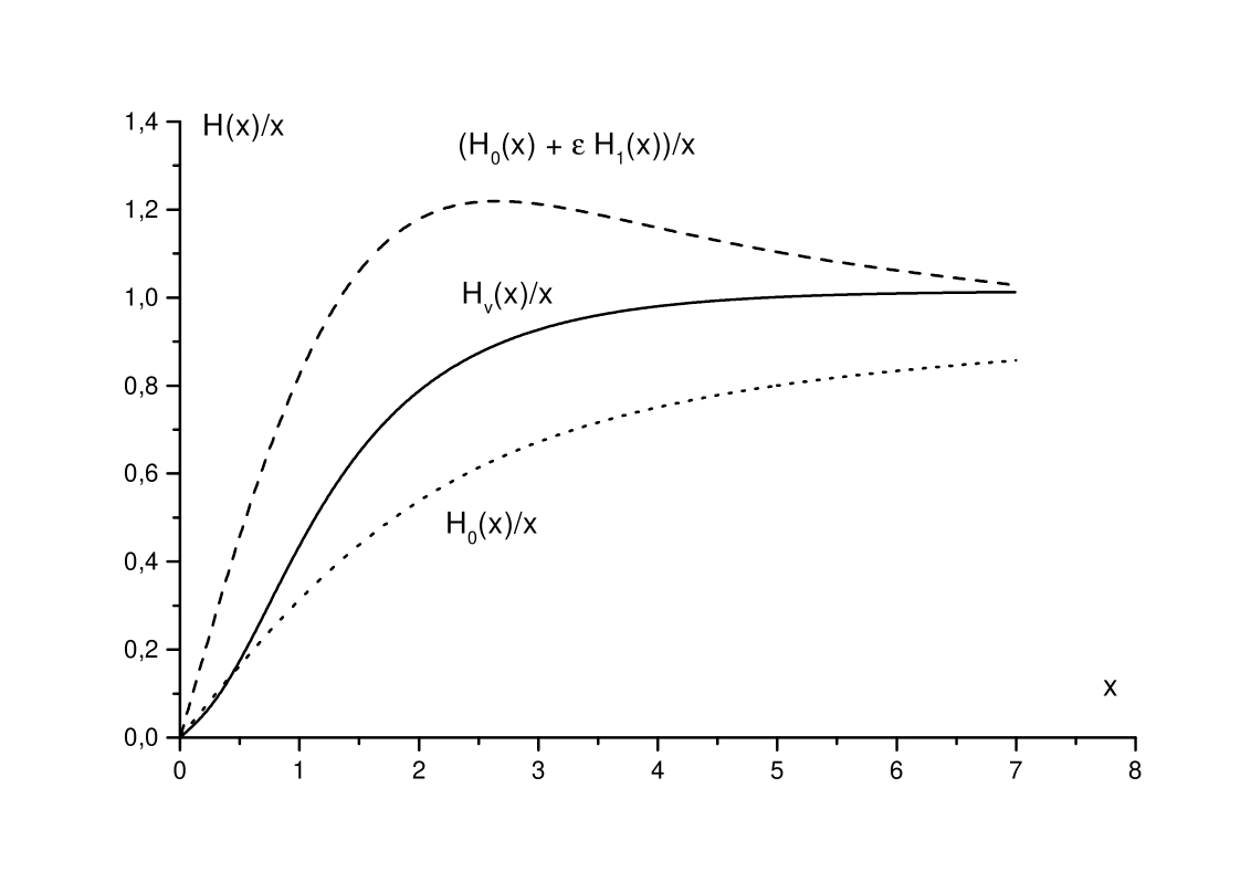
Figure 2: The dependence of the Higgs field $H(x)/x$ on the x parameter. The dotted line corresponds to the Prasad-Sommerfield solution (48), the solid one to the variational solution (51), the dashed line presents the solution of the first iteration.

For the dilatonic monopole the numerical method was independently verified using the Chebyshev polynomial expansion (Michaila (1999)). The monopole solutions for $H(x)$ and $K(x)$ are known very well so our attention is focused on the dilaton solution $S(x)$ especially. The behavior of the $H(x)$ and $K(x)$ solutions determined by the boundary conditions is the same as it is in the presence of the dilaton field.

The Chebyshev method allows to calculate the exact solution of the differential equations for the discrete set of points. The trial function provides the starting data for the numerical solution of the ordinary differential equation (ODE) (the shooting method (Press, Teukolsky and Vetterlino (1992) )) or the Chebyshev functions method. After this preliminary numerical calculation the method based on the Chebyshev polynomial was used.

Clenshaw and Curtis have proposed almost forty years ago an integration method based on the Chebyshev polynomials of the first kind of degree $j$,

$$t_{j}(x)=cos(j*arccos(x)).$$ (54)

Since then, these methods have become standard. Since the Chebyshev polynomials are orthogonal and allows to rewrite the function $f(x)$ as

$$f(x)=\sum_{j=0}\alpha_{j}t_{j}(x),$$ (55)

where (for $j=0$)

$$\alpha_{0}=\frac{1}{n}\sum^{n}_{k=1}f(x_{k})t_{0}(x_{k}),$$ (56)

and (for $j\neq 0$)

$$\alpha_{j}=\frac{2}{n}\sum^{n}_{k=1}f(x_{k})t_{j}(x_{k}).$$ (57)

The grid of $n$ points $x_{k}$ are zeros of the Chebyshev polynomial $t_{j}(x)$. This decomposition allows us to present the derivative of the function $f(x)$ as

$$f^{\prime}(x_{i})=\sum_{k}D_{ik}f(x_{k}),$$ (58)

where the matrix

$$D_{ik}=\sum^{n-1}_{j=0}\frac{1}{c_{j}}t_{j}(x_{k})t_{j}^{\prime}(x_{i}),$$ (59)

and $c_{0}=n$, $c_{j}=n/2$ (at $j\neq 0$). This fact transforms the ordinary differentional equation:

$$\frac{d^{2}f}{dx^{2}}+p(x)\frac{df}{dx}+q(x)=r(x)$$ (60)

into an appropriate linear equation:

$$\sum_{k}A_{ik}f(x_{k})=u_{i}.$$ (61)

So, we can have exact solution for discrete number of points. This method may be also used to nonlinear equation

$$m\frac{d^{2}f}{dx^{2}}+p(x)\frac{df}{dx}+F(f,x)=0.$$ (62)

If we have a starting function $f_{0}$ then we expand $f$ around $f_{0}$

$$f(x)=f_{o}(x)+\varepsilon(x),$$ (63)

and approximate the eq.(62) with the eq.(60) and then solve numerically. The solution may be treat now as a starting function for the next iteration, and so on. The iteration may last so long as an arbitrary precision is reached.

The perturbation around $\varepsilon$ produces the series of differential equations

$$f_{a,b}^{\prime\prime}+\sum_{b}p_{ab,n}(x)f_{b,n}^{\prime}(x)+\sum_{b}q_{ab,n}(x)f_{b,n}(x)=r_{a,n}(x),$$ (64)

where the vector

$$f_{n}=\{H_{n}(x),\,K_{n}(x),\,S_{n}(x)\}.$$ (65)

For example when $n=1$ the first equation ($a=1$) corresponds to $p_{1b}=0$, $q_{11}=2K_{0}^{2}(x)/x^{2}$, $q_{12}=2H_{0}(x)K_{0}(x)/x^{2}$, $r_{1}=exp(-2S_{0}(x)/\alpha)(H_{0}^{2}(x)-x^{2})H_{0}(x)/x^{2}$, and so on.

In the monopole case the starting function are these obtained by the variational method. After expanding around trial functions (51,52,53) we obtain system of the differential equations of the type (60). After that the numerical solution may be obtained on the grid of the $x_{k}$.

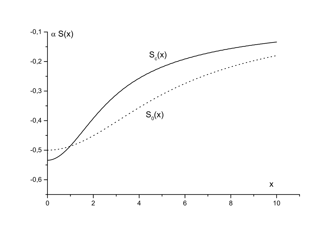
Figure 3: The profile of the dilaton clound $S(x)$. The solid line presents the Chebyshev numerical solution $S_{c}(x)$ and the dotted line is the Prasad-Sommerfield solution $S_{0}(x)$ (50).

The numerical solution for the dilaton field found by the Chebyshev numerical method is presented on the Fig.3 (the solid line).

5 Conclusions

The aim of this paper was to present a numerical study of the classical monopole solutions of the SO(3) theory coupled to the dilaton fields. We have shown that a monopole is surrounded by the dilaton cloud $S(x)$. In the field theories with large extra spacetime dimensions the Planck mass is not longer a fundamental constant and may change itself during the evolution of the universe. As a consequence the parameter $f_{0}$ changes, too. We have shown that the dilatonic monopole reaches the minimal mass when $f_{0}\sim v$ with the mass lower a bit than for monopole without dilatons.

There is analytical solution in the Prasad-Sommerfield limit.

The spherically symmetric dilaton solutions coupled to the gauge field or gravity are interesting in their own and may moreover influence the monopole catalysis.

However in the theory inspired by the Kaluza-Klein theory with large extra dimensions also new interaction with massive ($\sim M$) Kaluza-Klein gravitons takes place. In the four dimensional spacetime the monopole solutions is stable due to the monopole topological charge. Now the interaction with Kaluza-Klein gravitons $h_{\mu\nu}^{{\bf n}}(x)$ may cause disintegration of the monopole.

References

Antoniadis, I., Arkani-Hamed, N., Dimopoulos, S. and Dvali, G., (1998) Phys. Lett. B 436, 257.

Appelquist, T., Chodos, A. Freund, P.G.O.(1987) Modern Kaluza-Klein Theories, Meno Park (Addison-Wesley Publishing Comp.).

Arkani-Hamed, N., Dimopoulos, S. and Dvali, G., (1998). Phys. Lett. B 429, 263,

Arkani-Hamed, N., Dimopoulos, S. and Dvali, G., (1999) Phys. Rev. D 59, 086004, (hep-ph/9807344)

Bizon, P. (1993). Phys. Rev. D, 47, 1656.

Chamseddine, A.H., Fröhlich, J. (1993). Phys. Lett. B 314, 308 (hep-ph/9307209).

Ferrata, S., Lüst, P. and Teisen, S., (1989). Phys.Lett. 233, 147.

Flanagen, E.E., Tye S.-H., Wasserman I., A Cosmology of the Brane World, (hep-ph/9909373).

Hall, L.J., Smith, D.,(1999). Phys. Rev. D 60 085008 (hep-ph/9904267); Banks T., Nelson A., Dine M., (1999). JHEP 9906 014, (hep-th/9903019).

Lavreashvili, G., Maison, D., (1992). Phys. Lett. 295, 67; Lavreashvili, G., Maison, D., Regular and black Hole Solutions of Einstein-Yang-Mills dilaton theory,preprint, MPI-ph/92-115(1992). preprint SLAC-PUB-7479, May 1997.

Lugo A. R., Shaposhnik F.A., (1999). Phys Lett. B 467 43, (hep-th/9909226)

Lugo A. R., Moreno E.F., Shaposhnik F.A., (2000) Phys. Lett. B 473 35 (hep-th/9911209) B.Michaila, Numerical Approximation Using Chebyshev Polynomial Expansion, (physics/9901005); Fox, I., (1962) Computer Journal (UK) 4, 318, ; Clenshaw C.W., Norton H. J., (1963).Computer Journal (UK) 6, 88.

Prasad, M.K., Sommerfield, C.M., (1975). Phys.Rev.Lett. 35, 760.

Press, W.H., Teukolsky, S.A.,Vetterlino, W.T., Numerical Recipies: The art of Scientific Computing, Cambridge University Press (1992).

Randal L., Sundram R., (1999a).Phys. Rev. Lett 83, 3370, (hep-ph/9905221); Randal L., Sundram R., (1999b). Phys. Rev. Lett 83, 4660, (hep-ph/9906064)

’t Hooft, G., (1976). Rev.Lett. 37, (1976), 11; Phys.Rev. D 14, 3432.

Witten, E. (1985). Phys.Lett. B 245, 561.