hep-th/0005236 Anisotropic Four-Dimensional NS-NS String Cosmology

Abstract

An anisotropic (Bianchi type I) cosmology is considered in the four-dimensional NS-NS sector of low-energy effective string theory coupled to a dilaton and an axion-like $H$-field within a de Sitter-Einstein frame background. The time evolution of this Universe is discussed in both the Einstein and string frames.

PACS number(s): 04.20.Jb, 04.65.+e, 98.80.-k

Pre-Big Bang cosmological models [1], based on the low energy limit of the string theory, have been intensively investigated in the recent physics literature [2]-[17]. Generically, in these type of models the dynamics of the Universe is dominated by massless bosonic fields. In the string frame, the four-dimensional NS-NS effective action, which is common to both the heterotic and type II string theories, is given by [18]-[20]

$$\hat{\cal S}=\int d^{4}x\sqrt{-\hat{g}}e^{-2\phi}\left\{\hat{R}+\hat{\kappa}(\nabla\phi)^{2}-\frac{1}{12}\hat{H}_{[3]}^{2}-\hat{U}\right\},$$ (1)

where $H_{\mu\nu\lambda}=\partial_{[\mu}B_{\nu\lambda]}$ is an antisymmetric tensor field, $\hat{\kappa}$ is a generalized dilaton coupling constant and $\hat{U}=\hat{U}(\phi)$ is a dilaton potential. In addition, $\hat{H}_{[3]}^{2}$ means the square of the $H$-field with respect to the metric $\hat{g}_{\mu\nu}$. The low-energy string action posseses a symmetry property, called scale factor duality, which lets us expect that the present phase of the Universe is preceded by an inflationary pre-Big Bang phase. Explicit dual solutions can be constructed for each Bianchi space-time, except the Bianchi class A types VIII and IX models [2].

By means of the conformal rescaling

$$g_{\mu\nu}=e^{-2\phi}\,\hat{g}_{\mu\nu},$$ (2)

the action (1) can be transformed to the so-called Einstein frame as

$${\cal S}=\int d^{4}x\sqrt{-g}\left\{R-\kappa(\nabla\phi)^{2}-\frac{1}{12}e^{-4\phi}\,H_{[3]}^{2}-U\right\},$$ (3)

where $\kappa=6-\hat{\kappa}$, $U=e^{2\phi}\,\hat{U}$ and $H_{[3]}^{2}$ denotes the square of the antisymmetric field by $g_{\mu\nu}$.

Analytic biaxial (two scale factors only) Bianchi type I geometry has been previously considered in [3] for the case with nonvanishing $H_{[3]}$ but without a dilaton field potential, i.e. $U\equiv 0$. Triaxial models with the central deficit charge constrained to zero in the presence of a modulus field (representing the evolution of compact extra dimensions) have been analyzed in [4]. Recently, a study of spatially flat and homogeneous string cosmologies, considering the combined effects of the dilaton, modulus, two-form potential and central charge deficit, and using methods from the qualitative theory of differential equations (phase portrait analysis) has been presented in [5],

The general Bianchi type I space-time for arbitrary dimensional dilaton gravities, with vanishing antisymmetric tensor $H_{\mu\nu\lambda}$ and in the presence of an exponential type dilaton field potential, have been obtained in both the Einstein and string frames [6].

It is the purpose of the present letter to consider, in the framework of a four-dimensional Bianchi type I geometry, the effects on the dynamics and evolution of the early Universe of a non-vanishing antisymmetric field and of a string frame exponential type dilaton field potential.

In the Einstein frame the field equations, which follow from variation of (3), are given by

$$R_{\mu\nu}-\kappa\partial_{\mu}\phi\partial_{\nu}\phi-\frac{1}{2}g_{\mu\nu}U\qquad\qquad$$ (4)

$$-\frac{1}{4}e^{-4\phi}\left(H_{\mu\alpha\beta}H_{\nu}{}^{\alpha\beta}-\frac{1}{3}g_{\mu\nu}H^{2}\right) = 0,$$ (5)

$$\nabla_{\mu}\left(e^{-4\phi}H^{\mu\nu\lambda}\right) = 0,$$ (6)

$$\nabla^{2}\phi+\frac{1}{6\kappa}e^{-4\phi}H^{2}-\frac{1}{2\kappa}\frac{\partial U}{\partial\phi} = 0.$$ (7)

Moreover, the $H$-field must satisfy the integrability condition (Bianchi identity) $\partial_{[\mu}H_{\nu\lambda\rho]}=0$.

In four dimensions, every three-form field can be dualized to a pseudoscalar. Thus, an appropriate ansatz for the $H$-field is [3]

$$H^{\mu\nu\lambda}=\frac{1}{\sqrt{-g}}\,e^{4\phi}\,\epsilon^{\mu\nu\lambda\rho}\,\partial_{\rho}h,$$ (8)

where $\epsilon^{\mu\nu\lambda\rho}=-\delta^{\mu}_{[0}\delta^{\nu}_{1}\delta^{\lambda}_{2}\delta^{\rho}_{3]}$ is the total antisymmetric tensor and $h=h(t)$ is the Kalb-Ramond axion field. Then the field equation (6) is satisfied automatically and the Bianchi identity becomes

$$\partial_{\mu}\left(\sqrt{-g}\,e^{4\phi}\,\partial^{\mu}h\right)=0.$$ (9)

Moreover, we shall assume that in the string frame the dilaton field potential is of exponential type

$$\hat{U}(\phi)=\Lambda\,e^{-2\phi},$$ (10)

with $\Lambda$ a non-negative constant (de Sitter space-time). Therefore in the Einstein frame the effect of the potential is identical to that of a cosmological constant, $U(\phi)=\Lambda$.

For the Bianchi type I space-time, in the Einstein frame,

$$ds^{2}=-dt^{2}+\sum_{i=1}^{3}a_{i}^{2}(t)\left(dx^{i}\right)^{2},$$ (11)

and the ansatz (8,10), the field equations (5,7,9) take the form

$$3\dot{\theta}+\sum_{i=1}^{3}\theta_{i}^{2}+\kappa\dot{\phi}^{2}+\frac{1}{2}e^{4\phi}\,\dot{h}^{2}-\frac{1}{2}\Lambda = 0,$$ (12)

$$\frac{1}{V}\frac{d}{dt}(V\theta_{i})-\frac{1}{2}\Lambda = 0,\,\,i=1,2,3,$$ (13)

$$\ddot{h}+3\theta\dot{h}+4\dot{\phi}\dot{h} = 0,$$ (14)

$$\frac{1}{V}\frac{d}{dt}(V\dot{\phi})-\frac{1}{\kappa}e^{4\phi}\dot{h}^{2} = 0,$$ (15)

where we have introduced the volume scale factor, $V:=\prod_{i=1}^{3}a_{i}$, directional Hubble factors, $\theta_{i}:=\dot{a}_{i}/a_{i},\,i=1,2,3$, and the mean Hubble factor, $\theta:=\sum_{i=1}^{3}\theta_{i}/3=\dot{V}/3V$. We shall also introduce two basic physical observational quantities in cosmology: the mean anisotropy parameter, $A:=\sum_{i=1}^{3}(\theta_{i}-\theta)^{2}/3\theta^{2}$, and the deceleration parameter, $q=\frac{d}{dt}\theta^{-1}-1$.

By summing equations (13) we obtain

$$\frac{1}{V}\frac{d}{dt}(V\theta)=\frac{1}{2}\Lambda,$$ (16)

which, together with (13), leads to

$$\theta_{i}=\theta+K_{i}V^{-1},\quad i=1,2,3,$$ (17)

with $K_{i},\,i=1,2,3$ being constants of integration satisfying $\sum_{i=1}^{3}K_{i}=0$.

It is worth noticing that, in this framework, the geometry of the considered Universe, which is described by $a_{i}(t),\,i=1,2,3$, is determined only by the existence of the cosmological constant $\Lambda$ and is “decoupled” from the matter fields $\phi$ and $H$. (The effect of matter fields is presented in the magnitude of the parameters, i.e. constants of integration.)

From equation (16) we obtain the time evolution of the mean Hubble factor,

$$\theta(\tau)=\sqrt{\frac{\Lambda}{6}}\coth\tau,$$ (18)

leading to

$$V(\tau) = V_{0}\sinh\tau,$$ (19)

$$a_{i}(\tau) = a_{i0}\sinh^{\alpha_{i}^{+}}\frac{\tau}{2}\cosh^{\alpha_{i}^{-}}\frac{\tau}{2},\quad i=1,2,3,$$ (20)

where $\tau:=\sqrt{3\Lambda/2}(t-t_{0})$ and $\alpha_{i}^{\pm}:=1/3\pm\sqrt{2/3\Lambda}K_{i}/V_{0}$. The mean anisotropy and the deceleration parameter are given by

$$A(\tau) = \frac{2K^{2}}{\Lambda V_{0}^{2}}\,\hbox{sech}^{2}\tau,$$ (21)

$$q(\tau) = 3\,\hbox{sech}^{2}\tau-1,$$ (22)

where $K^{2}=\sum_{i=1}^{3}K_{i}^{2}$.

Equation (14) can be integrated to give

$$\dot{h}=C\,e^{-4\phi}\,V^{-1},$$ (23)

with $C$ a constant of integration. Thus the dynamics of the dilaton field in the Einstein frame is described by the following differential equation

$$\sinh\tau\frac{d}{dt}\left(\sinh\tau\,\dot{\phi}\right)=\frac{C^{2}}{\kappa V_{0}^{2}}e^{-4\phi},$$ (24)

with the general solution

$$e^{2\phi(\tau)}=\varphi_{0}^{2}\left(\tanh^{\omega}\frac{\tau}{2}+\tanh^{-\omega}\frac{\tau}{2}\right),$$ (25)

where we denote $\omega:=\sqrt{8\phi_{0}/3\Lambda}/V_{0}$, $\varphi_{0}^{2}:=\sqrt{C^{2}/8\kappa\phi_{0}}$ and $\phi_{0}>0$ is a constant of integration. The antisymmetric tensor field is given by

$$h(\tau)=h_{0}+\frac{\kappa\sqrt{\phi_{0}}}{C}\,\frac{\tanh^{2\omega}\frac{\tau}{2}-1}{\tanh^{2\omega}\frac{\tau}{2}+1},$$ (26)

with $h_{0}$ an arbitrary constant.

The integration constants must satisfy the consistency condition,

$$K^{2}=\Lambda V_{0}^{2}-\kappa\phi_{0},$$ (27)

which follows from equation (12).

In the case of vanishing cosmological constant, $\Lambda\equiv 0$, the general solution in the Einstein frame of the gravitational field equations for a Bianchi type I geometry with dilaton and Kalb-Ramond axion fields is given by:

$$\theta(t) = \frac{1}{3t},\qquad V(t)=V_{0}t,$$ (28)

$$a_{i}(t) = a_{i0}\,t^{1/3+K_{i}/V_{0}},\quad i=1,2,3,$$ (29)

$$A = 3K^{2}V_{0}^{-2}=const.,\qquad q=2=const.,$$ (30)

$$e^{2\phi(t)} = \varphi_{0}^{2}\,\left(t^{\alpha}+t^{-\alpha}\right),$$ (31)

$$h(t) = h_{0}-\frac{2\kappa\sqrt{\phi_{0}}}{C}\left(t^{2\alpha}+1\right)^{-1},$$ (32)

together with the consistency condition

$$K^{2}=\frac{2}{3}V_{0}^{2}-\kappa\phi_{0},$$ (33)

where $\alpha=2\sqrt{\phi_{0}}/V_{0}$.

In order to find the general solution of the gravitational field equations in the string frame with the line element

$$d\hat{s}^{2}=-d\hat{t}^{2}+\sum_{i=1}^{3}\hat{a}_{i}^{2}(\hat{t})\left(dx^{i}\right)^{2},$$ (34)

we must perform the conformal transformation (2). To obtain a simpler mathematical form of the equations we shall introduce a new variable $\eta=\tanh\tau/2$, $\eta\in[0,1]$ and denote $\hat{\varphi}_{0}:=\sqrt{8/3\Lambda}\,\varphi_{0}$. Then the string frame time evolution of the Bianchi type I space-time with dilaton and Kalb-Ramond axion fields and an exponential type dilaton potential can be expressed in the following exact parametric form:

$$\hat{t}(\eta) = \hat{t}_{0}+\hat{\varphi}_{0}\int\frac{\sqrt{\eta^{\omega}+\eta^{-\omega}}}{1-\eta^{2}}\,d\eta,$$ (35)

$$\hat{V}(\eta) = \hat{V}_{0}\,(\eta^{\omega}+\eta^{-\omega})^{3/2}\frac{\eta}{1-\eta^{2}},$$ (36)

$$\hat{\theta}(\eta) = \frac{1}{3\hat{\varphi}_{0}}\frac{1-\eta^{2}}{\eta\sqrt{\eta^{\omega}\!+\!\eta^{-\omega}}}\left(\frac{3\omega}{2}\frac{\eta^{\omega}\!-\!\eta^{-\omega}}{\eta^{\omega}\!+\!\eta^{-\omega}}\!+\!\frac{1\!+\!\eta^{2}}{1\!-\!\eta^{2}}\right),$$ (37)

$$\hat{a}_{i}(\eta) = \hat{a}_{i0}\frac{\eta^{\alpha_{i}^{+}}\sqrt{\eta^{\omega}+\eta^{-\omega}}}{(1-\eta^{2})^{1/3}}\quad i=1,2,3,$$ (38)

$$\hat{A}(\eta) = \frac{2K^{2}}{\Lambda V_{0}^{2}}\left(\frac{3\omega}{2}\,\frac{\eta^{\omega}-\eta^{-\omega}}{\eta^{\omega}+\eta^{-\omega}}+\frac{1+\eta^{2}}{1-\eta^{2}}\right)^{-2},$$ (39)

$$\hat{q}(\eta) := \frac{d}{d\hat{t}}\hat{\theta}^{-1}-1=\frac{1-\eta^{2}}{\hat{\varphi}_{0}\sqrt{\eta^{\omega}+\eta^{-\omega}}}\,\frac{d}{d\eta}\hat{\theta}^{-1}-1.$$ (40)

In the case of a vanishing cosmological constant the string frame solution of the gravitational field equations with dilaton and axion fields is given again in a parametric form by:

$$\hat{t}(t) = \hat{t}_{0}+\varphi_{0}\,\int\sqrt{t^{\alpha}+t^{-\alpha}}\,dt,$$ (41)

$$\hat{V}(t) = \hat{V}_{0}\,t\,(t^{\alpha}+t^{-\alpha})^{3/2},$$ (42)

$$\hat{\theta}(t) = \varphi_{0}^{-1}\,\left(\frac{\alpha}{2}\,\frac{t^{\alpha}-t^{-\alpha}}{t^{\alpha}+t^{-\alpha}}+\frac{1}{3}\right)\frac{1}{t(t^{\alpha}+t^{-\alpha})^{1/2}},$$ (43)

$$\hat{a}_{i}(t) = \hat{a}_{i0}\,t^{1/3+K_{i}/V_{0}}\sqrt{t^{\alpha}+t^{-\alpha}},\quad i=1,2,3,$$ (44)

$$\hat{A}(t) = \frac{K^{2}}{3V_{0}^{2}}\,\left(\frac{\alpha}{2}\frac{t^{\alpha}-t^{-\alpha}}{t^{\alpha}+t^{-\alpha}}+\frac{1}{3}\right)^{-2},$$ (45)

$$\hat{q}(t) = 2-\frac{\alpha\left(\frac{1}{3}\,\frac{t^{\alpha}-t^{-\alpha}}{t^{\alpha}+t^{-\alpha}}+\frac{\alpha}{2}\right)}{\left(\frac{\alpha}{2}\,\frac{t^{\alpha}-t^{-\alpha}}{t^{\alpha}+t^{-\alpha}}+\frac{1}{3}\right)^{2}}.$$ (46)

In the present letter we have presented the exact solution of the gravitational field equations for a Bianchi type I space-time with dilaton and axion fields in both the Einstein and string frames. In the Einstein frame the evolution of the Bianchi type I Universe in the presence of a cosmological constant starts from a singular state, but with finite values of the mean anisotropy and deceleration parameter. In the large time limit the mean anisotropy tends to zero, $A\to 0$, and the Universe will end in an isotropic inflationary de Sitter phase with a negative deceleration parameter, $q<0$. In the large time limit the dilaton and axion fields become constants. Moreover, in the Einstein frame, the dynamics and evolution of the Universe is determined only by the presence of a cosmological constant and there is no coupling between the metric and the dilaton and axion fields.

In the string frame the dilaton and axion fields are coupled to the metric. Depending on the values of the constant $\omega$ there are two distinct types of behavior. In the first type of evolution, corresponding to $\omega<2/3$, the Universe starts from a singular state with zero values of the scale factors, $\hat{a}_{i}(0)=0,\,i=1,2,3$ and expands indefinitely. In the second case, when $\omega>2/3$, the Bianchi type I Universe starts its evolution with infinite values of the scale factors and collapses to a bounce state, corresponding to minimum finite non-zero values of the scale factors. From this non-singular state the Universe starts to expand, ending in an isotropic and inflationary era. The values of the physical quantities at the bounce correspond to the values of $\eta$ satisfying the equation $d\hat{V}/d\eta=0$ or

$$\frac{(\eta^{\omega}+\eta^{-\omega})^{3/2}}{1-\eta^{2}}\left(\frac{3\omega}{2}\frac{\eta^{\omega}-\eta^{-\omega}}{\eta^{\omega}+\eta^{-\omega}}+\frac{1+\eta^{2}}{1-\eta^{2}}\right)=0.$$ (47)

The string frame time variation of the volume scale factor of the Bianchi type I space-time for different values of $\omega$ is presented in Fig.1. Independently of which type of evolution classified by the value of $\omega$, in the presence of an exponential type dilaton potential and of an axion field, the Bianchi type I Universe always isotropizes in the large time limit, $\hat{A}\to 0$ for $\hat{t}\to\infty$. But the dynamics of the mean anisotropy factor is very different for the two types of evolution. During the collapse to the bounce the mean anisotropy increases to an infinite value and then, during the expansionary period, tends rapidly to zero. Hence in this case the expansionary evolution of the Bianchi type I Universe starts with non-singular scale factors and with maximum anisotropy. The string frame time variation of the anisotropy parameter and of the deceleration parameter are represented in the Figures 2 and 3, respectively. In the string frame and in the presence of a dilaton potential the large time evolution is inflationary for all times and for all $\omega$.

In the absence of a cosmological constant or a dilaton field potential the Universe does not isotropize. In this case the Einstein frame mean anisotropy is constant for all times and the evolution is of the Kasner type. In the string frame the mean anisotropy tends, in the large time limit, to a constant non-zero value, hence showing that the Universe will never end in an isotropic flat Robertson-Walker type phase. The deceleration parameter in both frames is positive for all times and an inflationary evolution is also impossible. Therefore string cosmological models involving only pure dilaton and axion fields do not have, at least in the case of Bianchi type I anisotropic geometries, the ability of providing realistic cosmological models. To obtain a transition from an anisotropic state to an isotropic inflationary one the “good old” cosmological constant is still the key ingredient.

FIG. 1.: String frame evolution of the volume scale factor $\hat{V}$ for different values of the parameter $\omega$: $\omega=0.1$ (full curve), $\omega=0.5$ (dotted curve), $\omega=0.75$ (short dashed curve) and $\omega=0.9$ (long dashed curve). We have used the normalization $\hat{V}_{0}=1$ and $\hat{t}_{0}=0$

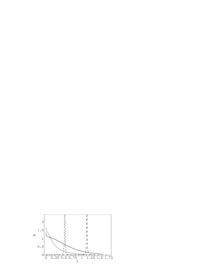
FIG. 2.: String frame time variation of the mean anisotropy parameter $\hat{A}$ for different values of $\omega$: $\omega=0.1$ (full curve), $\omega=0.5$ (dotted curve), $\omega=0.75$ (short dashed curve) and $\omega=0.9$ (long dashed curve). We have used the normalization $2K^{2}/V_{0}^{2}\Lambda=1$.

FIG. 3.: Dynamics of the deceleration parameter $\hat{q}$ in the string frame for different values of $\omega$: $\omega=0.1$ (full curve), $\omega=0.5$ (dotted curve), $\omega=0.75$ (short dashed curve) and $\omega=0.9$ (long dashed curve).

One of the authors (CMC) would like to thank prof. J.M. Nester for useful comments. The work of CMC was supported in part by the National Science Council (Taiwan) under grant NSC 89-2112-M-008-016.

REFERENCES

• [1] M. Gasperini and G. Veneziano, Pre-Big Bang in String Cosmology, Astropart. Phys. 1 (1993) 317-339; hep-th/9211021.
• [2] E. Di Pietro and J. Demaret, Scale Factor Duality in String Bianchi Cosmologies, Int. J. Mod. Phys. D8 (1999) 349-361; gr-qc/9903063.
• [3] E. J. Copeland, A. Lahiri and D. Wands, Low Energy Effective String Cosmology, Phys. Rev. D50 (1994) 4868-4880; hep-th/9406216.
• [4] E. J. Copeland, A. Lahiri and D. Wands, String Cosmology with a Time-Dependent Antisymmetric Tensor Potential, Phys. Rev. D51 (1995) 1569-1576; hep-th/9410136.
• [5] A. P. Billyard, A. A. Coley and J. E. Lidsey, Qualitative Analysis of String Cosmologies, Phys. Rev. D59 (1999) 123505; qr-qc/9903095.
• [6] C.-M. Chen, T. Harko and M. K. Mak, Bianchi Type I Cosmologies in Arbitrary Dimensional Dilaton Gravities, hep-th/0004096.
• [7] R. Easther, K. Maeda and D. Wands, Tree Level String Cosmology, Phys. Rev. D53 (1996) 4247-4256; hep-th/9509074.
• [8] M. Gasperini and R. Ricci, Homogeneous Conformal String Backgrounds, Class. Quant. Grav. 12 (1995) 677-688; hep-th/9501055.
• [9] J. D. Barrow and K. E. Kunze, Spatially Homogeneous String Cosmologies, Phys. Rev. D55 (1997) 623-629; hep-th/9608045.
• [10] J. D. Barrow and K. E. Kunze, Inhomogeneous String Cosmologies, Phys. Rev. D56 (1997) 741-752; hep-th/9701085.
• [11] A. L. Maroto and I. L. Shapiro, On the Inflationary Solutions in Higher Derivative Gravity with Dilaton Field, Phys. Lett. B414 (1997) 34-44; hep-th/9706179.
• [12] A. Lukas, B. A. Ovrut and D. Waldram, The Cosmology of M-Theory and Type II Superstrings, hep-th/9802041.
• [13] R. Brandenberger, R. Easther and J. Maia, Non-singular Dilaton Cosmology, JHEP 9809 (1998) 007; gr-qc/9806111.
• [14] K. E. Kunze and R. Durrer, Anisotropic ‘Hairs’ in String Cosmology, gr-qc/9912081.
• [15] D. Clancy, A. Feinstein, J. E. Lidsey and R. Tavakol, Tilted String Cosmologies, Phys. Lett. B451 (1999) 303-308; gr-qc/9903022.
• [16] G. F. R. Ellis, D. C. Roberts, D. Solomons and P. K. S. Dunsby, Using the Dilaton Potential to Obtain String Cosmology Solutions, gr-qc/9912005.
• [17] R. Durrer and M. Sakellariadou, Kalb-Ramond Axion Production in Anisotropic String Cosmologies, hep-ph/0003112.
• [18] C. G. Callan, E. J. Martinec, M. J. Perry and D. Friedan, Strings in Background Fields, Nucl. Phys. B262 (1985) 593-609.
• [19] C. Lovelace, Stability of String Vacua. 1. A New Picture of the Renormalization Group, Nucl. Phys. B273 (1986) 413-467.
• [20] L. J. Romans, Massive $N=2A$ Supergravity in Ten-Dimensions, Phys. Lett. B169 (1986) 374-380.