Renormalization-Scale-Invariant PQCD Predictions for $R_{e^{+}e^{-}}$ and the Bjorken Sum Rule at Next-to-Leading Order

Abstract

We discuss application of the physical QCD effective charge $\alpha_{V}$, defined via the heavy-quark potential, in perturbative calculations at next-to-leading order. When coupled with the Brodsky-Lepage-Mackenzie prescription for fixing the renormalization scales, the resulting series are automatically and naturally scale and scheme independent, and represent unambiguous predictions of perturbative QCD. We consider in detail such commensurate scale relations for the $e^{+}e^{-}$ annihilation ratio $R_{e^{+}e^{-}}$ and the Bjorken sum rule. In both cases the improved predictions are in excellent agreement with experiment.

I Introduction

One of the most important problems in making reliable predictions in perturbative QCD is dealing with the dependence of the truncated perturbative series on the choice of renormalization scale $\mu$ and scheme $s$ for the QCD coupling $\alpha_{s}(\mu)$. Consider a physical quantity ${\cal O}$, computed in perturbation theory and truncated at next-to-leading order (NLO) in $\alpha_{s}$:

$${\cal O}=\alpha_{s}(\mu)\left[1+\left(A_{1}(\mu)+B_{1}(\mu)n_{f}\right){\alpha_{s}(\mu)\over\pi}+\cdots\right]\;,$$ (1)

where $n_{f}$ is the effective number of quark flavors. The finite-order expression depends on both $\mu$ and the choice of scheme used to define the coupling. In fact, Eqn. (1) can be made to take on essentially any value by varying $\mu$ and the renormalization scheme, which are a priori completely arbitrary. The scale/scheme problem is that of choosing $\mu$ and the scheme $s$ in an “optimal” way, so that an unambiguous theoretical prediction, ideally including some plausible estimate of theoretical uncertainties, can be made.

For any given observable there is no rigorously correct way to make this choice in general. However, a particular prescription may be supported to a greater or lesser degree by general theoretical arguments and, a posteriori, by its success in practical applications. From these perspectives, a particularly successful method for choosing the renormalization scale is that proposed by Brodsky, Lepage and MacKenzie [1]. In the BLM procedure, the renormalization scales are chosen such that all vacuum polarization effects from fermion loops are absorbed into the running couplings. A principal motivation for this choice is that it reduces to the correct prescription in the case of Abelian gauge theory. Furthermore, the BLM scales are physical in the sense that they typically reflect the mean virtuality of the gluon propagators. Another important advantage of the method is that it “pre-sums” the large and strongly divergent terms in the pQCD series which grow as $n!(\alpha_{s}\beta_{0})^{n}$, i.e., the infrared renormalons associated with coupling constant renormalization.

Dependence on the renormalization scheme can be avoided by considering relations between physical observables only. By the general principles of renormalization theory, such a relation must be independent of any theoretical conventions, in particular the choice of scheme in the definition of $\alpha_{s}$. A relation between physical quantities in which the BLM method has been used to fix the renormalization scales is known as a “commensurate scale relation” (CSR) [2]. An important example is the generalized Crewther relation [2, 3], in which the radiative corrections to the Bjorken sum rule for deep inelastic lepton-proton scattering at a given momentum transfer $Q$ are predicted from measurements of the $e^{+}e^{-}$ annihilation cross section at a commensurate energy scale $\sqrt{s}\propto Q$.

A useful tool in these analyses is the concept of an “effective charge.” Any perturbatively calculable observable can be used to define an effective charge by incorporating the entire radiative correction into its definition. Since such a charge is itself a physical observable, perturbation theory in terms of it, with the BLM prescription setting the scales, is automatically renormalization scale- and scheme-independent.

In this paper we shall use the heavy quark potential to define an effective QCD coupling $\alpha_{V}$, and construct scale-commensurate expansions of various other QCD observables in terms of it. A recent calculation of the heavy quark potential at NNLO [4] allows the relevant BLM scales to be determined through NLO. The resulting relations can be tested directly for agreement with available data, and in addition may be used to study various phenomenological forms for the heavy quark potential at moderate to low $Q^{2}$.

We begin by outlining the BLM approach and the idea of commensurate scale relations. We also introduce physical effective charges asociated with the heavy quark potential, the $e^{+}e^{-}$ annihilation cross section and the Bjorken sum rule. In section III we then construct the NLO scale-commensurate expansions of these observables in terms of $\alpha_{V}$, and compare the results to the available data using a simple parameterization for $\alpha_{V}$ which is fit to a lattice calculation. In general the agreement is excellent. In section IV we present some discussion of the results and our conclusions.

II BLM Scale Fixing

At lowest order the BLM approach is straightforward to motivate. The term involving $n_{f}$ in Eqn. (1) arises solely from quark loops in vacuum polarization diagrams. In QED these are the only contributions responsible for the running of the coupling, and thus it is natural to absorb them into the definition of the coupling. The BLM procedure is the analog of this approach in QCD. Specifically, we rewrite Eqn. (1) in the form

$${\cal O}=\alpha_{s}(\mu)\left[1-\left({3\beta_{0}B_{1}(\mu)\over 2}\right){\alpha_{s}(\mu)\over\pi}+\cdots\right]\left[1+\left(A_{1}(\mu)+{33B_{1}(\mu)\over 2}\right){\alpha_{s}(\mu)\over\pi}+\cdots\right]\;,$$ (2)

correct to order $\alpha_{s}^{2}$, where $\beta_{0}=11-{2n_{f}/3}$ is the lowest-order QCD beta function. The first term in square brackets can then be absorbed by a redefinition of the renormalization scale in the leading-order coupling, using

$$\alpha_{s}(\mu^{*})=\alpha_{s}(\mu)\left[1-{\beta_{0}\alpha_{s}(\mu)\over 2\pi}\ln\left(\mu^{*}/\mu\right)+\cdots\right]\;.$$ (3)

That is, the BLM procedure consists of defining the prediction for ${\cal O}$ at this order to be

$${\cal O}=\alpha_{s}(\mu^{*})\left[1+\left(A_{1}(\mu)+{33B_{1}(\mu)\over 2}\right){\alpha_{s}(\mu^{*})\over\pi}+\cdots\right]\;,$$ (4)

where

$$\mu^{*}\equiv\mu e^{3B_{1}(\mu)}\;.$$ (5)

Note that knowledge of the NLO term in the expansion is necessary to fix the scale at LO. Thus the scale occurring in the highest term in the expansion will in general be unknown. A natural prescription is to set this scale to be the same as that in the next-to-highest-order term.

A very important feature of this prescription is that $\mu^{*}$ is actually independent of $\mu$. (This follows from considering the $\mu$ dependence of $B_{1}(\mu)$. For a detailed discussion of this point, see Ref. [1].) Thus pQCD predictions using the BLM procedure are unambiguous.

The same basic idea can be extended to higher orders, by systematically shifting $n_{f}$ dependence into the renormalization scales order by order. Full details of this procedure may be found in Refs. [5, 6]. The result is that a general expansion

$${\alpha_{s}(\mu)\over\pi}+\left(A_{1}+B_{1}n_{f}\right)\left({\alpha_{s}(\mu)\over\pi}\right)^{2}+\left(A_{2}+B_{2}n_{f}+C_{2}n_{f}^{2}\right)\left({\alpha_{s}(\mu)\over\pi}\right)^{3}+\cdots$$ (6)

is replaced by a series of the form

$${\alpha_{s}(\mu^{*})\over\pi}+\widetilde{A}_{1}\left({\alpha_{s}(\mu^{**})\over\pi}\right)^{2}+\widetilde{A}_{2}\left({\alpha_{s}(\mu^{***})\over\pi}\right)^{3}+\cdots\;.$$ (7)

In general a different scale appears at each order in perturbation theory, and the BLM scales themselves are power series in the coupling $\alpha_{s}$. In addition, the coefficients $\widetilde{A}_{n}$ are independent of $n_{f}$ (by construction), and so the form of the expansion is unchanged as momenta vary across quark mass thresholds. All effects due to quark loops in vacuum polarization diagrams are automatically incorporated into the effective couplings.

As discussed above, one motivation for this prescription is that it reduces to the correct result in the case of QED. In addition, when combined with the idea of commensurate scale relations, the BLM method can be shown to be consistent with the generalized renormalization group invariance of Stückelberg and Peterman [7], in which one considers “flow equations” both in $\mu$ and in the parameters that define the scheme [5]. This is not necessarily true of other methods for determining the scales.

A very natural way of implementing the CSR idea is to introduce a physical effective charge, defined via some convenient observable, for use as an expansion parameter. An expansion of a physical quantity in terms of such a charge is a relation between observables and therefore must be independent of theoretical conventions, such as the renormalization scheme, to any fixed order of perturbation theory. A particularly useful scheme is furnished by the heavy quark potential $V(Q^{2})$, which can be identified as the two-particle-irreducible amplitude for the scattering of an infinitely heavy quark and antiquark at momentum transfer $t=-Q^{2}$. The relation

$$V(Q^{2})=-{4\pi C_{F}\alpha_{V}(Q)\over Q^{2}}\;,$$ (8)

with $C_{F}=(N_{c}^{2}-1)/2N_{c}=4/3$, then defines the effective charge $\alpha_{V}(Q)$. This coupling provides a physically-based alternative to the usual ${\overline{MS}}$ scheme. The other physical charges we shall consider here are $\alpha_{R}$, defined via the total $e^{+}e^{-}\to X$ cross section:

$$R(s)\equiv 3\sum_{q}e_{q}^{2}\left(1+{\alpha_{R}(\sqrt{s})\over\pi}\right)\;,$$ (9)

and $\alpha_{g_{1}}$, defined by the radiative correction to the Bjorken Sum Rule:

$$\int_{0}^{1}dx\left[g_{1}^{ep}(x,Q^{2})-g_{1}^{en}(x,Q^{2})\right]\equiv{1\over 6}\left|{g_{A}\over g_{V}}\right|\left[1-{\alpha_{g_{1}}(Q)\over\pi}\right]\;.$$ (10)

The perturbative expansions for these quantities through NNLO may be found in Refs. [8] and [9, 10], respectively.

Such physical couplings are of course renormalization-group-invariant, i.e., $\mu\partial\alpha_{V}/\partial\mu=0$. However, the dependence of $\alpha_{V}(Q)$ on $Q$ is controlled by an equation which is formally identical to the usual RG equation. Since $\alpha_{V}$ is dimensionless we must have

$$\alpha_{V}=\alpha_{V}\left({Q\over\mu},\alpha_{s}(\mu)\right)\;.$$ (11)

Then $\mu\partial\alpha_{V}/\partial\mu=0$ implies

$$Q{\partial\over\partial Q}\alpha_{V}(Q)=\beta_{s}(\alpha_{s}){\partial\alpha_{V}\over\partial\alpha_{s}}\equiv\beta_{V}(\alpha_{V})\;,$$ (12)

where

$$\beta_{s}=\mu{\partial\over\partial\mu}\alpha_{s}(\mu)\;.$$ (13)

This is formally a change of scheme, so that the first two coefficients $\beta_{V}^{(0)}=11-2n_{f}/3$ and $\beta_{V}^{(1)}=102-38n_{f}/3$ in the perturbative expansion of $\beta_{V}$ are the standard ones.

III QCD Perturbation Theory and $\alpha_{V}$

A BLM Scale Fixing for $\alpha_{V}$

The calculation of the heavy quark potential at NNLO in Ref. [4] allows the BLM procedure to be applied through NLO in commensurate scale relations involving $\alpha_{V}$. As a first step, we may apply the BLM procedure to fix the renormalization scales in the expression for $\alpha_{V}$ in terms of the conventional $\overline{MS}$ coupling. The result is

$$\frac{{\alpha}_{V}(Q)}{\pi}=\frac{{\alpha}_{\overline{MS}}(Q_{V}^{*})}{\pi}+A_{V}\left(\frac{{\alpha}_{\overline{MS}}(Q_{V}^{**})}{\pi}\right)^{2}+B_{V}\left(\frac{{\alpha}_{\overline{MS}}(Q_{V}^{***})}{\pi}\right)^{3}+{\cdots}\;,$$ (14)

where

$$A_{V} = -\frac{2}{3}C_{A}$$ (15)

$$B_{V} = \left(\frac{133}{144}-\frac{11}{4}{\zeta}_{3}+\frac{3}{8}{\pi}^{2}-\frac{1}{64}{\pi}^{4}\right)C_{A}^{2}+\left(-\frac{385}{192}+\frac{11}{4}{\zeta}_{3}\right)C_{A}C_{F}$$ (17)

$$\ln(Q_{V}^{*}/Q) = -\frac{5}{6}$$ (19)

$$\ln(Q_{V}^{**}/Q) = -{217\over 192}+{21\over 16}\zeta_{3}+\left({105\over 128}-{9\over 8}\zeta_{3}\right){C_{F}\over C_{A}}$$ (21)

and $C_{A}=N_{c}$. As discussed above, we take $Q_{V}^{***}=Q_{V}^{**}$ at this order.

It is also useful to invert this, and express $\alpha_{\overline{MS}}$ itself in terms of $\alpha_{V}$. In this case we obtain

$$\frac{{\alpha}_{\overline{MS}}(Q)}{\pi}=\frac{{\alpha}_{V}(Q_{\overline{MS}}^{*})}{\pi}+A_{\overline{MS}}\left(\frac{{\alpha}_{V}(Q_{\overline{MS}}^{**})}{\pi}\right)^{2}+B_{\overline{MS}}\left(\frac{{\alpha}_{V}(Q_{\overline{MS}}^{**})}{\pi}\right)^{3}+{\cdots}\;,$$ (22)

where

$$A_{\overline{MS}} = \frac{2}{3}C_{A}$$ (23)

$$B_{\overline{MS}} = \left(-\frac{5}{144}+\frac{11}{4}{\zeta}_{3}-\frac{3}{8}{\pi}^{2}+\frac{1}{64}{\pi}^{4}\right)C_{A}^{2}+\left(\frac{385}{192}-\frac{11}{4}{\zeta}_{3}\right)C_{A}C_{F}$$ (25)

$$\ln(Q_{\overline{MS}}^{*}/Q) = \frac{5}{6}$$ (27)

$$\ln(Q_{\overline{MS}}^{**}/Q) = {103\over 192}+{21\over 16}\zeta_{3}+\left({105\over 128}-{9\over 8}\zeta_{3}\right){C_{F}\over C_{A}}\;.$$ (29)

B $e^{+}e^{-}$ Annihilation Cross Section

We next present the NNLO scale-commensurate expansion of $\alpha_{R}$ in terms of $\alpha_{V}$. This is obtained by applying the BLM procedure at NLO to the expansion of each of these observables in the $\overline{MS}$ scheme, and then algebraically eliminating $\alpha_{\overline{MS}}$. The result is

$$\frac{{\alpha}_{R}(Q)}{\pi}=\frac{{\alpha}_{V}(Q_{R}^{*})}{\pi}+A_{R}\left(\frac{{\alpha}_{V}(Q_{R}^{**})}{\pi}\right)^{2}+B_{R}\left(\frac{{\alpha}_{V}(Q_{R}^{**})}{\pi}\right)^{3}+{\cdots}\;,$$ (30)

where (for $N_{c}=3$)

$$A_{R} = \frac{25}{12}$$ (31)

$$B_{R} = \frac{97}{72}-\frac{27}{8}{\pi}^{2}+\frac{9}{64}{\pi}^{4}+\frac{10}{d(r)}\left(\frac{11}{144}-\frac{{\zeta}_{3}}{6}\right)\frac{\left({\sum}_{q}e_{q}\right)^{2}}{{\sum}_{q}e^{2}_{q}}$$ (33)

$$\ln(Q_{R}^{*}/Q) = -\frac{23}{12}+2{\zeta}_{3}+(33-2n_{f})\left[-\frac{119}{864}+\frac{{\pi}^{2}}{72}-\frac{7}{9}{\zeta}_{3}+\frac{2}{3}{\zeta}_{3}^{2}\right]\left(\frac{{\alpha}_{V}(Q)}{\pi}\right)$$ (35)

$$\ln(Q_{R}^{**}/Q) = -\frac{157}{60}+\frac{233}{50}{\zeta}_{3}-2{\zeta}_{5}\;.$$ (37)

In Eqn. (3.13), $d(r)$ is the dimension of the quark representation, i.e., 3 for $SU(3)$. This relation represents an unambiguous, fundamental test of perturbative QCD which is independent of renormalization scale or scheme.

In order to make a comparison to experimental data, we will introduce a parameterization of $\alpha_{V}$ which is fit to lattice data [11] in the moderate- to high-$Q^{2}$ regime. Specifically, we take

$$\alpha_{V}(Q)={4\pi\over{\beta_{0}\ln\left({{Q^{2}+4m_{g}^{2}}\over\Lambda^{2}_{V}}\right)}}\;.$$ (38)

Asymptotically this reproduces the perturbative coupling, while the effective “gluon mass” $m_{g}$ results in $\alpha_{V}$ becoming essentially frozen for $Q^{2}\leq 4m_{g}^{2}$. This form can be motivated on various theoretical grounds [12], and it has also been successful in phenomenological analyses [13].

The parameters ${\Lambda}_{V}$ and $m_{g}^{2}$ have been determined in Ref. [13], by fitting to a lattice calculation of $V(Q^{2})$ [11] at relatively high $Q^{2}$ and to a value of ${\alpha}_{R}$ advocated in [14], using Eqn. (30) at LO. They were found to be ${\Lambda}_{V}=0.16~{}{\rm GeV}$ and $m_{g}^{2}=0.19~{}{\rm GeV^{2}}$.

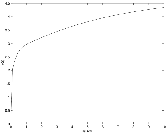
FIG. 1.: The momentum dependence of $n_{f}(Q^{2})$.

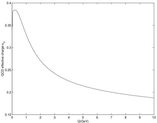
FIG. 2.: The effective charge ${\alpha}_{V}$, as given by Eqn. (3.16)

Note that in the beta function ${\beta}_{0}$ we use a “smeared” function for the number of flavors, although this only affects the low-energy regime where several quark flavor thresholds occur. This function is

$$n_{f}(Q^{2})=\sum_{f}\int_{0}^{1}dz\frac{6Q^{2}z^{2}(1-z)^{2}}{m_{f}^{2}+Q^{2}z(1-z)}\;,$$ (39)

and is motivated in Ref. [15]. The integration over $z$ in Eqn. (3.17) leads to the explicit representation of the function that is identical to the $Q^{2}$ logarithmic derivative of the one-loop massive $\beta$-function presented in Ref. [15]. In Fig. 1 we show $n_{f}(Q^{2})$ in the low-energy region. We have taken $m_{s}=0.15~{}{\rm GeV}$, $m_{c}=1.9~{}{\rm GeV}$, $m_{b}=4.5~{}{\rm GeV}$ for the quark masses. The resulting $\alpha_{V}$ is shown in Fig. 2.

Note also that for low $Q^{2}$ the couplings, although frozen, are large. Thus the NLO and higher-order terms in the CSRs are large, and they do not give accurate results at low scales. In addition, higher-twist contributions to the effective charges, which are not reflected in CSRs relating them, may be expected to be important for low $Q^{2}$. However, series expansions in terms of physical charges are likely to be more convergent than those cast in terms of unphysical couplings such as $\alpha_{\overline{MS}}$, which is singular at finite scales. Thus it is quite possible that expansions of the type we are considering can be extended to lower physical scales than series written in terms of $\alpha_{\overline{MS}}$. In any case, we will not be directly concerned with the low-$Q^{2}$ regime here.

Before discussing the results, it is useful to understand what improvements we can expect from the commensurate scale relations. First of all, of course, we have a scale-independent result, so aesthetically we have an advantage over the conventional treatment. Moreover, because of this we expect our result to be numerically more accurate than previous results with the scale fixed to certain value. The main applicability and usefulness of commensurate scale relations is for the intermediate energy regime. Pertubation theory is valid only above the characteristic QCD scale ${\Lambda}_{QCD}$, and since the commensurate scale analysis crucially depends on the validity of perturbation theory, we don’t expect much improvement in the very low energy regime. Furthermore, in the high energy limit the residual scale dependent terms go to zero, so scale relations are meaningless. The $e^{+}e^{-}$ annihilation data, as well as the Bjorken sum rule data presented in the next section, lies in the intermediate energy regime where we expect improved predictions.

Two additional modifications of Eqn. (30) were performed before comparing with data. First, we have included the leading-order electroweak corrections to account for the $Z^{0}$ current, which is particularly important above 30 GeV. In addition we have included the charm and bottom mass corrections, which are important in the range 3–15 GeV. The effect of these modifications is to replace the factor $\sum_{q}{e_{q}^{2}}$ in Eqn. (9) by

$$\sum_{q}\sqrt{1-\frac{4m_{q}^{2}}{Q^{2}}}\Biggl{[}e_{q}^{2}\left(1+\frac{2m_{q}^{2}}{Q^{2}}\right) + 2{\rm Re({\it r})}e_{q}c_{V}^{e}c_{V}^{q}\left(1+\frac{2m_{q}^{2}}{Q^{2}}\right)$$ (40)

$$+ |r|^{2}\left((c_{V}^{e})^{2}+(c_{A}^{e})^{2}\right)\left((c_{V}^{q})^{2}\left(1+\frac{2m_{q}^{2}}{Q^{2}}\right)+(c_{A}^{q})^{2}\left(1-\frac{4m_{q}^{2}}{Q^{2}}\right)\right)\Biggl{]}\;,$$ (41)

where

$$c_{V}^{q} = I_{3}-2{e_{q}}{\sin}^{2}{\theta}_{W}\;,$$ (42)

$$c_{V}^{e} = 2{\sin}^{2}{\theta}_{W}-\frac{1}{2}\;,$$ (43)

$$c_{A}^{q} = I_{3}\;,$$ (44)

$$c_{A}^{e} = -\frac{1}{2}\;,$$ (45)

$$r = \frac{\sqrt{2}GM_{Z}^{2}}{Q^{2}-M_{Z}^{2}+iM_{Z}{\Gamma}_{Z}}\left(\frac{Q^{2}}{e^{2}}\right)\;$$ (46)

$$= \frac{Q^{2}}{{\sin}^{2}{2{\theta}_{W}}(Q^{2}-M_{Z}^{2}+iM_{Z}{\Gamma}_{Z})}\;.$$ (47)

Here $I_{3}$ is the third component of the weak isospin of the quark coupled to $Z^{0}$ and the weak mixing angle $\theta_{W}$ is given by ${\sin}^{2}{\theta}_{W}=0.22$. The mass and the decay width of $Z^{0}$ are given by $M_{Z}=91.2~{}\rm{GeV}$ and ${\Gamma}_{Z}=2.5~{}\rm{GeV}$, respectively.

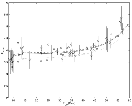
FIG. 3.: The scale-commensurate expansion of $\alpha_{R}$ in terms of $\alpha_{V}$ in the high energy regime. The solid line is given by Eqn. (3.11); the dashed line is the prediction quoted by the PDG; the dotted line is the leading order result (with mass and electroweak corrections).

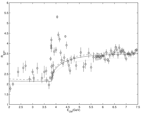
FIG. 4.: Scale-commensurate expansion of $\alpha_{R}$ in terms of $\alpha_{V}$ in the intermediate-energy regime.

In Fig. 3, we show the commensurate scale result (30) along with a representative subset of the available data [16] in the energy range 8–60 GeV. We find our results to be in excellent agreement with the data, as well as the standard QCD predictions quoted by the Particle Data Group [17] with the scale fixed to a certain value ($\Lambda_{\overline{MS}}=0.25\rm{GeV}$). In Fig. 4, we show our theoretical prediction and the data in the 2–7.5 GeV range. Again, we find very nice agreement with the data, particularly considering that we have neglected corrections from the $J/{\psi}(1S)$, ${\psi}(2S)$, and other vector meson resonances. Note that the data for $3.6~{}\rm{GeV}<Q<7.5~{}\rm{GeV}$ has been subtracted by $0.84\sqrt{1-{4m_{\tau}^{2}}/{Q^{2}}}\left(1+{2m_{\tau}^{2}}/{Q^{2}}\right)$ to account for hadronic production that proceeds via tau lepton pairs, which the early experiments did not distinguish from quark-hadron processes. The factor $0.84=1-(2/5)^{2}$ is the probability that either tau will decay to hadrons.

C Bjorken Sum Rule

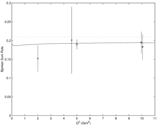
FIG. 5.: The dotted line shows the leading-order prediction for the Bjorken sum rule while the solid line includes the scale-commensurate corrections through NNLO. Also shown are data from Ref. [18] (crosses), from the E154 Collaboration [19] (circles), and from the SMC Collaboration [20] (stars).

Finally we present the scale-commensurate expansion of the Bjorken sum rule in terms of $\alpha_{V}$ at NNLO. The result is

$$\frac{{\alpha}_{g_{1}}(Q)}{\pi}=\frac{{\alpha}_{V}(Q_{g}^{*})}{\pi}+A_{g}\left(\frac{{\alpha}_{V}(Q_{g}^{**})}{\pi}\right)^{2}+B_{g}\left(\frac{{\alpha}_{V}(Q_{g}^{**})}{\pi}\right)^{3}+{\cdots}\;,$$ (48)

where

$$A_{g} = \frac{13}{12}$$ (49)

$$B_{g} = -\frac{131}{72}-\frac{27}{8}{\pi}^{2}+\frac{9}{64}{\pi}^{4}$$ (51)

$$\ln(Q_{g}^{*}/Q) = -\frac{1}{6}-\frac{43}{144}\left(11-\frac{2}{3}n_{f}\right)\left(\frac{{\alpha}_{V}(Q)}{\pi}\right)$$ (53)

$$\ln(Q_{g}^{**}/Q) = -\frac{191}{117}-\frac{5}{78}{\zeta}_{3}+\frac{30}{13}{\zeta}_{5}\;.$$ (55)

In Fig. 5 we show the commensurate scale result to NNLO and the leading order perturbative result with the five currently available data points. This plot strongly suggests that the higher order pQCD corrections do indeed give the correct convergence to the physical result. Our results may also be compared with an analysis of the Bjorken sum rule [10] using so-called analytic perturbation theory (APT) [21]. In Ref. [10], the authors show that by requiring the QCD coupling ${\alpha}_{s}$ to be analytic, thereby removing unphysical singularities, they can obtain approximately scheme independent results. Their plot of the correction to the Bjorken sum rule, $\alpha_{g_{1}}/\pi$, is very similar to what we obtain using commensurate scale relations.

IV Conclusions

In this paper, we have applied the physical QCD effective charge ${\alpha}_{V}$, defined by the heavy quark potential, in calculations of the $e^{+}e^{-}$ annihilation cross section and the Bjorken sum rule. Following the BLM procedure, we derived the NNLO scale-commensurate expansions of ${\alpha}_{R}$ and ${\alpha}_{g_{1}}$ in terms of ${\alpha}_{V}$ and used these expansions to numerically compute the $e^{+}e^{-}$ annihilation cross section and the Bjorken sum rule. Using a phenomenological form for the effective charge ${\alpha}_{V}$ [Eqn. (38)] which is consistent with the lattice determination of the heavy quark potential, we obtain excellent agreement between our results and the experimental data in both cases. Furthermore, because of the scale independence, we trust that our results are numerically more accurate than previous results with the scale fixed to a certain value. The application of scale-commensurate expansions to other observables is forthcoming.

- [1] S. J. Brodsky, G. P. Lepage, and P. B. Mackenzie, Phys. Rev. D 28, 228 (1983).
- [2] H. J. Lu and S. J. Brodsky, Phys. Rev. D 48, 3310 (1993).
- [3] S. J. Brodsky, G. T. Gabadadze, A. L. Kataev and H. J. Lu, Phys. Lett. 372B, 133 (1996).
- [4] M. Peter, Phys. Rev. Lett. 78, 602 (1997); Nucl. Phys. B 501, 471 (1997).
- [5] S. J. Brodsky and H. J. Lu, Phys. Rev. D 51, 3652 (1995).
- [6] H. J. Lu, Ph. D. thesis, Stanford University (1992).
- [7] E. C. G. Stückelberg and A. Peterman, Helv. Phys. Acta 26, 449 (1953); A. Peterman, Phys. Rept. 53C, 157 (1979).
- [8] S. G. Gorishny, A. L. Kataev and S. A. Larin, Phys. Lett. 259B, 144 (1991); L. R. Surguladze and M. A. Samuel, Phys. Rev. Lett 66, 560 (1991); ibid. 66, 2416(E) (1991); Phys. Lett. 309B, 157 (1993).
- [9] M. Anselmino, F. Caruso, and E. Levin, hep-ph/9505311; M. Anselmino, A. Efremov, and E. Leader, CERN preprint CERN-TH/7216/94.
- [10] K. A. Milton, I. L. Solovtsov and O. P. Solovtsova, hep-ph/9809510.
- [11] C. T. H. Davies, et al., Phys. Rev. D 52, 6519 (1995).
- [12] J. M. Cornwall, Phys. Rev. D 26, 1453 (1982).
- [13] S. J. Brodsky, C.-R. Ji, A. Pang and D. G. Robertson, Phys. Rev. D 57, 245 (1997).
- [14] A. C. Mattingly and P. M. Stevenson, Phys. Rev. D 49, 437 (1994).
- [15] D. V. Shirkov and S. V. Mikhailov, Z. Phys. C 63 463 (1994).
- [16] C. Caso et al., The European Physical Journal C 3, 1 (1998).
- [17] M. Dine and J. Sapirstein, Phys. Rev. Lett. 43, 668 (1979).
- [18] B. Adeva, et al., Phys. Lett. 302B, 533 (1993); ibid. 320B, 400 (1994); D. L. Anthony, et al., Phys. Rev. Lett. 71, 759 (1993).
- [19] K. Abe, et al. (E154 Collaboration), Phys. Lett. 405B, 180 (1997).
- [20] A. Adams, et al. (SMC Collaboration), Phys. Lett. 396B, 338 (1997); Phys. Rev. D 56, 5330 (1997); Phys. Lett. 412B, 414 (1997).
- [21] D. V. Shirkov and I. L. Solovtsov, JINR Rap. Comm. No. 2[76]-96, 5 (1996); hep-ph/9604363; Phys. Rev. Lett. 79, 1209 (1997).