Impact of $D^{0}-\overline{D^{0}}$ mixing on
the experimental determination of $\gamma$

Abstract

Several methods have been devised to measure the weak phase $\gamma$ using decays of the type $B^{\pm}\rightarrow DK^{\pm}$, where it is assumed that there is no mixing in the $D^{0}-\overline{D^{0}}$ system. However, when using these methods to uncover new physics, one must entertain the real possibility that the measurements are affected by new physics effects in the $D^{0}-\overline{D^{0}}$ system. We show that even values of $x_{D}$ and/or $y_{D}$ around $10^{-2}$ can have a significant impact in the measurement of $\sin^{2}{\gamma}$. We discuss the errors incurred in neglecting this effect, how the effect can be checked, and how to include it in the analysis.

I Introduction

In the next few years, the SM description of the charged current interactions through the Cabibbo–Kobayashi–Maskawa (CKM) matrix [1], and, in particular, the nature of CP violation, will be subject to tests of unprecedented precision. The final objective is to over-constrain the CKM matrix and, thus, probe any effects due to new physics. Two important tests will be the determination of $\sin(2\beta)$ from the CP violating asymmetry in $B_{d}\rightarrow J/\psi K_{S}$, where $\beta=\arg{\left(-V_{cd}V_{cb}^{\ast}/V_{td}V_{tb}^{\ast}\right)}$, and the search for $B^{0}_{s}-\overline{B^{0}_{s}}$ mixing.

Interesting constraints will also arise from the decay chains $B^{\pm}\rightarrow DK^{\pm}\rightarrow f_{D}K^{\pm}$. The idea here is based on the fact that

$$\frac{A(B^{+}\rightarrow D^{0}K^{+})}{A(B^{+}\rightarrow\overline{D^{0}}K^{+})}\sim\frac{V_{ub}^{\ast}V_{cs}}{V_{cb}^{\ast}V_{us}}\frac{a_{2}}{a_{1}}.$$ (1)

If the final state $f_{D}$ is common to $D^{0}$ and $\overline{D^{0}}$, then these two amplitudes interfere and one probes essentially the weak phase $\gamma=\arg{\left(-V_{ud}V_{ub}^{\ast}/V_{cd}V_{cb}^{\ast}\right)}$. The phenomenological factor $|a_{2}/a_{1}|\sim 0.26$ [2] accounts for the fact that the $B^{+}\rightarrow D^{0}K^{+}$ decay is color suppressed, while the $B^{+}\rightarrow\overline{D^{0}}K^{+}$ decay is not.

Inspired by a triangular construction due to Gronau and London [3], Gronau and Wyler (GW) proposed a method to extract $\sin^{2}\gamma$ which uses the decay chains $B^{\pm}\rightarrow DK^{\pm}\rightarrow f_{\rm cp}K^{\pm}$, where $f_{\rm cp}$ is a CP eigenstate [4]. Atwood, Dunietz, and Soni (ADS) have modified this method, using only final states $f_{D}$ which are not CP eigenstates [5]. Recently, Soffer has stressed the experimental advantages of combining the two strategies into a single analysis, while pointing out the complications due to the discrete ambiguities inherent in these methods and other measurements of direct CP violation [6].

The nice feature of these decays is that they involve only tree level diagrams and, thus, are not subject to penguin pollution. However, one must consider what effects the mixing in the $D^{0}-\overline{D^{0}}$ system might have on the $B^{\pm}\rightarrow DK^{\pm}\rightarrow f_{D}K^{\pm}$ decay chains [7], especially if these measurements are used to uncover new physics. Otherwise, new physics effects in the $D^{0}-\overline{D^{0}}$ system could be misidentified as new physics in the $B_{d}$ system. In fact, Meca and Silva [7] have used $x_{D}\sim 10^{-2}$ to argue that these effects could be of order $10\%$ in $B^{\pm}\rightarrow f_{D}K^{\pm}$ decays, and they may be as large as $100\%$ in $B^{\pm}\rightarrow f_{D}\rho^{\pm}$ or $B^{\pm}\rightarrow f_{D}\pi^{\pm}$ decays [8].

The main objective of our article is to study in detail the effect of $D^{0}-\overline{D^{0}}$ mixing on the measurement of $\gamma$ in $B^{\pm}\rightarrow DX^{\pm}$ decays. If $D^{0}-\overline{D^{0}}$ mixing is observed, it must be incorporated into the $B^{\pm}\rightarrow DX^{\pm}$ analysis. If only upper limits on mixing are known, their effect should be included as a systematic error. We also mention briefly how the effect of $D^{0}-\overline{D^{0}}$ mixing may, under certain conditions, be detected in the measurement of $\gamma$.

In section II we establish our notation. In section III we present the complete expressions for the $B^{\pm}\rightarrow DX^{\pm}\rightarrow f_{D}X^{\pm}$ decay rates in the presence of $D^{0}-\overline{D^{0}}$ mixing. In section IV, we start by studying the influence of $D^{0}-\overline{D^{0}}$ mixing on the GW and ADS methods separately, concentrating on some regions of parameter space. We show that these effects depend on the specific value of $\gamma$ and that they might affect the extraction of $\sin^{2}\gamma$ by as much as $75\%$, even for values of $x_{D}$ and/or $y_{D}$ around $10^{-2}$. Then, we combine the GW and ADS methods into a realistic experimental analysis, performing a scan over parameter space to discuss the impact that the mixing effects have on such experiments. We also show how to include the mixing effects in the analysis. We draw our conclusions in section V. For completeness, the formulae relevant for the study of the $D^{0}-\overline{D^{0}}$ system are included in appendix A. Appendix B contains a comparison between CP-even and CP-odd corrections to the extraction of $\sin^{2}\gamma$. Appendix C presents an analysis of the measurements of the strong phases in the $D$ decays that enter in the extraction of $\gamma$, and which may be performed at the tau-charm factories.

II Assumptions and notation

A Parametrizations of the decay amplitudes

One might be surprised by the fact that Eq. (1), is not invariant under the rephasing of the $u$ and $c$ quarks. In fact, the ratio measured experimentally in the GW and ADS methods is rather

$$\frac{A(B^{+}\rightarrow D^{0}K^{+})\,A(D^{0}\rightarrow f_{D})}{A(B^{+}\rightarrow\overline{D^{0}}K^{+})\,A(\overline{D^{0}}\rightarrow f_{D})}.$$ (2)

This ratio depends on the weak phase in Eq. (1), on the relative weak phase between the decay amplitudes $A(D^{0}\rightarrow f_{D})$ and $A(\overline{D^{0}}\rightarrow f_{D})$, and it has the correct rephasing-invariant properties. The weak phase in Eq. (2) is essentially given by $\gamma$. Indeed, tree level, $W$-mediated $D$ decays only probe the weak phase in the first two families, $\chi^{\prime}=\arg{\left(-V_{us}V_{ud}^{\ast}/V_{cs}V_{cd}^{\ast}\right)}$, and this is also the weak phase that appears with $\gamma$ in Eq. (1). In the SM, $\chi^{\prime}$ lies around $0.003$ radians [9] and its presence is completely irrelevant. New physics could, in principle, affect this result by altering $\chi^{\prime}$ or by allowing for new diagrams to drive the $D$ decays. However, both $\chi^{\prime}$ [10] and any additional contributions to $D$ decays [11] are likely to remain small in most models of new physics. We will neglect them henceforth.

For simplicity, we will use the parametrizations

$$A(B^{+}\rightarrow\overline{D^{0}}K^{+})=B, A(B^{+}\rightarrow D^{0}K^{+})=\tilde{\epsilon}\,B\,e^{i\gamma}e^{i\Delta_{B}},$$ (3)

$$A(B^{-}\rightarrow D^{0}K^{-})=B, A(B^{-}\rightarrow\overline{D^{0}}K^{-})=\tilde{\epsilon}\,B\,e^{-i\gamma}e^{i\Delta_{B}}\ ,$$ (4)

for the initial $B^{\pm}$ decays;

$$A(\overline{D^{0}}\rightarrow K^{+}\pi^{-})=A(D^{0}\rightarrow K^{-}\pi^{+}) = A,$$ (5)

$$A(D^{0}\rightarrow K^{+}\pi^{-})=A(\overline{D^{0}}\rightarrow K^{-}\pi^{+}) = -\epsilon\,A\,e^{i\Delta_{D}},$$ (6)

for the $D$ decays into non-CP eigenstates; and

$$A(D^{0}\rightarrow f_{\rm cp})=A_{\rm cp},\ \ \ A(\overline{D^{0}}\rightarrow f_{\rm cp})=\eta_{f}A_{\rm cp},$$ (7)

for $D$ decays into a CP eigenstate $f_{\rm cp}$ with CP eigenvalue $\eta_{f}$. In these parametrizations, we have removed all irrelevant overall CP-even phases. However, the differences between CP-even phases in competing paths, $\Delta_{B}$ and $\Delta_{D}$, are physically meaningful. $\epsilon$ and $\tilde{\epsilon}$ are discussed in the next section.

B Estimates of the parameters

In the SM, the value of $\gamma$ is already constrained by an overall analysis of the unitarity triangle. In recent reviews Ali and London find [12]

$$36^{\circ}\leq\gamma\leq 97^{\circ}\ \ \ \Longrightarrow\ \ \ 0.35\leq\sin^{2}\gamma\leq 1.00\ ,$$ (8)

while Buras [13] quotes $44^{\circ}\leq\gamma\leq 97^{\circ}$. The variations found in the literature are mostly due to different estimates for the theoretical errors and to the different methods used to combine the theoretical and experimental errors. For definiteness, we will use Eq. (8) as a reasonable estimate for the allowed region in the SM. However, we stress that $\gamma$ is allowed to take any value in our analysis. We are concerned not only with the effects that $D^{0}-\overline{D^{0}}$ mixing may have on SM values of $\gamma$, but also with the possibility that such mixing effects may ‘hide’ new-physics by bringing values of $\gamma$ outside the SM allowed region into this region.

Using $|V_{ub}/V_{cb}|\sim 0.08$ [14], Eq. (1), and assuming factorization, we get

$$\tilde{\epsilon}\sim|V_{ub}^{\ast}V_{cs}/V_{cb}^{\ast}V_{us}|\,|a_{2}/a_{1}|\sim 0.09\ .$$ (9)

Notice that the parametrization in Eq. (4) is valid for any $B^{+}\rightarrow DX^{+}$ decay, with $X^{+}=K^{+},\pi^{+},\rho^{+}$, and higher resonances, but the exact values of $B$, $\tilde{\epsilon}$ and $\Delta_{B}$ will vary from one channel to the next. For example, for the $B^{+}\rightarrow D\pi^{+}$ and $B^{+}\rightarrow D\rho^{+}$ decays we expect

$$\tilde{\epsilon}_{\pi}\sim|V_{ub}^{\ast}V_{cd}/V_{cb}^{\ast}V_{ud}|\,|a_{2}/a_{1}|\sim 0.09\times(0.22)^{2}\sim 0.004.$$ (10)

In addition, ${\cal B}[B^{+}\rightarrow\overline{D^{0}}\rho^{+}]=(1.34\pm 0.18)\times 10^{-2}$, ${\cal B}[B^{+}\rightarrow\overline{D^{0}}\pi^{+}]=(5.3\pm 0.5)\times 10^{-3}$ [15], and ${\cal B}[B^{+}\rightarrow\overline{D^{0}}K^{+}]/{\cal B}[B^{+}\rightarrow\overline{D^{0}}\pi^{+}]=0.055\pm 0.015$ [16]. While the factor $B^{2}$ is roughly $18$ ($46$) times larger in $B^{+}\rightarrow D\pi^{+}$ ($B^{+}\rightarrow D\rho^{+}$) decays than it is in $B^{+}\rightarrow DK^{+}$ decays, the decay chains of interest to us will scale instead with the $B^{2}\tilde{\epsilon}^{2}$ factors in the CKM-suppressed decays

$${\cal B}[B^{+}\rightarrow D^{0}K^{+}] \sim \tilde{\epsilon}^{2}\ {\cal B}[B^{+}\rightarrow\overline{D^{0}}K^{+}]\sim 2.4\times 10^{-6},$$ (11)

$${\cal B}[B^{+}\rightarrow D^{0}\pi^{+}] \sim \tilde{\epsilon}_{\pi}^{2}\ {\cal B}[B^{+}\rightarrow\overline{D^{0}}\pi^{+}]\sim 1.0\times 10^{-7},$$ (12)

$${\cal B}[B^{+}\rightarrow D^{0}\rho^{+}] \sim \tilde{\epsilon}_{\pi}^{2}\ {\cal B}[B^{+}\rightarrow\overline{D^{0}}\rho^{+}]\sim 2.5\times 10^{-7}.$$ (13)

As a result, the $B^{+}\rightarrow DK^{+}$ decays are the best to extract $\sin^{2}\gamma$.

Similarly, for the decays used in the ADS method, $\epsilon$ is the magnitude of the ratio of the amplitudes of the doubly Cabibbo suppressed (DCS) decay $\overline{D^{0}}\rightarrow K^{-}\pi^{+}$ to the Cabibbo allowed (CA) decay $D^{0}\rightarrow K^{-}\pi^{+}$. This may be estimated from [17]

$$\epsilon\sim\sqrt{\frac{{\cal B}[\overline{D^{0}}\rightarrow K^{-}\pi^{+}]}{{\cal B}[D^{0}\rightarrow K^{-}\pi^{+}]}}\sim\sqrt{0.0031}\sim 0.06\ .$$ (14)

The parametrization in Eq. (6) is valid for any $D\rightarrow f_{D}$ decay, but the exact values of $A$, $\epsilon$ and $\Delta_{D}$ will vary from one channel to the next. In particular, Eq. (6) reduces to Eq. (7) when $\Delta_{D}=0$ and $-\epsilon=\eta_{f}=\pm 1$ is the CP eigenvalue of $f_{\rm cp}$. For the CP-even eigenstates, such as $K^{+}K^{-}$ and $\pi^{+}\pi^{-}$, $\epsilon=-1$. For the CP-odd eigenstates, such as $K_{S}\pi^{0}$ and $K_{S}\phi$, $\epsilon=+1$.

The mixing in the $D^{0}-\overline{D^{0}}$ system may be parametrized by the mass difference divided by the average width ($x_{D}\equiv\Delta m/\Gamma$), by the width difference divided by twice the average width ($y_{D}\equiv\Delta\Gamma/(2\Gamma)$), and by a CP-violating phase ($\theta_{D}$) defined by $q_{D}/p_{D}=e^{2i\theta_{D}}$. Assuming $\theta_{D}=0$,

$$x_{D}^{2}+y_{D}^{2}\leq\left(6.7\times 10^{-2}\right)^{2},$$ (15)

at the $95\%$ C. L. [18]. This bound is likely to remain stable even when one allows for $\theta_{D}\neq 0$ [19].

Predictions for $x_{D}$ and $y_{D}$ within the SM vary considerably among the different authors [20], but it is probably safe to estimate an upper bound around a few times $10^{-3}$. This uncertainty is due to the role played by SU(3) breaking effects in the long-distance part of the calculation. For example, Bucella, Lusignoli and Pugliese [21] have estimated the SM value for $y_{D}$ to lie around $1.5\times 10^{-3}$. However, this result might be subject to sizeable errors, since it comes about through a large cancellation between two individual contributions, each of order $3\times 10^{-2}$. On the other hand, in the SM, the value of $\theta_{D}$ is related to $\chi^{\prime}$ and is guaranteed to be extremely small.

When one goes beyond the SM, one finds many models for which $\theta_{D}$ may be large and $x_{D}\sim 10^{-2}$, while $y_{D}$ (which is closely related to the decay rates, where one would hardly expect any large new physics contributions) is likely to retain its (rather uncertain) SM value [20]. Ultimately, these values will be determined experimentally at $B$-factories, in fixed target experiments, and at tau-charm factories. We take the point of view that, until a determination of $x_{D}$ and $y_{D}$ is available, their upper bounds must be included as a systematic uncertainty in the experimental determination of $\gamma$ from the $B^{\pm}\rightarrow DK^{\pm}$ decays.

The relevant point about the notation introduced here is that $\epsilon$ and $\tilde{\epsilon}$ are of order $10^{-1}$, while we will take $x_{D}\sim y_{D}\sim 10^{-2}$ as an illustrative example. (This is of the order of the sensitivity expected in the near future [22].) Therefore, any effect proportional to $x_{D}/\tilde{\epsilon}$, $y_{D}/\tilde{\epsilon}$, $x_{D}/\epsilon$, or $y_{D}/\epsilon$ is naturally of order $10\%$ [7], and might be larger depending on the exact value of the other parameters in the problem.

We should stress that the $D^{0}-\overline{D^{0}}$ mixing effects might be of order unity, or even dominate, in the $B^{\pm}\rightarrow D\pi^{\pm}$ and $B^{\pm}\rightarrow D\rho^{\pm}$ decays, because $\tilde{\epsilon}_{\pi}\sim 0.004$ [8]. As a result, even SM values around $x_{D}\sim y_{D}\sim 10^{-3}$, would lead to a $10\%$ effect in these channels [8].

III The $B^{\pm}\rightarrow DK^{\pm}\rightarrow f_{D}K^{\pm}$ decay rates

FIG. 1.: The $B^{\pm}\rightarrow DK^{\pm}\rightarrow f_{D}K^{\pm}$ decay chain, specified for the case of $f_{D}=K^{-}\pi^{+}$. For a CP eigenstate $f_{D}=f_{\rm cp}$ one just needs to take $\epsilon=\pm 1$.

The $B^{+}\rightarrow DK^{+}\rightarrow f_{D}K^{+}$ decay chain is shown in Fig. 1. The solid lines refer to decays and the dashed lines to the time evolution of the $D^{0}-\overline{D^{0}}$ system. The functions $g_{+}(t)$ and $g_{-}(t)$ are discussed in appendix A and describe the flavor preserving and flavor changing time evolutions, respectively. The corresponding decay amplitude is obtained simply by adding the four possible decay paths

$$A\left(B^{+}\rightarrow DK^{+}\rightarrow f_{D}K^{+}\right) = A(B^{+}\rightarrow\overline{D^{0}}K^{+})\ g_{+}(t)\ A(\overline{D^{0}}\rightarrow f_{D})$$ (16)

$$+ A(B^{+}\rightarrow D^{0}K^{+})\ g_{+}(t)\ A(D^{0}\rightarrow f_{D})$$ (17)

$$+ A(B^{+}\rightarrow\overline{D^{0}}K^{+})\ \frac{p_{D}}{q_{D}}\,g_{-}(t)\ A(D^{0}\rightarrow f_{D})$$ (18)

$$+ A(B^{+}\rightarrow D^{0}K^{+})\ \frac{q_{D}}{p_{D}}\,g_{-}(t)\ A(\overline{D^{0}}\rightarrow f_{D}).$$ (19)

The magnitude squared of this expression yields the time dependent decay rate.

Using the notation of section II, we find,

$$\frac{1}{A^{2}B^{2}}\,\Gamma\left[B^{+}\rightarrow DK^{+}\rightarrow f_{D}K^{+}\right]=$$ (20)

$$\hskip 34.44434pt|g_{+}(t)|^{2}\ \left[\tilde{\epsilon}^{2}+\epsilon^{2}-2\epsilon\tilde{\epsilon}\cos(\gamma+\Delta_{B}-\Delta_{D})\right]$$ (21)

$$\hskip 25.83325pt+\ |g_{-}(t)|^{2}\ \left[1+\epsilon^{2}\tilde{\epsilon}^{2}-2\epsilon\tilde{\epsilon}\cos(\gamma+4\theta_{D}+\Delta_{B}+\Delta_{D})\right]$$ (22)

$$\hskip 25.83325pt+\ 2\,\mbox{Im}\left(g_{+}^{\ast}(t)g_{-}(t)\right)\ \left[\tilde{\epsilon}(1-\epsilon^{2})\sin(\gamma+2\theta_{D}+\Delta_{B})-\epsilon(1-\tilde{\epsilon}^{2})\sin(2\theta_{D}+\Delta_{D})\right]$$ (23)

$$\hskip 25.83325pt+\ 2\,\mbox{Re}\left(g_{+}^{\ast}(t)g_{-}(t)\right)\ \left[\tilde{\epsilon}(1+\epsilon^{2})\cos(\gamma+2\theta_{D}+\Delta_{B})-\epsilon(1+\tilde{\epsilon}^{2})\cos(2\theta_{D}+\Delta_{D})\right].$$ (24)

To obtain the expression for the CP-conjugated decay rate, $B^{-}\rightarrow DK^{-}\rightarrow\bar{f}_{D}K^{-}$, we simply substitute $\gamma\rightarrow-\gamma$ and $\theta_{D}\rightarrow-\theta_{D}$. As shown in appendix A, the time integrated decay rates may be obtained through the substitutions $|g_{\pm}(t)|^{2}\rightarrow G_{\pm}$ and $g_{+}^{\ast}(t)g_{-}(t)\rightarrow G_{+-}$.

These expressions are completely general; no approximations were made (except for the use of $|q/p|=1$). In subsequent derivations we will often simplify the expressions, using the fact that $x_{D}$, $y_{D}$, and $\tilde{\epsilon}$ are small when compared with one. However the plots and estimates presented in this article were calculated using the complete formulae. We will also expand in $\epsilon$, except for decays into CP-even (CP-odd) eigenstates, where $\epsilon=-1$ ($\epsilon=+1$), $\Delta_{D}=0$, and $A\rightarrow A_{\rm cp}$.

Eq. (24) exhibits the usual three types of CP-violating terms. The first line on the RHS contains a term proportional to $\sin{\gamma}\sin{\Delta_{B}}$, which is due to direct CP violation in the $B^{\pm}\rightarrow DK^{\pm}$ decays (and appears multiplied by $\cos\Delta_{D}$ in the full decay chain). The last line contains a term proportional to $\sin{(2\theta_{D})}\sin{\Delta_{D}}$, which is due to direct CP violation in the $D\rightarrow f_{D}$ decays. In both cases, CP violation requires a non-zero strong phase. The usual CP violation in $D^{0}-\overline{D^{0}}$ mixing has already been neglected in Eq. (24) due to the assumption that $|q_{D}/p_{D}|=1$. The third line on the RHS contains a term proportional to $\sin{(2\theta_{D})}\cos{\Delta_{D}}$. This term is due to the interference between the mixing in the $D^{0}-\overline{D^{0}}$ system and its subsequent decay into the final state $f_{D}$. This term is not zero even if the strong phase $\Delta_{D}$ vanishes, but it requires a nontrivial new phase in the mixing, $\theta_{D}$. We could name this a first-mix-then-decay type of interference CP violation.

In addition, Eq. (24) contains a fourth type of CP-violating term. This appears on the third line of Eq. (24) as the term involving $\sin{(\gamma+2\theta_{D})}\cos{\Delta_{B}}$. This term persists even if $\Delta_{B}=0$ (meaning that no strong phase is required), or/and $\theta_{D}=0$ (meaning that no new phase is required in $D^{0}-\overline{D^{0}}$ mixing). In fact, in the limit $\theta_{D}=\Delta_{D}=0$, this term is proportional to $\sin\gamma$ and, therefore, it is large even within the SM. This fourth type of CP violation was first pointed out by Meca and Silva [7], and it arises from the interference between the $B\rightarrow D$ decays and the subsequent $D^{0}-\overline{D^{0}}$ mixing. We might call this the first-decay-then-mix type of interference CP violation. Its effect is best highlighted by considering a final state $f_{D}$ which tags the flavor of the $D^{0}$ meson (corresponding to $\epsilon=0$ in Fig. 1). In that case Fig. 1 has only two paths and there is still CP violation proportional to $\sin\gamma$, meaning that it can be large even within the SM. This example should help in clearing some frequent misconceptions found in the literature. We see that

• one may in principle use a single charged $B$ decay (and its CP conjugate) to probe a source of CP violation which does not require strong phases, as long as a neutral $D$ meson system is present in the intermediate state;

• one can have a large CP-violating phase involving the $D^{0}-\overline{D^{0}}$ system, even within the SM. It is true that, in the SM, the CP-violating phases present in the $D^{0}-\overline{D^{0}}$ mixing and $D$ decays are very small, because they are proportional to $\chi^{\prime}$. However, there is a large CP-violating phase in the first-decay-then-mix type of interference CP violation involved in $B\rightarrow D$ decays, even within the SM;

• the first-decay-then-mix type of interference CP violation can, in principle, be probed even when the $D$ meson is detected through its (flavor-tagging) semileptonic decay.

In general these effects require values of $x_{D}$ and/or $y_{D}$ around $10^{-2}$, in order to have an impact on $B^{\pm}\rightarrow D^{0}K^{\pm}$ decays. Nevertheless, as we shall see below, some values of the parameters are possible for which $y_{D}\sim 10^{-2}$ would give a $75\%$ effect, meaning that $y_{D}\sim 10^{-3}$ would still give a $7\%$ effect.

IV The determination of $\gamma$ in the presence of $D^{0}-\overline{D^{0}}$ mixing

A The no-mixing approximation

If there were no mixing in the $D^{0}-\overline{D^{0}}$ system, then we would have $g_{+}(t)=e^{-\Gamma t/2}$ and $g_{-}(t)=0$, cf. appendix A. This would leave only the uppermost and lowermost (unmixed) decay paths of Fig. 1; the mixed paths represented by the diagonal dashed time-evolution lines would be absent. This is precisely what one assumes in both the GW and ADS methods. In that case, the decay amplitude reduces to the first two line of Eq. (19) and the only relevant phase is that in Eq. (2). As discussed above, the corresponding weak phase is essentially given by $\gamma$.

Obviously, under the no-mixing approximation, these decays are completely insensitive to any CP-violating phase $\theta_{D}$ that might be present in $D^{0}-\overline{D^{0}}$ mixing.

In the GW method, one uses time-integrated decays rates into CP-eigenstates, given by

$$\Gamma\left[B^{+}\rightarrow f_{\rm cp}K^{+}\right] \propto 1+\tilde{\epsilon}^{2}+2\tilde{\epsilon}\cos(\gamma+\Delta_{B}),$$ (25)

$$\Gamma\left[B^{-}\rightarrow f_{\rm cp}K^{-}\right] \propto 1+\tilde{\epsilon}^{2}+2\tilde{\epsilon}\cos(\gamma-\Delta_{B}).$$ (26)

Gronau and Wyler [4] assume that $A_{\rm cp}$, $B$, and $\tilde{\epsilon}$ are known from the decay rates of $D\rightarrow f_{\rm cp}$, $B^{+}\rightarrow\overline{D^{0}}K^{+}$, and $B^{+}\rightarrow D^{0}K^{+}$, respectively. Therefore, Eqs. (26) determine

$$c_{+}=\cos(\gamma+\Delta_{B}),\ \ \mbox{and}\ \ c_{-}=\cos(\gamma-\Delta_{B}),$$ (27)

from which one may extract,

$$\sin^{2}\gamma = \frac{1}{2}\left[1-c_{+}c_{-}\pm\sqrt{(1-c_{+}^{2})(1-c_{-}^{2})}\right],$$ (28)

$$\sin^{2}\Delta = \frac{1}{2}\left[1-c_{+}c_{-}\mp\sqrt{(1-c_{+}^{2})(1-c_{-}^{2})}\right].$$ (29)

As discussed below, this determines $\gamma$ up to an eight-fold ambiguity [6].

Unfortunately, the GW method is difficult to implement for two main reasons. The first reason is due to the hierarchy between the two interfering amplitudes presented in Eqs. (1) and (9). This is easily seen by noting that the GW method hinges on extracting an interference of order $\tilde{\epsilon}$ from an overall rate of order one, as shown in Eqs. (26). Since Eqs. (26) can be visualized as two triangles in the complex amplitude plane, this problem is sometimes explained by pointing out that the two triangles are squashed.

The second reason arises from the fact that it is very difficult to measure ${\cal B}[B^{+}\rightarrow D^{0}K^{+}]$ (and, thus, $\tilde{\epsilon}$) experimentally. One could envision determining ${\cal B}[B^{+}\rightarrow D^{0}K^{+}]$ through the unmixed semileptonic decay chain, $B^{+}\rightarrow D^{0}K^{+}\rightarrow(X^{-}l^{+}\nu_{l})_{D}K^{+}$. However, since full reconstruction is impossible in semileptonic decays, this process is subject to daunting combinatoric backgrounds. Therefore, one is led to probe ${\cal B}[B^{+}\rightarrow D^{0}K^{+}]$ through the subsequent decay of the $D^{0}$ into hadronic final states, such as $K^{-}\pi^{+}(n\pi)^{0}$. However, as pointed out by Atwood, Dunietz and Soni [5], the two (unmixed) decay chains, $B^{+}\rightarrow D^{0}K^{+}\rightarrow(K^{-}\pi^{+})_{D}K^{+}$ and $B^{+}\rightarrow\overline{D^{0}}K^{+}\rightarrow(K^{-}\pi^{+})_{D}K^{+}$ interfere at order one, since

$$\frac{A(B^{+}\rightarrow D^{0}K^{+})\,A(D^{0}\rightarrow K^{-}\pi^{+})}{A(B^{+}\rightarrow\overline{D^{0}}K^{+})\,A(\overline{D^{0}}\rightarrow K^{-}\pi^{+})}\sim\frac{\tilde{\epsilon}}{\epsilon}\sim 1.5\ .$$ (30)

This means that it is very difficult to determine $\tilde{\epsilon}$ and, thus, to implement the GW method.

Atwood, Dunietz and Soni [5], have turned this order one interference problem into an asset. In their method, one uses two final states $f_{D}$ for which $\overline{D^{0}}\rightarrow f_{D}$ is a DCS decay, while $D^{0}\rightarrow f_{D}$ is Cabibbo allowed. Examples include $f_{D}=K^{-}\pi^{+}$, $K^{-}\pi^{+}\pi^{0}$, $K^{-}\pi^{+}\pi^{-}\pi^{+}$, etc. Then, there are four decay rates,

$$\Gamma\left[B^{+}\rightarrow f_{Di}K^{+}\right] \propto \tilde{\epsilon}^{2}+\epsilon_{i}^{2}-2\tilde{\epsilon}\epsilon_{i}\cos(\gamma+\Delta_{B}-\Delta_{Di}),$$ (31)

$$\Gamma\left[B^{-}\rightarrow\bar{f}_{Di}K^{-}\right] \propto \tilde{\epsilon}^{2}+\epsilon_{i}^{2}-2\tilde{\epsilon}\epsilon_{i}\cos(\gamma-\Delta_{B}+\Delta_{Di}),$$ (32)

which may be solved for the four unknowns: $\tilde{\epsilon}$, $\gamma$, $\Delta_{B}-\Delta_{D1}$, and $\Delta_{B}-\Delta_{D2}$. For each final state, $i=1$ or $i=2$, one can use the analogue of Eq. (28) to obtain $\sin^{2}\gamma$ and $\sin^{2}(\Delta_{B}-\Delta_{Di})$. These expressions, of course, depend on the unknown $\tilde{\epsilon}$, which is determined (up to discrete ambiguities) by requiring that the expressions for $\sin^{2}\gamma$ found for $i=1$ and for $i=2$ match. Here, although the interference terms contribute at order $\tilde{\epsilon}\epsilon$, the other terms are $\tilde{\epsilon}^{2}$, and $\epsilon^{2}$. As a result, the interference is of order one, and the corresponding triangles in the complex amplitude plane are no longer squashed.

Soffer [6] has proposed to maximize the analyzing power of the analysis by combining the GW and ADS methods, allowing each of them to contribute the information it is most sensitive to. In this scheme, one measures $\tilde{\epsilon}$, $\Delta_{D}$, $\Delta_{B}$, and $\gamma$ by minimizing the function

$$\chi^{2}=\sum_{m={\rm ADS,GW}}\left({\Gamma^{th}_{m}-\Gamma^{exp}_{m}\over\sigma_{m}^{exp}}\right)^{2}+{\rm CP\ Conj}.$$ (33)

$\chi^{2}$ compares the measured integrated decay rates $\Gamma^{exp}_{m}$ in both the GW and ADS methods, with their theoretical expectations, $\Gamma_{m}^{th}$. $\Gamma_{m}^{th}$ are functions of $\tilde{\epsilon}$, $\Delta_{B}$, $\gamma$, and $\Delta_{D}$, as given by Eqs. (26) (for $m={\rm GW}$) and (32) (for $m={\rm ADS}$). The comparison is done with respect to the measurement uncertainties, $\sigma_{m}^{exp}$.

This analysis has several advantages over the individual GW and ADS methods, and, therefore, it is most likely to be used in the actual experiment. First, combining the relatively high-statistics GW modes with the small ADS decay rates improves the measurement sensitivity, due to the addition of independent data. Second, a single ADS mode is enough to measure all four unknowns, leaving other modes to add redundancy and statistics. Third, this analysis is useful in removing some discrete ambiguities, as discussed below.

B Discrete ambiguities

We will now discuss the discrete ambiguities involved in the determination of $\gamma$. We start by recalling that Eq. (28) determines $\gamma$ up to an eight-fold ambiguity [6]. A two-fold ambiguity arises from the fact that we know the signs of the cosines of $\gamma+\Delta_{B}$ and $\gamma-\Delta_{B}$, but not the signs of the corresponding sine functions. Physically, this amounts to a confusion between $\gamma$ and $\Delta_{B}$. A further four-fold ambiguity arises from the fact that a determination of $\sin^{2}\gamma$ only determines the angle $\gamma$ up to the four fold ambiguity $\gamma$, $\pi-\gamma$, $\pi+\gamma$, and $2\pi-\gamma$. Another way to interpret this ambiguity is to notice that Eqs. (26) are invariant under the three independent transformations [6]

$$S_{\rm sign} : \ \ \ \gamma\rightarrow-\gamma,\ \ \ \ \ \Delta_{B}\rightarrow-\Delta_{B};$$ (34)

$$S_{\rm exchange} : \ \ \ \gamma\longleftrightarrow\Delta_{B};$$ (35)

$$S_{\pi} : \ \ \ \gamma\rightarrow\gamma+\pi,\ \ \ \Delta_{B}\rightarrow\Delta_{B}-\pi.$$ (36)

These discrete ambiguities are present in both the GW and ADS decay rates[6]. The $S_{\rm exchange}$ symmetry is $\gamma\leftrightarrow\Delta_{B}$ for the GW decay rates, but $\gamma\leftrightarrow\Delta_{B}-\Delta_{D}$ for the ADS rates. Thus, by combining the two methods, the $S_{\rm exchange}$ ambiguity can be resolved with a single ADS mode, for which $\Delta_{D}$ is large enough. Large values of $\Delta_{D}$ are expected in the SM. By contrast, resolving the $S_{\rm exchange}$ ambiguity in the GW method, requires that $\Delta_{B}$ vary significantly from one $B$ decay mode to the other. This is unlikely, because the experimental limits on CP-conserving phases in $B\rightarrow D\pi$, $D^{*}\pi$, $D\rho$ and $D^{*}\rho$ [23] suggest that the $\Delta_{B}$ are small.

The $S_{\rm sign}$ and $S_{\pi}$ ambiguities are likely to degrade the value of the measurement of $\gamma$ in a non-discrete manner. This is due to the fact that, for $\gamma$ within the currently allowed region, Eq. (8), $S_{\rm sign}S_{\pi}\gamma$ tends to be close enough to $\gamma$ to make the two values indistinguishable within the experimental errors. Overall, this results in a broad dip in the $\chi^{2}$ of Eq. (33) as a function of the measured value of $\gamma$, which is likely to substantially increase the measurement uncertainty [6].

It is therefore instructive to notice that the term $\sin(\gamma+2\theta_{D}+\Delta_{B})$ of Eq. (24) breaks the $S_{\rm sign}$ symmetry. As a result, one could naively expect that, incorporating mixing into the analysis would resolve the $S_{\rm sign}$ ambiguity and hence the $S_{\rm sign}S_{\pi}$ ambiguity, bringing about significant improvement over the no-mixing case.

Unfortunately, the $S_{\rm sign}$-breaking term is too small to have a significant effect with foreseeable data sample sizes. This term vanishes in the large GW modes, in which $f_{D}=f_{\rm cp}$, and it accounts for about 10% of the rate in the ADS modes when $x_{D}=0.01$. It is estimated [6] that with 600 fb^-1 collected at a next-generation B factory, the number of events in the ADS modes may be as large as 130. The $S_{\rm sign}$ violating term thus accounts for some 13 events, and its contribution to the $\chi^{2}$ is only about $(13/\sqrt{130})^{2}=1.3$, even when background is neglected. Therefore, we conclude that 60 times more data are needed to effectively resolve the $S_{\rm sign}$ ambiguity at the $\chi^{2}=10$ level.

C The GW decay rates in the presence of mixing

In the presence of $D^{0}-\overline{D^{0}}$ mixing, the $B^{+}\rightarrow DK^{+}\rightarrow f_{\rm cp}K^{+}$ decay rates involved in the GW method are altered according to Eq. (24). We find,

$$\Gamma\left[B^{+}\rightarrow f_{\rm cp}K^{+}\right] \propto 1+\tilde{\epsilon}^{2}+2\eta_{f}\,\tilde{\epsilon}\cos(\gamma+\Delta_{B})$$ (38)

$$-\eta_{f}\,x_{D}\sin(2\theta_{D})-y_{D}\left[2\tilde{\epsilon}\cos{(\gamma+2\theta_{D}+\Delta_{B})}+\eta_{f}\,\cos{(2\theta_{D})}\right],$$

$$\Gamma\left[B^{-}\rightarrow f_{\rm cp}K^{-}\right] \propto 1+\tilde{\epsilon}^{2}+2\eta_{f}\,\tilde{\epsilon}\cos(\gamma-\Delta_{B})$$ (40)

$$+\eta_{f}\,x_{D}\sin(2\theta_{D})-y_{D}\left[2\tilde{\epsilon}\cos{(\gamma+2\theta_{D}-\Delta_{B})}+\eta_{f}\,\cos{(2\theta_{D})}\right],$$

to linear order in $x_{D}$ and $y_{D}$. Recall that $\eta_{f}=\pm 1$ is the CP eigenvalue of the CP eigenstate $f_{\rm cp}$.

In these expressions we have effectively dropped the last line of Eq. (19), because the corresponding decay chain is suppressed both by $\tilde{\epsilon}$ and by $D^{0}-\overline{D^{0}}$ mixing. Moreover, since we are only keeping linear terms in $x_{D}$ and $y_{D}$, the second line of Eq. (24) does not contribute. These approximations were made in order to simplify the expressions. We stress that we have used the full expressions in our analysis and in all the computer simulations.

The crucial step in the GW method is the identification of the interference terms on the first lines of Eqs. (40): $\cos(\gamma\pm\Delta_{B})$. These are identified with $c_{\pm}$ in Eqs. (27), which are then used in Eq. (28). In the GW method this interference is of order $\tilde{\epsilon}$ (although it is buried in an overall decay rate of order one), while the leading mixing contributions are of order $x_{D}$ and $y_{D}$. Taking $x_{D}\sim y_{D}\sim 10^{-2}$, we expect the corrections to the determination of $\sin^{2}\gamma$ to be of order $x_{D}/\tilde{\epsilon}\sim y_{D}/\tilde{\epsilon}\sim 10^{-1}$.

It is clear that the importance of the mixing terms depends on the exact values of $\gamma$ and $\Delta_{B}$. Therefore, they could be much larger than the previous naive estimate might lead us to believe. Similar considerations apply to the ADS method. As long as only upper bounds on $D^{0}-\overline{D^{0}}$ mixing are known, these effects constitute systematic uncertainties that must be added to any other experimental uncertainties.

If there is $D^{0}-\overline{D^{0}}$ mixing, but this is ignored in the experimental analysis, then the $c_{\pm}$ extracted from the GW method become

$$c_{+w} = \cos(\gamma+\Delta_{B})-\frac{x_{D}}{2\tilde{\epsilon}}\sin(2\theta_{D})-\frac{y_{D}}{2\tilde{\epsilon}}\left[2\eta_{f}\,\tilde{\epsilon}\cos{(\gamma+2\theta_{D}+\Delta_{B})}+\cos{(2\theta_{D})}\right],$$ (41)

$$c_{-w} = \cos(\gamma-\Delta_{B})+\frac{x_{D}}{2\tilde{\epsilon}}\sin(2\theta_{D})-\frac{y_{D}}{2\tilde{\epsilon}}\left[2\tilde{\epsilon}\eta_{f}\,\cos{(\gamma+2\theta_{D}-\Delta_{B})}+\cos{(2\theta_{D})}\right],$$ (42)

to linear order in $x_{D}$ and $y_{D}$. The $x_{D}$ terms are only important if there is also a large new CP-violating phase $\theta_{D}$ in the $D^{0}-\overline{D^{0}}$ mixing. In contrast, the second $y_{D}$ term is important even if $\theta_{D}$ is small. This is closely related to the fact that the linear term in the time-dependent expression for the direct $D\rightarrow f_{\rm cp}$ decays is proportional to $y_{D}\cos{(2\theta_{D})}\pm x_{D}\sin(2\theta_{D})$ [24]. When Eqs. (42) are substituted for the $c_{+}$ and $c_{-}$ in Eq. (28), one obtains incorrect values for $\sin^{2}\gamma_{w}$, where $\gamma_{w}$ stands for the ‘wrong’ value of $\gamma$.

Notice that the CP-odd term proportional to $x_{D}$ does not involve $\Delta$. However, as shown in appendix B, when Eqs. (42) are substituted into Eq. (28), the CP-odd contributions induce an error in the determination of $\sin^{2}\gamma$ which is always proportional to $\sin\Delta_{B}$. As a result, the corrections due to $y_{D}$ tend to be more important than those due to $x_{D}$, in the small $\Delta_{B}$ limit.

These properties are illustrated in Figs. 2, 3, and 4, where we probe the effects due to $x_{D}\neq 0$, $y_{D}\neq 0$, and a combination of both, respectively. We have taken $\Delta_{B}=16.9^{\circ}$, which was chosen to allow a comparison with the results in Ref. [6], and we have used the definition

$$\Delta S=\sin^{2}\gamma_{w}-\sin^{2}\gamma$$ (43)

for the difference between the ‘wrong’ value and the ‘correct’ value of $\sin^{2}\gamma$.

FIG. 2.: Error induced by the mixing on the GW extraction of $\sin^{2}\gamma$. Here we take $\tilde{\epsilon}=0.09$, $\Delta_{B}=16.9^{\circ}$, $\eta_{f}=-1$, $x_{D}=0.01$, $y_{D}=0$, and $\theta_{D}=30^{\circ}$.

In Fig. 2 we illustrate the effect of $x_{D}$ by taking $\eta_{f}=-1$, $x_{D}=0.01$, $y_{D}=0$, and $\theta_{D}=30^{\circ}$. For a true value of $\sin^{2}\gamma\sim 0.35$, we find a correction of order $-0.07$ (20%). Of the two possible signs in Eq. (28), the plus sign, corresponding to the solution plotted in the figure, gives the correct value of $\sin^{2}\gamma$, in the limit of vanishing $x_{D}$.

FIG. 3.: Error induced by the mixing on the GW extraction of $\sin^{2}\gamma$. Here we take $\tilde{\epsilon}=0.09$, $\Delta_{B}=16.9^{\circ}$, $\eta_{f}=+1$, $x_{D}=0$, $y_{D}=0.01$, and $\theta_{D}=0^{\circ}$.

In Fig. 3 we illustrate the effect of $y_{D}$ by taking $\eta_{f}=+1$, $x_{D}=0$, $y_{D}=0.01$, and $\theta_{D}=0^{\circ}$. The two curves shown correspond to the two possible signs in Eq. (28). The solid (dashed) curve corresponds to the plus (minus) sign. For each value of $\gamma$, the line closest to the horizontal axis provides us with the correct value for the corrections due to mixing (the other solution is included in the discrete ambiguities). The correct value for $\sin^{2}\gamma$ is best approximated by taking the minus sign in Eq. (28) for $\sin^{2}\gamma\leq 0.19$, while it is best approximated by taking the plus sign in Eq. (28) for $\sin^{2}\gamma\geq 0.19$. Therefore, the maximal value $\Delta S=\pm 0.14$ occurs precisely for $\sin^{2}\gamma=0.19$. This is a correction of order 75%, with either sign. This example illustrates the possibility that a value of $\gamma$ outside the SM allowed range might yield a value of $\gamma_{w}$ inside the SM allowed region, due to the $D^{0}-\overline{D^{0}}$ mixing effects.

FIG. 4.: Error induced by the mixing on the GW extraction of $\sin^{2}\gamma$. Here we take $\tilde{\epsilon}=0.09$, $\Delta_{B}=16.9^{\circ}$, $\eta_{f}=-1$, $x_{D}=0.01$, $y_{D}=0.01$, and $\theta_{D}=30^{\circ}$.

In Fig. 4 we take $\eta_{f}=-1$, $x_{D}=0.01$, $y_{D}=0.01$, and $\theta_{D}=30^{\circ}$. The combination of the two effects brings the maximum of $\Delta S$ up to higher values of $\sin^{2}\gamma$, but the overall correction gets suppressed due to a partial cancellation between the $x_{D}$ and $y_{D}$ terms. For example, for $\sin^{2}\gamma\sim 0.40$, we find a correction of order $0.02$ (5%). The exact form of this figure depends very sensitively on the precise value of $\theta_{D}$. As we take $\theta_{D}$ from $0^{\circ}$ to $90^{\circ}$, the figures start by looking like Fig 3, and end up looking like Fig 2, because the $x_{D}$ ($y_{D}$) effect is proportional to $\sin 2\theta_{D}$ ($\cos 2\theta_{D}$). For some values of $\theta_{D}\geq 90^{\circ}$ the $x_{D}$ and $y_{D}$ effects come in with the same sign and there is no partial cancellation; the figures become similar to Fig 4, but with larger values of $\Delta S$.

Figs. 2, 3, and 4, share some important features:

• The solution for $\sin^{2}\gamma$ is found by using either sign in the first of Eq. (28). In fact, this is the origin of the $\gamma\longleftrightarrow\Delta_{B}$ discrete ambiguity in the GW method.

• The effects of $y_{D}$ on the GW method tend to be larger that those due to $x_{D}$, when $\Delta_{B}$ is very small. As shown in appendix B, this is the result of a $\sin\Delta_{B}$ suppression imposed by the inversion procedure. However, we should point out that this holds only under the assumption that $\tilde{\epsilon}$ has been miraculously measured somehow. As shown by Meca and Silva [7], if one were to measure $\tilde{\epsilon}$ by tagging the $D$ meson in the final state through its semileptonic decay, then the $x_{D}$ effect would come into the extraction of $\tilde{\epsilon}$ without any $\sin\Delta_{B}$ suppression, and would be as large as the $y_{D}$ effects. In any case, both effects are sizeable.

• The mixing effects may take values of $\gamma$ which are outside (inside) the SM allowed region and yield values of $\gamma_{w}$ which are inside (outside) that region. In the first case, the mixing effects hide the new physics. In the second case, they give a signal for new physics when, in reality, there is none.

• We see from Figs. 2, 3, and 4, that, in the presence of the mixing corrections, not all values of $\gamma$ survive the square root used in the inversion procedure of Eq. (28). Indeed, for many values of $x_{D}$, $y_{D}$, and $\theta_{D}$ there is a range of values of $\gamma$ for which $1-c_{-}^{2}<0$ or $1-c_{+}^{2}<0$. The worst case occurs when both $1-c_{-}^{2}<0$ and $1-c_{+}^{2}<0$. In that case, the presence of the mixing will go undetected in the inversion procedure, unless one is independently checking whether indeed $0\leq c_{\pm}^{2}\leq 1$.

• In all cases $\Delta S=\sin^{2}\gamma_{w}-\sin^{2}\gamma\rightarrow 0$ when $\gamma\rightarrow\pi/2$ and $\Delta_{B}$ is small. This effect is explained in appendix B.

D The ADS decay rates in the presence of mixing

Using Eq. (24) we obtain the $B^{+}\rightarrow DK^{+}\rightarrow f_{D}K^{+}$ decay rates relevant for the ADS method in the presence of $D^{0}-\overline{D^{0}}$ mixing, as

$$\Gamma\left[B^{+}\rightarrow f_{Di}K^{+}\right] \propto \tilde{\epsilon}^{2}+\epsilon_{i}^{2}-2\epsilon_{i}\tilde{\epsilon}\cos(\gamma+\Delta_{B}-\Delta_{Di})$$ (46)

$$-x_{D}\left[\tilde{\epsilon}(1-\epsilon_{i}^{2})\sin(\gamma+2\theta_{D}+\Delta_{B})-\epsilon_{i}\sin(2\theta_{D}+\Delta_{Di})\right]$$

$$-y_{D}\left[\tilde{\epsilon}\cos(\gamma+2\theta_{D}+\Delta_{B})-\epsilon_{i}\cos(2\theta_{D}+\Delta_{Di})\right],$$

$$\Gamma\left[B^{-}\rightarrow\bar{f}_{Di}K^{-}\right] \propto \tilde{\epsilon}^{2}+\epsilon_{i}^{2}-2\epsilon_{i}\tilde{\epsilon}\cos(\gamma-\Delta_{B}+\Delta_{Di})$$ (49)

$$+x_{D}\left[\tilde{\epsilon}(1-\epsilon_{i}^{2})\sin(\gamma+2\theta_{D}-\Delta_{B})-\epsilon_{i}\sin(2\theta_{D}-\Delta_{Di})\right]$$

$$-y_{D}\left[\tilde{\epsilon}\cos(\gamma+2\theta_{D}-\Delta_{B})-\epsilon_{i}\cos(2\theta_{D}-\Delta_{Di})\right],$$

to linear order in $x_{D}$ and $y_{D}$. We have used here the same approximations discussed in connection with Eqs. (40), and we have also expanded in $\epsilon_{i}$.

The crucial step in the ADS methods is the identification of the interference terms $\cos(\gamma\pm\Delta_{B}\mp\Delta_{D})$ on the first lines of Eqs. (49). These terms are of order $\tilde{\epsilon}\epsilon$, while the mixing effects are of order $x_{D}\tilde{\epsilon}$, $x_{D}\epsilon_{i}$, $y_{D}\tilde{\epsilon}$, and $y_{D}\epsilon_{i}$. As a result, taking $x_{D}\sim y_{D}\sim 10^{-2}$, a naive estimate predicts the mixing effects to perturb the extraction of $\sin^{2}\gamma$ at order $10\%$, since this is the common estimate for $x_{D}/\tilde{\epsilon}$, $x_{D}/\epsilon_{i}$, $y_{D}/\tilde{\epsilon}$, and $y_{D}/\epsilon_{i}$.

If this effect is ignored in the analysis, then the $c_{\pm}$ become

$$c_{+w} = \cos(\gamma+\Delta_{B}-\Delta_{Di})+\frac{x_{D}}{2\epsilon_{i}}(1-\epsilon_{i}^{2})\sin(\gamma+2\theta_{D}+\Delta_{B})-\frac{x_{D}}{2\tilde{\epsilon}}\sin(2\theta_{D}+\Delta_{Di})$$ (51)

$$+\frac{y_{D}}{2\epsilon_{i}}\cos(\gamma+2\theta_{D}+\Delta_{B})-\frac{y_{D}}{2\tilde{\epsilon}}\cos{(2\theta_{D}+\Delta_{Di})},$$

$$c_{-w} = \cos(\gamma-\Delta_{B}+\Delta_{Di})-\frac{x_{D}}{2\epsilon_{i}}(1-\epsilon_{i}^{2})\sin(\gamma+2\theta_{D}-\Delta_{B})+\frac{x_{D}}{2\tilde{\epsilon}}\sin(2\theta_{D}-\Delta_{Di})$$ (53)

$$+\frac{y_{D}}{2\epsilon_{i}}\cos(\gamma+2\theta_{D}-\Delta_{B})-\frac{y_{D}}{2\tilde{\epsilon}}\cos{(2\theta_{D}-\Delta_{Di})}.$$

There are two new features in Eqs. (49) and (53), which were not present in Eqs. (40) and (42). The first is the presence of a term proportional to $x_{D}\sin(\gamma+2\theta_{D}\pm\Delta_{B})$. As a result, the $x_{D}$ contributions no longer require the presence of a new CP-violating phase in the mixing $\theta_{D}$. The second new feature is the presence of $\Delta_{Di}$. These phases are expected to be large in the SM. For some specific values of the parameters, the magnitude, and even the sign, of $\Delta_{Di}$ will dramatically enhance the mixing effects. In particular, there are now effects of $x_{D}$ on $\sin^{2}\gamma_{w}$ which are not proportional to $\sin\Delta_{B}$, but rather to $\sin{(\Delta_{B}-\Delta_{Di})}$ or $\sin{\Delta_{Di}}$, both of which may be large. This property is discussed in detail in appendix B. The end result is that both $x_{D}$ and $y_{D}$ have a similar impact on the ADS method.

Strictly speaking, in the ADS method the mixing contributions perturb the extraction of $\sin^{2}\gamma$ both directly, as discussed above, and indirectly, through their effects in the determination of $\tilde{\epsilon}$. In order to obtain a simple estimate and to allow comparison with the GW method, we will also assume in this section that $\tilde{\epsilon}\sim 0.09$ is given (in which case the ADS method would require only one final state). Following Ref. [6], we use $\Delta_{B}=16.9^{\circ}$, $\Delta_{D}=\pm 32.3^{\circ}$, and $\epsilon\sim 0.06$. The effects on $\Delta S$ tend to mimic those shown in Figs. 2, 3, and 4, except that now the $x_{D}$ effects are present even when $\theta_{D}=0$, and that all effects are typically much larger. For example, setting $x_{D}=0.01$, $y_{D}=0.01$, and $\theta_{D}=30^{\circ}$, would yield $\Delta S\sim 0.1$ for the all range $0.3<\sin^{2}\gamma<0.8$. Here, there is no cancellation between the $x_{D}$ and $y_{D}$ terms.

More interestingly, one can find values of the parameters which exhibit dramatic new features. The solid (dashed) curves in Figs. 5 and 6 correspond to the plus (minus) sign in Eq. (28). For each value of $\gamma$, the line closest to the horizontal axis provides us with the correct value for the corrections due to mixing (the other solution is included in the discrete ambiguities). In Fig. 5, we have taken $x_{D}=0.01$, $y_{D}=0$, $\theta_{D}=30^{\circ}$, and $\Delta_{D}=-32.3^{\circ}$. We see that the largest correction has moved into higher values of $\sin^{2}\gamma$. Introducing a nonzero $y_{D}$ would move this maximum even closer to $\sin^{2}\gamma=1$.

FIG. 5.: Error induced by the mixing on the ADS extraction of $\sin^{2}\gamma$. Here we take $\tilde{\epsilon}=0.09$, $\Delta_{B}=16.9^{\circ}$, $\epsilon=0.06$, $\Delta_{D}=-32.3^{\circ}$, $x_{D}=0.01$, $y_{D}=0$, and $\theta_{D}=30^{\circ}$.

FIG. 6.: Error induced by the mixing on the ADS extraction of $\sin^{2}\gamma$. Here we take $\tilde{\epsilon}=0.09$, $\Delta_{B}=16.9^{\circ}$, $\epsilon=0.06$, $\Delta_{D}=-32.3^{\circ}$, $x_{D}=0$, $y_{D}=0.01$, and $\theta_{D}=30^{\circ}$.

In Fig. 6, we have taken $x_{D}=0$, $y_{D}=0.01$, $\theta_{D}=30^{\circ}$, and $\Delta_{D}=-32.3^{\circ}$. Now the corrections are large and positive for $\sin^{2}\gamma<0.57$, they are negative for $0.57<\sin^{2}\gamma<0.68$, and they are positive again for $\sin^{2}\gamma>0.68$. This peculiar effect is due to the fact that $\Delta S$ is minimized in different regions of $\sin^{2}\gamma$ by each of the two possible signs for $\sin^{2}\gamma_{w}$ in Eq.(28). The maximum deviation is $\pm 0.1$ and occurs for $\sin^{2}\gamma=0.68$. This maximum occurs for higher values of $\sin^{2}\gamma$ and, therefore, it is proportionally smaller (15%). We can increase this maximum by changing $x_{D}$ to $0.01$. In that case, the first $\Delta S>0$ portion of Fig. 6 is very suppressed, and it turns negative at $\sin^{2}\gamma\sim 0.22$. The maximum deviation would occur at $\sin^{2}\gamma\sim 0.63$, but would be enhanced to $\pm 0.15$ (a $24\%$ effect).

We have not shown ADS figures with large effects (in percentage) because they do not show new features. Nevertheless, such possibilities do exist. For example, if we take $\Delta_{D}=+32.3^{\circ}$, $x_{D}=0.01$, $y_{D}=0.01$, and $\theta_{D}=60^{\circ}$, we obtain a figure which is very similar to Fig. 3, except that large deviations around $0.1$ extend over a much larger domain, going approximately from $\sin^{2}\gamma\sim 0.1$ up to $\sin^{2}\gamma\sim 0.6$. In this case, the largest deviation occurs at $\sin^{2}\gamma=0.18$ and is $\pm 0.13$ (a $70\%$ effect).

E Combining the ADS and GW methods

To most closely simulate the actual experiment, we will now combine the ADS and GW methods, using Eq. (33). We have seen above that the GW and ADS methods are affected differently by non-trivial mixing. One may therefore expect that when the two methods are combined, the total effect will be smaller than in the worst-case scenario for either method.

To calculate $\gamma_{w}-\gamma$ in this scheme, we vary $\Delta_{D}$, $\Delta_{B}$, $\gamma$, $\theta_{D}$, $x_{D}$ and $y_{D}$ over their allowed ranges. For each set of input values, we calculate $\Gamma_{m}^{exp}$ of Eq. (33) using the correct expression, Eq. (24), but conduct the ‘wrong’ analysis by using Eqs. (26) and (32) to calculate $\Gamma_{\rm GW}^{th}$ and $\Gamma_{\rm ADS}^{th}$, respectively. Having thus neglected mixing in our analysis, we proceed to minimize Eq. (33) to obtain a measurement of $\gamma_{w}$.

The resulting distributions of $\Delta\gamma=\gamma_{w}-\gamma$ are shown in Fig. 7. In Fig. 7b we restrict $\Delta_{B}$ to the more likely range $|\sin(\Delta_{B})|<0.5$. Since the actual values of the phases are not known, it is not meaningful to analyze the distributions of Fig. 7 in detail. These distributions clearly indicate, however, that neglecting to account for $D^{0}-\overline{D^{0}}$ mixing may significantly bias the measurement of $\gamma$.

FIG. 7.: Distributions of $\Delta\gamma=\gamma_{w}-\gamma$, the error in the measurement of $\gamma$ due to failure to incorporate mixing into the analysis. Parameters are varied in the ranges $-180^{\circ}<\Delta_{D}<180^{\circ}$, $36^{\circ}<\gamma<97^{\circ}$, $\theta_{D}=0^{\circ},\,30^{\circ},\,\mbox{or }45^{\circ}$ $x_{D}=0\ \mbox{or }0.01$, and $y_{D}=0\ \mbox{or }0.01$. $\Delta_{B}$ is varied within $-180^{\circ}<\Delta_{D}<180^{\circ}$ (a) or $|\sin(\Delta_{B})|<0.5$ (b).

As we have seen before, the measurement of $\gamma$ depends on the the precise values of the parameters in the $D$ system. Given the current bounds on $x_{D}$ and $y_{D}$, we expect the measurements of $\epsilon$ and $\Delta_{D}$ to be rather insensitive to $D^{0}-\overline{D^{0}}$ mixing. The measured value of $\epsilon$, c.f. Eq. (14), is already used in the ADS method. Once $\Delta_{D}$ is measured, c.f. appendix C, it can also be used as a known input parameter in the fit for $\gamma$. We have stressed the fact that these decays also depend on $x_{D}$, $y_{D}$, and $\theta_{D}$. The more we know about these quantities, the better will be our bound on $\gamma$ from the $B^{\pm}\rightarrow DK^{\pm}$ decays.

V Conclusions

The decay chains $B^{\pm}\rightarrow DK^{\pm}\rightarrow f_{D}K^{\pm}$ provide a good opportunity to determine the CKM phase $\gamma$. Naturally, information about the $D$ decays must be included in the analysis, either as parameters to be determined from the overall fit or as fixed quantities known from other $D$ system experiments. This is well appreciated for the DCS decay parameter $\epsilon$ and for the strong phase $\Delta_{D}$.

In this article, we stress the fact that this is also true for the parameters involved in $D^{0}-\overline{D^{0}}$ mixing. This point cannot be (as it often is) overlooked, because the extraction of $\gamma$ hinges on measurements of small quantities. In the GW method there is a small interference; in the ADS method the decay rates are small. As a result, mild values of $x_{D}$ and/or $y_{D}$ can have an important effect in these methods.

We have shown that dramatic effects are indeed present when the GW and ADS methods are used individually. In general, combining these methods reduces the errors involved, but one does still find deviations of order $\gamma_{w}-\gamma\sim 10^{\circ}$. These effects may simulate the presence of new physics by taking values of $\gamma$ inside the SM allowed region into values of $\gamma_{w}$ outside that region. They may also obscure the presence of new physics by taking new physics values of $\gamma$ outside the SM allowed region and yielding $\gamma_{w}$ inside that region. The importance of this error in the determination of $\gamma$ is made more acute by the discrete ambiguities associated with the GW and ADS methods.

As a result

• the determination of $\gamma$ with the decays $B\rightarrow DK$ must be made in connection with the search for mixing in the $D^{0}-\overline{D^{0}}$ mixing;

• any uncertainties due to lack of knowledge of $x_{D}$, $y_{D}$, and $\theta$ must be correctly included as systematic uncertainties to the extraction of $\sin^{2}\gamma$.

• once $x_{D}$, $y_{D}$, and $\theta$ are determined experimentally, they can be included in the analysis as known parameters.

A Time dependent evolution of the $D^{0}-\overline{D^{0}}$ system.

Assuming CPT invariance, the mass eigenstates of the $D^{0}-\overline{D^{0}}$ system are related to the flavor eigenstates by

$$|D_{H}\rangle = p_{D}|D^{0}\rangle+q_{D}|\overline{D^{0}}\rangle\ ,$$ (A1)

$$|D_{L}\rangle = p_{D}|D^{0}\rangle-q_{D}|\overline{D^{0}}\rangle\ ,$$ (A2)

with $|p_{D}|^{2}+|q_{D}|^{2}=1$ and

$$\frac{q_{D}}{p_{D}}=\frac{\Delta m-\frac{i}{2}\Delta\Gamma}{2R_{12}}=\sqrt{\frac{R_{21}}{R_{12}}}\ ,$$ (A3)

where $\Delta m=m_{H}-m_{L}$ ($H$-heavy, $L$-light) is positive by definition, $\Delta\Gamma=\Gamma_{H}-\Gamma_{L}$, and $R_{12}$ is the off-diagonal matrix element in the effective time evolution in the $D^{0}-\overline{D^{0}}$ space.

Consider a $D^{0}$ ($\overline{D^{0}}$) meson which is created at time $t=0$ and denote by $D^{0}(t)$ ($\overline{D^{0}}(t)$) the state that it evolves into after a time $t$, measured in the rest frame of the meson $D$. One finds

$$|D^{0}(t)\rangle = g_{+}(t)|D^{0}\rangle+\frac{q_{D}}{p_{D}}g_{-}(t)|\overline{D^{0}}\rangle,$$ (A4)

$$|\overline{D^{0}}(t)\rangle = \frac{p_{D}}{q_{D}}g_{-}(t)|D^{0}\rangle+g_{+}(t)|\overline{D^{0}}\rangle,$$ (A5)

where

$$g_{\pm}(t)\equiv\frac{1}{2}\left(e^{-i\mu_{H}t}\pm e^{-i\mu_{L}t}\right),$$ (A6)

$\mu_{H}\equiv m_{H}-i\Gamma_{H}/2$, and $\mu_{L}\equiv m_{L}-i\Gamma_{L}/2$.

It is useful to trade the mass and width differences for the dimensionless parameters $x\equiv\Delta m/\Gamma$ and $y\equiv\Delta\Gamma/(2\Gamma)$, where $\Gamma=(\Gamma_{H}+\Gamma_{L})/2$ is the average width. We already know from studies of the direct $D$ decays, $D\rightarrow K^{+}\pi^{-}$, that $x_{D}^{2}+y_{D}^{2}\leq\left(6.7\times 10^{-2}\right)^{2}$, at the $95\%$ C. L. [18]. Therefore, we may expand the time-dependent functions as

$$g_{+}(t) \sim e^{-imt}\,e^{-\tau/2}\left[1+(x_{D}-iy_{D})^{2}\tau^{2}/4+\cdots\right],$$ (A7)

$$g_{-}(t) \sim e^{-imt}\,e^{-\tau/2}\left[(-ix_{D}-y_{D})\tau/2+\cdots\right],$$ (A8)

where $\tau=\Gamma t$ is the (proper) time of the $D$ evolution, in units of the $D$ average width.

The time-dependent decay rates involve

$$|g_{+}(t)|^{2} = \frac{e^{-\Gamma t}}{2}\left[\cosh\frac{\Delta\Gamma t}{2}+\cos\left(\Delta mt\right)\right]\sim e^{-\tau}\left[1+(y_{D}^{2}-x_{D}^{2})\tau^{2}/4+\cdots\right],$$ (A9)

$$|g_{-}(t)|^{2} = \frac{e^{-\Gamma t}}{2}\left[\cosh\frac{\Delta\Gamma t}{2}-\cos\left(\Delta mt\right)\right]\sim e^{-\tau}\left[(y_{D}^{2}+x_{D}^{2})\tau^{2}/4+\cdots\right],$$ (A10)

$$g_{+}^{\ast}(t)g_{-}(t) = \frac{1}{4}\left[e^{-\Gamma_{H}t}-e^{-\Gamma_{L}t}-2ie^{-\Gamma t}\sin(\Delta m\,t)\right]\sim e^{-\tau}\left[(-y_{D}-ix_{D})\tau/2+\cdots\right].$$ (A11)

The time integrated decay rates involve

$$G_{+} \equiv \int_{0}^{+\infty}\!|g_{+}(t)|^{2}dt=\frac{1}{2\Gamma}\left(\frac{1}{1-y^{2}}+\frac{1}{1+x^{2}}\right)\sim\frac{1}{\Gamma}\left(1+\frac{y_{D}^{2}-x_{D}^{2}}{2}+\cdots\right),$$ (A13)

$$G_{-} \equiv \int_{0}^{+\infty}\!|g_{-}(t)|^{2}dt=\frac{1}{2\Gamma}\left(\frac{1}{1-y^{2}}-\frac{1}{1+x^{2}}\right)\sim\frac{1}{\Gamma}\left(\frac{y_{D}^{2}+x_{D}^{2}}{2}+\cdots\right),$$ (A14)

$$G_{+-} \equiv \int_{0}^{+\infty}\!g_{+}^{\ast}(t)g_{-}(t)dt=\frac{1}{2\Gamma}\left(\frac{-y}{1-y^{2}}+\frac{-ix}{1+x^{2}}\right)\sim\frac{1}{\Gamma}\left(\frac{-y_{D}-ix_{D}}{2}+\cdots\right).$$ (A15)

B CP-even and CP-odd corrections to the extraction of $\sin^{2}\gamma$

We have seen in Eqs. (42) and (53) that the presence of mixing may affect $\cos(\gamma\pm\Delta)$ by

$$c_{+w} = \cos(\gamma+\Delta)+\delta_{e}+\delta_{o},$$ (B1)

$$c_{-w} = \cos(\gamma-\Delta)+\delta_{e}-\delta_{o},$$ (B2)

where $\delta_{e}$ and $\delta_{o}$ stand for CP-even and CP-odd corrections, respectively. The strong phase is given by $\Delta=\Delta_{B}$ in the GW method, and by $\Delta=\Delta_{B}-\Delta_{Di}$ in the ADS method.

For example, the corrections to the GW method described in Eqs. (42), are

$$\delta_{e} = -\frac{y_{D}}{2\tilde{\epsilon}}\left[2\tilde{\epsilon}\eta_{f}\,\cos{(\gamma+2\theta_{D})}\cos{(\Delta_{B})}+\cos{(2\theta_{D})}\right],$$ (B3)

$$\delta_{o} = \ -\frac{x_{D}}{2\tilde{\epsilon}}\sin(2\theta_{D})+y_{D}\eta_{f}\,\sin{(\gamma+2\theta_{D})}\sin{(\Delta_{B})}.$$ (B4)

Notice that the CP-odd term proportional to $x_{D}$ does not involve $\Delta$. In fact, that term is due to the interference CP violation present in the decay $D\rightarrow f_{\rm cp}$, and it is completely independent of the production mechanism of the neutral $D$ meson. Nevertheless, as we will now show, when Eqs. (B2) are substituted into Eq. (28), the CP-odd contributions to the difference between the wrong value of $\sin^{2}\gamma_{w}$ (obtained using $c_{\pm w}$) and the correct value of $\sin^{2}\gamma$ (obtained using $\cos(\gamma\pm\Delta)$), are always proportional to $\sin{\Delta}$.

We start by noting that $c_{\pm w}$ have a standard CP-even (CP-odd) component given by $\cos{\gamma}\cos{\Delta}$ ($-\sin{\gamma}\sin{\Delta}$), in addition to the mixing component $\delta_{e}$ ($\delta_{o}$). We will denote their sum by

$$c_{e} = \cos{\gamma}\cos{\Delta}+\delta_{e},$$ (B5)

$$c_{o} = -\sin{\gamma}\sin{\Delta}+\delta_{o},$$ (B6)

and write

$$c_{+w}=c_{e}+c_{o},\ \ \ \ c_{-w}=c_{e}-c_{o}.$$ (B7)

Then

$$\sin^{2}\gamma_{w} = \frac{1}{2}\left[1-c_{+w}c_{-w}\pm\sqrt{(1-c_{+w}^{2})(1-c_{-w}^{2})}\right]$$ (B8)

$$= \frac{1}{2}\left[1-c_{e}^{2}+c_{o}^{2}\pm\sqrt{(1-c_{e}^{2}+c_{o}^{2})^{2}-4c_{o}^{2}}\right],$$ (B9)

and the results depend only on $c_{e}^{2}$ and $c_{o}^{2}$.

Consequently, the mixing contributions to $c_{e}^{2}$ and $c_{o}^{2}$ are either quadratic (and, thus, much suppressed, although they could dominate for small values of $\cos(\gamma\pm\Delta)$), or linear, but appearing only in the combinations $\delta_{e}\cos{\gamma}\cos{\Delta}$ and $\delta_{o}\sin{\gamma}\sin{\Delta}$. Now, in the GW method $x_{D}$ only shows up in $\delta_{o}$, c. f.  Eqs. (B4). Therefore, the mixing contribution to the GW extraction of $\sin^{2}\gamma_{w}$ proportional to $x_{D}\sin(2\theta_{D})$ is also proportional to $\sin\Delta_{B}$ and, thus, it vanishes in the $\Delta_{B}\rightarrow 0$ limit.

We can also use this discussion to explain why $\sin^{2}\gamma_{w}$ is very similar to $\sin^{2}\gamma$ for $\gamma\sim\pi/2$, provided that $\Delta$ is small. Indeed, in that case $c_{e}^{2}=\delta_{e}^{2}$, $c_{o}^{2}=\sin^{2}{\gamma}\sin^{2}{\Delta}-2\delta_{o}\sin{\gamma}\sin{\Delta}+\delta_{o}^{2}$, and both contributions become small.

The situation is altered in the ADS method because there we have a new CP-even phase, $\Delta_{Di}$, which is expected to be large. Using Eqs. (53) we find the leading CP-even and CP-odd contributions to $c_{\pm w}$ to be

$$\delta_{e} = -\frac{x_{D}}{2\epsilon_{i}}(1-\epsilon_{i}^{2})\cos{(\gamma+2\theta_{D})}\sin{\Delta_{B}}+\frac{x_{D}}{2\tilde{\epsilon}}\cos{(2\theta_{D})}\sin{\Delta_{Di}}$$ (B11)

$$+\frac{y_{D}}{2\epsilon_{i}}\cos{(\gamma+2\theta_{D})}\cos{\Delta_{B}}-\frac{y_{D}}{2\tilde{\epsilon}}\cos{(2\theta_{D})}\cos{\Delta_{Di}},$$

$$\delta_{o} = \frac{x_{D}}{2\epsilon_{i}}(1-\epsilon_{i}^{2})\sin{(\gamma+2\theta_{D})}\cos{\Delta_{B}}-\frac{x_{D}}{2\tilde{\epsilon}}\sin{(2\theta_{D})}\cos{\Delta_{Di}}$$ (B13)

$$-\frac{y_{D}}{2\epsilon_{i}}\sin{(\gamma+2\theta_{D})}\sin{\Delta_{B}}+\frac{y_{D}}{2\tilde{\epsilon}}\cos{(2\theta_{D})}\cos{\Delta_{Di}},$$

respectively. These are added to the standard contributions $\cos{\gamma}\cos{(\Delta_{B}-\Delta_{Di})}$ and $-\sin{\gamma}\sin{(\Delta_{B}-\Delta_{Di})}$, respectively. The presence of a potentially large $\Delta_{Di}$ has two consequences. Firstly, the CP-odd quantity that exists even in the absence of mixing, is proportional to $\sin{(\Delta_{B}-\Delta_{Di})}$ and can be large. Therefore, the fact that the mixing CP-odd contribution to $\sin^{2}\gamma_{w}$ linear in $\delta_{o}$ always appears multiplied by $\sin{(\Delta_{B}-\Delta_{Di})}$ ceases to constitute a suppression factor. Secondly, there is now one $x_{D}$ contribution to $\delta_{e}$ which is proportional to $\sin{\Delta_{Di}}$. This will interfere with the standard CP-even contribution, $\cos{\gamma}\cos{(\Delta_{B}-\Delta_{Di})}$, as is also unsuppressed in the $\Delta_{B}\rightarrow 0$ limit.

C Measuring $\Delta_{D}$ at a Tau-Charm Factory

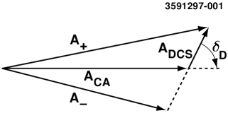
FIG. 8.: Obtaining the phase $\Delta_{D}$ of Equation (C1) from the Cabibbo allowed $D^{0}$ decay amplitude, $A_{CA}$, the doubly Cabibbo suppressed amplitude, $A_{DCS}$, and their interference, $A_{\pm}\equiv A_{CA}\pm A_{DCS}$.

We proceed to study the measurement of $\Delta_{D}$ at a charm factory, operating at the $\psi(3770)$ resonance. For simplicity, we will discuss this measurement in the context of the SM. Given the current bounds on $x_{D}$ and $y_{D}$, we expect this measurement to be rather insensitive to $D^{0}-\overline{D^{0}}$ mixing. The relation

$$\Delta_{D}={\rm arg}\left[A(D^{0}\rightarrow f_{D})A(\overline{D^{0}}\rightarrow f_{D})^{*}\right]$$ (C1)

is graphically represented in Figure 8, demonstrating how to obtain $\Delta_{D}$ from the the Cabibbo allowed $D$ decay amplitude, $A_{CA}$, the doubly Cabibbo suppressed amplitude, $A_{DCS}$, and their interference, $A_{\pm}\equiv A_{CA}\pm A_{DCS}$. While $A_{CA}$ and $A_{DCS}$ have been measured at CLEO [17] for the $K^{-}\pi^{+}$ mode by using $D^{*+}$ decays to tag the $D^{0}$ flavor, measuring $A_{\pm}$ requires producing $D^{0}-\overline{D^{0}}$ pairs in a known coherent state. It is therefore best to perform all three measurements at the charm factory, canceling many systematic errors in the construction of the triangles of Figure 8. To measure the amplitude $A_{+}$ ($A_{-}$), one of the $\psi(3770)$ daughters is tagged as a $D^{0}_{-}$ ($D^{0}_{+}$) by observing it decay into a CP-odd (CP-even) state, such as $K_{S}\;\pi^{0}$ ($K^{+}K^{-}$). The other daughter is then $D^{0}_{+}$ ($D^{0}_{-}$), and the fraction of the time that it is seen decaying into $K^{-}\pi^{+}$ gives the interference amplitude ${1\over 2}|A_{\pm}|^{2}$. We immediately find

$$\cos\Delta_{D}=\pm{|A_{\pm}|^{2}-|A_{CA}|^{2}-|A_{DCS}|^{2}\over 2|A_{CA}||A_{DCS}|}.$$ (C2)

Due to the low statistics tagging scheme of the $|A_{\pm}|$ measurement and the fact that $\left|A_{DCS}\right|\ll\left|A_{CA}\right|$, the error in $\cos\Delta_{D}$ is dominated by the $|A_{\pm}|$ measurement error. Hence

$$\sigma_{\cos\Delta_{D}} \approx {\sigma_{|A_{\pm}|}\over\left|A_{DCS}\right|}\approx{\sigma_{|A_{\pm}|}\over|A_{\pm}|}\;\left|{A_{CA}\over A_{DCS}}\right|$$ (C3)

$$= {1\over 2\sqrt{N_{A_{\pm}}}}\;\left|A_{CA}\over A_{DCS}\right|,$$ (C4)

where $N_{A_{\pm}}$ is the number of events observed in the $A_{\pm}$ channels, and we made use of $\left|A_{CA}\right|\approx\left|A_{\pm}\right|$. Since the event is fully reconstructed, background is expected to be small, and its contribution to $\sigma_{\cos\Delta_{D}}$ is neglected in this discussion. $N_{A_{\pm}}$ is given by

$$N_{A_{\pm}} = N_{D\overline{D}}\ {\cal B}(D^{0}\rightarrow K^{-}\pi^{+})\;\epsilon(K^{-}\pi^{+})$$ (C5)

$$\times \sum_{i}{\cal B}(D^{0}\rightarrow t_{i})\;\epsilon(t_{i}),$$ (C6)

where $N_{D\overline{D}}$ is the number of $\psi(3770)\rightarrow D^{0}\overline{D}^{0}$ events, $t_{i}$ are the CP-eigenstates used for tagging, and $\epsilon(X)$ is the reconstruction efficiency of the state $X$. Taking [6] $\sum_{i}{\cal B}(D^{0}\rightarrow t_{i})\;\epsilon(t_{i})\approx 0.02$, $\epsilon(K^{-}\pi^{+})\approx 0.8$ and $\left|A_{CA}/A_{DCS}\right|=1/\sqrt{0.0031}$, and ${\cal B}(D^{0}\rightarrow K^{-}\pi^{+})\approx 0.04$, Eq. (C4) becomes

$$\sigma_{\cos\Delta_{D}}\approx{370\over\sqrt{N_{D\overline{D}}}}.$$ (C7)

It is expected that in one year the charm factory will collect 10 $\rm fb^{-1}$, or $N_{D\overline{D}}=2.9\times 10^{7}$ [25], resulting in $\sigma_{\cos\Delta_{D}}\approx 0.065$. Thus, $\cos\Delta_{D}$ can be measured to high precision, even in the presence of background and with relatively modest luminosity. We note that the same measurement technique can be used with multi-body $D^{0}$ decays, in which $\cos\Delta_{D}$ varies over the available phase space. While the relative statistical error in every small region of phase space will be large, its effect on the measurement of $\gamma$ in $B\rightarrow DK$ will be proportionally small. The total error in $\gamma$ due to $\Delta\cos\Delta_{D}$ will be as small as in the two body $K^{-}\pi^{+}$ mode, up to differences in $D^{0}$ branching fractions, reconstruction efficiencies, and backgrounds.

REFERENCES

- [1] N. Cabibbo, Phys. Rev. Lett. 10, 531 (1963); M. Kobayashi and T. Maskawa, Prog. Theor. Phys. 49, 652 (1973).
- [2] CLEO Collaboration, B. Barish et al., Report No. CLEO CONF 97-01, EPS 339.
- [3] M. Gronau and D. London, Phys. Lett. B 253, 483 (1991).
- [4] M. Gronau and D. Wyler, Phys. Lett. B 265, 172 (1991).
- [5] D. Atwood, I. Dunietz, and A. Soni, Phys. Rev. Lett. 78, 3257 (1997).
- [6] A. Soffer, Phys. Rev. D 60, 054032 (1999).
- [7] C. C. Meca and J. P. Silva, Phys. Rev. Lett. 81, 1377 (1998). See also Ref. [8]
- [8] A. Amorim, M. G. Santos, and J. P. Silva, Phys. Rev. D 59, 056001 (1999).
- [9] R. Aleksan, B. Kayser, and D. London, Phys. Rev. Lett. 73, 18 (1994).
- [10] See, for example, G. C. Branco, L. Lavoura, and J. P. Silva, CP Violation (Oxford University Press, Oxford, 1999), and references therein.
- [11] S. Bergmann and Y. Nir, J. High Energy Phys. 9909, 031 (1999).
- [12] A. Ali and D. London, Eur. Phys. J. C 9, 687 (1999).
- [13] A. J. Buras, Lectures given at the 14th Lake Louise Winter Institute (1999), hep-ex/9905437.
- [14] CLEO Collaboration, J. P. Alexander et al., Phys. Rev. Lett. 77, 5000 (1996).
- [15] C. Caso et al., European Physical Journal C3, 1 (1998), and also the URL: http://pdg.lbl.gov.
- [16] CLEO Collaboration, M. Athanas et al., Phys. Rev. Lett. 80, 5493 (1998).
- [17] J. Gronberg, ‘ mixing at CLEO-II’, to appear in Proc. 1999 Division of Particles and Fields Conference, Los Angeles, CA, U.S.A., Jan. 5-9, 1999. In [5] the then-current value of 0.0077 was used for Eq. (14).
- [18] H. N. Nelson, hep-ex/9909028, talk presented at 1999 Chicago Conference on Kaon Physics (K 99), Chicago, (1999). The bounds obtained in this reference refer to new quantities and , where is the strong phase difference in the decays used in the study. They find and at the C. L. The bound we quote in Eq. (15) results from the fact that .
- [19] H. N. Nelson, private communication.
- [20] For a review see, for example, H. N. Nelson, hep-ex/9908021.
- [21] F. Bucella, M. Lusignoli, and A. Pugliese, Phys. Lett. B 379, 249 (1996).
- [22] For example, the prediction for Babar can be found in The BaBar physics book, edited by P. F. Harrison and H. R. Quinn (SLAC, Stanford, 1998), page 798. There a sensitivity estimate for of is quoted for a year running at nominal luminosity.
- [23] H. Yamamoto , CBX 94-14, HUTP-94/A006; H. N. Nelson, private communication.
- [24] T. Liu, Harvard University preprint number HUTP-94/E021, in Proceedings of the Charm 2000 Workshop, FERMILAB-Conf-94/190, page 375, 1994. L. Wolfenstein, Phys. Rev. Lett. 75, 2460 (1995). G. Blaylock, A. Seiden, and Y. Nir, Phys. Lett. B 355, 555 (1995). T. E. Browder and S. Pakvasa, Phys. Lett. B 383, 475 (1996). See also Ref. [18].
- [25] J. Kirkby, in La Thuile 1996, Results and Perspectives in Particle Physics, 747 (1996).