CFNUL/99-10
hep-ph/9912240

Neutrino mixing scenarios and AGN

Abstract

Active galactic nuclei (AGN) have been suggested to be sources of very high energy neutrinos. We consider the possibility of using AGN neutrinos to test neutrino mixings. From the atmospheric, solar and laboratory data on neutrino oscillations we derive the flavour composition of the AGN neutrino flux in different neutrino mixing schemes. We show that most of the schemes considered can be distinguished from each other and the existence of a sterile neutrino can be specially tested. AGN neutrinos can also be used to test those four-neutrino scenarios where solar neutrinos oscillate into an arbitrary mixture of $\nu_{s}$ and $\nu_{\tau}$.

PACS: 14.60.Lm; 14.60.Pq; 14.60.St; 98.54.Cm

Keywords: active galactic nuclei; neutrino mixing

¹lbento@fc.ul.pt ²keranen@alf1.cii.fc.ul.pt ³jukka.maalampi@helsinki.fi

Introduction. Atmospheric and solar neutrino measurements have provided a strong evidence for the existence of neutrino oscillations, or neutrino masses and mixings. The recent atmospheric neutrino results from Super-Kamiokande [1] suggest the oscillation of the muon neutrino ($\nu_{\mu}$) into a tau neutrino ($\nu_{\tau}$) or a sterile neutrino ($\nu_{s}$). On the other hand, the observed solar neutrino deficit can be interpreted as evidence for the oscillation of the electron neutrinos ($\nu_{e}$) into neutrinos of a different flavour (see e.g. [2, 3]). In addition, the LSND collaboration has reported results of their laboratory measurements that indicate the existence of $\bar{\nu}_{\mu}\rightarrow\bar{\nu}_{e}$ and $\nu_{\mu}\rightarrow\nu_{e}$ oscillations [4]. Unfortunately, the data does not yet uniquely fix the mass and mixing pattern among neutrinos. A number of different scenarios are still allowed.

The explanation of the solar, atmospheric and LSND results requires a four-neutrino scheme of three active neutrinos $\nu_{e}$, $\nu_{\mu}$, $\nu_{\tau}$ and one sterile neutrino $\nu_{s}$ [5]. The mass pattern should have a two-doublet structure [6]: one of the doublets consists of $\nu_{e}$ and $\nu_{s}$ (or $\nu_{e}$ and $\nu_{\tau}$), and is responsible for the solar neutrino deficit, and the other one, responsible for the atmospheric neutrino anomaly, consists of $\nu_{\mu}$ and $\nu_{\tau}$ (or $\nu_{\mu}$ and $\nu_{s}$). These doublets are separated by a wide mass gap (${\cal O}(1{\rm\ eV})$), so as to explain the LSND result in terms of $\nu_{e}-\nu_{\mu}$ mixing.

There is an ambiguity in this scheme due to the fact that there are at present four viable interpretations of the solar neutrino data corresponding to different choices of the oscillation parameters: the vacuum oscillation solution (VO), the low MSW solution (LOW), the small mixing angle MSW solution (SMA) and the large mixing angle MSW solution (LMA) [2, 3]. Disregarding the LSND data, it is, of course, possible to give an explanation for the other results in terms of the known three neutrino species. In this case one assumes that the atmospheric neutrino anomaly is due to $\nu_{\mu}-\nu_{\tau}$ mixing and solar neutrinos oscillate to $\nu_{\mu}$ and $\nu_{\tau}$. On the other hand, there might exist two (or more) sterile neutrinos ($\nu_{s}$, $\nu_{s^{\prime}}$) so that the solar neutrino deficit is due to $\nu_{e}-\nu_{s}$ mixing and the atmospheric neutrino anomaly due to $\nu_{\mu}-\nu_{s^{\prime}}$ mixing.

In this paper we will study the possibility of testing the various neutrino mixing scenarios by observing the flavour composition of the high-energy neutrino flux from active galactic nuclei (AGN). With the oscillation parameters suggested by the solar neutrino, the atmospheric neutrino and the laboratory measurements, the fluxes of different neutrino flavours are determined entirely by the mixing angles with no dependence on the masses. It turns out that there are quite large variations of the fluxes between the different mixing schemes, which should be detectable in the new neutrino telescopes [7] such as AMANDA, NESTOR, BAIKAL, ANTARES and NEMO. With sufficient statistics, which we believe to be achievable in these telescopes within a reasonable time scale, one would be able to discriminate between different solar neutrino solutions, check the possible existence of large active-sterile mixings, and make distinction between three-neutrino and most of the four-neutrino schemes.

Production of AGN neutrinos. The AGN neutrino production is suggested to take place in the AGN cores [8], in the jets [9] and at the endpoints of jets so-called hot spots [10]. In these sources, charged particles are supposed to be accelerated in the vicinity of shock waves by the first order Fermi acceleration mechanism (see e.g. [11]). The collisions of the accelerated protons with photons in the ambient electromagnetic fields would then lead to the production of energetic gamma rays and neutrinos via the pion photoproduction processes [12],

$$\mbox{$$}p\gamma \rightarrow n\pi^{+}\rightarrow\mu^{+}\nu_{\mu}\rightarrow e^{+}\nu_{e}\bar{\nu}_{\mu},$$

$$p\gamma \rightarrow p\pi^{0}\rightarrow 2\gamma.\vspace{\undereqskip}$$ (1)

The neutrino and high energy photon spectra are thus related to each other, and the neutrino flux can be estimated from the high energy photon flux [12, 13]. Tau neutrinos are produced in negligible amounts [14]. Hence the flavour composition of the AGN neutrino flux is expected to be, with a high precision,

$$N_{\tau}:N_{\mu}:N_{e}=0:2:1,$$ (2)

where $N_{\alpha}$, $\alpha=e,\mu,\tau$, denotes the total flux of $\nu_{\alpha}$’s and $\bar{\nu}_{\alpha}$’s.

The integrated diffuse intensity of high-energy ($E_{\nu}>10{\rm\ TeV}$) neutrinos from AGN and blazars detected in a detector with an effective area of $1\ {\rm km}^{2}$ has been estimated to be a few hundreds per year [13]. When the plans to build several km-scale detectors become reality, the total annual flux observed will be, if these estimates turn out to be correct, of the order of some hundreds to one thousand neutrinos. This is much larger than the estimated background flux of atmospheric neutrinos in the same energy range. On the other hand, the flavour composition of the atmospheric neutrino flux will be quite well understood due to the measurements at the lower part of the energy spectrum. Hence the background of the atmospheric neutrinos would not crucially interfere with the determination of the AGN neutrino fluxes. Therefore the detection of AGN neutrinos will probe new physics beyond the Standard Model (SM), in particular neutrino oscillations [14].

It is important to notice that all three neutrino flavours will be observed independently from each other [12, 14, 15]. Therefore any new physics beyond the SM that may alter the flavour composition of the neutrino flux will be probed. Neutrino oscillations can be tested by using the flavour composition [14], but AGN neutrino flux is sensitive also to other phenomena, such as new interactions, magnetic moments and decays of neutrinos, which may affect the intensity or the composition of the flux [16]. Here we shall study how the AGN neutrino data might be used to discriminate between various neutrino mixing schemes proposed for the interpretation of the results of the solar, atmospheric and LSND neutrino experiments.

Oscillation probabilities. In the four-neutrino scenarios mentioned above, the neutrinos form two pairs of flavours with a large or potentially large mixing within each pair. In the two basic scenarios that can be considered [6] all the other mixing angles are small and they cannot substantially affect the flavour composition of the AGN neutrino flux. In that case it is sufficient to consider two-flavour oscillations with either atmospheric or solar neutrino mixing angles $\theta_{\rm atm}$ and $\theta_{\odot}$, respectively.

The oscillation probability for the two-neutrino oscillation $\nu_{\alpha}\rightarrow\nu_{\beta}$ ($\alpha\not=\beta$) is given by

$$P(\nu_{\alpha}\to\nu_{\beta})=\frac{1}{2}\sin^{2}2\theta_{\alpha\beta}\left(1-\cos\left(\frac{\Delta m^{2}L}{2E}\right)\right),$$ (3)

where $\Delta m^{2}$ is the squared mass difference of the corresponding mass eigenstates and $\theta_{\alpha\beta}$ is the mixing angle. Due to the enormous distance $L$ to the source (typically $L\simeq 500$ Mpc) the AGN neutrino oscillations can be relevant to probe squared mass differences of the order $10^{-16}{\rm\ eV}^{2}$ for the typical AGN neutrino energies of the order of PeV. Turning this argument around, one can say that for any value of $\Delta m^{2}$ implied by the present experimental results the oscillating term averages to zero when integrated over the neutrino energy spectrum. Obviously, matter effects could only be relevant for the neutrinos that pass across the Earth. But, in this case, for such high energies, the weak eigenstates form effective mass eigenstates and decouple from each others. The transition probabilities $P(\nu_{\alpha}\rightarrow\nu_{\beta})$ and $P(\nu_{\alpha}\rightarrow\nu_{\alpha})$ are thus entirely determined by the mixing angles $\theta_{\alpha\beta}$ between the flavour states $\nu_{\alpha}$ and $\nu_{\beta}$:

$$\mbox{$$}P(\nu_{\alpha}\to\nu_{\beta})=\frac{1}{2}\sin^{2}2\theta_{\alpha\beta},\ P(\nu_{\alpha}\to\nu_{\alpha})=1-\frac{1}{2}\sin^{2}2\theta_{\alpha\beta}\;.\vspace{\undereqskip}$$ (4)

Four-neutrino models. Let us first consider the four-neutrino scheme where $\nu_{\mu}$ mixes maximally or almost maximally ($0.8\;\raise 1.29167pt\hbox{$<$\kern-7.5pt\raise-4.73611pt\hbox{$\sim$}}\;\sin^{2}2\theta_{\mathrm{atm}}\leq 1.0$) with $\nu_{\tau}$ to account for the atmospheric neutrino anomaly while the oscillations of $\nu_{e}$ into sterile neutrinos $\nu_{s}$ explain the solar neutrino deficit. Let $N_{e}=1$, $N_{\mu}=2$, $N_{\tau}=0$ be the normalized neutrino fluxes with the relative rates as predicted by the SM, that is, if there are no neutrino mixings. Then, the predicted rates for $\nu_{e}$, $\nu_{\mu}$, $\nu_{\tau}$ and $\nu_{s}$ in this four-neutrino scenario are

$$N_{e} =1-\frac{1}{2}\sin^{2}2\theta_{\odot}\;,$$

$$N_{\mu} =2-\sin^{2}2\theta_{\mathrm{atm}}\;,$$

$$N_{\tau} =\sin^{2}2\theta_{\mathrm{atm}}\;,$$

$$N_{s} =\frac{1}{2}\sin^{2}2\theta_{\odot}\;.$$ (5)

According to recent studies only a small MSW mixing angle $\theta_{\odot}$ can fit the solar neutrino data with a sterile neutrino option [2, 3]. Thus the $\nu_{e}-\nu_{s}$ mixing will not substantially affect the composition of the AGN neutrino flux, and one predicts the following observable ratios of neutrino fluxes:

$$\frac{2N_{e}}{N_{\mu}+N_{\tau}} =1\;,$$

$$\frac{2N_{\tau}}{N_{\mu}+N_{\tau}} =\sin^{2}2\theta_{\mathrm{atm}}\;.$$ (6)

The latter ratio would provide a new independent measurement for the atmospheric neutrino mixing angle $\theta_{\mathrm{atm}}$.

In the other four-neutrino scenario, the atmospheric neutrino anomaly is explained in terms of $\nu_{\mu}-\nu_{s}$ oscillations and the solar neutrino deficit in terms of $\nu_{e}-\nu_{\tau}$ oscillations. In the solar case various types of solutions can fit the data, three of them with a large mixing angle [2, 3]: the vacuum oscillation solution (VO) with $0.7\;\raise 1.29167pt\hbox{$<$\kern-7.5pt\raise-4.73611pt\hbox{$\sim$}}\;\sin^{2}2\theta_{\odot}\;\raise 1.29167pt\hbox{$<$\kern-7.5pt\raise-4.73611pt\hbox{$\sim$}}\;1.0$, the LOW solution with $0.9\;\raise 1.29167pt\hbox{$<$\kern-7.5pt\raise-4.73611pt\hbox{$\sim$}}\;\sin^{2}2\theta_{\odot}\;\raise 1.29167pt\hbox{$<$\kern-7.5pt\raise-4.73611pt\hbox{$\sim$}}\;1.0$ and the large mixing angle (LMA) MSW solution with $0.55\;\raise 1.29167pt\hbox{$<$\kern-7.5pt\raise-4.73611pt\hbox{$\sim$}}\;\sin^{2}2\theta\;\raise 1.29167pt\hbox{$<$\kern-7.5pt\raise-4.73611pt\hbox{$\sim$}}\;0.96$. The latter is now preferred as a result of the Super-Kamiokande energy spectrum data [17]. In all these three cases, $\sin^{2}2\theta_{\odot}$ lies above 1/2, and this is the constraint we will use below. In the small mixing angle (SMA) MSW solution $\sin^{2}2\theta_{\odot}$ is very small and can be neglected. The $\nu_{e}$ and the $\nu_{\mu}$ rates are the same as in the previous scenario, given in (5), but the $\nu_{\tau}$ and the $\nu_{s}$ rates are interchanged, i.e.

$$N_{\tau} =\frac{1}{2}\sin^{2}2\theta_{\odot}\;,$$

$$N_{s} =\sin^{2}2\theta_{\mathrm{atm}}\;.$$ (7)

One interesting observable flux ratio is

$$\mbox{$$}\frac{2N_{\tau}}{N_{e}+N_{\tau}}=\sin^{2}2\theta_{\odot}\;,\vspace{\undereqskip}$$ (8)

which provides an independent measurement of the solar neutrino mixing angle $\theta_{\odot}$. Naturally this ratio distinguishes between the large solar mixing angle solutions, i.e. VO, LMA and LOW, and the SMA solution: there is no $\nu_{\tau}$ component in the flux in the latter case. Another useful observable is the ratio of the $\nu_{\mu}$ flux to the $\nu_{e}$ and $\nu_{\tau}$ fluxes, for which one has the bounds

$$\mbox{$$}1\leqslant\frac{N_{\mu}}{N_{e}+N_{\tau}}=2-\sin^{2}2\theta_{\mathrm{atm}}\lesssim 1.2\;,\vspace{\undereqskip}$$ (9)

where the upper limit comes from the constraint $\sin^{2}2\theta_{\mathrm{atm}}\gtrsim 0.8$. (Note that if neutrinos did not mix this ratio had the value 2.)

The ratio (9) can be used to make a distinction between the scheme where the solar neutrino deficit is explained with the $\nu_{e}-\nu_{\tau}$ oscillations and the scheme where it is done with a $\nu_{e}-\nu_{s}$ mixings. In the latter case (see Eqs. (5)) the ratio is bounded as

$$\frac{1}{2}\leqslant\frac{N_{\mu}}{N_{e}+N_{\tau}}\lesssim\frac{2}{3}\;.$$ (10)

The contrast between the two four-neutrino scenarios is evident. Let us note that if the solar neutrino deficit is due to large $\nu_{e}-\nu_{s}$ mixing ($\sin^{2}2\theta_{\odot}\;\raise 1.29167pt\hbox{$>$\kern-7.5pt\raise-4.73611pt\hbox{$\sim$}}\;\frac{1}{2}$), the ratio (9) varies between 0.7 and 0.9. This solution is, however, strongly disfavoured by the present data [2, 3].

The predictions of the different neutrino mixing scenarios can be described in terms of the relative ’abundances’ of neutrino flavours defined as

$$y_{\alpha}=\frac{3N_{\alpha}}{N_{e}+N_{\mu}+N_{\tau}}\;,\qquad\qquad\alpha=e,\mu,\tau\;,$$ (11)

which obey the relation $y_{e}+y_{\mu}+y_{\tau}=3$. In the case of no mixing (SM) one has $y_{e}=1$, $y_{\mu}=2$ and $y_{\tau}=0$. In Fig. 1 we present the allowed regions in the $y_{\mu}-y_{\tau}$ plane for each of the scenarios. The two straight solid lines correspond to SMA MSW solutions of the solar neutrino deficit and the two quadrangular areas with dashed lines to all of the solutions with a large mixing angle, $0.5\;\raise 1.29167pt\hbox{$<$\kern-7.5pt\raise-4.73611pt\hbox{$\sim$}}\;\sin^{2}2\theta_{\odot}\leq 1$ (LMA, LOW and VO). The straight line labeled with $\nu_{s}$ corresponds to the four-neutrino scheme where $\nu_{e}-\nu_{s}$ mixing solves the solar neutrino deficit, and the other line (labeled with $\nu_{\tau}$), lying on the $y_{\mu}$-axis, corresponds to the scenario where it is explained in terms of $\nu_{e}-\nu_{\tau}$ mixing. The lower quadrangular area labeled with $\nu_{\tau}$ corresponds to the scenario where $\nu_{e}-\nu_{\tau}$ mixing solves the solar neutrino deficit and the area labeled with $\nu_{s}$ to the scheme where it is solved by $\nu_{e}-\nu_{s}$ mixing and the atmospheric neutrino anomaly by $\nu_{\mu}-\nu_{\tau}$ oscillations. As mentioned above, the latter is disfavoured by the solar neutrino data [2, 3]. Along each of the solid or dashed lines either $\theta_{\odot}$ or $\theta_{\rm atm}$ is constant. As $\sin^{2}2\theta_{\rm atm}$ increases from 0.8 to 1 the abundance $y_{\mu}$ always decreases, and the growth of $\sin^{2}2\theta_{\odot}$ from 0.5 to 1 is indicated by arrows. Hence the maximal mixing point $\sin^{2}2\theta_{\odot}=\sin^{2}2\theta_{\rm atm}=1$ is the upper left corner in the lower ”quadrangle” and the upper right corner in the other one.

The basic scenarios studied so far may be considered as extreme cases of a more general four-neutrino scenario where solar electron neutrinos oscillate not to a pure sterile $\nu_{s}$ or a pure active $\nu_{\tau}$ neutrino flavour but rather to some linear combination $\nu_{x}\equiv\cos\theta\;\nu_{s}-\sin\theta\;\nu_{\tau}$ of those two. The atmospheric muon neutrinos would then oscillate into the corresponding orthogonal superposition $\nu_{y}\equiv\sin\theta\;\nu_{s}+\cos\theta\;\nu_{\tau}$. This kind of situation is perfectly consistent with the limits [6] derived from the reactor disappearance experiments and with the atmospheric neutrino observations as well. As to solar neutrinos, so far there does not exist a data analysis for this $\nu_{e}-\nu_{s}-\nu_{\tau}$ three-neutrino mixing scheme, as complete as what has been done for the $\nu_{e}-\nu_{s}$ or $\nu_{e}-\nu_{\tau}$ two-neutrino oscillation schemes [2, 3, 17]. Let $\nu_{1}$, $\nu_{2}$ be the mass eigenstates responsible for the solar neutrino deficit and $\nu_{3}$, $\nu_{4}$ the states involved in atmospheric neutrino oscillations. The two pairs are separated by the LSND mass gap but no other specific mass hierarchy has to be assumed. The reactor experiments constrain the mixing matrix elements $U_{e3}$, $U_{e4}$, $U_{\mu 1}$, $U_{\mu 2}$ to be small [6] but not $U_{\tau i}$ or $U_{si}$. If one drops all the mixing angles that are necessarily small (unimportant for our purpose), the mixing matrix is given as follows:

$$\nu_{1} =\cos\theta_{\odot}\;\nu_{e}-\sin\theta_{\odot}(\cos\theta\;\nu_{s}-\sin\theta\;\nu_{\tau})\;,$$

$$\nu_{2} =\sin\theta_{\odot}\;\nu_{e}\;+\cos\theta_{\odot}(\cos\theta\;\nu_{s}-\sin\theta\;\nu_{\tau})\;,$$

$$\nu_{3} =\cos\theta_{\mathrm{atm}}\;\nu_{\mu}-\sin\theta_{\mathrm{atm}}(\sin\theta\;\nu_{s}+\cos\theta\;\nu_{\tau})\;,$$

$$\nu_{4} =\sin\theta_{\mathrm{atm}}\;\nu_{\mu}+\cos\theta_{\mathrm{atm}}(\sin\theta\;\nu_{s}+\cos\theta\;\nu_{\tau})\;.$$ (12)

It is clear that the solar and atmospheric neutrino phenomena are understood in terms of $\nu_{e}-\nu_{x}$ and $\nu_{\mu}-\nu_{y}$ oscillations, respectively ($\nu_{x}$ and $\nu_{y}$ are the states inside brackets).

The predicted rates of AGN neutrinos are now

$$N_{\tau} =\cos^{2}\theta\,\sin^{2}2\theta_{\mathrm{atm}}+\frac{1}{2}\sin^{2}\theta\,\sin^{2}2\theta_{\odot}\;,$$

$$N_{s} =\sin^{2}\theta\,\sin^{2}2\theta_{\mathrm{atm}}+\frac{1}{2}\cos^{2}\theta\,\sin^{2}2\theta_{\odot}\;,$$ (13)

while the rates of $\nu_{e}$ and $\nu_{\mu}$ remain the same as in Eqs. (5). If the angle $\theta$ is set to be an arbitrary parameter the allowed regions are enlarged covering the two more specific schemes considered before. There are two different regions, both limited by dotted lines: one is for solar SMA solutions and the other for large solar mixing angle solutions LMA, LOW and VO. The angle $\theta$ varies along the dotted lines: one has $\theta=0$ for the $\nu_{e}-\nu_{s}$ solar neutrino mixing scheme and $\theta=\pi/2$ for the $\nu_{e}-\nu_{\tau}$ mixing scheme. If the AGN neutrino data turns out to lie outside the areas for these two specific schemes it will indicate that solar neutrinos do not oscillate to pure active or sterile neutrino states but rather to a mixture of them.

Three-neutrino model. A radically different scenario is the one with just the three standard model neutrinos. That is enough for explaining the atmospheric and solar neutrino data when the LSND results are disregarded. It is worthwhile to check if the AGN high-energy neutrinos can be used to confirm or disprove such a three-neutrino hypothesis. In the viable three-neutrino scenario the atmospheric $\nu_{\mu}$’s essentially oscillate to $\nu_{\tau}$ but not to $\nu_{e}$, as indicated by the Super-Kamiokande [1] and Chooz data [18]. If $\nu_{\mu}$ and $\nu_{\tau}$  are maximally mixed the prediction for the AGN neutrinos is that half of the $\nu_{\mu}$’s are converted into $\nu_{\tau}$’s making all the observable fluxes of the flavours $\nu_{e}$, $\nu_{\mu}$ and $\nu_{\tau}$ equal to each other, irrespectively to the value of the solar neutrino mixing angle $\theta_{\odot}$. The situation changes, however, if the atmospheric neutrino mixing is not maximal.

In the three-neutrino scheme the solar electron neutrinos oscillate into a particular superposition of $\nu_{\mu}$ and $\nu_{\tau}$ with which $\nu_{e}$ forms a pair of almost degenerate mass eigenstates, $\nu_{1}$ and $\nu_{2}$, separated from the mass eigenstate $\nu_{3}$ by the mass gap $\Delta m_{\mathrm{atm}}^{2}\simeq(2-6)\times 10^{-3}{\rm\ eV}^{2}$. The limits obtained by the Super-Kamiokande [1] and Chooz [18] experiments imply that $\nu_{e}$ is only a small fraction of the mass eigenstate $\nu_{3}$, that is, the element $U_{e3}$ of the rotation matrix is small. For our purpose this mixing can be neglected and will be taken to be zero. Then the matrix elements $U_{\alpha i}$ can be read from

$$\mbox{$$}\nu_{e} = \cos\theta_{\odot}\;\nu_{1}+\sin\theta_{\odot}\;\nu_{2}\;,$$

$$\nu_{\mu} = \cos\theta_{\mathrm{atm}}(-\sin\theta_{\odot}\;\nu_{1}+\cos\theta_{\odot}\;\nu_{2})+\sin\theta_{\mathrm{atm}}\;\nu_{3}\;,$$

$$\nu_{\tau} = -\sin\theta_{\mathrm{atm}}(-\sin\theta_{\odot}\;\nu_{1}+\cos\theta_{\odot}\;\nu_{2})+\cos\theta_{\mathrm{atm}}\;\nu_{3}\;.\vspace{\undereqskip}$$ (14)

The mass eigenstates $\nu_{1}$ and $\nu_{2}$ are of course separated by the gap $\Delta m_{\odot}^{2}$.

After many oscillation lengths the number of neutrinos with a given flavour, $N_{\alpha}$, averages to an amount that is related to the rates of originally emitted neutrinos, $N_{\beta}^{0}$, as follows:

$$N_{\alpha}=\sum_{i,\beta}\left|U_{\alpha i}U_{i\beta}^{\dagger}\right|^{2}N_{\beta}^{0}\;.$$ (15)

Using the same normalization as before, i.e. $N_{e}^{0}=1$, $N_{\mu}^{0}=2$, $N_{\tau}^{0}=0$, one obtains

$$\mbox{$$}N_{e} = 1+\frac{1}{2}\sin^{2}2\theta_{\odot}\cos 2\theta_{\rm{atm}}\;,$$

$$N_{\mu} = 2-\sin^{2}2\theta_{\rm{atm}}-\frac{1}{2}\sin^{2}2\theta_{\odot}\cos 2\theta_{\rm{atm}}\cos^{2}\theta_{\rm{atm}}\;,$$

$$N_{\tau} = \sin^{2}2\theta_{\rm{atm}}-\frac{1}{2}\sin^{2}2\theta_{\odot}\cos 2\theta_{\rm{atm}}\sin^{2}\theta_{\rm{atm}}\;.\vspace{\undereqskip}$$ (16)

The total number of neutrinos is conserved and equal to 3 in this normalization. If $\theta_{\mathrm{atm}}$ is maximal one gets equally distributed fluxes over all flavours, as expected. If $\theta_{\mathrm{atm}}$ is not maximal the relative rates change and, interestingly enough, are sensitive to the sign of $\cos 2\theta_{\mathrm{atm}}$, thus differentiating between a mixing angle $\theta_{\mathrm{atm}}$ larger than $\pi/4$ from a mixing angle smaller than $\pi/4$. This can be seen in Fig. 1, where the two small triangular-like areas correspond to $\sin^{2}2\theta_{\mathrm{atm}}$ between $0.8$ and $1$ and $\sin^{2}2\theta_{\odot}$ from $1/2$ to $1$. The upper ”triangle” corresponds to a negative $\cos 2\theta_{\mathrm{atm}}$ and the lower ”triangle” to a positive $\cos 2\theta_{\mathrm{atm}}$, and they meet at the point of maximal mixing, $\theta_{\mathrm{atm}}=\pi/4$. Hence, the AGN neutrinos may be used, in principle at least, to discriminate between a negative and a positive $\cos 2\theta_{\mathrm{atm}}$. The sensitivity is best when $\sin^{2}2\theta_{\rm atm}=0.8$ and $\sin^{2}2\theta_{\odot}=1$, corresponding to the most distant points of the two ”triangles”. The small $\theta_{\odot}$ solution (SMA) identifies with the straight line starting at the $(1,1)$ point, the same as for the four-neutrino scheme with solar SMA $\nu_{e}-\nu_{s}$ mixing. Apart from that, the three-neutrino scenario is in general quite distinct from the four-neutrino schemes.

Exotic scenarios. One can find in the literature still some other oscillation scenarios in addition to the three-neutrino and four-neutrino models considered above, which may lead to different predictions for the flux composition. Models have been proposed  [19] with more than one sterile neutrino where the solar neutrino deficit is explained in terms of $\nu_{e}-\nu_{s}$ mixing and the atmospheric neutrino anomaly in terms of $\nu_{\mu}-\nu_{s^{\prime}}$ mixing, where $\nu_{s}$ and $\nu_{s^{\prime}}$ are two separate sterile states. The prediction is in that case, within the SMA solar neutrino solution, $1.5\;\raise 1.29167pt\hbox{$<$\kern-7.5pt\raise-4.73611pt\hbox{$\sim$}}\;y_{\mu}\;\raise 1.29167pt\hbox{$<$\kern-7.5pt\raise-4.73611pt\hbox{$\sim$}}\;1.6$ and $y_{\tau}=0$, the same as in the four-neutrino scheme with solar $\nu_{e}-\nu_{\tau}$ SMA solution. These two cases cannot be distinguished with AGN neutrino data only. Of course, there could also exist a sterile neutrino very degenarate with one of the active neutrinos, so that the squared mass difference is below the values probed in other phenomena. Such a neutrino could have visible effects on the AGN neutrino flux if its mixing with one of the active neutrinos is large.

Cosmic connection. Let us finally note that the question of existence of sterile neutrinos and their mixings with active neutrinos has relevance also for cosmology. Depending on the value of $\Delta m^{2}$, a large active-sterile neutrino mixing could bring sterile neutrinos into thermal equilibrium thereby increasing the effective number of light neutrinos, $N_{\nu}$ [20]. According to a recent analysis [21] the abundancies of light elements yield the upper bound $N_{\nu}\leq 3.20$, which sets very tight constraints on the active-sterile mixings, in particular on the $\nu_{\mu}-\nu_{s}$ mixing [22]. The four-neutrino scenario where the atmospheric neutrino anomaly is explained in terms of the $\nu_{\mu}-\nu_{s}$ mixing seems hence unprobable. A large $\nu_{e}-\nu_{s}$ mixing is less stringently constained by this argument as the value of $\Delta m^{2}$ for the solar neutrinos is smaller than for the atmospheric neutrinos. The cosmological bound on $N_{\nu}$ is a disputable matter. Some observations have indicated a higher primordial deuterium abundancy than normally assumed, and this leads to a less restrictive limit on the effective number of light neutrinos [23]. The conflict with the nucleosynthesis bounds may also be avoided with a large lepton asymmetry [24]. The AGN flux measurements would provide a new way to check the consistency of this cosmological reasoning.

Conclusions. In conclusion, if neutrinos turn out to be produced in AGN with the rates as suggested by some authors [8, 9, 10], then the measurement of the flavour composition of the AGN neutrino flux will provide a new method to discriminate between various neutrino oscillation schemes for solar, atmospheric and laboratory neutrinos. It would also offer a new independent measurement of the various mixing angles, such as the atmospheric and solar neutrino mixing angle $\theta_{\rm atm}$ and $\theta_{\odot}$. Of particular interest is the possibility of testing the existence of sterile neutrinos and of making a distinction between small and large angle active-sterile mixing. Moreover, one may have a hint of the more general four-neutrino scenarios with large $\nu_{\tau}-\nu_{s}$ mixing, which depart from the basic solar neutrino hypothesis of $\nu_{e}$ oscillations into pure active or sterile neutrino states.

The AGN neutrino data will come along with the other present and future solar, terrestrial and atmospheric neutrino experiments which will provide a cross-checking of neutrino mass and mixing patterns. There are also other possibilities to study neutrino oscillations with a long flight distance by observing the neutrino flux from the Galactic Center [25].

Acknowledgements. We would like to thank Augusto Barroso for useful discussions and for a careful reading of the manuscript. JM wishes to thank the CFNUL for hospitality during the final stages of the completion of this work. PK wishes to thank the Jenny and Antti Wihuri foundation for financial support. This work was supported by Fundação para a Ciência e a Tecnologia through the grants PRAXIS XXI/BPD/20182/99 and PESO/P/PRO/1250/98 and by the Academy of Finland under the project no. 40677.

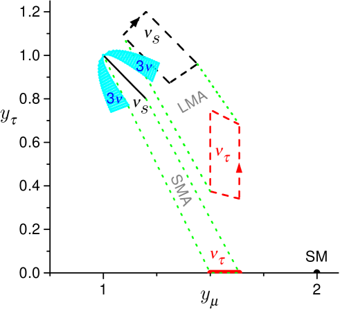
Figure 1: Predictions for the rates, $y_{\alpha}$, of AGN $\nu_{\mu}$, $\nu_{\tau}$ and $\nu_{e}$ fluxes at the Earth, normalized as $y_{e}+y_{\mu}+y_{\tau}=3$. The point ’SM’ corresponds to the no-mixing case. The solid segment labeled with $\nu_{s}$ ($\nu_{\tau}$) holds for a scenario with SMA solar $\nu_{e}-\nu_{s}$ ($\nu_{e}-\nu_{\tau}$) oscillations and atmospheric $\nu_{\mu}-\nu_{\tau}$ ($\nu_{\mu}-\nu_{s}$ ) oscillations. The areas enclosed by dashed lines are associated with large mixing angle ($\sin^{2}2\theta_{\odot}\geq 1/2$) solar neutrino solutions LMA, LOW or VO. The case of $\nu_{e}-\nu_{s}$ oscillations is labeled with $\nu_{s}$ and the case of $\nu_{e}-\nu_{\tau}$ oscillations is labeled with $\nu_{\tau}$. The regions limited by dotted lines correspond to the four-neutrino scenario where solar neutrinos oscillate to an arbitrary mixture of $\nu_{s}$ and $\nu_{\tau}$ which is decoupled from its orthogonal mixture by the LSND mass gap. The two triangular-like areas are predicted by the LMA three-neutrino scenario, with $\cos 2\theta_{\rm atm}<0$ in the upper ”triangle” and $\cos 2\theta_{\rm atm}>0$ in the lower one. In all cases $\sin^{2}2\theta_{\rm atm}$ varies from $0.8$ to $1$. The arrows indicate how $\sin^{2}2\theta_{\odot}$ grows from $1/2$ to $1$.

References

- [1] Y. Fukuda et al., Phys. Rev. Lett. 81 (1998) 1562, ibid. 82 (1999) 2644.
- [2] N. Hata and P. Langacker, Phys. Rev. D 56 (1997) 6107.
- [3] J. N. Bahcall, P. I. Krastev and A. Yu. Smirnov, Phys. Rev. D 58 (1998) 096016.
- [4] C. Athanassopoulos et al., Phys. Rev. Lett. 77 (1996) 3082; ibid. 81 (1998) 1774.
-
[5]
J. T. Peltoniemi and J. W. F. Valle, Nucl. Phys. B406 (1993) 409;
D. O. Caldwell and R. N. Mohapatra, Phys. Rev. D D48 (1993) 32. -
[6]
S. M. Bilenky, C. Giunti and W. Grimus, Eur. Phys. J. C1 (1998) 247;
V. Barger, T. J. Weiler and K. Whisnant, Phys. Lett. B427 (1998) 97;
V. Barger, S. Pakvasa, T. J. Weiler and K. Whisnant, Phys. Rev. D 58 (1998) 093016;
V. Barger, Y. Dai, K. Whisnant and B. Young, Phys. Rev. D 59 (1999) 113010. -
[7]
See the AMANDA homepage, http://amanda.berkeley.edu/;
the NESTOR homepage, http://www.roma1.infn.it/nestor/win97/espcrc2.html;
the BAIKAL homepage, http://www.ifh.de/baikal/baikalhome.html;
the ANTARES homepage, http://infodan.in2p3.fr/antares/;
the NEMO homepage, http://axplns.lns.infn.it/ neutrini/. -
[8]
See e.g. F. W. Stecker, C. Done, M. H. Salamon and P. Sommers,
Phys. Rev. Lett. 66 (1991) 2697; ibid. 69 (1992) 2738E;
F. W. Stecker and M. H. Salamon, Sp. Sci. Rev. 75 (1996) 341 (astro-ph/9501064);
M. C. Begelman, B. Rudak and M. Sikora, Ap. J. 362 (1990) 38. -
[9]
See e.g. P. L. Biermann and P. A. Strittmatter, Ap. J. 322 (1987) 643;
K. Mannheim, Astropart. Phys. 3 (1995) 295;
R. J. Protheroe, in Accretion Phenomena and Related Outflows, IAU colloquium 163, Volume 121 of the ASP conference series, ed. D. T. Wickramasinghe, G. V. Bicknell and L. Ferrario (Astronomical Society of the Pacific, San Francisco, 1997) (astro-ph/9607165). -
[10]
See e.g. J. P. Rachen and P. L. Biermann, Astron. Astrophys. 272 (1993) 161;
J. P. Rachen, T. Stanev and P. L. Biermann, Astron. Astrophys. 273 (1993) 377. -
[11]
See e.g. M. S. Longair, High Energy Astrophysics, Vol. I-II
(Cambridge University Press, Cambridge, 1994);
R. J. Protheroe, Topics in cosmic ray astrophysics, ed. M. A. DuVernois, Nova Science Publishing: New York, in press, 1999) (astro-ph/9812055). -
[12]
See e.g. T.K. Gaisser, F. Halzen and T. Stanev, Phys. Rep. 258 (1995) 175;
F. Halzen, Lectures presented at the TASI School, July 1998, astro-ph/9810368, and references therein. - [13] See R. Gandhi, C. Quigg, M. Reno and I. Sarcevic, Phys. Rev. D 58 (1998) 093009, and references therein.
- [14] J. G. Learned and S. Pakvasa, Astropart. Phys. 3 (1995) 267.
- [15] F. Halzen and D. Saltzberg, Phys. Rev. Lett. 81 (4305) 1998.
-
[16]
See e.g. P. Keränen, Phys. Lett. B417 (1998) 320;
G. Domokos and S. Kovesi-Domokos, Phys. Lett. B410 (1997) 57;
K. Enqvist, J. Maalampi and P. Keränen, Phys. Lett. B438 (1998) 295;
M. Roy and J. Wudka, Phys. Rev. D 56 (1997) 2403;
P. Keränen, J. Maalampi and J. T. Peltoniemi, Phys. Lett. B461 (1999) 230. -
[17]
J. N. Bahcall, P. I. Krastev and A. Yu. Smirnov, Phys. Rev. D 60 (1999) 093001;
M. C. Gonzalez-Garcia, P. C. de Holanda, C. Pena-Garay, J. W. F. Valle, preprint FTUV-99-41, (hep-ph/9906469). - [18] M. Apollonio et al., Chooz Coll., Phys. Lett. B420 (1998) 397.
-
[19]
R. Foot and R. R. Volkas, Phys. Rev. D 52 (1995) 6595;
W. Królikowski, Acta Phys. Polon. B30 (1999) 227 (hep-ph/9808307). -
[20]
R. Barbieri and A. Dolgov, Phys. Lett. B237 (1990) 440; Nucl. Phys. B237 (1991) 742;
K. Kainulainen, Phys. Lett. B244 (1990) 191;
K. Enqvist, K. Kainulainen and J. Maalampi, Phys. Lett. B249 (1990) 531;
Nucl. Phys. B349 (1991) 754. - [21] S. Burles, K. M. Nollett, J. N. Truran and M. S. Turner, Phys. Rev. Lett. 82 (1999) 4176.
- [22] X. Shi and G. M. Fuller, astro-ph/9904041 (1999).
-
[23]
See e.g. E. Lisi, S. Sarkar and F. L. Villante, Phys. Rev. D 59 (1999) 123520;
K. A. Olive, G. Steigman and T. P. Walker, astro-ph/9905320 (1999) (to be published in Phys. Rep.). -
[24]
See e.g. R. Foot, M. Thomson and R. R. Volkas, Phys. Rev. D 53 (1996) 5349;
R. Foot and R.R. Volkas, Phys. Rev. D 55 (1997) 5147;
X. Shi and G.M. Fuller, Phys. Rev. D 59 (1999) 063006;
P. Di Bari, P. Lipari and M. Lusignoli, hep-ph/9907548 (1999). - [25] R. M. Crocker, F. Melia and R. R. Volkas, preprint UM-P-99/40 (1999) (astro-ph/9911292).