CERN-TH/99-336

hep–ph/9911302

Thermal and Non-Thermal Production of Gravitinos in the Early Universe

G.F. Giudice^1,, A. Riotto^1, and I. Tkachev^2,

¹CERN Theory Division,

CH-1211 Geneva 23, Switzerland.

²Institut für Theoretische Physik, ETH-Hönggerberg, CH-8093, Zürich, Switzerland.

Abstract

The excessive production of gravitinos in the early universe destroys the successful predictions of nucleosynthesis. The thermal generation of gravitinos after inflation leads to the bound on the reheating temperature, $T_{RH}\stackrel{{\scriptstyle<}}{{{}_{\sim}}}10^{9}$ GeV. However, it has been recently realized that the non-thermal generation of gravitinos in the early universe can be extremely efficient and overcome the thermal production by several orders of magnitude, leading to much tighter constraints on the reheating temperature. In this paper, we first investigate some aspects of the thermal production of gravitinos, taking into account that in fact reheating is not instantaneous and inflation is likely to be followed by a prolonged stage of coherent oscillations of the inflaton field. We then proceed by further investigating the non-thermal generation of gravitinos, providing the necessary tools to study this process in a generic time-dependent background with any number of superfields. We also present the first numerical results regarding the non-thermal generation of gravitinos in particular supersymmetric models.

November 1999

1 Introduction

The overproduction of gravitinos represents a major obstacle in constructing cosmological models based on supergravity [25]. Gravitinos decay very late and – if they are copiously produced during the evolution of the early universe – their energetic decay products destroy the ⁴He and D nuclei by photodissociation, thus jeopardizing the successful nucleosynthesis predictions [2, 3]. As a consequence, the ratio of the number density of gravitinos $n_{3/2}$ to the entropy density $s$ should be smaller than about $10^{-12}$ [4] for gravitinos with mass of the order of 100 GeV.

Gravitinos can be produced in the early universe because of thermal scatterings in the plasma during the stage of reheating after inflation. To avoid the overproduction of gravitinos one has to require that the reheating temperature $T_{RH}$ after inflation is not larger than $\sim(10^{8}-10^{9})\>{\rm GeV}$ [3]. We will come back to this point and present a detailed analysis of the thermal generation of gravitinos during reheating.

However, it has been recently realized that the non-thermal effects occuring right after inflation because of the rapid oscillations of the inflaton field(s) provide an extra and very efficient source of gravitinos [5, 6]. The helicity $\pm 3/2$ part of the gravitino is excited only in tiny amounts, as the resulting abundance is always proportional to the gravitino mass $m_{3/2}$ [7]. On the contrary, the helicity $\pm 1/2$ part obeys the equation of motion of a normal helicity $\pm 1/2$ Dirac particle in a background whose frequency is a combination of the different mass scales at hand: the rapidly varying superpotential mass parameter of the fermionic superpartner of the scalar field whose $F$-term breaks supersymmetry, the Hubble rate and the gravitino mass [5, 6]. The non-thermal production of helicity $\pm 1/2$ gravitinos turns out to be much more efficient than their thermal generation during the reheat stage after inflation [5, 6] and it was claimed that the ratio $n_{3/2}/s$ for helicity $\pm 1/2$ gravitinos in generic supersymmetric models of inflation is roughly given by $10^{-2}T_{RH}/V^{1/4}$, where $V^{1/4}\sim 10^{15}$ GeV is the height of the potential during inflation. This leads to a very tight upper bound on the reheat temperature, $T_{RH}\stackrel{{\scriptstyle<}}{{{}_{\sim}}}10^{5}(V^{1/4}/10^{15}\>{\rm GeV})$ GeV [6].

The production of the helicity $\pm 1/2$ gravitino has been studied in refs. [5, 6] starting from the supergravity Lagrangian and in the simplest case in which the energy density and the pressure of the universe are dominated by an oscillating scalar field $\Phi$ belonging to a single chiral superfield with minimal kinetic term. An application in the context of supersymmetric new inflation models has been recently presented in ref. [8].

The equation describing the production of helicity $\pm 1/2$ gravitinos in supergravity reduces, in the limit in which the amplitude of the oscillating field is smaller than the Planck scale, to the equation describing the time evolution of the helicity $\pm 1/2$ Goldstino in global supersymmetry. This identification explains why there is no suppression by inverse powers of $M_{\rm P}$ in the final number density of helicity $\pm 1/2$ gravitinos and is a simple manifestation of the gravitino-Goldstino equivalence theorem: on-shell amplitudes with external helicity $\pm 1/2$ gravitinos are asymptotically equivalent to amplitudes with corresponding external Goldstinos for energies much larger than the gravitino mass [9]. This is analogous to the longitudinal $W$ bosons in the standard electroweak model behaving as Nambu-Goldstone bosons in the high energy limit.

This simple observation about the gravitino-Goldstino equivalence becomes crucial when the problem of computing the abundance of gravitinos generated by non-thermal effects involves more than one chiral superfield. Describing the production of helicity $\pm 1/2$ gravitinos through the equation of motion of the corresponding Goldstino in global supersymmetry is expected to provide the correct result in the case in which the scalar fields after inflation oscillate with amplitudes and frequencies smaller than the Planckian scale. Luckily, this situation is realized in most of the realistic supersymmetric models of inflation [10].

The goal of this paper is twofold. In the first part of this work we will still concern ourselves with some aspects of the thermal production of gravitinos during the reheating stage after inflation. We will perform a detailed analysis of such a process, taking into account the fact that reheating is far from being instantaneous. Inflation is followed by a prolonged stage of coherent oscillations of the inflaton field. In this regime, the inflaton is decaying, but the inflaton energy has not yet been entirely converted into radiation. The temperature $T$ rapidly increases to a maximum value and then slowly decreases as $a^{-3/8}$, being $a$ the scale factor of the universe. Only when the decay rate of the inflaton becomes of the order of the Hubble rate, the universe enters the radiation-dominated phase and one can properly define the reheat temperature $T_{RH}$. During this complicated dynamics, both gravitinos and entropy are continously generated and one has to solve a set of Boltzmann equations to compute the final ratio $n_{3/2}/s$.

In the second part of this work we will be dealing with the non-thermal production of gravitinos during the preheating stage after inflation.

Our aim is to provide the reader with all the tools necessary to study the helicity $\pm 1/2$ gravitino production in a generic time-dependent background and with a generic number of superfields. To achieve this goal, we will derive the master equation of motion of the Goldstino in global supersymmetry with a generic number of superfields and show that, in the case of one single chiral superfield and amplitudes of the oscillating fields smaller than the Planck scale, it exactly reproduces the equation of motion of the helicity $\pm 1/2$ gravitino found in refs. [5, 6] starting from the supergravity Lagrangian. As a special case, we will concentrate on the case of two chiral superfields, which is particularly relevant when dealing with supersymmetric models of hybrid inflation. We will also present the first complete numerical computation of the number density of the helicity $\pm 1/2$ gravitinos during the stage of preheating for one single chiral superfield. This numerical analysis will be performed keeping all the supergravity structure of the theory.

The paper is organized as follows. In sect. 2 we comment about the thermal production of gravitinos. In sect.  3, we show how to derive the equation of motion of the Goldstino in a generic time-dependent background, we reproduce the helicity $\pm 1/2$ gravitino equation found in supergravity for one single chiral superfield, we comment upon the decay rate of the helicity $\pm 1/2$ gravitinos and present the numerical results regarding the number density of gravitinos in particular supersymmetric models containing a single chiral superfield. Finally, in sect. 4 we discuss the non-thermal production of gravitinos for the case of two chiral superfields, which is relevant for realistic supersymmetric models of inflation.

2 Aspects of thermal production of gravitinos during reheating

At the end of inflation the energy density of the universe is locked up in a combination of kinetic energy and potential energy of the inflaton field, with the bulk of the inflaton energy density in the zero-momentum mode of the field. Thus, the universe at the end of inflation is in a cold, low-entropy state with few degrees of freedom, very much unlike the present hot, high-entropy universe. After inflation the frozen inflaton-dominated universe must somehow be defrosted and become a high-entropy radiation-dominated universe.

The process by which the inflaton energy density is converted to radiation is known as “reheating” [11]. The reader should rememeber that – even if the process of reheating is anticipated by a stage of preheating [12] – the efficiency of preheating is very sensitive to the model and the model parameters. In some models the process is inefficient; in some models it is not operative at all. Even if preheating is relatively efficient, it is unlikely that it removes all of the energy density of the inflaton field. In particular, already during the resonant decay of the inflaton field, back-reaction processes of rescattering [13] always create a sizeable population of inflaton quanta with non-zero momentum [14] which do not partecipate in the resonant decay. It is therefore likely that a stage during which the inflaton field is slowly decaying is necessary to extract the remaining inflaton field energy. This is exactly the stage we are going to analyze in this section.

The simplest way to envision this process is if the comoving energy density in the zero mode of the inflaton (or the soft quanta generated in the process of rescattering during preheating) decays into normal particles, which then scatter and thermalize to form a thermal background. It is usually assumed that the decay width of this process is the same as the decay width of a free inflaton field.

There are two reasons to suspect that the inflaton decay width might be small. The requisite flatness of the inflaton potential suggests a weak coupling of the inflaton field to other fields since the potential is renormalized by the inflaton coupling to other fields. However, this restriction may be evaded in supersymmetric theories where the nonrenormalization theorem ensures a cancelation between fields and their superpartners. A second and basic reason to suspect weak coupling is that in local supersymmetric theories gravitinos are produced during reheating. Unless reheating is delayed, gravitinos will be overproduced, leading to a large undesired entropy production when they decay after big-bang nucleosynthesis.

As we already mentioned, of particular interest is a quantity known as the reheat temperature, denoted as $T_{RH}$. In the oversimplified treatment, the reheat temperature is calculated by assuming an instantaneous conversion of the energy density in the inflaton field $\phi$ into radiation when the decay width of the inflaton energy, $\Gamma_{\phi}$, is equal to $H$, the expansion rate of the universe.

The reheat temperature is calculated quite easily [11]. After inflation the inflaton field $\phi$ executes coherent oscillations about the minimum of the potential. Averaged over several oscillations, the coherent oscillation energy density redshifts as matter: $\rho_{\phi}\propto a^{-3}$, where $a$ is the Robertson–Walker scale factor. If we denote as $\rho_{I}$ and $a_{I}$ the total inflaton energy density and the scale factor at the initiation of coherent oscillations, then the Hubble expansion rate as a function of $a$ is ($M_{Pl}=\sqrt{8\pi}M_{\rm P}$ is the Planck mass)

$$H^{2}(a)=\frac{8\pi}{3}\frac{\rho_{I}}{M^{2}_{Pl}}\left(\frac{a_{I}}{a}\right)^{3}.$$ (1)

Equating $H(a)$ and $\Gamma_{\phi}$ leads to an expression for $a_{I}/a$. Now if we assume that all available coherent energy density is instantaneously converted into radiation at this value of $a_{I}/a$, we can define the reheat temperature by setting the coherent energy density, $\rho_{\phi}=\rho_{I}(a_{I}/a)^{3}$, equal to the radiation energy density, $\rho_{R}=(\pi^{2}/30)g_{*}T_{RH}^{4}$, where $g_{*}$ is the effective number of relativistic degrees of freedom at temperature $T_{RH}$. The result is

$$T_{RH}=\left(\frac{90}{8\pi^{3}g_{*}}\right)^{1/4}\sqrt{\Gamma_{\phi}M_{Pl}}\ =0.2\left(\frac{200}{g_{*}}\right)^{1/4}\sqrt{\Gamma_{\phi}M_{Pl}}\ .$$ (2)

2.1 Thermal production of dangerous relics in the case of instantaneous reheating

Under the approximation of instantaneous reheating, the number density of any dangerous gravitational relic $X$ is readily solved. The Boltzmann equation reads

$$\frac{dn_{X}}{dt}+3Hn_{X}\simeq\langle\sigma_{{\rm tot}}|v|\rangle n^{2}_{{\rm light}},$$ (3)

where $\sigma_{{\rm tot}}\propto 1/M_{\rm P}^{2}$ is the total cross section determining the rate of production of the gravitational relic and $n_{{\rm light}}\sim T^{3}$ represents the number density of light particles in the thermal bath.

Since thermalization is by hypothesis very fast, the friction term $3Hn_{X}$ in Eq. (3) can be neglected and using the fact that the universe is radiation-dominated, i.e. $H\sim t^{-1}\sim T^{2}/M_{\rm P}$, one finds

$$n_{X}\propto\frac{T^{4}}{M_{\rm P}}.$$ (4)

The number density at thermalization in units of entropy density reads

$$\frac{n_{X}}{s}\simeq 10^{-2}\>\frac{T_{RH}}{M_{\rm P}}.$$ (5)

As mentioned in the introduction, the slow decay rate of the $X$-particles is the essential source of the cosmological problems because the decay products of the gravitational relics will destroy the ⁴He and D nuclei by photodissociation, and thus successful nucleosynthesis predictions. The most stringent bound comes from the resulting overproduction of D $+$ ³He, which would require that the relic abundance is smaller than $\sim 10^{-12}$ relative to the entropy density at the time of reheating after inflation [4]

$$\frac{n_{X}}{s}\stackrel{{\scriptstyle<}}{{{}_{\sim}}}10^{-12}.$$ (6)

Comparing Eqs. (6) and (5), one may obtain an upper bound on the reheating temperature after inflation [3]

$$T_{RH}\stackrel{{\scriptstyle<}}{{{}_{\sim}}}(10^{8}-10^{9})\>{\rm GeV}.$$ (7)

If $T_{RH}\sim M_{{\rm GUT}}$, dangerous relics such as gravitinos would be abundant during nucleosynthesis and destroy the good agreement of the theory with observations. However, if the reheating temperature satisfies the gravitino bound, it is too low to create superheavy GUT bosons that eventually decay and produce the baryon asymmetry [15].

In the discussion above, the crucial quantity which determines the abundance of dangerous relics after reheating is the reheat temperature $T_{RH}$ (or the inflaton decay rate $\Gamma_{\phi}$ through Eq. (2)). The reheat temperature is calculated by assuming an instantaneous conversion of the energy density in the inflaton field into radiation when the decay width of the inflaton energy is equal to the the expansion rate of the universe.

However, the reheating process is not instantaneous. Right after inflation the decay width of the inflaton is expected to be much smaller than the Hubble rate, $\Gamma_{\phi}\ll H$, otherwise $T_{RH}$ will violate the gravitino bound. Therefore, the universe undergoes a very long period of matter-domination during which the energy density is dominated by the oscillations of the inflaton field around the minimum of its potential. These oscillations last till the cosmic time becomes of the order of the lifetime of the inflaton field.

In this early-time and prolonged regime of inflaton oscillations, the inflaton is nevertheless decaying, $\rho_{\phi}\propto e^{-\Gamma_{\phi}t}$, but the inflaton energy has not yet been entirely converted into radiation. The temperature $T$ has the following behaviour. When the inflaton oscillations start and a small portion of the inflaton energy density has been transferred to radiation, the temperature rapidly grows to reach a maximum value $T_{MAX}$ and then it decreases scaling as $a^{-3/8}$, which implies that the entropy per comoving volume $S$ is created: $S\propto a^{15/8}$ [16, 11]. During this long stage, the universe is not yet radiation-dominated. Finally, when $t\sim\Gamma_{\phi}^{-1}$, the inflaton energy density gets converted entirely into radiation and the universe enters the radiation-dominated phase. Only at this point one can properly define the reheat temperature $T_{RH}$. Indeed, the reheat temperature is best regarded as the temperature below which the universe expands as a radiation-dominated universe, with the scale factor decreasing as $g_{*}^{-1/3}T^{-1}$, where $g_{*}$ is the number of relativistic degrees of freedom. In this regard it has a limited meaning [16, 11].

When studying the production of dangerous relics during reheating, it is necessary to take into account the fact that reheating is not instantaneous and that the maximum temperature is greater than $T_{RH}$. This implies that $T_{RH}$ should not be used as the maximum temperature obtained in the universe during reheating. The maximum temperature is, in fact, much larger than $T_{RH}$ and it is inconsistent to solve the Boltzmann equation for the gravitational relics assuming that throughout the period of reheating $n_{{\rm light}}\sim T^{3}\propto a^{-3}$ and that the reheat temperature $T_{RH}$ is the largest temperature of the thermal system after inflation. The goal of the next subsection is to provide a more appropriate computation of the number density of dangerous relics generated during the process of reheating. For sake of simplicity, we will focus on the gravitino case, but our results may be easily extended to other dangerous gravitational relics.

2.2 A more appropriate approach to thermal generation of gravitinos during reheating

Let us consider a model universe with three components: inflaton field energy, $\rho_{\phi}$, radiation energy density, $\rho_{R}$, and the number density of the gravitino, $n_{3/2}$. We will assume that the decay rate of the inflaton field energy density into radiation is $\Gamma_{\phi}$. We will also assume that the light degrees of freedom are in local thermodynamic equilibrium. This is by no means guaranteed, but the analysis performed in ref. [17] shows that, even if thermalization does not occur, production of gravitinos during reheating is not much different.

With the above assumptions, the Boltzmann equations describing the redshift and interchange in the energy density among the different components is

$$\dot{\rho}_{\phi}+3H\rho_{\phi}+\Gamma_{\phi}\rho_{\phi}=0,$$

$$\dot{\rho}_{R}+4H\rho_{R}-\Gamma_{\phi}\rho_{\phi}=0,$$

$$\dot{n}_{3/2}+3Hn_{3/2}+\langle\sigma_{{\rm tot}}|v|\rangle\left[n_{3/2}^{2}-\left(n_{3/2}^{EQ}\right)^{2}\right]=0,$$ (8)

where dot denotes time derivative. Here $\langle\sigma_{{\rm tot}}|v|\rangle$ is the total thermal average of the cross section times the Møller flux factor giving rise to the gravitino production and we have neglected the back-reaction of the gravitino abundance on the radiation energy density. The equilibrium energy density for the gravitinos, $n_{3/2}^{EQ}$, is determined by the radiation temperature, $T$.

It is useful to introduce two dimensionless constants, $\alpha_{\phi}$ and $\alpha_{X}$, defined in terms of $\Gamma_{\phi}$ and $\langle\sigma|v|\rangle$ as

$$\Gamma_{\phi}=\alpha_{\phi}M_{\phi}\qquad\langle\sigma|v|\rangle=\alpha_{X}m_{3/2}^{-2}\ .$$ (9)

For a reheat temperature much smaller than $M_{\phi}$, $\Gamma_{\phi}$ must be small. From Eq. (2), the reheat temperature in terms of $\alpha_{\phi}$ and $M_{\phi}$ is $T_{RH}\simeq\alpha_{\phi}^{1/2}\sqrt{M_{\phi}M_{Pl}}$. For $M_{\phi}=10^{13}$ GeV, $\alpha_{\phi}$ must be approximately smaller than $10^{-13}$.

It is also convenient to work with rescaled quantities that can absorb the effect of expansion of the universe. This may be accomplished with the definitions

$$\Phi\equiv\rho_{\phi}M_{\phi}^{-1}a^{3}\ ;\quad R\equiv\rho_{R}a^{4}\ ;\quad X\equiv n_{3/2}a^{3}\ .$$ (10)

It is also convenient to use the scale factor, rather than time, for the independent variable, so we define a variable $x=aM_{\phi}$. With this choice the system of equations (2.2) can be written as (prime denotes $d/dx$)

$$\Phi^{\prime} = -c_{1}\ \frac{x}{\sqrt{\Phi x+R}}\ \Phi,$$

$$R^{\prime} = c_{1}\ \frac{x^{2}}{\sqrt{\Phi x+R}}\ \Phi,$$

$$X^{\prime} = -c_{3}\ \frac{x^{-2}}{\sqrt{\Phi x+R}}\ \left(X^{2}-X_{EQ}^{2}\right).$$ (11)

The constants $c_{1}$, $c_{2}$, and $c_{3}$ are given by

$$c_{1}=\sqrt{\frac{3}{8\pi}}\frac{M_{Pl}}{M_{\phi}}\alpha_{\phi}\ \qquad c_{2}=c_{1}\frac{M_{\phi}}{M_{X}}\frac{\alpha_{X}}{\alpha_{\phi}}\ \qquad c_{3}=\sqrt{\frac{3}{8\pi}}\alpha_{X}\frac{M_{Pl}M_{\phi}}{m_{3/2}^{2}}\ .$$ (12)

$X_{EQ}$ is the equilibrium value of $X$, given in terms of the temperature $T$ as

$$X_{EQ}=\frac{3}{4}\frac{\zeta(3)}{\pi^{2}}g_{3/2}x^{3}\left(\frac{T}{M_{\phi}}\right)^{3}\ .$$ (13)

The temperature depends upon $R$ and $g_{*}$, the effective number of degrees of freedom in the radiation:

$$T=\left(\frac{30}{g_{*}\pi^{2}}\right)^{1/4}M_{\phi}\frac{R^{1/4}}{x}\ .$$ (14)

It is straightforward to solve the system of equations in Eq. (2.2) with initial conditions at $x=x_{I}$ of $R(x_{I})=X(x_{I})=0$ and $\Phi(x_{I})=\Phi_{I}$. It is convenient to express $\rho_{\phi}(x=x_{I})$ in terms of the expansion rate at $x_{I}$, which leads to

$$\Phi_{I}=\frac{3}{8\pi}\frac{M^{2}_{Pl}}{M_{\phi}^{2}}\frac{H_{I}^{2}}{M_{\phi}^{2}}\ x_{I}^{3}\ .$$ (15)

Before numerically solving the system of equations, it is useful to consider the early-time solution for $R$. Here, by early time, we mean $H\gg\Gamma_{\phi}$, i.e., before a significant fraction of the comoving coherent energy density is converted to radiation. At early times $\Phi\simeq\Phi_{I}$, and $R\simeq X\simeq 0$, so the equation for $R^{\prime}$ becomes $R^{\prime}=c_{1}x^{3/2}\Phi_{I}^{1/2}$. Thus, the early time solution for $T$ is simple to obtain [17]

$$\frac{T}{M_{\phi}}\simeq\left(\frac{12}{\pi^{2}g_{*}}\right)^{1/4}c_{1}^{1/4}\left(\frac{\Phi_{I}}{x_{I}^{3}}\right)^{1/8}\left[\left(\frac{x}{x_{I}}\right)^{-3/2}-\left(\frac{x}{x_{I}}\right)^{-4}\right]^{1/4}\qquad(H\gg\Gamma_{\phi})\ .$$ (16)

Thus, $T$ has a maximum value of

$$\frac{T_{MAX}}{M_{\phi}} = 0.77\left(\frac{12}{\pi^{2}g_{*}}\right)^{1/4}c_{1}^{1/4}\left(\frac{\Phi_{I}}{x_{I}^{3}}\right)^{1/8}$$ (17)

$$= 0.77\alpha_{\phi}^{1/4}\left(\frac{9}{2\pi^{3}g_{*}}\right)^{1/4}\left(\frac{M_{Pl}^{2}H_{I}}{M_{\phi}^{3}}\right)^{1/4}\ ,$$

which is obtained at $x/x_{I}=(8/3)^{2/5}=1.48$. It is also possible to express $\alpha_{\phi}$ in terms of $T_{RH}$ and obtain

$$\frac{T_{MAX}}{T_{RH}}=0.77\left(\frac{9}{5\pi^{3}g_{*}}\right)^{1/8}\left(\frac{H_{I}M_{Pl}}{T_{RH}^{2}}\right)^{1/4}\ .$$ (18)

For an illustration, in the simplest model of chaotic inflation $H_{I}\sim M_{\phi}$ with $M_{\phi}\simeq 10^{13}$ GeV, which leads to $T_{MAX}/T_{RH}\sim 10^{3}(200/g_{*})^{1/8}$ for $T_{RH}=10^{9}$ GeV.

For $x/x_{I}>1$, in the early-time regime $T$ scales as $a^{-3/8}$, which implies that entropy is created in the early-time regime [16]. So if one is producing gravitinos during reheating it is necessary to take into account the fact that the maximum temperature is greater than $T_{RH}$, and that during the early-time evolution, $T\propto a^{-3/8}$.

The equation of motion of the number density of the gravitino is easily solved numerically. The results are plotted in Fig. 1. The total cross section for the gravitino production is such that $\alpha_{X}\simeq 16.6(m_{3/2}/M_{\rm P})^{2}$ while the total number of relativistic degrees of freedom is $g_{*}\simeq 230$. The inflaton parameters have been chosen to have $T_{RH}=10^{9}$ GeV, which gives $T_{MAX}\simeq 10^{12}$ GeV.

Figure 1: The time dependence of the temperature, the radiation energy density, the inflaton energy density and the gravitino number density for the case $T_{RH}=10^{9}$ GeV

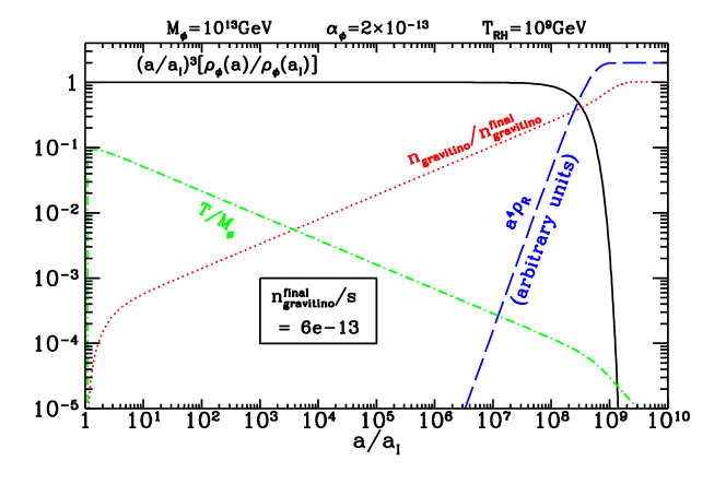
We observe that the quantity $(n_{3/2}/s)/(n_{3/2}/s)_{{\rm final}}$, where $s$ is the entropy density, gradually increases with time when $\Gamma_{\phi}$ is smaller than $H$, but remains always smaller than unity until the inflaton decays at $t\sim\Gamma_{\phi}^{-1}$. This means that most of the gravitinos are produced at the last stage of reheating when the inflaton decays and it makes sense to talk about $T_{RH}$. We have also checked that $(n_{3/2}/s)_{{\rm final}}$ approximates well the usual estimate one gets neglecting the non-trivial evolution of the temperature of the radiation during the period $\Gamma_{\phi}\ll H$. This result can be explained recalling that – during the coherent oscillation epoch – the entropy per comoving volume is increasing and the abundance of the just-produced gravitinos is continuously diluted by the entropy release. We have also checked that the final number density of gravitinos has a dependence, even though weak, on the frequency of the inflaton oscillations $M_{\phi}$. This dependence is not present in the case of instantaneous reheating, where the number density of gravitinos depends only upon the reheating temperature and not on the frequency of the inflaton oscillations.

We conclude that – even though the maximum temperature of $10^{12}$ GeV seems to be in contradiction with the usually quoted upper bound of $(10^{9}-10^{10})$, imposing the constraint (6) gives the usual upper bound on the reheating temperature $T_{RH}\stackrel{{\scriptstyle<}}{{{}_{\sim}}}10^{9}$ GeV. One should keep in mind, however, that the thermal evolution of the universe before the epoch $t\sim\Gamma_{\phi}^{-1}$ is nonstandard and the physics leading to the bound $T_{RH}\stackrel{{\scriptstyle<}}{{{}_{\sim}}}10^{9}$ GeV is much more involved than is usually thought. This observation might be relevant when dealing with either a different parameter space for the gravitino, e.g. if the gravitino is very light, or with other kinds of dangerous relics.

3 Non-thermal production of gravitinos and the gravitino-Goldstino equivalence

As shown in refs. [5, 6], non-thermal effects occuring right after inflation due to the rapid oscillations of the inflaton field(s) may lead to copious gravitino production. As we noted in the introduction, this occurs because the helicity $\pm 1/2$ part of the gravitino can be efficiently excited during the evolution of the Universe after inflation. The non-thermal generation can be extremely efficient and overcome the thermal production by several orders of magnitude, in realistic supersymmetric inflationary models.

The equation of the helicity $\pm 1/2$ gravitino has been found in refs. [5, 6] in the case in which the energy density and the pressure of the universe are dominated by an oscillating scalar field $\Phi$ belonging to a single chiral superfield with minimal kinetic term. In this section we would like to study the non-thermal production of gravitinos in a generic time-dependent gravitational background and for a generic number of chiral superfields.

The equation of the helicity $\pm 1/2$ gravitino with a single chiral superfield and minimal kinetic term is identical to the familiar equation for a spin-1/2 fermion in a time-varying background with frequency $\Omega$, which depends upon all the mass scales appearing in the problem, namely the Goldstino mass parameter $\partial_{\Phi}^{2}W$ (where $W(\Phi)$ denotes the superpotential), the Hubble rate $H$ and the gravitino mass $m_{3/2}$. In the limit in which the amplitude of the oscillating scalar field is small, $|\Phi|\ll M_{\rm P}$, the frequency of the oscillations tends to $\partial_{\Phi}^{2}W$. The frequency $\Omega$ corresponds to the superpotential mass parameter of the Goldstino which is ‘eaten’ by the gravitino when supersymmetry is broken. Therefore, the equation describing the production of helicity-1/2 gravitinos in supergravity reduces, in the limit of $|\Phi|\ll M_{\rm P}$, to the equation describing the time evolution of the helicity-1/2 Goldstino in global supersymmetry and no suppression by powers of $M_{\rm P}$ is present.

This does not come as a surprise and is in agreement with the gravitino-Goldstino equivalence theorem. In spontaneously broken supergravity, the initially massless gravitino acquires a mass through the superhiggs mechanism [18, 19], by absorbing the Goldstino which disappears from the physical spectrum. Before becoming massive, the gravitino, which is a Majorana spin $3/2$ particle, posseses only $\pm 3/2$ helicity states. The Goldstino, a Majorana fermion, provides for its missing (longitudinal) $\pm 1/2$ states. The equivalence theorem is valid in the limit of large energies compared to $m_{3/2}$ where the longitudinal component of the gravitino effectively behaves as a spin $1/2$ Goldstino [9].

Therefore, it appears of advantage to compute the equation of motion of the helicity $\pm 1/2$ gravitino by finding the equation of motion of the corresponding Goldstino in global supersymmetry. This procedure is particularly welcome when the problem involves more than one chiral superfield and is expected to provide the correct result for the number density of helicity $\pm 1/2$ gravitinos in the case in which the scalar fields after inflation oscillate with amplitudes and frequencies smaller than the Planckian scale. This is exactly what is realized in most of the realistic supersymmetric models of inflation [10].

3.1 The equation of motion of the Goldstino in global supersymmetry and in a time-dependent background

Let us now find the equation of motion of the Goldstino when the energy density of the background is dominated by a set of scalar fields following the trajectories imposed by their equation of motion. We will therefore suppose that the scalar fields are displaced from the minima of their potential and are free to oscillate about such minima. This is what happens right after inflation and during the preheating stage.

The identification of the Goldstino requires a generalization of the standard procedure used in the static case, that is when the scalar fields are sitting at the minima of their potential and the cosmological constant vanishes. In the following we will neglect the expansion of the universe. For the practical purpose of computing the number density of helicity $\pm 1/2$ gravitinos generated during the preheating stage, this is good approximation since the non-thermal production of gravitinos is expected to overcome the thermal generation in those supersymmetric models in which the frequency of the oscillations of the scalar fields is much larger than the rate of the expansion of the universe and most of the gravitinos are generated within the first few oscillations. Neglecting the expansion of the universe will also make the identification of the Goldstino more transparent. Finally, we will not concern ourselves with a theory charged under some gauge group, but suppose that during the evolution of the system some $F$-term is nonvanishing. Our findings can be easily generalized to include the possibility that supersymmetry is broken by some (time-dependent) $D$-term.

Consider a global supersymmetric theory with Lagrangian

$${\cal L}=\partial_{\mu}z_{i}\partial^{\mu}z^{i}+\frac{i}{2}\bar{\chi}_{i}\gamma_{\mu}\partial^{\mu}\chi_{i}-V(z^{i},z_{i})-\frac{1}{2}\left(W_{ij}\bar{\chi}_{i}P_{L}\chi^{j}+{\rm h.c.}\right),$$

$$V(z^{i},z_{i})=W_{i}(W^{\dagger})^{i}.$$ (19)

Here $W=W(z^{i})$ is the superpotential, $z^{i}$ and $\chi_{i}$ denote a set the scalar and fermionic fields respectively, $z_{i}=(z^{i})^{\dagger}$, $W_{i}=\partial W/\partial z^{i}$ and $P_{L}=(1-\gamma_{5})/2$ is the left-handed projection operator. The index $i$ runs from 1 to $N$, being $N$ the number of multiplets and we use the standard convention that the sum is intended when the index $i$ is contracted.

The Lagrangian is invariant under the following set of supersymmetric transformations

$$\delta_{\varepsilon}z^{i} = \sqrt{2}\bar{\varepsilon}P_{L}\chi^{i},$$

$$\delta_{\varepsilon}\chi^{i} = \sqrt{2}\Theta^{i}\varepsilon,$$ (20)

where $\varepsilon$ is the spinor parametrizing the infinitesimal supersymmetric transformation and we have defined the matrix

$$\Theta^{i}=\left[i\partial\hbox to0.0pt{\hss/}z^{i}-(W^{\dagger})^{i}\right].$$ (21)

Given a generic background, supersymmetry is broken if

$$\langle\delta_{\varepsilon}\chi^{i}\rangle\neq 0.$$ (22)

This happens if the expectation value of the matrix $\Theta^{i}$ is nonvanishing

$$\langle\Theta^{i}\rangle\neq 0.$$ (23)

In particular, for a constant (time-independent) background, one recovers the usual condition that supersymmetry is broken if, for some field $z^{i}$, the $F$-term is nonvansishing

$$\langle W_{i}\rangle\neq 0.$$ (24)

On the other hand, in the case of a time-dependent background, the breakdown of supersymmetry comes also from the

$$\gamma_{0}\frac{dz^{i}}{dt}$$ (25)

piece in the matrix $\Theta^{i}$. This is not surprising since supersymmetry is broken in the early universe anytime some form of nonvanishing energy density appears. This is what happens during inflation and the subsequent stage of preheating and reheating when scalar fields oscillate around the minima of their potential.

The Goldstone theorem tells us that the Goldstino is easily identified from the supersymmetric transformation (3.1)

$$\eta=\Theta_{i}\chi_{i}.$$ (26)

We introduce now the two projection operators

$$(P^{\perp})_{ij} = \delta_{ij}-\frac{\Theta^{\dagger}_{i}}{\Theta^{\dagger}\Theta}\Theta_{j},$$

$$(P^{\parallel})_{ij} = \frac{\Theta^{\dagger}_{i}}{\Theta^{\dagger}\Theta}\Theta_{j},$$ (27)

where we have defined $\Theta^{\dagger}\Theta=\Theta_{k}^{\dagger}\Theta_{k}$. The two operators project respectively onto the subspace orthogonal to the Goldstone fermion and onto the Goldstone fermion itself.

Making use of the definition (21), we find that, for a background of real fields,

$$\Theta^{\dagger}\Theta=\sum_{i}\left[\left(\frac{dz^{i}}{dt}\right)^{2}+\left(W_{i}\right)^{2}\right]=\rho.$$ (28)

Therefore, the combination $\Theta^{\dagger}\Theta$ gives the total energy density of the system $\rho$ which – if the expansion of the universe is neglected – remains constant in time.

The spin $1/2$ field $\chi_{i}$ can be rewritten as

$$\chi_{i} = \chi_{i}^{\perp}+\frac{\Theta^{\dagger}_{i}}{\Theta^{\dagger}\Theta}\eta,$$

$$\chi_{i}^{\perp} = (P^{\perp})_{ij}\chi_{j}.$$ (29)

Notice that the fields $\chi_{i}^{\perp}$ are not linearly independent since they satisfy the following relation

$$\Theta_{i}\chi_{i}^{\perp}=0.$$ (30)

This condition tells us that one of the $\chi_{i}^{\perp}$ fields may be expressed in terms of the remaining $(N-1)$ ones.

We now choose the nonvanishing vacuum expectation values of the scalar fields in the real direction, ${\rm Re}\>z_{i}=\phi_{i}/\sqrt{2}$, ${\rm Im}\>z_{i}=0$. The equation of motion of the scalar and fermionic fields read

$$\ddot{\phi_{i}} = -W_{ij}W_{j},$$ (31)

$$i\gamma^{0}\dot{\chi}_{i} = \hat{k}\chi_{i}+W_{ij}\chi_{j},$$ (32)

where the dots stand for derivative with respect to time, $\hat{k}=\vec{\gamma}\cdot\vec{k}$ and we have used the plane-wave ansatz $\chi_{i}\sim e^{i\vec{k}\cdot\vec{x}}$ for the space-dependent part. The matrices $\Theta_{i}$ satisfy the following equation

$$i\gamma^{0}\dot{\Theta}_{i}=-W_{ij}\Theta_{j}.$$ (33)

Inserting now the decomposition (3.1) into Eq. (32), multiplying by $\Theta_{i}$ and $\Theta_{i}^{\dagger}$ respectively and making use of the Eq. (33), we get the following equations of motion

$$i\gamma^{0}\dot{\eta} = \hat{k}{\cal G}^{\dagger}\eta+\hat{k}\hat{\chi},$$ (34)

$$i\gamma^{0}\dot{\hat{\chi}} = -i{\cal G}^{\dagger}\gamma^{0}\dot{\eta}+\hat{k}\eta+2\Theta_{i}^{\dagger}W_{ij}\chi^{\perp}_{j},$$ (35)

where we have defined the following combinations

$${\cal G} = \frac{\Theta_{i}\Theta_{i}}{\Theta^{\dagger}\Theta},$$

$$\hat{\chi} = \Theta_{i}^{\dagger}\chi^{\perp}_{i}.$$ (36)

The matrix ${\cal G}$ can be expressed in terms of the energy density $\rho$ and the pressure $p$ of the oscillating scalar fields

$${\cal G}=-\frac{p+2i\gamma^{0}\dot{W}}{\rho}.$$ (37)

Differentiating Eq. (34) with respect to time and using Eq. (35) we find the master equation of motion of the Goldstino

$$\ddot{\eta}+k^{2}\eta+i\gamma^{0}\hat{k}\dot{{\cal G}}^{\dagger}\eta-2i\hat{k}\gamma^{0}\dot{\Theta}_{i}^{\dagger}\chi^{\perp}_{i}=0.$$ (38)

This equation is valid for a generic number of chiral superfields and – because of the gravitino-Goldstino equivalence theorem – is expected to provide the necessary tool to describe the production of helicity $\pm 1/2$ gravitinos during the preheating stage after inflation, when the typical energy of the system and field amplitudes (or the frequencies of the oscillations of the scalar fields) are large compared to the gravitino mass $m_{3/2}$ and smaller than the Planck scale. We notice the non-trivial result that any time-dependent function has disappeared from the $k^{2}\eta$ term; in the ultraviolet regime, Eq. (38) is solved by plane-waves and particle production shuts off as one would expect from general arguments.

In a static background for which $\dot{\phi}_{i}=0$, we have $\Theta_{i}=\Theta_{i}^{\dagger}$, $\dot{G}^{\dagger}=\dot{\Theta}_{i}=0$ and $\hat{\chi}=0$ by virtue of Eq. (30). The Goldstino equation is solved by plane-waves and – as expected – no particle production takes place.

Let us now consider the special case of one single chiral superfield $\Phi$ with minimal kinetic term. We have $N=1$, the only physical degree of freedom is the Goldstino and

$$\chi^{\perp}=\hat{\chi}=0.$$ (39)

Eq. (34) simplifies to

$$\left(i\gamma^{0}\partial_{0}-\hat{k}{\cal G}^{\dagger}\right)\eta=0,$$ (40)

where

$${\cal G}=\frac{\Theta_{1}}{\Theta_{1}^{\dagger}},$$ (41)

and the matrix $\Theta_{1}$ is given in Eq. (21) for the case $i=1$. Notice that the matrix ${\cal G}$ has manifestly absolute value equal to unity

$$\left|{\cal G}\right|^{2}={\cal G}^{\dagger}{\cal G}=\frac{\Theta_{1}^{\dagger}}{\Theta_{1}}\times\frac{\Theta_{1}}{\Theta_{1}^{\dagger}}={\bf 1}.$$ (42)

Therefore, it is possible to rewrite ${\cal G}$ in the following form

$${\cal G}=e^{2i\gamma^{0}\varphi},$$ (43)

By making a field redifinition $\eta\rightarrow{\rm exp}(i\gamma^{0}\varphi)\eta$, the equation of motion of the Goldstino becomes

$$i\gamma^{0}\dot{\eta}-\hat{k}\eta-m_{{\rm eff}}\eta=0,$$ (44)

where

$$m_{{\rm eff}}=\dot{\varphi}=\frac{\partial^{2}W}{\partial\Phi^{2}}$$ (45)

and we have used the fact that ${\cal G}$ satisfies the following differential equation

$$\frac{\dot{{\cal G}}}{{\cal G}}=2i\gamma^{0}\frac{\partial^{2}W}{\partial\Phi^{2}}.$$ (46)

Eq. (44) is the equation of motion of a spin-1/2 fermion in a time-dependent background given by the oscillating mass $m_{{\rm eff}}$. We now wish to show that the Eq. (44) found for one single chiral superfield in the limit of global supersymmetry correctly reproduces – for amplitudes of the scalar field $\Phi$ much smaller than the Planck scale – the equation of motion of the helicity $\pm 1/2$ gravitino found in refs. [5, 6] starting from a local supersymmetric theory, i.e. supergravity.

3.2 Non-thermal production of gravitinos in the case of one chiral superfield

Let us first remind the reader of some of the basic results obtained in refs. [5, 6] regarding the equation of motion of the helicity $\pm 1/2$ gravitino in the case of one single chiral superfield and minimal kinetic term.

If we start with the supergravity Lagrangian, the single chiral fermion $\chi$ – which is the superpartner of the scalar component in the chiral supermultiplet $\Phi$ – plays the role of the Goldstino and can be gauged away to zero, so that no mixing between the gravitino $\psi_{\mu}$ and $\chi$ is present. Under these circumnstances, the equation of motion of the gravitino becomes

$$R^{\mu}\equiv\epsilon^{\mu\nu\rho\sigma}\gamma_{5}{\hat{\gamma}}_{\nu}{\cal D}_{\rho}\psi_{\sigma}=0.$$ (47)

Here ${\cal D}_{\rho}$ is the covariant derivative and greek letters denote space-time indices. The condition ${\cal D}\cdot R=0$ gives the following algebraic constraint

$$\hat{\gamma}_{0}\psi^{0}=c\sum_{i=1}^{3}{\hat{\gamma}}_{i}\psi^{i},$$ (48)

where the matrix $c$, in the limit of $|\Phi|\ll M_{\rm P}$, reduces to

$$c=\frac{p+2i\gamma^{0}\dot{W}}{\rho}=-{\cal G}.$$

Two degrees of freedom may be eliminated using Eq. (48).

We note that the constraint (48) may be recovered in the following alternative way. The mixing term in the supergravity Lagrangian between the gravitino and the Goldstino is of the form

$$\bar{\chi}{\hat{\gamma}}^{\mu}\Theta_{1}^{\dagger}\psi_{\mu}.$$ (49)

By using the definition (26) $\eta=\Theta_{1}\chi$ the mixing term becomes

$$\frac{1}{\Theta_{1}^{\dagger}\Theta_{1}}\bar{\eta}\Theta_{1}{\hat{\gamma}}^{\mu}\Theta_{1}^{\dagger}\psi_{\mu}.$$ (50)

Choosing the gauge in which such a term vanishes is equivalent to require that

$$\Theta_{1}{\hat{\gamma}}^{\mu}\Theta_{1}^{\dagger}\psi_{\mu}=0.$$ (51)

This condition gives $\hat{\gamma}_{0}\psi^{0}=-{\cal G}\sum_{i=1}^{3}{\hat{\gamma}}_{i}\psi^{i}$, which coincides with the constraint (48).

Because of the antisymmetric properties of the Levi-Civita symbol, the equation $R^{0}=0$ does not contain time derivatives and provides another algebraic constraint on the gravitino momentum modes. Such a constraint allows to remove two extra degrees of freedom and to define two physical Majorana fermion states $\psi_{3/2}$ and $\psi_{1/2}$ which may be shown to correspond to the $\pm 3/2$ and $\pm 1/2$ helicity states respectively, by explicitly constructing the helicity projectors in the flat limit [6]. The Lagrangian may be diagonalized as [6] ${\cal L}={\cal L}_{3/2}+{\cal L}_{1/2}$, where

$${\cal L}_{3/2} = \bar{\psi}_{3/2}\left[i\gamma^{0}\partial_{0}+i\frac{5\dot{a}}{2a}\gamma^{0}-m_{3/2}a\right]\psi_{3/2},$$

$${\cal L}_{1/2} = \bar{\psi}_{1/2}\left[i\gamma^{0}\partial_{0}+i\frac{5\dot{a}}{2a}\gamma^{0}+m_{3/2}a+\hat{k}G\right]\psi_{1/2},$$ (52)

where $a$ is the scale factor, $G=A+i\gamma^{0}B$ and $A$ and $B$ are time-dependent functions [6]

$$A = \frac{1}{3\left(\frac{\dot{a}^{2}}{a^{4}}+m_{3/2}^{2}\right)^{2}}\left[2\frac{\ddot{a}}{a^{3}}\left(m_{3/2}^{2}-\frac{\dot{a}^{2}}{a^{4}}\right)+\frac{\dot{a}^{4}}{a^{8}}-4m_{3/2}^{2}\frac{\dot{a}^{2}}{a^{4}}+3m_{3/2}^{4}\right.$$ (53)

$$- \left.4\frac{\dot{a}}{a^{3}}\dot{m}_{3/2}m_{3/2}\right],$$

$$B = \frac{2m_{3/2}}{3\left(\frac{\dot{a}^{2}}{a^{4}}+m_{3/2}^{2}\right)^{2}}\left[2\frac{\ddot{a}\dot{a}}{a^{5}}-\frac{\dot{a}^{3}}{a^{6}}+3m_{3/2}^{2}\frac{\dot{a}}{a^{2}}+\frac{\dot{m}_{3/2}}{m_{3/2}a}\left(m_{3/2}^{2}-\frac{\dot{a}^{2}}{a^{4}}\right)\right].$$ (54)

They may be expressed in terms the pressure and the energy density of the scalar field $\Phi$. Here time is conformal and the line element is $ds^{2}=a^{2}(\tau)(d\tau^{2}-d{\vec{x}}^{2})$.

The diagonal time and space components of the Einstein equation become

$$\frac{\dot{a}^{2}}{a^{4}} = \frac{1}{3M_{\rm P}^{2}}\left[V(\Phi)+\left|\frac{d\Phi}{dt}\right|^{2}\right],$$ (55)

$$2\frac{\ddot{a}}{a^{3}}-\frac{\dot{a}^{2}}{a^{4}} = \frac{1}{M_{\rm P}^{2}}\left[V(\Phi)-\left|\frac{d\Phi}{dt}\right|^{2}\right].$$ (56)

Using the expression for the gravitino mass $m_{3/2}$ in terms of the superpotential $W$,

$$m_{3/2}=e^{\frac{\Phi^{\dagger}\Phi}{2M_{\rm P}^{2}}}~{}\frac{|W(\Phi)|}{M_{\rm P}^{2}},$$ (57)

we can write the scalar potential $V$ as

$$V=e^{\frac{\Phi^{\dagger}\Phi}{M_{\rm P}^{2}}}\left[\left|\partial_{\Phi}W+\frac{\Phi^{\dagger}W}{M_{\rm P}^{2}}\right|^{2}-\frac{3|W|^{2}}{M_{\rm P}^{2}}\right]=m_{3/2}^{2}M_{\rm P}^{2}\left[\left|\frac{\dot{m}_{3/2}M_{\rm P}}{am_{3/2}\frac{d\Phi}{dt}}\right|^{2}-3\right].$$ (58)

Replacing Eqs. (55) and (56) in Eq. (58), one obtains [6]

$$\dot{m}_{3/2}^{2}=-\frac{\ddot{a}^{2}}{a^{4}}+\frac{\ddot{a}}{a}\left(\frac{\dot{a}^{2}}{a^{4}}-3m_{3/2}^{2}\right)+2\frac{\dot{a}^{4}}{a^{6}}+6\frac{\dot{a}^{2}}{a^{2}}m_{3/2}^{2}.$$ (59)

When this expression for $\dot{m}_{3/2}$ is used in Eqs. (53) and (54), we obtain the ramarkable property [5, 6]

$$\left|G^{\dagger}G\right|=A^{2}+B^{2}=1.$$ (60)

We are now in the position to show the gravitino-Goldstino equivalence explicitly. To do so, we neglect the expansion of the universe and the gravitino mass $m_{3/2}$ and consider the limit $|\Phi|\ll M_{\rm P}$. The matrix $G$ has the following limit [5, 6]

$$G\stackrel{{\scriptstyle|\Phi|\ll M_{\rm P}}}{{\longrightarrow}}\frac{p-2i\gamma^{0}\dot{W}}{\rho}=-{\cal G}^{\dagger}.$$ (61)

The equation of motion of the helicity $\pm 1/2$ gravitino therefore reduces to

$$\left(i\gamma^{0}\partial_{0}-\hat{k}{\cal G}^{\dagger}\right)\psi_{1/2}=0.$$ (62)

This equation is exactly reproduced in the global supersymmetric limit by the equation of motion of the Goldstino (40).

One can also use the gravitino-Goldstino equivalence to explain the remarkable property that the matrix $G$ has absolute value equal to unity, by making use of Eq. (42).

3.3 Comments on the gravitino decay

We bragged about achieving a large number density of helicity $\pm 1/2$ gravitinos from non-thermal effects and how this phenomenon is strictly related to the fact that $M_{\rm P}$ does not appear in the equation of motions, but then tacitly assumed that the comoving number of helicity $\pm 1/2$ gravitinos at nucleosynthesis is the same one which may be generated during preheating. This issue deserves a closer look because one might think that helicity $\pm 1/2$ gravitinos promptly decay (or rapidly thermalize), thus not leading to a large undesired entropy production when they decay after big-bang nucleosynthesis.

However, this is not the case; helicity $\pm 1/2$ gravitinos do have a decay rate which is suppressed by the gravitational coupling $M_{\rm P}^{-2}$ and is therefore small. This can be easily understood in the following way. The helicity $\pm 1/2$ components of the gravitino field correspond to the Goldstino, which is derivatively coupled to the supercurrent. Hence, the total amplitude for the decay rate of the helicity $\pm 1/2$ gravitino has to be proportional to the mass splitting within the supermultiplets. For example, in the present vacuum, where we suppose supersymmetry is broken by some $F$-term with $F\sim m_{3/2}M_{\rm P}$, the coupling between the helicity $\pm 1/2$ gravitino, a fermion $f$ and its superpartner $\widetilde{f}$ is proportional to $(m^{2}_{\widetilde{f}}-m_{f}^{2})/F$. Since $(m^{2}_{\widetilde{f}}-m_{f}^{2})\sim m_{3/2}^{2}$, the coupling is suppressed by $m_{3/2}/M_{\rm P}^{-1}$. Similarly, the coupling of the helicity $\pm 1/2$ gravitino, with a gauge boson and a gaugino is proportional to $m_{\lambda}/F\sim M_{\rm P}^{-1}$, where $m_{\lambda}\sim m_{3/2}$ is the gaugino mass. This is the reason why, when dealing with thermal production of gravitinos during reheating, the helicity $\pm 1/2$ and $\pm 3/2$ gravitinos are treated on the same ground and have both $M_{\rm P}$-suppressed cross sections.

Right after inflation and during the preheating stage, supersymmetry is badly broken by the energy density $\rho$ stored in the oscillating scalar fields and what measures the breaking of supersymmetry is not a simple $F$-term like in the present vacuum, but the parameter $\sqrt{\Theta^{\dagger}\Theta}=\rho^{1/2}$. The helicity $\pm 1/2$ gravitinos may decay into lighter fermions and sfermions through a coupling proportional to $\Delta m^{2}/\rho^{1/2}$, where $\Delta m^{2}$ is the mass-splitting in the given light supermultiplet. As supersymmetry breaking is transmitted by the gravitational force, at the preheating stage $\Delta m^{2}$ is at most of the order of $\rho/M_{\rm P}^{2}\sim H^{2}$. If the decay is kinematically allowed, the decay rate of the helicity $\pm 1/2$ gravitinos into fermions and sfermions is at most

$$\Gamma\sim\frac{\rho}{M_{\rm P}^{4}}\Omega\sim\left(\frac{H}{M_{\rm P}}\right)\left(\frac{\Omega}{M_{\rm P}}\right)H\ll H,$$ (63)

where $\Omega$ is the (decreasing) time-dependent frequency of the oscillations of the scalar fields responsible for the non-thermal production of the helicity $\pm 1/2$ gravitinos. Similarly, in the case of decay into gauge bosons plus gauginos, the decay rate is $\sim(\Omega/M_{\rm P})^{2}\Omega\ll H$.

These estimates are valid as long as the oscillating scalar fields dominate the energy density of the universe. The “composition” of the helicity $\pm 1/2$ gravitino through the Goldstino mixture (26) changes with time. During the prolonged stage of coherent oscillations, the main contribution to the helicity $\pm 1/2$ gravitino comes from the fermionic superpartners of the coherently oscillating scalar fields and the decay rate (63) applies. This decay rate is tiny and always smaller than the rate of the expansion of the universe; the number density of the helicity $\pm 1/2$ gravitinos does not drop during this epoch. At later stages, the main contribution to the helicity $\pm 1/2$ gravitino is given by the fermionic superpartners of the scalar fields whose $F$-terms break supersymmetry in the present vacuum. This means that – when the composition of the helicity $\pm 1/2$ gravitino changes with time – the decay rate will smoothly interpolate between (63) and the more familiar rate $\Gamma\sim m_{3/2}^{3}/M_{\rm P}^{2}$. As the decay rate remains smaller than the Hubble rate till after the nucleosynthesis epoch, the amount of gravitinos per comoving volume generated by non-thermal effects during the preheating stage remains frozen till the age of the universe becomes of the order of $M_{\rm P}^{2}/m_{3/2}^{3}$. At this moment, gravitinos decay and their decay products destroy the light element abundances unless $n_{3/2}/s$ is sufficiently small.

3.4 Numerical results for the case of one chiral superfield

In this subsection we wish to provide the first complete numerical computation of the number density of the helicity $\pm 1/2$ gravitinos during the stage of preheating after inflation in the case in which the energy density of the universe is dominated by a single oscillating scalar field. It is important to keep in mind that a generic supersymmetric inflationary stage dominated by an $F$-term has the problem that the flatness of the potential is spoiled by supergravity corrections or, in other words, the slow-roll parameter $\eta=M_{\rm P}^{2}V^{\prime\prime}/V$ gets contributions of order unity [10]. In simple one chiral field models based on superpotentials of the type $W=M_{\phi}\Phi^{2}/2$ or $W=\sqrt{\lambda}\Phi^{3}/3$, supergravity corrections make inflation impossible to start. To construct a model of inflation in the context of supergravity, one must either invoke accidental cancellations [21], or a period of inflation dominated by a $D$-term [22], or some particular properties based on string theory [23]. Nevertheless, we are not interested here in the inflationary stage, but rather on the subsequent stage of preheating. During this period, it might be that the superpotential is well-approximated by a quadratic or cubic expression along the oscillating scalar field.

The equation for the helicity $\pm 1/2$ gravitino in the supergravity approach with one single chiral superfield has been reduced to a more familiar second-order differental equation for a spin-1/2 fermion in a time-varying background in refs. [5, 6]. We wish to present here a slightly different derivation. Since the matrix $G$ has absolute value equal to unity, it is possible to rewrite it in the following form

$$G=e^{2i\gamma^{0}\varphi},$$ (64)

where $\varphi$ is a phase depending upon the conformal time. By making a field redifinition $\psi_{1/2}\rightarrow a^{-5/2}{\rm exp}(-i\gamma^{0}\varphi)\psi_{1/2}$, the Lagrangian ${\cal L}_{1/2}$ simplifies to

$${\cal L}_{1/2}=\bar{\psi}_{1/2}\left[i\partial\hbox to0.0pt{\hss/}-m_{{\rm eff}}a\right]\psi_{1/2}.$$ (65)

This is the Lagrangian for a spin-1/2 fermion in a time-varying background with effective mass

$$m_{{\rm eff}}=-\left[m_{3/2}+\left(\frac{\dot{\varphi}}{a}\right)\right],$$ (66)

where $\varphi=-(i/2)\gamma^{0}(\dot{G}/G)$ and $G=A+i\gamma^{0}B$ is given in eqs. (53). One can use as a guide the recent results obtained in the theory of generation of Dirac fermions during and after inflation [20]. During inflation, since the mass scales present in the effective mass $m_{{\rm eff}}$ are approximately constant in time, one does not expect a significant production of gravitinos (the number density can be at most $n_{3/2}\sim H_{I}^{3}$, where $H_{I}$ is the value of the Hubble rate during inflation). However, in the evolution of the Universe subsequent to inflation, a large amount of gravitinos may be produced. During the inflaton oscillations, the Fermi distribution function is rapidly saturated up to some maximum value of the momentum $k$, i.e $n_{k}\simeq 1$ for $k\stackrel{{\scriptstyle<}}{{{}_{\sim}}}k_{{\rm max}}$ and it is zero otherwise. The resulting number density is therefore $n_{k}\sim k_{{\rm max}}^{3}$. The value of $k_{{\rm max}}$ is expected to be roughly of the order of the inverse of the time-scale needed for the change of the mass scales of the problem at hand.

The field $\psi_{1/2}$ can be as usual expanded in terms of Fourier modes of the form

$$\psi_{1/2}=\int\frac{d^{3}\!k}{(2\pi)^{3/2}}\ e^{-i\vec{k}\cdot\vec{x}}\,\sum_{r=\pm 1}\left[u_{r}(k,\eta)a_{r}(k)+v_{r}(k,\eta)b^{\dagger}_{r}(-k)\right]\ ,$$ (67)

where the summation is over spin and the conditions $v_{r}(k)\equiv C\bar{u}^{T}_{r}(-k)$ and $a_{r}=b_{r}$ are imposed by the fact that the gravitino is a Majorana particle. The canonical anticommutation relations imposed upon the creation and annihilation operators may be used to normalize the spinors $u$ and $v$.

Defining $u_{r}\equiv\left[u_{+}(\eta)\psi_{r}(k),ru_{-}(\eta)\psi_{r}(k)\right]^{T}$ and $v_{r}\equiv\left[rv_{+}(\eta)\psi_{r}(k),v_{-}(\eta)\psi_{r}(k)\right]^{T}$, where $\psi_{r}(k)$ are the two-component eigenvectors of the helicity operators, and using a representation where $\gamma^{0}={\rm diag}({\bf 1},-{\bf 1})$, Eq. (67) can be written as two uncoupled second-order differential equations for $u_{+}$ and $u_{-}$:

$$\ddot{u}_{\pm}+\left[\omega_{k}^{2}\pm i(m_{{\rm eff}}a)^{\cdot}\right]u_{\pm}=0\ ,$$ (68)

where, $\omega_{k}^{2}=k^{2}+m_{{\rm eff}}^{2}a^{2}$. In order to calculate the number density, we must first diagonalize the Hamiltonian. In the basis of Eq. (67) the Hamiltonian is

$$H(\eta) = \int d^{3}\!k\sum_{r}\left\{E_{k}(\eta)\left[a_{r}^{\dagger}(k)a_{r}(k)-b_{r}(k)b_{r}^{\dagger}(k)\right]\right.$$ (69)

$$+ \left.F_{k}(\eta)b_{r}(-k)a_{r}(k)+F_{k}^{*}(\eta)a_{r}^{\dagger}(k)b_{r}^{\dagger}(-k)\right\}\ ,$$

where the equations of motion can be used to express $E_{k}$ and $F_{k}$ in terms of $u_{+}$ and $u_{-}$:

$$E_{k} = k{\rm Re}(u_{+}^{*}u_{-})+am_{{\rm eff}}\left(1-\left|u_{+}\right|^{2}\right)\ ,$$

$$F_{k} = \frac{k}{2}(u_{+}^{2}-u_{-}^{2})+am_{{\rm eff}}u_{+}u_{-}\ .$$ (70)

In order to calculate particle production one wants to write the Hamiltonian in terms of creation and annihilation operators that are diagonal. To do this one defines a new set of creation and annihilation operators, $\hat{a}$ and $\hat{b}^{\dagger}$, related to the original creation and annihilation operators $a$ and $b^{\dagger}$ through the (time-dependent) Bogolyubov coefficients $\alpha_{k}$ and $\beta_{k}$,

$$\hat{a}(k) = \alpha_{k}(\eta)a(k)+\beta_{k}(\eta)b^{\dagger}(-k)\ ,$$

$$\hat{b}^{\dagger}(k) = -\beta^{*}_{k}(\eta)a(k)+\alpha^{*}_{k}(\eta)b^{\dagger}(-k)\ .$$ (71)

The Bogolyubov coefficients will be chosen to diagonalize the Hamiltonian. Using the fact that the canonical commutation relations imply $|\alpha_{k}|^{2}+|\beta_{k}|^{2}=1$, the choice

$$\frac{\alpha_{k}}{\beta_{k}}=\frac{E_{k}+\omega}{F^{*}_{k}}\ ,\quad\left|\beta_{k}\right|^{2}=\frac{|F_{k}|^{2}}{2\omega(\omega+E_{k})}\ ,$$ (72)

results in a diagonal Hamiltonian,

$$H(\eta)=\int d^{3}\!k\sum_{r}\omega_{k}(\eta)\left[\hat{a}_{r}^{\dagger}(k)\hat{a}_{r}(k)+\hat{b}^{\dagger}_{r}(k)\hat{b}_{r}(k)\right]\ .$$ (73)

We define the initial vacuum state $|0\rangle$ such that ${a}|0\rangle={b}|0\rangle=0$. The initial conditions corresponding to the no-particle state are

$$u_{\pm}(0)=\sqrt{\frac{\omega\mp m_{{\rm eff}}a}{\omega}}\ ;\qquad\dot{u}_{\pm}(0)=iku_{\mp}(0)\mp iam_{{\rm eff}}u_{\pm}(0)\ .$$ (74)

The (quasi) particle number operator ${\cal N}=\hat{a}_{r}^{\dagger}(k)\hat{a}_{r}(k)$ such that the particle number density $n$ is (including the two degrees of freedom from the spin)

$$n_{1/2}(\eta)=\langle 0\left|{\cal N}/V\right|0\rangle=\frac{1}{\pi^{2}a^{3}(\eta)}\int_{0}^{\infty}dk\,k^{2}\left|\beta_{k}\right|^{2}.$$ (75)

Let us now consider a quadratic superpotential $W=M_{\phi}\Phi^{2}/2$. The supergravity potential (58) is easily computed for such superpotential. In the limit $|\Phi|\ll M_{\rm P}$ it reduces to $V=M^{2}_{\phi}\phi^{2}/2$, but we have retained its complete supergravity form in the numerical analysis. It is useful to write the equation of motions in terms of dimensionless variables. We introduce the dimensioneless time $\tilde{\tau}=M_{\phi}\tau$, as well as the dimensionless field $X=\phi/\phi_{0}$, so that the scalar field is normalized by the condition $X_{0}=1$. We define $\phi_{0}$ as the value of the scalar field at the moment when the oscillations start.

By solving the Einstein Eqs. (55) and (56) and the equation of motion for the scalar field, we have found the time-dependent evolution of $m_{{\rm eff}}$. It is plotted in Fig. 2 in units of $M_{\phi}$ and for $\phi_{0}/M_{\rm P}=10^{-1}$. Notice in particular that at large times, $m_{{\rm eff}}$ tends to $M_{\phi}$. This is expected since one can verify that, in the limit of $|\Phi|\ll M_{\rm P}$, $m_{{\rm eff}}\simeq-\dot{\varphi}/a$ tends to $\partial_{\Phi}^{2}W=M_{\phi}$.

Figure 2: The evolution of the parameter $m_{{\rm eff}}$ in units of $M_{\phi}$ as a function of time and for a quadratic superpotential. The initial condition is $\phi_{0}/M_{\rm P}=10^{-1}$.

The result of our numerical integration for the power spectrum of helicity $\pm 1/2$ gravitinos is summarized in Fig. 3 for two different values of initial conditions. Since $m_{{\rm eff}}$ changes by an amount $\sim M_{\phi}$ in a time scale $\sim M_{\phi}^{-1}$, one expects $k_{{\rm max}}\sim M_{\phi}$. This expectation is confirmed by our numerical results which indicates a cut-off in the spectrum for $k\sim M_{\phi}$.

Figure 3: The power spectrum of helicity $\pm 1/2$ gravitinos for the initial conditions $\phi_{0}/M_{\rm P}=10^{-1}$ and $\phi_{0}/M_{\rm P}=10^{-3}$ and for a quadratic superpotential.

Finally the ratio of the number density of gravitinos in units of the entropy density $s$ is given in Fig. 4 for $\phi_{0}/M_{\rm P}=10^{-1}$ and in units of the reheat temperature $T_{RH}$. If the mass of the inflaton field is $M_{\phi}\simeq 10^{13}$ GeV as required by the normalization of density perturbations, we see that the non-thermal particle production of helicity $\pm 1/2$ gravitinos gives rise to a number density well beneath the bound (6) [5, 6].

Figure 4: The ratio $n_{g}/s$ as a function of time for $\phi_{0}/M_{\rm P}=10^{-1}$ and for a quadratic superpotential.

Figure 5: The evolution of the parameter $m_{{\rm eff}}$ as a function of time and for a cubic superpotential.

Figure 6: The power spectrum of helicity $\pm 1/2$ gravitinos for a cubic superpotential.

Figure 7: The ratio $n_{g}/\rho^{3/4}$ as a function of time for a cubic superpotential.

Let us now consider a cubic superpotential $W=\sqrt{\lambda}\Phi^{3}/3$. In the limit $|\Phi|\ll M_{\rm P}$ the potential (58) reduces to $V=\lambda\phi^{4}/4$. A special feature of this theory is that the problem of gravitino production in an expanding universe can be completely reduced to a similar problem in Minkowski space-time by a simple conformal redefinition of the scalar field. This explains why the effective mass $m_{{\rm eff}}$ does not decrease with time, see Fig. 5. Furthermore, $m_{{\rm eff}}$ is expected to oscillate with maximum amplitude $\left|\partial_{\Phi}^{2}W\right|=\sqrt{2}\sqrt{\lambda}\phi_{0}$ [5, 6]. This behaviour is well-confirmed by the numerical results given in Fig. 5.

The result of our numerical integration for the power spectrum of helicity $\pm 1/2$ gravitinos is summarized in Fig. 6. In this case $m_{{\rm eff}}$ changes by an amount $\sqrt{\lambda}\phi_{0}$ in a time scale $(\sqrt{\lambda}\phi_{0})^{-1}$ and one expects $k_{{\rm max}}\sim\sqrt{\lambda}\phi_{0}$. This expectation is again confirmed by our numerical results which indicated a cut-off in the spectrum for $k\sim\sqrt{\lambda}\phi_{0}$.

Finally, the ratio of the number density of gravitinos in units of the entropy density $\rho^{3/4}$ is given in Fig. 7. Here $\rho$ indicate the energy density stored in the massless oscillating scalar field $\phi$. The result $n_{3/2}/\rho^{3/4}$ will contradict the bound (6) by about one order of magnitude [5, 6] when the energy density in the scalar field is transferred to the energy density of a hot gas of relativistic particles.

4 Non-thermal production of gravitinos in the case of two chiral superfields

As we already mentioned, constructing a model of inflation in the context of supergravity requires some effort. Realistic supersymmetric models of inflation require the mass of the inflaton field to be much smaller than the Hubble rate. This is hard to achieve in the context of supergravity since supergravity corrections spoil the flatness of the inflaton potential [10]. However, some exceptions are known and they usually involve more than one scalar field. Consider the superpotential

$$W=S\left(\kappa\frac{\phi^{2}}{2}-\mu^{2}\right),$$ (76)

where $\kappa$ is a dimensionless coupling of order unity [24, 25]. The canonically-normalized inflaton field is $\Phi\equiv\sqrt{2}|S|$. The superpotential (76) leads to hybrid inflation. Indeed, for $\Phi\gg\Phi_{c}=\sqrt{2/\kappa}\mu$, $\phi=0$ and the potential reduces to $V=\mu^{4}$ plus supergravity and logarithmic corrections [21]. If the Kähler potential for the superfield $S$ is minimal, the supergravity corections to the mass term of the inflaton field cancel and they do not spoil the flatness of the potential. For $\Phi\gg\Phi_{c}$ the Universe is trapped in the false vacuum and we have slow-roll inflation. The scale $\mu$ is fixed to be around $5\times 10^{15}$ GeV to reproduce the observed temperature anisotropy.

When $\Phi=\Phi_{c}$, inflation ends because the false vacuum becomes unstable. The field $\phi$ rapidly oscillates around the minimum of the potential at $\langle\phi\rangle=2\mu/\sqrt{\kappa}$, while the field $\Phi$ rapidly oscillates around zero. The time-scale of the oscillations is ${\cal O}(\mu^{-1})$. The mass scales at the end of inflation change by an amount of order of $\mu$ within a time-scale $\sim\mu^{-1}$. Therefore, one expects $k_{{\rm max}}\sim\mu$ and $n_{3/2}\sim 10^{-2}\mu^{3}$ [6]. After reheating takes place, the final ratio $n_{3/2}$ to the entropy density is [6]

$$\frac{n_{3/2}}{s}\sim 10^{-2}\frac{T_{RH}}{\mu}.$$ (77)

This violates the bound in Eq. (6) by at least four orders of magnitude even if $T_{RH}\sim 10^{9}$ GeV and imposes a stringent upper bound on the reheating temperature $T_{RH}\stackrel{{\scriptstyle<}}{{{}_{\sim}}}10^{5}$ GeV [6].

The estimate (77) obtained in ref. [6] was based on the assumption that the results on the gravitino production for a single one chiral superfield model are valid in a theory with more than one superfield. In the following, we wish to show that this assumption is justified. Instead of attacking the problem of the production of helicity $\pm 1/2$ gravitinos in theories with more than one chiral superfield from a supergravity point of view, we make use of the gravitino-Goldstino equivalence theorem. The identification of the helicity $\pm 1/2$ gravitino with the Goldstino is well justified, since the amplitudes of the oscillating fields in the models of supersymmetric hybrid inflation are far below the Planck scale.

We generically denote the two chiral superfields involved in the generic problem at hand by $\Phi_{1}$ and $\Phi_{2}$ and by $\chi_{1}$ and $\chi_{2}$ the corresponding fermionic degrees of freedom. The combination $\hat{\chi}$ can be expressed, making use of Eq. (30), as

$$\hat{\chi}=\Theta_{1}^{\dagger}\chi_{1}^{\perp}+\Theta_{2}^{\dagger}\chi_{2}^{\perp}=-2i\gamma^{0}\frac{\Delta}{\Theta_{2}}\chi_{1}^{\perp},$$ (78)

where we have defined $\Delta$ as

$$\Delta=W_{1}\dot{z}_{2}-W_{2}\dot{z}_{1}=-\frac{i}{2}\gamma^{0}\left(\Theta_{1}\Theta_{2}^{\dagger}-\Theta_{2}\Theta_{1}^{\dagger}\right).$$ (79)

Using Eq. (35), the master Eq. (38) becomes

$$\ddot{\eta}+k^{2}\eta+\alpha\dot{\eta}+i\gamma^{0}\hat{k}\left(\dot{{\cal G}}^{\dagger}+\alpha^{\dagger}{\cal G}^{\dagger}\right)\eta=0,$$ (80)

where

$$\alpha=i\frac{\gamma^{0}}{\Delta}\left(\Theta_{2}^{\dagger}\dot{\Theta}_{1}-\Theta_{1}^{\dagger}\dot{\Theta}_{2}\right).$$ (81)

Notice that $\Delta$ satisfy the following differential equation

$$\frac{\dot{\Delta}}{\Delta}=-\frac{\left(\alpha+\alpha^{\dagger}\right)}{2},$$ (82)

which is solved by

$$\Delta=\Delta(0)e^{-\int_{0}^{t}\frac{\left(\alpha+\alpha^{\dagger}\right)}{2}}.$$ (83)

Therefore during the time evolution of the system, $\Delta$ will never vanish.

Redefining $\eta\rightarrow{\rm exp}\left(-\int dt\>\alpha/2\right)\eta$, Eq. (80) can be recast in the form

$$\ddot{\eta}+k^{2}\eta-\left(\frac{\dot{\alpha}}{2}+\frac{\alpha^{2}}{4}\right)\eta+i\gamma^{0}\hat{k}\left({\cal G}^{\dagger}e^{\int\alpha^{\dagger}dt}\right)^{\cdot}\frac{\Delta}{\Delta(0)}\eta=0.$$ (84)

Finding an exact solution to Eq. (84), or even studying the problem numerically, goes beyond the scope of this paper; we will limit ourselves to outline a standard approximation method to estimate the number density of helicity $\pm 1/2$ gravitinos. If we define $\eta_{k}^{{\rm in}}(t)\propto e^{-i\Omega t}$ to be the solution of the equation at $t\rightarrow-\infty$, i.e. a plane-wave, Eq. (84) can be written as an integral equation

$$\eta_{k}(t)=\eta_{k}^{{\rm in}}(t)+\Omega^{-1}\int_{-\infty}^{t}\>V_{k}(t^{\prime})\>{\rm sin}\left[\Omega(t-t^{\prime})\right]\eta_{k}(t^{\prime})dt^{\prime},$$ (85)

where

$$V_{k}(t)=\left(\frac{\dot{\alpha}}{2}+\frac{\alpha^{2}}{4}\right)-i\gamma^{0}\hat{k}\left({\cal G}^{\dagger}e^{\int\alpha^{\dagger}dt}\right)^{\cdot}\frac{\Delta}{\Delta(0)}.$$ (86)

Decomposing $\eta_{k}(t)$ in terms of $u_{r}^{T}\equiv[u_{+}(t)\psi_{r}(k),ru_{-}(t)\psi_{r}(k)]$ and $v_{r}^{T}\equiv[-ru^{*}_{-}(t)\psi_{r}(k),$ $u_{+}^{*}(t)\psi_{r}(k)]$, where $r$ is the spin index, in the late time region, Eq. (85) possesses the solution

$$u_{r}^{{\rm out}}(t)=\alpha^{rr^{\prime}}_{k}u_{r^{\prime}}^{{\rm in}}(t)+\beta^{rr^{\prime}}_{k}v^{{\rm in}}_{r^{\prime}}(t),$$ (87)

where the Bogolyubov coefficient $\beta^{rr^{\prime}}_{k}$ is given by

$$\beta^{rr^{\prime}}_{k}=-(i/2\Omega)\int_{-\infty}^{\infty}\>\>e^{-2i\Omega t}v^{{\rm in}\dagger}_{r^{\prime}}(t)V_{k}(t)u_{r}(t)\>dt,$$ (88)

and we have let $t\rightarrow+\infty$. If we treat $V_{k}(t)$ as a perturbative potential, then we can solve Eq. (85) by iteration. To the lowest order in $V_{k}$, one has $u_{r}(t)=u_{r}^{{\rm in}}(t)$ and the Bogolyubov coefficient $\beta^{rr^{\prime}}_{k}$ becomes

$$\beta^{rr^{\prime}}_{k}=-(i/2\Omega)\int_{-\infty}^{\infty}\>e^{-2i\Omega t}v^{{\rm in}\dagger}_{r^{\prime}}(t)V_{k}(t)u^{{\rm in}}_{r}(t)\>dt.$$ (89)

The corresponding number of Goldstinos (or, equivalently, helicity $\pm 1/2$ gravitinos) in a given spin state is therefore

$$N_{kr}=\sum_{r^{\prime}}|\beta_{k}^{rr^{\prime}}|^{2}.$$ (90)

Even though this approximation is expected to offer only part of the information about the resonant behaviour of the system, we believe it provides the right order of magnitude for the number density. In typical supersymmetric hybrid models of inflation, like the one described by the superpotential (76), the system relaxes to the minimum in a time-scale much shorter than the Hubble time $\sim H_{I}^{-1}$, since the frequency is set by the height of the potential $V^{1/4}\sim\mu\gg H_{I}$ during inflation. The number of particles $N_{kr}$ depends upon $\widetilde{V}_{k}(\Omega)$, the Fourier transform of $V_{k}(t)$. Since $V_{k}(t)$ changes by an amount $\sim\mu$ in a timescale $\sim\mu^{-1}$, $\widetilde{V}_{k}(\Omega)$ rapidly dies out for frequencies $\Omega\gg\mu$, $\widetilde{V}_{k}(\Omega)\propto 1$ for $\omega\stackrel{{\scriptstyle<}}{{{}_{\sim}}}\Omega_{{\rm max}}\sim\mu$ and zero otherwise. The number of helicity $\pm 1/2$ will be $\sim\Omega_{{\rm max}}^{3}\sim\mu^{3}$, confirming the original estimate made in ref. [6].

Acknowledgements

We would like to thank F. Feruglio, R. Kolb and A. Linde for discussions.

References

- [1] For a review, see H.P. Nilles, Phys. Rep. 110, 1 (1984).
-
[2]
D. Lindley, Ap. J. 294, 1 (1985);
J. Ellis et al., Nucl. Phys. 259, 175 (1985);
S. Dimopoulos et al., Nucl. Phys. B311, 699 (1988);
J. Ellis et al., Nucl. Phys. B373, 399 (1992). -
[3]
J. Ellis, A. Linde, and D. Nanopoulos, Phys. Lett. B118, 59 (1982);
D. Nanopoulos, K. Olive, and M. Srednicki, Phys. Lett. B127, 30 (1983);
J. Ellis, J. Kim, and D. Nanopoulos, Phys. Lett. B145, 181 (1984). - [4] M. Kawasaki and T. Moroi, Prog. Theor. Phys. 93, 879 (1995).
- [5] R. Kallosh, L. Kofman, A. Linde and A. Van Proeyen, hep-th/9907124.
- [6] G.F. Giudice, I. Tkachev and A. Riotto, JHEP 9908:009 (1999).
[7]
D.H. Lyth, D. Roberts, and M. Smith,
Phys. Rev. D57, 7120 (1998);
A.L. Maroto and A. Mazumdar, hep-ph/9904206;
M. Lemoine, Phys. Rev. D60, 103522 (1999). - [8] D.H. Lyth, hep-ph/9911257.
[9]
P. Fayet, Phys. Lett. B175, 471 (1986);
R. Casalbuoni, S. De Curtis, D. Dominici, F. Feruglio and R. Gatto, Phys. Lett. B215, 313 (1988);
R. Casalbuoni, S. De Curtis, D. Dominici, F. Feruglio and R. Gatto, Phys. Rev. D39 (1989) 2281. - [10] See, for example, D.H. Lyth and A. Riotto, Models of inflation, particle physics and the spectral index of the density perturbations, Phys. Rept. 314 (1999) 1.
- [11] E. W. Kolb and M. S. Turner, The Early Universe, (Addison-Wesley, Menlo Park, Ca., 1990).
- [12] L. Kofman, A. Linde and A.A. Starobinsky, Phys. Rev. Lett. 73, 3195 (1994).
- [13] S.Y. Khlebnikov and I.I. Tkachev, Phys. Rev. Lett. 77, 219 (1996).
- [14] S.Y. Khlebnikov and I.I. Tkachev, Phys. Rev. Lett. 79, 1607 (1997).
- [15] For a recent review, see A. Riotto and A. Trodden, Recent progress in baryogenesis, hep-ph/9901362, to appear in Anual Review of Nuclear and Particle Science; A. Riotto, Theories of Baryogenesis, Lectures given at the ICTP Summer School in High-Energy Physics and Cosmology, Miramare, Trieste, Italy, 29 Jun - 17 Jul 1998, hep-ph/9807454.
- [16] R. J. Scherrer and M. S. Turner, Phys. Rev. D31, 681 (1985).
- [17] D.J.H. Chung, E.W. Kolb and A. Riotto, Phys. Rev. D60 (1999) 063504.
[18]
D.V. Volkov and V.A. Soroka, JETP 18 (1973) 312;
S. Deser and B. Zumino, Phys. Rev. Lett. 38 (1977) 312. - [19] E. Cremmer et al, Nucl. Phys. 147 (1979) 105.
[20]
J. Baacke, K. Heitmann, and C. Patzold, Phys. Rev. D58,
125013 (1998);
P. B. Greene and L. Kofman, Phys. Lett. B448, 6 (1999);
V.A. Kuzmin and I.I. Tkachev, Phys. Rev. D59, 123006 (1999);
G.F. Giudice, M. Peloso, A. Riotto, and I. Tkachev, JHEP 9908:014 (1999):
D.J. Chung, E.W. Kolb, A. Riotto and I.I. Tkachev, hep-ph/9910437. - [21] A. D. Linde and A. Riotto, Phys. Rev. D56, 1841 (1997).
[22]
P. Binetruy and G. Dvali, Phys. Lett. B388, 241 (1996);
E. Halyo, Phys. Lett. B387, 43 (1996);
D.H. Lyth and A. Riotto, Phys. Lett. 412, 28 (1997);
G. Dvali and A. Riotto, Phys. Lett. 417, 20 (1998);
J.R. Espinosa, A. Riotto, and G.G. Ross, Nucl. Phys. B531, 461 (1998);
S.F. King and A. Riotto, Phys. Lett. B442, 68 (1998). - [23] J.A. Casas, G.B. Gelmini, and A. Riotto, hep-ph/9903492.
- [24] G. Dvali, Q. Shafi, and R. Schaefer, Phys. Rev. Lett. 73, 1886 (1994).
- [25] A. Linde and A. Riotto, Phys. Rev. D56, 1841 (1997).