THE NON-EQUILIBRIUM DISTRIBUTION FUNCTION
OF PARTICLES AND ANTI-PARTICLES CREATED
IN STRONG FIELDS

Abstract

We investigate the quantum Vlasov equation with a source term describing the spontaneous particle creation in strong fields. The back-reaction problem is treated by solving this kinetic equation together with the Maxwell equation which determines the induced time-dependent electric field in the system. The evolution of distribution functions for bosons and fermions is studied numerically. We found that the system shows a regular dynamic behavior if the back-reaction is neglected. But if the back-reaction is included, it is not the case and some stochastic features are clearly revealed in the non-equilibrium distribution function.

1 Introduction

In recent years much attention has been devoted to the back-reaction (BR) problem in high-energy particle physics [1]${}^{-}\,$[3] and especially in early cosmology [4]. A flux-tube model [1] based on the Schwinger mechanism of the vacuum particle creation by a strong field is a commonly used model for the dynamical description of multiple particle phenomena. During the passed time this process of the spontaneous pair creation has been intensively investigated for the case of a given external field, electromagnetic or gravitational one [5, 6]. In majority of the BR studies, some phenomenological source is introduced into a kinetic equation in a close analogy with the exact Schwinger result for a constant electric field (e.g. [1]). Recently, a more consistent derivation of the source term has been done in Refs. [3, 7, 8]. In particular, an exact kinetic equation for scalar and spinor QED with the non-Markovian source term for the time-dependent but spatially homogeneous field was obtained in Ref. [8]. Some properties of the kinetic equation of this type were studied in [9]${}^{-}\,$[11].

A common feature of this approach is the observation of a very complicated pattern of oscillations in the density of created particles. The frequency of these oscillations is of order of the zitterbewegung frequency [2] what evidences a high particle density reached in a system. It is quite obvious that under such conditions the interactions of created particles should be taken into consideration. On the level of self-consistent mean-field, it is just the back influence of the created particles on a formed field (the back reaction problem). For the thermalization process to be very actual for ultra-relativistic heavy-ion collisions, the account of direct particle-particle interactions is important. To simplify the problem in question, the relaxation time approximation [12] is used traditionally.

Longer than 10-years story of studies towards these directions put more new questions than gave answers. This is related to high computational complexity of the equations under consideration which are integro-differential and highly non-linear ones. In addition, these equations need a renormalization procedure to remove the logarithmic divergences in the observable densities of energy and current. Besides, the standard relaxation time approximation turned out to be too rough and should be improved for the proper treating of collisions [13].

This contribution addresses a single specific problem, namely, to study the influence of the BR on temporal evolution of the creation process and manifestation of this dynamics in observable fields and especially in particle distribution functions. For simplicity, we do not take into account the non-Abelian structure of color electric fields and concentrate on the back-reaction problem in application only to strong electromagnetic fields. However, the characteristics considered and the region of the field parameters used are of interest for the flux tube model applications to hadronic processes. We restrict ourselves to a simplest situation of a time-dependent space-homogeneous field.

2 Basic equations

Our approach to the BR problem is based on the following exact Vlasov-like KE for the distribution function $f({\vec{P}},t)$ [8, 9]

$$\frac{\partial f({\vec{P}},t)}{\partial t}+eE(t)\frac{\partial f({\vec{P}},t)}{\partial P_{3}}=C({\vec{P}},t)\,\,,$$ (1)

where $E(t)$ - a strong homogeneous electric field ), $C({\vec{P}},t)$ is the dynamical source term describing the vacuum creation and annihilation processes within the Schwinger mechanism

$$C({\vec{P}},t)=\frac{W({\vec{P}},t,t)}{2}\int_{-\infty}^{t}dt^{\prime}W({\vec{P}},t,t^{\prime})\big{[}1\pm 2f({\vec{P}},t^{\prime})\big{]}\cos\theta({\vec{P}},t,t^{\prime}).$$ (2)

Here use the notation the transition amplitudes

$$W({\vec{P}},t,t^{\prime})=eE(t^{\prime})\frac{P(t,t^{\prime})}{\omega^{2}({\vec{P}},t,t^{\prime})}\left(\frac{\varepsilon}{P(t,t^{\prime})}\right)^{g-1}\ ,$$ (3)

with the kinetic 3-vector momentum ${\vec{P}}({\vec{P}}_{\perp},P_{3}),$ the degeneracy factor $g$ and

$$P(t,t^{\prime})=P_{3}+e[A(t)-A(t^{\prime})],$$ (4)

$$\omega^{2}({\vec{P}},t,t^{\prime})=\varepsilon_{\perp}^{2}+P^{2}(t,t^{\prime}),\quad\varepsilon_{\perp}=\sqrt{m^{2}+P_{\perp}^{2}},$$ (5)

$$\theta({\vec{P}},t,t^{\prime})=2\int_{t^{\prime}}^{t}dt^{\prime\prime}\omega({\vec{P}},t,t^{\prime\prime}).$$ (6)

The KE (1) is a direct consequence of the corresponding one-particle equation of motion in the presence of a quasi-classical electric field $A_{\mu}=(0,0,0,A(t)),$ $E(t)=-\dot{A}(t)$.

For the subsequent calculations it is convenient to use the following local form of the KE (1) [11, 14]

$$\frac{\partial f}{\partial t}+eE(t)\frac{\partial f}{\partial P_{3}}=\frac{1}{2}{W}\,v\ ,$$

$$\frac{\partial v}{\partial t}+eE(t)\frac{\partial v}{\partial P_{3}}=\displaystyle\,W\,[1\pm 2f]-2\omega\,u\ ,$$ (7)

$$\frac{\partial u}{\partial t}+eE(t)\frac{\partial u}{\partial P_{3}}=2\omega\,v\ ,$$

where was introduced two auxiliary real functions [14] $u({\vec{P}},t)$ and $v({\vec{P}},t)$ with the initial conditions $f(t_{0})=v(t_{0})=u(t_{0})=0$ and $W=W({\vec{P}},t,t),\,\omega=\omega({\vec{P}},t,t).$

In the mean-field approximation, the distribution function $f({\vec{P}},t)$ allows one to find the densities of observable physical quantities. In particular, the conduction $j_{cond}(t)$ and polarization $j_{pol}(t)$ terms contribute into the electromagnetic current density [6]

$$j_{in}(t)=j_{cond}(t)+j_{pol}(t)\ ,$$ (8)

$$j_{cond}(t)=2eg\int\frac{d^{3}P}{(2\pi)^{3}}\frac{P_{3}}{\omega}f({\vec{P}},t)\ ,$$ (9)

$$j_{pol}(t)=eg\int\frac{d^{3}P}{(2\pi)^{3}}\frac{P_{3}}{\omega}\ v({\vec{P}},t)\ \left(\frac{\varepsilon}{P_{3}}\right)^{g-1}\,.$$ (10)

The KE (1) should be combined with the Maxwell equation

$$\dot{E}(t)=-j_{tot}(t)$$ (11)

which closes the set of equations for the BR problem. We assume that a particle-antiparticle plasma was initially formed due to some external field $E_{ex}(t)$ excited by an external current $j_{ex}(t)$. The internal field and current are noted as $E_{in}(t)$ and $j_{in}(t)$. So, we have

$$E(t)=E_{in}(t)+E_{ex}(t)\,,\qquad j_{tot}(t)=j_{in}(t)+j_{ex}(t)\,.$$ (12)

It is well known that vacuum expectation values of type (8) can have ultra-violet divergences and need some regularization procedure. We use here the method suggested in paper [14]. To regularize different observables (currents, energy density etc.) it is necessary to fulfill some subtractions of the relevant counterterms from the every regularized function $f,v$ and $u$. These subtraction terms are constructed as coefficients of the asymptotic expansion of corresponding functions in series over the power of $\omega^{-1}({\vec{P}})$. The leading terms of such expansions can be easily found from Eqs. (2)

$$f_{a}=\left[\frac{eE(t)P_{3}}{4\omega^{3}}\left(\frac{\varepsilon_{\perp}}{P_{3}}\right)^{g-1}\right]^{2},\quad v_{a}=e\dot{E}(t)\frac{P_{3}}{4\omega^{4}}\left(\frac{\varepsilon_{\perp}}{P_{3}}\right)^{g-1}$$ (13)

The conduction current (8) is regular one while the polarization current (8) contains the logarithmic divergence. For its regularization it is enough to fulfill one subtraction $v\to v-v_{a}$ in (8) that can be interpreted as the charge renormalization. As the final result, the regularized Maxwell equation can be written in the following form (it is implied here that the coupling constant $e$ and the fields $E_{in}$ and $E_{ex}$ have been renormalized too) [11]:

$$\dot{E}_{in}=-\frac{ge}{4\pi^{3}}\int d^{3}P\frac{P_{3}}{\omega}\left[f+\frac{v}{2}\left(\frac{\varepsilon_{\perp}}{P_{3}}\right)^{g-1}\!-e\dot{E}\frac{P_{3}}{8\omega^{4}}\left(\frac{\varepsilon}{P_{3}}\right)^{2(g-1)}\right].$$ (14)

This regularization procedure is mostly adequate to the method based on reducing the KE to the system of partial differential equations (2). This approach leads to the numerical results (see [11]) which are quite consistent with the results obtained with the adiabatic regularization scheme [2, 3].

3 Numerical results

The distribution function of a strongly non-equilibrium state of particle-antiparticle plasma is investigated numerically for the cases with ($E_{in}(t)~{}\neq~{}0$) and without ($E_{in}(t)=0$) taking into account the BR mechanism. Various shapes of the external field impulse were studied. It turned out that the system behavior is weakly sensitive to a particular shape of the impulse and below we present here the calculation results only for the impulse of the Narojny-type

$$A_{ex}(t)=A_{0}\,b\,[\tanh(t/b)+1],\,\qquad E_{ex}(t)=A_{0}\,\cosh^{-2}(t/b)\,.$$ (15)

The parameters of this potential are chosen in accordance with conditions of the flux-tube model [2]. In particular, the coupling constant is taken as a rather large value, $e^{2}=4$ and the used dimensionless variables are : $t\to tm,P\to P/m,A\to A/m.$ The initial impulse is characterized by the width $bm=0.5$ and amplitude $A_{0}/m=7.0$.

The distribution functions of bosons and fermions are shown in Fig. 1 neglecting the BR mechanism. Because in this case their momentum dependence is determined only by the transition amplitudes (3), these distributions are smooth. Such behavior is regarded as a regular one. A valley region in the boson distribution function arising near small values of $P_{3}$ is caused by the linear $P_{3}$-dependence of the amplitude (3).

     

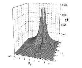
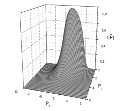
Figure 1: Momentum distribution of produced bosons (left)and fermions (right) at time $t=0.05$. The influence of the back reaction is not included.

When the BR mechanism is taken into account, the regular momentum dependence of the distribution function is destroyed (Figs. 2-5; the result like that in Fig. 3 was obtained previously in [2] but in the framework of different approach).

At the same time Fig. 4 and Fig. 5 demonstrate the existence of periodic temporal behavior of the distribution function. Two-dimensional representation in Fig. 5 clearly shows how a ’dog-brush’ structure of the distribution function along the $P_{3}$ axis is combined with the periodic time structure along the time axis.

     

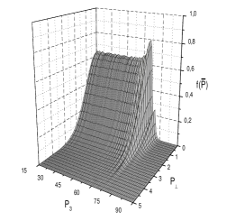
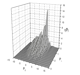
Figure 2: Momentum distributions of produced bosons without (left) and with inclusion (right) of the back reaction at time $t=10$.

     

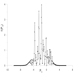
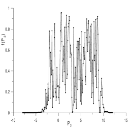
Figure 3: Momentum distributions of produced bosons (left) and fermions (right) at time $t=25$. Transversal momentum $P_{\perp}=0$ in both cases.

     

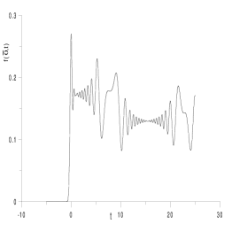
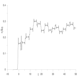
Figure 4: Time evolution of boson (left) and fermion (right) distribution function $f(\vec{0},t)$.

     

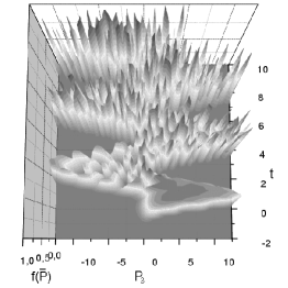
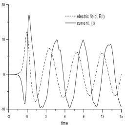
Figure 5: Time evolution of $f(0,P_{3},t)$ (left), electrical field and current (right) for the fermion case

4 Conclusion

Thus, the BR equations generate some large-scale structure on the background of small-scale multi-mode complex dynamics. The small-scale trembling is a manifestation of vacuum oscillations. Trembling frequency is increasing with time. The smoothed initial distribution function in Fig. 5 corresponds to the external field impulse. Large-scale wiggles in the distribution function is a consequence of self-organization of the system [15] due to the growth of the collective plasma oscillations.

The presented results provide some evidence that the inclusion of the BR mechanism into consideration of the pair creation gives rise to stochastic behavior of the system. It is not excluded that a dynamical chaos can be found also at other values of the parameter $eE$, however this needs additional numerical investigations. It is quite possible that the revealed stochastic features of the vacuum pair creation is a source of the statistical behavior observed in multiple particle production.

References

References

- [1] G. Gatoff, A. K. Kerman, and T. Matsui, Phys. Rev. D 36, 114 (1987).
- [2] Y. Kluger, J. M. Eisenberg, and B. Svetitsky, Int. J. Mod. Phys. E 2, 333 (1993).
- [3] Y. Kluger, E. Mottola, and J. M. Eisenberg, Phys. Rev. D 58, 125015 (1998).
- [4] N. D. Birrell and P. C. W. Davis, Quantum fields in curved space-time, (Cambridge University Press, Cambridge, 1982).
- [5] W. Greiner, B. Müller, and J. Rafelski, Quantum Electrodynamics of Strong Fields (Springer-Verlag, Berlin, 1985).
- [6] A. A. Grib, S. G. Mamaev, and V. M. Mostepanenko, Vacuum quantum effects in strong external fields, (Atomizdat, Moscow, 1988).
- [7] J. Rau and B. Muller, Phys. Rep. 272, 1 (1996).
- [8] S. A. Smolyansky et al, GSI-Preprint-97-92, Regensburg, 1997.
- [9] S. M. Schmidt et al, Int. J. Mod. Phys. E 7, 709 (1998).
- [10] S. M. Schmidt et al, Phys. Rev. D 59, 094005 (1999).
- [11] J. C. R. Bloch et al, Phys. Rev. D 60, 116011 (1999).
- [12] G. Baym, Phys. Lett. B 138, 18 (1984).
- [13] S. A. Smolyansky et al, work in progress.
- [14] S. G. Mamaev and N. N. Trunov, Sov. Journ. Nucl. Phys, 30, 1301 (1979).
- [15] H. Haken, Advanced Synergetics, Springer Series in Synergetics, v.20, (Springer-Verlag, Berlin, 1983).