(Field) Symmetrization Selection Rules

Abstract

QCD and QED exhibit an infinite set of three–point Green’s functions that contain only OZI rule violating contributions, and (for QCD) are subleading in the large $N_{c}$ expansion. The Green’s functions describe the “decay” of a $J^{PC}=\{1,3,5\ldots\}^{-+}$ exotic hybrid meson current to two $J=0$ (hybrid) meson currents with identical $P$ and $C$. We prove that the QCD amplitude for a neutral hybrid $\{1,3,5\ldots\}^{-+}$ exotic current to create $\eta\pi^{0}$ only comes from OZI rule violating contributions under certain conditions, and is subleading in $N_{c}$.

Keywords: symmetrization, selection rule, Green’s function, decay, $J^{PC}$ , hybrid

PACS number(s): 11.15.Pg   11.15.Tk    11.30.Na   11.55.-m    12.38.Aw    12.39.Mk    13.25.Jx

1 Introduction

More than a decade ago Lipkin argued that an explicitly identified contribution to the decay of a $J^{PC}=\{1,3,5\ldots\}^{-+}$ “exotic” hybrid meson to $\eta\pi$ vanishes [2]. Here $J$ denotes the internal angular momentum, $P$ (parity) the reflection through the origin and $C$ (charge conjugation) particle–antiparticle exchange. These are conserved quantum numbers of the strong and electromagnetic interactions. By “hybrid meson” we mean a fermion–antifermion with additional gauge bosons. “Exotic” means that the $J^{PC}$ cannot be constructed for conventional mesons in the quark model, or equivalently that there are no local currents built only from a fermion and antifermion field that can have these $J^{PC}$.

Lipkin’s intuitive argument was later extended and placed in a more formal context, called “symmetrization selection rules” [3]. However, these need to be converted into rigorous quantum field theoretic arguments, which is the subject of the current work.

We outline Lipkin’s intuitive argument for the decay of a positively charged $J^{P}=1^{-},\;3^{-},\;\ldots$ state to $\eta\pi^{+}$ when strong interactions with isospin symmetry is assumed. G-parity conservation implies that the neutral isospin partner of the initial state is $J^{PC}$ exotic. We consider the decay process where a quark and antiquark in the initial state proceed in such a way that the quark ends up in the one final meson, and the antiquark in the other meson (Fig. 1). This decay process is called “connected”, because each meson is connected to the other mesons via quark lines. The gluons are not indicated. The fact that the neutral isospin partner of the initial state is $J^{PC}$ exotic, and that the initial state contains a quark and antiquark, implies that the initial state is a hybrid meson. The argument is depicted in Fig. 1. Taking the initial hybrid at rest, the $\eta$ and $\pi^{+}$ emerge with momenta $-\bf k$ and $\bf k$ respectively. First consider the three top left diagrams. The top diagram has a negative sign in front by convention. When the transformation ${\bf k}\leftrightarrow-{\bf k}$ is applied, the middle diagram is obtained, noting that the decay is in an odd partial wave, which acquires a minus sign under the transformation. This is a general property of odd partial waves. The bottom diagram is obtained by noting that the amplitude to create a $u\bar{u}$ pair is the same as for a $d\bar{d}$ pair by the assumption of isospin symmetry, which treats the up and down quarks the same. The three top right “hadronic” diagrams are now obtained from the three top left “quark” diagrams by attaching the initial hybrid to the initial $u\bar{d}$ quarks, and the final $\pi^{+}$ to the final $u\bar{d}$ quarks. Since the flavour wave function of the $\eta$ is proportional to $u\bar{u}+d\bar{d}$, it is attached to either $u\bar{u}$ or $d\bar{d}$, with a positive relative sign. Because each of the three top left quark diagrams are equal, it follows that each of the three top right hadronic diagrams are equal. The two bottom diagrams depict the decay amplitude, taking into account that there are two possible ways for the final $\eta$ and $\pi^{+}$ to couple, since the quark in the initial state can go either to the $\eta$ or the $\pi$. Looking back at the top right hadronic diagrams one immediately notices that the decay amplitude vanishes. This is the desired result.

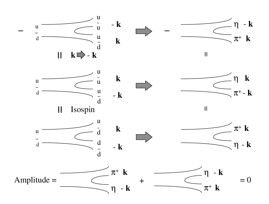
Figure 1: Lipkin’s intuitive argument.

The argument above can be repeated without assuming isospin symmetry, as will be the case in the remainder of this work, if the initial state is neutral. Hence isospin is not an essential assumption. It appears strange that a decay amplitude vanishes from very general considerations if the decay is allowed by the conserved quantum numbers of the strong interaction. This paradox is resolved when one notices that it was only argued that the connected contribution to the decay vanishes, not the entire decay amplitude. Lipkin’s argument serves as a guide to how a quantum field theoretic argument would proceed.

In this Paper we demonstrate that some explicitly identified contributions to certain three–point Green’s functions vanish. This is called field symmetrization selection rules. Particularly, the connected (Okubo–Zweig–Iizuka (OZI) allowed) contribution to each Green’s function vanishes. Hence, the Green’s function only has a disconnected (OZI forbidden) contribution, which is expected to be phenomenologically suppressed by virtue of the OZI rule [4]. The Green’s function is built from two $J=0$ (hybrid) meson currents with identical $P$ and $C$, and a $J^{PC}=\{1,3,5\ldots\}^{-+}$ exotic hybrid meson current.

We subsequently investigate the physical consequences. The amplitude for a $\{1,3,5\ldots\}^{-+}$ hybrid current to create $\eta\pi^{0}$ is shown to be proportional to the Green’s function under certain conditions. Because some explicitly identified contributions to the Green’s function vanish, it follows that the amplitude does not come from these contributions, called symmetrization selection rules at the hadronic level. Particularly, the amplitude does not arise from the connected contribution to the Green’s function, and hence only from the disconnected contribution, which is expected to be suppressed by virtue of the OZI rule. The experimental consequences pertain to a central issue in hadron spectroscopy: the search for hybrid meson bound states beyond conventional mesons and baryons.

For Quantum Chromodynamics (QCD) with a large number of colours $N_{c}$, the foregoing conclusions will be expressed as follows. Because a disconnected contribution to a Green’s function is subleading in the large $N_{c}$ expansion, and the Green’s function only has a disconnected contribution, the Green’s function is subleading in $N_{c}$. Also, since the amplitude for a $\{1,3,5\ldots\}^{-+}$ hybrid current to create $\eta\pi^{0}$ only comes from the disconnected contribution to the Green’s function, it is subleading in $N_{c}$.

It has previously been shown that the connected part of the quenched Euclidean three–point Green’s function of specific hybrid meson neutral $1^{-+}$ and two pseudoscalar ($J=0$) currents vanishes exactly in QCD, if isospin symmetry is assumed [5]. We remove the three italized superfluous assumptions, but still need the connected part and hybrid meson currents. We also generalize beyond specific currents, beyond $1^{-+}$ and pseudoscalar currents, beyond the connected part, and beyond QCD.

In section 2 the currents and Green’s functions are introduced. The principle of symmetrization is developed. In section 3 the Green’s functions are calculated leading to succinctly stated field symmetrization selection rules. An explicit example is discussed. In section 4 the physical consequences are investigated, yielding symmetrization selection rules at the hadronic level, which are concisely stated. Section 5 studies the selection rules in the large $N_{c}$ expansion. Section 6 contains further remarks.

2 Symmetrization

Consider local currents of the form

$$\{A_{\mu}(x),B(x),C(x)\}=\sum_{i}\bar{\psi}_{i}(x)\;\{a_{i}a_{\mu}(x),b_{i}b(x),c_{i}c(x)\}\;{\psi}_{i}(x)$$ (1)

where ${\psi}_{i}(x)$ is a quark or lepton field of flavour $i$, and $a_{i},b_{i},c_{i}$ are c–numbers weighting the flavours. The currents are diagonal in flavour. The “matrices” $a_{\mu}(x),\;b(x)$ and $c(x)$ contain an arbitrary number of Dirac matrices, Gell–Mann colour matrices, derivatives (acting both to the left and the right), gluon or photon fields and correspond to gauge invariant currents [6]. A common choice for the flavour structure of the three currents is $\bar{u}u-\bar{d}d,\;\bar{u}u+\bar{d}d-\bar{s}s$ and $\bar{u}u-\bar{d}d$, interpolating for an isovector resonance, an $\eta$ and a $\pi^{0}$. The matrix $a_{\mu}(x)$ in Eq. 1 is chosen to ensure that $P=-$. We require that currents $B$ and $C$ have $J=0$, as well as equality of $b(x)$ and $c(x)$, implying equal $P$ and $C$. Note that equality of the matrices $b(x)$ and $c(x)$ does not imply equality of the currents $B(x)$ and $C(x)$. Because $C$ is the same for both these currents, charge conjugation conservation requires that the $C$ of $A_{\mu}(z)$ is $+$. Take $A_{\mu}$ to have odd $J$ [7]. Hence $A_{\mu}$ must be chosen to have $J^{PC}=\{1,3,5\ldots\}^{-+}$. These are exotic quantum numbers, and $A_{\mu}$ is built from a fermion and an antifermion field, so that the current is a hybrid current, i.e. has to contain at least one gluon or photon field. For the current with $J\neq 0$, the appropriate Lorentz indices are indicated by $\mu$.

We start by demonstrating that certain three–point Green’s functions are equal to their antisymmetric parts. This is done by first defining the spatial Green’s function, $G_{\mu}(x,y,z)$, and decomposing it into symmetric and antisymmetric parts. The Green’s function of interest will be the Fourier transform of the spatial Green’s function, $G_{\mu}({\bf p},t)$. We then argue that the Fourier transform of the symmetric part of the spatial Green’s function, $G_{\mu}^{S}({\bf p},t)$, vanishes. Hence, $G_{\mu}({\bf p},t)$ equals the Fourier transform of the antisymmetric part of the spatial Green’s function, $G_{\mu}^{A}({\bf p},t)$.

Define the three–point Minkowski space Green’s function

$$G_{\mu}(x,y,z)=\langle 0|\;B(x)\;C(y)\;A_{\mu}(z)\;|0\rangle$$ (2)

with $x_{0}=y_{0}\equiv t,\;z_{0}=0$ and ${\bf z}={\bf 0}$. The Green’s function describes the decay (production) process of a current $A_{\mu}(z)$ at time 0 propagating into the final (initial) currents $B(x)$ and $C(y)$ at some positive (negative) time $t$. Although we shall refer to $G_{\mu}(x,y,z)$ as a “Green’s function”, the usual usage of the term requires the currents to be at different times, i.e. $x_{0}\neq y_{0}$, with the currents ordered from positive to negative times. The Green’s function $G_{\mu}(x,y,z)$ can be written as $G_{\mu}^{S}(x,y,z)+G_{\mu}^{A}(x,y,z)$, i.e. the sum of parts symmetric and antisymmetric under exchange of $x$ and $y$, as any function of $x$ and $y$ can be written.

Define the Fourier transforms

$${G_{\mu}}({\bf p},t) \equiv \int\;d^{3}x\;d^{3}y\;e^{i({\bf p}\cdot{\bf x}-{\bf p}\cdot{\bf y})}\;{G_{\mu}}(x,y,z)$$ (3)

$$\left\{G_{\mu}^{S}({\bf p},t),\;G_{\mu}^{A}({\bf p},t)\right\} \equiv \int\;d^{3}x\;d^{3}y\;e^{i({\bf p}\cdot{\bf x}-{\bf p}\cdot{\bf y})}\;\left\{G_{\mu}^{S}(x,y,z),\;G_{\mu}^{A}(x,y,z)\right\}$$ (4)

Note that these Fourier transforms cannot be inverted to give the spatial Green’s functions, since they only have one momentum variable ${\bf p}$. From Eqs. 3 and 4 it follows that $G_{\mu}({\bf p},t)=G_{\mu}^{S}({\bf p},t)+G_{\mu}^{A}({\bf p},t)$.

By exchanging integration variables ${\bf x}\leftrightarrow{\bf y}$

$$G_{\mu}(-{\bf p},t)=\int\;d^{3}x\;d^{3}y\;e^{i({\bf p}\cdot{\bf x}-{\bf p}\cdot{\bf y})}\;{G_{\mu}}(({\bf y},t),({\bf x},t),z)$$

$$=\int\;d^{3}x\;d^{3}y\;e^{i({\bf p}\cdot{\bf x}-{\bf p}\cdot{\bf y})}\;\left\{G_{\mu}^{S}(y,x,z)+G_{\mu}^{A}(y,x,z)\right\}=G_{\mu}^{S}({\bf p},t)-G_{\mu}^{A}({\bf p},t)$$ (5)

Exchanging integration variables ${\bf x}\rightarrow-{\bf x}$ and ${\bf y}\rightarrow-{\bf y}$ yields

$$G_{\mu}(-{\bf p},t)=-G_{\mu}({\bf p},t)$$ (6)

by using that ${G_{\mu}}((-{\bf x},t),(-{\bf y},t),z)=-{G_{\mu}}(x,y,z)$, by conservation of parity. We henceforth restrict ourselves to the parity conserving theories of Quantum Electrodynamics (QED) and QCD. We also used that the product of the parities of the currents $B(x)$, $C(y)$ and $A_{\mu}(z)$ is $-1$, which follows from the assumptions below Eq. 1. This means that the decay (production) process is in odd partial wave. Eq. 6 is a well–known property of such a process.

Combining Eqs. 2 and 6 yields the result

$$G^{S}_{\mu}({\bf p},t)=0$$ (7)

Bose symmetry states that identical bosons are not allowed in an odd partial wave. The way one shows this would be analogous to the steps above if $G^{A}_{\mu}({\bf p},t)=0$. Hence, the Fourier transform of the symmetric part of $G_{\mu}(x,y,z)$ in Eq. 7 vanishes by arguments that are the field theoretical version of Bose symmetry.

From Eq. 7 follows the desired result

$$G_{\mu}({\bf p},t)=G^{A}_{\mu}({\bf p},t)$$ (8)

3 Field Symmetrization Selection Rules

We proceed to explicitly identify some contributions to $G_{\mu}({\bf p},t)$ that vanish. This is attained via partially evaluating $G_{\mu}^{A}({\bf p},t)$. It is subsequently shown that the action of a certain operator, $\hat{O}_{{\bf p}}$, on the Fourier transform of the antisymmetric part of the Green’s function, $\hat{O}_{{\bf p}}\;G_{\mu}^{A}({\bf p},t)$, does not contain some contributions. Because $G_{\mu}^{A}({\bf p},t)=G_{\mu}({\bf p},t)$ from Eq. 8, it follows that $\hat{O}_{{\bf p}}\;G_{\mu}({\bf p},t)$ does not contain these contributions.

We now evaluate the contributions to the Green’s function $G_{\mu}^{A}(x,y,z)$ with the currents in Eq. 1, using that $G_{\mu}^{A}(x,y,z)=\frac{1}{2}\;(G_{\mu}(x,y,z)-G_{\mu}(y,x,z))$,

$$G_{\mu}^{A}(x,y,z) = \frac{1}{2}\;\langle 0|\;\left(\;B(x)\;C(y)-B(y)\;C(x)\;\right)\;A_{\mu}(z)\;|0\rangle$$ (9)

$$= \frac{1}{2}\;\sum_{i\;j}b_{i}c_{j}\;\langle 0|\;\left(\;\bar{\psi}_{i}(x)\;b(x)\;{\psi}_{i}(x)\;\;\bar{\psi}_{j}(y)\;c(y)\;{\psi}_{j}(y)\;-\right.$$

$$\hskip 79.6678pt\left.\bar{\psi}_{i}(y)\;b(y)\;{\psi}_{i}(y)\;\;\bar{\psi}_{j}(x)\;c(x)\;{\psi}_{j}(x)\;\right)\;A_{\mu}(z)\;|0\rangle$$

The various contributions to this expression are now discussed. Consider contributions to the expression where the same flavours are isolated in the currents $B(x)$ and $C(y)$, i.e. contributions where $i=j$. Using Eqs. 4 and 9, these contributions to $G_{\mu}^{A}({\bf p},t)$ can be written

$$G_{\mu}^{A}({\bf p},t)\sim\int\;d^{3}x\;d^{3}y\;e^{i({\bf p}\cdot{\bf x}-{\bf p}\cdot{\bf y})}\;\frac{1}{2}\;\sum_{i}b_{i}c_{i}\;$$

$$\mbox{}\times\langle 0|\;\left[\;\bar{\psi}_{i}(x)\;b(x)\;{\psi}_{i}(x)\;,\;\bar{\psi}_{i}(y)\;b(y)\;{\psi}_{i}(y)\;\right]\;A_{\mu}(z)\;|0\rangle\equiv\Lambda_{\mu}({\bf p},t)$$ (10)

where we used $b(x)=c(x)$, and denoted the contributions by $\Lambda_{\mu}$. The important observation is that the difference of currents in Eq. 9 has simplified to the commutator of currents in Eq. 3. It is possible to show that $\Lambda_{\mu}$ has a polynomial dependence on ${\bf p}$ (see Appendix) [8]. There hence exists a polynomial operator (containing a derivative of high enough power in ${\bf p}$) with the property that $\hat{O}_{{\bf p}}\;\Lambda_{\mu}({\bf p},t)=0$. This result will later be demonstated in an explicit example. We conclude from Eq. 3 that $\hat{O}_{{\bf p}}\;G_{\mu}^{A}({\bf p},t)$, and from Eq. 8 also $\hat{O}_{{\bf p}}\;G_{\mu}({\bf p},t)$, do not contain contributions from the same flavour in currents $B(x)$ and $C(y)$, a result which corrects the former treatment [9]. Although this is the desired result, and the end of the mathematical derivation, it will be pivotal to develop a more intuitive understanding of the contributions.

$\hat{O}_{{\bf p}}\;G_{\mu}({\bf p},t)$ is an operator acting on the Fourier transform of $G_{\mu}(x,y,z)$. For the purpose of illustration in the next few paragraphs, consider the time $t$ to be positive, with $B(x)$ slightly advanced at time $x_{0}=t+\delta t$ with respect to $C(y)$ at time $y_{0}=t$ in the definition of $G_{\mu}(x,y,z)$ in Eq. 2. Here $\delta t$ is small, positive and non-zero. The sign of $t$ or the magnitude of $\delta t$ will not change our eventual conclusions. Since all the currents are at different times, with the currents ordered from large to small times, it follows that $G_{\mu}(x,y,z)$ is a Green’s function according to the usual usage of the term, which implies that it can be represented by a path integral. For concreteness, consider the contribution to $G_{\mu}(x,y,z)$ in Eq. 2 from the up quark flavours in the currents $B(x)$, $C(y)$ and $A_{\mu}(z)$ in Eq. 1, which is (modulo $a_{u}b_{u}c_{u}$)

$$\int{\cal D}A\;{\cal D}\bar{\psi}\;{\cal D}\psi\;\delta(f(A))\;\mbox{det}{\cal M}_{F}\;\bar{u}(x)b(x)u(x)\;\bar{u}(y)c(y)u(y)\;\bar{u}(z)a_{\mu}(z)u(z)\;\exp(-i\int d^{4}x\;{\cal L})$$ (11)

$$=\int\;{\cal D}A\;\delta(f(A))\;\mbox{det}{\cal M}_{F}\;\mbox{det}\gamma_{0}S^{-1}\;\exp(-i\int d^{4}x\;{\cal L}^{(A)})\;$$

$$\{{\mbox{Tr}}[-a_{\mu}(z)\;S_{u}^{A}(z,x)\;b(x)\;S_{u}^{A}(x,y)\;c(y)\;S_{u}^{A}(y,z)-a_{\mu}(z)\;S_{u}^{A}(z,y)\;c(y)\;S_{u}^{A}(y,x)\;b(x)\;S_{u}^{A}(x,z)]$$

$$+\;{\mbox{Tr}}[a_{\mu}(z)\;S_{u}^{A}(z,x)\;b(x)\;S_{u}^{A}(x,z)]\;{\mbox{Tr}}[c(y)\;S_{u}^{A}(y,y)]\;+\;{\mbox{Tr}}[a_{\mu}(z)\;S_{u}^{A}(z,y)\;c(y)\;S_{u}^{A}(y,z)]\;$$

$$\mbox{}\times\;{\mbox{Tr}}[b(x)\;S_{u}^{A}(x,x)]\;+\;{\mbox{Tr}}[a_{\mu}(z)\;S_{u}^{A}(z,z)]\;{\mbox{Tr}}[b(x)\;S_{u}^{A}(x,y)\;c(y)\;S_{u}^{A}(y,x)]$$

$$-\;{\mbox{Tr}}[a_{\mu}(z)\;S_{u}^{A}(z,z)]\;{\mbox{Tr}}[b(x)\;S_{u}^{A}(x,x)]\;{\mbox{Tr}}[c(y)\;S_{u}^{A}(y,y)]\}$$

The gauge–fixing condition $\delta(f(A))$ and Faddeev–Popov determinant $\mbox{det}{\cal M}_{F}$ are indicated. The QCD / QED Lagrangian is denoted by ${\cal L}$ and the part containing terms without fermions ${\cal L}^{(A)}$. The up quark propagator in a background field is $S_{u}^{A}(x,y)$ and the fermion determinant (containing fermion loops) $\mbox{det}\gamma_{0}S^{-1}$ [10].

Figure 2: Topologies contributing to Eq. 11.

The terms on the right hand side (R.H.S.) of Eq. 11 correspond to the topologies in Fig. 2. This is seen by associating with each up quark propagator an up quark line in the figure. Also, $z$ is associated with the left hand side (L.H.S.) of each topology, and $x,\;y$ with the blobs on the R.H.S. In Eq. 11 the first two terms correspond to the quark line “connected” topology 1 in Fig. 2, the second two to topology 2, term five to topology 3b and term six to topology 3a.

The topologies hence represent all the different ways that a fermion and antifermion field on the L.H.S. of Eq. 11 can be “contracted” by the fermion integration to yield the fermion propagators on the R.H.S.

Similar manipulations to Eq. 11 can be performed for contributions where not all the fermions in the currents are up quarks, or not all the fermions have the same flavour.

From Fig. 2 it can be seen that topologies 1 and 3b have the interesting property that when a certain flavour contributes from current $B(x)$, then the same flavour contributes from current $C(y)$. This is because the currents are diagonal in flavour. Although $B(x)$ and $C(y)$ contain various different flavour structures according to Eq. 1, topologies 1 and 3b force only the same fermion flavours in $B(x)$ and $C(y)$ to contract. For the other topologies, it is sometimes the case that the flavours from two currents are the same, but not always. Recalling that $\hat{O}_{{\bf p}}\;G_{\mu}({\bf p},t)$ does not contain contributions from the same flavour in currents $B(x)$ and $C(y)$, we derive

Field symmetrization selection rules (FSSR): All contributions to the three–point Green’s function $\hat{O}_{{\bf p}}\;G_{\mu}({\bf p},t)$ from the connected topology 1 and topology 3b (and some from topologies 2 and 3a), i.e. contributions from the same flavour in currents $B(x)$ and $C(y)$, vanish exactly for all momenta ${\bf p}$ and times $t$ for an infinite set of equal matrices $b(x)=c(x)$ and different flavour structure currents $B(x)$ and $C(y)$ in QCD and QED. The Green’s function decribes the “decay” of a $J^{PC}=\{1,3,5,\ldots\}^{-+}$ exotic hybrid meson current to two $J=0$ (hybrid) meson currents $B(x)$ and $C(y)$, which are identical $(b(x)=c(x))$, e.g. have identical parity and charge conjugation, except possibly for their flavour.

The contributions that vanish by the FSSR are those from the same flavour in currents $B(x)$ and $C(y)$. Since the product $B(x)\;C(y)$ occurs in the Green’s function (see Eq. 2), these are contributions of the form $b_{i}c_{i}\;\bar{\psi}_{i}(x)\;b(x)\;{\psi}_{i}(x)\;\bar{\psi}_{i}(y)\;c(y)\;{\psi}_{i}(y)$, where $i$ indicates the flavour, and no summation is implied. It is evident that the precise values of $b_{i}$ and $c_{i}$, i.e. the flavour structure of $B(x)$ and $C(y)$, do not affect the fact that the contributions vanish by the FSSR. The same is true for $A_{\mu}(z)$. For example, both the common choice of $\bar{u}u-\bar{d}d,\;\bar{u}u+\bar{d}d-\bar{s}s$ and $\bar{u}u-\bar{d}d$ for the flavour structure of $A_{\mu}(z)$, $B(x)$ and $C(y)$, and the alternative choice of respectively $\bar{u}u-2\bar{d}d,\;\bar{u}u+\bar{d}d-2\bar{s}s$ and $2\bar{u}u-\bar{d}d$, obey the FSSR.

The FSSR do not depend on the various parameters of QCD and QED, i.e. masses, couplings, charges, number of colours and flavours, but do require the $CP$ violating $\theta$ parameter to be zero, since this parameter violates parity conservation. FSSR also occur is pure QED, where QCD interactions are turned off.

We now discuss an example to which the FSSR apply. The gauge invariant isovector–like local current $A_{\mu}(z)=(T^{i}_{jk})_{\mu}\;\left(\bar{u}(z)F^{a}_{jk}(z)\lambda^{a}\gamma_{i}u(z)-\bar{d}(z)F^{a}_{jk}(z)\lambda^{a}\gamma_{i}d(z)\right)$ is $J^{PC}=1^{-+}$ exotic [5], where $\gamma_{i}$ and $\lambda^{a}$ are Dirac and Gell–Mann colour matrices respectively, and $(T^{i}_{jk})_{\mu}$ is a tensor combining the spatial indices $i,j,k$ to build a spin 1 object. It is a hybrid current, since it contains a gluon field, as can be seen by the presence of the gluon field tensor $F^{a}_{jk}$. The gauge–invariant isoscalar– and isovector–like local currents $B(x)=\bar{u}(x)\gamma_{5}u(x)+\bar{d}(x)\gamma_{5}d(x)-\bar{s}(x)\gamma_{5}s(x)$ and $C(y)=\bar{u}(y)\gamma_{5}u(y)-\bar{d}(y)\gamma_{5}d(y)$ are pseudoscalar ($J^{PC}=0^{-+}$), with $\gamma_{5}$ a Dirac matrix. Note that $b(x)=c(x)=\gamma_{5}$, but that $B(x)\neq C(x)$. Also, we do not assume isospin symmetry. To evaluate $\Lambda_{\mu}$ in Eq. 3, the commutator $[\bar{u}(x)\gamma_{5}u(x),\bar{u}(y)\gamma_{5}u(y)]$ must be evaluated. The commutator can be shown to equal $\delta^{3}({\bf x}-{\bf y})\;\left(\>\bar{u}(x)\gamma_{5}\gamma_{0}\gamma_{5}u(y)-\bar{u}(y)\gamma_{5}\gamma_{0}\gamma_{5}u(x)\>\right)$. Because of the delta function, it is immediate that $\Lambda_{\mu}({\bf p},t)$ in Eq. 3 is independent of ${\bf p}$, i.e. it has a polynomial dependence on ${\bf p}$. The polynomial operator $\hat{O}_{{\bf p}}=\frac{\partial}{\partial{\bf p}}$ has the promised property that $\hat{O}_{{\bf p}}\;\Lambda_{\mu}({\bf p},t)=0$. In this example, the commutator actually vanishes because the delta function forces $x=y$, so that $\delta^{3}({\bf x}-{\bf y})\;\left(\>\bar{u}(x)\gamma_{5}\gamma_{0}\gamma_{5}u(y)-\bar{u}(y)\gamma_{5}\gamma_{0}\gamma_{5}u(x)\>\right)=0$; implying that $\Lambda_{\mu}=0$, and one can take $\hat{O}_{{\bf p}}=1$. There does, however, exist examples where $\hat{O}_{{\bf p}}$ is not trivial as in this case. For example, one can show that replacing $b(x)=\gamma_{5}$ by $b(x)=\gamma_{5}F^{a}_{\mu\nu}(x)\;F^{a\;\mu\nu}(x)$ yields a non–trivial $\hat{O}_{{\bf p}}$.

4 Symmetrization Selection Rules at the Hadronic Level

We now investigate the physical consequences of the FSSR, particularly the amplitude for a $\{1,3,5\ldots\}^{-+}$ hybrid current to create $\eta\pi^{0}$, which can be obtained from the Green’s function. This is done via an alternative route to the former treatment [5], which contains erroneous aspects [11].

A natural quantity to obtain from the three–point Green’s function is the amplitude for the hybrid current to create a stable two–body state. The hybrid current is not expected to interpolate for a stable particle, so that we shall not be able to extract the T–matrix for a stable hybrid particle to decay to the two–body state. To obtain the amplitude, a complete set of asymptotic, i.e. stable, states $n$ are inserted in the Green’s function. The leads to a general relation (Eq. 4) between the Green’s function and the amplitudes for a $\{1,3,5\ldots\}^{-+}$ hybrid current to create the asymptotic states. Under certain conditions this equation can be simplified to show that the Green’s function is proportional to the amplitude for a $\{1,3,5\ldots\}^{-+}$ hybrid current to create $\eta\pi^{0}$, Eq. 15. Because some explicitly identified contributions to $\hat{O}_{{\bf p}}\;G_{\mu}({\bf p},t)$ vanish, it follows that the amplitude does not come from these contributions.

Restricting to QCD on its own [12], from the definition Eq. 3

$${G_{\mu}}({\bf p},t)=\int\;d^{3}x\;d^{3}y\;e^{i({\bf p}\cdot{\bf x}-{\bf p}\cdot{\bf y})}\sum_{n}\;\langle 0|{B}({\bf x},0)\;{C}({\bf y},0)\;e^{-iHt}|n\rangle\;\langle n|{A_{\mu}}(z)|0\rangle$$ (12)

where we used time translational invariance of the fields $B(x)$ and $C(y)$, e.g. $B({\bf x},t)=e^{iHt}B({\bf x},0)e^{-iHt}$, with $H$ the QCD Hamiltonian. The product ${B}({\bf x},0)\;{C}({\bf y},0)$ and ${A_{\mu}}(z)$ should be colourless to make the expression non–zero, which is the case since each current has been assumed to be gauge invariant. If the quarks have their physical masses, the lowest asymptotic states contain the states $\pi$ and $\eta$, the lowest stable states of the QCD spectrum [13]. The $\pi$ only decays weakly and electromagnetically, and is hence stable as far as QCD on its own is concerned. The $\eta$ has a width of only $10^{-5}$ times the typical hadronic width of $100$ MeV, so that it is very nearly stable.

Space translational invariance of the fields $B(x)$ and $C(y)$, e.g. $B({\bf x},0)=e^{-i{\bf P}\cdot{\bf x}}B(0)e^{i{\bf P}\cdot{\bf x}}$, with ${\bf P}$ the QCD momentum operator, is now employed. Performing one of the integrations in Eq. 12 (the one over ${\bf x}+{\bf y}$)

$${G_{\mu}}({\bf p},t)=\sum_{n}\;(2\pi)^{3}\;\delta^{3}({\bf p}_{n})\;e^{-iE_{n}t}\;\langle 0|{(}\int d^{3}x\;e^{i{\bf p}\cdot{\bf x}}\;{B}({\bf x},0){)}\;{C}(0)|n\rangle\;\langle n|{A_{\mu}}(z)|0\rangle$$ (13)

where the integration variable ${\bf x}-{\bf y}$ is denoted by ${\bf x}$. Here ${\bf p}_{n}$ and $E_{n}$ are the momentum and energy of state $n$. The Euclidean space analogue of all the steps up to here is obtained by taking $t\rightarrow-it$. However, we now restrict to Minkowski space in order to integrate over time. From Eq. 13

$$\int^{\infty}_{-\infty}dt\;\hat{O}_{{\bf p}}\;G_{\mu}({\bf p},t)\;e^{iEt}$$

$$=\sum_{n}\;(2\pi)^{4}\;\delta^{3}({\bf p}_{n})\;\delta(E_{n}-E)\;\hat{O}_{{\bf p}}\;\langle 0|{(}\int d^{3}x\;e^{i{\bf p}\cdot{\bf x}}\;{B}({\bf x},0){)}\;{C}(0)|n\rangle\;\langle n|{A_{\mu}}(z)|0\rangle$$ (14)

where $E$ is a real number. The delta functions indicate that the asymptotic states are at rest and have energy $E$.

For $E$ below the $\pi^{+}\pi^{-}\pi^{0}$ or $\pi^{0}\pi^{0}\pi^{0}$ (called the $\pi\pi\pi$) threshold only $\pi\pi$ asymptotic states contribute. Since for two–pion states at rest $\langle\pi^{0}{\bf k}\;\pi^{0}-{\bf k}|{A_{\mu}}(z)|0\rangle$ and $\langle\pi^{+}{\bf k}\;\pi^{-}-{\bf k}|{A_{\mu}}(z)|0\rangle$ respectively vanish by Bose symmetry and $CP$ conservation, this forces the L.H.S. of Eq. 4 to be zero. If $E$ is above the $\pi\pi\pi$ threshold the sum in Eq. 4 can be shown to be infinite. However, we shall show below that if the $\eta\pi^{0}$ threshold can be made below the $\pi\pi\pi$ threshold, in contrast to experiment, the sum has only one contribution. This is important because we want a single amplitude on the R.H.S. of Eq. 4 to be proportional to the L.H.S.

In QCD we are free to tune the quark masses away from the masses corresponding to experiment. Taking the $\eta\pi^{0}$ threshold to be below the $\pi\pi\pi$ threshold for some range of quark masses, is called the “QCD dynamics” condition. This condition can heuristically be satisfied by noting that four times higher up / down quark masses would yield a two times heavier $\pi$, while the $\eta$ mass would not change much, so that $\eta$ can move below the $\pi\pi$ threshold. This follows from the fact that the $\pi$ and $\eta$ masses, $m_{\pi}$ and $m_{\eta}$, are $c\sqrt{m_{u}+m_{d}}$ and $c\sqrt{(4m_{s}+m_{u}+m_{d})/3}$ by chiral symmetry breaking, with $m_{u,d,s}$ the current quark masses and $c$ a constant. Under the QCD dynamics condition $\eta$ lies below $\pi\pi$ threshold, so that it is stable. This means that the formalism is exact when asymptotic states involving $\eta$ are inserted in Eq. 12.

Consider $E$ between the $\eta\pi^{0}$ and $\pi\pi\pi$ thresholds. Then the sum in Eq. 4 is over all on–shell $\pi$ and $\eta$ states with momenta ${\bf k}_{1}$ and ${\bf k}_{2}$ respectively, i.e. $\sum_{n}=\int d^{3}k_{1}\;/(2\pi)^{3}\;\int d^{3}k_{2}\;/(2\pi)^{3}$. Noting that ${\bf p}_{n}={\bf k}_{1}+{\bf k}_{2}$ and $E_{n}=\sqrt{{\bf k}_{1}^{2}+m_{\pi}^{2}}+\sqrt{{\bf k}_{2}^{2}+m_{\eta}^{2}}$, and performing the integrations, Eq. 4 implies that

$$\int^{\infty}_{-\infty}dt\;\hat{O}_{{\bf p}}\;G_{m}({\bf p},t)\;e^{iEt}=f(q^{2})\;\frac{1}{8(2\pi)^{2}E^{4}}\;\sqrt{(E^{2}-(m_{\pi}+m_{\eta})^{2})(E^{2}-(m_{\pi}-m_{\eta})^{2})}\;$$ (15)

$$\mbox{}\times(E^{4}-(m_{\pi}+m_{\eta})^{2}(m_{\pi}-m_{\eta})^{2})\int d\Omega_{{\bf k}}\;q_{m}\;\hat{O}_{{\bf p}}\;\langle 0|{(}\int d^{3}x\;e^{i{\bf p}\cdot{\bf x}}\;{B}({\bf x},0){)}\;{C}(0)|\pi{\bf k}\;\eta-{\bf k}\rangle$$

Here $q^{\mu}\equiv k_{1}^{\mu}-k_{2}^{\mu}$ and ${\bf k}_{1}=-{\bf k}_{2}\equiv{\bf k}$. In the expression $q^{2}$ is a function of $|{\bf k}|$, and $|{\bf k}|$ is restricted by $E_{n}=E$, so that $q^{2}$ is a function of $E$. The amplitude for a hybrid current to create $\eta$ and $\pi$ mesons, $\langle\pi{\bf k}\;\eta-{\bf k}|{A_{\mu}}(z)|0\rangle$, should occur in Eq. 15. However, we used the Lorentz properties of $\langle\pi{\bf k}\;\eta-{\bf k}|{A_{m}}(z)|0\rangle$ to define it as $q_{m}f(q^{2})$, with $m$ a spatial index, for $A_{\mu}$ having $J=1$ [14]. For a time index $m$ and other $J$ similar results follow.

On the R.H.S. of Eq. 15, $\langle 0|{B}({\bf x},0)\;{C}(0)|\pi{\bf k}\;\eta-{\bf k}\rangle$ is a property of $\eta$ and $\pi$. For example, it contains a term proportional to $\langle 0|{B}(0)|\pi{\bf k}\rangle\;\langle 0|{C}(0)|\eta{\bf k}\rangle$, a product of individual properties of $\pi$ and $\eta$, when the currents $B(0)$ ($C(0)$) have the same quantum numbers as the asymptotic states $\pi$ ($\eta$). One hence interprets Eq. 15 as meaning that the decay described by the three–point Green’s function on the L.H.S., is proportional to the decay amplitude described by $f(q^{2})$ on the R.H.S., up to a “constant” of proportionality which describes properties of $\eta$ and $\pi$. Suppression of the decay on the L.H.S. should hence translate into suppression of the decay on the R.H.S., since the properties of $\eta$ and $\pi$ should remain unaltered.

From Eq. 15, noting that $f(q^{2})$ is proportional to the L.H.S.,

Symmetrization selection rules at the hadronic level (SSR): The amplitude for a neutral $J^{PC}=\{1,3,5\ldots\}^{-+}$ exotic hybrid meson current to create or annihilate $\eta\pi^{0}$, $q_{m}f(q^{2})$, does not arise, in QCD, from contributions to $\hat{O}_{{\bf p}}\;G_{m}({\bf p},t)$ that vanish by the FSSR. This holds for quark masses chosen such that the $\eta\pi^{0}$ threshold is below the $\pi^{+}\pi^{-}\pi^{0}$ or $\pi^{0}\pi^{0}\pi^{0}$ thresholds, and for $E$ between these thresholds.

This concludes the physical consequences of the FSSR.

5 Large $N_{c}$

We now study the effect of taking $N_{c}$ to be large in QCD [15]. Here one makes a classification based on power counting in $N_{c}$. The amplitude $\langle\pi{\bf k}\;\eta-{\bf k}|{A_{\mu}}(z)|0\rangle$ is ${\cal O}(1)$ [16], so that $f(q^{2})$ is ${\cal O}(1)$. The contributions to the Green’s function from topology 1 is ${\cal O}(N_{c})$ to leading order, from topologies 2 and 3b ${\cal O}(1)$ and from topology 3a ${\cal O}(\frac{1}{N_{c}})$ [16], so that the L.H.S. of Eq. 15 would ordinarily be ${\cal O}(N_{c})$. However, since topology 1 does not contribute by the FSSR, the L.H.S. is ${\cal O}(1)$, and hence $f(q^{2})$ is ${\cal O}(\frac{1}{N_{c}})$ [17]. Hence both quantities are subleading to their usual $N_{c}$ counting. Whence

$$\frac{1}{N_{c}}\;\hat{O}_{{\bf p}}\;G_{\mu}({\bf p},t)\rightarrow 0\hskip 42.67912ptf(q^{2})\rightarrow 0\hskip 42.67912pt\mbox{as }N_{c}\rightarrow\infty$$ (16)

where both expressions ordinarily remain non–zero as $N_{c}\rightarrow\infty$. The two exactly vanishing expressions are respectively the consequences of the FSSR and SSR in large $N_{c}$. The SSR in large $N_{c}$ is: The hybrid $J^{PC}=\{1,3,5\ldots\}^{-+}\rightarrow\eta\pi^{0}$ amplitude is ${\cal O}(\frac{1}{N_{c}})$ in QCD, i.e. vanishes exactly in the large $N_{c}$ limit, for quark masses chosen such that the $\eta\pi^{0}$ threshold is below the $\pi^{+}\pi^{-}\pi^{0}$ or $\pi^{0}\pi^{0}\pi^{0}$ thresholds, and for $E$ between these thresholds. This is not the same as Bose symmetry, since $\eta$ and $\pi^{0}$ are not identical particles in the large $N_{c}$ limit. The finding that the amplitude for the hybrid current to decay to $\eta\pi^{0}$ is subleading in $N_{c}$ intuitively follows from the fact that OZI–violating processes are large $N_{c}$ suppressed.

The preceding discussion in this section assumed that the L.H.S. of Eq. 15 is “ordinarily” of ${\cal O}(N_{c})$. This is attained when $\langle 0|{B}({\bf x},0)\;{C}(0)|\pi{\bf k}\;\eta-{\bf k}\rangle$ on the R.H.S. of Eq. 15 is ${\cal O}(N_{c})$. This is true when the currents $B(x)$ ($C(y)$) individually have the same quantum numbers as the asymptotic states $\pi$ ($\eta$) or $\eta$ ($\pi$) [16], i.e. when the currents are pseudoscalar. Up to this point in the Paper we have not required either of the currents to have a specific parity and charge conjugation. However, if the currents are not pseudoscalar, $\langle 0|{B}({\bf x},0)\;{C}(0)|\pi{\bf k}\;\eta-{\bf k}\rangle$ is at most ${\cal O}(\sqrt{N_{c}})$ [16], so that the L.H.S. cannot be ${\cal O}(N_{c})$, and hence should be regarded as ordinarily ${\cal O}(1)$: the next possibility in the $N_{c}$ counting. The FSSR still yield that the L.H.S. is ${\cal O}(1)$, but as this is not new information, the FSSR imply no additional restrictions on $f(q^{2})$. Thus the SSR in large $N_{c}$ are only interesting when $B(x)$ and $C(y)$ are pseudoscalar currents.

This concludes the statements of the FSSR and SSR in large $N_{c}$. A few final remarks are in order.

6 Remarks

Firstly, on the relationship between $SU(3)$ and large $N_{c}$. For equal mass up, down and strange quarks ($SU(3)$ flavour symmetry) the $\eta$ and $\pi$ are among the degenerate lightest states of QCD, satisfying the QCD dynamics condition that the $\eta\pi^{0}$ threshold is below the $\pi\pi\pi$ threshold, implying the existence of SSR. The SSR and Eq. 15 yield that the hybrid $J^{PC}=\{1,3,5\ldots\}^{-+}\rightarrow\eta\pi^{0}$ amplitude vanishes exactly because topologies 2 and 3a in Fig. 2 vanish in the $SU(3)$ limit, noting that an $SU(3)$ octet current $B(x)$ or $C(y)$, interpolating respectively for $\eta$ or $\pi^{0}$, does not couple to a quark–antiquark pair created from the vacuum. It has been known independently for some time that the $SU(3)$ octet $\{1,3,5\ldots\}^{-+}\rightarrow\eta\pi^{0}$ amplitude vanishes exactly in the $SU(3)$ limit [3, 18].

Hence the hybrid $\{1,3,5\ldots\}^{-+}\rightarrow\eta\pi^{0}$ amplitude vanishes exactly in either the large $N_{c}$ or $SU(3)$ limits, but the one does not follow from the other, as $SU(3)$ symmetry does not derive from, or does not imply, the large $N_{c}$ limit [16]. The amplitude should be more suppressed than either limit indicates, due to the constraints from the other limit.

Secondly, on the role of Bose symmetry. One finds that contributions to the Green’s function that vanish by a field theoretical version of Bose symmetry, at least after the polynomial operator is applied, do not contribute to the hybrid $\{1,3,5\ldots\}^{-+}\rightarrow\eta\pi^{0}$ amplitude. However, this amplitude does not itself vanish by Bose symmetry.

We now remark on the field symmetrization selection rules. The vanishing contributions to the Green’s function were foreshadowed by, and have direct analogues in, the “symmetrization selection rules I” of the non– field theoretic analysis of ref. [3], where decays of $\{1,3,5\ldots\}^{-+}$ hybrids to two $J=0$ (hybrid) meson states which are identical in all respects except possibly flavour are prohibited. The latter condition is translated into the requirement that $b(x)=c(x)$ for the FSSR. In ref. [3] the selection rule applied to flavour components of the (hybrid) mesons B and C which are identical, e.g. $\bar{u}u$ for both. This is exactly the case for the contributions to the Green’s function for which we have FSSR.

The symmetrization selection rules at the hadronic level have important consequences for models. The hybrid $\{1,3,5\ldots\}^{-+}\rightarrow\eta\pi^{0}$ amplitude only comes from disconnected topologies. This feature puts the SSR in contradiction with most current models of QCD, although most find it in an approximate form. Particularly, the flux–tube and constituent gluon models all find an approximate selection rule for the connected decay of the low–lying $1^{-+}$ hybrid to $\eta\pi^{0}$ [3]. In these models the decay is proportional to the difference of the sizes of the $\eta$ and $\pi$ wave functions, which is in contradiction with the SSR. Constituent gluon models also have low–lying hybrids called “quark excited” hybrids whose connected decay to $\eta\pi^{0}$ vanishes exactly, consistent with the SSR [19]. A non–zero decay $1^{-+}\rightarrow\eta\pi^{0}$ via final state interactions has been estimated from the decay of $1^{-+}$ to two mesons which then rescatter via meson exchange to $\eta\pi^{0}$ [20]. The process is described in QCD by connected decay (with a quark loop), so that it contradicts the SSR. In practical calculations in the above models the QCD dynamics condition may not be satisfied, so that the model calculations are strictly not required to obey the SSR. However, model parameters can be changed to satisfy the QCD dynamics condition, so that the SSR have to be obeyed. Hence models that do not incorporate vanishing connected topologies are inadequate. In QCD sum rules, the connected topology vanishes, consistent with the FSSR; and $f(q^{2})$ is small, consistent with expectations from the OZI rule [21]. The QCD sum rule calculations [21] constitute explicit examples of the results of this work.

If one’s aim is to obtain information about the physically interesting hybrid $\{1,3,5\ldots\}^{-+}\rightarrow\eta\pi^{0}$ amplitude, it is possible to do so from a variety of Green’s functions. The essential point about a quantum field theory approach is that information about amplitudes can be extracted from various Green’s functions. In addition to Green’s functions involving a fermion–antifermion current going to two fermion–antifermion currents considered in this Paper and elsewhere [5, 21], Green’s functions containing a quark–antiquark current going to a pure glue and a quark–antiquark current have been considered in QCD sum rules [21]. The latter case can be shown to yield no selection rules for Green’s functions (FSSR), and hence cannot be used to deduce selection rules for physical amplitudes (SSR). However, the fact that the SSR cannot be deduced does not imply that the SSR is not valid.

We developed SSR for the hybrid $\{1,3,5\ldots\}^{-+}\rightarrow\eta\pi^{0}$ amplitude. Related SSR have been found for four–quark and glueball initial states [3]. These SSR are derived in a formal context which can transparently be extended to a rigorous quantum field theoretic argument along the lines of this work. Extension to two–body final states beyond $\eta\pi^{0}$ is more conceptually involved, due to the analogue of the QCD dynamics condition. In the interest of brevity these extensions should be considered in future work.

Lastly, we remark on experimental consequences. The Crystal Barrel experiment has recently claimed evidence for $p\bar{p}\rightarrow\mbox{ resonant }1^{-+}\rightarrow\eta\pi^{0}$ at a level that is a significant fraction of especially the P–wave $p\bar{p}$ annihilation [22]. Although the branching fraction of $1^{-+}\rightarrow\eta\pi^{0}$ is not known, it is reasonable to assume that it is substantial. This is qualitatively at odds with the SSR if the $1^{-+}$ resonance is interpreted as a hybrid. Even though this is not rigorous, as the QCD dynamics condition is not satisfied experimentally, the small change in quark masses from their experimental values needed to enable the validity of the QCD dynamics condition indicates that the $1^{-+}$ resonance is qualitatively inconsistent with being a hybrid meson. Other possibilities for the interpretation of the $1^{-+}$ enhancement have recently been discussed in refs. [3, 19, 20, 23].

Appendix

We show that $\Lambda_{\mu}$ defined in Eq. 3 has a polynomial dependence on ${\bf p}$ if the number of derivatives acting on individual fields in the currents $B(x)$ and $C(y)$ is bound.

The commutator in Eq. 3 can be expressed, by a general property of commutators, as a sum of terms, each of which contains either a commutator of two boson (gluon or photon) fields, or an anticommutator of fermion $\psi$ and conjugated fermion $\bar{\psi}$ (quark or lepton) fields. Here we used the fact that boson fields commute with fermion fields, that two fermion fields anticommute, and that two conjugated fermion fields anticommute. Each of the (anti)commutators is proportional to delta functions $\delta^{3}({\bf x}-{\bf y})$ (or derivatives acting on delta functions), by virtue of the canonical (anti)commutation relations of fields at equal time $t$. For example, for commutators of photon fields $[A_{\mu}({\bf x},t),A_{\nu}({\bf y},t)]=0$, $[\dot{A}_{\mu}({\bf x},t),A_{\nu}({\bf y},t)]=ig_{\mu\nu}\delta^{3}({\bf x}-{\bf y}),\ldots$; and for anticommutators of lepton and conjugated lepton fields $\{\psi_{\xi}({\bf x},t),\bar{\psi}_{\sigma}({\bf y},t)\}=\gamma^{0}_{\xi\sigma}\delta^{3}({\bf x}-{\bf y})$, $\{\dot{\psi}_{\xi}({\bf x},t),\bar{\psi}_{\sigma}({\bf y},t)\}=-\vec{\gamma}\cdot\vec{\partial}_{{\bf x}}\delta^{3}({\bf x}-{\bf y}),\ldots$. Spacial derivatives $\vec{\partial}_{{\bf x}}$ and $\vec{\partial}_{{\bf y}}$ might be acting on these (anti)commutators, since $b(x)$ in Eq. 3 will in general contain derivatives acting on fields. A derivative $\vec{\partial}_{{\bf y}}$ can be expressed in terms of a derivative $\vec{\partial}_{{\bf x}}$ since the delta function only depends on ${\bf x}-{\bf y}$. The possibility of temporal derivatives acting on the fields have already been incorporated in the (anti)commutation relations. Hence a generic term contributing to Eq. 3 is of the form

$$\int\;d^{3}x\;d^{3}y\;e^{i({\bf p}\cdot{\bf x}-{\bf p}\cdot{\bf y})}\;f_{\mu}(x,y,z)\;\vec{\partial}_{{\bf x}}^{n}\delta^{3}({\bf x}-{\bf y})$$ (17)

One now performs integration by parts over the variable ${\bf x}$, which yields powers of ${\bf p}$ when the derivatives act on the exponential, as well as derivatives acting on $f_{\mu}(x,y,z)$. (There is no surface term as the delta function does not contribute for ${\bf x}$ far from ${\bf y}$). Eventually there will be no derivatives acting on the delta function. When performing one of the integrations, the delta function forces $e^{i({\bf p}\cdot{\bf x}-{\bf p}\cdot{\bf y})}=1$, so that the only ${\bf p}$ dependence is the various powers of ${\bf p}$. Hence $\Lambda_{\mu}$ has a polynomial dependence on ${\bf p}$. This is true as long as the number of derivatives $n$ in Eq. 17 is bound.

References

- [1]
- [2] H.J. Lipkin, Phys. Lett. 219 (1989) 99.
- [3] P.R. Page, Phys. Lett. B401 (1997) 313, and references therein; P.R. Page, hep-ph/0007216.
- [4] S. Okubo, Phys. Lett. B5 (1963) 165; G. Zweig, CERN Report No. 8419/TH412 (1964); I. Iizuka, Prog. Theor. Phys. 38 (1966) 21.
- [5] F. Iddir et al., Phys. Lett. B207 (1988) 325.
- [6] One can generalize our arguments to cases where the currents and are not individually gauge invariant and , but their product is, i.e. when the currents carry space–time and colour indices which sums to make the product a colour and space–time singlet. However, note the restrictions on and in section 5.
- [7] For even under Eq. 15 is zero.
- [8] If the currents and have the property that when the number of derivatives acting on individual fields in the currents is considered, this number is bound.
- [9] The former treatment [5] did not find a need for the operator because it was incorrectly assumed that , which is defined at equal times , has a path integral representation.
- [10] The properties of QCD and QED used when the fermion integration was performed in Eq. 11 are that the Lagrangians are: quadratic in the fermion fields, that they contain a sum over various flavour contributions, and do not permit change of one flavour into another.
- [11] L. Maiani, M. Testa, Phys. Lett. B245 (1990) 585; L. Silvestrini, Nucl. Phys. Proc. Suppl. 54A (1997) 276, showed that in steps analogous to Eqs. 7 and 8 of ref. [5] one misses important off–shell contributions.
- [12] If QED were included, massless photon asymptotic states would invalidate our subsequent analysis.
- [13] Since one–body asymptotic states, i.e. stable hybrids, have been assumed not to exit; and vacuum asymptotic states are not included by construction.
- [14] From Lorentz transformation properties, . Although there should also be a dependence on the variables and , it is easily seen that these are functions of , using that and are on–shell. For a spacial index, the stated relation obtains noting that .
- [15] T.D. Cohen, Phys. Lett. B427 (1998) 348.
- [16] R.F. Lebed, Czech. J. Phys. 49 (1999) 1273; and references therein.
- [17] This follows since on the R.H.S. of Eq. 15, is a property of and , as argued before, and hence should have the usual power counting.
- [18] C.A. Levinson, H.J. Lipkin, S. Meshkov, N. Cim. 32 (1964) 1376.
- [19] F. Iddir, A.S. Safir, Phys. Lett. B507 (2001) 183.
- [20] A. Donnachie, P.R. Page, Phys. Rev. D58 (1999) 114012.
- [21] S. Narison, “QCD spectral sum rules”, Lecture Notes in Phys. Vol. 26 (1989), p. 374; J.I. Latorre et al., Z. Phys. C34 (1987) 347; J. Govaerts, F. de Viron, Phys. Rev. Lett. 53 (1984) 2207.
- [22] A. Abele et al. (CBAR Collab.), Phys. Lett. B446 (1999) 349.
- [23] N.N. Achasov, G.N. Shestakov, Phys. Rev. D63 (2000) 014017.