ABSTRACT

Choi, Ho-Meoyng. Light-Front Quark Model Analysis of Electroweak Decays of Pseudoscalar and Vector Mesons. (Under the direction of Chueng-Ryong Ji.)

We investigate the electroweak form factors and semileptonic decay rates of pseudoscalar and vector mesons using the light-front constituent quark model. Exploring various detailed schemes of model building, we attempt to fill the gap between the model wave function and the QCD-motivated Hamiltonian which includes not only the Coulomb plus confining potential but also the hyperfine interaction to obtain the correct $\rho$-$\pi$ splitting. The variational principle to this Hamiltonian significantly constrains our model. For the confining potential, we use both (1) harmonic oscillator potential and (2) linear potential to compare the numerical results for these two cases. Furthermore, our method of analytic continuation in the Drell-Yan-West ($q^{+}$=$q^{0}+q^{3}$=0) frame to obtain the weak form factors avoids the difficulty associated with the contributions from the nonvalence quark-antiquark pair creation. This method seems to provide a promising step forward to handle the exclusive processes in the timelike region. In the exactly solvable model of scalar field theory interacting with gauge field, we explicitly show that our method of analytic continuation automatically yields the effect of complicated nonvalence contributions. Our calculation reveals that the zero mode contribution is crucial to obtaining the correct values of the light-front current $J^{-}$ in the $q^{+}$=0 frame. We quantify the zero mode contributions and observe that the zero mode effects are very large for the light meson form factors even though they may be reduced for the heavy meson cases. The mass spectra of ground state pseudoscalar and vector mesons and mixing angles of $\omega$-$\phi$ and $\eta$-$\eta^{\prime}$ are predicted and various physical observables such as decay constants, charge radii, radiative and semileptonic decay rates, etc., are calculated. Our numerical results are overall in a very good agreement with the available exprimental data.

Light-Front Quark Model Analysis of Electroweak Decays of Pseudoscalar and Vector Mesons

Table of Contents Pagetoc

Chapter 1 Introduction

Quantum Chromodynamics (QCD) [1], which describes the strong interactions of quarks and glouns, has been a very active field of research in nuclear and particle physics. To calculate the hadronic properties from QCD, however, is such a formidable task that progress has been slow and many problems are still not solved today. The equations to be solved are highly non-linear and one is dealing with formulas for infinitely many relativistic particles, i.e., a quantum field theory requiring careful renormalization. Thus QCD presents one of the most challenging problems of theoretical physics.

Presently, however, this situation is changing. The continuous slow progress in computational and analytic techniques has now reached a point where real QCD calculations have become feasible for a rapidly increasing number of problems in hadron physics. Together with the much improved experimental situation this should trigger an enormous boost for hadron physics, e.g., various static and non-static hadron properties such as form factors, structure functions and cross sections etc., in the years ahead. These results are thought to be very important as they will help us in understanding the role of QCD or the quark substructure and their interactions inside the nuclear matter. For best comparison with the experiment, reliable and versatile theoretical calculations have to be at hand. To avoid the extreme complexity of real QCD, many phenomenological “QCD-inspired” models have been developed, often with astonishing success.

The main purpose of this thesis is to develope “QCD-inspired” model describing the mass spectrum and hadron properties of low-lying hadrons at small momentum transfer region(nonperturbative QCD). Even though more fundamental nonperturbative QCD methods such as QCD sum-rule techniques [2, 3, 4] and lattice QCD calculations [5, 6, 7] are available, there is still growing interest in using simple relativistic quark models [8, 9, 10, 11, 12, 13, 14, 15, 16, 17, 18, 19, 20, 21, 22] to describe hadron properties. Our relativistic quark model [12, 13, 21, 22] is based upon the Fock state decomposition of hadronic state which arises naturally in the “light-front quantization” of QCD.

1.1 Light-Front Degrees of Freedom

The foundations of light-front (LF) quantization date back to Dirac [24] who showed that there are remarkable advantages in quantizing relativistic field theories at a particular value of LF time $\tau=t+z/c$ rather than at a particular ordinary time $t$. In this formalism, a hadron is characterized by a set of Fock state wave functions, the probability amplitudes for finding different combinations of bare quarks and gluons in the hadron at a given LF time $\tau$. For example, a meson can be described by

$$|M\rangle=\sum_{q\bar{q}}\psi_{q\bar{q}/M}+\sum_{q\bar{q}g}\psi_{q\bar{q}g}|q\bar{q}g\rangle\psi_{q\bar{q}g/M}+\cdots.$$ (1.1)

These wave functions provide the essential link between hadronic phenomena at short distances(perturbative) and at long distances(non-perturbative) [25]. The quantum field theory at equal-$\tau$ is quite different from the one at equal-$t$. The distinguished features in the LF approach are the dynamical property of rotation operators and the simplicity of the vacuum except the zero modes [26, 27, 28, 29]. Let us begin by illustrating these two distinguished features.

The boost operators of the ten Poincaré generators contain interactions (i.e. dynamical operators) changing particle numbers in equal $t$. Thus, solving the relativistic scattering and bound state problems in the cannonical quantization at the equal $t$, depends on the reference frame due to the boost non-invariance when the Fock-space is truncated for practical calculations. The problem of boost operators changing particle numbers at equal $t$ can be cured by the LF quantization since the quantization surface $\tau$ = 0 is invariant under both longitudinal and transverse boosts (i.e. kinematical operators) defined at equal $\tau$. In return, however, the rotational invariance is violated at equal $\tau$ when the Fock space is truncated for practical calculations [30]. The transverse angular momentum whose direction is perpendicular to the direction of the quantization axis $z$ in equal $\tau$ involves interactions (i.e. dynamical operators) and thus it is not easy to specify the total angular momentum of a particular hadronic state. Also $\tau$ is not invariant under parity [31]. The number of problems seems to conserve even though the boost problem at equal $t$ is now replaced by the rotation problem at equal $\tau$. However, we point out that the rotation problem is much easier to deal with compared to the boost problem because the rotation is compact, i.e., closed and periodic [34]. Moreover, the problem of assigning quantum numbers $J^{PC}$ to hadrons can be circumvented by the Melosh transformation [32]. This ought to be regarded as an advantage of the LF quantization over the ordinary equal $t$ quantization. The restoration of the rotational symmetry in the LF quantization has also been discussed [33].

The characteristics of vacuum at equal $\tau$ has also a dramatic difference compared to the vacuum properties at equal $t$. Suppose that a particle has mass $m$ and four-momentum $k=(k^{0},k^{1},k^{2},k^{3})$, then the relativistic energy-momentum relation of the particle at equal-$\tau$ is given by

$$k^{-}=\frac{{\bf k}_{\bot}^{2}+m^{2}}{k^{+}},$$ (1.2)

where the LF energy conjugate to $\tau$ is given by $k^{-}=k^{0}-k^{3}$ and the LF momenta $k^{+}=k^{0}+k^{3}$ and ${\bf k}_{\bot}=(k^{1},k^{2})$ are orthogonal to $k^{-}$ and form the LF three-momentum $\underline{k}=(k^{+},{\bf k}_{\bot})$. The rational relation given by Eq. (1.2) is drastically different from the irrational energy-momentum relation at equal-$t$ given by

$$k^{0}=\sqrt{{\bf k}^{2}+m^{2}},$$ (1.3)

where the energy $k^{0}$ is conjugate to $t$ and the three-momentum vector ${\bf k}$ is given by ${\bf k}=(k^{1},k^{2},k^{3})$. The important point here is that the signs of $k^{+}$ and $k^{-}$ are correlated and thus the momentum $k^{+}$ is always positive because only the positive energy $k^{-}$ makes the system evolve to the future direction (i.e. positive $\tau$), while at equal-$t$ the signs of $k^{0}$ and ${\bf k}$ are not correlated and thus the momentum $k^{3}$ corresponding to $k^{+}$ of equal-$\tau$ can be either positive or negative. This provides a remarkable feature to the LF vacuum; i.e., the trivial vacuum of the free LF theory is an eigenstate of the full Hamiltonian, viz., the true vacuum [34]. This can be proved by showing that the full LF Hamiltonian annihilates the trivial perturbative vacuum [35]. For example, in QED, the application of the interaction $H^{I}_{LF}=\int{{d^{3}{\underline{x}}}{\overline{\psi}}\gamma^{\mu}\psi A_{\mu}}$ to the perturbative vacuum $|0\rangle$ results in a sum of terms $b^{{\dagger}}({\underline{k}}_{1})a^{{\dagger}}({\underline{k}}_{2})d^{{\dagger}}({\underline{k}}_{3})|0\rangle$. While the conservation of the LF momentum requires $\sum_{i=1}^{3}k_{i}^{+}=0$, the massive fermions with finite $k_{i}^{-}$ cannot have $k_{i}^{+}=0$ due to Eq.(1.2). Thus, $H^{I}_{LF}$ annihilates the trivial vacuum $|0\rangle$ and so does the full Hamiltonian $H_{LF}=H^{I}_{LF}+H^{0}_{LC}$ since $|0\rangle$ is annihilated by the free Hamiltonian $H^{0}_{LF}$ by definition. This feature is drastically different from the equal-$t$ quantization where the state $H|0\rangle$ is a highly complex composite of pair fluctuations. This greatly complicates the interpretation of the hadronic wave functions at equal-$t$ quantization.

This apparent simplicity of the LF vacuum may yield a problem to understand the novel phenomena such as the spontaneous symmetry breaking, Higgs mechanism, chiral symmetry breaking, axial anomaly, $\theta$-vacuua, etc., because these were known as the direct consequencies of the nontrivial vacuum structures of various field theories. Thus, the question of how one can realize these nontrivial vacuum phenomena from the trivial LF vacuum arises [36]. In fact, some efforts have been made to show that nontrivial vacuum phenomena can still be realized in the LF quantization approach if one takes into account the nontrivial zero-mode ($k^{+}=0$) contributions [27, 37]. As an example, it was shown [37] that the axial anomaly in the Schwinger model can be obtained in the LF quantization approach by carefully analyzing the contributions from zero modes.

1.2 Construction of Light-Front Quark Model

The distinguished features in the LF approach can now be summarized as (1) the dynamical property of the rotation operators and (2) the simplicity of the vacuum except the zero modes. Thus, in the LF quantization approach, one can take advantage of the rational energy-momentum dispersion relation and build a clean Fock state expansion of hadronic wave functions based on a simple vacuum by decoupling the complicated nontrivial zero modes. The decoupling of zero modes can be achieved in the light-front quark model (LFQM) since the constituent quark and antiquark acquire appreciable constituent masses. Furthermore, recent lattice QCD results [38] indicated that the mass difference between $\eta^{\prime}$ and pseudoscalar octet mesons due to the complicated nontrivial vacuum effect increases (or decreases) as the quark mass $m_{q}$ decreases (or increases); i.e., the effect of the topological charge contribution should be small as $m_{q}$ increases. This supports us in building the constituent quark model in the LF quantization approach because the complicated nontrivial vacuum effect in QCD can be traded off by the rather large constituent quark masses.

One can also provide a well-established formulation of various form factor calculations in the LF quantization method using the well-known Drell-Yan-West ($q^{+}=q^{0}+q^{3}=0$) frame [39, 40], which provided an effective formulation for the calculation of various form factors in the space-like momentum transfer region $q^{2}=-Q^{2}<0$. In $q^{+}=0$ frame, only parton-number-conserving Fock state (valence) contribution is needed when the “good” components of the current, $J^{+}$ and ${\bf J}_{\perp}=(J_{x},J_{y})$, are used [41]. For example, only the valence diagram shown in Fig. 1.1(a) is used in the LFQM analysis of spacelike meson form factors.

Figure 1.1: The LFQM description of a electroweak meson form factor: (a) the usual LF valence diagram and (b) the nonvalence(pair-creation) diagram. The vertical dashed line in (b) indicates the energy-denominator for the nonvalence contributions. While the white blob represents the usual LF valence wave function, the modeling of black blob has not yet been made.

The key approximation of the LFQM is the mock-hadron approximation [42] to truncate the expansion by retaining only the lowest Fock state and treat the lowest Fock state as a free state as far as the spin-orbit part is concerned while the radial part is given by the ground state of the harmonic oscillator wave function. Then, the assignment of the quantum numbers such as angular momentum, parity and charge conjugation can be given to the LF wave functions by the Melosh transformation [32]. For example, the meson bound state $|M\rangle$ is represented by

$$|M\rangle=\Psi^{M}_{Q\bar{Q}}|Q\bar{Q}\rangle,$$ (1.4)

where $Q$ and $\bar{Q}$ are the effective dressed quark and antiquark. The model wave function in momentum space is given by

$$\Psi^{M}_{Q\bar{Q}}=\Psi^{JJ_{3}}_{\lambda_{q},\lambda_{\bar{q}}}(x,{\bf k}_{\perp})=\sqrt{\frac{\partial k_{n}}{\partial x}}\phi(x,{\bf k}_{\perp}){\cal R}^{JJ_{3}}_{\lambda_{q},\lambda_{\bar{q}}}(x,{\bf k}_{\perp}),$$ (1.5)

where $\phi(x,{\bf k}_{\perp})$ is the radial wave function and $\partial k_{n}/\partial x$ is a Jacobi factor, and ${\cal R}^{JJ_{3}}_{\lambda_{q},\lambda_{\bar{q}}}(x,\\ {\bf k}_{\perp})$ is the spin-orbit wave function obtained by the interaction-independent Melosh transformation from the ordinary equal-time static spin-orbit wave function assigned by the quantum numbers $J^{PC}$. When the longitudinal component $k_{n}$ is defined by $k_{n}=(x-1/2)M_{0}+(m^{2}_{\bar{q}}-m^{2}_{q})/2M_{0}$, the Jacobian of the variable transformation $\{x,{\bf k}_{\perp}\}\rightarrow{\bf k}=(k_{n},{\bf k}_{\perp})$ is given by

$$\frac{\partial k_{n}}{\partial x}=\frac{M_{0}}{4x(1-x)}\biggl{\{}1-\biggl{[}\frac{(m^{2}_{q}-m^{2}_{\bar{q}})}{M^{2}_{0}}\biggr{]}^{2}\biggr{\}}.$$ (1.6)

The explicit form of the spin-orbit wave function is given by

$${\cal R}^{JJ_{3}}_{\lambda_{q}\lambda_{\bar{q}}}(x,{\bf k}_{\perp}) = \sum_{\lambda^{\prime}_{q},\lambda^{\prime}_{\bar{q}}}\langle\lambda_{q}|{\cal R}^{\dagger}_{{\rm M}}(x,{\bf k}_{\perp},m_{q})|\lambda^{\prime}_{q}\rangle$$ (1.7)

$$\times \langle\lambda_{\bar{q}}|{\cal R}^{\dagger}_{{\rm M}}(1-x,-{\bf k}_{\perp},m_{\bar{q}})|\lambda^{\prime}_{\bar{q}}\rangle\langle\frac{1}{2}\lambda^{\prime}_{q}\frac{1}{2}\lambda^{\prime}_{\bar{q}}|JJ_{3}\rangle,$$

where

$${\cal R}_{{\rm M}}(x,{\bf k}_{\perp},m)=\frac{m+xM_{0}-i\sigma\cdot(\hat{\bf n}\times\hat{\bf k})}{\sqrt{(m+xM_{0})^{2}+{\bf k}^{2}_{\perp}}},$$ (1.8)

is the Melosh transformation operator with $\hat{\bf n}$=(0,0,1) being a unit vector in the $z$ direction.

Although the spin-orbit wave function is in principle uniquely determined by the Melosh transformation given by Eq. (1.8), a couple of different schemes for handling the meson mass $M_{0}$ in Eq. (1.8) have appeared in the literature  [8, 9, 10, 11, 12, 13, 14, 15, 17, 18, 19, 20, 21, 22]. While in the invariant meson mass (IM) scheme [8, 9, 10, 11, 12, 13, 14, 15, 17, 18, 19], the meson mass square $M^{2}_{0}$ is given by

$$M^{2}_{0}=\frac{{\bf k}_{\perp}^{2}+m^{2}_{q}}{x}+\frac{{\bf k}_{\perp}^{2}+m^{2}_{\bar{q}}}{1-x},$$ (1.9)

in the spin-averaged meson mass (SM) scheme [20, 21, 22], $M_{0}$ was taken as the average of physical masses with appropriate weighting factors from the spin degrees of freedom.

This thesis is divided mainly into two parts, i.e., the analyses of the spacelike ($q^{2}<0$) and the timelike ($q^{2}>0$) form factors. In Chapter 2 of this thesis [22], we first study the radiative decays of pseudoscalar ($\pi,K,\eta,\eta^{\prime}$), vector ($\rho,K^{*},\omega,\phi$) and axial vector ($A_{1}$) mesons using the SM scheme, which was originally argued by Dziembowsky and Mankiewicz [20] and later developed by Ji and Cotanch [21]. The purpose of this work is to investigate more observables with the same model as Refs. [20, 21]. Our overall predictions of pseudoscalar, vector and axial-vector meson radiative decay processes are in remarkably good agreement with the experimental data.

In Chapter 3 [12], we discuss the relations among the LF quark models [10, 11, 18, 19] which are based on the IM scheme. We noticed that there are a couple of differences within the same IM sheme, i.e., (a) the presence-absence of the Jacobi factor $\partial k_{n}/\partial x$ in choosing harmonic oscillator (HO) wave function and (b) the difference in the choice of radial wave function, e.g., HO versus power-law wave functions. We found that the difference from the Jacobi factor is substantially reduced in the numerical predictions for the physical observables once the best fit parameters are chosen. The difference in the choice of radial wave function is, however, still appreciable even though the best fit parameters are used. Comparing the two different meson mass schemes, i.e., SM and IM schemes, we also found that once the best fit parameters were used both schemes provided the predictions that were not only pretty similar with each other but also remarkably good compared to the available experimental data for form factors, decay constants, charge radii, etc., of various light pseudoscalar and vector mesons as well as their radiative decay widths. Through the analyses in Chapters 2 and 3, we model the radial wave function rather than a potential.

In Chapter 4 [13], we develop LFQM attempting to fill the gap between the model wave function and the QCD-motivated potential, which includes not only the Coulomb plus confining potential but also the hyperfine interaction, to obtain the correct $\rho$-$\pi$ splitting. In our LFQM [13], we analyzed both the mass spectra and the wave functions of the light pseudoscalar and vector mesons and predicted mixing angles of $\omega$-$\phi$ and $\eta$-$\eta^{\prime}$ and various physical observables such as decay constants, charge radii, radiative decay rates, etc.

The timelike ($q^{2}>0$) form factor analysis in the LFQM is more subtle than the analysis of the spacelike form factors since the $q^{+}=0$ frame is defined only in the spacelike region ($q^{2}<0$). While the $q^{+}\neq 0$ frame can be used in principle to compute the timelike form factors, it is inevitable (if $q^{+}\neq 0$) to encounter the nonvalence diagram arising from the quark-antiquark pair creation (so called “Z-graph”). For example, the nonvalence diagram in the case of semileptonic meson decays is shown in Fig. 1.1(b). The main source of the difficulty, however, in calculating the nonvalence diagram is the lack of information on the black blob which should contrast with the white blob representing the usual LF valence wave function. In fact, we recently found [41] in the analysis of kaon electorweak ($k_{\ell 3}$) decays that the omission of nonvalence contribution leads to a large deviation from the full results. The timelike form factors associated with the hadron pair productions in $e^{+}e^{-}$ annihilations also involve the nonvalence contributions. Therefore, it would be very useful to avoid encountering the nonvalence diagram and still be able to generate the results of timelike form factors. This can be done by the analytic continuation from the spacelike form factor calculated in the Drell-Yan-West ($q^{+}=0$) frame to the timelike region.

Before applying our LFQM [13] to the electroweak form factors and semileptonic decay rates of pseudoscalar and vector mesons, we start from the heuristic model calculations to compare the results of the timelike form factors obtained from both $q^{+}\neq 0$ (i.e. valence + nonvalence contributions) and $q^{+}=0$ (i.e. valence contribution only) and to show the analytic continuation method is correct. The choice of the components of the LF current $J^{\mu}$ is especially important when one needs to calculate timelike processes in $q^{+}=0$ frame such as the semileptonic decays of pseudoscalar mesons. We also come to this point later in this thesis.

In Chapter 5 of this thesis [43], we investigate the form factors of $q\bar{Q}$ bound states both in spacelike and timelike region using an exactly solvable model of $(3+1)$ dimensional scalar field theory interacting with gauge fields. Based on the LF quantization, the Drell-Yan-West ($q^{+}$=0) frame as well as the purely longitudinal momentum ($q^{+}\neq 0$ and ${\bf q}_{\perp}$=0) frame were used for the calculations of the $M\to\gamma^{*}+M$ form factors. We then analytically continue the form factors in the spacelike region to the timelike region and compare those with the direct results of the timelike $\gamma^{*}\to M+\bar{M}$ form factors. Analytically continued results coincide exactly with the direct results and it verifies that the method of analytic continuation is capable of yielding the effect of complicate nonvalence contributions. The meson peaks analogous to the vector meson dominance(VMD) phenomena are also generated at the usual VMD positions.

In Chapter 6 [26], we discuss the zero mode($q^{+}=0$ mode of a continuum theory) contribution, which is crucial to obtain the correct values of the LF current $J^{-}$ in the Drell-Yan-West($q^{+}=0$) frame. In the exactly solvable model of (1+1)-dimensional scalar field theory interacting with gauge fields, we quantify the zero mode contribution and observe that the zero mode effects are very large for the light meson form factors even though they are substantially reduced for the heavy meson cases.

Finally, we present in Chapter 7 [41, 44] the analysis of exclusive $0^{-}$$\to$$0^{-}(1^{-})$ semileptonic meson decays using our LFQM [13]. Our method of analytic continuation to obtain the weak form factors avoids the difficulty associated with the contribution from the nonvalence quark-antiquark pair creation. Our numerical results for the decay rates are in a good agreement with the available experimental data and the lattice QCD results. In addition, our model predicts the two unmeasured mass spectra of ${}^{1}S_{0}(b\bar{b})$ and ${}^{3}S_{1}(b\bar{s})$ systems as $M_{b\bar{b}}$= 9295 (9657) MeV and $M_{b\bar{s}}$= 5471 (5424) MeV, for the HO (liner) confining potential, respectively. Conclusions and discussions of this thesis follow in Chapter 8. In Appendix A, the spin-orbit wave functions ${\cal R}^{JJ_{3}}_{\lambda_{q},\lambda_{\bar{q}}}(x,{\bf k}_{\perp})$ of pseudoscalar and vector mesons are presented for the IM scheme. In Appendix B, the details of how to obtain the spin-averaged masses of $\eta,\eta^{\prime},\omega$ and $\phi$ are presented. In Appendix C, we present the derivation of the formulas used for the electromagnetic decay widths. In Appendices D and E, we show how to fix the model parameters and determine the mixing angles of $\omega$-$\phi$ and $\eta$-$\eta^{\prime}$, respectively, from our QCD-motivated quark potential model discussed in Chapter 4. The derivations of the matrix element of the form factors for $0^{-}\to 0^{-}$ semileptonic decays in both $q^{+}$=0 and $q^{+}$$\neq$0 frames follow in Appendix F.

Chapter 2 LFQM Predictions for Radiative Meson Decays: SM Scheme

As we discussed briefly in the Introduction, the main idea of the spin-averaged meson mass (SM) scheme [20, 21, 22], which was originally argued by Dziembowski and Mankiewicz [20], is to take $M_{0}$ in the spin-orbit wave function ${\cal R}^{JJ_{3}}_{\lambda\bar{\lambda}}(x,{\bf k}_{\perp})$ given by Eq. (1.7) as the average of physical masses with appropriate weighting factors from the spin degrees of freedom. For distinction from the invariant meson mass (IM) scheme (see Appendix A), we use the following covariant form of the spin-orbit wave function in the SM scheme:

$$\chi^{JJ_{3}}_{\lambda_{1}\lambda_{2}}(x,{{\bf k}_{\perp}})=\bar{u}(p_{1},\lambda_{1})\Gamma_{M,\mu}v(p_{2},\lambda_{2}),$$ (2.1)

where the operators $\Gamma_{M,\mu}$ are given by

$$J^{PC} = 0^{-+},\;\;\;\Gamma_{p}=(m_{p}+\not\!P)\gamma_{5},$$ (2.4)

$$1^{--},\;\;\;\Gamma_{v,\mu}=m_{v}\not\!\varepsilon(\mu)+\frac{[\not\!P,\not\!\varepsilon(\mu)]}{2},$$

$$1^{++},\;\;\;\Gamma_{a,\mu}=(m_{a}+\not\!P)\biggl{[}\frac{k\cdot P}{m_{a}}\not\!\varepsilon(\mu)+\frac{[\not\!\varepsilon(\mu),\not\!k]}{2}\biggr{]}\;\gamma_{5}.$$

Here $m_{p(v),a}$ is the spin-averaged meson mass of the pseudoscalar (vector), axial vector mesons and the space components $\vec{\varepsilon}(\mu)$ of the polarization four-vectors $\varepsilon(\mu)$ in the rest frame have the components $\vec{\varepsilon}(\pm)=\mp(1,\pm i,0)/\sqrt{2}$, $\vec{\varepsilon}(0)=(0,0,1)$.

In addition to the above treatment of the dynamical character of the angular momentum operator in LF dynamics, we assume the radial wave function of the ground state mesons are described by the harmonic-oscillator (HO) wave functions [25]:

$$\phi(x,{{\bf k}_{\perp}})=A\exp\biggl{[}-\sum_{i=1}^{2}\frac{{\bf k}^{2}_{\perp i}+m_{i}^{2}}{x_{i}}/8\beta^{2}\biggr{]}\;,$$ (2.5)

This Brodsky-Huang-Lepage (BHL) oscillator prescription [25, 45] of Eq. (2.5) can be connected to the HO wave function in equal-$t$ formulation by equating the off-shell propagator $E=M^{2}-(\sum^{n}_{i=1}k^{2}_{i})$ in the two frames [18]. As explained in Ref. [46], the equal-$t$ HO wave functions are known to give a reasonable first-approximation description of the static properties in a scheme without short-range hyperfine interactions. Therefore, it is reasonable to assume the spin-averaged mass as the meson mass in Eqs. (2.2)-(2.4). For example, the $\pi$ and $\rho$ masses are equal and both approximated by the spin-averaged value $m_{M}=(\frac{1}{4}m_{\pi}+\frac{3}{4}m_{\rho})_{\rm exp.}$

As the SM scheme in LFQM [20, 21] provided a remarkably good description of the static properties for the pion and $K$ mesons and reproduced the basic features of the lattice QCD and the QCD sum-rule results for $\pi,K,\rho$, and $A_{1}$ mesons, it is our intention to investigate more observables with the same model. In this work [22], we present a comprehensive study of the radiative decays of pseudoscalar($\pi,K,\eta,\eta^{\prime}$), vector($\rho,K^{*},\omega,\phi$) and axial vector($A_{1}$) mesons. We shall also contrast our results with the results based on a different treatment of meson mass such as the invariant mass (IM) scheme [14, 17] in the calculation of the magnetic and quadrupole moments of the $\rho$ meson, and the transition form factors of $\rho\to\pi\gamma^{*}$ and $A_{1}\to\pi\gamma^{*}$. The spin-averaged masses of $\pi,K,\rho$, and $A_{1}$ mesons are given by $m_{\pi}=m_{\rho}=0.612$ GeV, $m_{K}=m_{K^{*}}$ = 0.793 GeV and $m_{A_{1}}$ = 1.120 GeV [21]. Since we now consider $\eta,\eta^{\prime},\omega$ and $\phi$ mesons also in this work, we present the details of how to obtain the spin-averaged values of $\eta,\eta^{\prime},\omega$ and $\phi$ mesons in Appendix B. The flavor assignment of $\eta$ and $\eta^{\prime}$ mesons in the quark and antiquark basis are as follows:

$$\eta=X_{\eta}\frac{(u\bar{u}+d\bar{d})}{\sqrt{2}}-Y_{\eta}s\bar{s},$$ (2.6)

$$\eta^{\prime}=X_{\eta^{\prime}}\frac{(u\bar{u}+d\bar{d})}{\sqrt{2}}+Y_{\eta^{\prime}}s\bar{s},$$ (2.7)

where $X_{\eta}=Y_{\eta^{\prime}}=-\sin\delta_{P}$ and $Y_{\eta}=X_{\eta^{\prime}}=\cos\delta_{P}$ with $\delta_{P}=\theta_{SU(3)}-\theta_{\rm ideal}\approx\theta_{SU(3)}-35^{\circ}$. Of particular interest are the values of mixing angle $\theta_{SU(3)}=-10^{\circ}$(so called “perfect mixing”) [47, 48] and $-23^{\circ}$ that are used in our analysis. The spin-averaged masses of $\eta$ and $\eta^{\prime}$ for each scheme are given in Table 2.1. For $\omega$ and $\phi$ mesons, we use the scheme of ideal mixing [49] and obtain the spin-averaged masses $m_{\omega}$ = 928 MeV and $m_{\phi}$ = 799 MeV. Once the spin-averaged masses are fixed, then besides the well-known constituent quark masses of $(u,d,s)$ quarks, i.e., $m_{u}=m_{d}=330$ MeV and $m_{s}=450$ MeV, the only papameter in this model is the Gaussian parameter $\beta$ which determines the broadness (or sharpness) of radial wave function. We will present our numerical results for a typical $\beta$ value of $\beta=360$ MeV throughout this section, unless stated otherwise.

Table 2.1: Three different mixing schemes for $\eta$ and $\eta^{\prime}$ and the corresponding spin-averaged masses.

$\theta_{SU(3)}$	$X_{\eta}$	$Y_{\eta}$	$X_{\eta^{\prime}}$	$Y_{\eta^{\prime}}$	$m_{\eta}$[MeV]	$m_{\eta^{\prime}}$[MeV]
0∘	$\sqrt{\frac{1}{3}}$	$\sqrt{\frac{2}{3}}$	$\sqrt{\frac{2}{3}}$	$\sqrt{\frac{1}{3}}$	842	885
$-10^{\circ}$	$\sqrt{\frac{1}{2}}$	$\sqrt{\frac{1}{2}}$	$\sqrt{\frac{1}{2}}$	$\sqrt{\frac{1}{2}}$	843	884
$-23^{\circ}$	0.85	0.53	0.53	0.85	834	873

This Chapter is organized as follows: In Section 2.1, we calculate the form factors, charge radii, magnetic and quadrupole moments of the $\rho$ and $A_{1}$ mesons and compare with the results of QCD sum rules [50]. In Section 2.2, the transition form factors and the decay widths of the transitions $V\to P\gamma^{*}$, $P\to V\gamma^{*}$ ($V=\rho,K^{*},\omega,\phi$ and $P=\pi,K,\eta,\eta^{\prime}$) and $A_{1}\to\pi\gamma^{*}$ are presented including the comparison with other theoretical results as well as the experimental data. In Section 2.3, we present the calculation of the transition form factors of the $\pi^{0}\to\gamma^{*}\gamma$, $\eta\to\gamma^{*}\gamma$ and $\eta^{\prime}\to\gamma^{*}\gamma$ transitions and compare our results with the recent experimental data [51, 52, 53]. Summary and discussions of our major results follow in Section 2.4.

2.1 The Form Factors of the $\rho$ and $A1$ Mesons

Our analysis will be carried out using the Drell-Yan-West ($q^{+}=0$) frame [39]:

$$P=(P^{+},P^{-},{\bf P}_{\perp})=(P^{+},\frac{M^{2}}{P^{+}},{\bf 0}_{\perp}),$$

$$q=(q^{+},q^{-},{\bf q}_{\perp})=(0,\frac{Q^{2}}{P^{+}},{\bf q}_{\perp}),$$ (2.8)

where $M$ is the meson mass and the photon momentum is transverse to the direction of the incident spin-one system, with $q_{\perp}^{2}=Q^{2}=-q^{2}$.

The Lorentz invariant electromagnetic form factors $F_{i}(i=1,2,3)$ for a spin 1 particle are defined [54] by the matrix elements of the current operator $J^{\mu}$ between the initial $|P,\lambda\rangle$ and the final $|P^{\prime},\lambda^{\prime}\rangle$ eigenstate of momentum $P$ and helicity $\lambda$ as follows:

$$\langle P^{\prime},\lambda^{\prime}|J^{\mu}|P,\lambda\rangle = \varepsilon_{\alpha}^{*^{\prime}}\varepsilon_{\beta}\biggr{[}-{\rm g}^{\alpha\beta}(P+P^{\prime})^{\mu}F_{1}(Q^{2})+({\rm g}^{\mu\beta}q^{\alpha}-{\rm g}^{\mu\alpha}q^{\beta})F_{2}(Q^{2})$$ (2.9)

$$+ q^{\alpha}q^{\beta}(P+P^{\prime})^{\mu}F_{3}(Q^{2})/(2M^{2})\biggr{]}\;,$$

where $q=P^{\prime}-P$ and the polarization vectors of the initial and final mesons $\varepsilon\equiv\varepsilon_{\lambda}$ and $\varepsilon^{\prime}\equiv\varepsilon_{\lambda^{\prime}}$, respectively, are defined by

$$\varepsilon(0)=\frac{1}{M}(P^{+},-\frac{M^{2}}{P^{+}},{\bf 0}_{\perp})\;,\;\;\;\varepsilon^{\prime}(0)=\frac{1}{M}(P^{+},\frac{-M^{2}+Q^{2}}{P^{+}},{\bf q}_{\perp})\;,$$

$$\varepsilon(\pm 1)=\frac{\mp 1}{\sqrt{2}}(0,0,1,\pm i)\;,\;\;\;\varepsilon^{\prime}(\pm 1)=\frac{\mp 1}{\sqrt{2}}(0,\frac{2{\bf q}_{\perp}}{P^{+}},1,\pm i)\;.$$ (2.10)

Also, the Lorentz invariant form factors $F_{i}(Q^{2})$ are related to the charge, magnetic and quadrupole form factors of a meson [54] as follows:

$$F_{C}=F_{1}+\frac{2}{3}\kappa F_{Q}\;,$$

$$F_{M}=F_{2}\;,$$ (2.11)

$$F_{Q}=F_{1}-F_{2}+(1+\kappa)F_{3}\;,$$

where $\kappa=Q^{2}/4M^{2}$ is a kinematic factor. At zero momentum transfer,these form factors are proportional to the usual static quantities of charge $e$, magnetic moment $\mu_{1}$, and quadrupole moment $Q_{1}$:

$$F_{C}(0)=1,\hskip 7.22743pteF_{M}(0)=2M\mu_{1},\hskip 7.22743pteF_{Q}(0)=M^{2}Q_{1}.$$ (2.12)

In the LFQM, the matrix element can be calculated by the convolution of initial and final LF wave functions of a meson:

$$\langle P^{\prime},\lambda^{\prime}|J^{\mu}|P,\lambda\rangle = e_{1}\int_{0}^{1}dx\int\frac{d^{2}{\bf k}_{\perp}}{16\pi^{3}}\phi(x,{\bf k}_{\perp}+(1-x){\bf q}_{\perp})\phi(x,{\bf k}_{\perp})$$ (2.13)

$$\times \sum_{\lambda,\lambda^{\prime}}\chi^{\dagger}_{\lambda^{\prime}_{1},\lambda^{\prime}_{2}}(x,{\bf k}_{\perp}+(1-x){\bf q}_{\perp})\Gamma^{\mu}\chi_{\lambda_{1},\lambda_{2}}(x,{\bf k}_{\perp})$$

$$+ e_{2}(1\leftrightarrow 2\hskip 7.22743pt\mbox{of the first term}),$$

where the spin-covariant functions $\chi(x,{\bf k}_{\perp})$ are given by Eqs. (2.2)-(2.4) and the vertex $\Gamma^{\mu}$ is obtained from the expression $[\bar{u}(p^{\prime})/(p^{\prime+})^{1/2}]\gamma^{\mu}[u(p)/(p^{+})^{1/2}]$ [40]. Note that the jacobi factor $\partial k_{n}/\partial x$ given by Eq. (1.5) is absorbed into the normalization constant $A$ in Eq. (2.5) throughout the Chapter 2.

The relationship in Eq. (2.9) between the covariant form factors and current matrix elements can be applied [55, 56], in principle, to any choice of Lorentz frame. As discussed by Brodsky and Hiller [57], in the standard LF frame [39], i.e., $q^{+}=0$, $q_{y}=0$, and $q_{x}=Q$, the three form factors can be obtained from the ‘$+$’ component of three helicity matrix elements:

$$F_{C}=\frac{1}{2P^{+}(2\kappa+1)}\biggr{[}\frac{16}{3}\kappa\frac{F^{+}_{+0}}{\sqrt{2\kappa}}-\frac{2\kappa-3}{3}F^{+}_{00}+\frac{2}{3}(2\kappa-1)F^{+}_{+-}\biggr{]}\;,$$

$$F_{M}=\frac{2}{2P^{+}(2\kappa+1)}\biggr{[}(2\kappa-1)\frac{F^{+}_{+0}}{\sqrt{2\kappa}}+F^{+}_{00}-F^{+}_{+-}\biggr{]}\;,$$ (2.14)

$$F_{Q}=\frac{1}{2P^{+}(2\kappa+1)}\biggr{[}2\frac{F^{+}_{+0}}{\sqrt{2\kappa}}-F^{+}_{00}-\frac{\kappa+1}{\kappa}F^{+}_{+-}\biggr{]}\;.$$

where we defined $\langle P^{\prime},\lambda^{\prime}|J^{\mu}|P,\lambda\rangle\equiv F^{\mu}_{\lambda^{\prime}\lambda}$. After a tedious but straightforward calculation, we find the following expressions for the helicity form factors of the $\rho$ meson:

$$F^{+}_{00} = N_{\rho}\int_{0}^{1}\frac{dx}{x(1-x)}\exp\biggl{[}-\frac{\xi^{2}+\tilde{m}^{2}_{1}+x(\tilde{m}^{2}_{2}-\tilde{m}^{2}_{1})}{x(1-x)}\biggr{]}$$ (2.15)

$$\;\times\biggl{[}2x^{2}(1-x)^{2}+x(1-x)(a_{1}^{2}+a_{2}^{2}-2\xi^{2})+(a_{1}a_{2})^{2}$$

$$\;-(a_{1}^{2}+a_{2}^{2}-4a_{1}a_{2})\xi^{2}+\xi^{4}\biggr{]}\;,$$

$$F^{+}_{+0} = \frac{Q}{2\sqrt{2}\beta}N_{\rho}\int_{0}^{1}\frac{dx}{x}\exp\biggl{[}-\frac{\xi^{2}+\tilde{m}^{2}_{1}+x(\tilde{m}^{2}_{2}-\tilde{m}^{2}_{1})}{x(1-x)}\biggr{]}(a_{1}-a_{2})$$ (2.16)

$$\;\times[a_{1}a_{2}+\xi^{2}-x(1-x)],$$

$$F^{+}_{+-}=-\frac{Q^{2}}{4\beta^{2}}N_{\rho}\int_{0}^{1}\frac{(1-x)dx}{x}a_{1}a_{2}\exp\biggl{[}-\frac{\xi^{2}+\tilde{m}^{2}_{1}+x(\tilde{m}^{2}_{2}-\tilde{m}^{2}_{1})}{x(1-x)}\biggr{]},$$ (2.17)

where

$$\xi^{2}=\frac{(1-x)^{2}Q^{2}}{16\beta^{2}},\hskip 14.45377pt\tilde{m_{i}}=\frac{m_{i}}{2\beta},$$

$$a_{1}=\frac{(xm_{\rho}+m_{1})}{2\beta},\hskip 14.22636pta_{2}=\frac{((1-x)m_{\rho}+m_{2})}{2\beta},$$ (2.18)

and $m_{1}$, $m_{2}$ are the constituent masses of the quark and antiquark. The normalization constant $N_{\rho}=(4A_{\rho}\beta^{3}/\pi P^{+})^{2}$ is fixed by the definition of charge, $F_{C}(0)=1$. For the systems of spin 1 or greater, in addition to the parity and time-reversal invariance of the current operator $J^{+}(0)$ [54, 57], an additional constraint on the current operator comes from the rotational covariance requirement [55, 58, 59]. The angular condition for the spin-1 system is given by [17, 58, 59]:

$$\Delta(Q^{2})=(1+2\kappa)F^{+}_{++}+F^{+}_{+-}-\sqrt{8\kappa}F^{+}_{+0}-F^{+}_{00}=0.$$ (2.19)

As a matter of fact, the expressions of the right-hand side in Eq. (2.1) are not unique because of the angular condition in Eq. (2.19). As pointed out in Refs. [17, 59], unless the exact Poincaré covariant current operator beyond one-body sector is used, the angular condition is in general violated (i.e., $\Delta(Q^{2})\neq 0$) and the calculation of the form factors $F_{i}$ is dependent on the expressions on the r.h.s. of Eq. (2.1). Examples of different choices of current combinations can be found in Ref. [17] for the calculation of $\rho$ meson form factors. As shown in Fig. 2.1(a), our result obtained for $\Delta(Q^{2})$ is comparable with other choices given in Ref. [17].

Figure 2.1: (a) $\Delta(Q^{2})$ testing the angular condition is shown as a function of $Q^{2}$. The solid lines are our results with $\beta=0.32$ and $0.36$ GeV. For comparison, we include various choices of the wave function $w^{\rho}$ introduced by Godfrey and Isgur(GI) in Ref. [17]. The dashed, dotted and dashed-dotted lines correspond to $w_{si}$(spin-independent part), $w_{GI}$ (OGE + linear confining term) and $w_{conf}$ (linear confinging term), respectively. (b) The form factors of $\rho$ meson with parameter $\beta=0.36$ GeV. The solid, dotted, and dashed lines correspond to $F_{C}(Q^{2})$,$F_{M}(Q^{2})$ and $F_{Q}(Q^{2})$, respectively. The dashed-dotted line is the result of non-relativistic limit of $F_{C}(Q^{2})$ by turning off the Melosh transformation.

The magnetic (in unit of $e/2M$) and quadrupole moments (in unit of $e/M^{2}$) of the $\rho$ meson are obtained by Eq. (2.12),

$$\mu_{1}=2.1,\hskip 14.45377ptQ_{1}=0.41.$$ (2.20)

These values are not much different from the values of other model predictions based on the IM scheme presented in Ref. [14] ($\mu_{1}=2.3$, $Q_{1}=0.45$) and Ref. [17] ($\mu_{1}=2.26$, $Q_{1}=0.37$). We also calculated the electromagnetic radii associated with the form factors, $F^{\rho}_{C}$, $F^{\rho}_{M}$ and $F^{\rho}_{Q}$ as $\langle r^{2}_{F_{C}}\rangle$= 14 GeV^-2, $\langle r^{2}_{F_{M}}\rangle$= 22 GeV^-2 and $\langle r^{2}_{F_{Q}}\rangle$= $-5$ GeV^-2, respectively. The results of $F_{C}(Q^{2}),F_{M}(Q^{2})$ and $F_{Q}(Q^{2})$ for $0\leq Q^{2}\leq 5\hskip 7.22743pt\mbox{GeV}^{2}$ are shown in Fig. 2.1(b). To see the effect of the Melosh transformation (the measure of relativistic effects), we calculated the charge form factor by turning the Melosh rotations off and included the result in Fig. 2.1(b). As one can see in this figure, the breakdown of rotational covariance occurs around $Q^{2}=1-2$ GeV². Therefore, the model calculations of the form factor may not be reliable beyond $1-2$ GeV² range. However, for the comparison with other model calculations, we have displayed our results beyond this region. The charge radius from this nonrelativistic form fator is $\langle r^{2}\rangle_{\mbox{non-rel}}=10.6\hskip 7.22743pt\mbox{GeV}^{-2}$ which is about 30$\%$ smaller than that of relativistic charge radius. In Fig. 2.1(c), we also compared our results with the previous calculations of these form factors which were made in the framework of QCD sum rules by Ioffe and Smilga [50].

Figure 2.1: (c) The form factors, $G_{1}=F_{1}$, $G_{2}=F_{2}-F_{1}$ and $G_{3}=F_{3}/2$, of $\rho$ meson are compared with the results of QCD sum rules [50]. The dotted, dashed and dashed-dotted lines correspond to $G_{1}$, $G_{2}$, and $G_{3}$ of Ref. [50].

The electromagnetic form factors of the $A1$ meson are defined by Eq. (2.9) as in the case of the $\rho$ meson. Using a similar method taken in the $\rho$ meson case, we find the following helicitiy component of the $A1$ form factors analogous to Eqs. (2.15)-(2.17):

$$F^{+}_{00} = N_{A1}\int^{1}_{0}\frac{dx}{x(1-x)}\exp\biggl{[}-\frac{\xi^{2}+\tilde{m}^{2}_{1}+x(\tilde{m}^{2}_{2}-\tilde{m}^{2}_{1})}{x(1-x)}\biggr{]}$$ (2.21)

$$\;\times\biggl{[}6x^{3}(1-x)^{3}+2x^{2}(1-x)^{2}[a_{1}^{2}+a_{2}^{2}-\xi^{2}]+x(1-x)[(a_{1}a_{2})^{2}+\xi^{4}]$$

$$\;-\xi^{2}[(a_{1}a_{2})^{2}-(a_{1}^{2}+a_{2}^{2}+4a_{1}a_{2})\xi^{2}+\xi^{4}]\biggr{]}\;,$$

$$F^{+}_{+0} = \frac{Q}{2\beta}N_{A1}\int^{1}_{0}\frac{dx}{x}\exp\biggl{[}-\frac{\xi^{2}+\tilde{m}^{2}_{1}+x(\tilde{m}^{2}_{2}-\tilde{m}^{2}_{1})}{x(1-x)}\biggr{]}(a_{2}-a_{1})$$ (2.22)

$$\;\times\biggl{[}2x^{2}(1-x)^{2}+x(1-x)(4\xi^{2}-a_{1}a_{2})+\xi^{4}-a_{1}a_{2}\xi^{2}\biggr{]}\;,$$

$$F^{+}_{+-} = \frac{Q^{2}}{8\beta^{2}}N_{A1}\int^{1}_{0}\frac{(1-x)dx}{x}\exp\biggl{[}-\frac{\xi^{2}+\tilde{m}^{2}_{1}+x(\tilde{m}^{2}_{2}-\tilde{m}^{2}_{1})}{x(1-x)}\biggl{]}$$ (2.23)

$$\;\times(a_{2}-a_{1})^{2}[x(1-x)+\xi^{2}]\;.$$

As one can see in Fig. 2.2(a), the behavior of each form factor looks similar to the $\rho$ meson case. In Fig. 2.2(a), we also included $|\Delta(Q^{2})|$ for $A_{1}$. The amount of deviation from the rotational covariance is almost the same as that of the $\rho$ meson case.

Figure 2.2: (a) The form factors of $A_{1}$ meson with the parameter $\beta=0.36$ GeV. The solid, dotted, and dashed lines correspond to $F_{C}$, $F_{M}$, and $F_{Q}$, respectively. The quantity $|\Delta(Q^{2})|$ is shown as dashed-dotted line. (b) The form factors, $G_{1}=F_{1}$, $G_{2}=F_{2}-F_{1}$ and $G_{3}=F_{3}/2$, of $A_{1}$ meson are compared with the result of QCD sum rules [50]. The solid, dotted, and dashed lines are our predictions of $G_{1}$, $G_{2}/2$, and $G_{3}$, respectively. The QCD sum-rule results are $G_{1}(Q^{2})$(long dashed line) and $G_{2}(Q^{2})/2$(dashed-dotted line)

The electromagnetic radii associated with $F^{A_{1}}_{C}$, $F^{A_{1}}_{M}$ and $F^{A_{1}}_{Q}$ are obtained as $\langle r^{2}_{F_{C}}\rangle$= 10 GeV^-2, $\langle r^{2}_{F_{M}}\rangle$= 20 GeV^-2 and $\langle r^{2}_{F_{Q}}\rangle$= $-10$ GeV^-2, respectively. The magnetic and quadrupole moments of the $A_{1}$ meson are also obtained as

$$\mu_{1}=2.16,\hskip 14.45377ptQ_{1}=1.34.$$ (2.24)

While the magnetic moment of $A_{1}$ does not differ from that of the $\rho$ meson, the quadrupole moment of $A_{1}$ is about 4 times greater than that of the $\rho$ meson in accordance with the fact that the $A_{1}$ meson is a bound state with nonzero orbital angular momentum $l=1$[14]. In Fig. 2.2(b), we compare our results with those of QCD sum rules[50].

2.2 The Form Factors for $V(P)\to P(V)\gamma^{*}$ and $A_{1}\to\pi\gamma^{*}$ Transitions

The transition form factors of $A\to B\gamma^{*}$ $((A,B)=(\rho,\pi),(\rho,\eta),(\omega,\pi),(\omega,\eta),(K^{*},K),\\ (\eta^{\prime},\rho),(\eta^{\prime},\omega),(\phi,\eta),(\phi,\eta^{\prime}))$ and $A_{1}\to\pi\gamma^{*}$ are defined by

$$\langle B(P^{\prime})|J^{\mu}|A(P,\lambda)\rangle=eG_{AB}(Q^{2})\epsilon^{\mu\nu\alpha\beta}\varepsilon_{\nu}(P,\lambda)P^{\prime}_{\alpha}P_{\beta},$$ (2.25)

$$\langle\pi(P^{\prime})|J^{\mu}|A_{1}(P,\lambda)\rangle=\frac{e}{m_{A_{1}}}\biggl{[}({\cal P}\cdot q{\rm g^{\mu\nu}}-{\cal P}^{\mu}q^{\nu})G_{1}(Q^{2})$$

$$+\frac{1}{m_{A_{1}}^{2}}({\cal P}\cdot qq^{\mu}-q^{2}{\cal P}^{\mu})q^{\nu}G_{2}(Q^{2})\biggr{]}\varepsilon_{\nu}(P,\lambda),$$ (2.26)

where $\varepsilon(P,\lambda)$ denotes the polarization vector of the initial particles and ${\cal P}=P+P^{\prime}$. We used the same $q^{+}=0$ frame for the calculation of transition form factors as defined in Eq. (2.1). As shown in Appendix C, the width of the decay $A\to B\gamma$ is given by

$$\Gamma(A\to B\gamma)=\frac{\alpha}{2S_{A}+1}|G_{AB}(0)|^{2}\biggl{(}\frac{M_{A}^{2}-M_{B}^{2}}{2M_{A}}\biggr{)}^{3},$$ (2.27)

where $\alpha$ is the fine-structure constant, $S_{A}$ is the spin of the initial particle and $M_{A(B)}$ is the mass of the meson A (B). In the case of $A_{1}\to\pi\gamma$ transition, the decay width is expressed in terms of $G_{1}(0)$(see Appendix C),

$$\Gamma(A_{1}\to\pi\gamma)=\frac{4\alpha}{3}\biggl{|}\frac{G_{1}(0)}{M_{A_{1}}}\biggr{|}^{2}\biggl{(}\frac{M_{A_{1}}^{2}-M_{\pi}^{2}}{2M_{A_{1}}}\biggr{)}^{3}.$$ (2.28)

In the calculations of the transition form factors $V\to P\gamma^{*}$, we used the ‘+’ component of the matrix elements of the current operator $J^{\mu}$. Since both sides of Eq. (2.25) are vanishing for the longitudinal polarization $\lambda_{\rho(\omega)}=0$ for any $Q^{2}$ value, we considered $\lambda_{\rho(\omega)}=1$ to calculate the transition form factor. Even though the matrix element $J^{+}$ of this component($\lambda_{\rho(\omega)}=1$) also vanishes for real-photon($Q^{2}=0$) limit, this factor of $Q^{2}=0$ is nothing to do with the form factor itself because the r.h.s. of Eq. (2.25) also vanishes in the limit of $Q^{2}=0$. In other words, both sides of Eq. (2.25) in the case of $\lambda_{\rho(\omega)}=1$ have the same kinematic factor which does not vanish for any $Q^{2}$ except $Q^{2}=0$. Therefore, one can extract the transition form factor. We thus find the following expressions for the form factors $G_{\rho\pi}(Q^{2})$ and $G_{\omega\pi}(Q^{2})$:

$$G_{\rho\pi}(Q^{2})=(e_{u}+e_{d})I_{PV\gamma^{*}}(m_{M},m_{q},\beta),$$

$$G_{\omega\pi}(Q^{2})=(e_{u}-e_{d})I_{PV\gamma^{*}}(m_{M},m_{q},\beta),$$ (2.29)

$$I_{PV\gamma^{*}}(m_{M},m_{q},\beta) = \frac{1}{2\beta}\sqrt{\frac{N_{M}N_{\pi}}{2}}\int_{0}^{1}\frac{dx}{x}\exp[-\frac{\xi^{2}+\tilde{m}^{2}_{1}+x(\tilde{m}^{2}_{2}-\tilde{m}^{2}_{1})}{x(1-x)}]$$ (2.30)

$$\times\biggl{[}a^{\rm i}_{1}+a^{\rm i}_{2}+a^{\rm f}_{1}+a^{\rm f}_{2}][x(1-x)-\xi^{2}]+a^{\rm i}_{1}a^{\rm i}_{2}(a^{\rm f}_{1}+a^{\rm f}_{2})$$

$$+a^{\rm f}_{1}a^{\rm f}_{2}(a^{\rm i}_{1}+a^{\rm i}_{2})\biggr{]},$$

and $a^{\rm i(f)}=(xm_{M_{\rm i(f)}}+m_{q})/2\beta$ with ${\rm i}$ and ${\rm f}$ meaning incident and outgoing mesons. The normalization constants of the $\rho$ and $\pi$-mesons are given by $N_{\pi}=\frac{1}{2}N_{\rho}=2(2A_{\pi(\rho)}\beta^{3}/\pi P^{+})^{2}$.

We obtained the following prediction of decay widths of the $\rho^{\pm}(770)\to\pi^{\pm}\gamma$ and $\omega(782)\to\pi\gamma$ transitions:

$$\Gamma(\rho^{\pm}\to\pi^{\pm}\gamma)=69\hskip 7.22743pt\mbox{keV}\hskip 14.45377pt(\Gamma^{\exp}_{\rho^{\pm}\to\pi^{\pm}\gamma}=68\pm 8\hskip 7.22743pt\mbox{keV}),$$

$$\Gamma(\omega\to\pi\gamma)=708\hskip 7.22743pt\mbox{keV}\hskip 14.45377pt(\Gamma^{\exp}_{\omega\to\pi\gamma}=717\pm 51\hskip 7.22743pt\mbox{keV}).$$ (2.31)

Our results for the decay widths $\Gamma_{\rho\pi}$ and $\Gamma_{\omega\pi}$ are in a very good agreement with the experimental data. The electromagnetic radii of these form factors are obtained as $\langle r^{2}_{G_{\rho\pi}}\rangle$= 7 GeV^-2 and $\langle r^{2}_{G_{\omega\pi}}\rangle$= 20 GeV^-2, respectively. In Fig. 2.3(a), we present the transition form factor of $\rho\to\pi\gamma^{*}$ for $0\leq Q^{2}\leq 8\hskip 7.22743pt\mbox{GeV}^{2}$ and compare with other model predictions of Refs. [17, 60]. In Fig. 2.3(b), our prediction(solid line) of $\omega\to\pi\gamma^{*}$ transition form factor in the spacelike region is compared with the VDM (dashed line) with $F_{\omega\pi}=1/(1+Q^{2}/M_{\rho}^{2})$ and the pole fit (dotted line) of the experimental data in the timelike region [61, 62].

Figure 2.3: (a) The transition form factor of $\rho^{+}\rightarrow\pi^{+}\gamma^{*}$ multiplied by $Q^{4}$ is shown as a function of $Q^{2}$. The solid lines are our results with $\beta=0.32$ and $0.36$ GeV. The dotted line, dashed, and dashed-dotted lines correspond to the results obtained using $w_{GI}$ in Ref. [17], the BS approach of Ref. [60] and the predictions of VDM model with $G_{\rho\pi}=1/(1+Q^{2}/M_{\rho}^{2})$. (b) The normalized transition form factor of $\omega\to\pi\gamma^{*}$. Our result with $\beta=0.36$ GeV (solid line) is compared with VDM (dashed line) with $G_{\omega\pi}=1/(1+Q^{2}/M_{\rho}^{2})$ and the pole fit of the experimental data (dotted line) [61].

Similarly, we calculated all other radiative decay processes between vector ($1^{--}$) and pseudoscalar mesons($0^{-+}$) using the one loop integral formula $I_{PV\gamma^{*}}(m_{M},m_{q},\beta)$ given by Eq. (2.30). We needed to change only the spin-averaged meson masses $m_{M}$ and constituent quark masses $m_{i}(i=1,2)$, accordingly. Thus, for the $\rho\to\eta\gamma^{*}$ and $\omega\to\eta\gamma^{*}$ decays, we obtain the following transition form factors:

$$G_{\rho\eta}(Q^{2})=X_{\eta}(e_{u}-e_{d})I_{PV\gamma^{*}}(m_{M},m_{q},\beta),$$

$$G_{\omega\eta}(Q^{2})=X_{\eta}(e_{u}+e_{d})I_{PV\gamma^{*}}(m_{M},m_{q},\beta).$$ (2.32)

Using the two different mixing schemes, i.e., $\theta_{SU(3)}=-10^{\circ}$ and $-23^{\circ}$, we obtain the decay widths of the transitions $\rho\to\eta\gamma$ and $\omega\to\eta\gamma$ as $\Gamma^{-10^{\circ}}_{\rho\to\eta\gamma}=56$ keV, $\Gamma^{-10^{\circ}}_{\omega\to\eta\gamma}=6.4$ keV and $\Gamma^{-23^{\circ}}_{\rho\to\eta\gamma}=65$ keV, $\Gamma^{-23^{\circ}}_{\omega\to\eta\gamma}=7.4$ keV, respectively. Both schemes are in excellent agreement with the experimental data of $\Gamma^{\rm exp}_{\rho\to\eta\gamma}=58\pm 10$ keV and $\Gamma^{\rm exp}_{\omega\to\eta\gamma}=7.0\pm 1.8$ keV. The electromagnetic charge radii of $\rho\to\eta\gamma^{*}$ transition are also predicted as $\langle r^{2}_{G_{\rho\eta}}\rangle=16$ ${\rm GeV}^{-2}$ for $-10^{\circ}$ and 18 ${\rm GeV}^{-2}$ for $-23^{\circ}$ mixing angle. The charge radii for $\omega\to\eta\gamma^{*}$ transition are $\langle r^{2}_{G_{\omega\eta}}\rangle=5$ ${\rm GeV}^{-2}$ for $-10^{\circ}$ and 6 ${\rm GeV}^{-2}$ for $-23^{\circ}$, respectively.

The form factors of the $\eta^{\prime}\to\rho\gamma^{*}$ and $\eta^{\prime}\to\omega\gamma^{*}$ are given by

$$G_{\eta^{\prime}\rho}(Q^{2})=X_{\eta^{\prime}}(e_{u}-e_{d})I_{PV\gamma^{*}}(m_{M},m_{q},\beta),$$

$$G_{\eta^{\prime}\omega}(Q^{2})=X_{\eta^{\prime}}(e_{u}+e_{d})I_{PV\gamma^{*}}(m_{M},m_{q},\beta).$$ (2.33)

Our predictions of the decay widths are given by $\Gamma^{-10^{\circ}}_{\eta^{\prime}\to\rho\gamma}=117$ keV, $\Gamma^{-10^{\circ}}_{\eta^{\prime}\to\omega\gamma}=9.7$ keV and $\Gamma^{-23^{\circ}}_{\eta^{\prime}\to\rho\gamma}=72$ keV, $\Gamma^{-23^{\circ}}_{\eta^{\prime}\to\omega\gamma}=6.0$ keV. The experimental data of $\Gamma^{\rm exp}_{\eta^{\prime}\to\rho\gamma}=61\pm 8$ keV and $\Gamma^{\rm exp}_{\eta^{\prime}\to\omega\gamma}=5.9\pm 0.9$ keV. It is interesting to note that in case of transitions involving $\eta^{\prime}$, the result of $-23^{\circ}$ mixing scheme is much better than that of $-10^{\circ}$ mixing scheme. The electromagnetic charge radii for $-23^{\circ}$ mixing angle are predicted as $\langle r^{2}_{G_{\eta^{\prime}\rho}}\rangle$= 12 ${\rm GeV}^{-2}$ and $\langle r^{2}_{G_{\eta^{\prime}\omega}}\rangle$= 4 ${\rm GeV}^{-2}$, respectively.

The transitions of the $K^{*\pm}\to K^{\pm}\gamma^{*}$ and $K^{0}\to K^{0}\gamma^{*}$ in which the constituent quarks have unequal masses are also interesting processes to test our model predictions. As shown in Ref. [21], the predictions for the kaon charge radius $\langle r^{2}_{K}\rangle^{1/2}$, the kaon form factor $F_{K}$, and the decay constant $f_{K}$ are consistent with available experimental data. The transition form factors of the charged and netural $K^{*}$ decays are given by

$$G_{K^{*\pm}K^{\pm}}(Q^{2})=\pm(e_{u}+e_{s})I_{PV\gamma^{*}}(m_{M},m_{q},\beta),$$

$$G_{K^{*0}K^{0}}(Q^{2})=(e_{d}+e_{s})I_{PV\gamma^{*}}(m_{M},m_{q},\beta).$$ (2.34)

Figure 2.4: The normalized form factors of $K^{*+}\to K^{+}\gamma^{*}$(solid line) and $K^{*0}\to K^{0}\gamma^{*}$(dotted line) transitions with the parameter $\beta$= 0.36 GeV. The dotted and dashed lines correspond to charged and neutral vector kaon transition form factors by Ref. [62]. The dashed-dotted line corresponds to the VDM prediction.

Using the spin-averaged masses of $m_{K^{*\pm}}$= 792.1 MeV and $m_{K^{*0}}$= 796.5 MeV and the constituent quark mass $m_{s}$= 0.45 GeV [21], we obtain the decay widths for these charged and neutral vector kaon decay processes as $\Gamma_{K^{*\pm}\to K^{\pm}\gamma}$= 53 keV, $\Gamma_{K^{*0}\to K^{0}\gamma}$= 122 keV, respectively. The experimental data are $\Gamma^{\rm exp}_{K^{*\pm}\to K^{\pm}\gamma}$= 50 $\pm$ 5 keV, $\Gamma^{\rm exp}_{K^{*0}\to K^{0}\gamma}$= 117 $\pm$ 10 keV. The electromagnetic transition charge radii are predicted as $\langle r^{2}_{G_{K^{*\pm}K^{\pm}}}\rangle=11$ ${\rm GeV}^{-2}$ and $\langle r^{2}_{G_{K^{*0}K^{0}}}\rangle=10$ ${\rm GeV}^{-2}$. In Fig. 2.4, we report the $Q^{2}$-dependence of transition form factor of charged and neutral vector kaon, i.e., $G_{K^{*+}K^{+}}(Q^{2})$ and $G_{K^{*0}K^{0}}(Q^{2})$, respectively, for $0\leq Q^{2}\leq 10$ ${\rm GeV}^{2}$. Even though we showed the result of $\beta=0.36$ GeV only, we note that our results become much closer to those of Bethe-Salpeter(BS) quark model prediction [62] with smaller values of $\beta$, i.e., $\beta\sim 0.3$ GeV.

For the decay processes of $\phi\to\eta(\eta^{\prime})\gamma^{*}$, the transition form factors of $\phi\to\eta\gamma^{*}$ and $\phi\to\eta^{\prime}\gamma^{*}$ are given by

$$G_{\phi\eta}(Q^{2})=Y_{\eta}2e_{s}I_{PV\gamma^{*}}(m_{M},m_{q},\beta)$$

$$G_{\phi\eta^{\prime}}(Q^{2})=Y_{\eta^{\prime}}2e_{s}I_{PV\gamma^{*}}(m_{M},m_{q},\beta).$$ (2.35)

As shown in Appendix B, we obtain the spin-averaged mass of $\phi$-meson as $m_{\phi}=0.799$ GeV. Our predictions of the decay widths of the transitions $\phi\to\eta\gamma$ and $\phi\to\eta^{\prime}\gamma$ with $\theta_{SU(3)}=-10^{\circ}$ and $-23^{\circ}$ are given by $\Gamma^{-10^{\circ}}_{\phi\to\eta\gamma}=61$ keV, $\Gamma^{-10^{\circ}}_{\phi\to\eta^{\prime}\gamma}=0.28$ keV and $\Gamma^{-23^{\circ}}_{\phi\to\eta\gamma}=45$ keV, $\Gamma^{-23^{\circ}}_{\phi\to\eta^{\prime}\gamma}=0.45$ keV, respectively. The current experimental data are $\Gamma^{\rm exp}_{\phi\to\eta\gamma}=56.9\pm 2.9$ keV and $\Gamma^{\rm exp}_{\phi\to\eta^{\prime}\gamma}<1.8$ keV. It will be very interesting to compare our results, especially for $\phi\to\eta^{\prime}\gamma$, with the more precise measurements envisioned at TJNAF. The electromagnetic charge radii for $-10^{\circ}$ mixing angle are also predicted as $\langle r^{2}_{G_{\phi\eta}}\rangle=5$ ${\rm GeV}^{-2}$ and $\langle r^{2}_{G_{\phi\eta^{\prime}}}\rangle=5.5$ ${\rm GeV}^{-2}$.

In the case of transition $A_{1}\to\pi\gamma^{*}$, the kinematical factors in front of the form factor $G_{2}$ in Eq. (2.26) yields zero for a certain $Q^{2}$ in the standard Drell-Yan frame(${\bf P}_{\perp}=0,q^{+}=0)$ as discussed in Ref. [14]. This leads to a technical difficulty in extracting the form factors numerically from Eq. (2.26). Thus, as pointed out in Ref. [14], we use the following symmetric coordinate frame for the calculation of of $A_{1}\to\pi\gamma^{*}$ transition form factors:

$$P=\biggl{(}P^{+},\frac{m_{A_{1}}^{2}+\frac{1}{4}Q^{2}}{P^{+}},-\frac{1}{2}{\bf q}_{\perp}\biggr{)},\hskip 14.45377ptP^{\prime}=\biggl{(}P^{+},\frac{m_{\pi}^{2}+\frac{1}{4}Q^{2}}{P^{+}},\frac{1}{2}{\bf q}_{\perp}\biggr{)},$$

$$q=\biggl{(}0,\frac{m_{\pi}^{2}-m_{A_{1}}^{2}}{P^{+}},{\bf q}_{\perp}\biggr{)}.$$ (2.36)

Then, we find the following expressions for the $A_{1}$ form factors:

$$G_{1}(Q^{2})=\frac{m_{A_{1}}^{2}}{P^{+}(m_{\pi}^{2}-m_{A_{1}}^{2})}\biggl{[}G^{+}_{0}+\frac{(m_{\pi}^{2}-m_{A_{1}}^{2}+Q^{2})}{\sqrt{2}m_{A_{1}}}\frac{G^{+}_{+}}{Q}\biggr{]},$$ (2.37)

$$G_{2}(Q^{2})=\frac{2m_{A_{1}}^{4}}{(m_{A_{1}}^{2}-m_{\pi}^{2})^{2}Q}\biggl{[}G^{x}_{0}-\frac{(m_{\pi}^{2}-m_{A_{1}}^{2})}{2\sqrt{2}m_{A_{1}}P^{+}}G^{+}_{+}\biggr{]},$$ (2.38)

where $G^{\mu}_{\lambda}\equiv\langle\pi(P^{\prime})|J^{\mu}|A_{1}(P,\lambda)\rangle$ and its matrix elements are given by

$$G^{+}_{+}=\frac{Q}{2\beta}\sqrt{\frac{N_{A_{1}}N_{\pi}}{2}}\int_{0}^{1}\frac{dx}{x}\exp\biggl{[}-\frac{\xi^{2}+\tilde{m}^{2}_{1}+x(\tilde{m}^{2}_{2}-\tilde{m}^{2}_{1})}{x(1-x)}\biggr{]}(a^{\rm f}_{1}+a^{\rm f}_{2})\;\;$$

$$\hskip 28.45274pt\times(a^{\rm i}_{1}-a^{\rm i}_{2})[x(1-x)+\xi^{2}],$$ (2.39)

$$G^{+}_{0}=\sqrt{2N_{A_{1}}N_{\pi}}\int_{0}^{1}\frac{dx}{x(1-x)}\exp\biggl{[}-\frac{\xi^{2}+\tilde{m}^{2}_{1}+x(\tilde{m}^{2}_{2}-\tilde{m}^{2}_{1})}{x(1-x)}\biggr{]}{\cal G}_{0},\;\;$$ (2.40)

$$G^{x}_{0}=\frac{Q}{P^{+}}\sqrt{\frac{N_{A_{1}}N_{\pi}}{2}}\int_{0}^{1}\frac{dx}{x^{2}}\exp\biggl{[}-\frac{\xi^{2}+\tilde{m}^{2}_{1}+x(\tilde{m}^{2}_{2}-\tilde{m}^{2}_{1})}{x(1-x)}\biggr{]}{\cal G}_{0},\;\;$$ (2.41)

with a common facfor ${\cal G}_{0}$ in the longitudinal component of $G$:

$${\cal G}_{0}=2x^{2}(1-x)^{2}[(a^{\rm f}_{1}+a^{\rm f}_{2})-(a^{\rm i}_{1}+a^{\rm i}_{2})]$$

$$\hskip 14.22636pt+x(1-x)[a^{\rm f}_{1}a^{f}_{2}(a^{\rm i}_{1}+a^{\rm i}_{2})-a^{\rm i}_{1}a^{\rm i}_{2}(a^{\rm f}_{1}+a^{\rm f}_{2})]-\xi^{4}[(a^{\rm i}_{1}+a^{\rm i}_{2})+(a^{\rm f}_{1}+a^{\rm f}_{2})]$$

$$\hskip 14.22636pt+\xi^{2}[a^{\rm i}_{1}a^{\rm i}_{2}(a^{\rm f}_{1}+a^{\rm f}_{2})+a^{\rm f}_{1}a^{\rm f}_{2}(a^{\rm i}_{1}+a^{\rm i}_{2})].$$ (2.42)

In Fig. 2.5, we show the result of the $A_{1}$ transition form factors, $G_{1}(Q^{2})$ (solid line) and $G_{2}(Q^{2})$ (dashed line). While the form factor $G_{2}(Q^{2})$ agrees with the predictions of the QCD sum-rules(dot-dashed line) [50] in the region $1\leq Q^{2}\leq 3\hskip 3.61371pt\mbox{GeV}^{2}$, the form factor $G_{1}(Q^{2})$ seems to be quite different from the QCD sum-rule result(dotted line) [50]. However, there are other QCD sum rule calculations of $G_{1}$ and $G_{2}$ [63, 64] and the results are rather different from each other. The authors of QCD sum-rules [50] also pointed out that their predictions for the transition $A_{1}\to\pi\gamma^{*}$ are of semiqualitative results. The electromagnetic radii corresponding to these form factors are evaluated as $\langle r^{2}_{G_{1}}\rangle=15$ ${\rm GeV}^{-2}$ and $\langle r^{2}_{G_{2}}\rangle=-30$ ${\rm GeV}^{-2}$, respectively.

Figure 2.5: The form factors of $A^{+}_{1}\rightarrow\pi^{+}\gamma^{*}$ transition with the parameter $\beta=0.36$ GeV. $G_{1}(Q^{2})$ and $G_{2}(Q^{2})/10$ of our results are represented by the solid and dashed lines, respectively. For comparison, we show also the QCD sum-rule results [50]: $G_{1}(Q^{2})$ (dotted-line) and $G_{2}(Q^{2})/10$ (dotted-dashed line)

.

The decay width of $A_{1}^{+}(1260)\to\pi^{+}\gamma$ is obtained from Eq. (2.28) as

$$\Gamma(A_{1}\rightarrow\pi\gamma)=705\hskip 7.22743pt\mbox{keV}.$$ (2.43)

The prediction of VDM [65, 66] is given by $\Gamma^{VDM}_{A_{1}\to\pi\gamma}=1000-1500$ keV and the experimental value has been reported [67, 68] as $\Gamma(A_{1}^{+}\to\pi^{+}\gamma)=640\pm 246$ keV using the measurment of Primakoff production of the $A_{1}$ resonance. Thus, our predicted width is quite consistent with the corresponding experimental data. In Refs. [14, 15], the same decay width was calculated using the invariant mass of $A_{1}$ meson instead of the spin-averaged mass. Their results $\Gamma(A_{1}^{+}\to\pi^{+}\gamma)=319$ keV [14] and $250$ keV [15] seem to have rather large discrepancy from the experimental data.

2.3 The Form Factors for $(\pi^{0},\eta,\eta^{\prime})\to\gamma^{*}\gamma$ Transitions

The transition form factor of $P\to\gamma^{*}\gamma$($P=\pi^{0},\eta$, and $\eta^{\prime}$) is defined from the matrix element of electromagnetic current $\Gamma_{\mu}=\langle\gamma(P+q)|J_{\mu}|P(P)\rangle$ as follows:

$$\Gamma_{\mu}=ie^{2}G_{P\gamma}(Q^{2})\epsilon_{\mu\nu\rho\sigma}P^{\nu}\varepsilon^{\rho}q^{\sigma},$$ (2.44)

where $P$ and $q$ are the momenta of the incident pseudoscalar meson and virtual photon, respectively, and $\varepsilon$ is the transverse polarization vector of the final (on-shell) photon satisfying ${\vec{\varepsilon}}_{\perp}\cdot{\bf q}_{\perp}=0$. We again used the standard $q^{+}=0$ frame for the calculation of the decays involving two photons,

$$P=(P^{+},P^{-},{\bf P}_{\perp})=(1,m^{2}_{M},{\bf 0}_{\perp}),\hskip 8.5359ptq=(0,Q^{2}-m^{2}_{M},{\bf q}_{\perp}),$$ (2.45)

where $P^{+}$ is arbitrary but for simplicity we choose $P^{+}=1$ and thus we have $q^{2}=-q^{2}_{\perp}=-Q^{2}$. Each component of the final-state real photon is uniquely determined in this reference frame by the conservation of momentum and the on-mass shell condition of the real photon in the final state.

The $Q^{2}$-dependent decay rate for $P\to\gamma^{*}\gamma$ is given by [25]

$$\Gamma_{P\to\gamma^{*}\gamma}(Q^{2})=\frac{\pi}{4}\alpha^{2}M_{P}^{3}G^{2}_{P\gamma}(Q^{2}),$$ (2.46)

where $M_{P}$ is the physical mass of $P=\pi^{0},\eta$, and $\eta^{\prime}$. Here, the decay width is given by $\Gamma_{P\to\gamma\gamma}$ at $Q^{2}=0$. If we choose the ‘$+$’ component of the current, the vertex factor in Eq. (2.44) is given by

$$\Gamma^{+} = \sqrt{n_{c}}\sum_{q}e^{2}_{q}\sum_{\lambda,\lambda^{\prime}}\int^{1}_{0}dx\int\frac{d^{2}{\bf{k_{\perp}}}}{16\pi^{3}}\Psi_{P}(x,{\bf{k_{\perp}}})$$ (2.47)

$$\times \biggl{[}\frac{\bar{v}_{\lambda^{\prime}}(x_{2},{\bf{k_{\perp}}})}{\sqrt{x_{2}}}\not\!\varepsilon\frac{u_{\lambda}(x_{1},{\bf{k_{\perp}}}+{\bf{q_{\perp}}})}{\sqrt{x_{1}}}\frac{\bar{u}_{\lambda}(x_{1},{\bf{k_{\perp}}}+{\bf{q_{\perp}}})}{\sqrt{x_{1}}}\gamma^{+}\frac{u_{\lambda}(x_{1},{\bf{k_{\perp}}})}{\sqrt{x_{1}}}$$

$$\times \frac{1}{{\bf q}^{2}_{\perp}-[({\bf{k_{\perp}}}+{\bf{q_{\perp}}})^{2}+m^{2}]/x_{1}-({\bf k}^{2}_{\perp}+m^{2})/x_{2}}+(1\leftrightarrow 2)\biggr{]}.$$

Here, only anti-parallel helicities of constituents contribute to the integrations and our model wave function $\Psi_{P}(x,{\bf{k_{\perp}}})$ for anti-parallel helicities is given by

$$\Psi_{P}(x,{\bf{k_{\perp}}})=\frac{\pi}{2\beta^{3}}(\frac{N_{P}}{2})^{1/2}\frac{(a_{1}a_{2}-{\bf k}^{2}_{\perp})}{x(1-x)}\exp\biggl{(}-\frac{{\bf k}^{2}_{\perp}+m^{2}}{8x(1-x)\beta^{2}}\biggr{)}.$$ (2.48)

A straightforward calculation for the transition $P\to\gamma^{*}\gamma$ gives the following result:

$$G_{\pi\gamma}=(e_{u}^{2}-e_{d}^{2})I_{P\gamma^{*}\gamma}(m_{\pi},m_{u(d)},\beta),$$

$$G_{\eta\gamma}=X_{\eta}(e_{u}^{2}+e_{d}^{2})I_{P\gamma^{*}\gamma}(m_{\eta},m_{u(d)},\beta)-Y_{\eta}e_{s}^{2}\sqrt{2}I_{P\gamma^{*}\gamma}(m_{\eta},m_{s},\beta),$$

$$G_{\eta^{\prime}\gamma}=X_{\eta^{\prime}}(e_{u}^{2}+e_{d}^{2})I_{P\gamma^{*}\gamma}(m_{\eta^{\prime}},m_{u(d)},\beta)+Y_{\eta^{\prime}}e_{s}^{2}\sqrt{2}I_{P\gamma^{*}\gamma}(m_{\eta^{\prime}},m_{s},\beta),$$

where

$$I_{P\gamma^{*}\gamma}(m_{M},m_{q},\beta) = -\sqrt{n_{c}}\frac{\sqrt{N_{P}}}{\pi\beta}\int^{1}_{0}\frac{dx}{x}\exp\biggl{(}-\frac{\tilde{m}^{2}}{2x(1-x)}\biggr{)}$$ (2.50)

$$\times \biggl{[}2x(1-x)-\exp\biggl{(}\frac{4\xi^{2}+\tilde{m}^{2}}{2x(1-x)}\biggr{)}(a_{1}a_{2}+\tilde{m}^{2}+4\xi^{2})$$

$$\times \int^{1}_{\infty}dt\exp\biggl{(}-\frac{4\xi^{2}+\tilde{m}^{2}}{2x(1-x)}t\biggr{)}/t\biggr{]}.$$

Using Eqs. (2.46)-(2.50), the decay widths for $P\to\gamma\gamma$ are obtained as

$$\Gamma(\pi^{0}\to\gamma\gamma)=6.50\hskip 3.61371pt\mbox{eV},\hskip 8.5359pt\Gamma(\eta\to\gamma\gamma)=0.47(0.65)\hskip 3.61371pt\mbox{keV},$$

$$\Gamma(\eta^{\prime}\to\gamma\gamma)=7.9(5.6)\hskip 3.61371pt\mbox{keV},$$ (2.51)

where the values for $\eta\to\gamma\gamma$ and $\eta^{\prime}\to\gamma\gamma$ are obtained for the $-10^{\circ}$ ($-23^{\circ}$) mixing scheme. The experimental data[49] are given by $\Gamma^{\rm exp}_{\pi\gamma}=7.8\pm 0.5$ eV, $\Gamma^{\rm exp}_{\eta\gamma}=0.47\pm 0.05$ keV and $\Gamma^{\rm exp}_{\eta^{\prime}\gamma}=4.3\pm 0.6$ keV. The agreement of our results with the experimental data is not unreasonable. In Figs. 2.6-2.8, the $Q^{2}$-dependence of the decay rate $\Gamma_{P\gamma}(Q^{2})$ for $P=\pi^{0},\eta,$ and $\eta^{\prime}$ are shown and compared with the recent experimental data [51, 52, 53]. Our predictions for all of these processes are overall in a good agreement with the experimental data up to a rather large $Q^{2}$.

Figure 2.6: The decay rate for $\pi^{0}\to\gamma^{*}\gamma$ transition with the parameter $\beta=0.36$ GeV. Data are taken from Refs. [51, 52].

Figure 2.7: The decay rate for $\eta\to\gamma^{*}\gamma$ transition with the parameter $\beta=0.36$ GeV. The solid and dotted lines correspond to the $\theta_{SU(3)}=-10^{\circ}$ and $-23^{\circ}$ mixing schemes, respectively. Data are taken from Refs. [51, 52, 53].

Figure 2.8: The decay rate for $\eta^{\prime}\to\gamma^{*}\gamma$ transition with the parameter $\beta=0.36$ GeV. The solid and dotted lines correspond to the $\theta_{SU(3)}=-10^{\circ}$ and $-23^{\circ}$ mixing schemes, respectively. Data are taken from Refs. [51, 52, 53].

2.4 Summary and Discussion

In this work, we have investigated the radiative decays of pseudoscalar($\pi,K,\eta,\eta^{\prime}$), vector($\rho,K^{*},\omega,\phi$) and axial vector($A_{1}$) mesons as well as the form factors of $\rho$ and $A_{1}$ mesons using a simple relativistic constituent quark model. We summarized all of our predictions on the meson decay widths for various values of $\beta$ ($\beta=0.32,0.34,0.36,0.38$ GeV) in Table 2.2. Remarkably, most of our predictions with the parameter $\beta$ in this region are within the experimental errors. We have also investigated the sensitivity of our results by varying quark masses. For $\pm 10\%$ variation of the non-strange quark masses, the decay width $\Gamma$ and the transition charge radius $\langle r^{2}\rangle^{1/2}$ of the radiative meson decays change by 3-4$\%$ and 2-4$\%$, respectively. Changing strange quark mass by $\pm 10\%$ for the process of $K^{*\pm}\to K^{\pm}\gamma$ yields 13-15$\%$ and 3-4$\%$ difference in the decay width and the transition charge radius, respectively.

Table 2.2: Radiative decay widths for the $V(P)\to P(V)\gamma$, $A_{1}\to\pi\gamma$ and $P\to 2\gamma$ for various model parameters $\beta$ (in unit of GeV) with the $\eta$-$\eta^{\prime}$ mixing angle $\theta_{SU(3)}=-10^{\circ}[-23^{\circ}]$. The experiment is the result from  [49], unless otherwise noted. The unit of decay width is [keV], unless otherwise noted.

Widths ($\Gamma$)	$\beta=0.32$	0.34	0.36	0.38	Expt.
$\rho^{\pm}\to\pi^{\pm}\gamma$	78	73	69	64	$60\pm 8$
$\omega\to\pi\gamma$	775	742	708	674	$717\pm 51$
$K^{*\pm}\to K^{\pm}\gamma$	60	57	53	50	$50\pm 5$
$K^{*0}\to K^{0}\gamma$	134	128	122	116	$117\pm 10$
$\rho\to\eta\gamma$	66 [77]	60 [70]	56 [65]	51 [60]	$58\pm 10$
$\omega\to\eta\gamma$	7.4 [8.5]	6.9 [7.9]	6.4 [7.4]	6.0 [6.8]	$7.0\pm 1.8$
$\eta^{\prime}\to\rho\gamma$	137 [89]	126 [80]	117 [72]	108 [66]	61 $\pm 8$
$\eta^{\prime}\to\omega\gamma$	11.2 [7.3]	10.4 [6.6]	9.7 [6.0]	9.1 [5.6]	$5.9\pm 0.9$
$\phi\to\eta\gamma$	54 [40]	58 [42]	61 [45]	65 [47]	$56.9\pm 2.9$
$\phi\to\eta^{\prime}\gamma$	0.26 [0.43]	0.27 [0.44]	0.28 [0.45]	0.29 [0.46]	$<1.8$
$A_{1}\to\pi\gamma$	620	664	705	742	$640\pm 246^{\cite[cite]{[\@@bibref{}{ziel1,ziel2}{}{}]}}$
$\pi^{0}\to 2\gamma$	7.58	7.06	6.50	5.91	$7.8\pm 0.5$ [eV]
$\eta\to 2\gamma$	0.61 [0.78]	0.53 [0.71]	0.47 [0.65]	0.42 [0.58]	$0.47\pm 0.05$
$\eta^{\prime}\to 2\gamma$	8.8 [6.5]	8.3 [6.1]	7.9 [5.6]	7.3 [5.1]	$4.3\pm 0.6$

In our point of view, the success of this model hinges upon the simplicity of the light-front vacuum. The recent lattice QCD results [38] indicate that the mass difference between $\eta^{\prime}$ and pseudoscalar octet mesons due to the complicated nontrivial vacuum effect increases(or decreases) as the quark mass $m_{q}$ decreases(or increases), i.e., the effect of the topological charge contribution should be small as $m_{q}$ increases. This makes us believe that the complicated nontrivial vacuum effect can be traded off by the constituent quark masses. This may mean that there is a suppression of complicate zero-mode contribution [37] from the light-front vacuum in our model due to the rather large constituent quark masses.

Our approach in this work was to model the wave fuction rather than to model the potential. However, we have attempted to compare our results with various other available theoretical results including the potential models and the QCD sum rules. At the very least, our results seem to be quite comparable with the results from modelling the potential. The results on the angular condition are also not drastically different from the result of the potential models (See Fig. 2.1(a)). Furthermore, the agreement with the QCD sum rule results is not unreasonable. Our model has a predictive power and more experimentally measurable quantities should be calculated and compared with data. A particularly interesting prediction from our model is the branching ratio of $\phi\to\eta^{\prime}\gamma$ estimated as 10^-4 for the $\eta$-$\eta^{\prime}$ mixing angle of $-23^{\circ}$. For the mixing angle $-10^{\circ}$, the estimation for this branching ratio is reduced by 60$\%$ from that of $-23^{\circ}$. Thus, it will be very interesting to compare our results with the precise measurements envisioned at TJNAF.

Chapter 3 Relations Among the Light-Front Quark Models and the Model Prediction of $\eta-\eta^{\prime}$ Mixing Angle: IM Scheme

One of the popular quark models in the LF formalism is the invariant meson mass (IM) scheme [10, 11, 17, 18, 19] in which the IM square $M^{2}_{0}$ is given by

$$M_{0}^{2}=\sum_{i}^{2}\frac{{\bf k}^{2}_{i\perp}+m_{i}^{2}}{x_{i}}.$$ (3.1)

The corresponding spin-orbit wave functions ${\cal R}^{JJ_{3}}_{\lambda_{1},\lambda_{2}}(x,{\bf k}_{\perp})$ of pseudoscalar and vector mesons are obtained by the Melosh transformation and their expressions are given in the Appendix A.

While the expressions of the spin-orbit wave functions for pseudoscalar and vector mesons are unique, the models differ in choosing the radial wave function. For examples, Huang, Ma, and Shen [18] adopted the Brodsky-Huang-Lepage (BHL) oscillator prescription [25, 45] (model $H$):

$$\phi^{H}(k^{2})=A\exp\biggl{[}-\sum_{i=1}^{2}\frac{{\bf k}^{2}_{\perp i}+m_{i}^{2}}{x_{i}}/8\beta^{2}\biggr{]}\;.$$ (3.2)

On the other hand, the authors of Ref. [11] (model $C$) and Ref. [10] (model $J$) used the following radial wave functions:

$$\phi^{C(J)}(k^{2})=N_{C(J)}\exp(-{\bf k}^{2}/2\beta^{2}),$$ (3.3)

where ${\bf k}=(k_{n},{\bf k}_{\perp})$ is the three momentum and the normalization constants $N_{C(J)}$ are $N_{C}=(4/\sqrt{\pi}\beta^{3})^{1/2}$ and $N_{J}=\pi\sqrt{2/3}N_{C}$, respectively. In addition to the harmonic oscillator (HO) wave functions, Schlumpf [19] used a power-law (PL) wave function given by

$$\phi^{PL}(k^{2})=N_{\rm power}(1+{\bf k}^{2}/\beta^{2})^{-s},$$ (3.4)

where the power $s$ may be chosen typically as $s$=2 (model PL). Furthermore, more realistic model wave function from the Godfrey-Isgur potential [48] was investigated in Ref. [17].

Regarding the differences in choosing HO radial wave functions, Huang, Ma, and Shen [18] pointed out the ambiguity of introducing a factor, such as $\sqrt{M_{0}/4x(1-x)}$ in Ref. [11] or $\sqrt{1/2x(1-x)}$ in Ref. [69], to the BHL wave function as a consequence of the jacobian relating the instant-form momentum to the LF momentum. This ambiguity which we will discuss in detail in the following section distinguishes the model $H$ from the models $C$ and $J$.

The purpose of this work is to (1) show explicitly the difference of the model $H$ from the other two HO models ($C$ and $J$), (2) point out nevertheless that the numerical predictions from all of these HO models ($H$,$J$ and $C$) are almost equivalent once the best fit parameters(i.e., constituent quark masses and Gaussian parameters $\beta$) are chosen, (3) apply these models to the two photon decay processes and the radiative decays between pseudoscalar ($P$) and vector ($V$) mesons, and (4) obtain the best value of $\eta$-$\eta^{\prime}$ mixing angle. In addition, we change the form of the radial wave function from HO to PL (model PL) and investigate the presence-absence effect of the Jacobi factor to further identify the differences in the model wave functions.

This Chapter is organized as follows: In Secion 3.1, we analyze the relations among the three HO model wave functions and show that they are basically equivalent with each other modulo a Jacobi factor. In Section 3.2, we list several constraints to fix the free parameters of the relativistic quark model in comparison with the relavant experimental data for the decay constants. In our analysis we consider both HO and PL wave functions and restrict ourselves on the light-meson sector ($u$-, $d$- and $s$-quarks) with equal quark and anti-quark masses($m_{q}=m_{\bar{q}}$). In Section 3.3, we analyze the two-photon decays of $\pi,\eta,$ and $\eta^{\prime}$ and the transitions of $V(P)\to P(V)\gamma$ searching for the best value of $\eta$-$\eta^{\prime}$ mixing angles. Summary and discussion are followed in Section 3.4.

3.1 Relations among the Light-Front Quark Models

Since the spin-orbit wave functions ${\cal R}^{JJ_{3}}_{\lambda_{1},\lambda_{2}}(x,{\bf k}_{\perp})$ obtained from the Melosh rotation are independent from the radial wave functions as far as we consider the same IM scheme, the relations among the three HO models ($H,J$ and $C$) are obtained by comparing only the radial wave functions in Eqs. (3.2) and (3.3).

The relation between $\phi^{C}(k^{2})$ [11] and $\phi^{J}(k^{2})$ [10] can be obtained by the definition of the normalization of the wave functions

$$\frac{1}{4\pi}\int d^{3}k|\phi^{C}(k^{2})|^{2}=\frac{n_{c}}{(2\pi)^{3}}\int d^{3}k|\phi^{J}(k^{2})|^{2}=1,$$ (3.5)

which leads to

$$\phi^{J}(k^{2})=\pi\sqrt{\frac{2}{3}}\phi^{C}(k^{2}),$$ (3.6)

where $n_{c}(=3)$ in Eq. (3.5) is the color factor. Eq. (3.6) implies that the two models $C$ and $J$ are equivalent to each other. Comparing $\phi^{H}(k^{2})$ and $\phi^{C(J)}(k^{2})$, we use the jacobian ${\cal J}={\partial k_{n}}/{\partial x}=M_{0}/4x(1-x)$ of the variable transformation $\{x,{\bf k}_{\perp}\}\to{\bf k}=(k_{n},{\bf k}_{\perp})$ in which the longitudinal component $k_{n}$ is defined as a function of $x$ and ${\bf k}_{\perp}$ by $k_{n}=(x-\frac{1}{2})M_{0}$ [11]. Then the phase space [$d^{3}k$] in Eq. (3.5) is transformed into $(x,{\bf k}_{\perp})$ variables as follows:

$$d^{3}k=dxd^{2}{\bf k}_{\perp}\frac{M_{0}}{4x(1-x)}.$$ (3.7)

The wave function $\phi^{H}(k^{2})$ can then be compared directly with $\phi^{C}(k^{2})$ (or $\phi^{J}(k^{2})$) in $(x,{\bf k}_{\perp})$-space by the definition of the normalization of the wave functions

$$\int^{1}_{0}dx\int\frac{d^{2}{\bf k}_{\perp}}{16\pi^{3}}|\phi^{H}(k^{2})|^{2}$$

$$\hskip 14.22636pt=\frac{1}{4\pi}\int^{1}_{0}dx\int d^{2}{\bf k}_{\perp}\frac{M_{0}}{4x(1-x)}|\phi^{C}(k^{2})|^{2}=1.$$ (3.8)

From Eqs. (3.6) and (3.1), we obtain

$$\phi^{H}(k^{2})=\pi\sqrt{\frac{M_{0}}{x(1-x)}}\phi^{C}(k^{2})$$

$$\hskip 39.83368pt=\sqrt{n_{c}}\sqrt{\frac{M_{0}}{2x(1-x)}}\phi^{J}(k^{2}).$$ (3.9)

Here, we should note that in order to satisfy the above equivalence relation the normalization constant $A$ in Eq. (3.2) is no longer a constant but a function of the LF variables $(x,{\bf k}_{\perp})$:

$$A(x,{\bf k}_{\perp})=\pi\sqrt{\frac{M_{0}}{x(1-x)}}\biggl{(}\frac{4}{\sqrt{\pi}\beta^{3}}\biggr{)}^{1/2}\exp(m^{2}/2\beta^{2}),$$ (3.10)

for $\phi^{H}(k^{2})$. However, in the model $H$ [18], $A$ is not a function of $(x,{\bf k}_{\perp})$ given by Eq. (3.10) but a constant. Therefore, the predictions of the model $H$ are different from those of the models $C$ and $J$.

With the analysis of the wave functions of each model, we have now shown that the two models $C$ and $J$ are completely equivalent to each other and the model $H$ is different from $C$ and $J$ unless $A$ satisfies Eq. (3.10). If we were to use $A(x,{\bf k}_{\perp})$ given by Eq. (3.10), then we can explicitly show the equivalence of all the observables among the three models. Similarly, one can consider the presence-absence effect of the Jacobi factor for the PL model wave function. In the next section, we will present the constraints to fix the free parameters in both HO and PL wave functions.

3.2 Constraints on the Wave Functions of $0^{-+}$ and $1^{--}$ Mesons

In order to fix the free parameters($m_{q}$ and $\beta_{q\bar{q}}$) of the models $H$ and PL, we use the method adopted by Ref. [10] (model $J$). Considering the mesons with equal quark and anti-quark masses, we need four parameters in the $u-,d-$ and $s$-quark sector, i.e., $m_{u(d)},m_{s}$, and $\beta_{q\bar{q}}$($q=u(d)$,$s$). We fix these four parameters by fitting the pion decay constant $f_{\pi}$ and the vector meson decay constants $f_{V}$($V=\rho,\omega$ and $\phi$). The decay constant $f_{P}$ of a pseudoscalar meson $P(q_{1}{\bar{q}}_{2})$ defined by $\langle 0|{\bar{q}}_{2}\gamma^{\mu}\gamma_{5}q_{1}|P\rangle=i\sqrt{2}f_{P}P^{\mu}$ can be evaluated as follows

$$f_{P}=\frac{\sqrt{6}}{(2\pi)^{3/2}}\int_{0}^{1}dx\int d^{2}{\bf k}_{\perp}\sqrt{\frac{\partial k_{3}}{\partial x}}\frac{\phi^{C}(k^{2})}{\sqrt{4\pi}}\frac{{\cal A}}{\sqrt{{\cal A}^{2}+{\bf k}^{2}_{\perp}}},$$ (3.11)

where ${\cal A}=(1-x)m_{1}+xm_{2}$. Likewise, the decay constant $f_{V}$ of a vector meson is defined by $\langle 0|{\bar{q}}_{2}\gamma^{\mu}q_{1}|V\rangle=M_{V}f_{V}\varepsilon^{\mu}$. For the decay of $\rho^{0}=(u\bar{u}-d\bar{d})/\sqrt{2}$, we obtain

$$f_{\rho}=I_{V}(m_{1},m_{2},\beta)(e_{u}-e_{d})/\sqrt{2},$$ (3.12)

where

$$I_{V}(m_{1},m_{2},\beta)=\frac{\sqrt{6}}{4\pi^{2}}\int_{0}^{1}dx\int d^{2}{\bf k}_{\perp}\sqrt{\frac{\partial k_{3}}{\partial x}}\frac{\phi^{C}(k^{2})}{\sqrt{{\cal A}^{2}+{\bf k}^{2}_{\perp}}}\biggl{[}{\cal A}+\frac{2{\bf k}^{2}_{\perp}}{M_{0}+m_{1}+m_{2}}\biggr{]}.$$ (3.13)

While the $\pi$ and $\rho$ decay constants($f_{\pi},f_{\rho}$) are used to fix the parameters $m=m_{u}=m_{d}$ and $\beta=\beta_{u\bar{u}}=\beta_{d\bar{d}}$, the $\omega$ and $\phi$ decay constants($f_{\omega},f_{\phi}$) are used to fix $m_{s}$ and $\beta_{s\bar{s}}$. Since the flavor mixing of $\omega$ and $\phi$ in the quark basis is given by [10]

$$\phi=-\sin\delta_{V}(u\bar{u}+d\bar{d})/\sqrt{2}-\cos\delta_{V}s\bar{s},$$

$$\omega=\cos\delta_{V}(u\bar{u}+d\bar{d})/\sqrt{2}-\sin\delta_{V}s\bar{s},$$ (3.14)

where $\delta_{V}=\theta_{SU(3)}-35.26^{\circ}$, we use the vector mixing angle as $\delta_{V}=-3.3^{\circ}$ for the direct comparison with the results of the decay constants $f_{\omega}$ and $f_{\phi}$ in Ref. [10].

Table 3.1: Best fit quark masses and the model parameters $\beta$. $PLJ$ and $PLH$ are the power law(PL) models for $s$=2 in Eq. (3.4) with and without Jacobi factor, respectively. $q$=$u$ and $d$.

	$H$	$J$	$PLH$	$PLJ$
$m_{q}$[GeV]	0.25	0.25	0.28	0.28
$m_{s}$[GeV]	0.37	0.37	0.37	0.37
$\beta_{q\bar{q}}$[GeV]	0.36	0.3194	0.40	0.307
$\beta_{s\bar{s}}$[GeV]	0.38	0.3478	0.415	0.328

The constituent quark masses and the model parameters $\beta_{u\bar{u}}=\beta_{d\bar{d}}$ and $\beta_{s\bar{s}}$ fixed by the available experimental data [49] for the decay constants $f_{\pi},f_{\rho},f_{\omega}$ and $f_{\phi}$ are summarized in Table 3.1 for both HO and PL models. The PL models with and without Jacobi factor are denoted by $PLJ$ and $PLH$, respectively. In Table 3.2, we summarize the results of the model $H(PLH)$ for the decay constants and compare these results with those of the model $J(PLJ)$ and the experimental data. In order to see the effect of the presence-absence of the Jacobi factor given by Eq. (3.1), we present the results of the model $H(PLH)$ using the same parameters of the model $J(PLJ)$, which we call $H^{\prime}(PLH^{\prime})$, as well as the results of the model $H(PLH)$ using the best fit parameters.

Table 3.2: Decay constants for $\pi\to\mu\nu$ and $V\to e^{+}e^{-}$, where the mixing angle $\delta_{V}=-3.3^{\circ}$ is used. $H^{\prime}(PLH^{\prime})$ uses the parameters of $J(PLJ)$ to see the effect of the presence-absence of the Jacobi factor. The experimental data are taken from Ref. [49].

$f_{P(V)}$	$H^{\prime}$	$H$	$J$	$PLH^{\prime}$	$PLH$	$PLJ$	Expt.[MeV]
$f_{\pi}$	86.5	92.1	92.4	79.2	92.8	92.5	92.4$\pm$0.25
$f_{\rho}$	138.5	156.1	151.9	120.1	155.5	154.7	152.8$\pm$ 3.6
$f_{\omega}$	42.0	47.5	46.1	43.4	47.3	47.1	45.9$\pm$ 0.7
$f_{\phi}$	73.0	80.2	79.7	62.3	79.4	79.6	79.1$\pm$ 1.3

As one can see from the comparison between $H^{\prime}(PLH^{\prime})$ and $J(PLJ)$ in Table 3.2, the effect of the Jacobi factor is not negligible. However, once the best fit parameters for the model $H(PLH)$ are chosen as shown in Table 3.1, the numerical results of the decay constants are almost equivalent between the models $H(PLH)$ and $J(PLJ)$ regardless of the Jacobi factor.

The quark distribution amplitude defined by $\phi_{M,\lambda}(x_{i},Q)$=$\int^{Q}[d^{2}k_{\perp}]\Psi_{M,\lambda}(x_{i},{\bf k}_{i\perp},\lambda_{i})$, i.e., the probability amplitude for finding quarks in the $L_{z}$=0 ($s$-wave) projection of the wave function collinear up to the scale $Q$ [21, 40], and the form factor of the pion from the models $H^{\prime}(PLH^{\prime})$, $H(PLH)$ and $J(PLJ)$ are plotted in Figs. 3.1(a)[3.1(b)] and 3.2(a)[3.2(b)], respectively. As shown in Fig. 3.1(a)[3.1(b)], a rather substantial difference between $\phi^{H^{\prime}}_{\pi}(\phi^{PLH^{\prime}}_{\pi})$ and $\phi^{J}_{\pi}(\phi^{PLJ}_{\pi})$ is shown due to the presence-absence of Jacobi factor. Because the quark distribution amplitude depicts just functional dependence of the model wave function, the deviation in the quark distribution amplitude due to the presence-absence of Jacobi factor does not diminish substantially even though the best fit parameters are used as one can see from the comparison between $\phi^{H}_{\pi}(\phi^{PLH}_{\pi})$ and $\phi^{J}_{\pi}(\phi^{PLJ}_{\pi})$ in Fig. 3.1(a)[3.1(b)]. However, the deviation between model $H(PLH)$ and model $J(PLJ)$ is reduced more substantially in the physical observable such as the form factor of pion in Fig. 3.2(a)[3.2(b)] once the best fit parameters are used. This observation is more pronounced in the calculation of decay widths as we present in the next section.

Figure 3.1: (a) The normalized quark distribution amplitude of the pion in HO model. The solid, dotted, dot-dashed lines represent the results of the models $H$, $H^{\prime}$, and $J$, respectively. The normalization is fixed by the zeroth moment(the area underneath each curve) $\langle\xi^{0}\rangle$=$\int^{+1}_{-1}d\xi\xi^{0}\phi_{\pi}(\xi)$=1 with $\xi$=$x_{1}-x_{2}$. (b) The normalized quark distribution amplitude of the pion in PL model. The solid, dotted, dot-dashed lines represent the results of the models $PLH$, $PLH^{\prime}$, and $PLJ$, respectively. The long-dashed line represents the Schlumpf’s result [19].

Figure 3.2: (a) The square of the pion charge form factor in HO model for low values of $Q^{2}$ compared with the experimental data [70]. The same line code as in Fig. 3.1(a) is used. (b) The square of the pion charge form factor in PL model. The same line code as in Fig. 3.1(b) is used.

3.3 Decay Widths for $P\to\gamma\gamma$ and $V(P)\to P(V)\gamma$ Transitions

Applying these models to calculate the decay widths for $P\to\gamma\gamma$($P=\pi,\eta,\eta^{\prime}$) and $V(P)\to P(V)\gamma$($V=\rho,\omega,\phi$) transitions, the decay width for $P\to\gamma\gamma$ is given by

$$\Gamma_{P\to\gamma\gamma}=\frac{\pi}{4}\alpha^{2}g_{P\gamma\gamma}^{2}m^{3}_{P},$$ (3.15)

where the coupling constants $g_{P\gamma\gamma}$ are expressed in terms of three pseudoscalar decay constants obtained by the axial-vector anomaly plus PCAC (partial conservation of axial-vector current) [10, 71, 72, 73, 74]:

$$g_{\pi\gamma\gamma}=\frac{1}{4\pi^{2}f_{\pi}},$$

$$g_{\eta\gamma\gamma}=\frac{1}{4\pi^{2}\sqrt{3}}\biggr{[}\frac{1}{f_{8}}\cos\theta_{SU(3)}-\frac{2\sqrt{2}}{f_{0}}\sin\theta_{SU(3)}\biggl{]},$$ (3.16)

$$g_{\eta^{\prime}\gamma\gamma}=\frac{1}{4\pi^{2}\sqrt{3}}\biggr{[}\frac{1}{f_{8}}\sin\theta_{SU(3)}+\frac{2\sqrt{2}}{f_{0}}\cos\theta_{SU(3)}\biggl{]}.$$

Here, the predictions of the decay constants $f_{8}$ and $f_{0}$ of the model $H(PLH)$ are given by

$$f_{8}/f_{\pi}=1.148(1.096),\hskip 5.69046ptf_{0}/f_{\pi}=1.074(1.048).$$ (3.17)

These results are very close to the predictions of the model $J(PLJ)$ [10] which are given by $f_{8}/f_{\pi}=1.156(1.094)$ and $f_{0}/f_{\pi}=1.078(1.047)$. The predictions of the chiral perturbation theory in Ref. [74] has been reported as $f_{8}/f_{\pi}=1.25$ and $f_{0}/f_{\pi}=1.04\pm 0.04$. We have used the $\eta$-$\eta^{\prime}$ mixing (see Eqs. (2.6)-(2.7)) analogous to $\omega$-$\phi$ mixing in Eq. (3.2) and observed that $\theta_{SU(3)}\approx-19^{\circ}$ gives a good agreement with the experimental data of decay rates. The decay rate and the transition form factors for $P\to\gamma^{*}\gamma$ ($P$=$\pi,\eta$, and $\eta^{\prime}$) are given by Eqs. (2.46) and (2.49), respectively. However, the integral formula $I_{2}(m_{M},m_{q},\beta)$ in Eq. (2.50) should be changed into the following form:

$$I_{P\gamma^{*}\gamma}(m_{q},\beta)=\frac{\sqrt{6}}{4\pi^{2}}\int^{1}_{0}dx\int d^{2}k_{\perp}\sqrt{\frac{\partial k_{3}}{\partial x}}\frac{\phi^{C}(k^{2})}{\sqrt{m^{2}_{q}+{\bf k}^{2}_{\perp}}}\frac{(1-x)m_{q}}{{\bf k^{\prime}}^{2}_{\perp}+m^{2}_{q}},$$ (3.18)

where ${\bf k^{\prime}}_{\perp}={\bf k}_{\perp}+(1-x){\bf q}_{\perp}$. For $\theta_{SU(3)}=-19^{\circ}$, the numerical results of the decay widths are summarized in Table 3.3. As shown in Table 3.3, the predictions of decay widths for $P\to\gamma\gamma$ are not much dependent on the models once the best fit parameters are obtained and the model predictions with $\theta_{SU(3)}=-19^{\circ}$ are in excellent agreement with the experimental data.

Table 3.3: Radiative decay widths $\Gamma(P\to\gamma\gamma)$ for $\eta$-$\eta^{\prime}$ mixing angle $\theta_{SU(3)}=-19^{\circ}$. The results are obtained from Eq. (3.3).

Widths	$H$	$J$	$PLH$	$PLJ$	Experiment
$\Gamma(\pi\to\gamma\gamma)$	7.79	7.73	7.67	7.72	$7.8\pm 0.5$[eV]
$\Gamma(\eta\to\gamma\gamma)$	0.49	0.485	0.52	0.52	$0.47\pm 0.05$[keV]
$\Gamma(\eta^{\prime}\to\gamma\gamma)$	4.51	4.45	4.64	4.68	$4.3\pm 0.6$[keV]

To further justify our observation on the Jacobi factor and the model predictions of $\eta$-$\eta^{\prime}$ mixing angle, we have calculated also the decay widths for $V(P)\to P(V)\gamma$. We can also use the same formula for the decay width given by Eq. (2.27) but the integral formula $I_{PV\gamma^{*}}(m_{M},m_{q},\beta)$ in Eq. (2.30) should be changed into the following form:

$$I_{PV\gamma^{*}}(m_{q},\beta) = \frac{1}{2\pi}\int^{1}_{0}\int d^{2}k_{\perp}\biggl{(}\frac{\partial k_{3}}{\partial x}\biggr{)}\frac{|\phi^{C}(k^{2})|^{2}}{x[M^{2}_{0}-(m_{1}-m_{2})^{2}]}$$ (3.19)

$$\times \biggl{[}{\cal A}+\frac{{\bf k}^{2}_{\perp}}{M_{0}+m_{1}+m_{2}}\biggr{]}.$$

The results are summarized in Table 3.4, where the $\omega$-$\phi$ mixing angle $\delta_{V}=-3.3^{\circ}$ is also taken into account. Again, the predictions of the model $H(PLH)$ with $\theta_{SU(3)}=-19^{\circ}$ are similar to those of the model $J(PLJ)$. Thus, we confirm again that the numerical results of the model $H(PLH)$ and the model $J(PLJ)$ are not much different from each other regardless of the Jacobi factor once the best fit parameters are used. However, the difference in the choice of radial wave function(e.g. HO wave function versus PL wave function) is still appreciable even though the best fit parameters are used. The experimental data of decay widths both for $P\to\gamma\gamma$ and $V(P)\to P(V)\gamma$ are quite consistent with the HO model predictions for $\theta_{SU(3)}\approx-19^{\circ}$.

Table 3.4: Radiative decay widths for $V(P)\to P(V)\gamma$ transitions. We use $\eta$-$\eta^{\prime}$ and $\omega$-$\phi$ mixing angles as $\theta_{SU(3)}=-19^{\circ}$ and $\delta_{V}=-3.3^{\circ}$, respectively.

Widths	$H$	$J$	$PLH$	$PLJ$	Experiment[keV]
$\Gamma(\rho^{\pm}\to\pi^{\pm}\gamma)$	75	76	89	97	$68\pm 8$
$\Gamma(\omega\to\pi\gamma)$	712	730	855	938	$717\pm 51$
$\Gamma(\phi\to\pi\gamma)$	5.5	5.6	6.6	7.2	$5.8\pm 0.6$
$\Gamma(\rho\to\eta\gamma)$	59	59	69	76	$58\pm 10$
$\Gamma(\omega\to\eta\gamma)$	8.6	8.7	10.2	11.1	$7.0\pm 1.8$
$\Gamma(\phi\to\eta\gamma)$	55.9	55.3	72.4	74.2	$56.9\pm 2.9$
$\Gamma(\eta^{\prime}\to\rho\gamma)$	66.1	67.5	79.1	86.8	61 $\pm 8$
$\Gamma(\eta^{\prime}\to\omega\gamma)$	4.7	4.8	5.5	6.1	$5.9\pm 0.9$
$\Gamma(\phi\to\eta^{\prime}\gamma)$	0.56	0.57	0.71	0.76	$<1.8$

3.4 Summary and Discussion

In this work, we have first shown that the HO models $C$ and $J$ are actually equivalent, while the model $H$ is not exactly same with the other models $C$ and $J$ due to the Jacobi factor $\sqrt{M_{0}/4x(1-x)}$. The effect of the presence-absence of the Jacobi factor is in principle not negligible as we have shown in Table 3.2 and Figs. 3.1 and 3.2 [comparison between $H^{\prime}(PLH^{\prime})$ and $J(PLJ)$]. However, once the best fit parameters are used, the numerical results of the physical observables from the model $H(PLH)$ are almost equivalent to those of the model $J(PLJ)$ regardless of the presence-absence of the Jacobi factor as shown in the calculations of the decay constants($f_{\pi},f_{\rho},f_{\omega}$, and $f_{\phi}$), the pion form factor and the decay rates of $V(P)\to P(V)\gamma$ and $P\to\gamma\gamma$ transitions.

In the case of best fit, the effect of the presence-absence of the Jacobi factor amounts to the difference in the best fit parameters as shown in Table 3.1. Thus, the effect from the Jacobi factor is there no matter what we do. However, what we have shown in this work indicates that it is rather difficult to pin down a better model in the present phenomenology if the two models (e.g., $H$ and $J$) are differ only by the Jacobi factor. Nevertheless, the difference between the HO and PL results are substantial enough to state that the overall agreement with the data of various radiative decay widths (see Table 3.4) is clearly better in the HO models than in the PL models. We also found an excellent agreement of all three HO model($H,C$ and $J$) predictions on the $P\to\gamma\gamma$ and $V(P)\to P(V)\gamma$ processes with the experimental data, if we use Eq. (3.3) in two photon decay processes obtained by the axial anomaly and PCAC relations and choose the $\eta-\eta^{\prime}$ mixing angle $\theta_{SU(3)}\approx-19^{\circ}$.

Chapter 4 Mixing Angles and Electromagnetic Properties of Ground State Pseudoscalar and Vector Meson Nonets in LFQM

It has been realized that relativistic effects are crucial to describe the low-lying hadrons made of $u$, $d$, and $s$ quarks and antiquarks [48]. The LFQM takes advantage of the equal LF time ($\tau$=$t$+$z/c$) quantization and includes important relativistic effects in the hadronic wave functions. The distinct features of the LF equal-$\tau$ quantization compared to the ordinary equal-$t$ quantization may be summarized as the suppression of vacuum fluctuations with the decoupling of complicated zero modes and the conversion of the dynamical problem from boost to rotation. Taking advantage of this LF approach, we have shown in Chapters 2 and 3 that once the best fit parameters were used, both SM and IM schemes in the LFQM provided a remarkably good agreement with the available experimental data for form factors, decay constants and charge radii etc. of various light pseudoscalar and vector mesons as well as their radiative decay widths.

However, the radial function so far has been taken as a model wave function rather than as a solution of the QCD-motivated dynamical equation. Because of this, we could not calculate the mass spectra of mesons directly from the model but assume a couple of schemes such as SM or IM schemes. Even though the authors of Ref. [17] adopted the quark potential model developed by Godfrey and Isgur [48] to reproduce the meson mass spectra, their model predictions included neither the mixing angles of $\omega$-$\phi$ and $\eta$-$\eta^{\prime}$ nor the form factors for various radiative decay processes of pseudoscalar and vector mesons.

In this work, we are not taking exactly the same quark potential developed by Godfrey and Isgur [48]. However, we attempt to fill this gap between the model wave function and the QCD-motivated potential, which includes not only the Coulomb plus confining potential but also the hyperfine interaction, to obtain the correct $\rho$-$\pi$ splitting. For the confining potential, we take a (1) harmonic oscillator (HO) potential and (2) linear potential and compare the numerical results for these two cases. We use the variational principle to solve the equation of motion. Accordingly, our analysis covers the mass spectra of light pseudoscalar ($\pi,K,\eta,\eta^{\prime}$) and vector ($\rho,K^{*},\omega,\phi$) mesons and the mixing angles of $\omega$-$\phi$ and $\eta$-$\eta^{\prime}$ as well as other observables such as charge radii, decay constants, radiative decay widths, etc. We exploit the invariant meson mass scheme in this model. We also adopt the parametrization to incorporate the quark-annihilation diagrams [47, 75, 76] mediated by gluon exchanges and the SU(3) symmetry breaking, i.e., $m_{u(d)}\neq m_{s}$, in the determination of meson mixing angles.

This Chapter is organized as follows: In Section 4.1, we set up a simple QCD motivated effective Hamiltonian and use the Gaussian radial wave function as a trial function of the variational principle. We find the optimum values of the model parameters, quark masses ($m_{u(d)},m_{s}$) and Gaussian parameters ( $\beta_{u\bar{u}}$=$\beta_{u\bar{d}}$=$\beta_{d\bar{d}},\beta_{u\bar{s}},\beta_{s\bar{s}}$) for the two cases of confining potentials (1) and (2). We also analyze the meson mass spectra and predict the mixing angles of $\omega$-$\phi$ and $\eta$-$\eta^{\prime}$. We adopt a formulation to incorporate the quark-annihilation diagrams and the effect of SU(3) symmetry breaking on the meson mixing angles. In Section 4.2, we calculate the decay constants, charge radii, form factors, and radiative decay rates of various light pseudoscalar and vector mesons and discuss the numerical results of the two confining potentials (1) and (2) in comparison with the available experimental data. A summary and discussions follow in Section 4.3. The details of fixing the model parameters and the mixing angle formulations are presented in Appendices D and E, respectively.

4.1 Model Description

The QCD-motivated effective Hamiltonian for a description of the meson mass spectra is given by [17, 48]

$$H_{q\bar{q}}|\Psi^{SS_{z}}_{nlm}\rangle = \biggl{[}\sqrt{m_{q}^{2}+k^{2}}+\sqrt{m_{\bar{q}}^{2}+k^{2}}+V_{q\bar{q}}\biggr{]}|\Psi^{SS_{z}}_{nlm}\rangle,$$ (4.1)

$$= \biggl{[}H_{0}+V_{q\bar{q}}\biggr{]}|\Psi^{SS_{z}}_{nlm}\rangle=M_{q\bar{q}}|\Psi^{SS_{z}}_{nlm}\rangle,$$

where $M_{q\bar{q}}$ is the mass of the meson, $k^{2}={\bf k}^{2}_{\perp}+k^{2}_{n}$, and $|\Psi^{SS_{z}}_{nlm}\rangle$ is the meson wave function given in Eq. (1.5)

In this work, we use the two interaction potentials $V_{q\bar{q}}$ for the pseudoscalar $(0^{-+})$ and vector ($1^{--}$) mesons:(1) Coulomb plus HO, and (2) Coulomb plus linear confining potentials. In addition, the hyperfine interaction, which is essential to distinguish vector from pseudoscalar mesons, is included for both cases, viz.,

$$V_{q\bar{q}}=V_{0}(r)+V_{\rm hyp}(r)=a+{\cal V}_{\rm conf}-\frac{4\kappa}{3r}+\frac{2\vec{S}_{q}\cdot\vec{S}_{\bar{q}}}{3m_{q}m_{\bar{q}}}\nabla^{2}V_{\rm Coul},$$ (4.2)

where ${\cal V}_{\rm conf}=br(r^{2})$ for the linear (HO) potential and $\langle\vec{S}_{q}\cdot\vec{S}_{\bar{q}}\rangle$=1/4 $(-3/4)$ for the vector (pseudoscalar) meson. Even though more realistic solution of Eq. (4.1) can be obtained by expanding the radial function $\phi_{n,l=0}(k^{2})$ onto a truncated set of HO basis states [17, 48], i.e., $\sum_{n=1}^{n_{\rm max}}c_{n}\phi_{n,0}(k^{2})$, our intention in this work is to explore only the $0^{-+}$ and $1^{--}$ ground state meson properties. Therefore, we use the $1S$ state harmonic wave function $\phi_{10}(k^{2})$ as a trial function of the variational principle

$$\phi_{10}(x,{\bf k}_{\perp})=\biggl{(}\frac{1}{\pi^{3/2}\beta^{3}}\biggr{)}^{1/2}\exp(-k^{2}/2\beta^{2}),$$ (4.3)

where $\phi(x,{\bf k}_{\perp})$ is normalized according to

$$\sum_{\nu\bar{\nu}}\int^{1}_{0}dx\int d^{2}{\bf k}_{\perp}|\Psi^{SS_{z}}_{100}(x,{\bf k}_{\perp},\nu\bar{\nu})|^{2}$$

$$\;\;\;=\int^{1}_{0}dx\int d^{2}{\bf k}_{\perp}\biggl{(}\frac{\partial k_{n}}{\partial x}\biggr{)}|\phi_{10}(x,{\bf k}_{\perp})|^{2}=1.$$ (4.4)

Because of this rather simple trial function, our results could be regarded as crude approximations. However, we note that this choice is consistent with the LFQM wave function which has been quite successful in describing various meson properties [10, 11, 12, 20, 21, 22]. Furthermore, Eq. (4.3) takes the same form as the ground state solution of the HO potential even though it is not the exact solution for the linear potential case. As we show in Appendix D, after fixing the parameters $a$, $b$, and $\kappa$, the Coulomb plus HO potential $V_{0}(r)$ in Eq. (4.2) turns out to be very similar in the relevant range of potential ($r\leq 2$ fm) to the Coulomb plus linear confining potentials [see Figs. 4.1(a) and 4.1(b)] which are frequently used in the literature [17, 48, 77, 78, 79, 80, 81]. The details of fixing the parameters of our model, i.e., quark masses ($m_{u(d)},m_{s}$), Gaussian parameters ($\beta_{u\bar{d}},\beta_{u\bar{s}},\beta_{s\bar{s}}$), and potential parameters ($a,b,\kappa$) in $V_{q\bar{q}}$ given by Eq. (4.2), are summarized in Appendix D.

Figure 4.1: (a) The central potential $V_{0}(r)$ versus $r$. Our Coulomb plus HO (solid line) and linear (dotted line) potentials are compared with the quasi-relativistic potential of ISGW2 model with $\kappa=0.3$ (long-dashed line) and $\kappa=0.6$ (dot-dashed line) and the relativized potential of GI model (short-dashed line). (b) The central force $f_{0}(r)$ versus $r$. Our force for the linear potential is the same as that of ISGW2 [81] with $\kappa=0.3$ (dotted lines). The forces of GI [48] and ISGW2 with $\kappa=0.6$ are the same as each other (dashed lines). Our force for the HO potential (solid line) is quite comparable with the other four forces up to the range of $r\leq 2$ fm.

Following the procedure listed in Appendix D, our optimized model parameters are given in Table 4.1. In fixing all of these parameters, the variational principle [Eq. (D.1)] plays the crucial role for $u\bar{d}$, $u\bar{s}$, and $s\bar{s}$ meson systems to share the same potential parameters $(a,b,\kappa)$ regardless of their quark-antiquark contents [see Figs. 4.2(a) and 4.2(b)].

Table 4.1: Optimized quark masses $(m_{q},m_{s})$ (in unit of GeV) and the Gaussian parameters $\beta$ (in unit of GeV) for both harmonic oscillator and linear potentials obtained from the variational principle. The values in parentheses are results from the smearing function in Eq. (D.6) instead of the contact term. $q$=$u$ and $d$.

Potential	$m_{q}$	$m_{s}$	$\beta_{q\bar{q}}$	$\beta_{s\bar{s}}$	$\beta_{q\bar{s}}$
HO	0.25	0.48	0.3194	0.3681 (0.3703)	0.3419 (0.3428)
Linear	0.22	0.45	0.3659	0.4128 (0.4132)	0.3886 (0.3887)

Figure 4.2: (a) The parameters $m_{q}$, $m_{s}$, $\beta_{qq}$, $\beta_{qs}$, and $\beta_{ss}$ satisfying the variational principle given by Eq. (D.2). The solid, dotted, and dot-dashed lines are fixed by the sets of ($m_{u},\beta_{u\bar{u}}$), ($m_{s},\beta_{u\bar{s}}$), and ($m_{s},\beta_{s\bar{s}}$), respectively. (b) The parameters $m_{q}$, $m_{s}$, $\beta_{qq}$, $\beta_{qs}$, and $\beta_{ss}$ satisfying the variational principle given by Eq. (D.3). The same line codes are used as in (a).

We also determine the mixing angles from the mass spectra of $(\omega,\phi)$ and $(\eta,\eta^{\prime})$. Identifying $(f_{1},f_{2})$=$(\phi,\omega)$ and $(\eta,\eta^{\prime})$ for vector and pseudoscalar nonets, the physical meson states $f_{1}$ and $f_{2}$ are given by

$$|f_{1}\rangle=-\sin\delta|n\bar{n}\rangle-\cos\delta|s\bar{s}\rangle,$$

$$|f_{2}\rangle=\cos\delta|n\bar{n}\rangle-\sin\delta|s\bar{s}\rangle,$$ (4.5)

where $|n\bar{n}\rangle\equiv 1/\sqrt{2}|u\bar{u}+d\bar{d}\rangle$ and $\delta=\theta_{SU(3)}-35.26^{\circ}$ is the mixing angle. Taking into account SU(3) symmetry breaking and using the parametrization for the (mass)² matrix suggested by Scadron [76], we obtain

$$\tan^{2}\delta=\frac{(M^{2}_{f_{2}}-M^{2}_{n\bar{n}})(M^{2}_{s\bar{s}}-M^{2}_{f_{1}})}{(M^{2}_{f_{2}}-M^{2}_{s\bar{s}})(M^{2}_{f_{1}}-M^{2}_{n\bar{n}})},$$ (4.6)

which is the model-independent equation for any meson $q\bar{q}$ nonets. The details of obtaining meson mixing angles using quark-annihilation diagrams are summarized in Appendix E. In order to predict the $\omega$-$\phi$ and $\eta$-$\eta^{\prime}$ mixing angles, we use the physical masses [49] of $M_{f_{1}}=(m_{\phi},m_{\eta})$ and $M_{f_{2}}=(m_{\omega},m_{\eta^{\prime}})$ as well as the masses of $M^{V}_{s\bar{s}}$= 996 (952) MeV and $M^{P}_{s\bar{s}}$= 732 (734) MeV obtained from the expectation value of $H_{s\bar{s}}$ in Eq. (4.1) for the HO (linear) potential case (see Appendix D for more details). Our predictions for $\omega$-$\phi$ and $\eta$-$\eta^{\prime}$ mixing angles for the HO (linear) potential are $|\delta_{V}|\approx 4.2^{\circ}(7.8^{\circ})$ and $\theta_{SU(3)}\approx-19.3^{\circ}(-19.6.^{\circ})$, respectively. The mass spectra of light pseudoscalar and vector mesons used are summarized in Table 4.2. Since the signs of $\delta_{V}$ for $\omega$-$\phi$ mixing are not yet definite [47, 75, 76, 83, 84, 85] in the analysis of the quark-annihilation diagram (see Appendix E), we will keep both signs of $\delta_{V}$ when we compare various physical observables in the next section.

Table 4.2: Fit of the ground state meson masses with the parameters given in Table 4.1. Underlined masses are input data. The masses of $(\eta,\eta^{\prime})$ and $(\omega,\phi)$ were used to determine the mixing angles of $\eta$-$\eta^{\prime}$ and $\omega$-$\phi$, respectively. The values in parentheses are results from the smearing function in Eq. (D.6) instead of the contact term.

${}^{1}S_{0}$	Expt.[MeV]	HO	Linear	${}^{3}S_{1}$	Expt.	HO	Linear
$\pi$	135	135	135	$\rho$	770	770	770
$K$	494	470 (469)	478 (478)	$K^{*}$	892	875 (875)	850 (850)
$\eta$	547	547	547	$\omega$	782	782	782
$\eta^{\prime}$	958	958	958	$\phi$	1020	1020	1020

4.2 Application

In this section, we now use the optimum model parameters presented in the previous section and calculate various physical observables: (1) decay constants of light pseudoscalar and vector mesons, (2) charge radii of pion and kaon, (3) form factors of neutral and charged kaons, and (4) radiative decay widths for the $V(P)\to P(V)\gamma$ and $P\to\gamma\gamma$ transitions. These observables are calculated for the two potentials (HO and linear) to gauge the sensitivity of our results.

Our calculation is carried out using the standard LF frame ( $q^{+}=0$) with ${\bf q}_{\perp}^{2}=Q^{2}=-q^{2}$. We think that this is a distinct advantage in the LFQM because various form factor formulations are well established in the LF quantization method using this well-known Drell-Yan-West frame ($q^{+}=0$). The charge form factor of the pseudoscalar meson can be expressed for the “+” component of the current $J^{\mu}$ as follows:

$$F(Q^{2}) = e_{q}I(Q^{2},m_{q},m_{\bar{q}})+e_{\bar{q}}I(Q^{2},m_{\bar{q}},m_{q}),$$ (4.7)

where $e_{q}(e_{\bar{q}})$ is the charge of quark (antiquark) and

$$I(Q^{2},m_{q},m_{\bar{q}}) = \int^{1}_{0}dx\int d^{2}{\bf k}_{\perp}\sqrt{\frac{\partial k_{n}}{\partial x}}\sqrt{\frac{\partial k^{\prime}_{n}}{\partial x}}\phi(x,{\bf k}_{\perp})\phi^{*}(x,{\bf k^{\prime}}_{\perp})$$ (4.8)

$$\times \frac{{\cal A}^{2}+{\bf k}_{\perp}\cdot{\bf k^{\prime}}_{\perp}}{\sqrt{{\cal A}^{2}+{\bf k}^{2}_{\perp}}\sqrt{{\cal A}^{2}+{\bf k^{\prime}}^{2}_{\perp}}},$$

with the definition of ${\cal A}$ and ${\bf k^{\prime}}_{\perp}$ given by

$${\cal A}=xm_{\bar{q}}+(1-x)m_{q},\;\;{\bf k^{\prime}}_{\perp}={\bf k}_{\perp}+(1-x){\bf q}_{\perp}.$$ (4.9)

The charge radius of the meson can be calculated by $r^{2}$=$-6dF(Q^{2})/dQ^{2}|_{Q^{2}=0}$. Since all other formulas for the physical observables such as pseudoscalar and vector meson decay constants, decay rates for the $V(P)\to P(V)\gamma$ and $P\to\gamma\gamma$ transitions, have already been given in Chapter 3, we do not list them here again.

Figure 4.3: The charge form factor for the pion compared with data taken from Ref. [86]. The solid and dotted lines correspond to the results of HO and linear potential cases, respectively.

In Fig. 4.3, we show our numerical results of the pion form factor for the HO (solid line) and linear (dotted line) cases and compare with the available experimental data [86] up to the $Q^{2}\sim 8$ GeV² region. Since our model parameters of $m_{u}$= 0.25 GeV and $\beta_{u\bar{u}}$= 0.3194 GeV for the HO case are the same as the ones used in Refs. [10] and [19], our numerical result of the pion form factor is identical with the Fig. 2 (solid line) in Ref. [19]. In Figs. 4.4(a) and 4.4(b), we show our numerical results for the form factors of the charged and neutral kaons and compare with the results of vector model dominance (VMD) [87], where a simple two-pole model of the kaon form factors was assumed, i.e., $F_{K^{+}(K^{0})}(Q^{2})=e_{u(d)}m^{2}_{\omega}/(m^{2}_{\omega}+Q^{2})+e_{\bar{s}}m^{2}_{\phi}/(m^{2}_{\phi}+Q^{2})$. From Figs. 4.4(a) and 4.4(b), we can see that the neutral kaon form factors using the model parameters obtained from HO and linear potentials are not much different from each other even though the charged ones are somewhat different.

Figure 4.4: (a) Theoretical predictions of charged $K^{+}$ form factors using the parameters of both HO (solid) and linear (dotted) potentials compared with a simple two-pole VMD model [87] (dot-dashed), $F^{\rm VDM}_{K^{+}(K^{0})}=e_{u(d)}m^{2}_{\omega}/(m^{2}_{\omega}+Q^{2})+e_{\bar{s}}m^{2}_{\phi}/(m^{2}_{\phi}+Q^{2})$. (b) Theoretical predictions of neutral $K^{0}$ form factors. The same line codes are used as in (a).

Table 4.3: Decay constants (in unit of MeV) and charge radii (in unit of fm²) for various pseudoscalar and vector mesons. For comparison, we use $|\delta_{V}|=3.3^{\circ}\pm 1^{\circ}$ for both potential cases. The experimental data are taken from Ref. [49], unless otherwise noted. Note that $f_{K^{*}}$ was obtained by $\langle 0|{\bar{s}}\gamma^{\mu}u|K^{*}\rangle=2^{1/2}M_{K^{*}}f_{K^{*}}\varepsilon^{\mu}$.

	$\delta_{V}=-3.3^{\circ}\pm 1^{\circ}$		$\delta_{V}=+3.3^{\circ}\pm 1^{\circ}$
Observables	HO	Linear	HO	Linear	Experiment
$f_{\pi}$	92.4	91.8	92.4	91.8	92.4$\pm$0.25
$f_{K}$	109.3	114.1	109.3	114.1	113.4$\pm$ 1.1
$f_{\rho}$	151.9	173.9	151.9	173.9	152.8$\pm$ 3.6
$f_{K^{*}}$	157.6	180.8	157.6	180.8	—
$f_{\omega}$	45.9$\pm$1.4	52.6$\pm$1.6	55.1$\pm$1.3	63.1$\pm$1.5	45.9$\pm$ 0.7
$f_{\phi}$	82.6$\mp$ 0.8	94.3$\mp$0.9	76.7$\mp$ 1.0	87.6$\mp$1.1	79.1$\pm$ 1.3
$r^{2}_{\pi}$	0.449	0.425	0.449	0.425	0.432 $\pm$ 0.016 [88]
$r^{2}_{K^{+}}$	0.384	0.354	0.384	0.354	0.34$\pm$ 0.05 [88]
$r^{2}_{K^{0}}$	$-0.091$	$-0.082$	$-0.091$	$-0.082$	$-0.054\pm$ 0.101 [88]

The decay constants and charge radii of various pseudoscalar and vector mesons for the two potential cases are given in Table 4.3 and compared with experimental data[49, 88]. While our optimal prediction of $\delta_{V}$ was $|\delta_{V}|=4.2^{\circ}(7.8^{\circ})$ for HO (linear) potential model, we displayed our results for the common $\delta_{V}$ value with a small variation (i.e., $|\delta_{V}|=3.3^{\circ}\pm 1^{\circ}$) in Table 4.3 to show the sensitivity. The results for both potentials are not much different from each other and both results are quite comparable with the experimental data. The decay widths of the $V(P)\to P(V)\gamma$ transitions are also given for the two different potential models in Table 4.4. Although it is not easy to see which sign of $\delta_{V}$ for the HO potential model is more favorable to the experimental data, the positive sign of $\delta_{V}$ looks a little better than the negative one for the processes of $\omega(\phi)\to\eta\gamma$ and $\eta^{\prime}\to\omega\gamma$ transitions. Especially, the overall predictions of the HO potential model with positive $\delta_{V}$ seem to be in good agreement with the experimental data. However, more observables should be compared with the data in order to give a more definite answer for this sign issue of $\omega$-$\phi$ mixing angle. The overall predictions of the linear potential model are also comparable with the experimental data even though the large variation of the mixing angle $\delta_{V}$ should be taken into account in this case.

Table 4.4: Radiative decay widths for the $V(P)\to P(V)\gamma$ transitions. The mixing angles, $\theta_{SU(3)}=-19^{\circ}$ for $\eta$-$\eta^{\prime}$ and $|\delta_{V}|=3.3^{\circ}\pm 1^{\circ}$ for $\omega$-$\phi$, are used for both potential models, respectively. The experimental data are taken from Ref. [49].

	$\delta_{V}=-3.3^{\circ}\pm 1^{\circ}$		$\delta_{V}=+3.3^{\circ}\pm 1^{\circ}$
Widths	HO	Linear	HO	Linear	Expt.[keV]
$\Gamma(\rho^{\pm}\to\pi^{\pm}\gamma)$	76	69	76	69	$68\pm 8$
$\Gamma(\omega\to\pi\gamma)$	730$\pm$1.3	667$\pm$1.3	730$\mp$1.3	667$\mp$1.3	$717\pm 51$
$\Gamma(\phi\to\pi\gamma)$	5.6${}^{-2.9}_{+3.9}$	5.1${}^{-2.6}_{+3.6}$	5.6${}^{+3.9}_{-2.9}$	5.1${}^{+3.6}_{-2.6}$	$5.8\pm 0.6$
$\Gamma(\rho\to\eta\gamma)$	59	54	59	54	$58\pm 10$
$\Gamma(\omega\to\eta\gamma)$	8.7$\mp$ 0.3	7.9$\mp$0.3	6.9$\mp$ 0.3	6.3$\mp$0.3	$7.0\pm 1.8$
$\Gamma(\phi\to\eta\gamma)$	38.7$\pm$ 1.6	37.8$\pm$ 1.5	49.2$\pm$ 1.6	47.6$\pm$ 1.5	$55.8\pm 3.3$
$\Gamma(\eta^{\prime}\to\rho\gamma)$	68	62	68	62	61 $\pm 8$
$\Gamma(\eta^{\prime}\to\omega\gamma)$	4.9$\pm$ 0.4	4.5$\pm$ 0.4	7.6$\pm$ 0.4	7.0$\pm$ 0.4	$6.1\pm 1.1$
$\Gamma(\phi\to\eta^{\prime}\gamma)$	0.41$\mp$0.01	0.39$\mp$0.01	0.36$\mp$ 0.01	0.34$\mp$0.01	$<1.8$
$\Gamma(K^{*0}\to K^{0}\gamma)$	124.5	116.6	124.5	116.6	117$\pm$ 10
$\Gamma(K^{*+}\to K^{+}\gamma)$	79.5	71.4	79.5	71.4	50 $\pm$ 5

In Table 4.4, we show the results of $P(=\pi,\eta,\eta^{\prime})\to\gamma\gamma$ decay widths obtained from our two potential models with the axial anomaly plus partial conservation of the axial vector current (PCAC) relations given by Eq. (3.3). The predictions of $\eta(\eta^{\prime})\to\gamma\gamma$ decay widths using PCAC are in a good agreement with the experimental data for both the HO and linear potential models with $\eta$-$\eta^{\prime}$ mixing angle, $\theta_{SU(3)}=-19^{\circ}$. The predictions of the decay constants for the octet and singlet mesons, i.e., $\eta_{8}$ and $\eta_{0}$, are $f_{8}/f_{\pi}=1.254(1.324)$ and $f_{0}/f_{\pi}=1.127(1.162)$ MeV for the HO (linear) potential model, respectively. Our predictions of $f_{8}$ and $f_{0}$ are not much different from the predictions of chiral perturbation theory [89] reported as $f_{8}/f_{\pi}=1.25$ and $f_{0}/f_{\pi}=1.04\pm 0.04$, respectively. Another important mixing-independent quantity related to $f_{8}$ and $f_{0}$ is the $R$ ratio defined by

$$R \equiv \biggl{[}\frac{\Gamma(\eta\to\gamma\gamma)}{m^{3}_{\eta}}+\frac{\Gamma(\eta^{\prime}\to\gamma\gamma)}{m^{3}_{\eta^{\prime}}}\biggr{]}\frac{m^{3}_{\pi}}{\Gamma(\pi\to\gamma\gamma)}=\frac{1}{3}\biggl{(}\frac{f^{2}_{\pi}}{f^{2}_{8}}+8\frac{f^{2}_{\pi}}{f^{2}_{0}}\biggr{)}.$$ (4.10)

Table 4.5: Radiative decay widths $\Gamma(P\to\gamma\gamma)$ obtained by using the axial anomaly plus PCAC relations (see Eq. (3.16)). $\theta_{SU(3)}=-19^{\circ}$ for $\eta$-$\eta^{\prime}$ mixing is used for both potential cases. The experimental data are taken from Ref. [49].

Widths	HO	Linear	Experiment
$\Gamma(\pi\to\gamma\gamma)$	7.73	7.84	$7.8\pm 0.5$ [eV]
$\Gamma(\eta\to\gamma\gamma)$	0.42	0.42	$0.47\pm 0.05$ [keV]
$\Gamma(\eta^{\prime}\to\gamma\gamma)$	4.1	3.9	$4.3\pm 0.6$ [keV]

Figure 4.5: The decay rate for the $\pi\to\gamma^{*}\gamma$ transition obtained from the one-loop diagram. Data are taken from Refs. [51, 52].

Figure 4.6: The decay rate for the $\eta\to\gamma^{*}\gamma$ transition obtained from the one-loop diagram. Data are taken from Refs. [51, 52, 53].

Figure 4.7: The decay rate for the $\eta^{\prime}\to\gamma^{*}\gamma$ transition obtained from the one-loop diagram. Data are taken from Refs. [51, 52, 53].

Our predictions, $R=2.31$ and 2.17 for the HO and linear potential model cases, respectively, are quite comparable to the available experimental data [90, 91], $R_{\rm expt}=2.5\pm 0.5({\rm stat})\pm 0.5({\rm syst})$. Also, the $Q^{2}$-dependent decay rates $\Gamma_{P\gamma}(Q^{2})$ are calculated from the usual one-loop diagram [10, 22] and the results are shown in Figs. 4.5-4.7. Our results for both potential models are not only very similar to each other but also in remarkably good agreement with the experimental data [51, 52, 53] up to the $Q^{2}\sim 10$ GeV² region. We think that the reason why our model is so successful for $P\to\gamma^{*}\gamma$ transition form factors is because the $Q^{2}$ dependence ($\sim 1/Q^{2}$) is due to the off-shell quark propagator in the one-loop diagram and there is no angular condition [22] associated with the pseudoscalar meson.

4.3 Summary and Discussion

In the LFQM approach, we have investigated the mass spectra, mixing angles, and other physical observables of light pseudoscalar and vector mesons using QCD-motivated potentials given by Eq. (4.2). The variational principle for the effective Hamiltonian is crucial to find the optimum values of our model parameters. As shown in Figs. 4.1(a) and 4.1(b), we noticed that both central potentials in Eq. (4.2) are not only very similar to each other but also quite close to the Isgur-Scora-Grinstein-Wise model 2 (ISGW2) [81] potentials. In Figs. 4.1(a) and 4.1(b), we have also included the Godfrey-Isgur (GI) potential for comparison. Using the physical masses of ($\omega,\phi$) and ($\eta,\eta^{\prime}$), we were able to predict the $\omega$-$\phi$ and $\eta$-$\eta^{\prime}$ mixing angles as $|\delta_{V}|\approx 4.2^{\circ}(7.8^{\circ})$ and $\theta_{SU(3)}\approx-19.3^{\circ}(-19.6^{\circ})$ for the HO (linear) potential model, respectively. We also have checked that the sensitivity of the mass spectra of ($\omega,\phi$) to $\sim 1^{\circ}(5^{\circ})$ variation of $\delta_{V}$, i.e., from $\delta_{V}=4.2^{\circ}(7.8^{\circ})$ to $3.3^{\circ}$ for the HO (linear) potential case, is within the $1\%(5\%)$ level.

Then, we applied our models to compute the observables such as charge radii, decay constants, and radiative decays of $P(V)\to V(P)\gamma^{*}$ and $P\to\gamma\gamma^{*}$. As summarized in Tables 4.3, 4.4, and 4.5, our numerical results for these observables in the two cases (HO and linear) are overall not much different from each other and are in a rather good agreement with the available experimental data [49]. Furthermore, our results of the $R$ ratio presented in Eq. (4.10) are in a good agreement with the experimental data [90, 91]. The $Q^{2}$ dependences of $P\to\gamma\gamma^{*}$ processes were also compared with the experimental data up to $Q^{2}\sim 8$ GeV². The $Q^{2}$ dependence for these processes is basically given by the off-shell quark propagator in the one-loop diagrams. As shown in Figs. 4.5-4.7, our results are in an excellent agreement with the experimental data [51, 52, 53]. Both the pion and kaon form factors were also predicted in Figs. 4.3 and 4.4, respectively. We believe that the success of LFQM hinges upon the suppression of complicated zero-mode contributions from the LF vacuum due to the rather large constituent quark masses. The well-established formulation of form factors in the Drell-Yan-West frame also plays an important role for our model to provide comparable result with the experimental data. Because of these successful applications of our variational effective Hamiltonian method, the extension to the heavy ($b$ and $c$ quark sector) pseudoscalar and vector mesons will be shown in Chapter 7 [44] and the $0^{++}$ scalar mesons is currently under consideration.

While there have been previous LFQM results on the observables that we calculated in this work, they were based on the approach of modeling the wave function rather than modeling the potential. Our approach in this work attempting to fill the gap between the model wave function and the QCD-motivated potential has not yet been explored to cover as many observables as we did in this work. Nevertheless, it is not yet clear which sign of $\omega$-$\phi$ mixing angle should be taken, even though the overall agreement between our HO potential model with the positive sign, i.e., $\delta_{V}\sim 3.3^{\circ}$, and the available experimental data seem to be quite good. If we were to choose the sign of $X$ as $X>0$ in Eq. (E.4), then the fact that the mass difference $m_{\omega}-m_{\rho}$ is positive is correlated with the sign of the $\omega$-$\phi$ mixing angle [92]. In other words, $m_{\omega}>m_{\rho}$ implies $\delta_{V}>0$ from Eqs. (E.3)-(E.5). Perhaps, the precision measurement of $\phi\to\eta^{\prime}\gamma$ envisioned in the future at TJNAF experiments might be helpful to give a more stringent test of $\delta_{V}$. In any case, more observables should be compared with the experimental data to give more definite assessment of this sign issue.

Chapter 5 Exploring the Timelike Region For the Elastic Form Factor in a Scalar Field Theory

The Drell-Yan-West ($q^{+}$=$q^{0}+q^{3}$=0) frame in the LF quantization provided an effective formulation for the calculation of various form factors in the spacelike momentum transfer region $q^{2}$=$-Q^{2}$$<0$ [40]. In $q^{+}$=0 frame, only parton-number-conserving Fock state (valence) contribution is needed when the “good” components of the current, $J^{+}$ and ${\bf J}_{\perp}$=$(J_{x},J_{y})$, are used [41]. For example, only the valence diagram shown in Fig. 1.1(a) is used in the LFQM analysis of spacelike meson form factors. Successful LFQM description of various hadron form factors can be found in the literatures [10, 11, 13, 17].

However, the timelike ($q^{2}$$>0$) form factor analysis in the LFQM has been hindered by the fact that $q^{+}$=0 frame is defined only in the spacelike region ($q^{2}$=$q^{+}q^{-}-q^{2}_{\perp}$$<0$). While the $q^{+}$$\neq$0 frame can be used in principle to compute the timelike form factors, it is inevitable (if $q^{+}$$\neq$0) to encounter the nonvalence diagram arising from the quark-antiquark pair creation (so called “Z-graph”). For example, the nonvalence diagram in the case of semileptonic meson decays is shown in Fig. 1.1(b). The main source of the difficulty, however, in calculating the nonvalence diagram (see Fig. 1.1(b)) is the lack of information on the black blob which should contrast with the white blob representing the usual LF valence wave function. In fact, it was reported [41] that the omission of nonvalence contribution leads to a large deviation from the full results. The timelike form factors associated with the hadron pair productions in $e^{+}e^{-}$ annihilations also involve the nonvalence contributions. Therefore, it would be very useful to avoid encountering the nonvalence diagram and still be able to generate the results of timelike form factors.

In this work, we show an explicit example of generating the exact result of the timelike form factor without encountering the nonvalence diagram. This can be done by the analytic continuation from the spacelike form factor calculated in the Drell-Yan-West ($q^{+}$=0) frame to the timelike region. To explicitly show it, we use an exactly solvable model of ($3+1$) dimensional scalar field theory interacting with gauge fields. Our model is essentially the $(3+1)$ dimensional extension of Mankiewicz and Sawicki’s $(1+1)$ dimensional quantum field theory model [93], which was later reinvestigated by several others [26, 28, 94, 95, 96]. The starting model wave function is the solution of covariant Bethe-Salpeter (BS) equation in the ladder approximation with a relativistic version of the contact interaction [93]. Here, we do not take the Hamiltonian approach. The covariant model wave function is a product of two free single particle propagators, the overall momentum-conservation Dirac delta, and a constant vertex function. Consequently, all our form factor calculations are nothing but various ways of evaluating the Feynman perturbation-theory triangle diagram in scalar field theory. In this model, we calculate: (A) the timelike process of $\gamma^{*}\to M+\bar{M}$ transition in $q^{+}$$\neq$0 ($q^{2}$$>$0) frame, (B) the spacelike process of $M\to\gamma^{*}+M$ in $q^{+}$$\neq$0 ($q^{2}$$<$0) frame, and (C) the spacelike process of $M\to\gamma^{*}+M$ in $q^{+}$=0 frame. Using the analytic continuation from $q^{2}$$<$0 to $q^{2}$$>$0, we show that the result in (C), which is obtained without encountering the nonvalence contributions at all, exactly reproduces the result in (A). In fact, all three results (A), (B), and (C) coincide with each other in the entire $q^{2}$ range. We also confirm that our results are consistent with the dispersion relations [97, 98, 99, 100]. We consider not only for the equal quark/antiquark mass case such as the pion but also for the unequal mass cases such as $K$ and $D$.

This Chapter is organized as follows: In Section 5.1, we derive the timelike electromagnetic (EM) form factor of $\gamma^{*}\to M+\bar{M}$ process in the $q^{+}$$\neq$0 frame (A) and discuss the singularities occuring from the on-energy shell of quark-antiquark pair creation. In Section 5.2, the spacelike form factor of $M\to\gamma^{*}+M$ process is calculated both in the $q^{+}$$\neq$0 (B) and $q^{+}$=0 (C) frames. We then analytically continue the spacelike form factors to the timelike region. The singularities occured in the timelike region are also discussed. In Section 5.3, for the numerical calculation of the EM ($\pi$, $K$, and $D$) meson form factors for three different cases (A), (B) and (C), we use the constituent quark and antiquark masses ($m_{u}$=$m_{d}$=0.25 GeV, $m_{s}$=0.48 GeV, and $m_{c}$=1.8 GeV) [13, 41, 44] and show that the form factors obtained from those three different cases are indeed equal to each other for the entire $q^{2}$ region. The meson peaks analogous to the vector meson dominance(VMD) are also obtained. The conclusion and discussion follows in Section 5.4.

5.1 Form Factors in the Timelike Region

The EM local current $J^{\mu}(0)$ responsible for a virtual photon decay into two $q\bar{Q}$ bound states in the scalar field theory can be calculated using the diagrams shown in Fig. 5.1. The covariant diagram shown in Fig. 5.1(a) is equivalent to the sum of two LF time-ordered diagrams in Figs. 5.1(b) and 5.1(c). The EM current $J^{\mu}(0)$ obtained from the covariant diagram of Fig. 5.1(a) is given by

$$J^{\mu}(0) = e_{q}\int d^{4}k\frac{1}{(q-k)^{2}-m_{q}^{2}+i\epsilon}(q-2k)^{\mu}\frac{1}{(q-k-P_{2})^{2}-m_{\bar{Q}}^{2}+i\epsilon}$$ (5.1)

$$\times \frac{1}{k^{2}-m_{q}^{2}+i\epsilon}\;\;+\;\;e_{\bar{Q}}(m_{q}\leftrightarrow m_{\bar{Q}}\;{\rm of\;the\;first\;term}),$$

where $m_{q(\bar{Q})}$ and $e_{q(\bar{Q})}$ are the constituent quark (antiquark) mass and charge, respectively. The corresponding form factor $F(q^{2})$ of the $q{\bar{Q}}$ bound state in timelike($q^{2}>0$) region is defined by

$$J^{\mu}(0)=(P_{1}-P_{2})^{\mu}F(q^{2}),$$ (5.2)

where $q=P_{1}+P_{2}$, $P^{1}_{1}=P^{2}_{2}=M^{2}$ and $M$ is the mass of a $q\bar{Q}$ bound state scalar particle.

Figure 5.1: The electromagnetic decays of a photon into two-body bound sates, i.e., $\gamma^{*}\to q\bar{q}$(or $Q\bar{Q}$)$\to{\cal M}(q\bar{Q}){\cal M}(q\bar{Q})$, in scalar theory: Covariant representation (a), and the LF time ordered contributions to the decay amplitude (b) and (c).

Using the Cauchy integration over $k^{-}$ in Eq. (5.1), we can find each time-ordered contribution (Figs. 5.1(b) and 5.1(c)) to the timelike form factor $F(q^{2}>4M^{2})$ in Eq. (5.2). This procedure allows us to analyze the singularity structure of each LF time-ordered diagram as well. For the calculation of each LF time-ordered contribution, we take the purely longitudinal momentum frame, i.e., $q^{+}$$\neq$0, ${\bf q}_{\perp}$=0 and ${\bf P}_{1\perp}$=${\bf P}_{2\perp}$=0. Accordingly, $q^{2}(=q^{+}q^{-})>4M^{2}$ is given by

$$q^{2}=M^{2}(1+\alpha)^{2}/\alpha,$$ (5.3)

where $\alpha$=$P^{+}_{2}/P^{+}_{1}$=$q^{+}/P^{+}_{1}-1$ is the longitudinal momentum fraction and the two solutions for $\alpha$ are given by

$$\alpha_{\pm}=\biggl{(}\frac{q^{2}}{2M^{2}}-1\biggr{)}\pm\sqrt{\biggl{(}\frac{q^{2}}{2M^{2}}-1\biggr{)}^{2}-1}.$$ (5.4)

Note that both $\alpha_{\pm}$=1 correspond to the threshold, $q^{2}$=$4M^{2}$. The EM form factor $F(q^{2})$ in Eq. (5.2) is independent of the subscript sign of $\alpha$. Thus, one can take either ${\alpha}_{+}$ or ${\alpha}_{-}$ to calculate $F(q^{2})$. Here, for convenience, we use $\alpha$=$\alpha_{-}$ which ranges from 0 to 1 for the physical momentum transfer region, i.e., $\alpha_{-}\to 0$ as $q^{2}\to\infty$ and 1 as $q^{2}\to 4M^{2}$. Of course, we can use $\alpha$=$\alpha_{+}$ equally well and verify that the two results (${\alpha}_{+}$ and ${\alpha}_{-}$) are exactly same for the calculation of $F(q^{2})$.

Since $q^{+}>P^{+}_{1}\geq P^{+}_{2}>0$ for $\alpha$=$\alpha_{-}$, the Cauchy integration over $k^{-}$ in Eq. (5.1) has two nonzero contributions to the residue calculations, one coming from the interval (i) $0<k^{+}<P^{+}_{1}$ (see Fig. 5.1(b)) and the other from (ii) $P^{+}_{1}<k^{+}<q^{+}$ (see Fig. 5.1(c)). The internal momentum $k^{+}$ is defined by $k^{+}$=$xP^{+}_{1}$, where $x$ is the Lorentz invariant longitudinal momentum variable. The “good”-current $J^{+}(0)$ is used in our computation of the two LF diagrams Figs. 5.1(b) and 5.1(c). In the following, for simplicity, we won’t explicitly write either the obvious second term in Eq. (5.1) nor the charge factor ($e_{q}$ or $e_{\bar{Q}}$).

In the region of $0<k^{+}<P^{+}_{1}$, the residue is at the pole of $k^{-}$=$[m_{q}^{2}+k^{2}_{\perp}-i\epsilon]/k^{+}$, which is placed in the lower half of complex-$k^{-}$ plane. Thus, the Cauchy integration of $J^{+}$ in Eq. (5.1) over $k^{-}$ in this region gives

$$J^{+}_{b}(0) = {\cal N}\int^{P^{+}_{1}}_{0}dk^{+}d^{2}k_{\perp}\frac{q^{+}-2k^{+}}{k^{+}(q^{+}-k^{+})(P^{+}_{1}-k^{+})}$$

$$\times \frac{1}{\biggl{[}q^{-}-(m_{q}^{2}+k^{2}_{\perp})/k^{+}-(m_{q}^{2}+k_{\perp}^{2})/(q^{+}-k^{+})\biggr{]}}$$

$$\times \frac{1}{\biggl{[}q^{-}-P^{-}_{2}-(m_{q}^{2}+k^{2}_{\perp})/k^{+}-(m_{\bar{Q}}^{2}+k_{\perp}^{2})/(P_{1}^{+}-k^{+})\biggr{]}},$$

where the subscript $b$ in $J^{+}_{b}(0)$ implies the current in Fig. 5.1(b) and ${\cal N}$(=$-i\pi)$ is the normalization constant. The last two factors in Eq. (5.1) correspond to the two and three particle intermediate states. We represent the energy denominators of the two and three particle intermediate states as $E^{b}_{2}$ and $E^{b}_{3}$ in Fig. 5.1(b), respectively.

To analyze the singularities of Eq. (5.1), we further integrate over ${\bf k}_{\perp}$ and obtain

$$J^{+}_{b}(0)=\pi{\cal N}\int^{1}_{0}dx\frac{x(1+\alpha-2x)/(1+\alpha)}{{\cal E}^{b}_{3}-{\cal E}^{b}_{2}}\ln\biggl{(}\frac{{\cal E}^{b}_{2}}{{\cal E}^{b}_{3}}\biggr{)},$$ (5.6)

where ${\cal E}^{b}_{2}$=$x(1+\alpha-x)M^{2}/\alpha-m_{q}^{2}$ and ${\cal E}^{b}_{3}$=$x(1-x)M^{2}-[xm_{q}^{2}+(1-x)m_{\bar{Q}}^{2}]$. While ${\cal E}^{b}_{3}$ is not zero (${\cal E}^{b}_{3}\neq 0$) in general for the entire physical region, ${\cal E}^{b}_{2}$ can be zero when $q^{2}\geq 4m^{2}_{q(\bar{Q})}$. The singular structure of ${\cal E}^{b}_{3}-{\cal E}^{b}_{2}$ term in Eq. (5.6) depends on whether a $q\bar{Q}$ bound state scalar particle is strongly bounded ($M^{2}<m^{2}_{q}+m^{2}_{\bar{Q}}$) or weakly bounded ($M^{2}>m^{2}_{q}+m^{2}_{\bar{Q}}$). As we will show in our numerical calculations (Section 5.4), anomalous threshold appears for $M^{2}>m^{2}_{q}+m^{2}_{\bar{Q}}$ while only the normal threshold of bound state exists for $M^{2}<m^{2}_{q}+m^{2}_{\bar{Q}}$.

In the region of $P^{+}_{1}<k^{+}<q^{+}$, the residue is at the pole of $k^{-}$=$q^{-}-[m_{q}^{2}+({\bf q}_{\perp}-{\bf k}_{\perp})^{2}-i\epsilon]/(q^{+}-k^{+})$, which is placed in the upper half of complex-$k^{-}$ plane. Thus, the Cauchy integration of $J^{+}(0)$ in Eq. (5.1) over $k^{-}$ in this region yields the result

$$J^{+}_{c}(0) = -{\cal N}\int^{q^{+}}_{P^{+}_{1}}dk^{+}d^{2}k_{\perp}\frac{q^{+}-2k^{+}}{k^{+}(q^{+}-k^{+})(P^{+}_{1}-k^{+})}$$

$$\times \frac{1}{\biggl{[}q^{-}-(m_{q}^{2}+k^{2}_{\perp})/k^{+}-(m_{q}^{2}+k_{\perp}^{2})/(q^{+}-k^{+})\biggr{]}}$$

$$\times \frac{1}{\biggl{[}q^{-}-P^{-}_{1}+(m_{\bar{Q}}^{2}+k^{2}_{\perp})/(P^{+}_{1}-k^{+})-(m_{q}^{2}+k_{\perp}^{2})/(q^{+}-k^{+})\biggr{]}},$$

where the subscript $c$ in $J^{+}_{c}(0)$ means the current in Fig. 5.1(c). After the integration over the ${\bf k}_{\perp}$ in Eq. (5.1), we obtain

$$J^{+}_{c}(0)=-\pi{\cal N}\int^{1}_{0}dX\frac{\alpha X(1+\alpha-2\alpha X)/(1+\alpha)}{{\cal E}^{c}_{3}-{\cal E}^{c}_{2}}\ln\biggl{(}\frac{{\cal E}^{c}_{2}}{{\cal E}^{c}_{3}}\biggr{)},$$ (5.8)

where $x$=$1+\alpha(1-X)$, ${\cal E}^{c}_{3}$=$X(1-X)M^{2}-[Xm_{\bar{Q}}^{2}+(1-X)m_{q}^{2}]$ and ${\cal E}^{c}_{2}$=$\alpha X(1+\alpha-\alpha X)M^{2}/\alpha-m_{q}^{2}$. The pole structure in Eq. (5.8) is equivalent to that of Eq. (5.6).

Consequently, the timelike form factor in Eq. (5.2) is given by

$$F(q^{2}) = \frac{\pi{\cal N}}{\alpha^{2}-1}\int^{1}_{0}dx\biggl{\{}\frac{x(1+\alpha-2x)}{{\cal E}^{b}_{3}-{\cal E}^{b}_{2}}\ln\biggl{(}\frac{{\cal E}^{b}_{2}}{{\cal E}^{b}_{3}}\biggr{)}$$ (5.9)

$$- \frac{\alpha x(1+\alpha-2\alpha x)}{{\cal E}^{c}_{3}-{\cal E}^{c}_{2}}\ln\biggl{(}\frac{{\cal E}^{c}_{2}}{{\cal E}^{c}_{3}}\biggr{)}\biggr{\}},$$

where ${\cal E}^{b}_{2},{\cal E}^{b}_{3},{\cal E}^{c}_{2}$ and ${\cal E}^{c}_{3}$ are defined in Eqs. (5.6) and (5.8).

5.2 Form Factors in Spacelike Region and the Analytic Continuation to the Timelike Region

In this section, we calculate the EM form factor in spacelike momentum transfer region and then analytically continue to the timelike region to compare the result with the timelike form factor (i.e. Eq. (5.9)) that we obtained in the previous section. The EM current of a $q\bar{Q}$ bound state in spacelike momentum transfer region is defined by the local current $j^{\mu}(0)$;

$$j^{\mu}(0)=(P_{1}+P_{2})^{\mu}{\cal F}(q^{2}),$$ (5.10)

where $q$=$P_{1}-P_{2}$, $q^{2}$$<$0 and ${\cal F}(q^{2})$ is the spacelike form factor. The EM current $j^{\mu}(0)$ obtained from the covariant triangle diagram of Fig. 5.2(a) is given by

$$j^{\mu}(0)=\int d^{4}k\frac{1}{(P_{1}-k)^{2}-m_{q}^{2}+i\epsilon}(P_{1}+P_{2}-2k)^{\mu}\frac{1}{(P_{2}-k)^{2}-m_{q}^{2}+i\epsilon}\frac{1}{k^{2}-m_{\bar{Q}}^{2}+i\epsilon}.$$ (5.11)

Figure 5.2: Covariant triangle diagram (a) is represented as the sum of LF triangle diagram (b) and the LF pair-creation diagram (c).

As in the case of the timelike form factor in Section 5.2, the Cauchy integration of $k^{-}$ in Eq. (5.11) has also two contributions to the residue calculations, one coming from the interval $0<k^{+}<P^{+}_{2}$ (see Fig. 5.2(b)) and the other from $P^{+}_{2}<k^{+}<P^{+}_{1}$ (see Fig. 5.2(c)). Again, only the “good”-current $j^{+}(0)$ in Eq. (5.11) is used to obtain the contributions from Figs. 5.2(b) and 5.2(c).

In the region of $0<k^{+}<P^{+}_{2}$, the residue is at the pole of $k^{-}$=$[m_{\bar{Q}}^{2}+k^{2}_{\perp}-i\epsilon]/k^{+}$, which is placed in the lower half of complex-$k^{-}$ plane. Thus, the Cauchy integration of $j^{+}$ in Eq. (5.11) over $k^{-}$ in this region yields

$$j^{+}_{b}(0) = {\cal N}\int^{P^{+}_{2}}_{0}dk^{+}d^{2}k_{\perp}\frac{(P_{1}+P_{2}-2k)^{+}}{(P_{1}-k)^{+}(P_{1}-k-q)^{+}k^{+}}$$

$$\times \frac{1}{\biggl{[}P^{-}_{1}-[m_{q}^{2}+k^{2}_{\perp}]/(P^{+}_{1}-k^{+})-[m_{\bar{Q}}^{2}+k^{2}_{\perp}]/k^{+}\biggr{]}}$$

$$\times \frac{1}{\biggl{[}P^{-}_{1}-q^{-}-[m_{q}^{2}+({\bf k}_{\perp}+{\bf q}_{\perp})^{2}]/(P^{+}_{1}-k^{+})-[m_{\bar{Q}}^{2}+k^{2}_{\perp}]/k^{+}\biggr{]}},$$

where the subscript $b$ in $j^{+}_{b}(0)$ implies the current in Fig. 5.2(b).

In the region of $P^{+}_{2}<k^{+}<P^{+}_{1}$, the residue is at the pole of $k^{-}$=$P^{-}_{1}-[m_{q}^{2}+k^{2}_{\perp}-i\epsilon]/(P_{1}^{+}-k^{+})$, which is placed in the upper half of complex-$k^{-}$ plane. Thus, the Cauchy integration of $j^{+}$ in Eq. (5.11) over $k^{-}$ in this region becomes

$$j^{+}_{c}(0) = {\cal N}\int^{P^{+}_{1}}_{P^{+}_{2}}dk^{+}d^{2}k_{\perp}\frac{(P_{1}+P_{2}-2k)^{+}}{(P_{1}-k)^{+}(P_{1}-k-q)^{+}k^{+}}$$

$$\times \frac{1}{\biggl{[}P^{-}_{1}-[m_{q}^{2}+k_{\perp}^{2}]/(P^{+}_{1}-k^{+})-[m_{\bar{Q}}^{2}+k^{2}_{\perp}]/k^{+}\biggr{]}}$$

$$\times \frac{1}{\biggl{[}P^{-}_{2}-P^{-}_{1}+[m_{q}^{2}+k_{\perp}^{2}]/(P^{+}_{1}-k^{+})-[m_{q}^{2}+({\bf q}_{\perp}+{\bf k}_{\perp})^{2}]/(P^{+}_{2}-k^{+})\biggr{]}}.$$

As one can see from Eq. (5.2), the nonvalence contribution (Fig. 5.2(c)) vanishes only in $q^{+}$=0 frame. In the following, we investigate the spacelike form factor ${\cal F}(q^{2})$ given in Eq. (5.10) using both $q^{+}$$\neq$0 and $q^{+}$=0 frames. We then analytically continue to the timelike region in order to compare the result with the direct calculation of the timelike form factor $F(q^{2})$ presented in the previous section.

5.2.1 The $q^{+}\neq 0$ and ${\bf q}_{\perp}=0$ frame

In the purely longitudinal momentum frame $q^{+}$$\neq$0, ${\bf q}_{\perp}$=0, and ${\bf P}_{1\perp}$=${\bf P}_{2\perp}$=0, the momentum transfer $q^{2}$=$q^{+}q^{-}$ can be written in terms of the longitudinal momentum fraction $\beta$=$P^{+}_{2}/P^{+}_{1}=1-q^{+}/P^{+}_{1}$;

$$q^{2}=-M^{2}(1-\beta)^{2}/\beta\leq 0,$$ (5.14)

where the two solutions of $\beta$ are given by

$$\beta_{\pm}=\biggl{(}1-\frac{q^{2}}{2M^{2}}\biggr{)}\pm\sqrt{\biggl{(}1-\frac{q^{2}}{2M^{2}}\biggr{)}^{2}-1}.$$ (5.15)

The form factor ${\cal F}(q^{2})$ in Eq. (5.10) is also independent of the subscript sign of $\beta$. However, $P_{2}^{+}\leq P^{+}_{1}$ was used in obtaining Eqs. (5.2) and (5.2) and thus here we use $\beta$=$\beta_{-}$ ($0\leq\beta\leq 1$) in spacelike region. As shown in Eqs. (5.11)-(5.2), the sum of valence (Fig. 5.2(b)) and nonvalence (Fig. 5.2(c)) diagrams is equivalent to the covariant triangle diagram in Fig. 5.2(a).

For the analysis of singularity structures, we integrate over ${\bf k}_{\perp}$ and obtain from the valence contribution(Fig. 5.2(b));

$$j^{+}_{b}(0)=\pi{\cal N}\int^{1}_{0}dx\frac{\beta x(1+\beta-2\beta x)}{\tilde{{\cal E}}_{3}^{b}-\tilde{{\cal E}}_{2}^{b}}\ln\biggl{(}\frac{\tilde{{\cal E}}_{2}^{b}}{\tilde{{\cal E}}_{3}^{b}}\biggr{)},$$ (5.16)

where $\tilde{{\cal E}}_{3}^{b}$=$x(1-x)M^{2}-[xm_{q}^{2}+(1-x)m_{\bar{Q}}^{2}]$ and $\tilde{{\cal E}}_{2}^{b}$=$\beta x(1-\beta x)M^{2}-[\beta xm_{q}^{2}+(1-\beta x)m_{\bar{Q}}^{2}]$. It turns out that Eq. (5.16) has no singularities because $\tilde{{\cal E}}_{3}^{b}$$\neq$0, $\tilde{{\cal E}}_{2}^{b}$$\neq$0, and $\tilde{{\cal E}}_{3}^{b}-\tilde{{\cal E}}_{2}^{b}$$\neq$0 for the entire $q^{2}$ region. On the other hand, the $k_{\perp}$ integration for the current $j^{+}_{c}(0)$ in Eq. (5.2) yields

$$j^{+}_{c}(0)=\pi{\cal N}\int^{1}_{0}d{\cal X}\frac{(1-\beta)^{2}{\cal X}(2{\cal X}-1)}{\tilde{{\cal E}}_{2}^{c}-\tilde{{\cal E}}_{3}^{c}}\ln\biggl{(}\frac{\tilde{{\cal E}}_{3}^{c}}{\tilde{{\cal E}}_{2}^{c}}\biggr{)},$$ (5.17)

where $x$=$1-(1-\beta){\cal X}$, $\tilde{{\cal E}}_{3}^{c}$=$(1-\beta){\cal X}[1-(1-\beta){\cal X}]M^{2}-[(1-\beta){\cal X}m_{\bar{Q}}^{2}+(1-(1-\beta){\cal X})m_{q}^{2}]$ and $\tilde{{\cal E}}_{2}^{c}$=$-(1-\beta)^{2}{\cal X}(1-{\cal X})M^{2}/\beta-m_{q}^{2}$. While $\tilde{{\cal E}}_{2}^{c}$ corresponding to the energy denominator of the two particle intermediate state does not vanish both in spacelike and timelike region, $\tilde{{\cal E}}_{3}^{c}$ of the three-particle intermediate state is not zero only for the spacelike momentum transfer region. For the timelike region, $\tilde{{\cal E}}_{3}^{c}$ can be zero so that the singularities start at $q^{2}_{\rm min}$=$4m^{2}_{q(\bar{Q})}$ for $\gamma^{*}q\bar{q}(\gamma^{*}Q\bar{Q})$ vertex. The singularity structure of $\tilde{{\cal E}}_{2}^{c}-\tilde{{\cal E}}_{3}^{c}$ in Eq. (5.17) is the same as in the case of timelike form factor (Section 5.4), following the condition of a $q\bar{Q}$ bound state.

The EM form factor ${\cal F}(q^{2})$ in Eq. (5.10) of a $q\bar{Q}$ bound state in $q^{+}$$\neq$0 frame is then obtained by

$${\cal F}(q^{2},q^{+}\neq 0) = \frac{\pi{\cal N}}{1+\beta}\int^{1}_{0}dx\biggl{\{}\frac{\beta x(1+\beta-2\beta x)}{\tilde{{\cal E}}_{3}^{b}-\tilde{{\cal E}}_{2}^{b}}\ln\biggl{(}\frac{\tilde{{\cal E}}_{2}^{b}}{\tilde{{\cal E}}_{3}^{b}}\biggr{)}$$ (5.18)

$$+ \frac{(1-\beta)^{2}x(2x-1)}{\tilde{{\cal E}}_{2}^{c}-\tilde{{\cal E}}_{3}^{c}}\ln\biggl{(}\frac{\tilde{{\cal E}}_{3}^{c}}{\tilde{{\cal E}}_{2}^{c}}\biggr{)}\biggr{\}},$$

where ${\tilde{{\cal E}}_{2}^{b}},{\tilde{{\cal E}}_{3}^{b}},{\tilde{{\cal E}}_{2}^{c}}$ and ${\tilde{{\cal E}}_{2}^{c}}$ are defined in Eqs. (5.16) and (5.17). Here, $\beta$ is a function of $q^{2}$. According to the analytic continuation, the sign of $q^{2}$ in Eq. (5.18) must be changed from $-$ to $+$ for the timelike region.

5.2.2 The Drell-Yan-West ($q^{+}=0$) frame

In Drell-Yan-West frame, $q^{+}=0$, $q^{2}=-q^{2}_{\perp}$, and ${\bf P}_{1\perp}$=${\bf P}_{2\perp}$=0, the ‘$+$’ component of the current has only the valence contribution, i.e., $j^{+}_{b}(0)$ in Eq. (5.2). The current $j^{+}_{b}(0)$ in $q^{+}$=0 frame is given by

$$j^{+}_{b}(0)={\cal N}\int^{1}_{0}dxd^{2}\ell_{\perp}\frac{2x(1-x)}{({\cal A}-\ell^{2}_{\perp}-\xi^{2})^{2}-4\xi^{2}\ell^{2}_{\perp}\cos^{2}\phi},$$ (5.19)

where ${\bf\ell}_{\perp}$=${\bf k}_{\perp}+x{\bf q}_{\perp}/2$, ${\cal A}$=$x(1-x)M^{2}-[xm^{2}_{q}+(1-x)m^{2}_{\bar{Q}}]$, and $\xi^{2}$=$x^{2}q^{2}_{\perp}/4$. The angle $\phi$ ($0\leq\phi\leq 2\pi$) is defined by ${\bf\ell}_{\perp}\cdot{\bf q}_{\perp}$= $|{\bf\ell}_{\perp}||{\bf q}_{\perp}|\cos\phi$.

Integrating Eq. (5.19) over $\phi$ and ${\bf\ell}_{\perp}$, we obtain

$$j^{+}_{b}(0) = -\frac{8\pi{\cal N}}{\sqrt{q^{2}_{\perp}(4M^{2}+q^{2}_{\perp})}}\int^{1}_{0}dx\frac{(1-x)}{\sqrt{(x-x_{+})(x-x_{-})}}$$ (5.20)

$$\times \tanh^{-1}\biggl{[}\sqrt{\frac{q^{2}_{\perp}}{4M^{2}+q^{2}_{\perp}}}\frac{x}{\sqrt{(x-x_{+})(x-x_{-})}}\biggr{]},$$

where

$$x_{\pm}=\frac{2(M^{2}-m_{q}^{2}+m_{\bar{Q}}^{2})}{4M^{2}+q^{2}_{\perp}}\pm\sqrt{\frac{4(M^{2}-m_{q}^{2}+m_{\bar{Q}}^{2})^{2}}{(4M^{2}+q^{2}_{\perp})^{2}}-\frac{4m_{\bar{Q}}^{2}}{(4M^{2}+q^{2}_{\perp})}}.$$ (5.21)

The analytic continuation from spacelike to timelike region in the $q^{+}$=0 frame requires the change of $q_{\perp}$ to $iq_{\perp}$ in Eqs. (5.20) and (5.21). We note from Eqs. (5.20) and (5.21) that the result of the timelike region exhibits the same singularity structure as the direct analyses in $q^{+}$$\neq$0 frame, i.e., Eqs. (5.6) and (5.8), even though the nonvalence contribution in Fig. 5.2(c) is absent here.

After some manipulation, we obtain the EM form factor of a $q\bar{Q}$ bound state in the $q^{+}$=0 frame as follows

$${\cal F}(q^{2},q^{+}=0) = -\frac{4\pi{\cal N}}{\sqrt{q^{2}(q^{2}-4M^{2})}}\int^{\arcsin(\frac{1-a}{b})}_{\arcsin(-\frac{a}{b})}d\theta(1-a-b\sin\theta)$$ (5.22)

$$\times \tanh^{-1}\biggl{[}\sqrt{\frac{q^{2}}{q^{2}-4M^{2}}}\frac{a+b\sin\theta}{ib\cos\theta}\biggr{]},$$

where $a=(x_{+}+x_{-})/2$, $b=(x_{+}-x_{-})/2$, and $q^{2}$=$-q^{2}_{\perp}$. While the representations in Eqs. (5.18) and (5.22) look apparently different, it is amazing to realize that the two formulas (Eqs. (5.18) and (5.22)) turn out to be actually identical. As we will show explicitly in the next section of numerical calculations, all three results of Eqs. (5.9), (5.18) and (5.22) indeed coincide exactly in the entire $q^{2}$ range.

5.3 Numerical Results

For our numerical analysis of $\pi$, $K$, and $D$ meson form factors, we use the physical meson masses together with the following constituent quark and antiquark masses: $m_{u}$=$m_{d}$=0.25 GeV, $m_{s}$=0.48 GeV, and $m_{c}$=1.8 GeV [13, 41, 44]. Since our numerical results of the EM form factors obtained from Eqs. (5.9), (5.18) and (5.22) turn out to be exactly same with each other for the entire $q^{2}$ region, only a single line is depicted in Figs. 5.3, 5.4 and 5.5 for the form factor calculations of $\pi,K$, and $D$ mesons, respectively.

In should be noted from our constituent masses that $M^{2}<m_{q}^{2}+m_{\bar{Q}}^{2}$ for $\pi$ and $K$ and $M^{2}>m_{q}^{2}+m_{\bar{Q}}^{2}$ for $D$ meson cases. As discussed in Ref. [98] for the analysis of the one-particle matrix element of a scalar current, the sigularity for $M^{2}>m_{q}^{2}+m_{\bar{Q}}^{2}$ case starts at

$$q^{2}_{\rm min}=\frac{1}{m^{2}_{\bar{Q}(q)}}[m^{2}_{q(\bar{Q})}-(M-m_{\bar{Q}(q)})^{2}][(M+m_{\bar{Q}(q)})^{2}-m^{2}_{q(\bar{Q})}],$$ (5.23)

for $\gamma^{*}q\bar{q}(\gamma^{*}Q\bar{Q})$ vertex, while the singularity for $M^{2}<m_{q}^{2}+m_{\bar{Q}}^{2}$ case starts on the positive $q^{2}$-axis at the threshold point $q^{2}_{\rm min}$=$4m_{q(\bar{Q})}^{2}$ for $\gamma^{*}q\bar{q}(\gamma^{*}Q\bar{Q})$ vertex. Our numerical results exhibit all of these threshold behaviors coming from the normal ($\pi,K$) and anomalous ($D$) cases. As a consistency check, we also compare our numerical results of the form factor $F(q^{2})={\rm Re}\;F(q^{2})+i\;{\rm Im}\;F(q^{2})$ with the dispersion relations given by

$${\rm Re}\;F(q^{2}) = \frac{1}{\pi}P\int^{\infty}_{-\infty}\frac{{\rm Im}\;F(q^{\prime 2})}{q^{\prime 2}-q^{2}}dq^{\prime 2},$$ (5.24)

$${\rm Im}\;F(q^{2}) = -\frac{1}{\pi}P\int^{\infty}_{-\infty}\frac{{\rm Re}\;F(q^{\prime 2})}{q^{\prime 2}-q^{2}}dq^{\prime 2},$$ (5.25)

where $P$ indicates the Cauchy principal value.

Figure 5.3: (a) The electromagnetic form fator of the pion in $(3+1)$ dimensional scalar field theory for $-2\leq q^{2}\leq 3$ GeV². The total, real, and imaginary parts of $|F_{\pi}(q^{2})|^{2}$ are represented by thick solid, solid, and dotted lines, respectively. (b) The electromagnetic form fator of the pion in $(3+1)$ dimensional scalar field theory for the entire timelike region compared to the dispersion relations (data of black dots) given by Eq. (5.25). The same line code as in (a) is used.

In Fig. 5.3(a), we show the EM form factor of the pion for $-2\;{\rm GeV}^{2}\leq q^{2}\leq 3\;{\rm GeV}^{2}$. The imaginary part (the dotted line) of the form factor starts at $q^{2}_{\rm min}$=$4m^{2}_{u(d)}$=0.25 GeV, which is consistent with the condition for $M^{2}<m_{q}^{2}+m_{\bar{Q}}^{2}$ case. It is interesting to note that the square of the total form factor $|F_{\pi}(q^{2})|^{2}$ (thick solid line) produces a $\rho$ meson-type peak near $q^{2}\sim M^{2}_{\rho}$. However, it is not yet clear if this model indeed reproduces all the features of the vector meson dominance (VMD) phenomena. Even though the generated position of peak is consistent with VMD, the final state interaction is not included in this simple model calculation. We believe that much more complex mechanisms may be necessary to reproduce the realistic VMD phenomena. More detailed analysis along this line is under consideration. Nevertheless, it is remarkable that this simple model is capable of generating the peak and the position of peak is quite consistent with the VMD.

In Fig. 5.3(b), we show the timelike form factor of the pion for the entire $q^{2}>0$ region and compare the imaginary part of our direct calculations (dotted line) obtained from Eqs. (5.9), (5.18), and (5.22) with the result (data of black dots) obtained from the dispersion relations given by Eq. (5.25). Our direct calculation is in an excellent agreement with the solution of the dispersion relations. Our result for the real part are also confirmed to be in complete agreement with the dispersion relations. For high $q^{2}$ region, the imaginary part of the form factor is dominant over the real part (thin solid line).

Figure 5.4: The electromagnetic form fator of the kaon in $(3+1)$ dimensional scalar field theory for $-2\leq q^{2}\leq 5$ GeV². The same line code as in Fig. 5.3(a) is used. (b) The electromagnetic form fator of the kaon in $(3+1)$ dimensional scalar field theory for the entire timelike region compared to the dispersion relations (data of black dots) given by Eq. (5.25). The same line code as in Fig. 5.3(a) is used.

In Fig. 5.4(a), we show the kaon form factor for $-2\;{\rm GeV}^{2}\leq q^{2}\leq 5\;{\rm GeV}^{2}$. The kaon also has the normal singularity. However, it has two thresholds for the imaginary parts; one is $q^{2}_{\rm min}$=$4m^{2}_{u}$ and the other is $q^{2}_{\rm min}$=$4m^{2}_{s}$. These lead to the humped shape (dotted line) of the imaginary part shown in Fig. 5.4(a). While we have in principle two vector-meson-type peaks (i.e. $\rho$ and $\phi$), one can see in Fig. 5.4(a) only $\phi$ meson-type peak for the timelike kaon EM form factor above the physical threshold at $q^{2}_{\rm min}$=$4M^{2}_{K}$. We also show in Fig. 5.4(b) the imaginary part from our direct calculation is in an excellent agreement with the result (data of black dots) from the dispersion relations for the entire timelike $q^{2}$ region. Again, the imaginary part is predominant for high $q^{2}$ region.

Figure 5.5: The electromagnetic form fator of the $D$ meson in $(3+1)$ dimensional scalar field theory for $-10\leq q^{2}\leq 30$ GeV². The same line code as in Fig. 5.3(a) is used.

In Fig. 5.5, we show the $D$ meson form factor for $-10\;{\rm GeV}^{2}\leq q^{2}\leq 30\;{\rm GeV}^{2}$. Unlike the normal threshold of $\pi$ and $K$ form factor calculations, the $D$ meson form factor shows anomalous thresholds according to Eq. (5.23), i.e., $q^{2}_{\rm min}\sim 0.24$ GeV² (compared to $4m^{2}_{d}$=0.25 GeV² for normal case) and $q^{2}_{\rm min}\sim 12.4$ GeV² (compared to $4m^{2}_{c}$=12.96 GeV² for normal case) for the $\gamma^{*}-\bar{d}$ and $\gamma^{*}-c$ vertices, respectively. Similar to the kaon case in Fig. 5.4, we also have two unphysical peaks, i.e., $\rho$ and $J/\psi(1S)$ meson type peaks due to $\bar{d}$ and $c$ quarks, respectively. However, the timelike form factor of $D$ meson has no pole structure for the the physical $q^{2}\geq 4M^{2}_{D}$ region. In all of these figures (Figs. 5.3-5.5), it is astonishing that the numerical result of Eq. (5.22) obtained from $q^{+}$=0 frame without encountering the nonvalence diagram coincides exactly with the numerical results of Eqs. (5.9) and (5.18) obtained from $q^{+}$$\neq$0 frame.

5.4 Summary and Discussion

In this chapter, we presented the investigation on the EM form factors of various mesons both in spacelike and timelike regions using an exactly solvable model of $(3+1)$ dimensional scalar field theory interacting with gauge fields. Our calculations demonstrated that one can compute the timelike form factor without encountering the nonvalence contributions. We calculated the form factor in spacelike region using the Drell-Yan-West ($q^{+}$=0) frame and showed that its analytic continuation to the timelike region reproduces exactly the direct result of timelike form factor obtained in the longitudinal momentum ($q^{+}$$\neq$0 and ${\bf q}_{\perp}$=0) frame. It is remarkable that the analytic continuation of the result in Drell-Yan-West frame to the timelike region automatically generate the effect of the nonvalence contributions to the timelike form factor. Another interesting result in our model calculations is that the peaks analogous to the VMD were generated and the position of peaks were indeed quite consistent with the VMD. Even though much more detailed analyses including the final state interaction may be necessary to reproduce the entire feature of VMD, our results seem pretty encouraging for further investigations. Using the dispersion relations, we have also confirmed that our numerical results of imaginary parts start at $q^{2}_{\rm min}$=$4m_{q(\bar{Q})}$ and the normal thresholds appear for $\pi$ and $K$ ($M^{2}<m^{2}_{q}+m^{2}_{\bar{Q}}$) systems while the anomalous threshold exists for $D$ ($M^{2}>m^{2}_{q}+m^{2}_{\bar{Q}}$) system. Thus, it is hopeful that one can use the same technique of analytic continuation and calculate the timelike form factors in more realistic models. Detailed anlysis along this line is underway. Applications to the semileptonic decay processes in $(3+1)$ dimensional scalar field model are also in progress.

Chapter 6 Nonvanishing Zero Modes in the Light-Front Current

One of the distinguishing features in LF quantization is the rational energy-momentum dispersion relation which gives a sign correlation between the LF energy($P^{-}$) and the LF longitudinal momentum($P^{+}$). In the old-fashioned time-ordered perturbation theory [101], this sign correlation allows one to remove the so-called “Z-graphs” such as the diagram of particle-antiparticle pair creation(annihilation) from(to) the vacuum. As an example, in the theory of scalar fields interacting with gauge fields [94, 95], the covariant triangle diagram shown in Fig. 5.2(a) corresponds to only two LF time-ordered diagrams shown in Figs. 5.2(b) and 5.2(c), while in the ordinary time-ordered perturbation theory, Fig. 5.2(a) would correspond to the six time-ordered diagrams including the “Z-graphs”. Furthermore, the Drell-Yan-West ($q^{+}$=0) frame may even allow one to remove the diagram shown in Fig. 5.2(c) because of the same reasoning from the energy-momentum dispersion relation and the conservation of the LF longitudinal momenta at the vertex of the gauge field and the two scalar fields.

Based on this idea, the Drell-Yan-West ($q^{+}$=0) frame is frequently used for the bound-state form factor calculations. Taking advantage of $q^{+}$=0 frame, one may need to consider only the valence diagram shown in Fig. 5.2(b), where the three-point scalar vertices should be replaced by the LF bound-state wavefunction.

In this work, however, we point out that even at $q^{+}$=0 frame one should not overlook the possibility of non-zero contribution from the nonvalence( pair creation or annihilation) diagram shown in Fig. 5.2(c). As we will show explicitly in the simple $(1+1)$-dimensional scalar field theory interacting with gauge fields, the current $J^{-}$ is not immune to the zero mode contribution shown in Fig. 5.2(c) at $q^{+}$=0. While the current $J^{+}$ does not have any zero mode contribution from Fig. 5.2(c), the processes that involve more than one form factor, e.g., semileptonic decay processes, require the calculations of more components of the current other than $J^{+}$ in order to find all the necessary form factors in $q^{+}$=0 frame. For instance, in the analysis of the semileptonic decays between two pseudoscalar mesons, two form factors, $f_{\pm}(q^{2})$, are involved and one has to use not only $J^{+}$ but also $J^{-}$(or $J^{\perp}$ in $3+1$ dimensions) to obtain both form factors in $q^{+}$=0 frame. Thus, the zero mode contribution is crucial to obtaining the correct results of electroweak form factors. Only a brief exactly solvable model calculation is provided here. A full, detailed treatment of $(3+1)$ dimensional semileptonic decay processes such as $K\to\pi$, $B\to\pi$, $B\to D$ etc. will be presented in a separate communication.

This Chapter is organized as follows: In Section 6.1, we describe the general formalism of the semileptonic decay form factors for non-zero momentum transfer in ($1+1$)-dimensions and then discuss the zero mode problem in the limiting cases of the form factors as $q^{+}\to 0$. The numerical results of the zero mode contributions for $K\to\pi$, $B\to\pi$, and $B\to D$ transitions are given in Section 6.2. We also briefly discuss in Section 6.2 the zero modes in the electromagnectic form factor calculations. The summary and discussion follow in Section 6.3.

6.1 Zero modes in $0^{-}\to 0^{-}$ Transitions

The semileptonic decay of a $Q_{1}\bar{q}$ bound state into another $Q_{2}\bar{q}$ bound state is governed by the weak current, viz.,

$$J^{\mu}(0)=\langle P_{2}|\bar{Q_{2}}\gamma^{\mu}Q_{1}|P_{1}\rangle=f_{+}(q^{2})(P_{1}+P_{2})^{\mu}+f_{-}(q^{2})(P_{1}-P_{2})^{\mu},$$ (6.1)

where $P_{2}$=$P_{1}-q$ and the non-zero momentum transfer square $q^{2}$=$q^{+}q^{-}$ is timelike, i.e., $q^{2}$=$[0,(M_{1}-M_{2})^{2}]$. One can easily obtain $q^{2}$ in terms of the fraction $\alpha$ as follows

$$q^{2}=(1-\alpha)(M^{2}_{1}-\frac{M^{2}_{2}}{\alpha}),$$ (6.2)

where $\alpha$=$P^{+}_{2}/P^{+}_{1}$=$1-q^{+}/P^{+}_{1}$. Accordingly, the two solutions for $\alpha$ are given by

$$\alpha_{\pm}=\frac{M_{2}}{M_{1}}\biggl{[}\frac{M^{2}_{1}+M^{2}_{2}-q^{2}}{2M_{1}M_{2}}\pm\sqrt{\biggl{(}\frac{M^{2}_{1}+M^{2}_{2}-q^{2}}{2M_{1}M_{2}}\biggr{)}^{2}-1}\biggr{]}.$$ (6.3)

The $+(-)$ sign in Eq. (6.3) corresponds to the daughter meson recoiling in the positive(negative) $z$-direction relative to the parent meson. At zero recoil($q^{2}$=$q^{2}_{\rm max}$) and maximum recoil($q^{2}$=0), $\alpha_{\pm}$ are given by

$$\alpha_{+}(q^{2}_{\rm max}) = \alpha_{-}(q^{2}_{\rm max})=\frac{M_{2}}{M_{1}},$$

$$\alpha_{+}(0) = 1,\;\;\alpha_{-}(0)=\biggl{(}\frac{M_{2}}{M_{1}}\biggr{)}^{2}.$$ (6.4)

In order to obtain the form factors $f_{\pm}(q^{2})$ which are independent of $\alpha_{\pm}$, we can define

$$\langle P_{2}|\bar{Q_{2}}\gamma^{\mu}Q_{1}|P_{1}\rangle|_{\alpha=\alpha_{\pm}} \equiv 2P_{1}^{+}H^{+}(\alpha_{\pm})\hskip 5.69046pt{\rm for}\hskip 5.69046pt\mu=+,$$ (6.5)

$$\equiv 2\biggl{(}\frac{M^{2}_{1}}{P^{+}_{1}}\biggr{)}H^{-}(\alpha_{\pm})\hskip 5.69046pt{\rm for}\hskip 5.69046pt\mu=-,$$ (6.6)

and obtain from Eq. (6.1)

$$f_{\pm}(q^{2}) = \pm\frac{(1\mp\alpha_{-})H^{+}(\alpha_{+})-(1\mp\alpha_{+})H^{+}(\alpha_{-})}{\alpha_{+}-\alpha_{-}}\hskip 5.69046pt{\rm for}\hskip 5.69046pt\mu=+,$$ (6.7)

$$= \pm\frac{(1\mp\beta_{-})H^{-}(\alpha_{+})-(1\mp\beta_{+})H^{-}(\alpha_{-})}{\beta_{+}-\beta_{-}}\hskip 5.69046pt{\rm for}\hskip 5.69046pt\mu=-,$$ (6.8)

where $\beta_{\pm}$=$\alpha_{-}(0)/\alpha_{\pm}$.

Now, the current $J^{\mu}(0)$ obtained from the covariant triangle diagram of Fig. 5.2(a) is given by

$$J^{\mu}(0)=\int d^{2}k\frac{1}{(P_{1}-k)^{2}-m^{2}_{1}+i\epsilon}(P_{1}+P_{2}-2k)^{\mu}\frac{1}{(P_{2}-k)^{2}-m^{2}_{2}+i\epsilon}\frac{1}{k^{2}-m^{2}_{\bar{q}}+i\epsilon}.$$ (6.9)

From this, we obtain for the “$\pm$”-components of the current $J^{\mu}(0)$ as

$$J^{\pm}(0)=-2\pi i(I^{\pm}_{1}+I^{\pm}_{2}),$$ (6.10)

where $I^{\pm}_{1}$ and $I^{\pm}_{2}$ corresponding to diagrams Figs. 5.2(b) and 5.2(c), respectively, are given by

$$I^{+}_{1}(\alpha)=\int^{\alpha}_{0}dx\frac{1-2x+\alpha}{x(1-x)(\alpha-x)\biggl{(}M^{2}_{1}-\frac{m^{2}_{1}}{1-x}-\frac{m^{2}_{\bar{q}}}{x}\biggr{)}\biggl{(}\frac{M^{2}_{2}}{\alpha}-\frac{m^{2}_{2}}{\alpha-x}-\frac{m^{2}_{\bar{q}}}{x}\biggr{)}},$$ (6.11)

$$I^{+}_{2}(\alpha)=\int^{1}_{\alpha}dx\frac{1-2x+\alpha}{x(1-x)(\alpha-x)\biggl{(}M^{2}_{1}-\frac{m^{2}_{1}}{1-x}-\frac{m^{2}_{\bar{q}}}{x}\biggr{)}\biggl{(}\frac{M^{2}_{2}}{\alpha}+\frac{m^{2}_{1}}{1-x}-\frac{m^{2}_{2}}{\alpha-x}-M^{2}_{1}\biggr{)}},$$ (6.12)

and

$$I^{-}_{1}(\alpha)=\int^{\alpha}_{0}dx\frac{M^{2}_{1}+M^{2}_{2}/\alpha-2m^{2}_{\bar{q}}/x}{x(1-x)(\alpha-x)\biggl{(}M^{2}_{1}-\frac{m^{2}_{1}}{1-x}-\frac{m^{2}_{\bar{q}}}{x}\biggr{)}\biggl{(}\frac{M^{2}_{2}}{\alpha}-\frac{m^{2}_{2}}{\alpha-x}-\frac{m^{2}_{\bar{q}}}{x}\biggr{)}},$$ (6.13)

$$I^{-}_{2}(\alpha)=\int^{1}_{\alpha}dx\frac{M^{2}_{2}/\alpha-M^{2}_{1}+2m^{2}_{1}/(1-x)}{x(1-x)(\alpha-x)\biggl{(}M^{2}_{1}-\frac{m^{2}_{1}}{1-x}-\frac{m^{2}_{\bar{q}}}{x}\biggr{)}\biggl{(}\frac{M^{2}_{2}}{\alpha}+\frac{m^{2}_{1}}{1-x}-\frac{m^{2}_{2}}{\alpha-x}-M^{2}_{1}\biggr{)}}.$$ (6.14)

Note that at zero momentum transfer limit, $q^{2}$=$q^{+}q^{-}\to 0$, the contributions of $I^{\pm}_{2}(\alpha)$ come from either $lim_{q^{+}\to 0}I^{\pm}_{2}(\alpha)$=$I^{\pm}_{2}(\alpha_{+}(0))$ or $lim_{q^{-}\to 0}I^{\pm}_{2}(\alpha)$=$I^{\pm}_{2}(\alpha_{-}(0))$. It is crucial to note in $q^{+}$=0 frame that while $I^{+}_{2}(\alpha_{+}(0))$ vanishes, $I^{-}_{2}(\alpha_{+}(0))$ does not vanish because the integrand has a singularity even though the region of integration shrinks to zero. Its nonvanishing term is thus given by

$$I^{-}_{2}(\alpha_{+}(0))=-\frac{2}{m^{2}_{1}-m^{2}_{2}}{\rm ln}\biggl{(}\frac{m^{2}_{2}}{m^{2}_{1}}\biggr{)}.$$ (6.15)

This nonvanishing term is ascribed to the term proportional to $k^{-}$=$P^{-}_{1}-m^{2}_{1}/(P^{+}_{1}-k^{+})$ in Eq. (6.14), which prevents Eq. (6.14) from vanishing in the limit, $\alpha\to 1$. This is precisely the contribution from “zero mode” at $q^{+}$=0 frame. $I^{-}_{2}(\alpha_{+}(0))$ should be distingushed from the other nonvanishing pair-creation diagrams at $q^{-}$=0 frame, i.e., $I^{\pm}_{2}(\alpha_{-}(0))$. Some relevant but different applications of zero modes were discussed in the literature [27, 28, 29].

Table 6.1: Form factors of $f_{\pm}(0)$ obtained for different zero-momentum transfer limit, $q^{+}$=0 and $q^{-}$=0. The notations of $\alpha_{\pm}$, $\alpha_{p}$, and $\alpha_{m}$ used in table are defined as $\alpha_{\pm}=\alpha_{\pm}(0)$, $\alpha_{p}$=$1+\alpha_{-}(0)$, and $\alpha_{m}$=$1-\alpha_{-}(0)$, respectively. $I^{\pm}_{i}(\alpha_{\pm})$ implies $\sum^{2}_{i=1}I^{\pm}_{i}(\alpha_{\pm})$.

Form factor	$q^{+}=0$	$q^{-}=0$
$f_{+}(0)$	$I^{+}_{1}(\alpha_{+})/2$	$I^{-}_{i}(\alpha_{-})/2M^{2}_{1}$
$f_{-}(0)$	$[I^{-}_{i}(\alpha_{+})/M^{2}_{1}-\alpha_{p}I^{+}_{1}(\alpha_{+})/2]/\alpha_{m}$	$[I^{+}_{i}(\alpha_{-})-\alpha_{p}I^{-}_{i}(\alpha_{-})/2M^{2}_{1}]/\alpha_{m}$

In Table 6.1, we summarized the form factors $f_{\pm}(0)$ obtained from both currents, $J^{+}$ and $J^{-}$, for different zero momentum transfer limit, i.e., $q^{+}$=0 or $q^{-}$=0. As shown in Table 6.1, the nonvalence contributions, $I^{\pm}_{2}(\alpha_{\pm}(0))$, are separated from the valence contributions, $I^{\pm}_{1}(\alpha_{\pm}(0))$. Of special interest, we observed that the form factor $f_{-}(0)$ at $q^{+}$=0 is no longer free from the zero mode, $I^{-}_{2}(\alpha_{+}(0))$.

Table 6.2: Zero-mode(Z.M.) and nonvalence(N.V.) contributions to the exact form factors of $f_{\pm}(0)$ for the semileptonic decays of $K(B)\to\pi$ and $B\to D$ in $(1+1)$ dimensions. We distinguished the zero mode contribution at $q^{+}$=0 from the usual nonvalence one at $q^{-}$=0.

Frame	$f^{\rm N.V.(Z.M.)}_{\pm}(0)$/$f^{\rm full}_{\pm}(0)$	N.V.(Z.M.) factor	$K\to\pi$	$B\to\pi$	$B\to D$
$q^{+}=0$	$f^{\rm Z.M.}_{+}(0)/f^{\rm full}_{+}(0)$	None	0	0	0
	$f^{\rm Z.M.}_{-}(0)/f^{\rm full}_{-}(0)$	$\propto I^{-}_{2}(\alpha_{+}(0))$	6.9	0.03	0.1
$q^{-}=0$	$f^{\rm N.V}_{+}(0)/f^{\rm full}_{+}(0)$	$\propto I^{-}_{2}(\alpha_{-}(0))$	2.8	1.3	0.05
	$f^{\rm N.V1.}_{-}(0)/f^{\rm full}_{-}(0)^{[a]}$	$\propto I^{+}_{2}(\alpha_{-}(0))$	3.8	3.8	0.6
	$f^{\rm N.V2.}_{-}(0)/f^{\rm full}_{-}(0)^{[a]}$	$\propto I^{-}_{2}(\alpha_{-}(0))$	$-11.1$	$-4.0$	$-1.1$

^[a] We show the separate contributions of the nonvalence terms proportional to $I^{+}_{2}(\alpha_{-}(0))$ and $I^{-}_{2}(\alpha_{-}(0))$ to the exact form factor of $f_{-}(0)$ at $q^{-}$=0.

6.2 Numerical Results

To give some quantitative idea how much these nonvalence contributions $I^{\pm}_{2}(\alpha_{\pm}(0))$ are for a few different decay processes, we performed model calculations for $K\to\pi$, $B\to\pi$, and $B\to D$ transitions in $(1+1)$ dimensions using rather widely used constituent quark masses, $m_{u(d)}$=0.25 GeV, $m_{c}$=1.8 GeV, and $m_{b}$=5.2 GeV. Numerically, we first verified that the form factors, $f_{+}(0)$ and $f_{-}(0)$, obtained from the $q^{+}$=0 frame are in fact exactly the same with $f_{+}(0)$ and $f_{-}(0)$ obtained from the $q^{-}$=0 frame, respectively, once the nonvalence contributions (including zero mode) are added. The nonvalence contributions to the form factors of $f_{\pm}(0)$ at $q^{-}$=0 are also shown in Table 6.2. In Figs. 6.1a(b)-6.3a(b), the effects of pair-creation (nonvalence) diagram to the exact form factors are shown for the non-zero momentum transfer region for the above three decay processes. Especially, the zero mode contributions $I^{-}_{2}(\alpha_{+}(0))$ to the exact solutions for the $f_{-}(0)$ at $q^{+}$=0, i.e., $f^{\rm Z.M.}_{-}(0)/f^{\rm full}_{-}(0)$, are estimated as $6.9$ for $K\to\pi$, $0.03$ for $B\to\pi$, and $0.12$ for $B\to D$ decays. The zero mode contributions on $f_{-}(0)$ at $q^{+}$=0 frame are drastically reduced from the light-to-light meson transition to the heavy-to-light and heavy-to-heavy ones. This qualitative feature of zero mode effects on different initial and final states are expected to remain same even in $(3+1)$ dimensional case, even though the actual quantitative values must be different from $(1+1)$ dimensional case.

Figure 6.1: (a) Normalized form factor of $f_{+}(q^{2})$ for $K\to\pi$ in $(1+1)$ dimension. The solid line is the result from the valence plus nonvalence contributions. The dotted line is the result from the valence contribution. (b) Normalized form factor of $f_{-}(q^{2})$ for $K\to\pi$ in $(1+1)$ dimension. The same line code as in (a) is used.

Figure 6.2: (a) Normalized form factor of $f_{+}(q^{2})$ for $B\to\pi$ in $(1+1)$ dimension. The same line code as in Fig. 6.1(a) is used. (b) Normalized form factor of $f_{-}(q^{2})$ for $B\to\pi$ in $(1+1)$ dimension. The same line code as in Fig. 6.1(a) is used.

Figure 6.3: (a) Normalized form factor of $f_{+}(q^{2})$ for $B\to D$ in $(1+1)$ dimension. The same line code as in Fig. 6.1(a) is used. (b) Normalized form factor of $f_{-}(q^{2})$ for $B\to D$ in $(1+1)$ dimension. The same line code as in Fig. 6.1(a) is used.

Furthermore, we have found the effect of zero mode to the EM form factor:

$$J^{\mu}(0)=(2P_{1}-q)^{\mu}F_{M}(Q^{2}).$$ (6.16)

The EM form factor at $q^{+}$=0 using $J^{-}(0)$ current is obtained by

$$F_{M}(0)=N\biggl{\{}\int^{1}_{0}dx\frac{M^{2}-m^{2}_{\bar{q}}/x}{x(1-x)^{2}\biggl{(}M^{2}-\frac{m^{2}_{q}}{1-x}-\frac{m^{2}_{q}}{x}\biggr{)}^{2}}+1/m^{2}_{q}\biggr{\}},$$ (6.17)

where $N$ is the normalization constant and the $1/m^{2}_{q}$ in Eq. (6.17) is the “zero mode” term. Numerically, using the previous quark masses, the effects of zero modes on the form factors of $F_{\pi}(0)$ and $F_{B}(0)$, i.e., $F^{\rm Z.M.}_{\pi}(0)/F^{\rm full}_{\pi}(0)$ and $F^{\rm Z.M.}_{B}(0)/F^{\rm full}_{B}(0)$, are estimated as $16.9$ and $0.75$, respectively. Again, the zero mode contribution is drastically reduced for the heavy meson form factor. However, it gives a very large effect on the light meson form factors. The similar observation on the EM form factor was made in the Breit frame recently [29]. In ($3+1$) dimensions, however, we note that the relation between the Breit frame and the Drell-Yan-West frame involves the transverse rotation in addition to the boost and therefore the results obtained from the Breit frame cannot be taken as the same with those obtained from the Drell-Yan-West frame or vice versa.

6.3 Summary and Discussion

In conclusion, we investigated the zero mode effects on the form factors of semileptonic decays as well as the electromagnetic transition in the exactly solvable model. Our main observation was the nonvanishing zero mode contribution to the $J^{-}$ current and our results are directly applicable to the real $(3+1)$ dimensional calculations. The effect of zero mode to the $f_{-}(0)$ form factor is especially important in the application for the physical semileptonic decays in the Drell-Yan-West ($q^{+}$=0) frame. To the extent that the zero modes have a significant contribution to some physical observables as shown in this work, one may even conjecture that the condensation of zero modes could lead to the nontrivial realization of chiral symmetry breaking in the LF quantization approach. The work along this line is in progress.

Chapter 7 LFQM Analysis of Exclusive $0^{-}$$\to$$0^{-}(1^{-})$ Semileptonic Meson Decays

In recent years, the exclusive semileptonic decay processes generated a great excitement not only in measuring the most accurate values of the Cabbibo-Kobayashi-Maskawa (CKM) matrix elements but also in testing diverse theoretical approaches to describe the internal structure of hadrons. Especially, due to the anticipated abundance of accurate experimental data from the $B$-factories (e.g. HERA-B at HERA, BaBar at SLAC and Belle at KEK), the heavy-to-heavy and heavy-to-light meson decays such as $B$$\to$$D(D^{*})$, $B$$\to$$\pi(\rho)$, $D$$\to$$\pi(\rho)$ etc. become invaluable processes deserving thorough analysis. While the available experimental data of heavy meson branching ratios have still rather large uncertainties [49], various theoretical methods have been applied to calculate the weak decay processes, e.g., lattice QCD [102, 103, 104, 105, 106, 107, 108, 109, 110, 111], QCD sum rules [112, 113, 114, 115, 116], Heavy quark effective theory [117], and quark models  [41, 44, 80, 81, 118, 119, 120, 121, 122, 123, 124, 125]. In particular, the weak transition form factors determined by the lattice QCD [109] provided a useful guidance for the model building of hadrons, making definitive tests on existing models, even though the current error bars in the lattice data are yet too large to pin down the best phenomenological model of hadrons. These weak form factors, however, are the essential informations of the strongly interacting quark/gluon structure inside hadrons and thus it is very important to analyze these processes with the viable model that has been very successful in analyzing other processes.

In this work, we report the analysis of exclusive semileptonic decays of $0^{-}\to 0^{-}$ and $0^{-}\to 1^{-}$ heavy meson decays using our LFQM [13] which has been quite successful in the analysis of EM form factors and radiative decays. In addition to these heavy meson semileptonic decays, the light-to-light weak form factor analysis such as $K_{\ell 3}$ decays will be disscussed by comparing with the experiment [49] as well as many other theoretical models, e.g., chiral perturbation theory(CPT) [126, 127], the effective chiral Lagrangian approach [128], vector meson dominance [129], the extended Nambu-Jona-Lasino model [130], Dyson-Schwinger approach [131] and other quark models [81].

The LFQM takes advantage of the equal LF time ($\tau$=$t+z/c$) quantization [23] and includes important relativistic effects in the hadronic wave functions. The distinguished feature of the LF equal-$\tau$ quantization compared to the ordinary equal-$t$ quantization is the rational energy-momentum dispersion relation [22] which leads to the suppression of vacuum fluctuations with the decoupling of complicated zero modes [26, 27, 28, 29] and the conversion of the dynamical problem from boost to rotation [30]. Moreover, one of the most distinctive advantages in the LFQM has been the utility of the well-established Drell-Yan-West ($q^{+}$=0) frame for the calculation of various form factors [40]. By taking the “good” components of the current ($J^{+}$ and ${\bf J}_{\perp}$), one can get rid of the zero mode [41] problem and compute the full theoretical prediction for the spacelike form factors in $q^{+}$=0 frame. The weak transition form factors that we are considering, however, are the timelike $q^{2}>0$ observables. Our method is to rely on the analytic continuation from the spacelike region to the timelike region calculating the “good” components of the current in the $q^{+}$=0 frame [41]. If we were to take the $q^{+}$$\neq$0 frame, then we must take into account the higher Fock-state (nonvalence) contributions arising from quark-antiquark pair creation (so called “Z-graph”) as well as the valence configuations. In fact, we notice that a few previous analyses [119] were performed in the $q^{+}$$\neq$0 frame without taking into account the nonvalence contributions. We find that such omission leads to a large deviation from the full results [41]. Our method is to rely on the analytic continuation from the spacelike region to the timelike region calculating the “good” components of the current in the $q^{+}$=0 frame.

The key idea in our LFQM [13] for mesons is to treat the radial wave function as a trial function for the variational principle to the QCD-motivated Hamiltonian saturating the Fock state expansion by the constituent quark and antiquark. The spin-orbit wave function is uniquely determined by the Melosh transformation (see Appendix A). We take the same QCD-motivated effective Hamiltonian given by Eqs. (4.1) and (4.2) and the Gaussian radial wave function $\phi(k^{2})$ given by Eq. (4.3) as our trial wave function to minimize the central Hamiltonian [13]. The model parameters of heavy-quark sector ($c$ and $b$) such as $m_{c}$, $m_{b}$, $\beta_{uc}$, $\beta_{ub}$, etc. are then uniquely determined by the same procedure as the light-quark analysis [13] discussed in Chapter 4. The procedure of determining model parameters constrained by the variational principle (see Eqs (D.1)-(D.3) in Appendix D) is shown in Fig. 7.1, where the lines of $qq$ and $qc$ ($q$=$u$ and $d$) etc. represent the sets of $\{m_{q},m_{q},\beta_{qq}\}$ and $\{m_{q},m_{c},\beta_{qc}\}$, respectively, etc.

Figure 7.1: The parameters $m_{s}$, $m_{c}$, $m_{b}$, $\beta_{qs}$, $\beta_{qc}$, etc. satisfying variational principle with (a) HO and (b) Linear potential models. The $qq$ and $qc$ etc. represents the sets of $(m_{q},m_{q},\beta_{qq})$ and $(m_{q},m_{c},\beta_{qc})$ etc., respectively.

Because all the lines in Fig. 7.1 should go through the same point of ($b$=0.18 GeV²,$\kappa=0.313$), the parameters of $m_{c}$, $m_{b}$, $\beta_{uc}$, $\beta_{ud}$, etc. are all automatically determined without any adjustment. Our model parameters obtained by the variational principle are summarized in Tables 7.1 and 7.2.

Table 7.1: Optimized quark masses $m_{q}$[GeV] for both HO and linear potentials obtained from the variational principle. We also include the results from the smearing function(SF) instead of the Breit-Fermi contact term. $q$=$u$ and $d$.

Potential	$m_{q}$	$m_{s}$	$m_{c}$	$m_{b}$
HO	0.25	0.48	1.8	5.2
SF	0.25	0.48	1.8	5.2
Linear	0.22	0.45	1.8	5.2
SF	0.22	0.45	1.8	5.2

Table 7.2: Optimized Gaussian parameters $\beta$[GeV] for both HO and linear potentials obtained from the variational principle. We also include the results from the smearing function(SF) instead of the Breit-Fermi contact term.

Potential	$\beta_{q\bar{q}}$	$\beta_{s\bar{s}}$	$\beta_{q\bar{s}}$	$\beta_{q\bar{c}}$	$\beta_{s\bar{c}}$	$\beta_{c\bar{c}}$	$\beta_{q\bar{b}}$	$\beta_{s\bar{b}}$	$\beta_{b\bar{b}}$
HO	0.3194	0.3681	0.3419	0.4216	0.4686	0.6998	0.4960	0.5740	1.8025
SF	0.3194	0.3703	0.3428	0.4280	0.4782	0.7278	0.5122	0.5980	1.9101
Linear	0.3659	0.4128	0.3886	0.4679	0.5016	0.6509	0.5266	0.5712	1.1452
SF	0.3659	0.4132	0.3887	0.4697	0.5042	0.6548	0.5307	0.5767	1.1806

Table 7.3: Fit of the ground state meson masses with the parameters given in Tables 7.1 and 7.2. Underline masses are input data. The masses of ($\omega$-$\phi$) and ($\eta$-$\eta^{\prime}$) were used to determine the mixing angles of $\omega$-$\phi$ and $\eta$-$\eta^{\prime}$, respectively.

${}^{1}S_{0}$	Expt. [MeV]	HO (SF)	Linear (SF)	${}^{3}S_{1}$	Expt. [MeV]	HO (SF)	Linear (SF)
$\pi$	135$\pm$0.00035	135 (135)	135 (135)	$\rho$	770$\pm$ 0.8	770 (770)	770 (770)
$K$	494$\pm$ 0.016	470 (469)	478 (478)	$K^{*}$	892$\pm$ 0.24	875 (875)	850 (850)
$\eta$	547$\pm$ 0.19	547 (547)	547 (547)	$\omega$	782$\pm$ 0.12	782 (782)	782 (782)
$\eta^{\prime}$	958$\pm$0.14	958 (958)	958 (958)	$\phi$	1020$\pm$0.008	1020 (1020)	1020 (1020)
$D$	1869$\pm$0.5	1821 (1821)	1836 (1840)	$D^{*}$	2010$\pm$ 0.5	2024 (2026)	1998 (1997)
$D_{s}$	1969$\pm$0.6	2005 (2004)	2011 (2014)	$D^{*}_{s}$	2112$\pm$0.7	2150 (2150)	2109 (2108)
$\eta_{c}$	2980$\pm$ 2.1	3128 (3123)	3171 (3173)	$J/\psi$	3097$\pm$0.04	3257 (3244)	3225 (3221)
$B$	5279$\pm$ 1.8	5235 (5231)	5235 (5237)	$B^{*}$	5325$\pm$ 1.8	5349 (5349)	5315 (5314)
$B_{s}$	5369$\pm$2.0	5378 (5372)	5375 (5376)	$(b\bar{s})$	–	5471 (5466)	5424 (5423)
$(b\bar{b})$	–	9295 (9353)	9657 (9651)	$\Upsilon$	9460$\pm$ 0.21	9558 (9459)	9691 (9675)

Our predictions of the ground state meson mass spectra and the decay constants are summarized in Tables 7.3 and 7.4, respectively, and compared with the experimental data [49] and the lattice QCD results [102, 107]. Our predictions of ground state meson mass spectra agree with the experimental data [49] within 6$\%$ error. Furthermore, our model predicts the two unmeasured mass spectra of ${}^{1}S_{0}(b\bar{b})$ and ${}^{3}S_{1}(b\bar{s})$ systems as $M_{b\bar{b}}$=9295 (9657) MeV and $M_{b\bar{s}}$=5471 (5424) MeV for the HO (linear) potential, respectively. Our predictions for the decay constants of heavy mesons are quite comparable with the lattice QCD [102, 107] anticipating future accurate experimental data.

Table 7.4: Decay constants [MeV] and charge radii [fm²] for various heavy pseudoscalar and vector mesons. Note that the $f_{P}$ and $f_{V}$ are obtained by $\langle 0|{\bar{q}}_{2}\gamma^{\mu}\gamma_{5}q_{1}|P\rangle=if_{P}P^{\mu}$ and $\langle 0|{\bar{q}}_{2}\gamma^{\mu}q_{1}|V\rangle=M_{V}f_{V}\varepsilon^{\mu}$, respectively, to compare with the lattice results. In the above definitions of the decay constants, our $f_{\pi}$, for example, obtained in Chapter 4 becomes 130.7 (129.8) for the HO (linear) parameters.

References	$f_{D}$	$f_{D^{*}}$	$f_{D_{s}}$	$f_{B}$	$f_{B^{*}}$	$f_{B_{s}}$
HO	179.7	211.6	218.6	160.9	173.0	207.0
Linear	196.9	238.9	233.1	171.4	185.8	203.9
LAT [102]	200$\pm$30	$\cdots$	220$\pm$30	170$\pm$35	$\cdots$	195$\pm$35
[107]	$195\pm 11^{+15+15}_{-8-0}$	$\cdots$	$213\pm 9^{+23+17}_{-9-0}$	$159\pm 11^{+22+21}_{-9-0}$	$\cdots$	$175\pm 10^{+28+25}_{-10-1}$
Expt. [49]	$<219$		$137-304$
References	$r^{2}_{D^{+}}$	$r^{2}_{D^{0}}$	$r^{2}_{D^{+}_{s}}$	$r^{2}_{B^{+}}$	$r^{2}_{B^{0}}$	$r^{2}_{B^{0}_{s}}$
HO	0.182	$-0.309$	0.106	0.420	$-0.208$	$-0.081$
Linear	0.176	$-0.301$	0.101	0.438	$-0.217$	$-0.083$

This Chapter is organized as follows: In Section 7.1, we calculate the EM form factors of $D$ and $B$ mesons as well as $\pi$ and $K$ mesons in the Drell-Yan-West ($q^{+}$=0) frame and compare the results with those obtained from the valence contributions in $q^{+}$$\neq$0 frame. Comparing the form factors between the two reference frames, we quantify the nonvalence contributions from $q^{+}$$\neq$0 frame. In Section 7.2, we discuss the formalism of the form factors for various $0^{-}\to 0^{-}$ and $0^{-}\to 1^{-}$ semileptonic decays. We calculate the weak form factors in $q^{+}$=0 frame (i.e. spacelike $q^{2}<0$ region) and then analytically continue the form factors to the timelike $q^{2}$ region by changing $q_{\perp}$ to $iq_{\perp}$ in the form factors. In Section 7.3, our numerical results of the observables for various $0^{-}\to 0^{-}$ and $0^{-}\to 1^{-}$ semileptonic decays are presented and compared with the available experimental data as well as other theoretical results. Of special interest, we compare our analytic solutions of the form factors with the simple pole approximation motivated by the vector dominance model. The monople-type form factors turn out to be good approximations to our analytic solutions for most decay processes except heavy-to-light decays, e.g., $B\to\pi$ and $B\to\rho$. We also quantify for $0^{-}\to 0^{-}$ decays the nonvalence contributions from $q^{+}$$\neq$0 frame as in the case of the EM form factor analyses. Summary and discussion of our main results follow in Section 7.4. In the Appendix F, we show the derivation of the matrix element of the form factors for $0^{-}\to 0^{-}$ semileptonic decays both in the $q^{+}$=0 and $q^{+}$$\neq$0 frames.

7.1 EM Form Factors of $B$ and $D$ Mesons

The EM form factor of a pseudoscalar meson is defined by the the relation

$$\langle P_{2}|J^{\mu}_{\rm em}|P_{1}\rangle=(P^{\mu}_{1}+P^{\mu}_{2})F(Q^{2}),$$ (7.1)

where $J^{\mu}_{\rm em}$ is the EM current for the quarks and $P_{1}(P_{2})$ is the four-momenta of the initial(final) meson. In the calculations of the hadronic matrix elements in the LF frame, one usually use $q^{+}$=$P^{+}_{1}-P^{+}_{2}$=0 frame. This leads to $q^{2}=q^{+}q^{-}-q^{2}_{\perp}=-q^{2}_{\perp}\equiv-Q^{2}$ implying a spacelike momentum transfer.

In this work, however, we calculate the valence contributions from both $q^{+}$=0 and $q^{+}$$\neq$0 frames and compare the difference in spacelike region so that we can indirectly estimate the nonvalence contributions from $q^{+}$$\neq$0 frame. The form factor from the valence contribution in $q^{+}$=0 frame is an exact solution since the “Z”-graph does not contribute at all in this $q^{+}$=0 frame as far as the “good” components of the currents are concerned, i.e., $J^{+}$ or ${\bf J}_{\perp}$ [26, 41]. In the standard $q^{+}$=0 frame, the quark momentum variables are given by In the standard $q^{+}$=0 frame, the quark momentum variables are given by

$$p^{+}_{1} = (1-x)P^{+}_{1},\;\;p^{+}_{\bar{q}}=xP^{+}_{1},$$

$${\bf p}_{1\perp} = (1-x){\bf P}_{1\perp}+{\bf k}_{\perp},\;\;{\bf p}_{\bar{q}\perp}=x{\bf P}_{1\perp}-{\bf k}_{\perp},$$

$$p^{+}_{2} = (1-x)P^{+}_{2},\;\;p^{\prime+}_{\bar{q}}=xP^{+}_{2},$$

$${\bf p}_{2\perp} = (1-x){\bf P}_{2\perp}+{\bf k^{\prime}}_{\perp},\;\;{\bf p^{\prime}}_{\bar{q}\perp}=x{\bf P}_{2\perp}-{\bf k^{\prime}}_{\perp},$$ (7.2)

which requires that $p^{+}_{\bar{q}}$=$p^{\prime+}_{\bar{q}}$ and ${\bf p}_{\bar{q}\perp}$=${\bf p^{\prime}}_{\bar{q}\perp}$.

Taking ${\bf P}_{1\perp}$=0, ${\bf P}_{2\perp}$=$-{\bf q}_{\perp}$, we obtain from the matrix element of the $``+"$ component of the current $J^{+}$:

$$F(Q^{2}) = e_{q}\int^{1}_{0}dx\int d^{2}k_{\perp}\sqrt{\frac{\partial k_{1n}}{\partial x}}\sqrt{\frac{\partial k^{\prime}_{2n}}{\partial x}}\phi^{*}_{2}(x,{\bf k^{\prime}}_{\perp})\phi_{1}(x,{\bf k}_{\perp})$$ (7.3)

$$\times \frac{{\cal A}^{2}+{\bf k}_{\perp}\cdot{\bf k^{\prime}}_{\perp}}{\sqrt{{\cal A}^{2}+k^{2}_{\perp}}\sqrt{{\cal A}^{2}+k^{{}^{\prime}2}_{\perp}}}+e_{\bar{q}}(q\leftrightarrow\bar{q}\hskip 5.69046pt{\rm of\hskip 2.84544ptthe\hskip 2.84544ptfirst\hskip 2.84544ptterm}),$$

where ${\bf k^{\prime}}_{\perp}$=${\bf k}_{\perp}-x{\bf q}_{\perp}$, ${\cal A}$=$xm_{q}+(1-x)m_{\bar{q}}$ and $e_{q}(e_{\bar{q}})$ is the charge factor of the quark (antiquark).

The EM form factor of a pseudoscalar meson obtained from the valence contributions in $q^{+}$$\neq$0 frame is given in appendix F. Because of the deficit of the nonvalence (or “Z-graph”) contributions in $q^{+}$$\neq$0 frame, the EM form factors in $q^{+}$=0 [Eq. (7.3)] and $q^{+}$$\neq$0 frames [Eq. (F.10)] are different with each other for the non-zero momentum transfer. Thus, we can estimate quantitatively the effect of nonvalence contributions by comparing Eq. (7.3) and Eq. (F.10). In Figs. 7.2 and 7.3, we show the EM form factors of the $D$ and $B$ mesons and compare the results of $q^{+}$=0 frame with those of $q^{+}$$\neq$0 frame, respectively. For comparison, we also calculated [41] the EM form factors $F_{\pi}(q^{2})$ and $F_{K}(q^{2})$ in the spacelike region using both $q^{+}$=0 and $q^{+}$$\neq$0 frames to estimate the nonvalence contributions in $q^{+}$$\neq$0 frame. As shown in Figs. 7.4 and 7.5 for $F_{\pi}(q^{2})$ and $F_{K}(q^{2})$, respectively, our predictions in $q^{+}$=0 frame are in a very good agreement with the available data [70, 88] while the results for $q^{+}$$\neq$0 frame deviate from the data significantly. The deviations represent the nonvalence contributions in $q^{+}$$\neq$0 frame. However, the deviations are clearly reduced for $F_{K}(q^{2})$ because of the large suppression from the energy denominator shown in Fig. 1.1 in Chapter 1 for the nonvalence contributions. The suppressions are much bigger for the heavier mesons such as $D$ (see Fig. 7.2) and $B$ (see Fig. 7.3). Especially, for the $B$ meson case, the nonvalence contributions are almost negligible up to $Q^{2}=-q^{2}\sim 10$ GeV².

Figure 7.2: The EM form factor of $D$ meson for the spacelike $Q^{2}=-q^{2}$ region. The thick solid (light solid) and thick dotted (light dotted) lines are the results from the $q^{+}$=0 ($q^{+}$$\neq$0) frame for the HO and linear potential parameters, respectively. 7.3: The EM form factor of $B$ meson for the spacelike $Q^{2}=-q^{2}$ region. The same line code as in Fig. 7.2 is used.

Figure 7.4: The EM form factor of pion for low $Q^{2}=-q^{2}$ compared with data [70]. 7.5: The EM form factor of kaon compared with data [88]. The same line code as in Fig. 7.4 is used.

This seems quite natural because it is much harder to create the heavy quark pair than the light one in “Z-graph”.

7.2 Weak Form Factors for $0^{-}\to 0^{-}$ Transitions

The matrix element of the current $J^{\mu}$=$\bar{q}_{2}\gamma^{\mu}Q_{1}$ for $0^{-}(Q_{1}\bar{q})\to 0^{-}(q_{2}\bar{q})$ decay is given by two weak form factors $f_{+}$ and $f_{-}$, viz.,

$$\langle P_{2}|\bar{q}_{2}\gamma^{\mu}Q_{1}|P_{1}\rangle=f_{+}(q^{2})(P_{1}+P_{2})^{\mu}+f_{-}(q^{2})q^{\mu},$$ (7.4)

where $q^{\mu}$=$(P_{1}-P_{2})^{\mu}$ is the four-momentum transfer to the lepton and $m^{2}_{\ell}\leq q^{2}\leq(M_{1}-M_{2})^{2}$. Equation (7.4) can also be parametrized into two other different ways

$$\langle P_{2}|\bar{q}_{2}\gamma^{\mu}Q_{1}|P_{1}\rangle = \sqrt{M_{1}M_{2}}\biggl{[}h_{+}(q^{2})(v_{1}+v_{2})^{\mu}+h_{-}(q^{2})(v_{1}-v_{2})^{\mu}\biggr{]},$$ (7.5)

$$= f_{+}(q^{2})\biggl{[}(P_{1}+P_{2})^{\mu}-\frac{M^{2}_{1}-M^{2}_{2}}{q^{2}}q^{\mu}\biggr{]}$$

$$+ f_{0}(q^{2})\frac{M^{2}_{1}-M^{2}_{2}}{q^{2}}q^{\mu},$$

where $v_{i}=P_{i}/M_{i}$ and satisfy the following relations:

$$f_{+}(0)=f_{0}(0),\;\;f_{0}(q^{2})=f_{+}(q^{2})+\frac{q^{2}}{M^{2}_{1}-M^{2}_{2}}f_{-}(q^{2}).$$ (7.6)

The second parametrization uses the helicity basis, where $f_{+}$ is related to the exchange of a vector particle and $f_{0}$ to the exchange of a scalar particle. In the heavy-quark limit $M_{1,2}\to\infty$, heavy-quark symmetry requires that [132]

$$h_{+}(q^{2})=\xi(v_{1}\cdot v_{2}),\;\;h_{-}(q^{2})=0,$$ (7.7)

where $\xi(v_{1}\cdot v_{2})$ is the universal Isgur-Wise (IW) function normalized to unity at the point of equal velocities, $\xi(1)$=1.

Since the lepton mass is small except in the case of the $\tau$ lepton, one may safely neglect the lepton mass in the decay rate calculation of the heavy-to-heavy and heavy-to-light transitions. However, for $K_{\ell 3}$ decays, the muon($\mu$) mass is not negligible, even though electron mass can be neglected. Thus, including nonzero lepton mass, the formula for the decay rate of $K_{\ell 3}$ is given by [41]

$$\frac{d\Gamma}{dq^{2}} = \frac{G^{2}_{F}}{24\pi^{3}}|V_{Q_{1}\bar{Q}_{2}}|^{2}K_{f}(q^{2})\biggl{(}1-\frac{m^{2}_{\ell}}{q^{2}}\biggr{)}^{2}$$ (7.8)

$$\times \biggl{\{}[K_{f}(q^{2})]^{2}\biggl{(}1+\frac{m^{2}_{\ell}}{2q^{2}}\biggr{)}|f_{+}(q^{2})|^{2}+M^{2}_{1}\biggl{(}1-\frac{M^{2}_{2}}{M^{2}_{1}}\biggr{)}^{2}\frac{3}{8}\frac{m^{2}_{\ell}}{q^{2}}|f_{0}(q^{2})|^{2}\biggr{\}},$$

where $G_{F}$ is the Fermi constant, $V_{Q_{1}\bar{Q}_{2}}$ is the element of the CKM mixing matrix and the kinematic factor $K_{f}(q^{2})$ (=$|{\bf P}_{2}|$) in the decaying meson rest frame (${\bf P}_{1}$=0) is given by

$$K_{f}(q^{2})=\frac{1}{2M_{1}}\sqrt{(M_{1}^{2}+M_{2}^{2}-q^{2})^{2}-4M_{1}^{2}M_{2}^{2}}.$$ (7.9)

Note that the form factor $f_{0}(q^{2})$ does not contribute to the decay rate in the limit of massless leptons. Since our analysis will be performed in the isospin symmetry ($m_{u}$=$m_{d}$) but $SU_{f}(3)$ breaking ($m_{s}$$\neq$$m_{u(d)}$) limit, we do not discriminate between the charged and neutral kaon weak decays, i.e., $f^{K^{0}}_{\pm}$=$f^{K^{+}}_{\pm}$. For $K_{l3}$ decays, the three form factor parameters, i.e., $\lambda_{+},\lambda_{0}$ and $\xi_{A}$, have been measured using the following linear parametrization [49]:

$$f_{\pm}(q^{2})=f_{\pm}(q^{2}=m^{2}_{l})\biggl{(}1+\lambda_{\pm}\frac{q^{2}}{M^{2}_{\pi^{+}}}\biggr{)},$$ (7.10)

where $\lambda_{\pm,0}$ is the slope of $f_{\pm,0}$ evaluated at $q^{2}$=$m^{2}_{l}$ and $\xi_{A}$=$f_{-}/f_{+}|_{q^{2}=m^{2}_{l}}$.

In LFQM, the matrix element of the weak vector current can be obtained by the convolution of initial and final LF meson wave functions in $q^{+}$=0 frame where the decaying hadron is at rest:

$$\langle P_{2}|\bar{q}_{2}\gamma^{\mu}Q_{1}|P_{1}\rangle$$

$$=-\int^{1}_{0}dx\int d^{2}{\bf k}_{\perp}\sqrt{\frac{\partial k_{1n}}{\partial x}}\sqrt{\frac{\partial k^{\prime}_{2n}}{\partial x}}\frac{\phi^{*}_{2}(x,{\bf k^{\prime}}_{\perp})\phi_{1}(x,{\bf k}_{\perp})}{2(1-x)\prod^{2}_{i=1}\sqrt{M^{2}_{i0}-(m_{i}-m_{\bar{q}})^{2}}}$$

$$\;\;\;\;\times{\rm Tr}\biggl{[}\gamma_{5}({\not\!p}_{2}+m_{2})\gamma^{\mu}({\not\!p}_{1}+m_{1})\gamma_{5}({\not\!p}_{\bar{q}}-m_{\bar{q}})\biggr{]},$$ (7.11)

where $M^{2}_{i0}$=$(k_{\perp}^{2}+m^{2}_{i})/(1-x)+(k_{\perp}^{2}+m^{2}_{\bar{q}})/x$. Using the matrix element of the “$+$” component of the current, $J^{+}$, we obtain from Eqs. (7.4) and (7.2) the form factor $f_{+}(q_{\perp}^{2})$ as follows

$$f_{+}(q_{\perp}^{2})=\int^{1}_{0}dx\int d^{2}{\bf k}_{\perp}\sqrt{\frac{\partial k_{1n}}{\partial x}}\sqrt{\frac{\partial k^{\prime}_{2n}}{\partial x}}\phi^{*}_{2}(x,{\bf k^{\prime}}_{\perp})\phi_{1}(x,{\bf k}_{\perp})\frac{{\cal A}_{1}{\cal A}_{2}+{\bf k}_{\perp}\cdot{\bf k^{\prime}}_{\perp}}{\sqrt{{\cal A}_{1}^{2}+k^{2}_{\perp}}\sqrt{{\cal A}_{2}^{2}+k^{{}^{\prime}2}_{\perp}}},$$ (7.12)

where $q_{\perp}^{2}$=$-q^{2}$, ${\cal A}_{i}$=$m_{i}x+m_{\bar{q}}(1-x)$ and ${\bf k^{\prime}}_{\perp}$=${\bf k}_{\perp}-x{\bf q}_{\perp}$. As we discussed in the introduction, we need the “$\perp$” component of the current, ${\bf J}_{\perp}$, to obtain the form factor $f_{-}(q_{\perp}^{2})$ in Eq. (7.4), viz.,

$$\langle P_{2}|\bar{q}_{2}({\bf q}_{\perp}\cdot\vec{\gamma}_{\perp})Q_{1}|P_{1}\rangle=q^{2}_{\perp}[f_{-}(q_{\perp}^{2})-f_{+}(q_{\perp}^{2})],$$ (7.13)

after multiplying ${\bf q}_{\perp}$ on both sides of Eq. (7.4). The left-hand side (LHS) of Eq. (7.13) is given by

$$\langle P_{2}|\bar{q}_{2}({\bf q}_{\perp}\cdot\vec{\gamma}_{\perp})Q_{1}|P_{1}\rangle = -\int^{1}_{0}dx\int d^{2}{\bf k}_{\perp}\sqrt{\frac{\partial k_{1n}}{\partial x}}\sqrt{\frac{\partial k^{\prime}_{2n}}{\partial x}}\frac{x\phi^{*}_{2}(x,{\bf k^{\prime}}_{\perp})\phi_{1}(x,{\bf k}_{\perp})}{2\sqrt{{\cal A}_{1}^{2}+k^{2}_{\perp}}\sqrt{{\cal A}_{2}^{2}+k_{\perp}^{{}^{\prime}2}}}$$ (7.14)

$$\times {\rm Tr}\biggl{[}\gamma_{5}({\not\!p}_{2}+m_{2})({\bf q}_{\perp}\cdot\vec{\gamma}_{\perp})({\not\!p}_{1}+m_{1})\gamma_{5}({\not\!p}_{\bar{q}}-m_{\bar{q}})\biggr{]}.$$

Using the quark momentum variables given in Eq. (7.1), we obtain the trace term in Eq. (7.14) as follows:

$${\rm Tr}\biggl{[}\gamma_{5}({\not\!p}_{2}+m_{2})({\bf q}_{\perp}\cdot\vec{\gamma}_{\perp})({\not\!p}_{1}+m_{1})\gamma_{5}({\not\!p}_{\bar{q}}-m_{\bar{q}})\biggr{]}$$

$$=-2\biggl{\{}\frac{({\cal A}^{2}_{1}+k_{\perp}^{2})}{x(1-x)}({\bf k}_{\perp}-{\bf q}_{\perp})\cdot{\bf q}_{\perp}+\frac{({\cal A}^{2}_{2}+k_{\perp}^{{}^{\prime}2})}{x(1-x)}{\bf k}_{\perp}\cdot{\bf q}_{\perp}$$

$$\;\;\;\;+[(m_{1}-m_{2})^{2}+q_{\perp}^{2}]{\bf k}_{\perp}\cdot{\bf q}_{\perp}\biggr{\}}.$$ (7.15)

The more detailed derivation of Eqs. (7.12) and (7.14) are presented in Appendix F. Since both sides of Eq. (7.13) vanish as $q^{2}\to 0$, one has to be cautious for the numerical computation of $f_{-}$ at $q^{2}$=0. Thus, for the numerical computation at $q^{2}$=0, we need to find an analytic formula for $f_{-}(0)$. In order to obtain the analytic formula for the form factor $f_{-}(0)$, we make a low $q^{2}_{\perp}$ expansion to extract the overall $q^{2}_{\perp}$ from Eq. (7.14). Then, the form factor $f_{-}(0)$ is obtained as follows:

$$f_{-}(0) = f_{+}(0)+\int^{1}_{0}dx\int d^{2}{\bf k}_{\perp}\sqrt{\frac{\partial k_{1n}}{\partial x}}\sqrt{\frac{\partial k_{2n}}{\partial x}}\frac{x\phi^{*}_{2}(x,{\bf k}_{\perp})\phi_{1}(x,{\bf k}_{\perp})}{\sqrt{{\cal A}_{1}^{2}+k^{2}_{\perp}}\sqrt{{\cal A}_{2}^{2}+k_{\perp}^{2}}}$$ (7.16)

$$\times \biggl{\{}\biggl{[}C_{T1}(C_{J1}-C_{J2}+C_{M}+C_{R})+C_{T2}\biggr{]}k^{2}_{\perp}\cos^{2}\phi+C_{T3}\biggr{\}},$$

where the angle $\phi$ is defined by ${\bf k}_{\perp}\cdot{\bf q}_{\perp}$ =$|{\bf k}_{\perp}||{\bf q}_{\perp}|\cos\phi$ and the terms of $C^{\prime}s$ are given by

$$C_{Ji} = \frac{2\beta^{2}_{i}}{(1-x)(\beta^{2}_{1}+\beta^{2}_{2})M^{2}_{i0}}\biggl{[}\frac{1}{1-[(m^{2}_{i}-m^{2}_{\bar{q}})/M^{2}_{i0}]^{2}}-\frac{3}{4}\biggr{]},$$

$$C_{M} = \frac{1}{(1-x)(\beta^{2}_{1}+\beta^{2}_{2})}\biggl{[}\frac{\beta^{2}_{2}}{M^{2}_{20}-(m_{2}-m_{\bar{q}})^{2}}-\frac{\beta^{2}_{1}}{M^{2}_{10}-(m_{1}-m_{\bar{q}})^{2}}\biggr{]},$$

$$C_{R} = \frac{-1}{4(1-x)(\beta^{2}_{1}+\beta^{2}_{2})}\biggl{[}\biggl{(}\frac{m^{2}_{2}-m^{2}_{\bar{q}}}{M^{2}_{20}}\biggr{)}^{2}-\biggl{(}\frac{m^{2}_{1}-m^{2}_{\bar{q}}}{M^{2}_{10}}\biggr{)}^{2}\biggr{]},$$

$$C_{T1} = \frac{1}{x(1-x)}({\cal A}_{1}^{2}+{\cal A}_{2}^{2}+2k^{2}_{\perp})+(m_{1}-m_{2})^{2},$$

$$C_{T2} = \frac{2(\beta^{2}_{1}-\beta^{2}_{2})}{(1-x)(\beta^{2}_{1}+\beta^{2}_{2})},\hskip 2.84544ptC_{T3}=\frac{x\beta^{2}_{1}}{\beta^{2}_{1}+\beta^{2}_{2}}C_{T1}-\frac{{\cal A}^{2}_{1}+k^{2}_{\perp}}{x(1-x)}.$$ (7.17)

The form factors $f_{+}$ and $f_{-}$ can be analytically continued to the timelike $q^{2}$$>$0 region by replacing $q_{\perp}$ by $iq_{\perp}$ in Eqs. (7.12) and (7.13). Since $f_{-}(0)$ in Eq. (7.16) is exactly zero in the $SU_{f}(3)$ symmetry [131], i.e., $m_{u(d)}$=$m_{s}$ and $\beta_{u\bar{d}}$=$\beta_{u\bar{s}}$=$\beta_{s\bar{s}}$, one can get $f_{+}(q_{\perp}^{2})$=$F_{\pi}(q_{\perp}^{2})$ for the $\pi^{+}\to\pi^{0}$ weak decay($\pi_{e3}$), where $F_{\pi}(q_{\perp}^{2})$ is the EM form factor of pion, and $f_{-}(q^{2})=0$ because of the isospin symmetry.

7.3 Weak Form Factors for $0^{-}\to 1^{-}$ Transitions

The form factors for the semileptonic $P(Q_{1}\bar{q})\to V(q_{2}\bar{q})$ decay of a pseudoscalar to a vector meson is given by

$$\langle V(P_{2},\varepsilon)|\bar{q}_{2}\gamma^{\mu}(1-\gamma_{5})Q_{1}|P(P_{1})\rangle$$

$$=2i\varepsilon_{\mu\nu\rho\sigma}\varepsilon^{*\nu}P^{\rho}_{1}P^{\sigma}_{2}\frac{V(q^{2})}{M_{1}+M_{2}}$$

$$\;\;-\varepsilon^{*\mu}(M_{1}+M_{2})A_{1}(q^{2})+(P_{1}+P_{2})^{\mu}(\varepsilon^{*}\cdot q)\frac{A_{2}(q^{2})}{M_{1}+M_{2}}$$

$$\;\;+q^{\mu}(\varepsilon^{*}\cdot q)\frac{2M_{2}}{q^{2}}[A_{3}(q^{2})-A_{0}(q^{2})],$$ (7.18)

where

$$A_{3}(q^{2})=\frac{M_{1}+M_{2}}{2M_{2}}A_{1}(q^{2})-\frac{M_{1}-M_{2}}{2M_{2}}A_{2}(q^{2}).$$ (7.19)

Alternatively, one can also use another set of the form factors in the following way:

$$\langle V(P_{2},\varepsilon)|\bar{q}_{2}\gamma^{\mu}(1-\gamma_{5})Q_{1}|P(P_{1})\rangle$$

$$=i\varepsilon_{\mu\nu\rho\sigma}\varepsilon^{*\nu}P^{\rho}_{1}P^{\sigma}_{2}g(q^{2})$$

$$\;\;+\varepsilon^{*\mu}f(q^{2})+P^{\mu}(\varepsilon^{*}\cdot P)a_{+}(q^{2})+q^{\mu}(\varepsilon^{*}\cdot P)a_{-}(q^{2}),$$ (7.20)

where $P$=$P_{1}+P_{2}$. The relationship between the two sets of the form factors is given by

$$V(q^{2})=-(M_{1}+M_{2})g(q^{2}),$$

$$A_{0}(q^{2})=-\frac{1}{2M_{2}}[f(q^{2})+(M^{2}_{1}-M^{2}_{2})a_{+}(q^{2})+q^{2}a_{-}(q^{2})],$$

$$A_{1}(q^{2})=-\frac{f(q^{2})}{M_{1}+M_{2}},$$

$$A_{2}(q^{2})=(M_{1}+M_{2})a_{+}(q^{2}).$$ (7.21)

The form factors proportional to $q^{\mu}$, i.e., $A_{0},A_{3}$ and $a_{-}$, do not contribute to the decay rate in the limit of massless leptons and the corresponding differential decay rate for $P\to V\ell\nu_{\ell}$ is given by

$$\frac{d\Gamma}{dq^{2}}=\frac{G^{2}_{F}}{96\pi^{3}M^{2}_{1}}|V_{Q_{1}Q_{2}}|^{2}K_{f}(q^{2})q^{2}\biggl{[}|H_{+}(q^{2})|^{2}+|H_{-}(q^{2})|^{2}+|H_{0}(q^{2})|^{2}\biggr{]},$$ (7.22)

where $K_{f}(q^{2})$ is the kinematic factor given in Eq. (7.9) and the helicity amplitudes are given by

$$H_{0}=\frac{1}{2M_{2}\sqrt{2}}\biggl{[}(M^{2}_{1}-M^{2}_{2}-q^{2})(M_{1}+M_{2})A_{1}(q^{2})-4\frac{M^{2}_{1}K^{2}_{f}(q^{2})}{M_{1}+M_{2}}A_{2}(q^{2})\biggr{]},$$

$$H_{\pm}=(M_{1}+M_{2})A_{1}(q^{2})\mp 2\frac{M_{1}K_{f}(q^{2})}{M_{1}+M_{2}}V(q^{2}).$$ (7.23)

Note that the form factor $A_{1}(q^{2})$ dominates at large $q^{2}$ all three of the helicity amplitudes because of $K_{f}(q^{2})$=0 at $q^{2}_{\rm max}$=$(M_{1}-M_{2})^{2}$. Thus, to obtain the decay rates for $0^{-}\to 1^{-}$ processes in the massless lepton limit, we need to calculate the form factors of $V,A_{1}$, and $A_{2}$ (or $g,f$, and $a_{+}$). The form factors $g,a_{+}$, and $f$ can be calculated using the ‘+’-component of the current in $q^{+}=0$ frame, i.e., the transverse decay modes of the vector and axial-vector currents determine $g$ and $a_{+}$ and the longitudinal mode of the axial-vector current determines $f$.

The explicit expressions of the form factors $g,a_{+}$ and $f$ are given by

$$g(q^{2})=\int^{1}_{0}dx\int d^{2}k_{\perp}\sqrt{\frac{\partial k_{1n}}{\partial x}}\sqrt{\frac{\partial k^{\prime}_{2n}}{\partial x}}\frac{x\phi^{*}_{2}(x,{\bf k^{\prime}}_{\perp})\phi_{1}(x,{\bf k}_{\perp})}{\sqrt{{\cal A}_{2}^{2}+k^{{}^{\prime}2}_{\perp}}\sqrt{{\cal A}_{1}^{2}+k^{2}_{\perp}}}$$ (7.24)

$$\hskip 28.45274pt\;\;\times\biggl{\{}{\cal A}_{1}-\frac{(m_{1}-m_{2})}{q^{2}_{\perp}}{\bf k}_{\perp}\cdot{\bf q}_{\perp}+\frac{2}{M_{20}+m_{2}+m_{\bar{q}}}\biggl{[}k^{2}_{\perp}-\frac{({\bf k}_{\perp}\cdot{\bf q}_{\perp})^{2}}{q^{2}_{\perp}}\biggr{]}\biggr{\}},$$

$$a_{+}(q^{2})=\int^{1}_{0}dx\int d^{2}k_{\perp}\sqrt{\frac{\partial k_{1n}}{\partial x}}\sqrt{\frac{\partial k^{\prime}_{2n}}{\partial x}}\frac{x\phi^{*}_{2}(x,{\bf k^{\prime}}_{\perp})\phi_{1}(x,{\bf k}_{\perp})}{\sqrt{{\cal A}_{2}^{2}+k^{{}^{\prime}2}_{\perp}}\sqrt{{\cal A}_{1}^{2}+k^{2}_{\perp}}}$$

$$\hskip 28.45274pt\;\;\;\;\times\biggl{\{}(1-2x){\cal A}_{1}-\frac{{\bf k}_{\perp}\cdot{\bf q}_{\perp}}{xq^{2}_{\perp}}[(1-2x){\cal A}_{1}-{\cal A}_{2}]$$

$$\hskip 42.67912pt\;\;\;\;\;-2\frac{(1-{\bf k}_{\perp}\cdot{\bf q}_{\perp}/xq^{2}_{\perp})}{M_{20}+m_{2}+m_{\bar{q}}}({\bf k^{\prime}}_{\perp}\cdot{\bf k}_{\perp}+{\cal A}_{1}{\cal B}_{2})\biggr{\}},$$ (7.25)

and

$$f(q^{2})=(M^{2}_{2}-M^{2}_{1}+q^{2})a_{+}(q^{2})$$

$$\hskip 28.45274pt\;\;\;-2M_{2}\int^{1}_{0}dx\int d^{2}k_{\perp}\sqrt{\frac{\partial k_{1n}}{\partial x}}\sqrt{\frac{\partial k^{\prime}_{2n}}{\partial x}}\frac{\phi^{*}_{2}(x,{\bf k^{\prime}}_{\perp})\phi_{1}(x,{\bf k}_{\perp})}{\sqrt{{\cal A}_{2}^{2}+k^{{}^{\prime}2}_{\perp}}\sqrt{{\cal A}_{1}^{2}+k^{2}_{\perp}}}$$ (7.26)

$$\hskip 28.45274pt\;\;\;\;\times\biggl{\{}2x(1-x){\cal A}_{1}M_{20}+\frac{(1-2x)M_{20}+m_{2}-m_{\bar{q}}}{M_{20}+m_{2}+m_{\bar{q}}}[{\bf k^{\prime}}_{\perp}\cdot{\bf k}_{\perp}+{\cal A}_{1}{\cal B}_{2}]\biggr{\}},$$

where ${\cal B}_{i}$=$-xm_{i}+(1-x)m_{\bar{q}}$. Accordingly, the form factors $V(q^{2})$, $A_{1}(q^{2})$ and $A_{2}(q^{2})$ can be obtained from Eq. (7.3). As in the case of $0^{-}\to 0^{-}$ transitions, we now analytically continue the form factors $V(q^{2})$, $A_{1}(q^{2})$ and $A_{2}(q^{2})$ to the timelike $q^{2}$ region by changing $q_{\perp}$ to $iq_{\perp}$ in Eqs. (7.24)-(7.3). Of special interest, we also compare our analytic solutions with the following form factor parametrization [9, 123]:

$${\cal F}(q^{2})=\frac{F(0)}{1-q^{2}/\Lambda^{2}_{1}+s_{2}q^{4}/\Lambda^{4}_{2}},$$ (7.27)

where $s_{2}$=$\pm 1$ and the parameters $\Lambda_{i}$ are determined by the calculation of the appropriate derivatives of ${\cal F}(q^{2})$ at $q^{2}$=0 using Eqs. (7.12) and (7.24)-(7.3).

7.4 Numerical Results

For the numerical calculations for various $0^{-}\to 0^{-}(1^{-})$ semileptonic decays, we used the quark model parameters given in Tables 7.1 and 7.2. Since the smearing effect is very small, we do not include the results obtained from the parameter sets of the SF in our numerical analyses.

7.4.1 $K_{\ell 3}$ decays

Our predictions of the parameters for $K_{\ell 3}$ decays in $q^{+}$=0 frame, i.e., $f_{+}(0)$, $\lambda_{+}$, $\lambda_{0}$, $\langle r^{2}\rangle_{K\pi}$=$6f^{\prime}_{+}(0)/f_{+}(0)$=$6\lambda_{+}/M^{2}_{\pi^{+}}$, and $\xi_{A}$=$f_{-}/f_{+}|_{q^{2}=m^{2}_{l}}$ given by Eq. (7.10), are summarized in Table 7.5. We do not distinguish $K_{e3}$ from $K_{\mu 3}$ in the calculation of the above parameters since the slopes of $f_{\pm}$ are almost constant in the range of $m^{2}_{e}\leq q^{2}\leq m^{2}_{\mu}$. However, the decay rates should be different due to the phase space factors given by Eq. (7.8) and our numerical results for $\Gamma(K_{e3})$ and $\Gamma(K_{\mu 3})$ in $q^{+}$=0 frame are also presented in Table 7.5.

Table 7.5: Model predictions for the parameters of $K_{\ell 3}$ decay form factors obtained from $q^{+}=0$ frame. As a sensitivity check, we include the results in square brackets by changing $m_{s}$=0.48 to 0.43 GeV for the HO parameters. The CKM matrix used in the calculation of the decay width (in units of $10^{6}$ s^-1) is $|V_{us}|=0.2205\pm 0.0018$ [49].

Observables	HO	Linear	Other models	Expt. [49]
$f_{+}(0)$	0.961	0.962	0.961$\pm$0.008a, $0.952^{e}$,$0.98^{f}$,$0.93^{g}$
	[0.974]
$\lambda_{+}$	0.025	0.026	0.031b,0.033c,0.025d	0.0286$\pm$0.0022$[K^{+}_{e3}]$
	[0.029]		0.028e,0.018f,0.019g
				0.0300$\pm$0.0016$[K^{0}_{e3}]$
$\lambda_{0}$	$-0.007$	$-0.009$	0.017$\pm$0.004b 0.013c,0.0d	0.004$\pm$0.007$[K^{+}_{\mu 3}]$
	$[+0.0027]$		0.0026e,$-0.0024^{f}$,$-0.005^{g}$	0.025$\pm$0.006$[K^{0}_{\mu 3}]$
$\xi_{A}$	$-0.38$	$-0.41$	$-0.164$$\pm$0.047b $-0.24^{c}$,$-0.28^{d}$	$-0.35$$\pm$0.15$[K^{+}_{\mu 3}]$
	$[-0.31]$		$-0.28^{e}$,$-0.25^{f}$,$-0.28^{g}$	$-0.11$$\pm$0.09$[K^{0}_{\mu 3}]$
$\langle r\rangle_{\pi K}$(fm)	0.55	0.56	0.61b,0.57e, 0.47f,0.48g
	[0.59]
$\Gamma(K^{0}_{e3})$	7.30$\pm$0.12	7.36$\pm$0.12		7.7$\pm$0.5$[K^{0}_{e3}]$
	[7.60$\pm$0.12]
$\Gamma(K^{0}_{\mu 3})$	4.57$\pm$0.07	4.56$\pm$0.07		5.25$\pm$0.07$[K^{0}_{\mu 3}]$
	[4.84$\pm$0.08]

^a Ref. [126],^b Ref. [127],^c Ref. [128], ^d Ref. [129], ^e Ref. [130]. ^f Ref. [131],^g Ref. [81].

Our results for the form factor $f_{+}$ at zero momentum transfer, $f_{+}(0)$=0.961 [0.962] for the HO [linear] parameters, are consistent with the Ademollo-Gatto theorem [133] and also in an excellent agreement with the result of chiral perturbation theory [126], $f_{+}(0)$=0.961$\pm$0.008. Our results for other observables such as $\lambda_{+}$, $\xi_{A}$, and $\Gamma(K_{\ell 3})$ are overall in a good agreement with the experimental data [49]. We have also investigated the sensitivity of our results by varying quark masses. For instance, the results obtained by changing the strange quark mass from $m_{s}$=0.48 GeV to 0.43 GeV ($10\%$ change) for the HO parameters are included in Table 7.5. As one can see in Table 7.5, our model predictions are quite stable for the variation of $m_{s}$ except $\lambda_{0}$, which changes its sign from $-0.007$ to $+0.0027$. The large variation of $\lambda_{0}$ is mainly due to the rather large sensitivity of $f_{-}(0)$ (18$\%$ change) to the variation of $m_{s}$. Similar observation regarding on the large sensitivity for $\lambda_{0}$ compared to other observables has also been reported in Ref. [130] for the variation of quark masses. As discussed in Refs. [131] and [134], $f_{-}(0)$ is sensitive to the nonperturbative enhancement of the SU(3) symmetry breaking mass difference $m_{s}-m_{u(d)}$ since $f_{-}(0)$ depends on the ratio of $m_{s}$ and $m_{u(d)}$.

Of special interest, we also observed that the nonvalence contributions from $q^{+}$$\neq$0 frame are clearly visible for $\lambda_{+}$, $\lambda_{0}$ and $\xi_{A}$ even though it may not be quite significant for the decay rate $\Gamma(K_{\ell 3})$. Our predictions with only the valence contributions in $q^{+}$$\neq$0 frame are $f_{+}(0)$=0.961 [0.962], $\lambda_{+}$=0.081 [0.083], $\lambda_{0}$=$-0.014$ $[-0.017]$, $\xi_{A}$=$-1.12$ $[-1.10]$, $\Gamma(K_{e3})$=(8.02[7.83]$\pm$0.13)$\times 10^{6}$ s^-1 and $\Gamma(K_{\mu 3})$=(4.49[4.36]$\pm$ 0.13)$\times 10^{6}$ s^-1 for the HO [linear] parameters. Even though the form factor $f_{+}(0)$ in $q^{+}$$\neq$0 frame is free from the nonvalence contributions, its derivative at $q^{2}$=0, i.e., $\lambda_{+}$, receives the nonvalence contributions. Moreover, the form factor $f_{-}(q^{2})$ in $q^{+}$$\neq$0 frame is not immune to the nonvalence contributions even at $q^{2}$=0 [26]. Unless one includes the nonvalence contributions in the $q^{+}$$\neq$0 frame, one cannot really obtain reliable predictions for the observables such as $\lambda_{+},\lambda_{0}$ and $\xi_{A}$ for $K_{\ell 3}$ decays.

Figure 7.6: The form factors $f_{+}(q^{2})$ for the $K\to\pi$ transition in timelike momentum transfer $q^{2}>0$. The solid and dotted lines are the results from the $q^{+}$=0 and $q^{+}$$\neq$0 frames for the HO and linear parameters, respectively. The differences of the results between the two frames are the measure of the nonvalence contributions from $q^{+}$$\neq$0 frame.

Figure 7.7: The decay rates $d\Gamma/dq^{2}$ of $K_{e3}$(solid line) and $K_{\mu 3}$(dotted line) for the HO parameters in $q^{+}$=0 frame. The dot-dashed line is the contribution from the term proportional to $f_{0}$ in Eq. (7.8) for $K_{\mu 3}$ decay. The results for the linear parameters are not much different from those for the HO parameters.

In Fig. 7.6, we show the form factors $f_{+}$ obtained from both $q^{+}$=0 and $q^{+}$$\neq$0 frames for 0$\leq$$q^{2}$$\leq$$(M_{K}-M_{\pi})^{2}$ region. As one can see in Fig. 7.6, the form factors $f_{+}$ obtained from $q^{+}$=0 frame (solid lines) for both HO and linear parameters appear to be linear functions of $q^{2}$ justifying Eq. (7.10) usually employed in the analysis of experimental data [49]. Note, however, that the curves without the nonvalence contributions in $q^{+}$$\neq$0 frame (dotted lines) do not exhibit the same behavior. In Fig. 7.7, we show $d\Gamma/dq^{2}$ spectra for $K_{e3}$ (solid line) and $K_{\mu 3}$ (dotted line) obtained from $q^{+}$=0 frame. While the term proportional to $f_{0}$ in Eq. (7.8) is negligible for $K_{e3}$ decay rate, its contribution for $K_{\mu 3}$ decay rate is quite substantial (dot-dashed line). Also, we show in Fig. 7.8 the form factors $f_{+}(q^{2})$ (solid and dotted lines for the HO and linear parameters, respectively) at spacelike momentum transfer region and compare with the theoretical prediction from Ref. [130] (dot-dashed line). The measurement of this observable in $q^{2}<0$ region is anticipated from TJNAF [130].

Figure 7.8: The form factors $f_{+}(q^{2})$ for the $K\to\pi$ transition in spacelike momentum transfer $-q^{2}<0$. The solid and dotted lines are the results from the HO and linear parameters, respectively. The dot-dashed line is the result from Ref. [130].

We have also estimated the zero-mode contribution by calculating the $``-"$ component of the current. Our observation in an exactly solvable scalar field theory was presented in Chapter 6 [26]. Using the light-front bad current $J^{-}$ in $q^{+}$=0 frame, we obtained $f_{-}(0)$=12.6 (18.6) for the HO (linear) parameters. The huge ratio of $f_{-}(0)|_{J^{-}}/f_{-}(0)|_{J_{\perp}}$$\approx$ $-36$ ($-48$) for the HO (linear) parameters is consistent with our observation in Chapter 6 [26]. We also found that the zero-mode contribution is highly suppressed as the quark mass increases.

7.4.2 $D$ and $D_{s}$ decays

(1) $D\to\pi^{-}e^{+}\nu_{e}$: Our predicted decay rate for $D\to\pi$ in $q^{+}$=0 frame is $\Gamma(D^{0}\to\pi^{-}e^{+}\nu_{e})$=0.110 (0.113)$|V_{cd}|^{2}$ ps^-1. Using the lifetime $\tau_{D^{0}}=0.415\pm 0.004$ ps and $|V_{cd}|$=0.224$\pm$0.016 [49], we obtain the following branching ratio

$${\rm Br}(D^{0}\to\pi^{-}e^{+}\nu_{e}) = (2.30\pm 0.33)\times 10^{-3}\;\;{\rm(HO)},$$ (7.28)

$$= (2.36\pm 0.34)\times 10^{-3}\;\;{\rm(Linear)},$$

while the experimental data [49] reported Br_exp.$(D^{0}\to\pi^{-}e^{+}\nu_{e})$= $(3.9\pm^{+2.3}_{-1.1}\pm 0.4)\times 10^{-3}$. Even though our predicted decay rates are rather smaller than the central value of the data, one shoud note that the number of events for the $D\to\pi$ data is currently very small compared to other processes [49]. We also found that the decay rate obtained from the valence contributions in $q^{+}$$\neq$0 frame is about 18 (17)$\%$ larger for the HO (linear) parameters than that obtained from $q^{+}$=0 frame.

Figure 7.9: (a) The form factor $f_{+}(q^{2})$ for the $D\to\pi$ transition compared with a lattice calculation [109]. The same line code as in Fig. 7.2 is used for our results. (b) The form factor $f_{0}(q^{2})$ for the $D\to\pi$ transition. The same line code is used as in (a).

In Figs. 7.9(a) and 7.9(b), we present the $q^{2}$ dependence of the form factors (thick lines) $f^{D\pi}_{+}(q^{2})$ and $f^{D\pi}_{0}(q^{2})$ obtained from $q^{+}$=0 frame (thick solid lines for HO paramters and dotted lines for linear parameters), respectively. For comparison, we also show the results (thin lines) obtained from the valence contributions in $q^{+}$$\neq$0 frame as well as the lattice calculations [109]. As on can see in Figs. 7.9(a) and 7.9(b), while the differences from the choice of the model parameters (i.e., HO or linear) are not significant, the ones between the two frames (i.e., $q^{+}$=0 and $q^{+}$$\neq$0 frames), which are the measure of the nonvalence contributions from $q^{+}$$\neq$0 frame, are quite substantial, especially for the form factor $f^{D\pi}_{0}(q^{2})$ case. Our predictions in $q^{+}$=0 frame are also comparable to the the lattice results [109].

Table 7.6: Summary of the parameters for the various form factors for $D$$\to$$\pi$ $[K]$ and $D$$\to$$\rho$ $[K^{*}]$ transitions. The experimental data are taken from the survey in Ref. [135].

	$D$$\to$$\pi$ $[K]$		$D$$\to$$\rho$ $[K^{*}]$
	$F$	$f_{+}$	$V$	$A_{1}$	$A_{2}$
HO	$F(0)$	0.593 [0.724]	0.709 [0.809]	0.510 [0.640]	0.342 [0.450]
	$F(q^{2}_{\rm max})$	1.73 [1.25]	1.006 [1.029]	0.572 [0.698]	0.419 [0.534]
	$\Lambda_{1}$ [GeV]	1.95 [2.06]	1.94 [2.06]	3.37 [3.41]	2.45 [2.41]
	$s_{2}\Lambda_{2}$ [GeV]	2.88 [3.04]	2.86 [3.04]	$-5.05$ [$-5.05$]	3.18 [3.43]
	${\cal F}_{\Lambda_{1}}(q^{2}_{\rm max})$	2.71 [1.30]	1.039 [1.029]	0.570 [0.698]	0.428 [0.534]
	${\cal F}_{\Lambda_{1}\Lambda_{2}}(q^{2}_{\rm max})$	1.71 [1.21]	1.007 [1.042]	0.571 [0.697]	0.420 [0.538]
Linear	$F(0)$	0.618 [0.736]	0.739 [0.822]	0.517 [0.638]	0.311 [0.414]
	$F(q^{2}_{\rm max})$	1.57 [1.23]	1.002 [1.024]	0.563 [0.683]	0.357 [0.475]
	$\Lambda_{1}$ [GeV]	2.06 [2.16]	2.05 [2.15]	3.99 [3.85]	2.92 [2.67]
	$s_{2}\Lambda_{2}$ [GeV]	3.17 [3.29]	3.26 [3.32]	$-4.62$ [$-4.61$]	3.27 [3.76]
	${\cal F}_{\Lambda_{1}}(q^{2}_{\rm max})$	2.10 [1.23]	1.036 [1.033]	0.559 [0.683]	0.362 [0.475]
	${\cal F}_{\Lambda_{1}\Lambda_{2}}(q^{2}_{\rm max})$	1.61 [1.18]	1.018 [1.024]	0.561 [0.681]	0.357 [0.477]
LAT [102]	$F(0)$	0.65(10)[0.73(7)]	1.1(2)[1.2(2)]	0.65(7)[0.70(7)]	0.55(10)[0.6(1)]
[105]	$F(0)$	$\cdots$ [0.78$\pm$0.08]	$\cdots$ [1.08$\pm$0.22]	$\cdots$ [0.67$\pm$0.11]	$\cdots$ [0.49$\pm$0.34]
[106]	$F(0)$	0.58(9) [0.63(8)]	0.78(12) [0.86(10)]	0.45(4) [0.53(3)]	0.02(26) [0.19(21)]
[110]	$F(0)$	$0.61(^{12}_{11})[0.67(^{7}_{8})]$	$0.95(^{29}_{14})[1.01(^{30}_{13})]$	$0.63(^{6}_{9})[0.70(^{7}_{10})]$	$0.51(^{10}_{15})[0.66(^{10}_{15})]$
SR [114]	$F(0)$	0.5$\pm$0.1 [$\cdots$]	1.0$\pm$0.2 [$\cdots$]	0.5$\pm$0.2 [$\cdots$]	0.4$\pm$0.1 [$\cdots$]
[116]	$F(0)$	$\cdots$ [0.60$\pm$0.15]	$\cdots$ [1.10$\pm$0.25]	$\cdots$ [0.50$\pm$0.15]	$\cdots$ [0.60$\pm$0.15]
QM [118]	$F(0)$	0.69 [0.76]	1.23 [1.23]	0.78 [0.88]	0.92 [1.15]
[125]	$F(0)$	0.67 [0.78]	0.93 [1.04]	0.58 [0.66]	0.42 [0.43]
Expt. [135]	$F(0)$	$\cdots$ [0.76$\pm$0.03]	$\cdots$ [1.07$\pm$0.09]	$\cdots$ [0.58$\pm$0.03]	$\cdots$ [0.41$\pm$0.05]

In Table 7.6, we compare our form factor $f^{D\pi}_{+}(q^{2})$ at both $q^{2}$=0 and $q^{2}$=$q^{2}_{\rm max}$ with the simple pole parametrization given by Eq. (7.27) as well as other theoretical predictions. It is quite interesting to note that our analytic solution $f_{+}(q^{2}_{\rm max})$= 1.73 (1.57) for the HO (linear) parameters is well approximated by Eq. (7.27), ${\cal F}_{\Lambda_{1}\Lambda_{2}}(q^{2}_{\rm max})$= 1.71 (1.61), but not fitted by the simple pole approximation, ${\cal F}_{\Lambda_{1}}(q^{2})$=$F(0)/(1-q^{2}/\Lambda^{2}_{1})$= 2.71 (2.10). We also show in Table 7.7 the form factors $f^{D\pi}_{-}(0)$ obtained from both $q^{+}$=0 and $q^{+}$$\neq$0 frame. As one can see in Table 7.7, the form factor $f^{D\pi}_{-}(0)$ obtained from $q^{+}$$\neq$0 frame for the HO (linear) parameters is about 40 (38)$\%$ larger than that obtained from $q^{+}$=0 frame.

Table 7.7: Comparison of the form factors $f_{-}(q^{2})$ at $q^{2}$=0 between $q^{+}$=0 and $q^{+}$$\neq$0 frames. The differences between the two frames are the measure of the nonvalence contributions in $q^{+}$$\neq$0 frame. Note that $c_{\eta}$=$|\cos\delta_{P}|$ and $c_{\eta^{\prime}}$=$|\sin\delta_{P}|$.

Models		$D\to\pi$	$D\to K$	$D_{s}\to\eta$	$D_{s}\to\eta^{\prime}$
HO	$q^{+}$=0	$-0.428$	$-0.400$	$-0.416c_{\eta}$	$-0.416c_{\eta^{\prime}}$
	$q^{+}$$\neq$0	$-0.600$	$-0.723$	$-0.764c_{\eta}$	$-0.431c_{\eta^{\prime}}$
Linear	$q^{+}$=0	$-0.454$	$-0.422$	$-0.460c_{\eta}$	$-0.460c_{\eta^{\prime}}$
	$q^{+}$$\neq$0	$-0.625$	$-0.719$	$-0.779c_{\eta}$	$-0.449c_{\eta^{\prime}}$

(2) $D^{0}\to K^{-}\ell^{+}\nu$: Our predicted decay rate for $D\to K$ in $q^{+}$=0 frame is $\Gamma(D^{0}\to K^{-}e^{+}\nu_{e})$= 8.26 (8.36)$|V_{cs}|^{2}\times 10^{-2}$ ps^-1 and $\Gamma(D^{0}\to K^{-}\mu^{+}\nu_{\mu})$= 6.40 (6.43)$|V_{cs}|^{2}\times 10^{-2}$ ps^-1 for the HO (linear) parameters. Using $|V_{cs}|$=1.04$\pm$0.16 [49], our predictions for the branching ratio are given by

$${\rm Br}(D^{0}\to K^{-}e^{+}\nu_{e}) = (3.71\pm 1.14)\%\hskip 5.69046pt{\rm(HO)},$$

$$= (3.75\pm 1.16)\%\hskip 5.69046pt{\rm(Linear)},$$

$${\rm Br}(D^{0}\to K^{-}\mu^{+}\nu_{\mu}) = (2.87\pm 0.88)\%\hskip 5.69046pt{\rm(HO)},$$ (7.29)

$$= (2.89\pm 0.90)\%\hskip 5.69046pt{\rm(Linear)},$$

while the experimental data are ${\rm Br}_{\rm exp.}(D^{0}\to K^{-}e^{+}\nu_{e})$=(3.66$\pm$0.18)$\%$ and ${\rm Br}_{\rm exp.}(D^{0}\to K^{-}\mu^{+}\nu_{\mu})$=(3.23$\pm$0.17)$\%$, respectively. Our results for the electron ($e$) decay mode are in a good agreement with the experimental data for both HO and linear parameters. For the muon ($\mu$) decay mode, our values are rather smaller than the central value of the experimental data, neverthless, are quite comparable with the data within the given uncertainties of CKM matrix, $V_{cs}$. The result of the decay rate obtained from the valence contributions in $q^{+}$$\neq$0 frame is about 16 (15)$\%$ larger for the HO (linear) parameters than that obtained from $q^{+}$=0 frame. Our value of $f^{DK}_{+}(0)$=0.724 (0.736) for the HO (linear) parameters is very close to the available experimental data [49], $f^{\rm Expt.}_{+}(0)$=0.7$\pm$0.1. Unlike the $D\to\pi$ transition, our analytic solution $f^{DK}_{+}(q^{2}_{\rm max})$= 1.25 (1.23) for the HO (linear) parameters is well approximated by both Eq. (7.27), ${\cal F}_{\Lambda_{1}\Lambda_{2}}(q^{2}_{\rm max})$= 1.21 (1.18), and the simple pole approximation, ${\cal F}_{\Lambda_{1}}(q^{2}_{\rm max})$= 1.30 (1.23). This implies that the simple pole approximation is enough to fit the form factor $f^{DK}_{+}(q^{2})$ and one may neglect the $\Lambda_{2}$ and higher order contributions in Eq. (7.27). Moreover, our simple pole masses $\Lambda_{1}$=2.06 and 2.16 GeV for both HO and linear parameters, respectively, are in good agreement with the value of 2.11(=$D^{*\pm}_{s}$) GeV expected from the closest resonance with the proper quantum number $J^{P}$=$1^{-}$. As one can see in Table 7.7, the form factor $f^{DK}_{-}(0)$ obtained from $q^{+}$$\neq$0 frame for the HO (linear) parameters is about 80 (70)$\%$ larger than that obtained from $q^{+}$=0 frame.

Figure 7.10: (a) The form factor $f_{+}(q^{2})$ for the $D\to K$ transition compared with the experimental data ($\bullet$) [49] and the lattice calculation [109]. The same line code as in Fig. 7.2 is used for our results. (b) The form factor $f_{0}(q^{2})$ for the $D\to K$ transition. The same line code is used as in (a).

In Figs. 7.10(a) and 7.10(b), we present the $q^{2}$ dependence of the form factors $f^{DK}_{+}(q^{2})$ and $f^{DK}_{0}(q^{2})$ obtained from both $q^{+}$=0 (thick lines) and $q^{+}$$\neq$0 (thin lines) frames, respectively, and compare with the available experimental data ($\bullet$) as well as the lattice QCD calculations [109]. Again, the nonvalence contributions from $q^{+}$$\neq$0 frame are quite sizeable especially for $f^{DK}_{0}(q^{2})$ case. Our results for both $f^{DK}_{+}(q^{2})$ and $f^{DK}_{0}(q^{2})$ in $q^{+}$=0 frame are overall in a good agreement with the lattice calculations in Ref. [109].

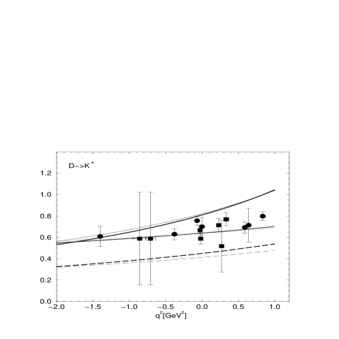
Figure 7.11: The form factors $V(q^{2})$ (solid line), $A_{1}(q^{2})$ (dotted line) and $A_{2}(q^{2})$ (long-dashed line), where the thick (thin) lines represent the HO (linear) parameters, for $D\to\rho$ transition compared with the lattice calculation [110] of $A_{1}(q^{2})$ (data). 7.12: The form factors $V(q^{2})$, $A_{1}(q^{2})$ and $A_{2}(q^{2})$ for $D\to K^{*}$ transition compared with the lattice calculations [105] (square) and [110] (circle) of $A_{1}(q^{2})$. The same line code as in Fig. 7.11 is used.

(3) $D^{0}\to\rho^{-}\ell^{+}\nu_{\ell}$: Our predicted decay rate for $D\to\rho$ in $q^{+}$=0 frame is $\Gamma(D^{0}\to\rho^{-}\ell^{+}\nu_{\ell})$= 6.38 (6.61)$|V_{cd}|^{2}\times 10^{-2}$ ps^-1 for the HO (linear) parameters. We also obtain the ratio $\Gamma_{L}/\Gamma_{T}$, where the subscript $L$ represents the longitudinal polarization and $T$ transverse polarization, for the HO (linear) parameters as 1.39 (1.48), which is quite comparable to the QCD sum rule result: 1.31$\pm$0.11 in Ref. [114]. Our predictions for the branching ratio given by

$${\rm Br}(D^{0}\to\rho^{-}\ell^{+}\nu_{\ell}) = (1.33\pm 0.19)\%\;\;{\rm(HO)},$$ (7.30)

$$= (1.38\pm 0.19)\%\;\;{\rm(Linear)},$$

are overall in a good agreement with the available experimental data [49]: ${\rm Br}_{\rm exp.}=(1.87\pm 0.9)\%$. We show in Table 7.6 our values of $V$, $A_{1}$ and $A_{2}$ at both $q^{2}$=0 and $q^{2}$=$q^{2}_{\rm max}$ and compare with Eq. (7.27) as well as other theoretical predictions. As one can see in Table 7.6, our analytic solutions for the form factors $V(q^{2}_{\rm max})$= 1.006 (1.002), $A_{1}(q^{2}_{\rm max})$=0.572 (0.563) and $A_{2}(q^{2}_{\rm max})$=0.419 (0.357) for the HO (linear) parameters are well approximated by Eq. (7.27), $V_{\Lambda_{1}\Lambda_{2}}(q^{2}_{\rm max})$=1.007 (1.018), $A_{1\Lambda_{1}\Lambda_{2}}(q^{2}_{\rm max})$=0.571 (0.561) and $A_{2\Lambda_{1}\Lambda_{2}}(q^{2}_{\rm max})$=0.420 (0.357). Our analytic solutions are also well fitted by the simple pole formular, $V_{\Lambda_{1}}(q^{2}_{\rm max})$=1.039 (1.036), $A_{1\Lambda_{1}}(q^{2}_{\rm max})$=0.570 (0.559) and $A_{2\Lambda_{1}}(q^{2}_{\rm max})$=0.428 (0.362). This again means that the simple pole formular may be a good approximation to fit the form factors $V$, $A_{1}$ and $A_{2}$. In Fig. 7.11, we present our $q^{2}$ dependence of the form factors $V(q^{2})$ (solid line), $A_{1}(q^{2})$ (dotted line) and $A_{2}(q^{2})$ (long-dashed line) obtained from $q^{+}$=0 frame, where the thick and thin lines represent the HO and linear parameters, respectively. We also compare our $A_{1}(q^{2})$ with the available lattice result [110] (data) and show they are overall in a good agreement with each other.

(4) $D^{0}\to K^{*-}\ell^{+}\nu_{\ell}$: Our predicted decay rate for $D\to K^{*}$ in $q^{+}$=0 frame is $\Gamma(D^{0}\to K^{*-}\ell^{+}\nu_{\ell})$=5.86 (5.85)$|V_{cs}|^{2}\times 10^{-2}$ ps^-1 for the HO (linear) parameters. We obtain the ratio $\Gamma_{L}/\Gamma_{T}$ as 1.37 (1.42) for the HO (linear) parameters, while the available experimental data reported as 1.18$\pm$0.18$\pm$0.08 (E653) [136] and 1.20$\pm$0.13$\pm$0.13 (E687) [137]. Our predictions for the branching ratio given by

$${\rm Br}(D^{0}\to K^{*-}\ell^{+}\nu_{\ell}) = (2.63\pm 0.81)\%\;\;{\rm(HO)},$$ (7.31)

$$= (2.62\pm 0.81)\%\;\;{\rm(Linear)},$$

are quite comparable to the available experimental data [49]: ${\rm Br}_{\rm exp.}$=$(2.02\pm 0.33)\%$. We summarize in Table 7.6 our results of the form factors $V$, $A_{1}$ and $A_{2}$ at both $q^{2}$=0 and $q^{2}$=$q^{2}_{\rm max}$ and compare with the available experimental data [135] as well as Eq. (7.27) and other theoretical results. While our form factors $A_{1}(0)$=0.640 (0.638) and $A_{2}(0)$=0.450 (0.414) for the HO (linear) parameters are quite comparable with the data, $A_{1}(0)=0.58\pm 0.03$ and $A_{2}(0)$=$0.41\pm 0.05$ [135]. our form factor $V(0)$=0.809 (0.822) underestimates the current data, $V(0)$=$1.07\pm 0.09$ [135]. As one can see in Table 7.6, our analytic solutions for the form factors $V(q^{2}_{\rm max})$=1.029 (1.024), $A_{1}(q^{2}_{\rm max})$=0.698 (0.683) and $A_{2}(q^{2}_{\rm max})$=0.534 (0.475) for the HO (linear) parameters are well approximated not only by Eq. (7.27), $V_{\Lambda_{1}\Lambda_{2}}(q^{2}_{\rm max})$=1.029 (1.024), $A_{1\Lambda_{1}\Lambda_{2}}(q^{2}_{\rm max})$=0.698 (0.683) and $A_{2\Lambda_{1}\Lambda_{2}}(q^{2}_{\rm max})$=0.534 (0.475), but also by the simple pole formular, $V_{\Lambda_{1}}(q^{2}_{\rm max})$=1.042 (1.033), $A_{1\Lambda_{1}}(q^{2}_{\rm max})$=0.697 (0.681) and $A_{2\Lambda_{1}}(q^{2}_{\rm max})=0.538(0.477)$. Our simple pole masses $\Lambda_{1}$=2.06 and 2.15 GeV (see Table 7.6) for both HO and linear parameters, respectively, are also in good agreement with the value of $D^{*\pm}_{s}$=2.11 GeV. We also present in Fig. 7.12 our $q^{2}$ dependence of the form factors $V(q^{2})$, $A_{1}(q^{2})$ and $A_{2}(q^{2})$ and compare our $A_{1}(q^{2})$ with the available lattice result [110] (data). Our results of $A_{1}(q^{2})$ for both HO and linear parameter cases are in a good agreement with that of Ref. [110].

(5) $D_{s}\to\eta(\eta^{\prime})\ell^{+}\nu_{\ell}$: These two semileptonic decays are very interesting processes to check our LFQM predictions of $\eta$-$\eta^{\prime}$ mixing angle. In our previous analysis of quark potential model [13] in Chapter 4, we predicted the $\eta$-$\eta^{\prime}$ mixing angle for the HO (linear) potential model as $\theta^{\eta-\eta^{\prime}}_{SU(3)}$=$-19.3^{\circ}(-19.6^{\circ})$.

Our predicted decay rates for $D_{s}\to\eta$ and $D_{s}\to\eta^{\prime}$ in $q^{+}$=0 frame are $\Gamma(D_{s}\to\eta)$= 0.100 (0.104)$\cos^{2}\delta|V_{cs}|^{2}$ ps^-1 and $\Gamma(D_{s}\to\eta^{\prime})$= 0.026 (0.028)$\sin^{2}\delta|V_{cs}|^{2}$ ps^-1, respectively, for the HO (linear) parameters. Using the lifetime $\tau_{D_{s}}$=0.467$\pm$0.017 ps, we obtain the branching ratio for $\theta_{SU(3)}$=$-19^{\circ}$ as follows:

$${\rm Br}(D_{s}\to\eta\ell^{+}\nu_{\ell})=(1.7\pm 0.5)\%,$$

$${\rm Br}(D_{s}\to\eta^{\prime}\ell^{+}\nu_{\ell})=(8.7\pm 2.7)\times 10^{-3}\hskip 5.69046pt{\rm(HO)},$$

$${\rm Br}(D_{s}\to\eta\ell^{+}\nu_{\ell})=(1.8\pm 0.6)\%,$$

$${\rm Br}(D_{s}\to\eta^{\prime}\ell^{+}\nu_{\ell})=(9.3\pm 2.9)\times 10^{-3}\hskip 5.69046pt{\rm(Linear)}.$$ (7.32)

While the experimental data [49] are ${\rm Br}_{\rm exp.}(D_{s}\to\eta\ell^{+}\nu_{\ell})$=(2.5$\pm$0.7)$\%$ and ${\rm Br}_{\rm exp.}(D_{s}\to\eta^{\prime}\ell^{+}\nu_{\ell})$=(8.8$\pm$3.4)$\times 10^{-3}$, respectively. Our results for the $\eta^{\prime}$ decay mode are in a good agreement with the experimental data for both HO and linear parameters. For the $\eta$ decay mode, our values are rather smaller than the central value of the experimental data, neverthless, are quite comparable with the data within the given uncertainties of CKM matrix, $V_{cs}$.

Table 7.8: Summary of the parameters for the $D_{s}\to\eta(\eta^{\prime})$ and $D_{s}\to\phi$ transitions. Note that $c_{\eta}$=$|\cos\delta_{P}|$ and $c_{\eta^{\prime}}$=$|\sin\delta_{P}|$.

	$D_{s}$$\to$$\eta$ $[\eta^{\prime}]$		$D_{s}$$\to$$\phi(s\bar{s})$
	$F$	$f_{+}$	$V$	$A_{1}$	$A_{2}$
HO	$F(0)$	0.692$c_{\eta}$ [0.692$c_{\eta^{\prime}}$]	0.830	0.597	0.409
	$F(q^{2}_{\rm max})$	1.31$c_{\eta}$ [0.93$c_{\eta^{\prime}}$]	1.070	0.672	0.492
	$\Lambda_{1}$ [GeV]	1.94 [1.94]	1.94	2.83	2.25
	$s_{2}\Lambda_{2}$ [GeV]	2.68 [2.68]	2.69	4.80	3.00
	${\cal F}_{\Lambda_{1}}(q^{2}_{\rm max})$	1.49$c_{\eta}$ [0.95$c_{\eta^{\prime}}$]	1.091	0.673	0.498
	${\cal F}_{\Lambda_{1}\Lambda_{2}}(q^{2}_{\rm max})$	1.27$c_{\eta}$ [0.92$c_{\eta^{\prime}}$]	1.069	0.672	0.491
Linear	$F(0)$	0.721$c_{\eta}$ [0.721$c_{\eta^{\prime}}$]	0.861	0.608	0.385
	$F(q^{2}_{\rm max})$	1.28$c_{\eta}$ [0.94$c_{\eta^{\prime}}$]	1.080	0.668	0.445
	$\Lambda_{1}$ [GeV]	2.06 [2.06]	2.05	3.22	2.53
	$s_{2}\Lambda_{2}$ [GeV]	2.94 [2.94]	2.94	-12.91	3.31
	${\cal F}_{\Lambda_{1}}(q^{2}_{\rm max})$	1.37$c_{\eta}$ [0.95$c_{\eta^{\prime}}$]	1.095	0.666	0.448
	${\cal F}_{\Lambda_{1}\Lambda_{2}}(q^{2}_{\rm max})$	1.24$c_{\eta}$ [0.93$c_{\eta^{\prime}}$]	1.079	0.666	0.445
LAT [106]	$F(0)$	0.67(7)$c_{\eta}$ [0.67(7)$c_{\eta^{\prime}}$]	0.86$\pm$0.10	0.52$\pm$0.03	0.17$\pm$0.17
[109]	$F(0)$	$\cdots$ [$\cdots$]	1.30$\pm$0.32(43)	0.73$\pm$0.12(24)	0.55$\pm$0.10(24)

Figure 7.13: The form factor $f_{+}(q^{2})$ for the $D_{s}\to\eta$ transition with the $\eta$-$\eta^{\prime}$ mixing angle $\theta_{SU(3)}$=$-19^{\circ}$. The same line code as in Fig. 7.2 is used for our results. 7.14: The form factor $f_{+}(q^{2})$ for the $D_{s}\to\eta^{\prime}$ transition with the $\eta$-$\eta^{\prime}$ mixing angle $\theta_{SU(3)}$=$-19^{\circ}$. The same line code as in Fig. 7.2 is used for our results.

In Table 7.8, we compare our form factors $f^{D_{s}\eta}_{+}(q^{2})$ and $f^{D_{s}\eta^{\prime}}_{+}(q^{2})$ at both $q^{2}$=0 and $q^{2}$=$q^{2}_{\rm max}$ with Eq. (7.27) and the lattice calculation in Ref. [106]. Our predictions of $f^{D_{s}\eta}_{+}(0)$=0.692 (0.721)$c_{\eta}$ and $f^{D_{s}\eta^{\prime}}_{+}(0)$=0.692 (0.721)$c_{\eta^{\prime}}$ are in good agreement with the lattice results, $f^{D_{s}\eta}_{+}(0)$=(0.67$\pm$ 0.07)$c_{\eta}$ and $f^{D_{s}\eta^{\prime}}_{+}(0)$=(0.67$\pm$ 0.07)$c_{\eta}$ [106], respectively. As one can see in Table 7.8, our analytic solutions $f^{D_{s}\eta}_{+}(q^{2}_{\rm max})$= 1.31 (1.28)$c_{\eta}$ and $f^{D_{s}\eta^{\prime}}_{+}(q^{2})$= 0.93 (0.94)$c_{\eta^{\prime}}$ for the HO (linear) parameters are well approximated by Eq. (7.27), ${\cal F}^{D_{s}\eta}_{\Lambda_{1}\Lambda_{2}}(q^{2}_{\rm max})$=1.27 (1.24)$c_{\eta}$ and ${\cal F}^{D_{s}\eta}_{\Lambda_{1}\Lambda_{2}}(q^{2}_{\rm max})$=0.92 (0.93)$c_{\eta^{\prime}}$, respectively. From the results of the simple pole approximation, ${\cal F}^{D_{s}\eta}_{\Lambda_{1}}(q^{2})$=1.49 (1.37)$c_{\eta}$ and ${\cal F}^{D_{s}\eta^{\prime}}_{\Lambda_{1}}(q^{2})$=0.95 (0.95)$c_{\eta^{\prime}}$, one can find that $\Lambda_{i}(i\geq 2)$ can be neglected for the $D_{s}\to\eta^{\prime}$ transition but not for the $D_{s}\to\eta$ case. For comparison, we also present in Table 7.9 the results obtained from $\theta_{SU(3)}$=$-10^{\circ}$ and $-23^{\circ}$ in $q^{+}$=0 frame. Although it is not easy to conclude which mixing angle is the best from Table 7.9, we can see at least that our predictions with the mixing angle of $\theta^{\eta-\eta^{\prime}}_{SU(3)}$$\approx$$-19^{\circ}$ are overall in a good agreement with the available experimental data. The difference of the decay rates between the $q^{+}$=0 and $q^{+}$$\neq$0 frames is larger for the $\eta$ decay mode (19$\%$ for HO and 18$\%$ for linear) than for the $\eta^{\prime}$ decay mode (12$\%$ for HO and 11$\%$ for linear). Likewise, comparing the form factors $f_{-}(0)$ for the two decay modes given by Table 7.7, one can see that the difference between the $q^{+}$=0 and $q^{+}$$\neq$0 frames is much larger for the $\eta$ decay mode (80$\%$ for HO and 70$\%$ for linear) than for the $\eta^{\prime}$ decay mode (4$\%$ for HO and 2$\%$ for linear). In Figs. 7.13 and 7.14, we present the $q^{2}$ dependence of the form factors $f_{+}(q^{2})$ for $D_{s}\to\eta$ and $D_{s}\to\eta^{\prime}$ with the mixing angle $\theta_{SU(3)}$=$-19^{\circ}$, respectively.

Table 7.9: Branching ratio of the $D_{s}\to\eta,\eta^{\prime}$ transitions for various $\eta-\eta^{\prime}$ mixing angles, $\theta_{SU(3)}=\delta_{P}+35.26^{\circ}$.

Processes		$\theta_{SU(3)}=-10^{\circ}$	$\theta_{SU(3)}=-19^{\circ}$	$\theta_{SU(3)}=-23^{\circ}$	Expt.
$D_{s}\to\eta$	HO	$(2.5\pm 0.8)\%$	$(1.7\pm 0.5)\%$	$(1.4\pm 0.4)\%$	$(2.5\pm 0.7)\%$
	Linear	$(2.6\pm 0.8)\%$	$(1.8\pm 0.6)\%$	$(1.5\pm 0.5)\%$
$D_{s}\to\eta^{\prime}$	HO	$(6.7\pm 2.1)\cdot 10^{-3}$	$(8.7\pm 2.7)\cdot 10^{-3}$	$(9.6\pm 3.0)\cdot 10^{-3}$	$(8.8\pm 3.4)\cdot 10^{-3}$
	Linear	$(7.1\pm 2.2)\cdot 10^{-3}$	$(9.3\pm 2.9)\cdot 10^{-3}$	$(10.0\pm 3.1)\cdot 10^{-3}$

(6) $D_{s}\to\phi\ell^{+}\nu_{\ell}$: Our predicted decay rate for $D_{s}\to\phi(s\bar{s})$ in $q^{+}$=0 frame is $\Gamma(D_{s}\to\phi\ell^{+}\nu_{\ell})$= 4.99 (5.14)$|V_{cs}|^{2}\times 10^{-2}$ ps^-1 for the HO (linear) parameters. We obtain the ratio $\Gamma_{L}/\Gamma_{T}$ as 1.33 (1.37) for the HO (linear) parameters, while the lattice QCD calculation in Ref. [106] reported 1.49$\pm$0.19. Our predictions for the branching ratio are given by

$${\rm Br}(D_{s}\to\phi\ell^{+}\nu_{\ell}) = (2.51\pm 0.77)\%\;\;{\rm(HO)},$$ (7.33)

$$= (2.59\pm 0.80)\%\;\;{\rm(Linear)},$$

where we used $\delta_{V}=-3.3^{\circ}$ for $\omega$-$\phi$ mixing angle. Our results in Eq. (7.33) are quite comparable to the available experimental data [49], ${\rm Br}_{\rm exp.}$=$(2.0\pm 0.5)\%$, within the given uncertainties of the CKM matrix, $V_{cs}$.

Figure 7.15: The form factors $V(q^{2})$, $A_{1}(q^{2})$ and $A_{2}(q^{2})$ for $D_{s}\to\phi(s\bar{s})$ transition. The same line code as in Fig. 7.11 is used.

We summarize in Table 7.8 our results of the form factors $V$, $A_{1}$ and $A_{2}$ at both $q^{2}$=0 and $q^{2}$=$q^{2}_{\rm max}$ and compare with Eq. (7.27) and the lattice results [106, 109]. Our results of the form factors $V$, $A_{1}$ and $A_{2}$ at $q^{2}$=0 are quite comparable with the lattice calculations in Refs. [106, 109]. As one can see in Table 7.8, our analytic solutions for the form factors $V(q^{2}_{\rm max})$=1.070 (1.080), $A_{1}(q^{2}_{\rm max})$=0.672 (0.666) and $A_{2}(q^{2}_{\rm max})$=0.492 (0.445) for the HO (linear) parameters are well approximated not only by Eq. (7.27), $V_{\Lambda_{1}\Lambda_{2}}(q^{2}_{\rm max})$=1.069 (1.079), $A_{1\Lambda_{1}\Lambda_{2}}(q^{2}_{\rm max})$=0.672 (0.666) and $A_{2\Lambda_{1}\Lambda_{2}}(q^{2}_{\rm max})$=0.491 (0.445), but also by the simple pole formular, $V_{\Lambda_{1}}(q^{2}_{\rm max})$=1.091 (1.095), $A_{1\Lambda_{1}}(q^{2}_{\rm max})$=0.673 (0.666) and $A_{2\Lambda_{1}}(q^{2}_{\rm max})=0.498(0.448)$. The simple pole approximation is already enough good approximation for $D_{s}\to\phi$ transition. We also present in Fig. 7.15 our $q^{2}$ dependence of the form factors $V(q^{2})$, $A_{1}(q^{2})$ and $A_{2}(q^{2})$.

7.4.3 $B$ and $B_{s}$ decays

(1) $B^{0}\to\pi^{-}\ell^{+}\nu_{\ell}$: Our predicted decay rate for $B\to\pi$ in $q^{+}=0$ frame is $\Gamma(B^{0}\to\pi^{-}\ell^{+}\nu_{\ell})=7.06(8.16)|V_{ub}|^{2}$ ps^-1 for the HO (linear) parameters. Using the lifetime $\tau_{B_{0}}=1.56\pm 0.04$ ps and $|V_{ub}|=(3.3\pm 0.4\pm 0.7)\times 10^{-3}$[138], our predictions for the branching ratio given by

$${\rm Br}(B^{0}\to\pi^{-}\ell^{+}\nu_{\ell}) = (1.20\pm 0.29)\times 10^{-4}\hskip 5.69046pt{\rm(HO)},$$ (7.34)

$$= (1.40\pm 0.34)\times 10^{-4}\hskip 5.69046pt{\rm(Linear)},$$

are quite comparable wiht the recent experimental data [138], ${\rm Br}(B\to\pi^{-}\ell^{+}\nu_{\ell})$=$(1.8\pm 0.6)\times 10^{-4}$, within the given error range. We also performed the calculations of the decay rate using the valence contributions from $q^{+}$$\neq$0 frame and found that the decay rate obtained from $q^{+}$$\neq$0 frame is about 9 (7)$\%$ smaller for the HO (linear) parameters than the result obtained from $q^{+}$=0 frame.

Table 7.10: Summary of the parameters for the $B\to\pi$ and $B\to\rho$ transitions. The APE [105] and ELC [111] results are from their method ‘b’, which uses the heavy quark scaling laws to extrapolate from $D$- to $B$-mesons at fixed $\omega$.

	$B\to\pi$		$B\to\rho$
	$F$	$f_{+}$	$V$	$A_{1}$	$A_{2}$
HO	$F(0)$	0.234	0.273	0.216	0.196
	$F(q^{2}_{\rm max})$	3.34	0.703	0.449	0.857
	$\Lambda_{1}$ [GeV]	4.37	4.35	6.91	4.70
	$s_{2}\Lambda_{2}$ [GeV]	4.74	5.84	11.01	6.40
	${\cal F}_{\Lambda_{1}}(q^{2}_{\rm max})$	$-0.61$	$-3.66$	0.376	2.43
	${\cal F}_{\Lambda_{1}\Lambda_{2}}(q^{2}_{\rm max})$	1.60	0.972	0.359	0.599
Linear	$F(0)$	0.273	0.324	0.249	0.220
	$F(q^{2}_{\rm max})$	2.80	0.688	0.461	0.851
	$\Lambda_{1}$ [GeV]	4.59	4.57	8.06	5.09
	$s_{2}\Lambda_{2}$ [GeV]	6.53	7.11	14.62	7.02
	${\cal F}_{\Lambda_{1}}(q^{2}_{\rm max})$	$-1.07$	13.00	0.362	1.026
	${\cal F}_{\Lambda_{1}\Lambda_{2}}(q^{2}_{\rm max})$	2.16	1.736	0.358	0.573
LAT [104]	$F(0)$	0.27$\pm$0.11	0.35${}^{+0.06}_{-0.05}$	0.27${}^{+0.05}_{-0.04}$	0.26${}^{+0.05}_{-0.03}$
	$F(q^{2}_{\rm max})$	$\cdots$	2.07${}^{+0.11}_{-0.06}$	0.46${}^{+0.02}_{-0.01}$	0.88${}^{+0.05}_{-0.03}$
[105]	$F(0)$	0.35$\pm$0.08	0.53$\pm$0.31	0.24$\pm$0.12	0.27$\pm$0.80
[111]	$F(0)$	0.30$\pm$0.14(5)	0.37$\pm$0.11	0.22$\pm$0.05	0.49$\pm$0.21(5)
SR [112]	$F(0)$	$\cdots$	0.34$\pm$0.05	0.26$\pm$0.04	0.22$\pm$0.03
[113]	$F(0)$	$\cdots$	0.35$\pm$0.07	0.27$\pm$0.05	0.28$\pm$0.05

Table 7.11: Comparison of the form factors $f_{-}(q^{2})$ at $q^{2}$=0 between $q^{+}$=0 and $q^{+}$$\neq$0 frames. The differences between the two frames are the measure of the nonvalence contributions in $q^{+}$$\neq$0 frame.

Models		$B\to\pi$	$B\to D$	$B_{s}\to D_{s}$
HO	$q^{+}$=0	$-0.203$	$-0.318$	$-0.305$
	$q^{+}$$\neq$0	$-0.235$	$-0.478$	$-0.518$
Linear	$q^{+}$=0	$-0.238$	$-0.328$	$-0.325$
	$q^{+}$$\neq$0	$-0.273$	$-0.499$	$-0.533$

We summarize in Table 7.10 our analytic solutions of $f^{B\pi}_{+}$ obtained at both $q^{2}$=0 and $q^{2}$=$q^{2}_{\rm max}$ and compare with Eq. (7.27) as well as other theoretical results. As one can see in Table 7.10, our results of $f^{B\pi}_{+}(0)$ for both HO and linear parameters are quite comparable with the lattice QCD calculations [104, 105, 111]. Comparing with the pole dominace formular given by Eq. (7.27), we found that our solution of $f^{B\pi}_{+}(q^{2}_{\rm max})$=3.34 (2.80) for the HO (linear) parameters are neither fitted by Eq. (7.27), ${\cal F}_{\Lambda_{1}\Lambda_{2}}(q^{2}_{\rm max})$=1.60 (2.16), nor by the simple pole approximation, ${\cal F}_{\Lambda_{1}}(q^{2}_{\rm max})$=$-0.61$ $(-1.07)$. Even though we do not know yet how many terms of $\Lambda_{i}(i\geq 3)$ are needed to obtain the well approximated solutions motivated by the pole dominace model, it seems quite clear that the pole approximation up to $\Lambda_{2}$ given by Eq. (7.27) does not work well for the heavy-to-light transitions. In Table 7.11, we also summarize the results of the form factor $f_{-}(0)$ at $q^{2}$=0 obtained from both $q^{+}$=0 and $q^{+}$$\neq$0 frames. The difference, i.e., nonvalence contribution from $q^{+}$$\neq$0 frame, of $f^{B\pi}_{-}(0)$ between the two frames is about 16 (15)$\%$ for the HO (linear) parameters.

In Figs. 7.16(a) and 7.16(b), we present the $q^{2}$ dependence of the form factors $f^{B\pi}_{+}(q^{2})$ and $f^{B\pi}_{0}(q^{2})$ obtained from both $q^{+}$=0 (thick lines) and $q^{+}$$\neq$0 (thin lines) frames, respectively, and compare with the available lattice QCD calculations [108]. Again, the nonvalence contributions from $q^{+}$$\neq$0 frame are quite sizeable especially for $f^{DK}_{0}(q^{2})$ case. Our analytic solutions of $f^{B\pi}_{+}(q^{2})$ for both HO and linear parameters are overall in a good agreement with the lattice calculations in Ref. [108].

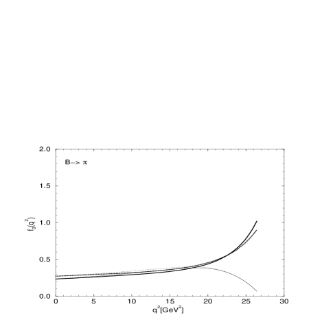
Figure 7.16: (a) The form factor $f_{+}(q^{2})$ for the $B\to\pi$ transition compared with the lattice calculation [108] (data). The same line code as in Fig. 7.2 is used for our results. (b) The form factor $f_{0}(q^{2})$ for the $B\to\pi$ transition. The same line code is used as in (a).

Figure 7.17: (a) The form factor $V(q^{2})$ for the $B^{0}\to\rho$ transition. The thick (thin) solid line corresponds to our HO (linear) parameters. For comparison, we include the results of ${\cal F}_{\Lambda_{1}\Lambda_{2}}(q^{2})$ (dashed line) given by Eq. (7.27) and lattice QCD from UKQCD [103] ($\bullet$), APE [105] (square) and ELC [111] ($\diamond$). (b) The form factor $A_{1}(q^{2})$ for the $B^{0}\to\rho$ transition. The same line code as in (a) is used.

Figure 7.17: (c) The form factor $A_{2}(q^{2})$ for the $B^{0}\to\rho$ transition. The same line code as in (a) is used.

(2) $B^{0}\to\rho^{-}\ell^{+}\nu_{\ell}$: Our predicted decay rate for $B\to\rho$ in $q^{+}$=0 frame is $\Gamma(B^{0}\to\rho^{-}\ell^{+}\nu_{\ell})$= 11.44 (14.25)$|V_{ub}|^{2}$ ps^-1 for the HO (linear) parameters. We obtain the ratio $\Gamma_{L}/\Gamma_{T}$ as 1.07 (1.19) for the HO (linear) parameters, while other QM calculations predicted as 0.3 [81], 1.34 [118] and 1.13 [123]. The lattice QCD of Ref. [104] and the QCD sum rule of Ref. [113] also calculated the ratio as 0.80${}^{+0.04}_{-0.03}$ and 0.52$\pm$0.08, respectively. Our predictions for the branching ratio are given by

$${\rm Br}(B^{0}\to\rho^{-}\ell^{+}\nu_{\ell}) = (1.94^{+1.51}_{-1.08})\times 10^{-4}\;\;{\rm(HO)},$$ (7.35)

$$= (2.36^{+1.84}_{-0.52})\times 10^{-4}\;\;{\rm(Linear)}.$$

While the central value of linear parameters is quite comparable to the available experimental data [49], ${\rm Br}_{\rm exp.}$=$(2.5^{+0.8}_{-1.0})\times 10^{-4}$, the central value of the HO parameters underestimates the data.

We summarize in Table 7.10 our results of the form factors $V$, $A_{1}$ and $A_{2}$ at both $q^{2}$=0 and $q^{2}$=$q^{2}_{\rm max}$ and compare with Eq. (7.27) and other theoretical results. Our results of the form factors $V$, $A_{1}$ and $A_{2}$ at $q^{2}$=0 are in good agreement with the lattice calculations in Refs. [104, 105, 111] as well as the QCD sum rule in Refs. [112, 113]. Moreover, our results of the axial vector form factors $A_{1}(q^{2}_{\rm max})$=0.449 (0.461) and $A_{2}(q^{2}_{\rm max})$=0.857 (0.851) for the HO (linear) parameters are in excellent agreement with the lattice results in Ref. [104]: $A_{1}(q^{2}_{\rm max})$=0.46${}^{+0.02}_{-0.01}$ and $A_{2}(q^{2}_{\rm max})$=0.88${}^{+0.05}_{-0.03}$, respectively. Our prediction of the vector form factor $V(q^{2}_{\rm max})$=0.703 (0.688) for the HO(linear) parameters, however, disagree with the lattice result in Ref. [104], $V(q^{2}_{\rm max})$=2.07${}^{+0.11}_{-0.06}$. As one can see in Table 7.10, our analytic solutions for the form factors $V(q^{2}_{\rm max})$ and $A_{2}(q^{2}_{\rm max})$ are neither approximated by Eq. (7.27) nor the simple pole formular, i.e., ${\cal F}_{\Lambda_{1}}(q^{2}_{\rm max})$. Only the form factor of $A_{1}$ is reasonably approximated (but still $\sim 20\%$ difference from our analytic solution) by the simple pole dominace, i.e., $A_{1\Lambda_{1}}(q^{2}_{\rm max})$=0.376 (0.362) for the HO (linear) parameters with the pole mass $\Lambda_{1}$= 6.91 (8.06) GeV. It is interesting to note that UKQCD [103] in their analysis showed the simple pole behavior for $A_{1}(q^{2})$ is preferred with $m_{\rm pole}=7^{+2}_{-1}$ GeV, which is quite compatible with our values of $\Lambda_{1}$.

In Figs. 7.17(a), 17(b) and 17(c), we show the $q^{2}$ dependence of the form factors $V$, $A_{1}$ and $A_{2}$, respectively, and compare with the available lattice results [103, 105, 111]. For comparison, we also include in Fig. 7.17(a) the result (dashed line) of Eq. (7.27), i.e., ${\cal F}_{\Lambda_{1}\Lambda_{2}}(q^{2})$ obtained from the linear parameters. As one can see in Figs. 7.17(a) and 17(b), our analytic solutions for the $A_{1}(q^{2})$ and $A_{2}(q^{2})$ are in excellent agreement with the lattice calculations [103, 105, 111]. For the vector form factor $V(q^{2})$ case, our analytic solution gives reasonable agreement with the ELC result [111] ($\diamond$) but underestimates the result of UKQCD [103] ($\bullet$).

(3) $B(B_{s})\to D(D_{s})\ell\nu_{\ell}$: Our predicted decay rates for $B\to D$ and $B_{s}\to D_{s}$ in $q^{+}$=0 frame are $\Gamma(B^{0}\to D^{-}\ell^{+}\nu_{\ell})$= 8.93 (9.39)$|V_{cb}|^{2}$ ps^-1 and $\Gamma(B_{s}\to D_{s}^{-}\ell^{+}\nu_{\ell})$= 8.80 (9.30)$|V_{cb}|^{2}$ ps^-1, respectively, for the HO (linear) parameters. Using $\tau_{B_{s}}$=(1.54$\pm$0.07) ps and $|V_{bc}|$=0.0395$\pm$0.003 [49], we obtain the branching ratio as follows:

$${\rm Br}(B^{0}\to D^{-}\ell^{+}\nu_{\ell})=(2.17\pm 0.19)\%,$$

$${\rm Br}(B_{s}\to D_{s}^{-}\ell^{+}\nu_{\ell})=(2.11\pm 0.18)\%\hskip 5.69046pt{\rm(HO)},$$

$${\rm Br}(B^{0}\to D^{-}\ell^{+}\nu_{\ell})=(2.28\pm 0.20)\%,$$

$${\rm Br}(B_{s}\to D_{s}^{-}\ell^{+}\nu_{\ell})=(2.23\pm 0.20)\%\hskip 5.69046pt{\rm(Linear)}.$$ (7.36)

Our predictions of the $B\to D$ transition for both HO and linear cases are in a good agreement with the experimental data [49], ${\rm Br}(B^{0}\to D^{-}\ell^{+}\nu_{\ell})$=(2.00$\pm$0.25)$\%$. The decay rates of $B\to D$ and $B_{s}\to D_{s}$ obtained from the valence contributions in $q^{+}\neq 0$ frame for the HO (linear) parameters are about 6 (6)$\%$ and 8 (8)$\%$ larger than those obtained from $q^{+}$=0 frame, respectively.

Table 7.12: Summary of the parameters for the $B\to D(B_{s}\to D_{s})$ and $B\to D^{*}(B_{s}\to D^{*}_{s})$ transitions. The experimental data for $B\to D^{*}$ transition was obtained by assuming an exponential dependence of the form factors on $q^{2}$ according to the formalism outline in Ref. [80].

	$B\to D(B_{s}\to D_{s})$		$B\to D^{*}(B_{s}\to D^{*}_{s})$
	$F$	$f_{+}$	$V$	$A_{1}$	$A_{2}$
HO	$F(0)$	0.686 (0.664)	0.711 (0.692)	0.652 (0.619)	0.581 (0.541)
	$F(q^{2}_{\rm max})$	1.11 (1.13)	1.10 (1.11)	0.80 (0.80)	0.86 (0.84)
	$\Lambda_{1}$ [GeV]	5.22 (4.95)	5.25 (4.94)	7.74 (6.77)	5.49 (5.15)
	$s_{2}\Lambda_{2}$ [GeV]	7.35 (6.64)	7.45 (6.62)	$-19.17$ (10.07)	7.81 (6.88)
	${\cal F}_{\Lambda_{1}}(q^{2}_{\rm max})$	1.20 (1.26)	1.16 (1.22)	0.79 (0.81)	0.90 (0.90)
	${\cal F}_{\Lambda_{1}\Lambda_{2}}(q^{2}_{\rm max})$	1.11 (1.11)	1.10 (1.11)	0.79 (0.79)	0.86 (0.83)
Linear	$F(0)$	0.709 (0.689)	0.727 (0.717)	0.667 (0.638)	0.580 (0.549)
	$F(q^{2}_{\rm max})$	1.12 (1.14)	1.10 (1.13)	0.80 (0.80)	0.83 (0.82)
	$\Lambda_{1}$ [GeV]	5.38 (5.09)	5.39 (5.08)	8.24 (7.16)	5.70 (5.35)
	$s_{2}\Lambda_{2}$ [GeV]	7.77 (6.93)	7.82 (6.91)	$-13.68$ (11.46)	8.29 (7.24)
	${\cal F}_{\Lambda_{1}}(q^{2}_{\rm max})$	1.19 (1.24)	1.15 (1.22)	0.79 (0.80)	0.86 (0.87)
	${\cal F}_{\Lambda_{1}\Lambda_{2}}(q^{2}_{\rm max})$	1.12 (1.13)	1.10 (1.12)	0.79 (0.80)	0.83 (0.82)
ISGW [80]	$F(q^{2}_{\rm max})$	$\cdots$	1.20 ($\cdots$)	0.94 ($\cdots$)	1.08 ($\cdots$)
BSW [118]	$F(q^{2}_{\rm max})$	$\cdots$	0.97 ($\cdots$)	0.85 ($\cdots$)	0.90 ($\cdots$)
EXP. [148]	$F(q^{2}_{\rm max})$	$\cdots$	0.91$\pm$0.49$\pm$0.12	0.85$\pm$0.07$\pm$0.11	0.87$\pm$0.22$\pm$0.10

We summarize in Table 7.12 our analytic solutions of $f^{BD}_{+}$ and $f^{B_{s}D_{s}}_{+}$ obtained at both $q^{2}$=0 and $q^{2}$=$q^{2}_{\rm max}$ and compare with Eq. (7.27). As one can see in Table 7.12, our results of $f^{BD}_{+}(q^{2}_{\rm max})$=1.11 (1.12) and $f^{B_{s}D_{s}}_{+}(q^{2}_{\rm max})$=1.13 (1.14) for the HO (linear) parameters are well approximated by Eq. (7.27), ${\cal F}^{BD}_{\Lambda_{1}\Lambda_{2}}(q^{2}_{\rm max})$=1.11 (1.12) and ${\cal F}^{B_{s}D_{s}}_{\Lambda_{1}\Lambda_{2}}(q^{2}_{\rm max})$=1.11 (1.13). The results of the monopole approximations, ${\cal F}^{BD}_{\Lambda_{1}}(q^{2}_{\rm max})$=1.20 (1.19) and ${\cal F}^{B_{s}D_{s}}_{\Lambda_{1}}(q^{2}_{\rm max})$=1.26 (1.24) are also quite comparable to our analytic solutions. The form factors $f^{BD}_{-}(0)$ and $f^{B_{s}D_{s}}_{-}(0)$ obtained from $q^{+}$=0 frame are also summarized in Table 7.11 and compared with those obtained from $q^{+}$$\neq$0 frame. As one can see in Table 7.11, the results of $f^{BD}_{-}(0)$ and $f^{B_{s}D_{s}}_{-}(0)$ in $q^{+}$$\neq$0 frame are about 50 (52)$\%$ and 70 (64)$\%$ larger for the HO (linear) parameters than those in $q^{+}$=0 frame, respectively.

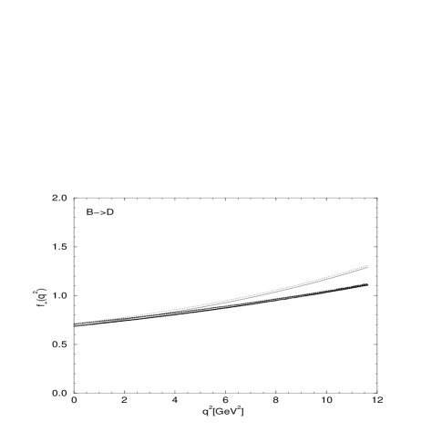
Figure 7.18: (a) The form factor $f_{+}(q^{2})$ for $B$$\to$$D$ transition. The same line code as in Fig. 7.2 is used. (b) The form factor $f_{0}(q^{2})$ for $B$$\to$$D$ transition. The same line code as in Fig. 7.2 is used.

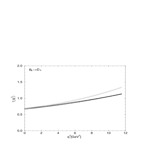
Figure 7.19: (a) The form factor $f_{+}(q^{2})$ for $B_{s}$$\to$$D_{s}$ transition. The same line code as in Fig. 7.2 is used. (b) The form factor $f_{0}(q^{2})$ for $B_{s}$$\to$$D_{s}$ transition. The same line code as in Fig. 7.2 is used.

In Figs. 7.18 and 7.19, we show the $q^{2}$ dependence behaviors of the form factors $f_{+}$ and $f_{0}$ for $B\to D$ and $B_{s}\to D_{s}$ transitions, respectively. For comparison, we also include the results of the valence contributions in $q^{+}$$\neq$0 frame. For these heavy-to-heavy transition cases, we can easily see the nonvalence contributions (i.e., the difference of the results between the two frames) are much suppressed compared to the previous light-to-light and heavy-to-light transition cases.

These heavy-to-heavy transitions are also used to investigate model reliability by checking the universal IW function given by Eq. (7.7) in heavy-quark symmetry. The slope $\rho^{2}$ of the IW function at the zero-recoil point is defined as

$$\xi(w)=1-\rho^{2}(w-1),$$ (7.37)

where $w=v_{1}\cdot v_{2}=(M^{2}_{1}+M^{2}_{2}-q^{2})/(2M_{1}M_{2})$. Our predictions of the slope $\rho^{2}=0.80\leq\rho^{2}\leq 0.92$ for possible combinations of $\beta_{D}$ and $\beta_{B}$ are quite comparable with the current world average $\rho^{2}_{\rm avg.}$=0.66$\pm$0.19 [49] extracted from exclusive semileptonic ${\bar{B}}\to D\ell{\bar{\nu}}$ decay as well as other theoretical estimates, $0.7\leq\rho^{2}\leq 0.88$ in [123] and $0.87$ in [139]. In Fig. 7.20, our predictions of the IW function $\xi^{BD}(v_{1}\cdot v_{2})$ for the HO (solid) with the common gaussian $\beta=\beta_{B}$=0.496 and linear (dotted line) parameters with the common $\beta=\beta_{B}$=0.5266, respectively, are compared with the available experimental data [140, 141] and show good agreement with the data. Other combinations of the gaussian $\beta$ paramters give very similar $q^{2}$ behavior to those as shown in Fig. 7.20.

Figure 7.20: The IW function $\xi^{BD}(v_{1}\cdot v_{2})$ for the HO (solid) with the common gaussian $\beta=\beta_{B}$=0.496 and linear (dotted line) parameters with the common $\beta=\beta_{B}$=0.5266, respectively. We compare our results with the experimental data of ARGUS [140] (square) and CLEO [141] (circle).

(2) $\bar{B}^{0}(\bar{B}^{0}_{s})\to D^{*+}(D^{*+}_{s})\ell^{-}\bar{\nu}_{\ell}$: Our predicted decay rates for $B\to D^{*}$ and $B_{s}\to D_{s}$ in $q^{+}$=0 frame are $\Gamma(\bar{B}^{0}\to D^{*+}\ell^{-}\bar{\nu}_{\ell})$= 22.13 (22.90)$|V_{bc}|^{2}$ ps^-1 and $\Gamma(\bar{B}^{0}_{s}\to D^{*+}_{s}\ell^{-}\bar{\nu}_{\ell})$= 21.34 (22.25)$|V_{bc}|^{2}$ ps^-1 for the HO (linear) parameters, respectively. The ratio $\Gamma_{L}/\Gamma_{T}$ for $B\to D$ and $B_{s}\to D_{s}$ decays are obtained as 1.20 (1.23) and 1.19 (1.21) for the HO (linear) parameters, respectively. While the experimental data for $B\to D^{*}$ reported as 0.85$\pm$0.45 [142] and 0.82$\pm$0.36 [143].

Figure 7.21: The $d\Gamma/dq^{2}$ distribution for $\bar{B}\to D^{*}\ell\bar{\nu}$ decays using the linear parameters. The thick solid, dotted, and long-dashed lines are the results from the central value, upper limit, and the lower limit of the CKM matrix element, $|V_{bc}|$=0.0395$\pm$0.003, respectively. The experimental data are taken from Ref. [147].

Our predictions for the branching ratio are given by

$${\rm Br}(\bar{B}^{0}\to D^{*+}\ell^{-}\bar{\nu}_{\ell})=(5.39\pm 0.82)\%,$$

$${\rm Br}(\bar{B}^{0}_{s}\to D^{*+}_{s}\ell^{-}\bar{\nu}_{\ell})=(5.13\pm 0.75)\%\hskip 5.69046pt{\rm(HO)},$$

$${\rm Br}(\bar{B}^{0}\to D^{*+}\ell^{-}\bar{\nu}_{\ell})=(5.58\pm 0.85)\%,$$

$${\rm Br}({\bar{B}}^{0}_{s}\to D^{*+}_{s}\ell^{-}\bar{\nu}_{\ell})=(5.35\pm 0.78)\%\hskip 5.69046pt{\rm(Linear)}.$$ (7.38)

Even though the current average value for $B^{0}\to D^{*}$ decays, ${\rm Br}_{\rm exp.}(\bar{B}^{0}\to D^{*+}\ell^{-}\bar{\nu}_{\ell})$ =$(4.60\pm 0.27)\%$, is smaller than our predictions, it is interesting to note that the recent experiments [144, 145, 146] reported results close to our predictions, i.e., $(5.08\pm 0.21\pm 0.66)\%$ [144], $(5.53\pm 0.26\pm 0.52)\%$ [145], and $(5.52\pm 0.17\pm 0.68)\%$ [146], respectively. In Fig. 7.21, we present the differential rate for $B\to D^{*}$ decays using the linear parameters and compare with the available experimental data [147]. Within the uncertainties of the CKM matrix element $|V_{bc}|$=0.0395$\pm$0.003, our results are overall in good agreement with the data. The results for the HO parameters are not much different from those for the linear parameters.

We summarize in Table 7.12 our analytic solutions of $V$, $A_{1}$ and $A_{2}$ obtained at both $q^{2}$=0 and $q^{2}$=$q^{2}_{\rm max}$ and compare with Eq. (7.27) as well as the available experimental data [148] and other theoretical results [80, 118]. As one can see in Table 7.12, our results of the three form factors for $B\to D^{*}$ transition, i.e., $V(q^{2}_{\rm max})$=1.10 (1.10), $A_{1}(q^{2}_{\rm max})$=0.80 (0.80) and $A_{2}(q^{2}_{\rm max})$=0.86 (0.83) for the HO (linear) parameters are in good agreement with the experimental data [148], $V_{\rm exp.}(q^{2}_{\rm max})$=0.91$\pm$0.49$\pm$0.12, $A_{1{\rm exp.}}(q^{2}_{\rm max})$=0.85$\pm$0.07$\pm$0.11 and $A_{2{\rm exp.}}(q^{2}_{\rm max})$=0.87$\pm$0.22$\pm$0.10, respectively. Our analytic solutions are also well approximated by not only Eq. (7.27) but also the monopole form factor ${\cal F}_{\Lambda_{1}}$ (see Table 7.12). In Figs. 7.22 and 7.23, we show the $q^{2}$ dependence behaviors of the three form factors for $B\to D^{*}$ and $B_{s}\to D^{*}_{s}$ decays, respectively.

Figure 7.22: The form factors $V(q^{2})$, $A_{1}(q^{2})$ and $A_{2}(q^{2})$ for $B\to D^{*}$ transition. The same line code as in Fig. 7.11 is used. 7.23: The form factors $V(q^{2})$, $A_{1}(q^{2})$ and $A_{2}(q^{2})$ for $B\to D^{*}_{s}$ transition. The same line code as in Fig. 7.11 is used.

Experimentally, two form-factor ratios for $B\to D^{*}$ decays defined by [132, 149]

$$R_{1}(q^{2})=\biggl{[}1-\frac{q^{2}}{(M_{B}+M_{D^{*}})^{2}}\biggl{]}\frac{V(q^{2})}{A_{1}(q^{2})},$$

$$R_{2}(q^{2})=\biggl{[}1-\frac{q^{2}}{(M_{B}+M_{D^{*}})^{2}}\biggl{]}\frac{A_{2}(q^{2})}{A_{1}(q^{2})},$$ (7.39)

have been measured by CLEO [149] as follows: $R_{1}(q^{2}_{\rm max})=1.24\pm 0.26\pm 0.12$ and $R_{2}(q^{2}_{\rm max})=0.72\pm 0.18\pm 0.07$. From Table 7.12, we obtain the ratios as $R_{1}(q^{2}_{\rm max})$=1.10 (1.11) and $R_{1}(q^{2}_{\rm max})$=0.86 (0.84) for the HO (linear) parameters, which are in good agreement with the data. Our results are also agree with the predictions of Neubert [132], $R_{1}(q^{2}_{\rm max})$=1.35 and $R_{2}(q^{2}_{\rm max})$=0.79, and the ISGW2 model [81], $R_{1}(q^{2}_{\rm max})$=1.27 and $R_{2}(q^{2}_{\rm max})$=1.01. In Fig. 7.24, we present the two form-factor ratios $R_{1}$ and $R_{2}$ as a function of $w$ and compare with the data [149] at $q^{2}=q^{2}_{\rm max}$(or $w$=1) anticipating more data in the entire physical $q^{2}$ range. Our results show almost $w$ independent behavior as indicated by Ref. [132].

Figure 7.24: The two form-factor ratios, $R_{1}(w)$ (solid line) and $R_{2}(w)$ (dotted line) for the HO parameters compared with the experimental data [149] of $R_{1}(1)$ (circle) and $R_{2}(1)$ (square). 7.25: Our predictions of the ratio of $\xi^{BD}(w)/\xi^{BD^{*}}(w)$ for both HO (solid line) and linear (dotted line) parameters compared with the experimental data [49].

The form factors for $0^{-}\to 1^{-}$ transitions in the heavy-quark limit are also related to the IW function via

$$\xi(w) = \frac{2\sqrt{M_{P}M_{D}}}{M_{P}+M_{D}}V(q^{2})=\frac{2\sqrt{M_{P}M_{D}}}{M_{P}+M_{D}}A_{2}(q^{2})$$ (7.40)

$$= \frac{2\sqrt{M_{P}M_{D}}}{M_{P}+M_{D}}\frac{A_{1}(q^{2})}{[1-q^{2}/(M_{P}+M_{D})^{2}]}.$$

The slope of the IW function at zero-recoil for the $B\to D^{*}$ decays is obtained as $0.85\leq\rho^{2}\leq 0.97$ for all possible combinations of the gaussian parameters $\beta_{B}$ and $\beta_{D^{*}}$. Our results are in good agreement with the data: $\rho^{2}$=0.91$\pm$0.15$\pm$0.06 (CLEO) [149] and $\rho^{2}_{\rm avg.}$=0.71$\pm$0.11 (PDG) [49]. We present in Fig. 7.25 the ratio of the two IW functions for $B\to D$ and $B\to D^{*}$, i.e., $\xi^{BD}(w)/\xi^{BD^{*}}(w)$, where $\xi^{BD}(w)$ and $\xi^{BD^{*}}(w)$ is obtained by the form factors $f_{+}(q^{2})$ and $V(q^{2})$, respectively, and compare with the data [49]. Our results for both HO (solid line) and linear (dotted line) parameters are almost equal to 1, the value expected from the heavy quark limit ($m_{b},m_{c}\to\infty$) and thus show a good agreement with the data [49].

Moreover, the decay $\bar{B}^{0}\to D^{*+}\ell^{-}\bar{\nu}_{\ell}$ allows one to measure the chirality of the weak $b\to c$ transition [132, 140, 149, 150], which is only possible if the daughter meson has spin $J>0$. This $b\to c$ chirality can be tested by measuring the forward-backward asymmetry [132, 140, 148, 150]:

$$A_{\rm FB} = \frac{3}{4}\frac{\int K_{f}(q^{2})q^{2}(|H_{-}|^{2}-|H_{-}|^{2})dq^{2}dp_{\ell}}{\int K_{f}(q^{2})q^{2}(|H_{+}|^{2}+|H_{-}|^{2}+|H_{0}|^{2})dq^{2}dp_{\ell}},$$ (7.41)

$$= \frac{3}{4}\frac{\Gamma_{-}-\Gamma_{+}}{\Gamma}.$$

The helicity alignment of the $W^{-}$ is given by [140]

$$A_{\rm pol}=2\frac{\Gamma_{0}}{\Gamma_{+}+\Gamma_{-}}-1,$$ (7.42)

which describes the $D^{*+}$ polarization extracted from the $D^{*+}$ decay angle distribution (see for more detail in Ref. [132, 150]). From Eqs. (7.41) and (2.1), we obtain $A^{BD^{*}}_{\rm FB}$= 0.195 (0.193) and $A^{BD^{*}}_{\rm pol}$= 1.396 (1.510) for the HO (linear) parameters. Our results for $B\to D^{*}$ are in excellent agreement with the available experimental data: $A_{\rm FB}$=0.20$\pm$0.08$\pm$0.06, $A_{\rm pol}$=1.1$\pm$0.4$\pm$0.2 [140] and $A_{\rm FB}$=0.197$\pm$0.033$\pm$0.016, $A_{\rm pol}$=1.55$\pm$0.26$\pm$0.13 [149]. Similarly, we also obtain $A^{B_{s}D^{*}_{s}}_{\rm FB}$= 0.194 (0.194) and $A^{B_{s}D^{*}_{s}}_{\rm pol}$= 1.376 (1.422) for the HO (linear) parameters anticipating future experimental data for $B_{s}\to D^{*}_{s}$. Finally, we summarize in Table 7.13 and 7.14 our results of the decay rates for $0^{-}\to 0^{-}$ and $0^{-}\to 1^{-}$ transitions, respectively.

Table 7.13: Decay rate $\Gamma$ (in unit of ps^-1) and branching ratio ${\rm Br}(0^{-}\to 0^{-}\ell\nu_{\ell})$ for various semileptonic decays. We use $\theta^{\eta-\eta^{\prime}}_{SU(3)}$=$-19^{\circ}$ to obtain the branching ratio for $D_{s}$$\to$$\eta(\eta^{\prime})$ decays. The used CKM matrix elements are $|V_{cs}|$=1.04$\pm$0.16, $|V_{cd}|$=0.224$\pm$0.016, $|V_{ub}|$=(3.3$\pm$0.4$\pm$0.7)$\times$10^-3, and $|V_{bc}|$=0.0395$\pm$0.003 [49].

Mode		$\Gamma$	Br.	Expt.(Br.)
$D\to\pi$	HO	0.110$|V_{cd}|^{2}$	$(2.30\pm 0.33)\cdot 10^{-3}$	$(3.7\pm 0.6)\cdot 10^{-3}$
	Linear	0.113$|V_{cd}|^{2}$	$(2.36\pm 0.34)\cdot 10^{-3}$
$D\to K$	HO	8.26$\cdot 10^{-2}|V_{cs}|^{2}$	$(3.71\pm 1.14)\%[e^{+}\nu_{e}]$	$(3.66\pm 0.18)\%$
		6.40$\cdot 10^{-2}|V_{cs}|^{2}$	$(2.87\pm 0.88)\%[\mu^{+}\nu_{\mu}]$	for $D^{0}\to K^{-}e^{+}\nu_{e}$
	Linear	8.36$\cdot 10^{-2}|V_{cs}|^{2}$	$(3.75\pm 1.16)\%[e^{+}\nu_{e}]$	$(3.23\pm 0.17)\%$
		6.43$\cdot 10^{-2}|V_{cs}|^{2}$	$(2.89\pm 0.90)\%[\mu^{+}\nu_{\mu}]$	for $D^{0}\to K^{-}\mu^{+}\nu_{\mu}$
$D_{s}\to\eta$	HO	0.100$\cos^{2}\delta|V_{cs}|^{2}$	$(1.7\pm 0.5)\%$	$(2.5\pm 0.7)\%$
	Linear	0.104$\cos^{2}\delta|V_{cs}|^{2}$	$(1.8\pm 0.6)\%$
$D_{s}\to\eta^{\prime}$	HO	0.026$\sin^{2}\delta|V_{cs}|^{2}$	$(8.7\pm 2.7)\cdot 10^{-3}$	$(8.8\pm 3.4)\cdot 10^{-3}$
	Linear	0.028$\sin^{2}\delta|V_{cs}|^{2}$	$(9.3\pm 2.9)\cdot 10^{-3}$
$B\to\pi$	HO	7.06$|V_{ub}|^{2}$	$(1.20\pm 0.29)\cdot 10^{-4}$	$(1.8\pm 0.6)\cdot 10^{-4}$
	Linear	8.16$|V_{ub}|^{2}$	$(1.40\pm 0.34)\cdot 10^{-4}$
$B\to D$	HO	8.93$|V_{cb}|^{2}$	$(2.17\pm 0.19)\%$	$(2.00\pm 0.25)\%$
	Linear	9.39$|V_{cb}|^{2}$	$(2.28\pm 0.20)\%$
$B_{s}\to D_{s}$	HO	8.80$|V_{cb}|^{2}$	$(2.11\pm 0.18)\%$	–
	Linear	9.30$|V_{cb}|^{2}$	$(2.23\pm 0.20)\%$

Table 7.14: Decay rate $\Gamma$ (in unit of $|V_{q_{1}q_{2}}|^{2}$ ps^-1) and branching ratio ${\rm Br}(0^{-}\to 1^{-}\ell\nu_{\ell})$ for various semileptonic decays. We use $|\delta_{V}|$=3.3^∘ to obtain the branching ratio for $D_{s}\to\phi$ decays. The $\Gamma_{L}$ and $\Gamma_{T}$ are the decay rates for the longitudinal and transverse helicity contributions, respectively.

Mode		$\Gamma$	$\Gamma_{L}/\Gamma_{T}$	Br.	Expt.(Br.)
$D^{0}\to K^{*}$	HO	5.856$\cdot 10^{-2}$	1.37	$(2.63\pm 0.81)\%$	$(2.02\pm 0.33)\%$
	Linear	5.846$\cdot 10^{-2}$	1.42	$(2.62\pm 0.81)\%$
$D^{0}\to\rho^{-}$	HO	6.382$\cdot 10^{-2}$	1.39	$(1.33\pm 0.19)\cdot 10^{-3}$	$(1.87\pm 0.9)\cdot 10^{-3}$
	Linear	6.610$\cdot 10^{-2}$	1.47	$(1.38\pm 0.19)\cdot 10^{-3}$
$D_{s}\to\phi$	HO	4.994$\cdot 10^{-2}$	1.33	$(2.51\pm 0.77)\%$	$(2.0\pm 0.5)\%$
	Linear	5.137$\cdot 10^{-2}$	1.37	$(2.59\pm 0.80)\%$
$B^{0}\to\rho^{-}$	HO	11.445	1.07	$(1.94^{+1.51}_{-1.08})\cdot 10^{-4}$	$(2.5^{+0.8}_{-1.0})\cdot 10^{-4}$
	Linear	14.254	1.19	$(2.36^{+1.84}_{-0.52})\cdot 10^{-4}$
$B^{0}\to D^{*}$	HO	22.133	1.20	$(5.39\pm 0.82)\%$	$(4.60\pm 0.27)\%$
	Linear	22.904	1.23	$(5.58\pm 0.85)\%$
$B^{0}_{s}\to D^{*}_{s}$	HO	21.341	1.19	$(5.13\pm 0.75)\%$	–
	Linear	22.253	1.21	$(5.35\pm 0.78)\%$

7.5 Summary and Discussion

In conclusion, in this Chapter, we analyzed the exclusive $0^{-}$$\to$$0^{-}$ and $0^{-}$$\to$$1^{-}$ semileptonic heavy meson decays extending our LFQM constrained by the variational principle for the QCD-motivated effective Hamiltonian disscussed in Chapter 4. Our model not only provided overall a good agreement with the available experimental data and the lattice QCD results for the weak transition form factors and branching ratios of the light-to-light ($K_{\ell 3}$), heavy-to-light and heavy-to-heavy meson decays but also rendered a large number of predictions to the heavy meson mass spectra and decay constants. Our predicted meson mass spectra given by Table 7.3 were overall in a good agreement with the data [49]. Our values of the decay constants given by Table 7.4 were also in a good agreement with the results of lattice QCD [102, 107] anticipating future accurate experimental data.

As an application of our model, we first calculated the spacelike EM form factors of $D$ and $B$ mesons as well as $\pi$ and $K$ mesons in $q^{+}$=0 frame and estimated the nonvalence contributions of the EM form factors from the $q^{+}$$\neq$0 frame by comparing the valence contributions obtained from the $q^{+}$$\neq$0 frame with those obtained from the $q^{+}$=0 frame. The nonvalence contributions from the $q^{+}$$\neq$0 frame are highly suppressed as the quark mass increases, i.e., in the order of $\pi>K>D>B$, as one can see from Figs. 7.2-7.5.

We have overcome the difficulty associated with the nonvalence Z-graph contribution in timelike region by the analytic continuation of weak form factors from the spacelike region. In other words, the form factors $f_{\pm}$ for $0^{-}\to 0^{-}$ decays and the form factors $V$, $A_{1}$ and $A_{2}$ were obtained in the $q^{+}$=0 frame and then analytically continued to the timelike region by changing $q_{\perp}$ to $iq_{\perp}$ in the form factors. The matrix element of the $``\perp"$ component of the current $J^{\mu}$ was used to obtain the form factor $f_{-}$, since the $J^{-}$ is not immune to the zero mode contributions even in the $q^{+}$=0 frame [26]. Our numerical computation confirmed the equivalence of our analytic continuation method and the dispersion relation method [123]. The nonvalence contributions from the $q^{+}$$\neq$0 were also quantified for the $0^{-}\to 0^{-}$ decays by comparing the valence contributions between the $q^{+}$=0 and $q^{+}$$\neq$0 frames. Another interesting thing is that our predicted value of the $\eta$-$\eta^{\prime}$ mixing angle, i.e., $\theta_{SU(3)}\approx-19^{\circ}$, works fairly well for the predicitions of the decay rates for $D_{s}\to\eta(\eta^{\prime})$ processes.

Furthermore, our analytic solutions of the form factors for both $0^{-}\to 0^{-}$ and $0^{-}\to 1^{-}$ decays are well approximated by monopole-type form factors except heavy-to-light processes such as $B\to\pi$ and $B\to\rho$. For these two processes, our analytic solutions of the form factors are neither approximated by monopole-type form factors nor the Eq. (7.27). In order to explain the discrepancies between our analytic solutions and the approximations of the pole dominace model, more accurate experimental data or the lattice results should be accomodated. Nonetheless, if we assume the pole dominance model is a good approximation for the heavy-to-light decays, this may indicate that our LQFM with a simple picture of $q\bar{q}$ contents for the description of a meson is not valid for really high $q^{2}$ region. Anyway, the comparison between our analytic solutions and the results of the pole dominance model provides a good testing ground for the validity of our model calculations.

Chapter 8 Conclusion

In this thesis, we have investigated the electroweak form factors and the semileptonic decays of pseudoscalar and vector mesons within the framework of light-front constituent quark model. In Chapters 2 and 3 of this thesis, we have discussed the two different schemes in treating the meson masses, e.g., SM and IM schemes. Regardless of the difference between the two schemes, once the best fit parameters were used, both schemes provided the predictions that were not only pretty similar with each other but also remarkably good compared to the available experimental data for form factors, decay constants, chargi radii, etc., of various light pseudoscalar and vector mesons as well as their radiative decay widths. Similarly, once the best fit parameters were chosen, the difference from the Jacobi factor in the IM model wave functions is substantially reduced in the numerical predictions for the physical observables. However, the difference in the choice of the radial wave function, e.g., harmonic-oscillator (HO) wave function versus power-law (PL) wave function, was appreciable no matter what parameters were used. For example, in the phenomenology of various meson radiative decays at low $Q^{2}$, we observed that the Gaussian type wave function was clearly better than the PL wave function in comparison with the available experimental data.

In order to justify the model wave function as a solution of the QCD-inspired dynamic equation, we applied the variational principle in Chapter 4 of this thesis to the QCD-motivated potential, which includes not only the Coulomb plus confining potential but also the hyperfine interaction, to obtain the correct $\rho$-$\pi$ splitting. For the confining potential, we took both HO ($\sim r^{2}$) and linear ($\sim r$) type potentials and compared the numerical results for these two cases. The variational principle for the effective Hamiltonian turns out to be crucial to find the optimum values of our model parameters as shown in Chapters 4 and 7. We adopted the IM scheme to assure the orthogonality of model wave functions. As shown in Figs. 4.1(a) and 4.1(b), our central potentials for both HO and linear potentials in Eq. (4.2) are not only very similar to each other but also quite close to the Isgur-Scora-Grinstein-Wise model 2(ISGW2) [81] potentials. Using our quark potential model discussed in Chapter 4, we predicted the ground state meson spectra (see Table 7.3). Our predictions of ground state meson mass spectra agreed quite well with the experimental data [49] (within 6$\%$ error). Furthermore, our model predicted the two unmeasured mass spectra of ${}^{1}S_{0}(b\bar{b})$ and ${}^{3}S_{1}(b\bar{s})$ systems as $M_{b\bar{b}}$=9295 (9657) MeV and $M_{b\bar{s}}$=5471 (5424) MeV for the HO (linear) potential, respectively.

We have also predicted the $\omega$-$\phi$ and $\eta$-$\eta^{\prime}$ mixing angles using the parametrization to incorporate the quark annihilation diagrams [47, 75, 76] mediated by gluon exchanges and the SU(3) symmetry breaking, i.e., $m_{u}(d)\neq m_{s}$. Our results of the $\omega$-$\phi$ and $\eta$-$\eta^{\prime}$ mixing angles are $|\delta_{V}|\approx 4.2^{\circ}(7.8^{\circ})$ and $\theta_{SU(3)}\approx-19.3^{\circ}(-19.6^{\circ})$ for the HO (linear) potential model, respectively. The sensitivity of the ($\omega,\phi$) mass spectra for $\sim 1^{\circ}(5^{\circ})$ variation of $\delta_{V}$, i.e., from $\delta_{V}=4.2^{\circ}(7.8^{\circ})$ to $3.3^{\circ}$ for the HO (linear) potential case, is within the $1\%(5\%)$ level. As we discussed in the appendix E, the sign of mixing angle depends on the sign of SU(3) breaking parameter $X$ (see Eqs. (E.3)-(E.5)). While $X_{P}>0$ is well supported by the Particle Data Group [49] ($-23^{\circ}\leq\theta^{\eta-\eta^{\prime}}_{SU(3)}\leq-10^{\circ}$), the sign of $X_{V}$ is not yet definite at the present stage of phenomenology. Regarding the sign of $X_{V}$, it is interesting to note that $\delta_{V}\approx-3.3^{\circ}(=\theta_{SU(3)}-35.26^{\circ})$ (i.e., $X_{V}<0$) is favored in Refs. [10, 83, 84, 85], while the conventional Gell-Mann-Okubo mass formula for the exact SU(3) limit ($X\to 1$) predicts $\delta_{V}\approx 0^{\circ}$ in the linear mass scheme and $\delta_{V}\approx+3.3^{\circ}$ (i.e., $X_{V}>0$) in the quadratic mass scheme [49]. Even though it is not yet clear which sign of $\omega$-$\phi$ mixing angle should be taken, the overall agreement between our HO potential model with the positive sign, i.e., $\delta_{V}\sim+3.3^{\circ}$, and the available experimental data seem to be quite good. If we were to choose the sign of $X$ as $X>0$ in Eq. (E.4), then the fact that the mass difference $m_{\omega}-m_{\rho}$ is positive is correlated with the sign of the $\omega$-$\phi$ mixing angle [92]. In other words, $m_{\omega}>m_{\rho}$ implies $\delta_{V}>0$ from Eqs. (E.3)-(E.5). Perhaps, the precision measurement of $\phi\to\eta^{\prime}\gamma$ envisioned in the future at TJNAF experiments might be helpful to give a more stringent test of $\delta_{V}$. We also predicted the decay constants for various pseudoscalar and vector mesons as summarized in Tables 4.3 and 7.4. Our predictions for the decay constants are quite consistent with the available experimental data [49] as well as the lattice QCD [102, 107]. For the heavy meson decay constants, however, the current experimental data have large error-bars and the more accurate data are needed.

We further applied our quark potential model to compute the radiative (see Chapter 4) and the semileptonic (see Chapter7) decays of pseudoscalar and vector mesons. One of the distinguished features in our LF approach is the ability to compute the timelike form factors as shown in $0^{-}\to 0^{-}$ and $0^{-}\to 1^{-}$ semileptonic decays. While we calculated the exclusive processes in the Drell-Yan-West ($q^{+}$=0) frame, we analytically continued the amplitudes to the timelike region. Our analytic continuation method (i.e. changing $q_{\perp}$ to $iq_{\perp}$ in the form factors) avoided encountering the nonvalence diagram (black blob in Fig. 1.1(b)) and yielded the outcome of timelike form factors. As summarized in Tables 7.13 and 7.14 for the $0^{-}\to 0^{-}$ and $0^{-}\to 1^{-}$ semileptonic decays, respectively, our numerical results for both HO and linear parameters were overall not only quite similar to each other but also in good agreement with the available experimental data [49]. To assure our method of analytic continuation, we used the exactly solvable model of scalar field theory interacting with gauge fields and analyzed the full information for the nonvalence diagram. As shown in Chapter 5, we were able to check if the analytic continuation of the results in the $q^{+}$=0 frame (without the black blob) indeed reproduces the exact results in timelike region. We established that this method can actually broaden the applicability of the standard LF frame à la Drell-Yan-West to the timelike form factor calculation. Exploring the timelike region, we have also found the importance of zero-mode contributions. The estimation of the zero-mode contribution was presented in Chapter 6. To the extent that the zero-modes have a significant contribution to some physical observables [41], it seems conceivable that the condensation of zero-modes could lead to the nontrivial realization of chiral symmetry breaking in the LF quantization approach.

Throughout the thesis, we attempted to fill the gap between the model wave function and the QCD-motivated potential and explore covering as many observables as possible. We think that the success of our model hinges on the advantage of LF quantization realized by the rational energy-momentum dispersion relation. It is crucial to calculate the “good” components of the current in the reference frame which deletes the complication from the nonvalence Z-graph contribution. We anticipate further stringent tests of our model with more accurate data from future experiments and lattice QCD calculations.

Appendix A Spin-Orbit Wave Functions ${\cal R}_{\lambda\bar{\lambda}}^{JJ_{3}}(x,{\bf k}_{\perp})$

The $4\times 4$ Dirac matrices $\gamma_{\mu}$ are given by

$$\gamma^{\mu}\gamma^{\nu}+\gamma^{\nu}\gamma^{\mu}=2g^{\mu\nu}$$ (A.1)

with $\gamma^{0}$ hermitian and $\gamma^{i}$ antihermitian. In the chiral representation[10]

$$\gamma^{0}\>=\>\left(\begin{array}[]{cc}0&I\\ I&0\end{array}\;\right),\;\gamma^{i}=\left(\begin{array}[]{cc}0&\sigma^{i}\\ -\sigma^{i}&0\end{array}\;\;\right),$$ (A.2)

where $I$ is the $2\times 2$ unit matrix and $\sigma^{i}$ are Pauli matrices defined as

$$\sigma^{1}\>=\left(\begin{array}[]{cc}0&1\\ 1&0\end{array}\;\right),\;\sigma^{2}=\left(\begin{array}[]{cc}0&-i\\ i&0\end{array}\;\right),\;\sigma^{3}=\left(\begin{array}[]{cc}1&0\\ 0&-1\end{array}\;\right).$$ (A.3)

We frequently need $\gamma^{+}\equiv\gamma^{0}+\gamma^{3}$ and $\gamma^{5}\equiv i\gamma^{0}\gamma^{1}\gamma^{2}\gamma^{3}$, which are given as

$$\gamma^{+}\>=\left(\begin{array}[]{cccc}0&0&2&0\\ 0&0&0&0\\ 0&0&0&0\\ 0&2&0&0\end{array}\;\right),\;\gamma^{5}=\left(\begin{array}[]{cccc}-1&0&0&0\\ 0&-1&0&0\\ 0&0&1&0\\ 0&0&0&1\end{array}\;\right).$$ (A.4)

The constituent quarks are spin $\frac{1}{2}$ particles and can be described by Dirac spinors $u(k,\lambda)$ and $v(k,\lambda)$ satisfying the Dirac equation

$$(/\!\!\!k-m)u(k,\lambda)=0,\;\;\;(/\!\!\!k+m)v(k,\lambda)=0,$$ (A.5)

where $/\!\!\!k=k_{\mu}\gamma^{\mu}$. Using the $\gamma$-matrices given by Eqs. (A.1)-(A.4), we now introduce the spinor basis:

$$u(k,\lambda)=\frac{1}{\sqrt{k^{+}}}(/\!\!\!k+m)u(\lambda),\;\;v(k,\lambda)=\frac{1}{\sqrt{k^{+}}}(/\!\!\!k-m)v(\lambda),$$ (A.6)

$$u\left(\frac{1}{2}\right)\>=\left(\begin{array}[]{c}1\\ 0\\ 0\\ 0\end{array}\;\right),\;\;u\left(-\frac{1}{2}\right)=\left(\begin{array}[]{c}0\\ 0\\ 0\\ 1\end{array}\right),$$ (A.7)

where $v(\lambda)=u(-\lambda)$. We then can derive the spinors $u(k,\lambda)$ and $v(k,\lambda)$ as well as the antispinors $\bar{u}(k,\lambda)$ and $\bar{v}(k,\lambda)$, where we use $\bar{u}=u^{+}\gamma^{0}$ and $\bar{v}=v^{+}\gamma^{0}$, as

$$u\left(k,\frac{1}{2}\right)\>=\frac{1}{\sqrt{k^{+}}}\left(\begin{array}[]{c}m\\ 0\\ k^{+}\\ k^{R}\end{array}\;\right),\;\;u\left(k,-\frac{1}{2}\right)=\frac{1}{\sqrt{k^{+}}}\left(\begin{array}[]{c}-k^{L}\\ k^{+}\\ 0\\ m\end{array}\;\right),$$ (A.8)

$$v\left(k,\frac{1}{2}\right)\>=\frac{1}{\sqrt{k^{+}}}\left(\begin{array}[]{c}-k^{L}\\ k^{+}\\ 0\\ -m\end{array}\right),\;\;v\left(k,-\frac{1}{2}\right)=\frac{1}{\sqrt{k^{+}}}\left(\begin{array}[]{c}-m\\ 0\\ k^{+}\\ k^{R}\end{array}\;\right),$$ (A.9)

$$\bar{u}\left(k,\frac{1}{2}\right)=\frac{1}{\sqrt{k^{+}}}\left(k^{+},k^{L},m,0\right),\;\bar{u}\left(k,-\frac{1}{2}\right)=\frac{1}{\sqrt{k^{+}}}\left(0,m,-k^{R},k^{+}\right),$$ (A.10)

$$\bar{v}\left(k,\frac{1}{2}\right)=\frac{1}{\sqrt{k^{+}}}\left(0,-m,-k^{R},k^{+}\right),\;\bar{v}\left(k,-\frac{1}{2}\right)=\frac{1}{\sqrt{k^{+}}}\left(k^{+},k^{L},-m,0\right).$$ (A.11)

Here, $k^{R}$ and $k^{L}$ are defined as $k^{R}\equiv k^{1}+ik^{2}$ and $k^{L}\equiv k^{1}-ik^{2}$, respectivly. The Melosh transformation ${\cal R}_{M}(x,{\bf k}_{\perp},m)$ transforms the usual instant frame spin basis into the LF frame spin basis and thus enables one to assign proper total angular momentum quantum numbers to hadronic states. In the basis given Eq. (A.8)-(A.11), the spin-orbit wave functions of pseudoscalar and vector mesons can be represented in the following covariant way:

$${\cal R}_{\lambda\bar{\lambda}}^{00}(x,{\bf k}_{\perp})=\frac{-1}{\sqrt{2}[M^{2}_{0}-(m_{1}-m_{2})^{2}]^{1/2}}\bar{u}(p_{1},\lambda)\gamma_{5}v(p_{2},\bar{\lambda}),$$ (A.12)

and

$${\cal R}_{\lambda\bar{\lambda}}^{1J_{3}}(x,{\bf k}_{\perp}) = \frac{-1}{\sqrt{2}[M^{2}_{0}-(m_{1}-m_{2})^{2}]^{1/2}}$$ (A.13)

$$\times \bar{u}(p_{1},\lambda)\biggl{[}/\!\!\!\varepsilon(J_{3})-\frac{\varepsilon\cdot(p_{1}-p_{2})}{M_{0}+m_{1}+m_{2}}\biggr{]}v(p_{2},\bar{\lambda}).$$

The four-vectors $p_{1},p_{2}$ are given in terms of the LF relative momentum variables $(x,{\bf k}_{\perp})$ as follows

$$p^{+}_{1}=xP^{+},\;\;p^{+}_{2}=(1-x)P^{+},$$

$${\bf p}_{1\perp}=x{\bf P}_{\perp}+{\bf k}_{\perp},\;\;{\bf p}_{2\perp}=(1-x){\bf P}_{\perp}-{\bf k}_{\perp},$$ (A.14)

and satisfied by $p^{2}_{i}=m^{2}_{i}(i=1,2)$. The polarization vectors are given by

$$\varepsilon^{\mu}(\pm)=\biggl{[}0,\frac{2}{P^{+}}{\bf\varepsilon}_{\perp}(\pm)\cdot{\bf P}_{\perp},{\bf\varepsilon}_{\perp}(\pm)\biggr{]},$$

$${\bf\varepsilon}_{\perp}(\pm)=\mp(1,\pm i)/\sqrt{2},$$

$$\varepsilon^{\mu}(0)=\frac{1}{M_{0}}\biggl{[}P^{+},\frac{-M^{2}_{0}+P^{2}_{\perp}}{P^{+}},{\bf P}_{\perp}\biggr{]}.$$ (A.15)

The explicit form of Eqs. (A.12) and (A.13) are given by

$${\cal R}^{00}_{\lambda\bar{\lambda}}\>=\frac{{\cal R}_{0}}{\sqrt{2}}\left(\begin{array}[]{cc}-k^{L}&xm_{2}+(1-x)m_{1}\\ -xm_{2}-(1-x)m_{1}&-k^{R}\end{array}\right),\;$$ (A.16)

$${\cal R}^{11}_{\lambda\bar{\lambda}}\>={\cal R}_{0}\left(\begin{array}[]{cc}xm_{2}+(1-x)m_{1}+\frac{k^{2}_{\perp}}{M_{0}+m_{1}+m_{2}}&k^{R}\frac{xM_{0}+m_{1}}{M_{0}+m_{1}+m_{2}}\\ -k^{R}\frac{(1-x)M_{0}+m_{2}}{M_{0}+m_{1}+m_{2}}&-\frac{(k^{R})^{2}}{M_{0}+m_{1}+m_{2}}\end{array}\right),\;$$ (A.17)

$${\cal R}^{10}_{\lambda\bar{\lambda}}\>=\frac{{\cal R}_{0}}{\sqrt{2}}\left(\begin{array}[]{cc}k^{L}\frac{(1-2x)M_{0}+m_{2}-m_{1}}{M_{0}+m_{1}+m_{2}}&xm_{2}+(1-x)m_{1}+\frac{2k^{2}_{\perp}}{M_{0}+m_{1}+m_{2}}\\ xm_{2}+(1-x)m_{1}+\frac{2k^{2}_{\perp}}{M_{0}+m_{1}+m_{2}}&-k^{R}\frac{(1-2x)M_{0}+m_{2}-m_{1}}{M_{0}+m_{1}+m_{2}}\end{array}\right),\;$$ (A.18)

$${\cal R}^{1-1}_{\lambda\bar{\lambda}}\>={\cal R}_{0}\left(\begin{array}[]{cc}-\frac{(k^{L})^{2}}{M_{0}+m_{1}+m_{2}}&k^{L}\frac{(1-x)M_{0}+m_{2}}{M_{0}+m_{1}+m_{2}}\\ -k^{L}\frac{xM_{0}+m_{1}}{M_{0}+m_{1}+m_{2}}&xm_{2}+(1-x)m_{1}+\frac{k^{2}_{\perp}}{M_{0}+m_{1}+m_{2}}\end{array}\right),\;$$ (A.19)

where

$${\cal R}_{0}=\frac{1}{\sqrt{x(1-x)}[M^{2}_{0}-(m_{1}-m_{2})^{2}]^{1/2}},$$ (A.20)

and

$$M^{2}_{0}=\frac{k^{2}_{\perp}+m^{2}_{1}}{x}+\frac{k^{2}_{\perp}+m^{2}_{2}}{1-x}.$$ (A.21)

Appendix B Spin-Averaged Meson Masses of $\eta,\eta^{\prime},\omega$ and $\phi$

We list our flavor wave functions of the neutral pseudoscalar $(\eta,\eta^{\prime})$ and vector $(\omega,\phi)$ nonet states to show explicitly how we obtained the values of spin-averaged mass used in Chapter 2:

$$\eta=\frac{1}{\sqrt{6}}(u\bar{u}+d\bar{d}-2s\bar{s}),$$ (B.1)

$$\eta^{\prime}=\frac{1}{\sqrt{3}}(u\bar{u}+d\bar{d}+s\bar{s}),$$ (B.2)

$$\omega=\frac{1}{\sqrt{2}}(u\bar{u}+d\bar{d}),$$ (B.3)

$$\phi=s\bar{s}.$$ (B.4)

For ideally mixed isocalar and isovector mesons, we take the flavor wave function as

$$\chi_{ns}^{P(V)}=\frac{1}{\sqrt{2}}(u\bar{u}+d\bar{d}),\hskip 14.22636pt\chi_{s}^{P(V)}=s\bar{s},$$ (B.5)

where $P(V)$ denotes pseudoscalar(vector) meson states. In terms of this basis, the neutral meson nonet states are given by

$$\eta_{1}=\sqrt{\frac{2}{3}}\chi_{ns}^{P}+\sqrt{\frac{1}{3}}\chi_{s}^{P},\hskip 14.22636pt\omega_{1}=\sqrt{\frac{2}{3}}\omega+\sqrt{\frac{1}{3}}\phi,$$

$$\eta_{8}=\sqrt{\frac{1}{3}}\chi_{ns}^{P}-\sqrt{\frac{2}{3}}\chi_{s}^{P},\hskip 14.22636pt\omega_{8}=\sqrt{\frac{1}{3}}\omega-\sqrt{\frac{2}{3}}\phi$$ (B.6)

where $\eta=\eta_{8}$, $\eta^{\prime}=\eta_{1}$, $\omega=\chi_{ns}^{V}$ and $\phi=\chi_{s}^{V}$. We define the spin-averaged masses $\bar{M}$ of $\chi_{ns}$ and $\chi_{s}$ as follows:

$$\bar{M}_{ns}=\frac{1}{4}M_{ns}^{P}+\frac{3}{4}M_{ns}^{V},\hskip 14.22636pt\bar{M}_{s}=\frac{1}{4}M_{s}^{P}+\frac{3}{4}M_{s}^{V}.$$ (B.7)

Using Eqs. (B.3)-(B.6), we assign

$$M_{\eta}^{\rm exp}=\frac{1}{3}M_{ns}^{P}+\frac{2}{3}M_{s}^{P},\hskip 8.5359ptM_{\eta^{\prime}}^{\rm exp}=\frac{2}{3}M_{ns}^{P}+\frac{1}{3}M_{s}^{P},\hskip 8.5359ptM_{\omega}^{\rm exp}=M^{V}_{ns},$$

$$M_{\phi}^{\rm exp}=M^{V}_{s}.$$ (B.8)

Then, we obtain the following spin averaged masses of $\eta$ and $\eta^{\prime}$:

$$\bar{M}_{\eta}=\frac{1}{3}\bar{M}_{ns}+\frac{2}{3}\bar{M}_{s}=842\;{\rm MeV},$$ (B.9)

$$\bar{M}_{\eta^{\prime}}=\frac{2}{3}\bar{M}_{ns}+\frac{1}{3}\bar{M}_{s}=885\;{\rm MeV}.$$ (B.10)

Likewise, from Eq. (B.6), we obtain

$$\bar{M}_{\omega_{1}}=\frac{2}{3}\bar{M}_{\omega}+\frac{1}{3}\bar{M}_{\phi},$$ (B.11)

$$\bar{M}_{\omega_{8}}=\frac{1}{3}\bar{M}_{\omega}+\frac{2}{3}\bar{M}_{\phi}.$$ (B.12)

Using $\bar{M}_{\eta}=\bar{M}_{\omega_{8}}$ and $\bar{M}_{\eta^{\prime}}=\bar{M}_{\omega_{1}}$, we can then evaluate the spin-averaged masses of $\omega$ and $\phi$ as $\bar{M}_{\omega}=928$ MeV and $\bar{M}_{\phi}=799$ MeV, respectively.

To calculate the spin-averaged meson masses depending on the schemes of flavor mixing, let’s consider the “perfect mixing”($\theta_{SU(3)}=-10^{\circ}$) $\tilde{\eta}$ and $\tilde{\eta^{\prime}}$ states defined by[47, 48],

$$\tilde{\eta}=\frac{1}{\sqrt{2}}(\chi_{ns}^{P}-\chi_{s}^{P}),\hskip 14.22636pt\tilde{\eta^{\prime}}=\frac{1}{\sqrt{2}}(\chi_{ns}^{P}+\chi_{s}^{P}).$$ (B.13)

Using Eqs. (B.13) and Eq. (B.6), we obtain

$$\eta_{1}=\frac{\sqrt{2}-1}{\sqrt{6}}\tilde{\eta}+\frac{\sqrt{2}+1}{\sqrt{6}}\tilde{\eta^{\prime}},\hskip 14.22636pt\eta_{8}=\frac{1+\sqrt{2}}{\sqrt{6}}\tilde{\eta}+\frac{1-\sqrt{2}}{\sqrt{6}}\tilde{\eta^{\prime}}.$$ (B.14)

Thus, the spin-averaged masses $\bar{m}$ of the $\tilde{\eta}$ and $\tilde{\eta^{\prime}}$ for the “perfect mixing” scheme are related to $\bar{M}_{\eta}$ and $\bar{M}_{\eta^{\prime}}$ calculated in our scheme (see Eqs. (B.9) and (B.10)), respectively, as follows:

$$\bar{M}_{\eta^{\prime}}=\frac{(\sqrt{2}-1)^{2}}{6}\bar{m}_{\tilde{\eta}}+\frac{(\sqrt{2}+1)^{2}}{6}\bar{m}_{\tilde{\eta^{\prime}}},$$

$$\bar{M}_{\eta}=\frac{(\sqrt{2}+1)^{2}}{6}\bar{m}_{\tilde{\eta}}+\frac{(\sqrt{2}-1)^{2}}{6}\bar{m}_{\tilde{\eta^{\prime}}}.$$ (B.15)

From Eq. (B.15), the spin-averaged masses for the “perfect mixing” states are given by $\bar{m}_{\tilde{\eta}}=843$ MeV and $\bar{m}_{\tilde{\eta^{\prime}}}=884$ MeV, respectively. Using the same method as above, for the $\theta_{SU(3)}=-23^{\circ}$ mixing scheme, we obtain the following spin averaged meson masses: $m_{\eta}=838$ MeV and $m_{\eta^{\prime}}=873$ MeV, respectively.

Appendix C The Electromagnetic Decay Width $\Gamma(A\to B+\gamma)$

In this appendix, we derive the decay widths of $A\to B+\gamma$ ($A=\rho,K^{*},\omega,\phi,$ and $B=\pi,K,\eta,\eta^{\prime}$) and $A_{1}\to\pi+\gamma$.

Consider the electromagnetic decay process $A\to B+\gamma$. If the masses of A and B mesons are given by $m_{A}$ and $m_{B}$, respectively, then the decay rate $\Gamma(A\to B+\gamma)$ in the rest frame of $A$ is given by $(\hbar=c=1)$

$$\Gamma(A\to B+\gamma) = \frac{1}{(2\pi)^{6}}\frac{S}{2m_{A}}\int\frac{d^{3}{\bf p}_{B}}{2E_{B}}\frac{d^{3}{\bf p}_{\gamma}}{2E_{\gamma}}|{\cal M}|^{2}(2\pi)^{4}\delta^{3}({\bf p}_{B}+{\bf p}_{\gamma})$$ (C.1)

$$\times \delta(m_{A}-E_{B}-E_{\gamma}),$$

where $S=1/j!$ for each group of $j$ identical particles in the final states. Here, ${\cal M}$ is the transition matrix element defined by

$${\cal M}=\varepsilon_{\mu}^{*}(\lambda_{\gamma})\langle B(P^{\prime})|J^{\mu}|A(P,\lambda)\rangle.$$ (C.2)

To allow decays to all possible spin configurations, we consider the replacement

$$|{\cal M}|^{2}\to{\overline{|{\cal M}|}}^{2}\equiv\frac{1}{2S_{A}+1}\sum_{\lambda_{\gamma}=\pm 1}|{\cal M}|^{2},$$ (C.3)

where $S_{A}$ is the spin of particle A and $\lambda_{\gamma}$ corresponds to the state of transverse polarization of the emitted photon. The above replacement means the average over the initial spin and the sum over the helicities of the emitted photon. Then, from Eq. (C.1), we get

$$\Gamma(A\to B+C) = \frac{S}{2(4\pi)^{2}m_{A}}\frac{1}{2S_{A}+1}\int|{\bf p}_{B}|^{2}d|{\bf p}_{B}|d\Omega$$ (C.4)

$$\times \frac{\delta(m_{A}-\sqrt{m_{B}^{2}+{\bf p}_{B}^{2}}-|{\bf p}_{B}|)}{|{\bf p}_{B}|\sqrt{m_{B}^{2}+{\bf p}_{B}^{2}}}\sum_{\lambda_{\gamma=\pm 1}}|{\cal M}|^{2}.$$

If we let $|{\bf p}_{B}|=\rho$ and $E\equiv\sqrt{m_{B}^{2}+\rho^{2}}+\rho$, then

$$\Gamma(A\to B+\gamma)=\frac{S}{8\pi m_{A}}\frac{1}{2S_{A}+1}\int^{\infty}_{m_{B}}dE\frac{\rho}{E}\delta(m_{A}-E)\sum_{\lambda_{\gamma=\pm 1}}|{\cal M}|^{2}.$$ (C.5)

Therefore, we get

$$\Gamma(A\to B+\gamma) = \frac{S}{8\pi m_{A}^{2}}\frac{\rho_{0}}{2S_{A}+1}\sum_{\lambda_{\gamma=\pm 1}}|{\cal M}|^{2},$$ (C.6)

where

$$S=1,\hskip 14.45377pt{\rm if\hskip 14.45377ptB\neq\gamma},$$

$$S=\frac{1}{2},\hskip 14.45377pt{\rm if\hskip 14.45377ptB=\gamma}.$$ (C.7)

Here, $\rho_{0}$ is the value of $\rho$ when $E=m_{A}$, i.e., $\rho_{0}=(m_{A}^{2}-m_{B}^{2})/2m_{A}$. In the rest frame of $A$, i.e., $P_{A}=(m_{A},{\vec{0}})$ ,$P^{\prime}_{B}=(m_{B},{\bf p}_{B})$ and $P_{\gamma}=(|{\bf p}_{B}|,-{\bf p}_{B})$, the invariant amplitude square is given by

$$\sum_{\lambda_{\gamma=\pm 1}}|{\cal M}|^{2} = \sum_{\lambda_{\gamma=\pm 1}}|eG_{AB}(Q^{2})\epsilon^{\mu\nu\alpha\beta}\varepsilon^{*}_{\mu}(\lambda_{\gamma})\varepsilon_{\nu}(P,\lambda)P^{\prime}_{\alpha}P_{\beta}|^{2}$$ (C.8)

$$= e^{2}|G_{AB}(Q^{2})|^{2}2|\epsilon^{12\alpha\beta}P^{\prime}_{\alpha}P_{\beta}|^{2}=e^{2}|G_{AB}(Q^{2})|^{2}2m_{A}^{2}{\bf p}_{B}^{2}$$

$$= \frac{(m_{A}^{2}-m_{B}^{2})^{2}}{2}e^{2}|G_{AB}(Q^{2})|^{2}.$$

Therefore, we get the following decay width $\Gamma(A\to B+\gamma)$:

$$\Gamma(A\to B+\gamma)=\frac{\alpha}{2S_{A}+1}|G_{AB}(0)|^{2}\biggl{(}\frac{m_{A}^{2}-m_{B}^{2}}{2m_{A}}\biggr{)}^{3},$$ (C.9)

where $\alpha(=e^{2}/4\pi)$ is the fine-structure constant.

The decay width of $A_{1}\to\pi\gamma$ can be calculated in the same manner using our definition of the transition matrix element given by Eq. (2.26) as follows:

$$\sum_{\lambda_{\gamma=\pm 1}}|{\cal M}|^{2}=|\epsilon_{\mu}^{*}(\lambda_{\gamma})\langle\pi(P^{\prime})|J^{\mu}|A_{1}(P,\lambda)\rangle|^{2}=2\biggl{|}e\frac{G_{1}(Q^{2})}{m_{A_{1}}}(P_{A_{1}}+P^{\prime}_{\pi})\cdot P_{\gamma}\biggr{|}^{2}$$

$$\;\;\;=2\biggl{|}e\frac{G_{1}(Q^{2})}{m_{A_{1}}}\biggr{|}{\bf p}_{\pi}|(m_{A_{1}}+m_{\pi}+|{\bf p}_{\pi}|)|^{2}=2e^{2}\biggl{|}\frac{G_{1}(Q^{2})}{m_{A_{1}}}\biggr{|}^{2}(2m_{A_{1}}{\bf p}_{\pi})^{2},$$

and the result is given by

$$\Gamma(A_{1}\to\pi\gamma)=\frac{4\alpha}{3}\biggl{|}\frac{G_{1}(0)}{m_{A_{1}}}\biggr{|}^{2}\biggl{(}\frac{m_{A_{1}}^{2}-m_{\pi}^{2}}{2m_{A_{1}}}\biggr{)}^{3}.$$ (C.11)

Appendix D Fixation of the Model Parameters Using the Variational Principle

In this appendix, we discuss how to fix the parameters of our model, i.e., quark masses ($m_{u},m_{s}$), Gaussian parameters ( $\beta_{u\bar{u}}=\beta_{u\bar{d}},\beta_{u\bar{s}},\beta_{s\bar{s}}$), and potential parameters $(a,b,\kappa)$ in $V_{q\bar{q}}$ given by Eq. (4.2). In our potential model, the $\rho$-$\pi$ mass splitting is obtained by the hyperfine interaction $V_{\rm hyp}$.

Our variational method first evaluates $\langle\Psi|[H_{0}+V_{0}]|\Psi\rangle$ with a trial function $\phi_{10}(k^{2})$ that depends on the parameters $(m,\beta)$ and varies these parameters until the expectation value of $H_{0}+V_{0}$ is a minimum. Once these model parameters are fixed, then, the mass eigenvalue of each meson is obtained by $M_{q\bar{q}}=\langle\Psi|[H_{0}+V_{0}]|\Psi\rangle+\langle\Psi|H_{\rm hyp}|\Psi\rangle$ . In this approach, we do not discriminate the Gaussian parameter set ${\bf\beta}=(\beta_{u\bar{u}},\beta_{u\bar{s}},\beta_{s\bar{s}})$ by the spin structure of mesons.

Let us now illustrate our detailed procedures of finding the optimized values of the model parameters using the variational principle:

$$\frac{\partial\langle\Psi|[H_{0}+V_{0}]|\Psi\rangle}{\partial\beta}=0.$$ (D.1)

From Eqs. (4.1)-(4.2) and Eq. (D.1), we obtain the following equations for the HO and linear potentials:

$${\rm HO} : \;b_{h}=\frac{\beta^{3}}{3}\biggl{\{}\frac{\partial\langle\Psi|H_{0}|\Psi\rangle}{\partial\beta}-\frac{8\kappa_{h}}{3\sqrt{\pi}}\biggr{\}},\;\;\;\;\;$$ (D.2)

$${\rm Linear} : \;b_{l}=\frac{\sqrt{\pi}\beta^{2}}{2}\biggl{\{}\frac{\partial\langle\Psi|H_{0}|\Psi\rangle}{\partial\beta}-\frac{8\kappa_{l}}{3\sqrt{\pi}}\biggr{\}},\;\;\;\;\;$$ (D.3)

where the subscript $h$ $(l)$ represents the HO (linear) potential parameters. Equations (D.2) and (D.3) imply that the variational principle reduces a degree of freedom in the parameter space. Thus, we have now four parameters, i.e., $\{m_{u},\beta_{u\bar{d}},a,\kappa$ (or $b)\}$. However, in order to determine these four parameters from the two experimental values of $\rho$ and $\pi$ masses, we need to choose two input parameters. These two parameters should be carefully chosen. Otherwise, even though the other two parameters are fixed by fitting the $\rho$ and $\pi$ masses, our predictions would be poor for other observables such as the ones in Section 4.2 as well as other mass spectra. From our trial and error type of analyses, we find that $m_{u}$=0.25 (0.22) GeV is the best input quark mass parameter for the HO (linear) potential among the widely used $u(d)$ quark mass, $m_{u}$=0.22 GeV [48], 0.25 GeV [10], and 0.33 GeV [20, 80, 81]. For the linear potential, the string tension $b_{l}=0.18$ GeV² is well known from other quark model analyses [48, 80, 81] commensurate with Regge phenomenology. Thus, we take $m_{u}$=0.22 GeV and $b_{l}$=0.18 GeV² as our input parameters for the linear potential case. However, for the HO potential, there is no well-known quantity corresponding to the string tension and thus we use the parameters of $m_{u(d)}$=0.25 GeV and $\beta_{u\bar{d}}$=0.3194 GeV as our input parameters which turn out to be good values to describe various observables of both the $\pi$ and $\rho$ mesons for the Gaussian radial wave function [10].

Using Eqs. (4.1), (D.2) and (D.3) with the input value sets of (1) ($m_{u}$=0.25 GeV, $\beta_{u\bar{d}}$=0.3194 GeV) for the HO potential and (2) ($m_{u}$=0.22 GeV, $b_{l}$=0.18 GeV²) for the linear potential, we obtain the following parameters from the $\rho$ and $\pi$ masses, viz., $\langle\Psi|H^{V(P)}_{u\bar{d}}|\Psi\rangle=M^{V(P)}_{u\bar{d}}=m_{\rho(\pi)}$ ($P$= pseudoscalar and $V$= vector):

$${\rm HO} : \;a_{h}=-0.144\;\mbox{GeV},\;b_{h}=0.010\;\mbox{GeV}^{3},\;\kappa_{h}=0.607,\;\;\;\;\;\;$$ (D.4)

$${\rm Linear} : \;a_{l}=-0.724\;\mbox{GeV},\;\beta_{u\bar{d}}=0.3659\;\mbox{GeV},\;\kappa_{l}=0.313.\;\;\;\;\;\;$$ (D.5)

As shown in Fig. 4.1(a), it is interesting to note that our two central potentials, Coulomb plus HO (solid line) and Coulomb plus linear (dotted line) potentials, are not much different from each other and furthermore quite comparable to the Coulomb plus linear quark potential model suggested by Scora and Isgur (ISGW2) [81] (long-dashed line for $\kappa$=0.3 and dot-dashed line for $\kappa$=0.6) up to the range of $r\leq 2$ fm. Those four potentials (HO, linear, and ISGW2) are also compared with the GI potential model [48] (short-dashed line) in Fig. 4.1(a). The corresponding string tensions, i.e., $f_{0}(r)=-dV_{0}(r)/dr$, are also shown in Fig. 4.1(b).

Next, among various sets of $\{m_{s},\beta_{u\bar{s}}\}$ satisfying Eqs. (D.2) and (D.3), we find $m_{s}$=0.48 [0.45] GeV and $\beta_{u\bar{s}}$=0.3419 [0.3886] GeV for HO [linear] potential by fitting optimally the masses of $K^{*}$ and $K$, i.e., $M^{V(P)}_{u\bar{s}}=m_{K^{*}(K)}$. Once the set of $\{m_{s},\beta_{u\bar{s}}\}$ is fixed, then the parameters $\beta_{s\bar{s}}$=0.3681 [0.4128] GeV for the HO [linear] potential can be obtained from Eq. (D.2)[(D.3)]. Subsequently, $M^{V}_{s\bar{s}}$ and $M^{P}_{s\bar{s}}$ are predicted as 996 [952] MeV and 732 [734] MeV for the HO [linear] potential, respectively. As shown in Fig. 4.2(a) [4.2(b)], the solid, dotted, and dot-dashed lines are fixed by the HO[linear] potential parameter sets of $\{m_{u},\beta_{u\bar{d}}\}$, $\{m_{s},\beta_{u\bar{s}}\}$, and $\beta_{s\bar{s}}$, respectively, and these three lines cross the same point in the space of $b$ and $\kappa$ if the parameters in Table 4.1 are used.

We have also examined the sensitivity of our variational parameters and the corresponding mass spectra using a Gaussian smearing function to weaken the singularity of $\delta^{3}(r)$ in hyperfine interaction, viz.,

$$\delta^{3}(r)\to\frac{\sigma^{3}}{\pi^{3/2}}\exp(-\sigma^{2}r^{2}).$$ (D.6)

By adopting the well-known cutoff value of $\sigma$=1.8 [48, 82] and repeating the same optimization procedure as the contact term [i.e., $\delta^{3}(r)$] case, we obtain the following parameters for each potential:

$${\rm HO} : \;a_{h}=-0.123\;\mbox{GeV},\;b_{h}=9.89\times 10^{-3}\;\mbox{GeV}^{3},\;\kappa_{h}=0.636,\;\;\;\;\;$$ (D.7)

$${\rm Linear} : \;a_{l}=-0.7\;\mbox{GeV},\;b_{l}=0.176\;\mbox{GeV}^{2},\;\kappa_{l}=0.332.\;\;\;\;\;$$ (D.8)

The changes of other model parameters and mass spectra are given in Tables 4.1 and 4.2. As one can see in Eqs. (D.7), (D.8) and Tables 4.1, 4.2, the effects of smearing out $\delta^{3}(r)$ are quite small and the smearing effects are in fact negligible for our numerical analysis in Section 4.2.

Appendix E Mixing Angles of ($\eta$,$\eta^{\prime}$) and ($\omega$,$\phi$)

In this appendix, we illustrate the mixing angles of ($\eta$,$\eta^{\prime}$) and ($\omega$,$\phi$) by adopting the formulation to incorporate the quark-annihilation diagrams and the effect of SU(3) symmetry breaking in the meson mixing angles.

Equations (4.1) satisfy the (mass)² eigenvalue equation

$${\cal M}^{2}|f_{i}\rangle=M^{2}_{f_{i}}|f_{i}\rangle\hskip 8.5359pt(i=1,2).$$ (E.1)

Taking into account SU(3) symmetry breaking, we use the following parametrization for ${\cal M}^{2}$ suggested by Scadron[76]:

$${\cal M}^{2}=\left(\begin{array}[]{cc}M^{2}_{n\bar{n}}+2\lambda&\sqrt{2}\lambda X\\ \sqrt{2}\lambda X&M^{2}_{s\bar{s}}+\lambda X^{2}\end{array}\right).$$ (E.4)

The parameter $\lambda$ characterizes the strength of the quark-annihilation graph which couples the $I$=0 $u\bar{u}$ state to $I$=0 $u\bar{u},d\bar{d},s\bar{s}$ states with equal strength in the exact SU(3) limit. The parameter $X$, however, pertains to SU(3) symmetry breaking such that the quark-annihilation graph factors into its flavor parts, with $\lambda$, $\lambda X$, and $\lambda X^{2}$ for the $u\bar{u}\to u\bar{u}(d\bar{d})$, $u\bar{u}\to s\bar{s}$(or $s\bar{s}\to u\bar{u})$, and $s\bar{s}\to s\bar{s}$ processes, respectively. Of course, $X\to 1$ in the SU(3) exact limit. Also, in Eq. (E.2), $M^{2}_{n\bar{n}}$ and $M^{2}_{s\bar{s}}$ describe the masses of the corresponding mesons in the absence of mixing.

Solving Eqs. (4.1), (E.1), and (E.2), we obtain Eq. (4.6) and

$$\lambda = \frac{(M^{2}_{f_{1}}-M^{2}_{n\bar{n}})(M^{2}_{f_{2}}-M^{2}_{n\bar{n}})}{2(M^{2}_{s\bar{s}}-M^{2}_{n\bar{n}})},$$ (E.5)

$$X^{2} = \frac{2(M^{2}_{f_{2}}-M^{2}_{s\bar{s}})(M^{2}_{s\bar{s}}-M^{2}_{f_{1}})}{(M^{2}_{f_{2}}-M^{2}_{n\bar{n}})(M^{2}_{f_{1}}-M^{2}_{n\bar{n}})},$$ (E.6)

$$\tan 2\delta = \frac{2\sqrt{2}\lambda X}{(M^{2}_{s\bar{s}}-M^{2}_{n\bar{n}}+\lambda X^{2}-2\lambda)}.$$ (E.7)

Equations (E.3) and (E.4) are identical to the two constraints Tr(${\cal M}^{2}$)= Tr($M^{2}_{f_{i}}$) and det(${\cal M}^{2}$)= det($M^{2}_{f_{i}}$). The sign of $\delta$ is fixed by the signs of the $\lambda$ and $X$ from Eq. (E.5). Also, since Eq. (E.2) is decoupled from the subspace of $(u\bar{u}-d\bar{d})/\sqrt{2}$, the physical masses of $m_{\pi}$ and $m_{\rho}$ are confirmed to be the masses of $M^{P}_{n\bar{n}}$ and $M^{V}_{n\bar{n}}$, respectively, as we used in Section 4.1 to fix the parameters ($a,b,\kappa$).

Given the fixed physical masses of $M^{P}_{n\bar{n}}$=$m_{\pi}$ and $M^{P}_{n\bar{n}}$=$m_{\rho}$ together with $M_{f_{i}}(i=1,2)$, the magnitudes of mixing angles for $\eta$-$\eta^{\prime}$ and $\omega$-$\phi$ now depend only on the masses of $M^{P}_{s\bar{s}}$ and $M^{V}_{s\bar{s}}$, respectively, from Eqs. (4.1). However, from Eqs. (E.3)-(E.5), one can see that the sign of mixing angle depends on the sign of parameter $X$. While $X_{P}>0$ is well supported by the Particle Data Group [49] ($-23^{\circ}\leq\theta^{\eta-\eta^{\prime}}_{SU(3)}\leq-10^{\circ}$), the sign of $X_{V}$ is not yet definite at the present stage of phenomenology. Regarding the sign of $X_{V}$, it is interesting to note that $\delta_{V}\approx-3.3^{\circ}(=\theta_{SU(3)}-35.26^{\circ})$ (i.e., $X_{V}<0$) is favored in Refs. [10, 83, 84, 85], while the conventional Gell-Mann-Okubo mass formula for the exact SU(3) limit ($X\to 1$) predicts $\delta_{V}\approx 0^{\circ}$ in the linear mass scheme and $\delta_{V}\approx+3.3^{\circ}$ (i.e., $X_{V}>0$) in the quadratic mass scheme [49]. Our predictions for the $\omega$-$\phi$ and $\eta$-$\eta^{\prime}$ mixing angles are given in Section 4.1.

The corresponding results of the mixing parameters $\lambda_{V(P)}$ and $X_{V(P)}$ in Eqs. (E.3) and (E.4) are obtained for the HO (linear) potential as follows:

$$\lambda_{V}=0.57\;(0.73)m^{2}_{\pi}\;\mbox{GeV}^{2},\;X_{V}=\pm 2.10\;(\pm 3.08),$$

$$\lambda_{P}=13.5\;(13.3)m^{2}_{\pi}\;\mbox{GeV}^{2},\;X_{P}=0.84\;(0.85).$$ (E.8)

Our values of $\lambda_{V}$ and $\lambda_{P}$ for both HO and linear potential cases are not much different from the predictions of Ref. [76]. The reason why $\lambda_{V}$ is much smaller than $\lambda_{P}$, i.e., $\lambda_{P}\approx 23\lambda_{V}(18\lambda_{V})$ in our HO (linear) case and $\lambda_{P}\approx 18\lambda_{V}$ in Ref. [76], may be attributed to the fact that in the quark-annihilation graph, the $1^{--}$ annihilation graph involves one more gluon compared to the $0^{-+}$ annihilation graph. This also indicates the strong departure of $\eta$-$\eta^{\prime}$ from the ideal mixing.

Appendix F Derivation of the Matrix Element of the Weak Vector Current

F.1 Drell-Yan-West ($q^{+}$=0) Frame

In this appendix, we show the derivation of the matrix element of the weak vector current $<P_{2}|\bar{q}_{2}\gamma^{\mu}Q_{1}|P_{1}>$ for $0^{-}\to 0^{-}$ decays given in Eq. (7.4).

In the LFQM, the matrix element of the weak vector current can be calculated by the convolution of initial and final LF wave function of a meson as follows:

$$<P_{2}|\bar{q}_{2}\gamma^{\mu}Q_{1}|P_{1}> = \sum_{\lambda_{1},\lambda_{2},\bar{\lambda}}\int dp^{+}_{\bar{q}}d^{2}{\bf k}_{\perp}\phi^{\dagger}_{2}(x,{\bf k^{\prime}}_{\perp})\phi_{1}(x,{\bf k}_{\perp})$$ (F.1)

$$\times {\cal R}^{00\dagger}_{\lambda_{2}\bar{\lambda}}(x,{\bf k^{\prime}}_{\perp})\frac{\bar{u}(p_{2},\lambda_{2})}{\sqrt{p^{+}_{2}}}\gamma^{\mu}\frac{u(p_{1},\lambda_{1})}{\sqrt{p^{+}_{1}}}{\cal R}^{00}_{\lambda_{1}\bar{\lambda}}(x,{\bf k}_{\perp}),$$

where the spin-orbit wave function ${\cal R}^{JJ_{3}}(x,{\bf k}_{\perp})$ for pseudoscalar meson($J^{PC}=0^{-+}$) obtained from Melosh transformation is given by

$${\cal R}^{00}_{\lambda_{i}\bar{\lambda}}=\frac{1}{\sqrt{2}\sqrt{M^{2}_{i0}-(m_{i}-m_{\bar{q}})^{2}}}\bar{u}(p_{i},\lambda_{i})\gamma^{5}v(p_{\bar{q}},\bar{\lambda}),$$ (F.2)

and

$$M^{2}_{i0}=\frac{k_{\perp}^{2}+m^{2}_{i}}{1-x}+\frac{k_{\perp}^{2}+m^{2}_{\bar{q}}}{x}.$$ (F.3)

Subsituting Eq. (F.2) into Eq. (F.1) and using the quark momentum variables given in Eq. (7.1), one can easily obtain

$$<P_{2}|\bar{q}_{2}\gamma^{\mu}Q_{1}|P_{1}> = -\int dxd^{2}{\bf k}_{\perp}\frac{\phi^{\dagger}_{2}(x,{\bf k^{\prime}}_{\perp})\phi_{1}(x,{\bf k}_{\perp})}{2(1-x)\prod^{2}_{i}\sqrt{M^{2}_{i0}-(m_{i}-m_{\bar{q}})^{2}}}$$ (F.4)

$$\times {\rm Tr}\biggl{[}\gamma_{5}({\not\!p}_{2}+m_{2})\gamma^{\mu}({\not\!p}_{1}+m_{1})\gamma_{5}({\not\!p}_{\bar{q}}-m_{\bar{q}})\biggr{]},$$

where we used the following completeness relations of the Dirac spinors

$$\sum_{\lambda_{1,2}}u(p,\lambda)\bar{u}(p,\lambda)={\not\!p}+m,\;\;\sum_{\lambda_{1,2}}v(p,\lambda)\bar{v}(p,\lambda)={\not\!p}-m.$$ (F.5)

In the standard $q^{+}$=0 frame where the decaying hadron is at rest, the trace terms in Eq. (F.4) for the “+” and “$\perp$” components of the vector current $J^{\mu}$=$\bar{q}_{2}\gamma^{\mu}q_{1}$, respectively, are obtaind as follows

$${\rm Tr}\biggl{[}\gamma_{5}({\not\!p}_{2}+m_{2})\gamma^{\mu}({\not\!p}_{1}+m_{1})\gamma_{5}({\not\!p}_{\bar{q}}-m_{\bar{q}})\biggr{]}$$

$$=-4\biggl{[}p^{\mu}_{1}(p_{2}\cdot p_{\bar{q}}+m_{2}m_{\bar{q}})+p^{\mu}_{2}(p_{1}\cdot p_{\bar{q}}+m_{1}m_{\bar{q}})+p^{\mu}_{\bar{q}}(-p_{1}\cdot p_{2}+m_{1}m_{2})\biggr{]}$$

$$=-\frac{4P^{+}}{x}\biggl{[}{\cal A}_{1}{\cal A}_{2}+{\bf k}_{\perp}\cdot{\bf k^{\prime}}_{\perp}\biggr{]},\;\;\mbox{for}\,\mu=+$$ (F.6)

$$=-2\biggl{[}\frac{({\cal A}^{2}_{1}+k_{\perp}^{2})}{x(1-x)}({\bf k}_{\perp}-{\bf q}_{\perp})+\frac{({\cal A}^{2}_{2}+k_{\perp}^{{}^{\prime}2})}{x(1-x)}{\bf k}_{\perp}+[(m_{1}-m_{2})^{2}+q_{\perp}^{2}]{\bf k}_{\perp}\biggr{]},\;\;\mbox{for}\,\mu=\perp$$

where ${\cal A}_{i}$=$m_{i}x+m_{\bar{q}}(1-x)$ and ${\bf k^{\prime}}_{\perp}$=${\bf k}_{\perp}-x{\bf q}_{\perp}$. Our convention of the scalar product, $p_{1}\cdot p_{2}$=$(p^{+}_{1}p^{-}_{2}+p^{-}_{1}p^{+}_{2})/2-{\bf p}_{1\perp}\cdot{\bf p}_{2\perp}$ were used to derive Eqs. (F.6) and (F.7) from the second line of the above equation. Substituting Eqs. (F.6) and (F.7) into Eq. (F.4), we now obtain the matrix element of the weak vector current $<P_{2}|\bar{q}_{2}\gamma^{\mu}Q_{1}|P_{1}>$ for $\mu=+$ [see Eq. (7.12)] and $\perp$ [see Eq. (7.14)] in $q^{+}$=0 frame, respectively.

F.2 Valence Contributions in $q^{+}$$\neq$0 Frame

F.2.1 Electromagnetic Form Factors

The analysis in $q^{+}$$\neq$0 frame is carried out in a reference frame where the momentum transfer is purely longitudinal, $i.e.$, ${\bf q}_{\perp}$=0 and $q^{2}$=$q^{+}q^{-}$. In this case, we have for the meson rest frame ${\bf P}_{1\perp}$=${\bf P}_{2\perp}$=0;

$$P_{1}=(P^{+}_{1},\frac{M_{1}^{2}}{P^{+}_{1}},{\bf 0}_{\perp}),\hskip 8.5359ptP_{2}=(P^{+}_{1}-q^{+},\frac{M_{2}^{2}}{P^{+}_{1}-q^{+}},{\bf 0}_{\perp}),$$

$$q=(q^{+},\frac{M_{1}^{2}}{P^{+}_{1}}-\frac{M_{2}^{2}}{P^{+}_{1}-q^{+}},{\bf 0}_{\perp}),$$ (F.8)

where $M_{1}(M_{2})$ is the mass of the initial(final) meson. The momentum transfer square $q^{2}$ can be rewritten in terms of the fraction $r$=$P^{+}_{2}/P^{+}_{1}$=$1-q^{+}/P^{+}_{1}$ as follows

$$q^{2}=-\frac{M^{2}}{r}(1-r)^{2},$$ (F.9)

where $M$=$M_{1}$=$M_{2}$. Note from the constraint $0<r<1$(or equivalently, $0<q^{+}<P^{+}_{1}$) that the square of the momentum transfer is always spacelike, $i.e.$, $q^{2}<0$. Constraining $r$ as $0<r<1$, we obtain the solution for $r$ from Eq. (F.9) as follows

$$r=\biggl{(}1+\frac{Q^{2}}{2M^{2}}\biggr{)}-\biggl{[}\biggl{(}1+\frac{Q^{2}}{2M^{2}}\biggr{)}^{2}-1\biggr{]}^{1/2},$$ (F.10)

where $Q^{2}=-q^{2}>0$. For given $P_{1}$ and $P_{2}$, the relevant quark momentum variables are

$$p^{+}_{1} = (1-x)P^{+}_{1},\hskip 14.22636ptp^{+}_{\bar{q}}=xP^{+}_{1},$$

$${\bf p}_{1\perp} = (1-x){\bf P}_{1\perp}+{\bf k}_{\perp},\hskip 14.22636pt{\bf p}_{\bar{q}\perp}=x{\bf P}_{1\perp}-{\bf k}_{\perp},$$

$$p^{+}_{2} = (1-x^{\prime})P^{+}_{2},\hskip 14.22636ptp^{\prime+}_{\bar{q}}=x^{\prime}P^{+}_{2},$$

$${\bf p}_{2\perp} = (1-x^{\prime}){\bf P}_{2\perp}+{\bf k^{\prime}}_{\perp},\hskip 14.22636pt{\bf p^{\prime}}_{\bar{q}\perp}=x^{\prime}{\bf P}_{2\perp}-{\bf k^{\prime}}_{\perp},$$ (F.11)

where $x(x^{\prime}=x/r)$ is the momentum fraction carried by the spectator $\bar{q}$ in the initial(final) state. Note that the spectator model satisfies $p^{+}_{\bar{q}}$=$p^{\prime+}_{\bar{q}}$ and ${\bf p}_{\bar{q}\perp}$=${\bf p^{\prime}}_{\bar{q}\perp}$.

Taking a Lorentz frame given in Eq. (F.8), the matrix element of the “good” current $J^{+}$ in LHS of Eq. (7.1) has the form

$$\langle P_{2}|J^{+}_{\rm em}|P_{1}\rangle = \sum_{\lambda_{1},\lambda_{2},\bar{\lambda}}\int P^{+}_{1}dxd^{2}{\bf k}_{\perp}\phi_{2}(x^{\prime},{\bf k}_{\perp})\phi_{1}(x,{\bf k}_{\perp})$$ (F.12)

$$\times R^{00\dagger}_{\lambda_{2}\bar{\lambda}}(x^{\prime},{\bf k}_{\perp})\frac{\bar{u}(p_{2},\lambda_{2})}{\sqrt{p^{+}_{2}}}\gamma^{+}\frac{u(p_{1},\lambda_{1})}{\sqrt{p^{+}_{1}}}R^{00}_{\lambda_{1}\bar{\lambda}}(x,{\bf k}_{\perp}).$$

Using the covariant form of the spin-orbit wave function given in Eq. (A.12), Eq. (F.12) is transformed into

$$\langle P_{2}|J^{+}_{\rm em}|P_{1}\rangle = -\sqrt{1/r}\int dxd^{2}{\bf k}_{\perp}\phi_{2}(x^{\prime},{\bf k}_{\perp})\phi_{1}(x,{\bf k}_{\perp})$$ (F.13)

$$\times \frac{{\rm Tr}\biggl{[}\gamma_{5}({\not\!p}_{2}+m_{2})\gamma^{+}({\not\!p}_{1}+m_{1})\gamma_{5}({\not\!p}_{\bar{q}}-m_{\bar{q}})\biggr{]}}{2\tilde{M}_{10}\tilde{M^{\prime}}_{20}\sqrt{(1-x)(1-x^{\prime})}},$$

where $\tilde{M}_{i0}$=$\sqrt{M^{2}_{i0}-(m_{i}-m_{\bar{q}})^{2}}$. After some manipulations, the trace term in Eq. (F.13) can be reduced to

$${\rm Tr}\biggl{[}\gamma_{5}({\not\!p}_{2}+m_{2})\gamma^{+}({\not\!p}_{1}+m_{1})\gamma_{5}({\not\!p}_{\bar{q}}-m_{\bar{q}})\biggr{]}=-\frac{4P^{+}_{1}}{x^{\prime}}({\cal A}_{1}{\cal A}_{2}+k_{\perp}^{2}),$$ (F.14)

where

$${\cal A}_{1}=m_{q}x+m_{\bar{q}}(1-x),\;\;{\cal A}_{2}=m_{q}x^{\prime}+m_{\bar{q}}(1-x^{\prime}).$$ (F.15)

One can also easily show the following identity

$$\tilde{M}_{0}\sqrt{1-x}\tilde{M^{\prime}}_{0}\sqrt{1-x^{\prime}} = \sqrt{{\cal A}_{1}^{2}+k^{2}_{\perp}}\sqrt{{\cal A}_{2}^{2}+k^{2}_{\perp}}.$$ (F.16)

Finally, using Eqs. (7.1) and (F.13)-(F.16), we obtain the EM form factor resulted from the valence contribution in $q^{+}$$\neq$0 frame as follows

$$F(Q^{2}) = e_{q}\frac{2}{1+r}\int^{r}_{0}dx\int d^{2}{\bf k}_{\perp}\phi_{2}(x^{\prime},{\bf k}_{\perp})\phi_{1}(x,{\bf k}_{\perp})$$ (F.17)

$$\times \frac{{\cal A}_{1}{\cal A}_{2}+k^{2}_{\perp}}{\sqrt{{\cal A}_{1}^{2}+k^{2}_{\perp}}\sqrt{{\cal A}_{2}^{2}+k_{\perp}^{2}}}+e_{\bar{q}}(q\leftrightarrow\bar{q}\hskip 5.69046pt{\rm of\hskip 2.84544ptthe\hskip 2.84544ptfirst\hskip 2.84544ptterm}),$$

which is normalized to unity at $Q^{2}$=0.

F.2.2 $0^{-}\to 0^{-}$ Semileptonic Decays

While the momentum transfer square $q^{2}$ for the EM transitions of a pseudoscalar meson in $q^{+}$$\neq$0 frame is always negative [see Eq. (F.9)], the $q^{2}$ for the $P\to P$ semileptonic decays is positive, i.e., $m^{2}_{l}\leq q^{2}\leq(M_{1}-M_{2})^{2}$. One can easily obtain $q^{2}$ in terms of the fraction $r$ as follows

$$q^{2}=(1-r)(M^{2}_{1}-\frac{M^{2}_{2}}{r}).$$ (F.18)

Accordingly, one gets the two solutions for r:

$$r_{\pm}=\frac{M_{2}}{M_{1}}\biggl{[}v_{1}\cdot v_{2}\pm\sqrt{(v_{1}\cdot v_{2})^{2}-1}\biggr{]},$$ (F.19)

where $v_{1}(v_{2})$ being the four velocity of the parent(daughter) meson and

$$v_{1}\cdot v_{2}=\frac{M^{2}_{1}+M^{2}_{2}-q^{2}}{2M_{1}M_{2}}.$$ (F.20)

The $+(-)$ signs in Eq. (F.19) correspond to the daughter meson recoiling in the positive(negative) $z$-direction relative to the parent meson. At zero recoil($q^{2}$=$q^{2}_{\rm max}$) and maximum recoil($q^{2}$=0), $r_{\pm}$ are given by

$$r_{+}(q^{2}_{\rm max})=r_{-}(q^{2}_{\rm max})=\frac{M_{2}}{M_{1}},$$

$$r_{+}(0)=1,\hskip 14.22636ptr_{-}(0)=\biggl{(}\frac{M_{2}}{M_{1}}\biggr{)}^{2}.$$ (F.21)

In order to obtain the form factors $f_{\pm}(q^{2})$ which are independent of $r_{\pm}$, by putting[119, 120]

$$\langle P_{2}|\bar{Q_{2}}\gamma^{+}Q_{1}|P_{1}\rangle|_{r=r_{\pm}}\equiv 2P_{1}^{+}H(r_{\pm}),$$ (F.22)

one obtains from Eq. (7.4)

$$f_{\pm}(q^{2})=\pm\frac{(1\mp r_{-})H(r_{+})-(1\mp r_{+})H(r_{-})}{r_{+}-r_{-}},$$ (F.23)

Using a Lorentz frame given in Eq. (F.8) and the quark momentum variables in Eq. (F.11), we obtain $H(r)$ in Eq. (F.22) as follows

$$H(r)=\int^{r}_{0}dx\int d^{2}{\bf k}_{\perp}\phi_{2}(x^{\prime},{\bf k}_{\perp})\phi_{1}(x,{\bf k}_{\perp})\frac{{\cal B}_{1}{\cal B^{\prime}}_{2}+k^{2}_{\perp}}{\sqrt{{\cal B}_{1}^{2}+k^{2}_{\perp}}\sqrt{{\cal B^{\prime}}_{2}^{2}+k_{\perp}^{2}}},$$ (F.24)

where ${\cal B}_{i}$=$m_{i}x+m_{\bar{q}}(1-x)$ and ${\cal B^{\prime}}_{i}$=$m_{i}x^{\prime}+m_{\bar{q}}(1-x^{\prime})$.

Publications

Refereed Journals:

1. Light-Front Quark Model Analysis of Exclusive $0^{-}\to 0^{-}$ Semileptonic Heavy Meson Decays, Phys. Lett. B 460, 461 (1999) (C.-R. Ji).

2. Mixing Angles and Electromagnetic Properties of Ground State Pseudoscalar and Vector Meson Nonets in the Light-Cone Quark Model, Phys. Rev. D 59, 074015 (1999) (C.-R. Ji).

3. Kaon Electroweak Form Factors in the Light-Front Quark Model, Phys. Rev. D 59, 034001 (1999) (C.-R. Ji).

4. Nonvanishing Zero-Modes in the Light-Front Current, Phys. Rev. D 58, 071901 (1998) (C.-R. Ji).

5. Relations among the Light-Cone Quark Models with the Invariant Meson Mass Scheme and the Model Predictions of $\eta-\eta^{\prime}$ Mixing Angle, Phys. Rev. D 56, 6010 (1997) (C.-R. Ji).

6. Light-Cone Quark Model Predictions for Radiative Meson Decays, Nucl. Phys. A 618, 291 (1997) (C.-R. Ji).

7. Non-Abelian Berry’s Phase in a Slowly Rotating Electric Field, J. Math. Phys. 38, 1281 (1997) (C.-R. Ji and H.-K. Lee).

Preprints and Work in Progress:

Exploring the timelike region for the elastic form factors in a scalar field theory, hep-ph/9906225 (C.-R. Ji).

Light-Front Quark Model Analysis of Exclusive $0^{-}\to 1^{-}$ Semileptonic Heavy Meson Decays, in preparation (C.-R. Ji).

Other Publications

1. Exploring Timelike Region of QCD Exclusive Processes in Relativistic Quark Model, in 11th International Light-Cone Workshop ”New Directions in QCD”, to be published in AIP proceedings (C.-R. Ji), Kyungju, Korea, June 21-25, 1999.

2. Light-front quark model predictions of meson elastic and transition form factors, in Workshop on Exclusive and Semi-exclusive Processes at High Momentum Transfer, to be published in the proceedings (C.-R. Ji), Jefferson Lab., May 20-22, 1999.

3. Meson Electroweak Form Factors in the Light-Cone Approach, in Nuclear and Particle Physics with CEBAF at JLAB, Fizika B 8, 321 (1999) (C.-R. Ji), Dubrovnik, November 4-9, 1998.

4. Light-Cone Approach for Exclusive Reactions and Decays in QCD, in 1998 YITP-Workshop on QCD and Hadron Physics, to be published in the Proceedings by World Scientific (C.-R. Ji), Kyoto, October 14-16, 1998.

5. Semileptonic Decays of Pseudoscalar Mesons in the Light-Front Quark Model, in 16th European Conference on Few-Body problems in Physics, Few-Body System Suppl. 10, 131 (1999) (C.-R. Ji), Autran, June 1-6, 1998.

6. Mixing Angles and Electromagnetic Properties of Ground State Pseudoscalar and Vector Meson Nonets in the Light-Front Quark Model, in The structure of mesons, baryons and nuclei and MESON98 Workshop, Acta Physica Polonica B 29, 3363 (1998) (C.-R. Ji), Krakow, May 27-June 2, 1998.

7. Lightcone Vacuum and Radiative Meson Decays, in International School-Seminar “Structure of Particles and Nuclei and their Interactions”, to be published in the Proceedings (C.-R. Ji), Tashkent, October 6-13, 1997.

8. Radiative Meson Decays in the Light-cone quark model, in 10th Summer School $\&$ Symposium on Nuclear Physics “ QCD, Lightcone Physics and Hadron Phenomenology”, pp. 255-259, published by World Scientific Publishing Co. in 1998 and edited by C.-R. Ji and D.-P. Min, Seoul, June 23-28, 1997.

9. Radiative Meson Decays in a Relativistic Quark Model, in the Conference on Perspectives in Hadronic Physics, pp. 539-548, published by World Scientific Publishing Co. in 1998 and edited by S. Boffi, C. Atti and M. Giannini (C.-R. Ji), Trieste, May 12-16, 1997.

10. Radiative Decays and Transition Form Factors of Strange Mesons in the Relativistic Costituent Quark Model, in Strangeness ’96, Heavy Ion Physics Vol. 4, 369-379(1996) (C.-R. Ji), Budapest, May 15-17,1996.

Talks at Conferences and Workshops

1. Form factors of two-body bound states and the analytic continuation method in (3+1) dimensional scalar theory, in Centennial meeting of the American Physical Society, Bull. Am. Phys. Soc. 44, No. 1, 169 (1999), Atlanta, March 20-26, 1999.

2. Nonvanishing zero-modes in the light-front current, in 65th Annual Southeastern Section Meeting of the American Physical Society, Bull.Am.Phys.Soc. Vol. 43, No. 7, 1607 (1998), Miami, November 13-15, 1998.

3. $P\to P$ Semileptonic decays in the light-cone quark model, in Joint APS/AAPT Meeting of the American Physical Society, Columbus, April 18-21, 1998.

4. Effective potential and mixing angles of $(\omega,\phi)$ and $(\eta,\eta^{\prime})$ in the light-cone quark model, in 64th Annual Southeastern Section Meeting of the American Physical Society, Bull.Am.Phys.Soc. Vol. 42, No. 9, 1805 (1997), Nashville, November 6-8, 1997.

5. Light-cone quark model studies of radiative meson decays, in 8th International Workshop on Light-Cone QCD and Nonperturbative Hadronic Physics, Lutsen, August 11-22, 1997.

6. Relations among the light-cone quark models with the invariant meson mass scheme and the model prediction of $\eta-\eta^{\prime}$ mixing, in Joint APS/AAPT Meeting of the American Physical Society, Washington, April 18-21, 1997.

7. Light-cone quark model predictions for radiative meson decays, in 63rd Annual Southeastern Section Meeting of the American Physical Society, Decatur, November 14-16, 1996.

8. Light-cone quark model predictions for radiative meson decays, in Joint APS/AAPT Meeting of the American Physical Society, Indianapolis, May 2-5, 1996.

Bibliography

- [1] D. J. Gross and F. Wilczek, Phys. Rev. Lett. 30, 1343 (1973); H. D. Politzer, ibid. 30, 1346 (1973).
- [2] V. L. Chernyak and I. R. Zhitnitsky, Phys. Rep. 112, 1738 (1984).
- [3] S. Narison, Phys. Lett. B 224, 184 (1989).
- [4] A. V. Radyushkin, presented at 2nd European Workshop on Hadronic Physics with Electrons Beyond 10-Gev, Dourdan, France, 1990.
- [5] S. Gottlieb and A. S. Kronfeld, Phys. Rev. Lett. 55, 2531 (1985).
- [6] T. A. DeGrand and R. D. Loft, Phys. Rev. D 38, 954 (1988).
- [7] D. Daniel, R. Gupta, and D. G. Richards, Phys. Rev. D 43, 3751 (1991).
- [8] M. V. Terent’ev, Yad. Fiz. 24, 207 (1976) [ Sov.J. Nucl. Phys. 24, 106 (1976)]; V. B. Berestetsky and M. V. Terent’ev, . 24, 1044 (1976) [ 24, 547 (1976)]; 25, 653 (1977)[ 25, 347 (1977)].
- [9] W. Jaus, Phys. Rev. D 41, 3394 (1990).
- [10] W. Jaus, Phys. Rev. D 44, 2851 (1991).
- [11] P. L. Chung, F. Coester, and W. N. Polyzou, Phys. Lett. B 205, 545 (1988).
- [12] H.-M. Choi and C.-R.Ji, Phys. Rev. D 56, 6010 (1997).
- [13] H.-M. Choi and C.-R. Ji, Phys. Rev. D 59, 074015 (1999).
- [14] A. S. Bagdasaryan and S. V. Esaybegyan, Sov. J. Nucl. Phys. 42, 278 (1985).
- [15] I. G. Aznauryan and K. A. Oganessyan, Phys. Lett. B 249, 309 (1990).
- [16] V. A. Karmanov, Nucl. Phys. B 166, 378 (1980); Nucl. Phys. A 362, 331(1981).
- [17] F. Cardarelli et al., Phys. Lett. B 349, 393 (1995); 359, 1 (1995); 332, 1 (1994).
- [18] T. Huang, B.-Q. Ma, and Q.-X. Shen, Phys. Rev. D 49, 1490 (1994).
- [19] F. Schlumpf, Phys. Rev. D 50, 6895 (1994).
- [20] Z. Dziembowski and L. Mankiewicz, Phys. Rev. Lett. 58, 2175 (1987); Z. Dziembowski, ibid. 37, 2030 (1988); 37, 768 (1988); 37, 778 (1988).
- [21] C.-R. Ji and S. R. Cotanch, Phys. Rev. D 41, 2319 (1990); C.-R. Ji, P. L. Chung, and S. R. Cotanch, ibid. 45, 4214 (1992).
- [22] H.-M. Choi and C.-R. Ji, Nucl. Phys. A 618, 291 (1997).
- [23] S. J. Brodsky, H.-C. Pauli, and S. S. Pinsky, Phys. Rept. 301, 299 (1998).
- [24] P. A. M. Dirac, Rev. Mod. Phys. 21, 392 (194).
- [25] G. P. Lepage, S. J. Brodsky, T. Huang, and P. Mackenzie, in Particle and Fields 2, Proceedings of the Banff Summer Institute, Banff, Alberta, 1981, edited by A. Z. Capri and A. N. Kamal(Plenum, New York, 1983), p.83.
- [26] H.-M. Choi and C.-R. Ji, Phys. Rev. D 58, 071901 (1998).
- [27] M. Burkardt, Nucl. Phys. A 504, 762 (1989); Phys. Lett. B 268, 419 (1991); Phys. Rev. D 47, 4628 (1993); K. Yamawaki, “QCD, Lightcone Physics and Hadron Phenomenology”, lectures given at 10th Annual Summer School and Symposium on Nuclear Physics (NUSS 97), Seoul, Korea, June 23-28, 1997, hep-th/9802037
- [28] S. J. Brodsky and D. S. Hwang, Nucl. Phys. B 543, 239 (1998).
- [29] J. P. B. C. de Melo, J. H. O. Sales, T. Frederico and P. U. Sauer, Nucl. Phys. A 631, 574 (1998); J. P. B. C. de Melo, H. W. L. Naus and T. Frederico, Phys. Rev. C 59, 2278 (1999).
- [30] C.-R. Ji and Y. Surya, Phys. Rev. D 46, 3565 (1992).
- [31] D. E. Soper, Ph.D. Thesis, SLAC Report No. 137 (1971).
- [32] H. J. Melosh, Phys. Rev. D 9, 1095 (1974); L. A. Kondratyuk and M. V. Terentyev, Sov. J. Nucl. Phys. 31, 561 (1983).
- [33] C.-R. Ji, G.-H. Kim and D.-P. Min, Phys. Rev. D 51, 879 (1995).
- [34] C.-R. Ji, in: DIRKFEST’92, eds. W. Buck, K. Maung and B. Serot (World Scientific Publishing, Singapore,1992) pp. 147-163; C.-R. Ji, Challenges in Lightcone Field Quantization, in Second Pacific Winter School for Theoretical Physics, Sorak, 1995.
- [35] S. J. Brodsky, G. McCartor, H.-C. Pauli and S. Pinsky, The challenge of light-cone quantization of gauge field theory, Tech. Report SLAC-PUB-5811, Stanford Linear Accelerator Center, Stanford University, Stanford, USA, 1992.
- [36] K.Hornbostel, Nontrivial vacua from equal time to the light cone, Phys. Rev. D 45, 3781 (1992); C.-R. Ji, The Lightcone Vacuum, Proceedings of the Cornelius Lanczos International Centenary Conference, published by siam, 1994, pp. 615–617.
- [37] C.-R. Ji and S.J. Rey, Phys. Rev. D 53, 5815 (1996).
- [38] Y. Kuramashi, M. Fukugita et al., Phys. Rev. Lett. 72, 3448 (1994).
- [39] S. D. Drell and T. M. Yan, Phys. Rev. Lett. 24, 181 (1970); G. West, ibid. 24, 1206 (1970).
- [40] G. P. Lepage and S. J. Brodsky, Phys. Rev. D 22, 2157 (1980).
- [41] H.-M. Choi and C.-R. Ji, Phys. Rev. D 59, 034001 (1999).
- [42] C. Hayne and N. Isgur, Phys. Rev. D 25, 1944 (1982).
- [43] H.-M. Choi and C.-R. Ji, “Exploring the timelike region for the elastic form factors in a scalar field theory”, hep-ph/9906225.
- [44] H.-M. Choi and C.-R. Ji, Phys. Lett. B 460, 461 (1999).
- [45] S. J. Brodsky, T. Huang, and G. P. Lepage, in Quarks and Nuclear Forces, edited by D. Fries and B. Zeitnitz, Springer Tracts in Modern Physics, Vol. 100 (Springer-Verlag, New York, 1982).
- [46] N. Isgur, in The New Aspect of Subnuclear Physics, editted by A. Zichichi (Plenum, New York, 1980) p. 107.
- [47] N. Isgur, Phys. Rev. D 12, 3770 (1975); 13, 122 (1976).
- [48] S. Godfrey and N. Isgur, Phys. Rev. D 32, 189 (1985).
- [49] Particle Data Group, C. Caso et al., Eur. Phys. J. C 3, 1 (1998).
- [50] B. L. Ioffe and A. V. Smilga, Nucl. Phys. B 216, 373 (1983); Phys. Lett. B 114, 353 (1982).
- [51] CELLO coll., H.-J. Behrend et al., Z. Phys. C 49, 401 (1991).
- [52] CELLO coll., V. Savinov et al., PHOTON 95 Conference, Sheffield (1995).
- [53] TPC/2 coll., H. Aihara et al., Phys. Rev. Lett. 64, 172 (1990).
- [54] R. G. Arnold, C. E. Carlson, and F. Gross, Phys. Rev. C 21, 1426 (1980).
- [55] P. L. Chung, F. Coester, B. D. Keister and W. N. Polyzou, Phys. Rev. C 37, 2000 (1988).
- [56] C. E. Carlson and F. Gross, Phys. Rev. Lett. 53, 127 (1984).
- [57] S. J. Brodsky and J. R. Hiller, Phys. Rev. D 46, 2141 (1992).
- [58] I. L. Grach and L. A. Kondratyuk, Sov. J. Nucl. Phys. 39, 198 (1984).
- [59] B. D. Keister, Phys. Rev. C 49, 1500 (1994).
- [60] H. Ito and F. Gross, Phys. Rev. Lett. 71, 2555 (1993).
- [61] R. I. Dzhelyadin et al., Phys. Lett. B 102, 296 (1981).
- [62] C. R. Mnz et al., Phys. Rev. C 52, 2110 (1995).
- [63] V. M. Braun and I. E. Filyanov, Z. Phys. C 44, 157 (1989); ibid. C 48, 239 (1990).
- [64] V. M. Belyaev, Z. Phys. C 65, 93 (1995).
- [65] J. Babcock and J. L. Rosner, Phys. Rev. D 14, 1286 (1976).
- [66] J. L. Rosner, Phys. Rev. D 23, 1127 (1981).
- [67] M. Zielinski et al., Phys. Rev. Lett. 52, 1195 (1984).
- [68] M. Zielinski, Phys. Rev. Lett. 58, 2002 (1987).
- [69] F. Coester, in Constraint’s Theory and Relativistic Dynamics, edited by G. Longhi and L. Lusanna(World Scientific, Singapore, 1987), p. 159; in The Three-Body Force in the Three-Nucleon System, edited by B. L. Berman and B. F. Gibson(Springer, New York,1986), p. 472.
- [70] S. R. Amendolia et al., Phys. Lett. B 146, 116 (1984).
- [71] S. L. Adler, Phys. Rev. 117, 2426 (1969); J. S. Bell and R. Jackiw, Nuovo Cimento A 60, 47 (1969).
- [72] J. Gasser and H. Leutwyler, Nucl. Phys. B 250, 465 (1985).
- [73] C. Itzykson and J. -B. Zuber, Quantum Field Theory (McGRAW-HILL International editions, 1985), p. 550.
- [74] J. F. Donoghue, B. R. Holstein, and Y. C. R. Lin, Phys. Rev. Lett. 55, 2766 (1985).
- [75] A. De Rújula, H. Georgi, and S. Glashow, Phys. Rev. D 12, 147 (1975).
- [76] M. D. Scadron, Phys. Rev. D 29, 2076 (1984).
- [77] W. Lucha, F. F. Schöberl, and D. Gromes, Phys. Rep. 200, 127 (1991).
- [78] N. Isgur and G. Karl, Phys. Lett. B 72, 109 (1977).
- [79] D. Gromes and I. O. Stamatescu, Nucl. Phys. B 112, 213 (1976).
- [80] N. Isgur, D. Scora, B. Grinstein, and M. B. Wise, Phys. Rev. D 39, 799 (1989).
- [81] D. Scora and N. Isgur, Phys. Rev. D 52, 2783 (1995).
- [82] S. Capstick and N. Isgur, Phys. Rev. D34, 2809 (1986).
- [83] T. Das, V. S. Mathur, and S. Okubo, Phys. Rev. Lett. 19, 470 (1967); J. J. Sakurai, . 19, 803 (1967).
- [84] R. J. Oakes and J. J. Sakurai, Phys. Rev. Lett. 19, 1266 (1967).
- [85] S. Coleman and H. J. Schnitzer, Phys. Rev. 134, B863 (1964); N. M. Kroll, T. D. Lee, and B. Zumino, . 157, 1376 (1967).
- [86] C. J. Bebek et al., Phys. Rev. D 17, 1693 (1978).
- [87] J. J. Sakurai, K. Schilcher and M. D. Tran, Phys. Lett. B 102, 55 (1981); J. S. Bell and J. Pasupathy, ibid. B 83, 389 (1970).
- [88] R. A. Amendolia et al., Phys. Lett. B 178, 435 (1986).
- [89] J. F. Donoghue, B. R. Holstein, and Y. C. R. Lin, Phys. Rev. Lett. 55, 2766 (1985).
- [90] The second DANE physics handbook, edited by L. Maiani, G. Pancheri, and N. Paver, INFN-LNF-Divisione Ricerca, Report No. ISBN 88-86409-02-8.
- [91] F. Anulli et al., Measurement of two photon interactions with the KLOE small angle tagging system, p. 607 in Vol. II of Ref. [90].
- [92] private communication with Prof. Nathan Isgur.
- [93] M. Sawicki and L. Mankiewicz, Phys. Rev. D 37, 421 (1988); L. Mankiewicz and M. Sawicki, ibid. 40, 3415 (1989).
- [94] S. Glazek and M. Sawicki, Phys. Rev. D 41, 2563 (1990).
- [95] M. Sawicki, Phys. Rev. D 44, 433 (1991); ibid. 46, 474 (1992).
- [96] N.C.J. Schoonderwoerd and B.L.G. Bakker, Phys. Rev. D 57, 4965 (1998); ibid. 58, 025013 (1998).
- [97] J. D. Bjorken and S. D. Drell, Relativistic Quantum Fields (McGraw-Hill, New York, 1965), pp. 209-282.
- [98] S. Gasiorowicz, Elementary Particle Physics (Wiley, New York, 1966), pp. 348-362.
- [99] S. Mandelstam, Phys. Rev. Lett. 4, 84 (1960).
- [100] M. Gell-Mann, M. L. Goldberger, and W. Thirring, Phys. Rev. 95, 1612 (1954); M. Goldberger, Phys. Rev. 99, 979 (1955).
- [101] S. J. Brodsky, R. Roskies, and R. Suaya, Phys. Rev. D 8, 4574(1973).
- [102] J. M. Flynn and C. T. Sachrajda, “Heavy Quark Physics From Lattice QCD”, to appear in Heavy Flavor (2nd edition) edited by A. J. Buras and M. Lindner (World Scientific, Singapore), hep-lat/9710057.
- [103] UKQCD Collaboration, J. M. Flynn et al., Nucl. Phys. B 461, 327 (1996).
- [104] UKQCD Collaboration, L. Del Debbio et al., Phys. Lett. B 416, 392 (1998).
- [105] APE Collaboration, C. R. Allton et al., Phys. Lett. B 345, 513 (1995).
- [106] V. Lubicz, G. Martinelli, M. McCarthy and C. T. Sachrajda, Phys. Lett. B 274, 415 (1992).
- [107] MILC Collaboration, C. Bernard et al., Phys. Rev. Lett. 81, 4812 (1998).
- [108] UKQCD Collaboration, D. R. Burford et al., Nucl. Phys. B 447, 425 (1995).
- [109] C. W. Bernard, A. X. El-Khadra, and A. Soni, Phys. Rev. D 43, 2140 (1991); 45, 869 (1992).
- [110] UKQCD Collaboration, K. C. Bowler et al., Phys. Rev. D 51, 4905 (1995).
- [111] ELC Collaboration, A. Abada et al., Nucl. Phys. B 416, 675 (1994).
- [112] P. Ball and V. M. Braun, Phys. Rev. D 58, 094016 (1998).
- [113] P. Ball and V. M. Braun, Phys. Rev. D 55, 5561 (1997).
- [114] P. Ball, Phys. Rev. D 48, 3190 (1993).
- [115] S. Narison, Phys. Lett. B 283, 384 (1992); 322, 247 (1994).
- [116] P. Ball, V. M. Braun and H. G. Dosch, Phys. Rev. D 44, 3567 (1991).
- [117] N. Isgur and M. B. Wise, Phys. Lett. B 232, 113 (1989); 237, 527 (1990).
- [118] M. Wirbel, B. Stech, and M. Bauer, Z. Phys. C 29, 637 (1985); M. Bauer, B. Stech, and M. Wirbel, . 42, 671 (1989).
- [119] N.B. Demchuk, I. L. Grach, I. M. Narodetskii, and S. Simula, Phys. At. Nuclei 59, 2152 (1996).
- [120] H.-Y. Cheng, C.-Y. Cheng, and C.-W. Hwang, Phys. Rev. D 55, 1559 (1997).
- [121] P. J. O’Donnell and Q. P. Xu, Phys. Lett. B 325, 219 (1994); 336, 113(1994).
- [122] P. J. O’Donnell, Q. P. Xu, and H. K. K. Tung, Phys. Rev. D 52, 3966 (1995).
- [123] D. Melikhov, Phys. Lett. B 394, 385 (1997); Phys. Rev. D 53, 2460 (1996).
- [124] M. Beyer and Dmitri Melikhov, Phys. Lett. B 436, 344 (1998).
- [125] W. Jaus, Phys. Rev. D 53, 1349 (1996).
- [126] H. Leutwyler and M. Roos, Z. Phys. C 25, 91 (1984).
- [127] J. Bijnens, G. Colangelo, G. Ecker, and J. Gasser, in The Second DANE Physics Handbook, edited by L. Maiani, G. Pancheri, and N. Paver (INFN, Rome, Italy, 1995), p. 315.
- [128] E. P. Shabalin, Sov. J. Nucl. Phys. 51, 296 (1990).
- [129] L.-M. Chounet, J.-M. Gailard, and M. K. Gailard, Phys. Rep. 4, 199 (1974).
- [130] A. Afanasev and W. W. Buck, Phys. Rev. D 55, 4380 (1997).
- [131] Yu. Kalinovsky, K. L. Mitchell, and C. D. Roberts, Phys. Lett. B 399, 22 (1997).
- [132] M. Neubert, Phys. Rep. 245, 261(1994).
- [133] M. Ademollo and R. Gatto, Phys. Rev. Lett. 13, 264 (1964).
- [134] N. Isgur, Phys. Rev. D 12, 3666 (1975).
- [135] A. Ryd, talk presented at Seventh Int. Symp. on Heavy Flavors, Santa Barbara, California, July 1997.
- [136] Fermilab E653 Collaboration, K. Kondama et al., Phys. Lett. B 286, 187 (1992).
- [137] Fermilab E687 Collaboration, P. L. Frabetti et al., Phys. Lett. B 307, 262 (1993).
- [138] J. P. Alexander et al., Phys. Rev. Lett. 77, 5000 (1996).
- [139] M. A. Ivanove, Yu. L. Kalinovsky, P. Maris, and C. D. Roberts, Phys. Rev. C 57, 1991 (1998).
- [140] H. Albrecht et al., Z. Phys. C 57, 249 (1993).
- [141] M. Athanas et al., Phys. Rev. Lett. 79, 2208 (1997).
- [142] ARGUS Collaboration, H. Albrecht et al., Phys. Lett. B 219, 121 (1989).
- [143] CLEO Collaboration, D. Bortoletto et al., Phys. Rev. Lett. 63, 1667 (1989).
- [144] K. Ackerstaff et al., OPAL Collaboration, Phys. Lett. B 395, 128 (1997).
- [145] D. Buskulic et al., ALEPH Collaboration, Phys. Lett. B 395, 373 (1997).
- [146] P. Abreu et al., DELPHI Collaboration, Z. Phys. C 71, 539 (1996).
- [147] CLEO Collaboration, B. Barish et al., Phys. Rev. D 51, 1014 (1995).
- [148] CLEO Collaboration, S. Sanghera et al., Phys. Rev. D 47, 791 (1993).
- [149] CLEO Collaboration, J. E. Duboscq et al., Phys. Rev. Lett. 76, 3898 (1996).
- [150] J. G. Krner, G. A. Schuler, Z. Phys. C 38, 511 (1988); Phys. Lett. B 226, 185 (1989).