TAU 2605-99
Shadowing Corrections and Diffractive Production in DIS on Nuclei

Abstract

We calculate, in the Glauber-Mueller approach, the ratio of the diffractive dissociation cross section to the total cross section on nuclei. We observe that shadowing corrections ( SC ) are significant, in the calculated $\sigma^{diff}/\sigma_{\mathrm{tot}}$ ratio but they do not lead to a smooth energy dependence of the ratio for a proton target as was observed at HERA.

1 Introduction

In this letter we discuss the energy dependence of $\sigma^{diff}/\sigma_{\mathrm{tot}}$, where $\sigma^{diff}$ is the cross section for the diffractive dissociation of a virtual photon ($\gamma^{*}$), and $\sigma_{tot}$ is the virtual photon nuclear total cross section. It was observed at HERA that for DIS on a nucleon this ratio, when taken for definite masses of diffractively produced hadrons, is almost independent of $W$ (the c.m. energy of the virtual photon - proton ) , over a wide range of photon virtualities $Q^{2}$ [1]. At present there is no theoretical explanation of this intriguing phenomena, except for the quasi-classical gluon field approach [2]. However, in this model the total and diffractive cross sections do not depend on energy, in contradiction to the experimental data. Some attempts have been made to develop a successful phenomenology, which describes the experimental data fairly well [3]. Recently, aiming to explain this phenomenon theoretically , Yu. Kovchegov and L. McLerran [4] have suggested that shadowing corrections (SC) play a crucial role in the kinematical region of interest. They derived a formula for $\sigma^{diff}/\sigma_{\mathrm{tot}}$ which takes into account the quark – antiquark final state. In the following, we generalize the Kovchegov-McLerran formula using the Glauber-Mueller approach [7] to SC. We take into account the $q\bar{q}$ plus one extra gluon final state without which we are unable to explain the diffractive production at HERA [5]. In the same spirit we derive a formula for $\sigma^{diff}/\sigma_{\mathrm{tot}}$ for an arbitrary nucleus.

For the case of a nucleus target, the Glauber-Mueller (G-M) approach can be justified theoretically [8, 9], while for DIS on a nucleon this approach is just one of the many formalisms used to estimate shadowing corrections. The kinematic region where the G-M approach is valid is well defined. In addition, as shown by Kovchegov [9], it provides the initial conditions for the GLR evolution equation [10] in the full kinematic region of DIS.

In section 2 we calculate $\sigma^{diff}/\sigma_{\mathrm{tot}}$ for a nucleus with $q\bar{q}$ and $q\bar{q}G$ final states. In section 3 we give numerical estimates for different nuclei and different virtualities $Q^{2}$. In section 4 we conclude with a summary where we list some possible experimental consequences of our calculation. An early rough calculation of diffraction off nuclei has been published in Ref.[6].

2 Shadowing Corrections

It was shown in [7] that the total cross section for the interaction of a virtual photon with the target can be written as

$$\sigma_{tot}(\gamma^{*}+p) = \int dz\int d^{2}r_{\bot}P^{\gamma^{*}}(z,r_{\bot};Q^{2})\sigma_{dipole}(x_{B},r_{\bot})$$

$$= 2\int d^{2}b_{\bot}\int dz\int d^{2}r_{\bot}P^{\gamma^{*}}(z,r_{\bot};Q^{2})\mathrm{Im\,}a^{el}_{dipole}(x_{B},r_{\bot};b_{\bot}),$$

where $P^{\gamma^{*}}(z,r_{\bot};Q^{2})$ denotes the probability of finding a quark-antiquark pair of size $r_{\bot}$ inside a virtual photon, and $\sigma_{dipole}$ is the cross section for the interaction of a colour dipole with the target. The optical theorem has been used to express $\sigma_{tot}$ in terms of the forward elastic amplitude $a^{el}_{dipole}$. The $s$-channel unitarity constraint reads

$$2\mathrm{Im\,}a^{el}(s,b_{\bot})=|a^{el}(s,b_{\bot})|^{2}+G^{in}(s,b_{\bot}),$$ (2)

where $G^{in}$ corresponds to the contribution of all inelastic channels. The total, elastic and inelastic cross sections of the process are given by

$$\sigma_{tot} = 2\int d^{2}b_{\bot}\mathrm{Im\,}a^{el}(s,b_{\bot})$$ (3)

$$\sigma_{el} = \int d^{2}b_{\bot}|a^{el}(s,b_{\bot})|^{2}$$ (4)

$$\sigma_{in} = \int d^{2}b_{\bot}G^{in}(s,b_{\bot}).$$ (5)

Using these relations, the cross section for diffractive production of a $q\bar{q}$ pair is

$$\sigma^{diff}(\gamma^{*}p\rightarrow q\bar{q})=\int d^{2}b_{\bot}P^{\gamma^{*}}(z,r_{\bot};Q^{2})|a^{el}_{dipole}(x_{B},r_{\bot};b_{\bot})|^{2}.$$ (6)

To obtain an estimate for the amplitudes $a^{el}$ and $G^{in}$ we assume that the dipole-target amplitude is purely imaginary, this is a reasonable approximation at high energies. Thus, the general solution of the unitarity constraint, given by Eq.(2) can be written

$$a^{el}(x,r_{\bot};b_{\bot}) = i\left(1-e^{-\frac{\Omega^{P}(x,r_{\bot};b_{\bot})}{2}}\right)$$ (7)

$$G^{in}_{dipole}(x,r_{\bot};b_{\bot}) = 1-e^{-\Omega^{P}(x,r_{\bot};b_{\bot})}.$$ (8)

In the spirit of the Glauber-Mueller [7] approach, one may consider the function $\Omega^{P}$ as an amplitude for the exchange of a hard Pomeron (gluon ladder), which is given by ( see Fig. 1)

$$\Omega^{P}(x,r_{\bot};b_{\bot})=a^{el}_{dipole}(x,r_{\bot};b_{\bot})=\frac{\pi^{2}\alpha_{S}A}{3}r_{\bot}^{2}x_{P}G^{DGLAP}(x_{P},\frac{4}{r_{\bot}^{2}})S(b_{\bot}),$$ (9)

where $S(b_{\bot})$ is the nucleus profile function for which we take a Gaussian form

$$S(b_{\bot})=\frac{1}{\pi R_{A}^{2}}e^{-\frac{b_{\bot}^{2}}{R_{A}^{2}}}.$$ (10)

In the Woods-Saxon parametrization [15], the size of the nucleus is given by $R_{A}(WS)=1.3\,\mathrm{fm}\;A^{1/3}$, while in the Gaussian parameterization $R^{2}_{A}=2/5R^{2}_{A}(WS)$. A full explanation of all factors in Eq.(10) are given in Refs. [8] and [12].

In the Glauber-Mueller approach at large $Q^{2}$, a useful approximation is to replace the integration over z as follows [7, 16]

$$\int_{0}^{1}dzP^{\gamma^{*}}(z,r_{\bot};q^{2})=\frac{4\alpha_{em}N_{c}}{3\pi^{2}Q^{2}}\frac{1}{r^{4}_{\bot}}\,\,,$$ (11)

which reproduces the Kovchegov-McLerran formula[4, 13]

$$\frac{\sigma^{diff}}{\sigma_{\mathrm{tot}}}=\frac{\int d^{2}b_{\bot}\int\frac{dr_{\bot}^{2}}{r_{\bot}^{4}}\left(1-e^{-\frac{\Omega^{P}(x,r_{\bot};b_{\bot})}{2}}\right)^{2}}{2\int d^{2}b_{\bot}\int\frac{dr_{\bot}^{2}}{r_{\bot}^{4}}\left(1-e^{\frac{-\Omega^{P}(x,r_{\bot};b_{\bot})}{2}}\right)}\;.$$ (12)

Fig.1-a

Fig.1-b

Figure 1: Total cross section and diffractive cross sections for a dipole - nucleon interaction in the Glauber-Mueller approach (Fig. 1-a) and in the first interaction of the G-M approach. The dashed lines show the diffraction dissociation cuts.

There are two kinds of corrections to this simple picture [13] (see Fig.1):
1) As has been discussed [7], the G-M formula ( Eq.( 7) describes the rescattering of the fastest dipole interacting with nucleus ( see Fig.1-a ). This rescattering depends on the opacity $\Omega^{P}$, given by Eq.(9). However, Eq.(10) depends on $AxG^{DGLAP}$ which is also screened due to the rescatterings of the fastest gluon in the gluon ladder (see Fig. 1-b ). To calculate this correction we iterate Eq.( 7), substituting instead of $\Omega^{P}$ the expression from the Glauber-Mueller formula [7, 8] for rescattering of a gluon in a nucleus.

$$\Omega^{P}\,\,=\,\,\frac{1}{3}\pi^{2}\alpha_{S}\,A\,r_{\bot}^{2}xG_{N}^{DGLAP}(x,\frac{4}{r_{\bot}^{2}})S(b_{\bot})$$ (13)

$$\rightarrow\Omega^{GM}=\frac{1}{3}\,\pi^{2}\alpha_{S}\,r_{\bot}^{2}\,xG^{GM}(x,\frac{4}{r_{\bot}^{2}};b_{\bot})\quad,$$

where

$$xG^{GM}(x,\frac{4}{r_{\bot}^{2}};b_{\bot})=\frac{4}{\pi^{2}}\int_{x}^{1}\frac{dx^{\prime}}{x^{\prime}}\int_{r_{\bot}^{2}}^{\infty}\frac{dr_{\bot}^{{}^{\prime}2}}{r^{{}^{\prime}4}_{\bot}}2\left(1-e^{-\frac{\Omega_{G}(x^{\prime},r_{\bot}^{\prime};b_{\bot})}{2}}\right).$$ (14)

Note that the gluon ladder gets an additional colour factor $\Omega_{G}=\frac{9}{4}\Omega^{P}$.
So far we have assumed that the diffraction dissociation final state is merely a quark-antiquark pair plus the original nucleus ( $q\bar{q}+A$ state ).

2) The second improvement is a correction to this final state. For example, this can be an excited nucleus or the emission of an extra gluon (see the cuts in Fig.1-b ). In Ref. [13] we incorporate these correction using the AGK cutting rules [14]. The inelastic cross section of a dipole scattering off the target with the emission of one extra gluon in the final state is given by

$$\sigma_{dipole}^{diff}(q\bar{q}\rightarrow q\bar{q}G)=\int d^{2}b_{\bot}e^{-\Omega^{GM}(x,r_{\bot};b_{\bot})}\sigma_{GM}^{diff}\quad,$$ (15)

where

$$\sigma_{GM}^{diff}(b_{\bot})=\frac{N_{c}\alpha_{S}A}{\pi}\int_{x}^{1}\frac{dx^{\prime}}{x^{\prime}}\int\frac{dr_{\bot}^{{}^{\prime}2}}{r_{\bot}^{{}^{\prime}4}}\left(1-e^{\frac{-\Omega_{G}(x^{\prime},r_{\bot}^{\prime};b_{\bot})}{2}}\right)^{2},$$ (16)

provided that $\sigma_{MG}^{diff}\ll$$\Omega^{GM}\ll 1$.

Introducing the shadowing corrections described above into Eq. (12), modifies it as follows

$$R=\frac{\sigma^{diff}}{\sigma_{\mathrm{tot}}}\,\,=\,\,\frac{N}{D}\,\,,$$ (17)

where

$$N = \int d^{2}b_{\bot}\int\frac{dr_{\bot}^{2}}{r_{\bot}^{4}}\left\{\,\left(1-e^{\frac{\Omega^{GM}(x,r_{\bot};b_{\bot})}{2}}\right)^{2}\right.$$

$$+ \left.e^{-\Omega^{GM}(x,r_{\bot};b_{\bot})}\frac{2\,r_{\bot}^{2}\alpha_{S}(\frac{1}{r_{\bot}^{2}})}{3\pi}\int_{x}^{1}\frac{dx^{\prime}}{x^{\prime}}\int_{r_{\bot}^{2}}^{\infty}\frac{dr^{{}^{\prime}2}_{\bot}}{r_{\bot}^{{}^{\prime}4}}\left(1-e^{-\frac{\Omega_{G}(x^{\prime},r_{\bot}^{\prime};b_{\bot})}{2}}\right)^{2}\,\right\}\,\,$$

$$D = 2\int d^{2}b_{\bot}\int\frac{dr_{\bot}^{2}}{r_{\bot}^{4}}\left(1-e^{\frac{\Omega^{GM}(x,r_{\bot};b_{\bot})}{2}}\right)\,\,.$$ (19)

We will use this formula in the numerical calculations (see section 3). It should be stressed that it is derived in the double log approximation to the DGLAP evolution equation. It is instructive to compare this formula with successful phenomenology [3], for example, with the Golec-Biernat and Wusthoff approach where the ideological basis is shadowing corrections. The Golec-Biernat and Wusthoff approach has no impact parameter dependence and thus cannot be easily generalized for a nucleus target. Deriving Eq.(20) from AGK cutting rules leads to an extra factor $exp(-\Omega^{GM})$ in the second term of Eq.(20) which does not appear in the Golec-Biernat and Wusthoff approach.

For large nuclei the dependence on A of the $q\bar{q}G$ term is given by the factor $e^{-\Omega^{MG}(x,r_{\bot};b_{\bot})}$, which suppresses it especially for large nuclei.

3 Numerical calculations

We now present the results of our numerical calculations with Eq. (17). It is convenient to carry out the integration over $b_{\bot}$ analytically. We thus obtain

$$R=\frac{\sigma^{diff}}{\sigma_{\mathrm{tot}}}=\frac{\int\frac{dr_{\bot}^{2}}{r_{\bot}^{4}}\left[f^{q\bar{q}}(x,r_{\bot})+\frac{2\alpha_{S}(\frac{1}{r_{\bot}^{2}})\,r_{\bot}^{2}}{3\pi}\int_{x}^{1}\frac{dx^{\prime}}{x^{\prime}}\int_{r_{\bot}^{2}}^{\infty}\frac{dr^{{}^{\prime}2}_{\bot}}{r_{\bot}^{{}^{\prime}4}}f^{q\bar{q}G}(x,r_{\bot};x^{\prime},r_{\bot}^{\prime})\right]}{2\int\frac{dr_{\bot}^{2}}{r_{\bot}^{4}}f^{tot}(x,r_{\bot})},$$ (20)

where

$$f^{q\bar{q}}(x,r_{\bot}) = 2E_{1}(\frac{1}{2}\Omega^{MG}(x,r_{\bot}))-E_{1}(\Omega^{MG}(x,r_{\bot}))+C$$ (21)

$$+ \ln(\frac{1}{4}(\Omega^{MG}(x,r_{\bot})))$$

$$f^{tot}(x,r_{\bot};x^{\prime},r_{\bot}^{\prime}) = E_{1}(\frac{1}{2}\Omega^{MG}(x,r_{\bot}))+C+\ln(\frac{1}{2}\Omega^{MG}(x,r_{\bot}))$$ (22)

$$f^{q\bar{q}G}(x,r_{\bot}) = 2E_{1}(\Omega^{MG}(x,r_{\bot})+\frac{1}{2}\Omega_{G}(x,r_{\bot}))-E_{1}(\Omega^{MG}(x,r_{\bot}))$$ (23)

$$- E_{1}(\Omega_{G}(x,r_{\bot})+\Omega^{MG}(x,r_{\bot}))-\ln(\Omega^{MG}(x,r_{\bot}))$$

$$+ 2\ln(\frac{1}{2}\Omega_{G}(x,r_{\bot})+\Omega^{MG}(x,r_{\bot}))$$

$$- \ln(\Omega^{MG}(x,r_{\bot})+\Omega_{G}(x,r_{\bot}))\,\,,$$

where $C$ is the Euler constant, and $E_{1}$ is the exponential integral function of the first kind.

Our goal in this paper is to study shadowing corrections to DIS. It seems reasonable to choose the GRV94 parametrization [17] as input for the DGLAP gluon structure function $xG^{DGLAP}$. Indeed, GRV94 was derived by fitting experimental data at not too small $x$, so we can hope that the effects of SC which are large at small $x$ are not hidden in the specific choice of the initial conditions in the parametrization (as is the case in the more advanced global fits to the evolution equation [18] [20] [21]). Also, the GRV94 parameterization, with its low initial virtuality $Q_{0}^{2}$, is close to the solution of DGLAP in the Leading Log approximation. This is compatible with our master equation (17) which has been written in the same approximation.

To avoid double counting we do not utilize more modern parameterizations of the structure functions which were determined using data at much lower values of $x$ and $Q^{2}$, and hence are more likely to include some of the screening corrections.

Before discussing the results of our numerical calculation we would like to caution the reader that, we calculate the diffractive dissociation cross section integrated over all produced masses, while in the experimental data [1] a mass cutoff has been introduced. Calculations, using Eqs. (20–23), are plotted in Figs. 2, 3, 4, 5 and 6. Figs. 2 and 4 show the dependence of $R$ (defined in Eq. (21)) on the virtuality $Q^{2}$. We see that the dependence of $R$ on $Q^{2}$ becomes steeper as $x$ decreases from $x=10^{-3}$ to $x=10^{-5}$ over a wide range of $0.5\leq Q^{2}\leq 50$ GeV². This implies that we are entering the saturation region, although the values that $R$ obtains even for small $Q^{2}$ are far from the unitarity limit $1/2$ (see Eqs.( 3 - 5)). Obviously, the SC increase with the number of nucleons ($A$), since the parton density scales roughly as $A^{1/3}$. Figs. 3 and 5 demonstrate the increase of the SC with $A$.

The same physical behavior is seen in Fig. 6. We see that the energy dependence of R is far from being flat, contrary to some early expectations[3], which were based on the fact that experimentally measured R for a single nucleon is flat for mass bins up to 15 GeV[1]. The main difference of diffractive production in DIS on a nucleon target compared to that on a nucleus target is the fact that the first depends crucially on the experimental cutoff of the produced mass. At $Q^{2}\sim 1$ GeV² R reaches a value of 0.3 at $W=220$ GeV for DIS on a nucleus as heavy as $A=200$. Note, that at values of $Q^{2}>10$ GeV² shadowing corrections are hardly seen in the HERA kinematical region.

Finally we draw attention to the Fig. 7 where contributions of $q\bar{q}$ and $q\bar{q}G$ states to $R$ are shown separately. As seen, the contribution of $q\bar{q}G$ is almost independent of energy, while $q\bar{q}$ is the main source of energy dependence of $R$.

The fact that $\sigma^{diff}/\sigma_{\mathrm{tot}}$ is rather small (significantly less than 1/2) for all nuclei and it varies substantially with energy, gives rise to a problem of describing HERA data within the Kovchegov-McLerran formula. We discuss this problem in another publication [13].

We would like to stress that our model completely ignores all corrections to the final state (apart from the radiation of gluons). It may turn out that the contribution of some of these, e.g. excitation of the nucleus, is rather large and can change our results. However it seems unlikely that our conclusions would be changed significantly.

4 Conclusions

In this letter we studied the influence of shadowing corrections in DIS on nuclei. To achieve this goal the generalization of the Kovchegov-McLerran formula (17) was derived in the Glauber-Mueller approach. This means that we assume that a diffractively produced $q\bar{q}$ state scatters off the nucleons incoherently, and we only keep the Leading Log terms in the formulae for the cross sections.

Our master equation (17) makes it possible to calculate the ratio of the diffractive dissociation cross section of quark-antiquark pair to the total cross section. We take into account the possible contamination of the final state caused by the radiation of a single gluon. This contribution is almost independent of energy, and thus we expect that it is $q\bar{q}$ contribution which saturates the ratio $R$.

The results of the calculation show that SC start to play a significant role in nuclear DIS diffraction in the HERA kinematical region. We thus expect that clear experimental signatures of SC will be found in DIS experiments with nuclei at HERA and BNL.

5 Acknowledgements

Two of the authors E.L. and U.M. thank the Nuclear Theory Group at BNL for their hospitality, and Yura Kovchegov and Larry McLerran for helpful discussions.

This research was supported in part by the Israel Science Foundation, founded by the Israel Academy of Science and Humanities, and by the United States-Israel BSF Grant # 9800276.

$\mathbf{A}$=30	$\mathbf{A}$=100
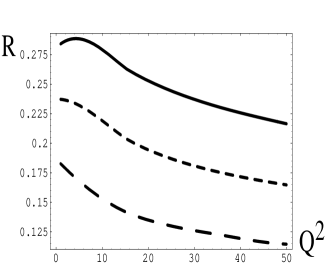
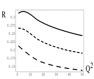
$\mathbf{A}$=200	$\mathbf{A}$=300

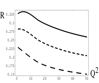
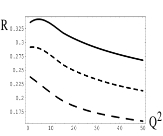
Figure 2: R as a function of the virtuality $Q^{2}$ for different $x$ and $A$. From the lower dashed curve to the solid one: $x=10^{-3}$, $x=10^{-4}$, $x=10^{-5}$ .

$\mathbf{Q^{2}\,\,=\,\,1\,GeV^{2}}$	$\mathbf{Q^{2}\,\,=\,\,5\,GeV^{2}}$
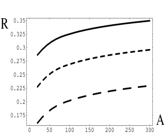
$\mathbf{Q^{2}\,\,=\,\,12\,GeV^{2}}$	$\mathbf{Q^{2}\,\,=\,\,30\,GeV^{2}}$
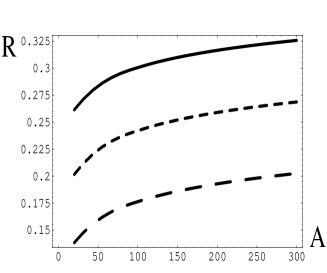
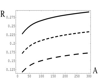
$\mathbf{Q^{2}\,\,=\,\,50\,GeV^{2}}$

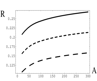
Figure 3: R as a function of the number of nucleons $A$ for different $x$ and $Q^{2}$. From the lower dashed curve to the solid one: $x=10^{-3}$, $x=10^{-4}$, $x=10^{-5}$..

Figure 4:R as a function of the virtuality $Q^{2}$	Figure 5: R as a function of number of
at $x=10^{-5}$. From the lower dashed	nucleons $A$ at $x=10^{-5}$. From the
curve to the solid one:	upper dashed curve to the solid one:
$A$ = 30, 100, 300.	$Q^{2}$ = 1, 5, 12, 30, 60 GeV2.

$\mathbf{Q^{2}\,\,=\,\,1\,GeV^{2}}$	$\mathbf{Q^{2}\,\,=\,\,12\,GeV^{2}}$
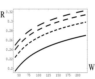
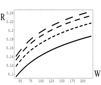
$\mathbf{Q^{2}\,\,=\,\,30\,GeV^{2}}$	$\mathbf{Q^{2}\,\,=\,\,60\,GeV^{2}}$

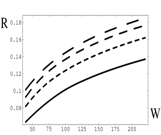
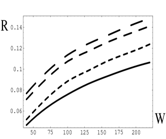
Figure 6: R as a function of the energy $W$ for different $A$ and $Q^{2}$. From the lower solid curve to the upper dashed one: $A$ = 30, 100, 200, 300.

$\mathbf{A=30\quad Q^{2}=12GeV^{2}}$	$\mathbf{A=200\quad Q^{2}=12GeV^{2}}$
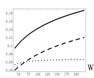
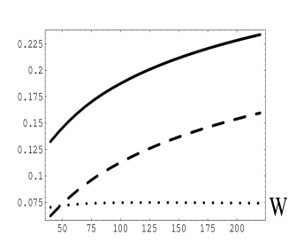
$\mathbf{A=30\quad Q^{2}=60GeV^{2}}$	$\mathbf{A=200\quad Q^{2}=60GeV^{2}}$

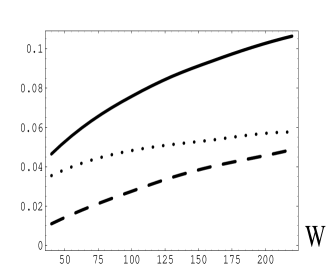
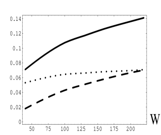
Figure 7: Different contributions to R as a function of the energy W for different $Q^{2}$ and A. Dashed line: contribution of the $q\bar{q}$ pair, dotted line: contribution of the $q\bar{q}G$ state, solid line - total contribution.

References

• [1] ZEUS collaboration: J. Breitweg et al., Eur. Phys. J. C6 (1999) 43;
H. Abramowicz and J.B. Dainton, J. Phys. G22 (1996) 911.
• [2] W. BuchmΓΌller, Towards the Theory of Diffractive DIS, DESY 99-076, hep-ph/9906546 and references therein.
• [3] K. Golec-Biernat and M. Wusthoff, Phys.Rev. D60 (1999) 114023; D59 (1999) 014017;
J.R. Forshaw, G. Kerley and G. Shaw, Phys.Rev. D60 (1999) 074012.
• [4] Yu. Kovchegov and L. McLerran, Phys.Rev. D60 (1999) 054025.
• [5] E. Gotsman, E. Levin and U. Maor, Nucl. Phys. B493 (1997) 354.
• [6] L.L. Frankfurt and M.I. Strikman, Phys. Lett. B382 (1996) 6.
• [7] A.H. Mueller, Nucl. Phys. B335 (1990) 115.
• [8] A.L. Ayala, M.B. Gay Ducati and E.M. Levin, Nucl. Phys. B493 (1997) 305; B510 (1998) 355.
• [9] Yu. V. Kovchegov, Phys. Rev. D60 (1999) 034008;,NUC-MN-99-8-T, May 1999. hep-ph/9905214;
E. Levin and K. Tuchin, DESY-99-108, Aug 1999. hep-ph/9908317.
• [10] L.V. Gribov, E.M. Levin and M.G. Ryskin, Phys. Rept. 100 (1983) 1.
• [11] A. Capella, A. Kaidalov and J. Tran Thanh Van, Heavy Ion Phys. 9 (1999) 169, hep-ph/9903244 and references therein.
• [12] E. Gotsman, E. Levin and U. Maor, Nucl.Phys .B464 (1996) 251.
• [13] E. Gotsman, E. Levin, M. Lublinsky, U. Maor and K. Tuchin, in preparation.
• [14] V.A. Abramovsky, V.N. Gribov and O.V. Kancheli, Sov. J. Nucl. Phys. 18 (1973) 308.
• [15] H.A. Enge, Introduction to nuclear physics, Addisson-Wesley, New York (1971).
• [16] A.L. Ayala, M.B. Gay Ducati and E.M. Levin, Phys. Lett. B388 (1996) 188.
• [17] M. GlΓΌck, E. Reya and A. Vogt, Z. Phys. C67 (1995) 433.
• [18] M. GlΓΌck, E. Reya and A. Vogt, Eur. Phys. J. C5 (1998) 461.
• [19] A.D. Martin, R.G. Roberts and W.J. Stirling, it Phys. Lett. B387 (1996) 419.
• [20] A.D. Martin, R.G. Roberts and W.J. Stirling, DTP-99-56, hep-ph/9906221.
• [21] CTEQ Collaboration: H.-L. Lai et al., Phys. Rev. D55 (1997) 1280 ; J.Huston et.al., hep-ph/9801444.