Theory of Nonleptonic $B$ Decays

Abstract:

I briefly review some recent progress in the theory of nonleptonic $B$ decays. After introducing the operator product expansion and the relevant effective Hamiltonian, I discuss the domain of validity and the theoretical justification of the factorization approximation and of its generalizations. Furthermore, I review some general parameterizations of $B$ decay amplitudes: the “diagrammatic” approach and the formalism based on Wick contractions in the matrix elements of four-fermion operators.

1 Introduction

The theoretical description of nonleptonic $B$ decays is an extremely difficult problem, due to the nonperturbative dynamics connected with hadronic final states. However, a good understanding of these transitions, or at least a reliable estimate of the theoretical uncertainties, is necessary to give a correct interpretation to the new data that are being collected at dedicated experiments. In particular, a meaningful test of the standard model and of its extensions on the most promising ground of CP violation in $B$ decays requires a good theoretical description of these processes.

The starting point of the analysis is the operator product expansion, that allows us to write the transition amplitude from a $B$ meson into a final state $F$ in terms of perturbative Wilson coefficients and nonperturbative hadronic matrix elements of local operators:

$$\mathcal{A}(B\to F)=\langle F|\mathcal{H}_{\mathrm{eff}}|B\rangle=$$

$$\frac{G_{F}}{\sqrt{2}}\sum_{i}V^{\mathrm{CKM}}_{i}C_{i}(\mu)\langle F|Q_{i}(\mu)|B\rangle,$$ (1)

where $\mu$ is the renormalization scale. The Wilson coefficients $C_{i}(\mu)$ and the matrix elements $\langle Q_{i}(\mu)\rangle$ are individually renormalization scale and scheme dependent, but they combine in eq. (1) to give a scale and scheme independent result for the amplitude (up to a residual scale dependence of higher order in the perturbative expansion). The $C_{i}(\mu)$ are universal, while all the dependence on the external states is carried by the matrix elements.

Wilson coefficients can be reliably computed in perturbation theory, and the full next-to-leading order results for $\mathcal{H}_{\mathrm{eff}}^{\Delta B=1}$ have been computed a few years ago by the Munich and Rome groups [1].

On the other hand, the computation of matrix elements requires the use of some nonperturbative technique. Unfortunately, a model independent computation of $\langle Q_{i}(\mu)\rangle$ from first principles on the lattice is not possible due to the Maiani-Testa no-go theorem [2]. A method to extract $\langle Q_{i}(\mu)\rangle$ from lattice QCD in a model-dependent way has been proposed [3], but its feasibility still has to be verified. Light-cone QCD sum rules might be used to estimate the matrix elements, however Final State Interaction (FSI) phases cannot be computed in this way [4]. It is therefore fair to say that at the moment no method is available to compute nonleptonic $B$ decays from first principles. One is then left with two possibilities.

The first is to use some approximation to simplify the dynamics to obtain an estimate of the matrix elements. Factorization is the simplest example of such approximations and it has been extensively used to study nonleptonic $B$ decays. The advantage of this kind of approach is the possibility of describing a large class of decay channels with few parameters. However, as we shall see in the following, factorization holds only in some channels and up to power-suppressed corrections. These corrections might, for example, play an important role in the extraction of CKM parameters from CP-violating $B$ decays. To estimate the possible effects of these power-suppressed terms, and to correctly describe those channels in which factorization cannot be justified, it is useful to develop another formalism. One can construct a general parameterization of weak decay amplitudes, including all possible hadronic dynamics. This can be supplemented with some symmetry argument to gain some predictive power, and when enough data are available, one can try to extract the hadronic parameters from the experiment.

In the following sections I will briefly summarize some recent progress that has been made in these two directions, discussing the advantages and disadvantages of these complementary approaches.

2 Factorization

The factorization approximation consists in writing the matrix element of a four-quark operator between the $B$ meson and a two-body hadronic final state as the product of two matrix elements of quark bilinears [5]–[7]. For example, let us consider the decay $\bar{B}^{0}\to D^{+}\pi^{-}$, which is mediated by the following operators:

$$Q_{1}=(\bar{d}u)_{V-A}(\bar{c}b)_{V-A},\;Q_{2}=(\bar{d}b)_{V-A}(\bar{c}u)_{V-A}.$$

In factorization, the matrix elements of $Q_{1}$ and $Q_{2}$ are written as

$$\langle\pi^{-}D^{+}|Q_{1}|\bar{B}^{0}\rangle_{\mathrm{F}}=\langle\pi^{-}|(\bar{d}u)_{A}|0\rangle\langle D^{+}|(\bar{c}b)_{V}|\bar{B}^{0}\rangle,$$

$$\langle\pi^{-}D^{+}|Q_{2}|\bar{B}^{0}\rangle_{\mathrm{F}}=\frac{1}{N}\langle\pi^{-}D^{+}|Q_{1}|\bar{B}^{0}\rangle_{\mathrm{F}}+$$

$$\frac{1}{2}\langle\pi^{-}D^{+}|(\bar{d}t^{a}u)_{V-A}(\bar{c}t^{a}b)_{V-A}|\bar{B}^{0}\rangle$$

$$\qquad\to\frac{1}{N}\langle\pi^{-}D^{+}|Q_{1}|\bar{B}^{0}\rangle_{\mathrm{F}},$$ (2)

where $t^{a}$ is a colour matrix, $N$ the number of colours and the octet-octet term in $\langle Q_{2}\rangle$ has been put to zero. From eq. (2) it is evident that in factorization final state interactions and gluon exchanges between the two currents are fully neglected. From eq. (2) one gets

$$\langle\pi^{-}D^{+}|\mathcal{H}_{\mathrm{eff}}|\bar{B}^{0}\rangle_{\mathrm{F}}\propto$$ (3)

$$\left(C_{1}(\mu)+\frac{1}{N}C_{2}(\mu)\right)\times\langle\pi^{-}D^{+}|Q_{1}|\bar{B}^{0}\rangle_{\mathrm{F}}.$$

The factorized matrix elements are then expressed in terms of form factors and decay constants. In this manner, the decay amplitudes can be computed as a function of the parameters [6]

$$a_{1}(\mu)\equiv C_{1}(\mu)+\frac{1}{N}C_{2}(\mu),$$ (4)

$$a_{2}(\mu)\equiv C_{2}(\mu)+\frac{1}{N}C_{1}(\mu).$$ (5)

Analogous parameters $a_{3}$–$a_{10}$ can be introduced for the contributions of QCD penguin operators $Q_{3-6}$ and electroweak penguin operators $Q_{7-10}$ (see ref. [1] for the definition of the basis of operators). Since $C_{2}$ is of $O(1/N)$ with respect to $C_{1}$, and has opposite sign, the two terms on the r.h.s. of eq. (5) tend to cancel each other, and therefore one finds that $a_{2}\ll a_{1}$. Channels governed by $a_{1}$ are usually called “colour allowed”, while transitions governed by $a_{2}$ are called “colour suppressed”. Care must however be taken when trying to quantify the effectiveness of colour suppression. Indeed, it strongly depends on the actual value of the Wilson coefficients and on the relative phase between the matrix elements of $Q_{1}$ and $Q_{2}$.

Factorization has been extensively used in phenomenological analyses of $B$ decays [6]–[8], and it has proven successful in estimating tree-dominated nonleptonic $B$ decays. However, from the theoretical point of view, it is clear that factorization cannot be exact. First of all, the factorized matrix element, being expressed in terms of form factors and decay constants, is scale- and scheme-independent, while the Wilson coefficients do depend on the renormalization scale and scheme. Therefore, eq. (3) shows that any decay amplitude computed with the factorization approximation carries these unphysical dependencies. Furthermore, the neglect of FSI phases and nonfactorizable contributions cannot in general be justified. Finally, it should also be stressed that the predictions within the factorization approach suffer from a considerable model dependence in the computation of the relevant form factors [9].

2.1 Generalized factorization

To overcome the problem of scale and scheme dependencies, two generalizations of the factorization approach have been proposed.

In the formulation of Neubert and Stech [10], the full matrix elements are split into the factorized expression plus a nonperturbative parameter $\varepsilon$:

$$\varepsilon^{(BD,\pi)}_{1}(\mu)\equiv\frac{\langle\pi^{-}D^{+}|(\bar{d}u)_{V-A}(\bar{c}b)_{V-A}|\bar{B}^{0}\rangle}{\langle\pi^{-}D^{+}|Q_{1}|\bar{B}^{0}\rangle_{\mathrm{F}}}-1,$$

$$\varepsilon^{(BD,\pi)}_{8}(\mu)\equiv\frac{\langle\pi^{-}D^{+}|(\bar{d}t^{a}u)_{V-A}(\bar{c}t^{a}b)_{V-A}|\bar{B}^{0}\rangle}{2\langle\pi^{-}D^{+}|Q_{1}|\bar{B}^{0}\rangle_{\mathrm{F}}}.$$

$\varepsilon_{1,8}(\mu)$ combine with $C_{1,2}(\mu)$ to give the scale and scheme independent parameters $a_{1}^{\mathrm{eff}}$ and $a_{2}^{\mathrm{eff}}$. In this framework there is no explicit calculation of non-factorizable contributions and $a_{1,2}^{\mathrm{eff}}$ are treated as free parameters to be extracted from the data.

In refs. [11]–[14], it has been proposed to improve on factorization by computing the $O(\alpha_{s})$ corrections to the matrix elements in perturbation theory:

$$\langle Q_{i}(\mu)\rangle\to g_{i}(\mu)\langle Q_{i}\rangle_{\mathrm{T}},$$ (6)

where $\langle Q_{i}\rangle_{\mathrm{T}}$ denotes the tree-level matrix element and $g_{i}(\mu)$ is a scheme and scale dependent function. Then factorization is applied to $\langle Q_{i}\rangle_{\mathrm{T}}$:

$$C_{i}(\mu)\langle Q_{i}(\mu)\rangle \to C_{i}(\mu)g_{i}(\mu)\langle Q_{i}\rangle_{\mathrm{T}}$$ (7)

$$\to C_{i}^{\mathrm{eff}}\langle Q_{i}\rangle_{\mathrm{F}}.$$

The scheme and scale dependence of $g_{i}(\mu)$ matches that of $C_{i}(\mu)$, so that the effective coefficients $C_{i}^{\mathrm{eff}}$ are scheme and scale independent. Unfortunately, this result is obtained at the price of losing control over finite terms in the effective coefficients. Indeed, the $C_{i}^{\mathrm{eff}}$ computed with this recipe depend on the choice of the gauge and of the external quark momenta used in the perturbative evaluation of $g_{i}(\mu)$ [15]. To obtain effective coefficients that do not carry these dependencies and to give a physical meaning to $g_{i}(\mu)$, a factorization theorem is necessary.

2.2 Factorization theorems

The first step towards a factorization theorem was given by Bjorken’s colour transparency argument [16]. Let us consider a decay of the $B$ meson in two light pseudoscalars, where two light quarks are emitted from the weak interaction vertex as a fast-traveling small-size colour-singlet object. In the heavy-quark limit, soft gluons cannot resolve this colour dipole and therefore soft gluon exchange between the two light mesons decouples at lowest order in $\Lambda_{\mathrm{QCD}}/m_{b}$.

Dugan and Grinstein [17] put forward a proof of factorization for $B$ decays into a heavy-light final state, in which the light meson is emitted. Unfortunately, their proof is based on the use of the so-called “large energy effective theory”, which is known to be unsuitable to describe exclusive processes, since it fails to consistently account for the hadronization of the emitted meson [18]. The large energy effective theory can only be used to prove factorization for semi-inclusive processes [19].

Politzer and Wise [20] have applied the Brodsky and Lepage formalism [21] to write a factorization formula for nonleptonic $b\to c$ transitions in which a light meson is emitted and the spectator quark is absorbed by the charmed meson. The expression, valid in the limit of heavy $b$ and $c$ quarks with $r=m_{c}/m_{b}$ fixed, reads:

$$\langle H_{c}(v^{\prime})\pi(P)|Q_{i}(m_{b})|H_{b}(v)\rangle=$$ (8)

$$\frac{1}{4}\langle H_{c}(v^{\prime})|\bar{h}_{v^{\prime}}^{(c)}h_{v}^{(b)}|H_{b}(v)\rangle m_{b}f_{\pi}(1-r)\times$$

$$\int_{0}^{1}\mathrm{d}x\,T_{i}^{\mathrm{(S)}}(x,r,m_{b})\phi_{\pi}(x,m_{b})+$$

$$\frac{1}{4}\langle H_{c}(v^{\prime})|\bar{h}_{v^{\prime}}^{(c)}\gamma_{5}h_{v}^{(b)}|H_{b}(v)\rangle m_{b}f_{\pi}(1+r)\times$$

$$\int_{0}^{1}\mathrm{d}x\,T_{i}^{\mathrm{(P)}}(x,r,m_{b})\phi_{\pi}(x,m_{b}),$$

where the renormalization scale has been set to $m_{b}$ and $\phi_{\pi}(x,m_{b})$ is the pion light-cone distribution amplitude. The hard scattering amplitudes $T_{i}^{\mathrm{(S,P)}}(x,r,m_{b})$ can be perturbatively expanded in $\alpha_{s}(m_{b})$ and are obtained from the computation of the diagrams in fig. 1.

Figure 1: Feynman diagrams for the computation of the hard scattering amplitudes $T$.

Beneke, Buchalla, Neubert and Sachrajda [22] have recently extended this formulation to $B$ decays into two light mesons and supplemented it with an explicit one-loop proof of factorization for $B\to\pi\pi$ decays valid in the limit of a heavy $B$ meson. Assuming that in $B\to\pi\pi$ decays perturbative Sudakov suppression is not sufficient to guarantee the dominance of hard spectator interactions, they argue that all soft spectator interactions can be absorbed in the $B\to\pi$ form factor. They therefore obtain the following factorization formula, valid at lowest order in $\Lambda_{\mathrm{QCD}}/m_{b}$:

$$\langle\pi(p^{\prime})\pi(q)|Q_{i}|\bar{B}(p)\rangle=$$ (9)

$$f^{B\to\pi}(q^{2})\int_{0}^{1}\mathrm{d}x\,T_{i}^{I}(x)\phi_{\pi}(x)+$$

$$\int_{0}^{1}\mathrm{d}\xi\,\mathrm{d}x\,\mathrm{d}y\,T^{II}_{i}(\xi,x,y)\phi_{B}(\xi)\phi_{\pi}(x)\phi_{\pi}(y),$$

where $f^{B\to\pi}(q^{2})$ is a $B\to\pi$ form factor, and $\phi_{\pi}$ $(\phi_{B})$ are leading-twist light cone distribution amplitudes of the pion ($B$ meson). Analogously to eq. (8), $T^{I,II}_{i}$ denote the hard scattering amplitudes. It is important to notice that $T^{I}$ starts at zeroth order in $\alpha_{s}$, giving factorization as in eq. (2), and at higher order contains hard gluon exchange not involving the spectator, while $T^{II}$ contains the hard interactions of the spectator and starts at order $\alpha_{s}$ (see fig. 2). This implies that factorization formulae for $B\to\pi\pi$ based on the dominance of hard spectator interactions [23, 24] miss the leading contribution in $\alpha_{s}$, unless Sudakov suppression is so effective that hard interactions of the spectator are dominant over soft ones. This controversial point should be clarified in order to determine the relative weight of the two terms on the r.h.s. in eq. (9).

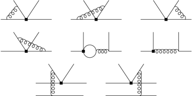
Figure 2: Order $\alpha_{s}$ corrections to the hard scattering kernels $T_{i}^{I}$ (first two rows) and $T_{i}^{II}$ (third row).

In the case where the spectator is absorbed by a heavy meson, the second term on the r.h.s. in eq. (9) is power suppressed (i.e. hard interactions of the spectator are power suppressed) and one recovers eq. (8). Finally, if a heavy meson is emitted, factorization cannot be justified.

The scheme and scale dependence of the scattering kernels $T^{I,II}_{i}$ matches the one of Wilson coefficients, and the final result is consistently scale and scheme independent.

Final state interaction phases appear in this formalism as imaginary parts of the scattering kernels (at lowest order in $\Lambda_{\mathrm{QCD}}/m_{b}$). These phases appear in the computation of penguin contractions and of hard gluon exchange between the two pions. This means that in the heavy quark limit final state interactions can be determined perturbatively.

The formalism of ref. [22] is certainly a very interesting theoretical result. From the point of view of phenomenological applications, however, the issue of $\Lambda_{\mathrm{QCD}}/m_{b}$ corrections is still an open problem that deserves further investigation, especially in those cases where $\Lambda_{\mathrm{QCD}}/m_{b}$ corrections are chirally or Cabibbo enhanced.

3 General Parameterizations

In order to identify possibly dangerous nonfactorizable contributions and to estimate the uncertainties in the extraction of standard model parameters from nonleptonic $B$ decays, it is useful to complement the above approach developing a general parameterization of decay amplitudes.

3.1 The “diagrammatic” approach

The diagrammatic approach [26, 27] has been extensively used to describe CP violating $B$ decays. It is based on the flavour-flow topologies of Feynman diagrams in the full theory.

In the approach of ref. [27] the basic parameters for strangeness preserving decays are the “Tree” (colour favoured) amplitude $T$, the “colour suppressed” amplitude $C$, the “penguin” amplitude $P$, the “exchange” amplitude $E$, the “annihilation” amplitude $A$ and the “penguin annihilation” amplitude ${\it PA}$. For strangeness changing decays one has $T^{\prime}$, $C^{\prime}$, $P^{\prime}$, $E^{\prime}$, $A^{\prime}$, ${\it PA}^{\prime}$. If $Z$-penguins are taken into account one introduces in addition the “colour-allowed” $Z$-penguin $P_{\scriptscriptstyle{\rm EW}}$ and the “colour-suppressed” $Z$-penguin $P^{C}_{\scriptscriptstyle{\rm EW}}$. Similarly $P_{\scriptscriptstyle{\rm EW}}^{\prime}$ and $P_{\scriptscriptstyle{\rm EW}}^{\prime C}$ are introduced for strangeness-changing decays.

Recently the usefulness of the diagrammatic approach has been questioned with respect to the effects of final state interactions. In particular various “plausible” diagrammatic arguments to neglect certain flavour-flow topologies may not hold in the presence of FSI, which mix up different classes of diagrams [28]–[35]. Another criticism which one may add is the lack of an explicit relation of this approach to the basic framework for non-leptonic decays represented by the effective weak Hamiltonian and OPE in eq. (1). In particular, the diagrammatic approach is governed by Feynman drawings with $W$-, $Z$- and top-quark exchanges. Yet such Feynman diagrams with full propagators of heavy fields represent really the situation at very short distance scales $O(M_{W,Z},m_{t})$, whereas the true picture of a decaying meson with a mass $O(m_{b})$ is more properly described by effective point-like vertices represented by the local operators $Q_{i}$. The effect of $W,Z$ and top quark exchanges is then described by the values of the Wilson coefficients of these operators. The only explicit fundamental degrees of freedom in the effective theory are the quarks $u$, $d$, $s$, $c$, $b$, the gluons and the photon.

In view of this situation it is desirable to develop another phenomenological approach based directly on the OPE which allows a systematic description of non-factorizable contributions such as penguin contributions and final state interactions. Simultaneously one would like to have an approach that does not lose the intuition of the diagrammatic approach while avoiding the limitations of the latter.

3.2 Wick contractions and charming penguins

A general parameterization which fulfills the above requirements has been proposed in ref. [35]. This approach is based on identifying the different topologies of Wick contractions in the matrix elements of the operators $Q_{i}$ (see figs. 3 and 4). There are emission topologies: Disconnected Emission (DE) and Connected Emission (CE); annihilation topologies: Disconnected Annihilation (DA) and Connected Annihilation (CA); emission annihilation topologies: Disconnected Emission Annihilation (DEA) and Connected Emission Annihilation (CEA); penguin topologies: Disconnected Penguin (DP) and Connected Penguin (CP); penguin emission topologies: Disconnected Penguin Emission (DPE) and Connected Penguin Emission (CPE); penguin annihilation topologies: Disconnected Penguin Annihilation (DPA) and Connected Penguin Annihilation (CPA); double penguin annihilation topologies: Disconnected Double Penguin Annihilation ($\overline{\it DPA}$) and Connected Double Penguin Annihilation ($\overline{\it CPA}$). The dashed lines represent the operators. All these parameters are flavour dependent, and some symmetry argument or dynamical assumption is needed in general to relate parameters entering different decay channels. The apparently disjoint pieces in the topologies DEA, CEA, DPE, CPE, DPA, CPA, $\overline{\it DPA}$ and $\overline{\it CPA}$ are connected to each other by gluons or photons, which are not explicitly shown. These special topologies in which only gluons connect the disjoint pieces are Zweig suppressed and are therefore naively expected to play a minor role in $B$ decays. However, they have to be included in order to define scheme and scale independent combinations of Wilson coefficients and matrix elements (see Section 3.3).

Figure 3: Emission and annihilation topologies of Wick contractions in the matrix elements of operators $Q_{i}$.

Figure 4: Penguin topologies of Wick contractions in the matrix elements of operators $Q_{i}$.

The Wick contractions are complex because of final state interactions. For example, it is easy to show that a disconnected emission followed by a rescattering is equivalent to a connected penguin. The same holds for annihilations. Therefore, by computing all possible Wick contractions one is automatically taking into account all rescattering effects in a consistent way.

The decay amplitude can be readily identified as a sum of Wilson coefficients times Wick contractions. These Wick contractions might eventually be computed on the lattice, with the caveat discussed in the Introduction. Letting the parameters vary in reasonable ranges, it is possible to obtain a reliable estimate of the uncertainties in the extraction of CKM parameters from CP asymmetries in $B$ decays.

It is interesting to note that some particular topologies, the so-called “charming penguins”, i.e. penguin contractions with a $c$-quark loop, can give very large contributions to some decay channels, even if their absolute value is very small. A typical example is given by $B\to K\pi$ decays [35, 36], where the following contributions are present (neglecting annihilations and GIM-suppressed penguins):

1. The contribution of emission matrix elements of current-current operators containing up quarks, which is doubly Cabibbo suppressed, but has Wilson coefficients and matrix elements of $O(1)$ (we normalize all matrix elements to DE for simplicity):

   $$V_{us}V_{ub}^{*}\left(C_{1}\langle Q_{1}^{u}\rangle_{\mathit{DE}}+C_{2}\langle Q_{2}^{u}\rangle_{\mathit{CE}}\right)$$

   $$\qquad\sim O(\lambda^{4}\cdot 1\cdot 1);$$ (10)

2. The contribution of emission matrix elements of penguin operators, which is Cabibbo allowed, but has Wilson coefficients of $O(10^{-2})$ and matrix elements of $O(1)$:

   $$V_{ts}V_{tb}^{*}\sum_{i=2}^{5}\left(C_{2i-1}\langle Q_{2i-1}\rangle_{\mathit{DE}}+C_{2i}\langle Q_{2i}\rangle_{\mathit{CE}}\right)$$

   $$\qquad\sim O(\lambda^{2}\cdot 10^{-2}\cdot 1);$$ (11)

3. The contribution of penguin contractions of current-current operators involving the charm quark (charming penguins), which is Cabibbo allowed, has Wilson coefficients of $O(1)$ and small ($O(\Lambda_{\mathrm{QCD}}/m_{b})$ in the framework of ref. [22]) matrix elements:

   $$V_{ts}V_{tb}^{*}\left(C_{1}\langle Q_{1}^{c}\rangle_{\mathit{DP}}+C_{2}\langle Q_{2}^{c}\rangle_{\mathit{CP}}\right)$$

   $$\qquad\sim O(\lambda^{2}\cdot 1\cdot\frac{\Lambda_{\mathrm{QCD}}}{m_{b}});$$ (12)

4. The contribution of penguin contractions of penguin operators, which is Cabibbo allowed but has small Wilson coefficients and matrix elements:

   $$V_{ts}V_{tb}^{*}\sum_{i=2}^{5}\left(C_{2i-1}\langle Q_{2i-1}\rangle_{\mathit{DP}}+C_{2i}\langle Q_{2i}\rangle_{\mathit{CP}}\right)$$

   $$\qquad\sim O(\lambda^{2}\cdot 10^{-2}\cdot\frac{\Lambda_{\mathrm{QCD}}}{m_{b}}).$$ (13)

It is evident that the contribution of charming penguins is likely to be large even for values of the penguin contractions of $O(\Lambda_{\mathrm{QCD}}/m_{b})$, thanks to the Cabibbo enhancement and the large Wilson coefficient. This means that great care should be taken in applying the factorization approach of ref. [22] to these channels, and particularly in estimating hadronic uncertainties in the extraction of the angle $\gamma$ from these decays [37, 38].

3.3 A RGE invariant parameterization

One disadvantage of the above formalism is that the Wick contraction parameters $DE$, $CE$ etc., individually depend on the renormalization scale and scheme and they combine in a rather complicated way with the Wilson coefficients to give a scheme and scale independent result. It is however possible to identify a complete set of scale and scheme independent parameters, made up of combinations of Wilson coefficients and Wick parameters [39]. This means that it is possible to give an expression for the decay amplitude that is manifestly RGE invariant and retains all the advantages of the effective Hamiltonian approach. There is a correspondence of these parameters with the parameters of the “diagrammatic” approach: in some sense, these RGE invariant parameters are the translation in the effective Hamiltonian language of the parameters of the diagrammatic approach.

I now briefly describe the RGE invariant effective parameters. The interested reader will find the complete definition of the effective parameters in ref. [39], together with a detailed derivation.

The first scale and scheme independent combinations of Wilson coefficients and matrix elements that one can identify correspond to the $T$ and $C$ parameters of the diagrammatic approach. Denoting by $\langle Q_{i}\rangle_{DE}$ and $\langle Q_{i}\rangle_{CE}$ the insertions of $Q_{i}$ into ${\it DE}$ and ${\it CE}$ topologies respectively, one finds two effective parameters

$$E_{1} = C_{1}\,\langle Q_{1}\rangle_{{\it DE}}+C_{2}\,\langle Q_{2}\rangle_{{\it CE}}\,,$$

$$E_{2} = C_{1}\,\langle Q_{1}\rangle_{{\it CE}}+C_{2}\,\langle Q_{2}\rangle_{{\it DE}}\,.$$ (14)

For simplicity, we suppress here and in the following the flavour variables. They are given explicitly in ref. [39]. $E_{1}$ and $E_{2}$ are generalizations of $a_{1}^{\rm eff}\langle Q_{1}\rangle_{F}$ and $a_{2}^{\rm eff}\langle Q_{2}\rangle_{F}$ in the formulation of ref. [10].

Next, annihilation topologies must be considered. The $A$ and $E$ parameters of the diagrammatic approach correspond respectively to the effective parameters

$$A_{1} = C_{1}\,\langle Q_{1}\rangle_{\it DA}+C_{2}\,\langle Q_{2}\rangle_{\it CA}\,,$$

$$A_{2} = C_{1}\,\langle Q_{1}\rangle_{\it CA}+C_{2}\,\langle Q_{2}\rangle_{\it DA}\,,$$ (15)

where $\langle Q_{i}\rangle_{\it DA}$ and $\langle Q_{i}\rangle_{\it CA}$ denote the $Q_{i}$-insertions into ${\it DA}$ and ${\it CA}$ topologies respectively. Due to the flavour structure of operators $Q_{1}$ and $Q_{2}$, $A_{1}$ can only contribute to $B^{+}$ decays while $A_{2}$ can only contribute to $B_{d,s}$ decays.

The last class of non-penguin contractions that we consider corresponds to the insertion of $Q_{1}$ and $Q_{2}$ into emission-annihilation topologies, denoted by ${\it DEA}$ and ${\it CEA}$ in fig. 3. Proceeding as above, we can identify two new effective parameters:

$${\it EA}_{1} = C_{1}\,\langle Q_{1}\rangle_{\it DEA}+C_{2}\,\langle Q_{2}\rangle_{\it CEA},$$

$${\it EA}_{2} = C_{1}\,\langle Q_{1}\rangle_{\it CEA}+C_{2}\,\langle Q_{2}\rangle_{\it DEA}.$$ (16)

As in the case of $A_{1}$ and $A_{2}$, due to the flavour structure of $Q_{1}$ and $Q_{2}$, ${\it EA}_{1}$ can only contribute to $B^{+}$ decays while ${\it EA}_{2}$ can only contribute to $B_{d,s}$ decays.

The situation with penguin contractions is a little bit more involved. Indeed, to obtain scale and scheme independent effective parameters it is necessary to combine penguin contractions of current-current operators and matrix elements of QCD and electroweak penguin operators.

Similarly to the sets $(E_{1},E_{2})$, $(A_{1},A_{2})$ and $({\it EA}_{1},{\it EA}_{2})$ one can find four effective “penguin”-parameters $P_{1}$, $P_{2}$, $P_{3}$ and $P_{4}$:

1. $P_{1}$ involves the insertions of $Q_{1}$ and $Q_{2}$ into ${\it CP}$ and ${\it DP}$ topologies respectively and a particular set of matrix elements of QCD-penguin and electroweak penguin operators necessary for the cancellation of scale and scheme dependences;

2. $P_{2}$ involves the insertions of $Q_{1}$ and $Q_{2}$ into ${\it CPE}$ and ${\it DPE}$ topologies respectively and a suitable set of matrix elements of QCD-penguin and electroweak penguin operators necessary for the cancellation of scale and scheme dependences;

3. $P_{3}$ involves the insertions of $Q_{1}$ and $Q_{2}$ into ${\it CPA}$ and ${\it DPA}$ topologies respectively and the corresponding set of matrix elements of QCD-penguin and electroweak penguin operators necessary for the cancellation of scale and scheme dependences;

4. $P_{4}$ involves the insertions of $Q_{1}$ and $Q_{2}$ into $\overline{\it CPA}$ and $\overline{\it DPA}$ topologies respectively and the remaining matrix elements of QCD-penguin and electroweak penguin operators which have not been included in $P_{1}$, $P_{2}$ and $P_{3}$.

The explicit expressions for the $P_{1}$, $P_{2}$, $P_{3}$ and $P_{4}$ parameters are as follows:

$$P_{1} = C_{1}\langle Q_{1}\rangle^{c}_{\it CP}+C_{2}\langle Q_{2}\rangle^{c}_{DP}$$

$$+ \sum_{i=2}^{5}\Bigl{(}C_{2i-1}\langle Q_{2i-1}\rangle_{{\it CE}}+C_{2i}\langle Q_{2i}\rangle_{{\it DE}}\Bigr{)}$$

$$+ \sum_{i=3}^{10}\Bigl{(}C_{i}\langle Q_{i}\rangle_{\it CP}+C_{i}\langle Q_{i}\rangle_{DP}\Bigr{)}$$

$$+ \sum_{i=2}^{5}\Bigl{(}C_{2i-1}\langle Q_{2i-1}\rangle_{\it CA}+C_{2i}\langle Q_{2i}\rangle_{\it DA}\Bigr{)}\,,$$

$$P_{2} = C_{1}\langle Q_{1}\rangle^{c}_{\it CPE}+C_{2}\langle Q_{2}\rangle^{c}_{\it DPE}$$

$$+ \sum_{i=2}^{5}\Bigl{(}C_{2i-1}\langle Q_{2i-1}\rangle_{{\it DE}}+C_{2i}\langle Q_{2i}\rangle_{{\it CE}}\Bigr{)}$$

$$+ \sum_{i=2}^{5}\Bigl{(}C_{2i-1}\langle Q_{2i-1}\rangle_{{\it CEA}}+C_{2i}\langle Q_{2i}\rangle_{{\it DEA}}\Bigr{)}$$

$$+ \sum_{i=3}^{10}\Bigl{(}C_{i}\langle Q_{i}\rangle_{\it CPE}+C_{i}\langle Q_{i}\rangle_{\it DPE}\Bigr{)}\,,$$

$$P_{3} = C_{1}\langle Q_{1}\rangle^{c}_{\it CPA}+C_{2}\langle Q_{2}\rangle^{c}_{\it DPA}$$

$$+ \sum_{i=2}^{5}\Bigl{(}C_{2i-1}\langle Q_{2i-1}\rangle_{\it DA}+C_{2i}\langle Q_{2i}\rangle_{\it CA}\Bigr{)}$$

$$+ \sum_{i=3}^{10}\Bigl{(}C_{i}\langle Q_{i}\rangle_{\it CPA}+C_{i}\langle Q_{i}\rangle_{\it DPA}\Bigr{)}\,,$$

$$P_{4} = C_{1}\langle Q_{1}\rangle^{c}_{\overline{\it CPA}}+C_{2}\langle Q_{2}\rangle^{c}_{\overline{\it DPA}}$$ (17)

$$+ \sum_{i=2}^{5}\Bigl{(}C_{2i-1}\langle Q_{2i-1}\rangle_{\it DEA}+C_{2i}\langle Q_{2i}\rangle_{\it CEA}\Bigr{)}$$

$$+ \sum_{i=3}^{10}\Bigl{(}C_{i}\langle Q_{i}\rangle_{\overline{\it CPA}}+C_{i}\langle Q_{i}\rangle_{\overline{\it DPA}}\Bigr{)}\,,$$

where we have denoted by $\langle Q_{i}\rangle^{c}_{\it CP}$ the insertion of operator $Q_{i}$ in a CP topology with a $c$-quark running in the loop (this corresponds to the charming penguin of ref. [35]), and analogously for ${\it DP}$, ${\it CPE}$, ${\it DPE}$, ${\it CPA}$, ${\it DPA}$, $\overline{\it CPA}$ and $\overline{\it DPA}$ topologies. Notice that, due to the flavour structure of the penguin-annihilation contributions, $P_{3}$ and $P_{4}$ cannot contribute to $B^{+}$ decays. Moreover $P_{4}$ contributes only to final states with two flavour neutral mesons $\bar{q}_{1}q_{1}$ and $\bar{q}_{2}q_{2}$. Similarly $P_{2}$ contributes only to states with at least one flavour neutral meson $\bar{q}_{2}q_{2}$.

The $P_{i}$ parameters are always accompanied by the CKM factor $V_{tb}V_{td_{i}}^{*}$, where $d_{i}={d,s}$. Penguin-type matrix elements are also present in the part of ${\cal H}_{\rm eff}$ proportional to $V_{ub}V_{ud_{i}}^{*}$. They correspond to penguin contractions of operators $Q_{1,2}$, or, more precisely, of the differences $\Bigl{(}Q_{1}^{d_{i}uu}-Q_{1}^{d_{i}cc}\Bigr{)}$ and $\Bigl{(}Q_{2}^{d_{i}uu}-Q_{2}^{d_{i}cc}\Bigr{)}$. When these combinations are inserted into penguin topologies, they give rise to a generalization of the GIM penguins of ref. [35]. The scale and scheme independent contributions are given by

$$P_{1}^{\scriptscriptstyle{\rm GIM}} = C_{1}\Bigl{(}\langle Q_{1}\rangle^{c}_{\it CP}-\langle Q_{1}\rangle^{u}_{\it CP}\Bigr{)}$$

$$+ C_{2}\Bigl{(}\langle Q_{2}\rangle^{c}_{DP}-\langle Q_{2}\rangle^{u}_{DP}\Bigr{)}\,,$$

$$P_{2}^{\scriptscriptstyle{\rm GIM}} = C_{1}\Bigl{(}\langle Q_{1}\rangle^{c}_{\it CPE}-\langle Q_{1}\rangle^{u}_{\it CPE}\Bigr{)}$$

$$+ C_{2}\Bigl{(}\langle Q_{2}\rangle^{c}_{\it DPE}-\langle Q_{2}\rangle^{u}_{\it DPE}\Bigr{)}\,,$$

$$P_{3}^{\scriptscriptstyle{\rm GIM}} = C_{1}\Bigl{(}\langle Q_{1}\rangle^{c}_{\it CPA}-\langle Q_{1}\rangle^{u}_{\it CPA}\Bigr{)}$$

$$+ C_{2}\Bigl{(}\langle Q_{2}\rangle^{c}_{\it DPA}-\langle Q_{2}\rangle^{u}_{\it DPA}\Bigr{)}\,,$$

$$P_{4}^{\scriptscriptstyle{\rm GIM}} = C_{1}\Bigl{(}\langle Q_{1}\rangle^{c}_{\overline{\it CPA}}-\langle Q_{1}\rangle^{u}_{\overline{\it CPA}}\Bigr{)}$$ (18)

$$+ C_{2}\Bigl{(}\langle Q_{2}\rangle^{c}_{\overline{\it DPA}}-\langle Q_{2}\rangle^{u}_{\overline{\it DPA}}\Bigr{)}\,,$$

and vanish in the limit of degenerate $u$ and $c$. The unitarity of the CKM matrix assures that in a given decay $P_{i}$ is always accompanied by $P_{i}^{\scriptscriptstyle{\rm GIM}}$. However, $P_{i}$ and $P_{i}^{\scriptscriptstyle{\rm GIM}}$ are always multiplied by different CKM factors and in order to study CP violation it is more convenient to keep the latter factors explicitly and consider separately $P_{i}$ and $P_{i}^{\scriptscriptstyle{\rm GIM}}$.

The relation to the parameters of the diagrammatic approach is the following:

$$P_{c}-P_{t}+P^{c}_{\scriptscriptstyle{\rm EW}}-P^{t}_{\scriptscriptstyle{\rm EW}} \leftrightarrow P_{1},$$

$$P_{c}-P_{u}+P^{c}_{\scriptscriptstyle{\rm EW}}-P^{u}_{\scriptscriptstyle{\rm EW}} \leftrightarrow P_{1}^{\scriptscriptstyle{\rm GIM}}\,.$$ (19)

A hierarchy between the effective parameters can be established with the help of some dynamical considerations. As an example, I report here the results of a large $N$ classification [39]. One has in units of $\sqrt{N}$ the following hierarchy for various topologies:

$${\it DE},\,{\it DA} : \,\,O(1),$$ (20)

$${\it CE},\,{\it CA},\,{\it DEA},\,{\it CP},\,{\it DPA},\,{\it DPE} : \,\,O(1/N),$$

$${\it CEA},\,{\it DP},\,{\it CPA},\,{\it CPE},\,{\it\overline{DPA}} : \,\,O(1/N^{2}),$$

$${\it\overline{CPA}} : \,\,O(1/N^{3}).$$

Combining these results with the large $N$ hierarchy of Wilson coefficients one gets the following classification of the effective parameters in units of $\sqrt{N}$:

$$E_{1},\,\,A_{1} : \,\,O(1),$$ (21)

$$E_{2},\,\,A_{2},\,\,{\it EA}_{1},\,\,P_{1},\,\,P_{1}^{\scriptscriptstyle{\rm GIM}} : \,\,O(1/N),$$

$${\it EA}_{2},\,\,P_{2},\,\,P_{3},\,\,P_{2}^{\scriptscriptstyle{\rm GIM}},\,\,P_{3}^{\scriptscriptstyle{\rm GIM}} : \,\,O(1/N^{2}),$$

$$P_{4},\,\,P_{4}^{\scriptscriptstyle{\rm GIM}} : \,\,O(1/N^{3}).$$

Using the above considerations, it is possible to divide two-body nonleptonic $B$ decay channels in various classes, according to the CKM structure and to the effective parameters entering the decay. This classification has been given in ref. [39], together with the full expressions of the decay amplitudes in terms of the effective parameters.

4 Conclusions and outlook

As I have summarized in the previous sections, some interesting progress has been recently made in our understanding of nonleptonic $B$ decays. Factorization in the limit of a heavy $B$ meson has been proven at one loop for $B$ decays to two light pseudoscalars [22], and it can be extended to decays to a heavy-light state where the spectator is absorbed by the heavy meson. At the lowest order in $\Lambda_{\mathrm{QCD}}/m_{b}$ corrections to the factorization approximation can be systematically computed in perturbation theory. In the same approximation, FSI can be computed perturbatively. These theoretically very exciting results should be confronted with phenomenology keeping in mind that nonfactorizable power corrections can in some cases be chirally or Cabibbo enhanced.

To this aim, general parameterizations of decay amplitudes can be very helpful in identifying the potentially dangerous contributions. For example, the Wick contraction parameterization of ref. [35], tightly connected to the OPE formalism, shows that a particular class of contributions, the “charming penguins” (penguin contractions of charmed current-current operators), can give large, if not dominant, contribution to many interesting decay channels such as $B\to K\pi$.

In its RGE invariant formulation [39], the Wick contraction parameterization benefits of the advantages of being directly connected to the effective Hamiltonian formalism, while maintaining the appealing simplicity of the diagrammatic approach.

It is very exciting to think that benefiting of these complementary approaches as well as of the wealth of forthcoming data we might be able in the near future to reach a good understanding of nonleptonic $B$ decays.