SUPERSYMMETRIC GRAND UNIFICATION : AN UPDATE
Lectures at Trieste Summer School, 1999

Abstract

Supersymmetry is believed to be an essential ingredient of physics beyond the standard model for several reasons. The foremost among them is its milder divergence structure which explains why the electroweak scale (or the Higgs mass) is stable under radiative corrections. Two other reasons adding to this belief are : (i) a way to understand the origin of the electroweak symmetry breaking as a consequence of radiative corrections and (ii) the particle content of the minimal supersymmetric model that leads in a natural way to the unification of the three gauge couplings of the standard model at a high scale. The last observation though not as compelling as the first two, however suggests, if taken seriously, that at scales close to the Planck scale, all matter and all forces may unify into a single matter and a single force leading to a supersymmetric grand unified theory. It is the purpose of these lectures to provide a pedagogical discussion of the various kinds of supersymmetric unified theories beyond the minimal supersymmetric standard model (MSSM) including SUSY GUTs and present a brief overview of their implications. Questions such as proton decay, R-parity violation, doublet triplet splitting etc. are discussed. Exhaustive discussion of $SU(5)$ and $SO(10)$ models and less detailed ones for other GUT models such as those based on $E_{6}$, $SU(5)\times SU(5)$, flipped SU(5) and $SU(6)$ are presented. Finally, an overview of the recent developements in theories with extra dimensions and their implications for the grand unified models is presented.

Table of contents

I: Introduction

1.1 Brief introduction to supersymmetric field theories

1.2 The minimal supersymmetric standard model (MSSM)

1.3 Why go beyond the MSSM ?

1.4 Origin of supersymmetry breaking: gravity mediated, gauge mediated, U(1) and conformal anomaly mediated models

1.5 Supersymmetric left-right models

1.6 Mass scales

II : Unification of couplings

2.1 Unification of gauge couplings (UGC)

2.2 UGC with intermediate scales

2.3 Yukawa unification and $m_{b},m_{\tau}$ and $m_{t}$

2.4 Mass scales in the light of grand unification

III. Supersymmetric SU(5)

3.1 Fermion and Higgs assignment, symmetry breaking

3.2 Low energy spectrum and doublet-triplet splitting

3.3 Fermion masses and Proton decay

3.4 Other implications of SU(5)

3.5 Problems and prospects

IV: Left-right symmetric GUT: The SO(10) example

4.1 Group theory of SO(10)

4.2 Symmetry breaking and fermion masses

4.3 Neutrino masses and R-parity breaking

4.4 Doublet-triplet splitting

4.5 Final comments

V: Beyond simple SUSY GUT’s- four examples

5.1 $E_{6}$

5.2 $SU(5)\times SU(5)$

5.3 $SU(5)\times U(1)$

5.4 $SU(6)$ and new approach to doublet-triplet splitting

5.5 $\mu\rightarrow e+\gamma$ as a test of certain grand unification models

5.5 Overall perspective

VI. String Theories, Extra Dimensions and Grand unification

6.1 Basic ideas of string theories

6.2 Heterotic string, gauge coupling unification and mass scales

6.3 Spectrum constraints

6.4 Strongly coupled strings, large extra dimensions and low string string scales

6.5 Effect of extra dimensions on gauge coupling unifications

1 Introduction

Supersymmetry, the symmetry between the bosons and fermions is one of the fundamental new symmetries of nature that has been the subject of intense discussion in particle physics of the past two decades. It was introduced in the early 1970’s by Golfand, Likhtman, Akulov, Volkov, Wess and Zumino (and in the context of two dimensional string world sheet by Gervais and Sakita). In addition to the obvious fact that it provides the hope of an unified understanding of the two known forms of matter, the bosons and fermions, it has also provided a mechanism to solve two conceptual problems of the standard model, viz. the possible origin of the weak scale as well as its stability under quantum corrections. Another attractive feature of supersymmetry is that when made a local symmetry it naturally leads to gravity as a part of unified theories. Furthermore the recent developments in strings, which embody supersymmetry in an essential way also promise the fulfilment of the eternal dream of all physicists to find an ultimate theory of everything. It would thus appear that there exist a large body of compelling theoretical arguments that have convinced contemporary particle physicists to accept that the theory of particles and forces must incorporate supersymmetry. Ultimate test of these ideas will of course come from the experimental discovery of the superpartners of the standard model particles with masses under a TeV and the standard model Higgs boson with mass less than about $130$ GeV.

Since supersymmetry transforms a boson to a fermion and vice versa, an irreducible representation of supersymmetry will contain in it both fermions and bosons. Therefore in a supersymmetric theory, all known particles are accompanied by a superpartner which is a fermion if the known particle is a boson and vice versa. For instance, the electron ($e$) supermultiplet will contain its superpartner $\widetilde{e}$, (called the selectron) which has spin zero. We will adopt the notation that the superpartner of a particle will be denoted by the same symbol as the particle with a ‘tilde’ as above. Furthermore, while supersymmetry does not commute with the Lorentz transformations, it commutes with all internal symmetries; as a result, all non-Lorentzian quantum numbers for both the fermion and boson in the same supermultiplet are the same. As in the case of all symmetries realized in the Wigner-Weyl mode, in the limit of exact supersymmetry, all particles in the same supermultiplet will have the same mass. Since this is contrary to what is observed in nature, supersymmetry has to be a broken symmetry. An interesting feature of supersymmetric theories is that the supersymmetry breaking terms are fixed by the requirement that the mild divergence structure of the theory remains uneffected. One then has a complete guide book for writing the local field theories with broken supersymmetry. We will not discuss the detailed introductory aspects of supersymmetry that are needed to write the Lagrangian for these models and instead refer to books and review articles on the subject[1, 2, 3, 4]. Let us however give the bare outlines of how one goes about writing the action for such models.

1.1 Brief introduction to the supersymmetric field theories

In order to write down the action for a supersymmetric field theory, let us start by considering generic chiral fields denoted by $\Phi(x,\theta)$ with component fields given by $(\phi,\psi)$ and gauge fields denoted by $V(x,\theta,\bar{\theta})$ with component gauge and gaugino fields given by $(A^{\mu},\lambda)$. The action in the superfield notation is

$$S=\int d^{4}x\int d^{2}\theta d^{2}{\bar{\theta}}\Phi^{\dagger}e^{V}\Phi+\int d^{4}x\int d^{2}\theta\left(W(\Phi)+W_{\lambda}(V)W_{\lambda}(V)\right)+h.c.$$ (1)

In the above equation, the first term gives the gauge invariant kinetic energy term for the matter fields $\Phi$; $W(\Phi)$ is a holomorphic function of $\Phi$ and is called the superpotential; it leads to the Higgs potential of the usual gauge field theories. Secondly, $W_{\lambda}(V)\equiv{\cal D}^{2}\bar{{\cal D}}V$ where ${\cal D}\equiv\partial_{\theta}-i\sigma.\partial_{x}$, and the term involving $W_{\lambda}(V)$ leads to the gauge invariant kinetic energy term for the gauge fields as well as for the gaugino fields. In terms of the component fields the lagrangian can be written as

$${\cal L}={\cal L}_{g}+{\cal L}_{matter}+{\cal L}_{Y}-V(\phi)$$ (2)

where

$${\cal L}_{g}=-\frac{1}{4}F^{\mu\nu}F_{\mu\nu}+\frac{1}{2}\bar{\lambda}\gamma^{\mu}iD_{\mu}\lambda$$

$${\cal L}_{matter}=|D_{\mu}\phi|^{2}+\bar{\psi}\gamma^{\mu}iD_{\mu}\psi$$

$${\cal L}_{V}=\sqrt{2}g\bar{\lambda}\psi\phi^{\dagger}+\psi_{a}\psi_{b}W_{ab}$$

$$V(\phi)=|W_{a}|^{2}+\frac{1}{2}{\cal D}_{\alpha}{\cal D}_{\alpha}$$ (3)

where $D_{\mu}$ stands for the covariant derivative with respect to the gauge group and ${\cal D}_{\alpha}$ stands for the so-called ${\cal D}$-term and is given by ${\cal D}_{\alpha}=g\phi^{\dagger}T_{\alpha}\phi$ ($g$ is the gauge coupling constant and $T_{\alpha}$ are the generators of the gauge group). $W_{a}$ and $W_{ab}$ are the first and second derivative of the superpotential $W$ with respect to the superfield with respect to the field $\Phi_{a}$, where the index $a$ stands for different matter fields in the model.

A very important property of supersymmetric field theories is their ultraviolet behavior which have the extremely important consequence that in the exact supersymmetric limit, the parameters of the superpotential $W(\Phi)$ do not receive any (finite or infinite) correction from Feynman diagrams involving the loops. In other words, if the value of a superpotential parameter is fixed at the classical level, it remains unchanged to all orders in perturbation theory. This is known as the non-renormalization theorem [5].

This observation was realized as the key to solving the Higgs mass problem of the standard model as follows: the radiative corrections to the Higgs mass in the standard model are quadratically divergent and admit the Planck scale as a natural cutoff if there is no new physics upto that level. Since the Higgs mass is directly proportional to the mass of the $W$-boson, the loop corrections would push the $W$-boson mass to the Planck scale destabilizing the standard model. On the other hand in the supersymmetric version of the standard model (to be called MSSM), in the limit of exact supersymmetry, there are no radiative corrections to any mass parameter and therefore to the Higgs boson mass which can therefore be set once and for all at the tree level. Thus if the world could be supersymmetric at all energy scales, the weak scale stability problem would be easily solved. However, since supersymmetry must be a broken symmetry, one has to ensure that the terms in the Hamiltonian that break supersymmetry do not spoil the non-renormalization theorem in a way that infinities creep into the self mass corrections to the Higgs boson. This is precisely what happens if effective supersymmetry breaking terms are “soft” which means that they are of the following type:

1. $m^{2}_{a}\phi^{\dagger}_{a}\phi_{a}$, where $\phi$ is the bosonic component of the chiral superfield $\Phi_{a}$;

2. $m\int d^{2}\theta\theta^{2}\left(AW^{(3)}(\Phi)+BW^{(2)}(\Phi)\right)$, where $W^{(3)}(\Phi)$ and $W^{(2)}(\Phi)$ are the second and third order polynomials in the superpotential.

3. $\frac{1}{2}m_{\lambda}\lambda^{T}C^{-1}\lambda$, where $\lambda$ is the gaugino field.

It can be shown that the soft breaking terms only introduce finite loop corrections to the parameters of the superpotential. Since all the soft breaking terms require couplings with positive mass dimension, the loop corrections to the Higgs mass will depend on these masses and we must keep them less than a TeV so that the weak scale remains stabilized. This has the interesting implication that superpartners of the known particles are accessible to the ongoing and proposed collider experiments. For a recent survey of the experimental situation, see Ref. [6, 7, 8].

The mass dimensions associated with the soft breaking terms depend on the particular way in which supersymmetry is broken. It is usually assumed that supersymmetry is broken in a sector that involves fields which do not have any quantum numbers under the standard model group. This is called the hidden sector. The supersymmetry breaking is then transmitted to the visible sector either via the gravitational interactions [9] or via the gauge interactions of the standard model [10] or via anomalous U(1) ${\cal D}$-terms [11]. In sec. 1.4, we discuss these different ways to break supersymmetry and their implications.

1.2 The minimal supersymmetric standard model (MSSM)

Let us now apply the discussions of the previous section to constuct the supersymmetric extension of the standard model so that the goal of stabilizing the Higgs mass is indeed realized in practice. The superfields and their representation content are given in Table I.

Table 1: The particle content of the supersymmetric standard model. For matter and Higgs fields, we have shown the left-chiral fields only. The right-chiral fields will have a conjugate representation under the gauge group.

Superfield	gauge transformation
Quarks $Q$	$(3,2,{1\over 3})$
Antiquarks $u^{c}$	$(3^{*},1,-{4\over 3})$
Antiquarks $d^{c}$	$(3^{*},1,\frac{2}{3})$
Leptons $L$	$(1,2-1)$
Antileptons $e^{c}$	$(1,1,+2)$
Higgs Boson $\bf H_{u}$	$(1,2,+1)$
Higgs Boson $\bf H_{d}$	$(1,2,-1)$
Color Gauge Fields $G_{a}$	$(8,1,0)$
Weak Gauge Fields $W^{\pm}$, $Z$, $\gamma$	$(1,3+1,0)$

First note that an important difference between the standard model and its supersymmetric version apart from the presence of the superpartners is the presence of a second Higgs doublet. This is required both to give masses to quarks and leptons as well as to make the model anomaly free. The gauge interaction part of the model is easily written down following the rules laid out in the previous section. In the weak eigenstate basis, weak interaction Lagrangian for the quarks and leptons is exactly the same as in the standard model. As far as the weak interactions of the squarks and the sleptons are concerned, the generation mixing angles are very different from those in the corresponding fermion sector due to supersymmetry breaking. This has the phenomenological implication that the gaugino-fermion-sfermion interaction changes generation leading to potentially large flavor changing neutral current effects such as $K^{0}$-$\bar{K}^{0}$ mixing, $\mu\to e\gamma$ decay etc unless the sfermion masses of different generations are chosen to be very close in mass.

Let us now proceed to a discussion of the superpotential of the model. It consists of two parts:

$$W=W_{1}+W_{2}\,,$$ (4)

where

$$W_{1}=h^{ij}_{\ell}e^{c}_{i}L_{j}{\bf H_{d}}+h^{ij}_{d}Q_{i}d^{c}_{j}{\bf H_{d}}+h^{ij}_{u}Q_{i}u^{c}_{j}{\bf H_{u}}+\mu{\bf H_{u}H_{d}}$$ (5)

$$W_{2}=\lambda_{ijk}L_{i}L_{j}e^{c}_{k}+\lambda^{\prime}_{ijk}L_{i}Q_{j}d^{c}_{k}+\lambda^{\prime\prime}_{ijk}u^{c}_{i}d^{c}_{j}d^{c}_{k}$$ (6)

$i,j,k$ being generation indices. We first note that the terms in $W_{1}$ conserve baryon and lepton number whereas those in $W_{2}$ do not. The latter are known as the $R$-parity breaking terms where $R$-parity is defined as

$$R=(-1)^{3(B-L)+2S}\,,$$ (7)

where $B$ and $L$ are the baryon and lepton numbers and $S$ is the spin of the particle. It is interesting to note that the $R$-parity symmetry defined above assigns even $R$-parity to known particles of the standard model and odd $R$-parity to their superpartners. This has the important experimental implication that for theories that conserve $R$-parity, the super-partners of the particles of the standard model must always be produced in pairs and the lightest superpartner must be a stable particle. This is generally called the LSP. If the LSP turns out to be neutral, it can be thought of as the dark matter particle of the universe.

We now assume that some kind of supersymmetry breaking mechanism introduces splitting for the squarks and sleptons from the quarks and the leptons. Usually, supersymmetry breaking can be expected to introduce trilinear scalar interactions amomg the sfermions as follows:

$${\cal L}^{SB}=m_{3/2}[A_{e,ab}\widetilde{e^{c}}_{a}\widetilde{L}_{b}H_{d}+A_{d,ab}\widetilde{Q}_{a}H_{d}\widetilde{d^{c}}_{b}+A_{u,ab}\widetilde{Q}_{a}H_{u}\widetilde{u^{c}}_{b}]$$ (8)

$$+B\mu m_{3/2}H_{u}H_{d}+\Sigma_{i={\rm scalars}}\mu^{2}_{i}\phi^{\dagger}_{i}\phi_{i}+\Sigma_{a}\frac{1}{2}M_{a}\lambda^{T}C^{-1}\lambda_{a}$$

There will also be the corresponding terms involving the $R$-parity breaking, which we omit here for simplicity.

As already announced this model solves the Higgs mass problem in the sense that if its tree level value is chosen to be of the order of the electroweak scale, any radiative correction to it will only induce terms of order $\sim\frac{f^{2}}{16\pi^{2}}M^{2}_{SUSY}$. By choosing the supersymmetry breaking scale in the TeV range, we can guarantee that to all orders in perturbation theory the Higgs mass remains stable.

Constraints of supersymmetry breaking provide one prediction that can distinguish it from the nonsupersymmetric models- i.e. the mass of the lightest Higgs boson. It can be shown that the lightest higgs boson mass-square is going to be of order $\sim g^{2}v^{2}_{wk}$ (Ref.[7]). In fact denoting the vev’s of the two Higgs doublets as $<H^{0}_{u}>=v_{u}$ and $<H^{0}_{d}>=v_{d}$, one can write:

$$m^{2}_{h}\simeq\frac{g^{2}+g^{\prime 2}}{4}(v^{2}_{d}-v^{2}_{u})$$ (9)

Defining $v_{u}/v_{d}=tan\beta$, we can rewrite the above light Higgs mass formula as $m^{2}_{h}=M^{2}_{Z}cos2\beta$ which implies that the tree level mass of the lightest Higgs boson is less than the $Z$ mass. Once radiative corrections are taken into account[7], $m_{h}$ increases above the $M_{Z}$. However, it is now well established that in a large class of supersymmetric models (which do not differ too much from the MSSM), the Higgs mass is less than 150 GeV or so.

Another very interesting property of the MSSM is that electroweak symmetry breaking can be induced by radiative corrections. As we will see below, in all the schemes for generating soft supersymmetry breaking terms via a hidden sector, one generally gets positive (mass)²’s for all scalar fields at the scale of SUSY breaking as well as equal mass-squares. In order to study the theory at the weak scale, one must extrapolate all these parameters using the renormalization group equations. The degree of extrapolation will of course depend on the strength of the gauge and the Yukawa couplings of the various fields. In particular, the $m^{2}_{H_{u}}$ will have a strong extrapolation proportional to $\frac{h^{2}_{t}}{16\pi^{2}}$ since $H_{u}$ couples to the top quark. Since $h_{t}\simeq 1$, this can make $m^{2}_{H_{u}}(M_{Z})<0$, leading to spontaneous breakdown of the electroweak symmetry. An approximate solution of the renormalization group equations gives

$$m^{2}_{H_{u}}(M_{Z})=m^{2}_{H_{u}}(\Lambda_{SUSY})-\frac{3h^{2}_{t}m^{2}_{\tilde{t}}}{16\pi^{2}}ln\frac{\Lambda^{2}_{SUSY}}{M^{2}_{Z}}$$ (10)

This is a very attractive feature of supersymmetric theories.

1.3 Why go beyond the MSSM ?

Even though the MSSM solves two outstanding peoblems of the standard model, i.e. the stabilization of the Higgs mass and the breaking of the electroweak symmetry, it brings in a lot of undesirable consequences. They are:

(a) Presence of arbitrary baryon and lepton number violating couplings i.e. the $\lambda$, $\lambda^{\prime}$ and $\lambda^{\prime\prime}$ couplings described above. In fact a combination of $\lambda^{\prime}$ and $\lambda^{\prime\prime}$ couplings lead to proton decay. Present lower limits on the proton lifetime then imply that $\lambda^{\prime}\lambda^{\prime\prime}\leq 10{-25}$ for squark masses of order of a TeV. Recall that a very attractive feature of the standard model is the automatic conservation of baryon and lepton number. The presence of R-parity breaking terms[15] also makes it impossible to use the LSP as the Cold Dark Matter of the universe since it is not stable and will therefore decay away in the very early moments of the universe. We will see that as we proceed to discuss the various grand unified theories, keeping the R-parity violating terms under control will provide a major constraint on model building.

(b) The different mixing matrices in the quark and squark sector leads to arbitrary amount of flavor violation manifesting in such phenomena as $K_{L}-K_{S}$ mass difference etc. Using present experimental information and the fact that the standard model more or less accounts for the observed magnitude of these processes implies that there must be strong constraints on the mass splittings among squarks. Detailed calculations indicate[16] that one must have $\Delta m^{2}_{\tilde{q}}/m^{2}_{\tilde{q}}\leq 10^{-3}$ or so. Again recall that this undoes another nice feature of the standard model.

(c) The presence of new couplings involving the super partners allows for the existence of extra CP phases. In particular the presence of the phase in the gluino mass leads to a large electric dipole moment of the neutron unless this phase is assumed to be suppressed by two to three orders of magnitude[17]. This is generally referred to in the literature as the SUSY CP problem. In addition, there is of course the famous strong CP problem which neither the standard model nor the MSSM provide a solution to.

In order to cure these problems as well as to understand the origin of the soft SUSY breaking terms, one must seek new physics beyond the MSSM. Below, we pursue two kinds of directions for new physics: one which analyses schemes that generate soft breaking terms and a second one which leads to automatic B and L conservation as well as solves the SUSY CP problem. The second model also provides a solution to the strong CP problem without the need for an axion under certain circumstances.

1.4 Mechanisms for supersymmetry breaking

One of the major focus of research in supersymmetry is to understand the mechanism for supersymmetry breaking. The usual strategy employed is to assume that SUSY is broken in a hidden sector that does not involve any of the matter or forces of the standard model (or the visible sector) and this SUSY breaking is transmitted to the visible sector via some intermediary , to be called the messenger sector.

There are generally two ways to set up the hidden sector- a less ambitious one where one writes an effective Lagrangian (or superpotential) in terms of a certain set of hidden sector fields that lead to supersymmetry breaking in the ground state and another more ambitious one where the SUSY breaking arises from the dynamics of the hidden sector interactions. For our purpose we will use the simpler schemes of the first kind. As far as the messenger sector goes there are three possibilities as already referred to earlier: (i) gravity mediated [9]; (ii) gauge mediated [10] and (iii) anomalous U(1) mediated[11]. Below we give examples of each class.

(i) Gravity mediated SUSY breaking

The scenario that uses gravity to transmit the supersymmetry breaking is one of the earliest hidden sector scenarios for SUSY breaking and forms much of the basis for the discussion in current supersymmetry phenomenology. In order to discuss these models one needs to know the supergravity couplings to matter. This is given in the classic paper of Cremmer et al.[18]. An essential feature of supergravity coupling is the generalized kinetic energy term in gravity coupled theories called the Kahler potential, $K$. We will denote this by $G$ and it is a hermitean operator which is a function of the matter fields in the theory and their complex conjugates. The effect of supergravity coupling in the matter and the gauge sector of the theory is given in terms of $G$ and its derivatives as follows:

$$L(z)=G_{zz^{*}}|\partial_{\mu}z|^{2}+e^{-G}[G_{z}G_{z^{*}}G^{-1}_{zz^{*}}+3]$$ (11)

where $z$ is the bosonic component of a typical chiral field (e.g. we would have $z\equiv\tilde{q},\tilde{l}$ etc) and $G=~{}3ln(\frac{-K}{3})-ln|W(z)|^{2}$. A superscript implies derivative with respect to that field. The simplest choice for the Kahler potential $K$ is $K=-3e^{-\frac{|z|^{2}}{3M^{2}_{P\ell}}}$ that normalizes the kinetic energy term properly. Using this, one can write the effective potential for supergravity coupled theories to be:

$$V(z,z^{*})=e^{\frac{|z|^{2}}{M^{2}_{P\ell}}}[|W_{z}+\frac{z^{*}}{M^{2}_{P\ell}}W|^{2}-\frac{3}{M^{2}_{P\ell}}|W|^{2}]+D-terms$$ (12)

The gravitino mass is given in terms of the Kahler potential as :

$$m_{3/2}=M_{P\ell}e^{-G/2}$$ (13)

A popular scenario suggested by Polonyi is based upon the following hidden sector consisting of a gauge singlet field, denoted by $z$ and the superpotential $W_{H}$ given by:

$$W_{H}=\mu^{2}(z+\beta)$$ (14)

where $\mu$ and $\beta$ are mass parameters to be fixed by various physical considerations. It is clear that this superpotential leads to an F-term that is always non-vanishing and therefore breaks supersymmetry. Requiring the cosmological constant to vanish fixes $\beta=(2-\sqrt{3})M_{Pl}$. Given this potential and the choice of the Kahler potential as discussed earlier, supergravity calculus predicts universal soft breaking parameters $m$ given by $m_{0}\sim\mu^{2}/M_{Pl}$. Requiring $m_{0}$ to be in the TeV range implies that $\mu\sim 10^{11}$ GeV. The complete potential to zeroth order in $M^{-1}_{P\ell}$ in this model is given by:

$$V(\phi_{a})=[\Sigma_{a}|\frac{\partial W}{\partial\phi_{a}}|^{2}+V_{D}]$$ (15)

$$+[m^{2}_{0}\Sigma_{a}\phi^{*}_{a}\phi_{a}+(AW^{(3)}+BW^{(2)}+h.c.)$$

where $W^{(3,2)}$ denote the dimension three and two terms in the superpotential respectively. The values of the parameters $A$ and $B$ at $M_{Pl}$ are related to each other in this example as $B=A-1$. The gaugino masses in these models arise out of a separate term in the Lagrangian depending on a new function of the hidden sector singlet fields, $z$:

$$\int d^{4}xd^{2}\theta f(z)W^{\alpha}_{\lambda}W_{\lambda,\alpha}$$ (16)

If we choose $f(z)=\frac{z}{M_{P\ell}}$, then gaugino masses come out to be of order $m_{3/2}\sim\frac{\mu^{2}}{M_{P\ell}}$ which is also of order $m_{0}$ , i.e. the electroweak scale. Furthermore, in order to avoid undesirable color and electric charge breaking by the SUSY models, one must require that $m^{2}_{0}\geq 0$.

It is important to point out that the superHiggs mechanism operates at the Planck scale. Therefore all parameters derived at the tree level of this model need to be extrapolated to the electroweak scale. So after the soft-breaking Lagrangian is extrapolated to the weak scale, it will look like:

$${\cal L}^{SB}=m^{2}_{a}\phi^{*}_{a}\phi_{a}+m\Sigma_{i,j,k}A_{ijk}\phi_{i}\phi_{j}\phi_{k}+\Sigma_{i,j}B_{ij}\phi_{i}\phi_{j}$$ (17)

These extrapolations depend among other things on the Yukawa couplings of the model. As a result of this the universality of the various SUSY breaking terms is no more apparent at the electroweak scale. Moreover, since the top Yukawa coupling is now known to be of order one, its effect turns the mass-squared of the $H_{u}$ negative at the electroweak scale even starting from a positive value at the Planck scale [19]. This provides a natural mechanism for the breaking of electrweak symmetry adding to the attractiveness of supersymmetric models. In the lowest order approximation, one gets,

$$m^{2}_{H_{u}}(M_{Z})\sim m^{2}_{H_{u}}(M_{P\ell})-\frac{3h^{2}_{t}}{8\pi^{2}}ln(\frac{M_{P\ell}}{M_{Z}})(m^{2}_{H_{u}}+m^{2}_{\tilde{q}}+m^{2}_{u^{c}})|_{\mu=M_{P\ell}}$$ (18)

Fig. 1 depicts the actual evolution of the superpartner masses from the Planck scale to the weak scale and in particular how the mass-square of the $H_{u}$ Higgs field turns negative at the weak scale leading to the breakdown of electroweak symmetry.

Figure 1: This figure shows the running of the superpartner masses from their GUT scale value and in particular note how the mass-square of $H_{u}$ turns negative at the weak scale triggering the breakdown of electroweak symmetry.

Before leaving this section it is worth pointing out that despite the simplicity and the attractiveness of this mechanism for SUSY breaking, there are several serious problems that arise in the phenomenological study of the model that has led to the exploration of other alternatives. For instance, the observed constraints on the flavor changing neutral currents[16] require that the squarks of the first and the second generation must be nearly degenerate, which is satisfied if one assumes the universality of the spartner masses at the Planck scale. However this universality depends on the choice of the Kahler potential which is adhoc.

Before we move on to the discussion of the alternative scenarios for hidden sector, we point out an attractive choice for the Kahler potential which leads naturally to the vanishing of the cosmological constant unlike in the Polonyi case where we had to dial the large cosmological constant to zero. The choice is $G=3ln(S+S^{\dagger})$, which as can easily be checked from the Eq. 11 to lead to $V=0$. This is known as the no scale model[20] and usually emerges in the case of string models[21]. A complete and successful implementation of this idea with the gravitino mass generated in a natural way in higher orders is still not available.

(ii) Gauge mediated SUSY breaking[10]

This mechanism for the SUSY breaking has recently been quite popular in the literature and involves different hidden as well as messenger sectors. In particular, it proposes to use the known gauge forces as the messengers of supersymmetry breaking. As an example, consider a unified hidden messenger sector toy model of the following kind, consisting of the fields $\Phi_{1,2}$ and $\bar{\Phi}_{1,2}$ which have the standard model gauge quantum numbers and a singlet field $S$ and with the following superpotential:

$$W=\lambda S(M^{2}_{0}-\bar{\Phi}_{1}\Phi_{1})+M_{1}(\bar{\Phi}_{1}\Phi_{2}+\Phi_{1}\bar{\Phi}_{2})+M_{2}\bar{\Phi}_{1}\Phi_{1}$$ (19)

The F-terms of this model are given by:

$$F_{S}=\lambda(M^{2}_{0}-\bar{\Phi}_{1}\Phi_{1})$$ (20)

$$F_{\Phi_{2}}=M_{1}\Phi_{1};~{}F_{\bar{\Phi}_{2}}=M_{1}\Phi_{1}$$

$$F_{\Phi_{1}}=M_{2}\bar{\Phi}_{1}+M_{1}\bar{\Phi}_{2}-\lambda S\bar{\Phi}_{1}$$

It is easy to see from the above equation that for $M_{1}\gg M_{0},M_{2}$, the minimum of the potential corresponds to all $\Phi$’s having zero vev and $F_{S}=\lambda M^{2}_{0}$, thus breaking supersymmetry. The same superpotential responsible for SUSY breaking also transmits the SUSY breaking information to the visible sector. While the spirit of this model[22] is similar to the original papers on the subject this unified construction is different and has its characteristic predictions.

The SUSY breaking to the visible sector is transmitted via one and two loop diagrams. The gaugino masses arise from the one loop diagram where a gaugino decomposes into the SUSY partners $\phi_{1}$ and $\tilde{\phi}$ and the loop is completed as $\phi_{1}$ and $\bar{\phi}_{1}$ mix thru the SUSY breaking term, $F_{S}$ and the fermionic partners mix via the mass term $M_{2}$. The squark and slepton masses arise from the two loop diagram where the squark-squark gauge boson -gauge boson coupling begins the first loop and one of the gauge boson couples to the two $\phi_{1}$’s and another to the two $\bar{\phi}_{1}$’s which in turn mix via the F-terms for S to complete the two loop diagram. This is only one typical diagram and there are many more which contribute in the same order (see Martin, Ref. 20). It is then easy to see that their magnitudes are given by:

$$m_{\lambda}\simeq\frac{\alpha}{4\pi}\frac{<F_{S}>}{M_{2}}$$ (21)

$$m^{2}_{\tilde{q}}\simeq\left(\frac{\alpha}{4\pi}\right)^{2}\left(\frac{<F_{S}>}{M_{2}}\right)^{2}$$

The first point to notice is that the gaugino and squark masses are roughly of the same order and requiring the squark masses to be around 100 GeV, we get for $F_{S}/M_{2}\simeq 100$ TeV. Of course, $<F_{S}>$ and $M_{2}$ need not be of same order in which case the numerics will be different. Another important point to note is that by choosing the quantum numbers of the messengers $\Phi_{i}$ appropriately, one can have widely differing spectra for the superpartners.

A distinguishing feature of this approach is that due to the low scale for SUSY breaking, the gravitino mass is always in the milli-eV to kilo-eV range and therefore is always the LSP. Thus these models cannot lead to a supersymmetric CDM.

The attractive property of these models is that they lead naturally to near degeneracy of the squark and sleptons thus alleviating the FCNC problem of the MSSM and have therefore been the focus of intense scrutiny during the past year[23].

This class of models however suffer from the fact that the messenger sector is too adhoc .

(iii) Anomalous U(1) mediated supersymmetry breaking

This class of models owe their origin to the string models, which after compactification can often leave anomalous U(1) gauge groups[24]. Since the original string model is anomaly free, the anomaly cancellation must take place via the Green-Schwarz mechanism as follows. Consider a U(1) gauge theory with a single chiral fermion that carries a U(1) quantum number. This theory has an anomaly. Therefore, under a gauge transformation, the low energy Lagrangian is not invariant and changes as:

$$L\rightarrow L+\frac{\alpha}{4\pi}F\tilde{F}$$ (22)

where $F_{\mu\nu}=\partial_{\mu}A_{\nu}-\partial_{\nu}A_{\mu}$ and $\tilde{F}$ is the dual of $F_{\mu\nu}$. The last term is the anomaly term. To restore gauge invariance, we can add to the Lagrangian the Green-Schwarz term and rewrite the effective Lagrangian as

$$L^{\prime}=L+\frac{a}{M}F\tilde{F}$$ (23)

where under the gauge transformation $a\rightarrow a-M\alpha/4\pi$. In order to obtain the supersymmetric version of the Green-Schwarz term, we have to add a dilaton term to the axion $a$ to make a complex chiral superfield. Let us denote the dilaton field by $\phi$ and the complex chiral field containing it as $S=\phi+ia$. The gauge invariant action containing the $S$ and the gauge superfield $V$ has terms of the following form:

$$A=\int d^{4}\theta ln(S+S^{\dagger}-V)+\int d^{2}\theta SW^{\alpha}W_{\alpha}+matter~{}field~{}parts$$ (24)

It is clear that in order to get a gauge field Lagrangian out of this, the dilaton $S$ must have a vev with the identification that $<S>=g^{-2}$ and it is a fundamental unanswered question in superstring theory as to how this vev arises. If we assume that this vev has been generated, then, one can see that the first term in the Lagrangian when expanded around the dilaton vev, leads to a term $\frac{1}{<2S>}\int d^{4}\theta V$, which is nothing but a linear Fayet-Illiopoulos D-term. Combining this with other matter field terms with non-zero U(1) charge, one can then write the D-term of the Lagrangian. As an example that can lead to realistic model building, we take two fields with equal and opposite U(1) charges $\pm 1$ in addition to the squark and slepton fields. The D-term can then be written as:

$$V_{D}=\frac{g^{2}}{2}(n^{2}_{q}|\tilde{Q}|^{2}+n^{2}_{L}|\tilde{L}|^{2}+|\phi_{+}|^{2}-|\phi_{-}|^{2}+\zeta)^{2}$$ (25)

This term when minimized does not break supersymmetry. However, if we add to the superpotential a term of the form $W_{\phi}=m\phi_{+}\phi_{-}$, then there is another term in low energy effective potential that leads to the combined potential as:

$$V=V_{D}+m^{2}(|\phi_{+}|^{2}+|\phi_{-}|^{2})$$ (26)

The minimum of this potential corresponds to:

$$<\phi_{+}>=0;<\phi_{-}>=(\zeta-\frac{m^{2}}{g^{2}})^{1/2}\simeq\epsilon M_{P\ell}:F_{\phi_{+}}=mM_{P\ell}\epsilon$$ (27)

where we have assumed that $\zeta=\epsilon^{2}M^{2}_{P\ell}$. This then leads to nonzero squark masses $m^{2}_{\tilde{Q}}\simeq n^{2}_{Q}m^{2}$. Thus supersymmetry is broken and superpartners pick up mass. In the simplest model it turns out that the gaugino masses may be too low and one must seek ways around this. However, the A and B-terms are also likely to be small in this model and that may provide certain advantages. On the whole, this approach has great potential for model building and has not been thoroughly exploited[25]- for instance, it can be used to solve the FCNC problems, SUSY CP problem, to study the fermion mass hierarchies etc. It is beyond the scope of this review to enter into those areas. One can expect to see activity in this area blossom.

(iv) Conformal anomaly mediated supersymmetry breaking

During the past year, a very interesting supersymmetry breaking mechanism has been uncovered[12, 13]. This is based on the observation that in the absence of mass terms, a supergravity coupled Yang-Mills theory has a conformal invariance. However, the process of renormalization always introduces a mass scale into the theory, which therefore breaks this symmetry. This leads to conformal anomaly which leads to soft breaking terms with a very definite pattern. We do not go into detailed derivation of the result but simply present a sketch of how to understand the origin of the result and the formulae for the susy breaking squark mass square term and the gaugino mass terms in this theory. Note that in supersymmetric theories, the only renormalization is that of the wave function, denoted by $Z(\mu)$, where $\mu$ is the renormalization scale. The conformally anomaly is therefore going to manifest as a modification of the wave function renormalization as ${\cal Z}(\frac{\mu^{2}}{\Sigma^{\dagger}\Sigma})$, where $\Sigma$ is the compensator superfield in the superconformal calculus and superconformal gauge is fixed by choosing $\Sigma=1+\theta^{2}m_{3/2}$. Expanding in powers of $\theta^{2}$ and noting the properties of $theta$’s, we get

$$ln{\cal Z}(\frac{\mu^{2}}{\Sigma^{\dagger}\Sigma})=lnZ(\mu)-\frac{\gamma}{2}m_{3/2}\theta^{2}+h.c.+\frac{d\gamma/dt}{4}m^{2}_{3/2}\theta^{2}\bar{\theta}^{2}$$ (28)

. Similarly, conformal anomaly also changes the dependence of the gauge coupling on mass $\mu$ to the form $g^{2}(\frac{\mu^{2}}{\Sigma^{\dagger}\Sigma})$, from which one gets a formula for the gaugino mass after fixing of superconformal anomaly. Denoting $m_{3/2}$ as the gravitino mass, one gets for the soft breaking parameters

$$m_{\lambda}~{}=~{}-\frac{\beta(g^{2})}{2g^{2}}m_{3/2}$$ (29)

$$A_{ijk}~{}=~{}-y_{ijk}\frac{(\gamma_{i}+\gamma_{j}+\gamma_{k})}{2}m_{3/2}$$

$$m^{2}_{\tilde{f}}~{}=~{}-\frac{1}{4}\left(\frac{\partial\gamma}{\partial g}\beta(g)+\frac{\partial\gamma}{\partial y}\beta{y}\right)m^{2}_{3/2}$$

where $\beta$ is the usual beta function that determines the running of gauge couplings and $\gamma$ is the anomalous dimension of the particular scalar field under question; $y$’s denote the yukawa coupling in the superpotential. For instance if there are no Yukawa interactions, we can set $y=0$ and get for the sfermion mass square in a theory the expression

$$m^{2}_{\tilde{f}}=-\frac{1}{2}c_{0}b_{0}g^{4}m^{2}_{3/2}$$ (30)

A very important consequence of this equation is that exactly like the gauge mediated models, the sfermion masses are horizontally degenerate, thereby helping to solve the flavor changing neutral current problem. A down side to this formula is however the fact that for MSSM, $b_{0}$ is positive (i.e. non-asymptotically free) for both the $SU(2)$ as well as $U(1)$ groups. Since $c_{0}$ is always positive, this implies that any superpartner field that does not have color will have a tachyonic mass which is unacceptable. There have been various attempts to overcome this[14] problem but more work needs to be done, before this elegant mechanism can be used for serious phenomenological considerations. It is however worth pointing out that regardless of whether these effects by themselves lead to a phenomenologically viable model, this effect is always present in supergravity models and can be dialed up or down by choosing the value of $m_{3/2}$.

It is interesting to note that the minimal attempts to realize the anomalous $U(1)$ models ran into difficulty with small gaugino masses. One could therefore perhaps invoke a combination of conformal anomaly mediation with $U(1)$ anomaly mediation to construct viable models. Another generic feature of these models is that since the gravitino mass generates the susy breaking mass terms via gauge loop corrections, for superpartner masses in the 100 GeV range, one would expect the gravitino mass to be in the 10 TeV range or higher. This makes its lifetime ($\tau_{3/2}\sim M^{2}_{P\ell}/m^{3}_{3/2}$) of the order of a few seconds making it relatively safe from constraints of big bang nucleosynthesis.

1.5 Supersymmetric Left-Right model

One of the attractive features of the supersymmetric models is its ability to provide a candidate for the cold dark matter of the universe. This however relies on the theory obeying $R$-parity conservation (with $R\equiv(-1)^{3(B-L)+2S}$). It is easy to check that particles of the standard model are even under R whereas their superpartners are odd. The lightest superpartner is then absolutely stable and can become the dark matter of the universe. In the MSSM, R-parity symmetry is not automatic and is achieved by imposing global baryon and lepton number conservation on the theory as additional requirements. First of all, this takes us one step back from the non-supersymmetric standard model where the conservation $B$ and $L$ arise automatically from the gauge symmetry and the field content of the model. Secondly, there is a prevalent lore supported by some calculations that in the presence of nonperturbative gravitational effects such as black holes or worm holes, any externally imposed global symmetry must be violated by Planck suppressed operators [26]. In this case, the $R$-parity violating effects again become strong enough to cause rapid decay of the lightest $R$-odd neutralino so that there is no dark matter particle in the minimal supersymmetric standard model. It is therefore desirable to seek supersymmetric theories where, like the standard model, $R$-parity conservation (hence Baryon and Lepton number conservation) becomes automatic i.e. guaranteed by the field content and gauge symmetry. It was realized in mid-80’s [27] that such is the case in the supersymmetric version of the left-right model that implements the see-saw mechanism for neutrino masses. We briefly discuss this model in the section.

The gauge group for this model is $SU(2)_{L}\times SU(2)_{R}\times U(1)_{B-L}\times SU(3)_{c}$. The chiral superfields denoting left-handed and right-handed quark superfields are denoted by $Q\equiv(u,d)$ and $Q^{c}\equiv(d^{c},-u^{c})$ respectively and similarly the lepton superfields are given by $L\equiv(\nu,e)$ and $L^{c}\equiv(e^{c},-\nu^{c})$. The $Q$ and $L$ transform as left-handed doublets with the obvious values for the $B-L$ and the $Q^{c}$ and $L^{c}$ transform as the right-handed doublets with opposite $B-L$ values. The symmetry breaking is achieved by the following set of Higgs superfields: $\phi_{a}(2,2,0,1)$ ($a=1,2$); $\Delta(3,1,+2,1)$; $\bar{\Delta}(3,1,-2,1)$; $\Delta^{c}(1,3,-2,1)$ and $\bar{\Delta^{c}}(1,3,+2,1)$. There are alternative Higgs multiplets that can be employed to break the right handed $SU(2)$; however, this way of breaking the $SU(2)_{R}\times U(1)_{B-L}$ symmetry automatically leads to the see-saw mechanism for small neutrino masses[28] as mentioned.

The superpotential for this theory has only a very limited number of terms and is given by (we have suppressed the generation index):

$$W = {\bf Y}^{(i)}_{q}Q^{T}\tau_{2}\Phi_{i}\tau_{2}Q^{c}+{\bf Y}^{(i)}_{l}L^{T}\tau_{2}\Phi_{i}\tau_{2}L^{c}$$ (31)

$$+ i({\bf f}L^{T}\tau_{2}\Delta L+{\bf f}_{c}{L^{c}}^{T}\tau_{2}\Delta^{c}L^{c})$$

$$+ \mu_{\Delta}{\rm Tr}(\Delta\bar{\Delta})+\mu_{\Delta^{c}}{\rm Tr}(\Delta^{c}\bar{\Delta}^{c})+\mu_{ij}{\rm Tr}(\tau_{2}\Phi^{T}_{i}\tau_{2}\Phi_{j})$$

$$+ W_{\it NR}$$

where $W_{\it NR}$ denotes non-renormalizable terms arising from higher scale physics such as grand unified theories or Planck scale effects. At this stage all couplings ${\bf Y}^{(i)}_{q,l}$, $\mu_{ij}$, $\mu_{\Delta}$, $\mu_{\Delta^{c}}$, ${\bf f}$, ${\bf f}_{c}$ are complex with $\mu_{ij}$, ${\bf f}$ and ${\bf f}_{c}$ being symmetric matrices.

The part of the supersymmetric action that arises from this is given by

$${\cal S}_{W}=\int d^{4}x\int d^{2}\theta\,W+\int d^{4}x\int d^{2}\bar{\theta}\,W^{\dagger}\,.$$ (32)

It is clear from the above equation that this theory has no baryon or lepton number violating terms. Since all other terms in the theory automatically conserve B and L, R-parity symmetry $(-1)^{3(B-L)+2S}$ is automatically conserved in the SUSYLR model. As a result, it allows for a dark matter particle provided the vacuum state of the theory respects R-parity. The desired vacuum state of the theory which breaks parity and preserves R-parity corresponds to $<\Delta^{c}>\equiv v_{R}\neq 0$; $<\bar{\Delta^{c}}>\neq 0$ and $<\tilde{\nu^{c}}>=0$. This reduces the gauge symmetry to that of the standard model which is then broken via the vev’s of the $\phi$ fields. These two together via the see-saw mechanism[28] lead to a formula for neutrino masses of the form $m_{\nu}\simeq\frac{m^{2}_{f}}{fv_{R}}$. Thus we see that the suppression of the $V+A$ currents at low energies and the smallness of the neutrino masses are intimately connected.

It turns out that left-right symmetry imposes rather strong constraints on the ground state of this model. It was pointed out in 1993 [29] that if we take the minimal version of this model, the ground state leaves the gauge symmetry unbroken. To break gauge symmetry one must include singlets in the theory. However, in this case, the ground state breaks electric charge unless R-parity is spontaneously broken. Furthermore, R-parity can be spontaneously broken only if $M_{W_{R}}\leq$ few TeV’s. Thus the conclusion is that the renormalizable version of the SUSYLR model with only singlets, $B-L=\pm 2$ triplets and bidoublets can have a consistent electric charge conserving vacuum only if the $W_{R}$ mass is in the TeV range and $R$-parity is spontaneously broken. This conclusion can however be avoided either by making some very minimal extensions of the model such as adding superfields $\delta(3,1,0,1)+\bar{\delta}(1,3,0,1)$[30] or by adding nonrenormalizable terms to the theory[31]. Such extra fields often emerge if the model is embedded into a grand unified theory or is a consequence of an underlying composite model.

In order to get a R-parity conserving vacuum (as would be needed if we want the LSP to play the role of the cold dark matter) without introducing the extra fields mentioned earlier, one must add the non-renormalizable terms. In this case, the doubly charged Higgs bosons and Higgsinos become very light unless the $W_{R}$ scale is above $10^{10}$ GeV or so[32] (and Aulakh et al. Ref.[31]). This implies that the neutrino masses must be in the eV range, as would be required if they have to play the role of the hot dark matter. Thus an interesting connection between the cold and hot dark matter emerges in this model in a natural manner.

This model solves two other problems of the MSSM: (i) one is the SUSY CP problem and (ii) the other is the strong CP problem when the $W_{R}$ scale is low. To see how this happens, let us define the the transformation of the fields under left-right symmetry as follows and observe the resulting constraints on the parameters of the model.

$$Q \leftrightarrow {Q^{c}}^{*}$$

$$L \leftrightarrow {L^{c}}^{*}$$

$$\Phi_{i} \leftrightarrow {\Phi_{i}}^{\dagger}$$

$$\Delta \leftrightarrow {\Delta^{c}}^{\dagger}$$

$$\bar{\Delta} \leftrightarrow {\bar{\Delta}}^{c\dagger}$$

$$\theta \leftrightarrow \bar{\theta}$$

$${\tilde{W}}_{SU(2)_{L}} \leftrightarrow {\tilde{W}}^{*}_{SU(2)_{R}}$$

$${\tilde{W}}_{B-L,SU(3)_{C}} \leftrightarrow {\tilde{W}}^{*}_{B-L,SU(3)_{C}}$$ (33)

Note that this corresponds to the usual definition $Q_{L}\leftrightarrow Q_{R}$, etc. To study its implications on the parameters of the theory, let us write down the most general soft supersymmetry terms allowed by the symmetry of the model (which make the theory realistic).

$${\cal L}_{\rm soft} = \int d^{4}\theta\sum_{i}m^{2}_{i}\phi_{i}^{\dagger}\phi_{i}+\int d^{2}\theta\,\theta^{2}\sum_{i}A_{i}W_{i}+\int d^{2}\bar{\theta}\,{\bar{\theta}}^{2}\sum_{i}A_{i}^{*}W_{i}^{\dagger}$$ (34)

$$+ \int d^{2}\theta\,\theta^{2}\sum_{p}m_{\lambda_{p}}{\tilde{W}}_{p}{\tilde{W}}_{p}+\int d^{2}\bar{\theta}\,{\bar{\theta}}^{2}\sum_{p}m_{\lambda_{p}}^{*}{{\tilde{W}}_{p}}^{*}{{\tilde{W}}_{p}}^{*}\,.$$

In Eq. 34, ${\tilde{W}}_{p}$ denotes the gauge-covariant chiral superfield that contains the $F_{\mu\nu}$-type terms with the subscript going over the gauge groups of the theory including SU$(3)_{c}$. $W_{i}$ denotes the various terms in the superpotential, with all superfields replaced by their scalar components and with coupling matrices which are not identical to those in $W$. Eq. 34 gives the most general set of soft breaking terms for this model.

With the above definition of L-R symmetry, it is easy to check that

$${\bf Y}^{(i)}_{q,l} = {{\bf Y}^{(i)}_{q,l}}^{\dagger}$$

$$\mu_{ij} = \mu_{ij}^{*}$$

$$\mu_{\Delta} = \mu_{\Delta^{c}}^{*}$$

$${\bf f} = {\bf f}_{c}^{*}$$

$$m_{\lambda_{SU(2)_{L}}} = m_{\lambda_{SU(2)_{R}}}^{*}$$

$$m_{\lambda_{B-L,SU(3)_{C}}} = m_{\lambda_{B-L,SU(3)_{C}}}^{*}$$

$$A_{i} = A^{\dagger}_{i},$$ (35)

Note that the phase of the gluino mass term is zero due to the constraint of parity symmetry. As a result the one loop contribution to the electric dipole moment of neutron from this source vanishes in the lowest order[33]. The higher order loop contributions that emerge after left-right symmetry breaking can be shown to be small, thus solving the SUSYCP problem. Further more, since the constraints of left-right symmetry imply that the quark Yukawa matrices are hermitean, if the vaccum expectation values of the $<\phi>$ fields are real, then the $\Theta$ parameter of QCD vanishes naturally at the tree level. This then provides a solution to the strong CP problem. It however turns out that to keep the one loop finite contributions to the $\Theta$ less than $10^{-9}$, the $W_{R}$ scale must be in the TeV range[34]. Such models generally predict the electric dipole moment of neutron of order $10^{-26}$ ecm[35] which can be probed in the next round of neutron dipole moment searches.

An important subclass of the SUSYLR models is the one that has only one bidoublet Higgs field in addition to the fields that break left-right symmetry such as the triplets ($\Delta$’s) or the doublets $(2,1,+1)+(1,2,-1)$. These models have the property that above the $W_{R}$ scale the Up and the down Yukawas unify to Yukawa matrix. We call these models Up-Down unification models[36, 37]. The interesting point about these models is that since up-down unification at the tree level implies that the quark mixing angles must vanish at the tree level, all observed mixings must emerge out of the one loop corrections. This restricts the allowed ranges of the susy breaking parameters such as the $A$ parameters or the squark mixings as well as the squark and gluino masses. This has the advantage of being testable. The model also provides a new way to understand the CP violating phenomena purely out of the supsersymmetry breaking sector. This model also has the potential to solve the strong CP problem without the need for an axion.

The phenomenology of this model has been extensively studied [38] in recent papers and we do not go into them here. A particularly interesting phenomenological prediction of the model is the existence of the light doubly charged Higgs bosons and the corresponding Higgsinos.

1.6 Digression on Mass scales

Let us now present a capsule overview of the mass scales of physics as newer and newer ideas are introduced and different kinds of physics beyond the standard model are contemplated.

In the standard model, the two main scales were the weak gauge symmetry breaking scale ($M_{W_{L}}$) and the Planck scale $M_{P\ell}$. The main puzzles of the standard model were (i) why is $M_{W_{L}}\ll M_{P\ell}$ and (ii) how to protect $M_{W_{L}}$ from $M_{P\ell}$. This led us to consider the supersymmetric models where the second question is answered by the non-renormalization theorem of supersymmetry and in some versions the first question was answered by introducing a new scale corresponding to the breakdown of supersymmetry $\Lambda_{SUSY}$ such that $M_{W_{L}}\simeq\frac{\Lambda^{2}_{SUSY}}{M_{P\ell}}$. Thus, one could assume that the new scales to be explained in the final theory of everything at this stage are $\Lambda_{SUSY}\simeq 10^{11}$ GeV and the Planck scale of $10^{19}$ GeV.

The discovery of small neutrino masses adds another twist to this discussion since the seesaw formula for neutrino masses implies that there must be a new scale corresponding to B-L symmetry breaking $M_{B-L}\simeq 10^{11}-10^{12}$ GeV. One could therefore envision the $M_{B-L}$ being connected somehow to the $\Lambda_{SUSY}$.

2 Unification of Couplings

Soon after the discovery of the standard model, it became clear that embedding the model into higher local symmetries may lead to two very distinct conceptual advantages: (i) they may provide quark lepton unification [39, 40] providing a unified understanding of the apriori separate interactions of the two different types of matter and (ii) they can lead to description of different forces in terms of a single gauge coupling constant[40, 41]. How actually the unification of gauge couplings occurs was discussed in a seminal paper by Georgi, Quinn and Weinberg[41]. They used the already known fact that the coupling parameters in a theory depend on the mass scale and showed that the gauge couplings of the standard model can indeed unify at a very high scale of order $10^{15}$ GeV or so. Although this scale might appear too far removed from the energy scales of interest in particle physics then, it was actually a blessing in disguise since in GUT theories, obliteration of the quark-lepton distinction manifests itself in the form of baryon instability such as proton decay and the rate of proton decay is inversely proportional to the 4th power of the grand unification scale and only for scales near $10^{15}$ GeV or so, already known lower limits on proton life times could be reconciled with theory. This provided a new impetus for new experimental searches for proton decay. The minimal grand unification model based on the SU(5) group suggested by Georgi and Glashow made very precise prediction for the proton lifetime of $\tau_{p}$ between $1.6\times 10^{30}$ yrs. to $2.5\times 10^{28}$ yrs. Attempts to observe proton decay at this level failed ruling out the simple minimal nonsupersymmetric SU(5) model. In fact the situation was worse since the minimal non-supersymmetric SU(5) also predicted a value for $sin^{2}\theta_{W}$ which is much lower than the experimentally observed one. Lack of gauge coupling unification in the nonsupersymmetric SU(5) model is depicted in Fig. 2.

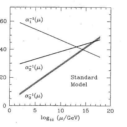
Figure 2: This figure shows the lack of unification of gauge couplings with standard model spectrum. $\alpha^{-1}_{i}$ is plotted against the mass scale and the values at the weak scale are the measures values from LEP and SLC as well as other experiments.

A revival of interest in the idea of grand unification occurred after the ideas of supersymmetry became part of phenomenology of particle physics in the early 80’s. Two points were realized that led to this. First is that a theoretical understanding of the large hierarchy between the weak scale and the GUT scale was possible only within the framework of supersymmetry as discussed in the first chapter. Secondly, on a more phenomenological level, measured values of $sin^{2}\theta_{W}$ from the accelerators coupled with the observed values for $\alpha_{strong}$ and $\alpha_{em}$ could be reconciled with the unification of gauge couplings only if the superpartners were included in the evolution of the gauge couplings and the supersymmetry breaking scale was assumed to be near the weak scale, which was independently motivated anyway[42].

It should be however made clear that supersymmetry is not the only well motivated beyond standard model physics that leads to coupling constant unification consistent with the measured value of $sin^{2}\theta_{W}$. If the neutrinos have masses in the micro-milli-eV range, then the see-saw mechanism[28] given by the formula

$$m_{\nu_{i}}\simeq\frac{m^{2}_{u_{i}}}{M_{B-L}}$$ (36)

implies that the $M_{B-L}$ scale is around $10^{11}$ GeV or so. It was shown in the early 80’s[59] that coupling constant unification can take place without any need for supersymmetry if it is assumed that above the $M_{B-L}$ the gauge symmetry becomes $SU(2)_{L}\times SU(2)_{R}\times U(1)_{B-L}\times SU(3)_{c}$ or $SU(2)_{L}\times SU(2)_{R}\times SU(4)_{c}$. Since the subject of these lectures is supersymmetric grand unification, I will not discuss these models here. Let us now proceed to discuss the unification of gauge couplings in supersymmetric models.

2.1 Unification of Gauge Couplings (UGC)

Key ingredients in this discussion are the renormalization group equations (RGE) for the gauge coupling parameters. Suppose we want to evolve a coupling parameter between the scales $M_{1}$ and $M_{2}$ (i.e. $M_{1}\leq\mu\leq M_{2}$) corresponding to the two scales of physics. Then the RGE’s depend on the gauge symmetry and the field content at $\mu=M_{1}$. The one loop evolution equations for the gauge couplings (define $\alpha_{i}\equiv\frac{g^{2}_{i}}{4\pi}$) are:

$$\frac{d\alpha_{i}}{dt}=\frac{1}{2\pi}b_{i}\alpha^{2}_{i}$$ (37)

where $t=ln\mu$. The coefficient $b_{i}$ receives contributions from the gauge part and the matter including Higgs field part. In general,

$$b_{i}=-3C_{2}(G)+T(R_{1})d(R_{2})$$ (38)

where $C_{2}(R)=\Sigma_{a}R_{a}R_{a}$ and $T(R)\delta^{ab}=Tr(R_{a}R_{b})$. $R_{a}$ are the generators of the gauge group under consideration. The following group theoretical relations are helpful in making actual calculations:

$$C_{2}(R)d(R)=T(R)r$$ (39)

where $d(R)$ is the dimension of the irreducible representation and $r$ is the rank of the group (the number of diagonal generators).

An important point to note is that since at the GUT scale one imagines that the symmetry group merges into one GUT group, all the low energy generators must be normalized the same way. What this means is that if $\Theta_{a}$ are the generators of the groups at low energy, one must satisfy the condition that $Tr(\Theta_{a}\Theta_{b})=2\delta_{ab}$. If we sum over the fermions of the same generation, we easily see that this condition is satisfied for the $SU(2)_{L}$ and the $SU(3)_{c}$ groups. On the other hand, for the hypercharge generator, one must write $\Theta_{Y}=\sqrt{\frac{3}{5}}\frac{Y}{2}$ to satisfy the correct normalization condition. This must therefore be used in evaluating the $b_{1}$.

One can calculate the $b_{i}$ for the MSSM and they are $b_{3}=-3$, $b_{2}=+1$ and $b_{1}=+33/5$ where the subscript $i$ denotes the $SU(i)$ group (for $i>1$) and we have assumed three generations of fermions. The gauge coupling evolution equations can then be written as:

$$2\pi\frac{d\alpha^{-1}_{1}}{dt}=-\frac{33}{5}$$ (40)

$$2\pi\frac{d\alpha^{-1}_{2}}{dt}=-1$$

$$2\pi\frac{d\alpha^{-1}_{3}}{dt}=3$$

The solutions to these equations are:

$$\alpha^{-1}_{1}(M_{Z})=\alpha^{-1}_{U}+\frac{33}{10\pi}ln\frac{M_{U}}{M_{Z}}$$ (41)

$$\alpha^{-1}_{2}(M_{Z})=\alpha^{-1}_{U}+\frac{1}{2\pi}ln\frac{M_{U}}{M_{Z}}$$

$$\alpha^{-1}_{1}(M_{Z})=\alpha^{-1}_{U}-\frac{3}{2\pi}ln\frac{M_{U}}{M_{Z}}$$

If these three equations which have only two free parameters hold then coupling constant unification occurs. These equations lead to the consistency equation[44]:

$$\Delta\alpha\equiv 5\alpha^{-1}_{1}(M_{Z})-12\alpha^{-1}_{2}(M_{Z})+7\alpha^{-1}_{3}(M_{Z})=0$$ (43)

Using the values of the three gauge coupling parameters measured at the $M_{Z}$ scale, i.e.

$$\alpha^{-1}_{1}(M_{Z})=58.97\pm.05$$ (44)

$$\alpha^{-1}_{2}(M_{Z})=29.61\pm.05$$

$$\alpha^{-1}_{3}(M_{Z})=8.47\pm.22$$

(where we have taken for the strong coupling constant the global average given in Ref.[45]), we find that $\Delta\alpha=-1\pm 2$. Thus we see that grand unification of couplings occurs in the one loop approximation. Again subtracting any two of the above evolution equations, we find the unification scale to be $M_{U}\sim 10^{16}$ GeV and $\alpha^{-1}_{U}\simeq 24$.

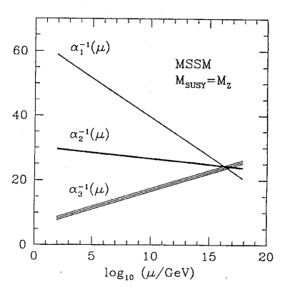
Figure 3: This figure shows the unification of gauge couplings with supersymmetric model spectrum. $\alpha^{-1}_{i}$ is plotted against the mass scale and the values at the weak scale are the measures values from LEP and SLC as well as other experiments.

There are of course two loop effects, corrections arising from the fact that all particle masses may not be degenerate and turn on as a Theta function in the evolution equations etc.[46]. Another point worth noting is that while the value of $\alpha_{1,2}(M_{Z})$ are quite accurately known, the same is not the case for the strong coupling constant and in fact detailed two loop calculations and the MSSM threshold corrections reveal that[47] if the effective MSSM scale ($T_{SUSY}$) is less than $M_{Z}$, one needs $\alpha_{s}(M_{Z})>.121$ to achieve unification. Thus indications of a smaller value for the QCD coupling would indicate more subtle aspects to coupling constant unification such as perhaps intermediate scales[44] or new particles etc.

To better appreciate the degree of unification in supersymmetric models, let us compare this with the evolution of couplings in the standard model. The values of $b_{i}$ for this case are $b_{1}=\frac{41}{10}$, $b_{2}=-\frac{19}{6}$ and $b_{3}=-7$. The gauge coupling unification in this case would require that

$$\Delta\alpha_{sm}=\frac{218}{115}\alpha^{-1}_{3}(M_{Z})-\frac{333}{115}\alpha^{-1}_{2}(M_{Z})+\alpha^{-1}_{1}(M_{Z})=0$$ (45)

Using experimental inputs as before, it easy to check that $\Delta\alpha_{sm}=-11.7$ and is away from zero by many sigma’s.

2.2 Unification Barometer

We see from the above discussion that unification requirement is extremely restrictive and picks out only certain theories which have a specific particle content. It is therefore useful to define a variable that can enable us to test whether a particular theory will unify without performing detailed mass extrapolation but instead by looking at the beta function coefficients. We will call this the “unification barometer”. For this purpose, let define three 3-comp[onent vectors: ${\bf a}=(\alpha^{-1}_{1}(M_{Z}),\alpha^{-1}_{2}(M_{Z}),\alpha^{-1}_{3}(M_{Z}))$, ${\bf u}=\alpha^{-1}_{U}(1,1,1)$ and ${\bf b}=(b_{1},b_{2},b_{3})$ and construct the unification barometer $\Delta\alpha$ as

$$\Delta\alpha={\bf a.u\times b}$$ (46)

For single step unification models, since there are only three variables and three equations, the unification condition amounts to the condition

$$\Delta\alpha=0$$ (47)

Clearly, we have for the standard model, $\Delta\alpha=-11.7$ whereas for the MSSM particle content, $\Delta\alpha=-.5\pm 3.5$ which is another way to view the above conclusions regarding unifiability of the MSSM.

We will see that for models with intermediate scales, this variable provides a simpler way to tell whether a given theory will unify or not.

2.3 Gauge coupling unification with intermediate scales before grand unification

An important aspect of grand unification is the possibility that there are intermediate symmetries before the grand unification symmetry is realized. For instance a very well motivated example is the presence of the gauge group $SU(2)_{L}\times SU(2)_{R}\times U(1)_{B-L}\times SU(3)_{c}$ before the gauge symmetry enlarges to the SO(10) group. So it is important to discuss how the evolution equation equations are modified in such a situation.

Suppose that at the scale $M_{I}$, the gauge symmetry enlarges. To take this into account, we need to follow the following steps:

(i) If the smaller group $G_{1}$ gets embedded into a single bigger group $G_{2}$ at $M_{I}$, then at the one loop level, we simply impose the matching condition:

$$g_{1}(M_{I})=g_{2}(M_{I})$$ (48)

(ii) On the other hand if the generators of the low scale symmetry arise as linear combinations of the generators of different high scale groups as follows:

$$\lambda_{1}=\Sigma_{b}p_{b}\theta_{b}$$ (49)

then the coupling matching condition is:

$$\frac{1}{g^{2}_{1}(M_{I})}=\Sigma_{b}\frac{p^{2}_{b}}{g^{2}_{b}(M_{I})}$$ (50)

One can prove this as follows: for simplicity let us consider only the case where $G_{2}=\Pi_{b}U(1)_{b}$ which at $M_{I}$ breaks down to a single $U(1)$. Let this breaking occur via the vev of a single Higgs field $\phi$ with charges $(q_{1},q_{2},....)$ under $U(1)$. The unbroken generator is given by:

$$Q=\Sigma p_{a}Q_{a}$$ (51)

with $\Sigma_{c}p_{c}q_{c}=0$. The gauge field mass matrix after Higgs mechanism can be written as

$$M^{2}_{ab}=g_{a}g_{b}q_{a}q_{b}<\phi>^{2}$$ (52)

This mass matrix has the following massless eigenstate which can be identified with the unbroken U(1) gauge field:

$$A_{\mu}=\frac{1}{(\Sigma_{b}\frac{p^{2}_{b}}{g^{2}_{b}})^{1/2}}\Sigma\frac{p_{b}}{g_{b}}A_{\mu,b}\equiv N\Sigma_{b}\frac{p^{2}_{b}}{g^{2}_{b}}A_{\mu,b}$$ (53)

To find the effective gauge coupling, we write

$$L\sim\Sigma g_{b}Q_{b}A_{\mu,b}$$ (54)

$$=\Sigma_{b}g_{b}(p_{b}Q+...)N(\frac{p_{b}}{g_{b}}A_{\mu}+...)$$

Collecting the coefficient of $A_{\mu}$ and using the normalization condition $\Sigma p^{2}_{b}=1$, we get the result we wanted to prove (i.e. Eq.).

Let us apply this to the situation where $SU(2)_{R}\times U(1)_{B-L}$ is broken down to $U(1)_{Y}$. In that case:

$$\frac{Y}{2}=I_{3,R}+\frac{B-L}{2}$$ (55)

The normalized generators are $I_{Y}=\left(\frac{3}{5}\right)^{1/2}\frac{Y}{2}$ and $I_{B-L}=\left(\frac{3}{2}\right)^{1/2}\frac{B-L}{2}$. Using them, one finds that

$$I_{Y}=\sqrt{\frac{3}{5}}I_{3R}+\sqrt{\frac{2}{5}}I_{B-L}$$ (56)

This implies that the matching of coupling constant at the scale where the left-right symmetry begins to manifest itself is given by:

$$\alpha^{-1}_{Y}=\frac{3}{5}\alpha^{-1}_{2R}+\frac{2}{5}\alpha^{-1}_{B-L}$$ (57)

Application to SO(10) GUT and possibility of low $W_{R}$ scale

Let us apply this to the SO(10) model to see under what conditions a low $W_{R}$ mass can be consistent with coupling constant unification. Let us first derive the evolution equations for the couplings in $SO(10)$ model with an intermediate $W_{R}$ scale. For the $\alpha_{2}$ and $\alpha_{3}$, the evolution equations are straightforward and given by:

$$\alpha^{-1}_{i}(M_{Z})=\alpha^{-1}_{U}-\frac{b_{i}}{2\pi}ln\frac{M_{R}}{M_{Z}}-\frac{b^{\prime}_{i}}{2\pi}ln\frac{M_{U}}{M_{R}}$$ (58)

where $i=2,3$ and $b^{\prime}_{i}$ receives contributions from all particles at and below the scale $M_{R}$. We assume that there are no other particles between $M_{R}$ and $M_{U}$ other than those included in $b_{i}$. Turning to $\alpha_{1}$, we have to use the matching formula for the couplings derived above. Using that, we find that

$$\alpha^{-1}_{1}(M_{Z})=\alpha^{-1}_{1}(M_{R})-\frac{b_{1}}{2\pi}ln\frac{M_{R}}{M_{Z}}$$ (59)

Using the matching formula derived above, and evolving the $\alpha_{2R,B-L}$ between $M_{R}$ and $M_{U}$, we find that

$$\alpha^{-1}_{1}(M_{Z})=\alpha^{-1}_{U}-\frac{b_{1}}{2\pi}ln\frac{M_{R}}{M_{Z}}-(\frac{3}{5}\frac{b^{\prime}_{2R}}{2\pi}-\frac{2}{5}\frac{b^{\prime}_{BL}}{2\pi})ln\frac{M_{U}}{M_{R}}$$ (60)

In the discussion that follows let us denote $3/5b^{\prime}_{2R}+2/5b^{\prime}_{BL}\equiv b^{\prime}_{1}$. We then see that a sufficient condition for the intermediate scale to exist is that we must have

$$\Delta\alpha_{SUSY}\equiv 5b^{\prime}_{1}-12b^{\prime}_{2L}+7b^{\prime}_{3}=0$$ (61)

In fact if this condition is satisfied, at the one loop level, one can even have a $W_{R}$ mass in the TeV range and still have coupling constant unification. As an example of such a theory, consider the following spectrum of particles above $M_{R}$: a color octet, a pair of $SU(2)_{R}$ triplets with $B-L=\pm 2$, two bidoublets $\phi(2,2,0)$ and a left-handed triplet. The corresponding b-coefficients above $M_{R}$ are given by:

$$b^{\prime}_{3}=0;b^{\prime}_{2L}=4;b^{\prime}_{2R}=6~{}~{}and~{}~{}b^{\prime}_{BL}=15$$ (62)

This theory satisfies the condition that $\Delta\alpha_{SUSY}=0$ and can support a low $W_{R}$ theory.

In general, the unifiability condition translates to

$$\Delta\alpha=y\Delta\alpha^{\prime}$$ (63)

where $y=\frac{1}{2\pi}ln\frac{M_{U}}{M_{I}}$ and $\Delta\alpha^{\prime}={\bf a.u\times b^{\prime}}$.

2.4 Yukawa unification

Another extension of the idea of gauge coupling unification is to demand the unification of Yukawa coupling parameters and study its implications and predictions. This however is a much more model dependent conjecture than the UGC[48]. One may of course demand partial Yukawa unification instead of a complete one between all three generations. As we will see in the next chapter, most grand unification models tend to imply partial Yukawa unification of type:

$$h_{b}(M_{U})=h_{\tau}(M_{U})$$ (64)

To discuss the implications of this hypothesis, we need the renormalization group evolution of these couplings down to the weak scale. For this purpose, we need the R.G.E’s for these couplings:

$$2\pi\frac{dlnY_{b}}{dt}=6Y_{b}+Y_{t}-\frac{7}{15}\alpha_{1}-\frac{16}{3}\alpha_{3}-3\alpha_{2}$$ (65)

$$2\pi\frac{dlnY_{\tau}}{dt}=4Y_{\tau}-\frac{9}{5}\alpha_{1}-3\alpha_{2}$$

$$2\pi\frac{dlnY_{t}}{dt}=6Y_{t}+Y_{b}-\frac{13}{15}\alpha_{1}-\frac{16}{3}\alpha_{3}-3\alpha_{2}$$

where we have defined $Y_{i}\equiv h^{2}_{i}/4\pi$. Subtracting the first two equations in Eq. (59) and defining $R_{b/\tau}\equiv\frac{Y_{b}}{Y_{\tau}}$, one finds that

$$2\pi\frac{d}{dt}(R_{b/\tau})\simeq(Y_{t}-\frac{16}{3}\alpha_{3})$$ (66)

Solving this equation using the Yukawa unification condition, we find that

$$\frac{m_{b}}{m_{\tau}}(M_{Z})=(R_{b/\tau}(M_{Z}))^{1/2}=A^{-1/2}_{t}\left(\frac{\alpha_{3}(M_{Z})}{\alpha_{3}(M_{U})}\right)^{8/9}$$ (67)

where $A_{t}=e^{\frac{1}{2\pi}\int^{M_{U}}_{M_{Z}}Y_{t}dt}$. Using the value of $\alpha_{U}$ from MSSM grand unification, we find that $m_{b}/m_{\tau}(M_{Z})\simeq 2.5A^{-1/2}_{t}$. The observed value of $m_{b}/m_{\tau}(M_{Z})\simeq 1.62$. So it is clear that a significant contribution from the running of the top Yukawa is needed and this is lucky since the top quark is now known to have mass of $\sim 175$ GeV implying an $h_{t}\simeq 1$. One way to estimate the $A_{t}$ is to assume that $h_{t}(M_{U})=3$, which case one has[49] $A^{-1/2}\simeq.85$ making $m_{b}/m_{\tau}$ closer to observations.

It is worth pointing out that both the top Yukawa as well as the gauge contributions depend on whether there exist an intermediate scale. The modified formula in that case is

$$\frac{m_{b}}{m_{\tau}}(M_{Z})=(A^{ZI}_{t}A^{IU}_{t})^{-1/2}\left(\frac{\alpha_{3}(M_{Z})}{\alpha_{3}(M_{I})}\right)^{8/9}\left(\frac{\alpha_{3}(M_{I})}{\alpha_{3}(M_{U})}\right)^{8/3b^{\prime}_{3}}$$ (68)

(A) Top Yukawa coupling and its infrared fixed point

It was noted by Hill and Pendleton and Ross[50] for large Yukawa couplings, $h_{t}$, regardless of how large the asymptotic value is, the low energy value determined by the RGE’s is a fixed value and one can therefore use this observation to predict the top quark mass. To see this in detail, let us define a parameter $\rho_{t}=Y_{t}/\alpha_{3}$. Using the RGE’s for $Y_{t}$ and $\alpha_{3}$, we can then write

$$\alpha_{3}\frac{d\rho_{t}}{d\alpha_{3}}=-2\rho_{t}(\rho_{t}-\frac{7}{18})$$ (69)

The solution of this equation is

$$\rho_{t}(\alpha_{3})=\frac{7/8}{1-(1-\frac{7}{18\rho_{t0}})(\frac{\alpha_{3}}{\alpha_{30}})^{-7/9}}$$ (70)

where $\rho_{t0}=\rho_{t}(\Lambda)$ and $\alpha_{30}=\alpha_{3}(\Lambda)$. As we move to smaller $\mu$’s, $\alpha_{3}$ increases and as $\alpha_{3}\rightarrow$infinity, $\rho_{t}\rightarrow 7/18$. This leads to $m_{t}=129sin\beta$ GeV which is much smaller than the observed value. Does this mean that this idea does not work ? The answer is no because, strictly, at $m_{t}(m_{t})$, the $\alpha_{3}$ is far from being infinity. A more sensible thing to do is to use the RGE’s for $Y_{t}$ and assume that at $\Lambda\gg M_{Z}$, $Y_{t}\gg\alpha_{3}$ so that for very large $\mu$, we have

$$\frac{dY_{t}}{dt}\simeq\frac{3Y^{2}_{t}}{\pi}$$ (71)

As a result, as we move down from $\Lambda$, first $Y_{t}$ will decrease till it bocomes comparable to $\alpha_{3}$ after which, it will settle down to the value $6Y_{t}=16/3\alpha_{3}$ for which $Y_{t}$ stops running. This leads to a prediction of $m_{t}\simeq 196sin\beta$ GeV, which is more consistent with observations. Note incidentally that if we applied the same arguments to the standard model, we would obtain $m_{t}\simeq 278$ GeV, which is much too large. Could this be an indication that supersymmetry is the right way to go in understanding the top quark mass ?

Finally, we wish to very briefly mention that one could have demanded complete Yukawa unification as is predicted by simple SO(10) models[48]:

$$h_{t}(M_{U})=h_{b}(M_{U})=h_{\tau}(M_{U})\equiv h_{U}$$ (72)

Extrapolating this relation to $M_{Z}$ one could obtain $m_{t},m_{b},m_{\tau}$ in terms of only two parameters $h_{U}$ and $tan\beta$. This would be a way to also predict $m_{t}$. This is therefore an attractive idea. But getting the electroweak symmetry breaking in this scenario is very hard since both $m^{2}_{H_{u}}$ and $m^{2}_{H_{d}}$ run parallel to each other except for a minor difference arising from the $U(1)_{Y}$ effects. One therefore has to make additional assumptions to understand the electroweak symmetry breaking out of radiative corrections. One of the ways is to use the D-terms, as has been shown in Ref.[51].

2.5 Updating the discussion of mass scales in the light of grand unification

Since the idea of grand unification has introduced another new mass scale into theories (i.e. $M_{U}\simeq 2\times 10^{16}$ GeV), let us recapitulate the new situation. As we saw before, with the advent of supersymmetry, one could (in some versions) replace the $M_{W_{L}},M_{P\ell}$ with the $\Lambda_{SUSY}\simeq 10^{11}~{}GeV,M_{P\ell}\simeq 2\times 10^{18}~{}GeV$. With grand unification we have a new scale in between. Thus we have these three scales to explain in any final theory.

3 Supersymmetric SU(5)

The simplest supersymmetric grand unification model is based on the simple group SU(5)[68] and it embodies many of the unification ideas discussed in the previous chapter. It is assumed that at the GUT scale $M_{U}$, SU(5) gauge symmetry breaks down to MSSM as follows:

$$SU(5)\rightarrow SU(3)_{c}\times SU(2)_{L}\times U(1)_{Y}$$ (73)

The unification ideas of the previous section tell us that the single gauge coupling at the GUT scale branches down to the three couplings of the standard model.

3.1 Particle assignment and symmetry breaking

To discuss further properties of the model, we discuss the assignment of the matter fields as well as the Higgs superfields to the simplest representations necessary. The matter fields are assigned to the $\bar{5}\equiv\bar{F}$ and $10\equiv 10$ dimensional representations whereas the Higgs fields are assigned to $\Phi\equiv 45$, $H\equiv{5}$ and $\bar{H}\equiv\bar{5}$ representations.

Matter Superfields:

$$\bar{F}=\left(\begin{array}[]{c}d^{c}_{1}\\ d^{c}_{2}\\ d^{c}_{3}\\ e^{-}\\ \nu\end{array}\right)\\ ;T\{10\}=\left(\begin{array}[]{ccccc}0&u^{c}_{3}&-u^{c}_{2}&u_{1}&d_{1}\\ -u^{c}_{3}&0&u^{c}_{1}&u_{2}&d_{2}\\ u^{c}_{2}&-u^{c}_{1}&0&u_{3}&d_{3}\\ -u_{1}&-u_{2}&u_{3}&0&e^{+}\\ -d_{1}&-d_{2}&-d_{3}&-e^{+}&0\end{array}\right)$$

In the following discussion, we will choose the group indices as $\alpha,\beta$ for SU(5); (e.g.$H^{\alpha},\bar{H}_{\alpha},\bar{F}_{\alpha},T^{\alpha\beta}=-T^{\beta\alpha}$ ); $i,j,k..$ will be used for $SU(3)_{c}$ indices and $p,q$ for $SU(2)_{L}$ indices.

To discuss symmetry breaking and other dynamical aspects of the model, we choose the superpotential to be:

$$W=W_{Y}+W_{G}+W_{h}+W\prime$$ (74)

where

$$W_{Y}=h_{u}^{ab}\epsilon_{\alpha\beta\gamma\delta\sigma}T_{a}^{\alpha}\beta T_{b}^{\gamma\delta}H^{\sigma}+h_{d}^{a}bT^{\alpha\beta}\bar{F}_{\alpha}\bar{H}_{\beta}$$ (75)

($a,b$ are generation indices). This part of the superpotential is resposible for giving mass to the fermions.

$$W_{G}=zTr\Phi+xTr{\Phi}^{2}+yTr{\Phi}^{3}+\lambda_{1}(H\Phi\bar{H}+MH\bar{H})$$ (76)

This part of the superpotential is responsible for symmetry breaking and getting light Higgs doublets below $M_{U}$. Note that although $Tr\Phi=0$ the z-term added as a Lagrange multiplier to enforce this constraint during potential minimization. Of the rest of the superpotential $W_{h}$ is the Hidden sector superpotential responsible for supersymmetry breaking and $W^{\prime}$ denotes the R-parity breaking terms which will be discussed later. We are looking for the following symmetry breaking chain:

$$SU(5)\times SUSY\rightarrow<\Phi>\neq 0\rightarrow G_{std}\times SUSY$$ (77)

To study this we have to use $W_{G}$ and calculate the relevant F-terms and set them to zero to maintain supersymmetry down to the weak scale.

$$F^{\alpha}_{\Phi,\beta}=z\delta^{\alpha}_{\beta}+2x\Phi^{\alpha}_{\beta}+3y\Phi^{\alpha}_{\gamma}\Phi^{\gamma}_{\beta}=0$$ (78)

Taking $<Tr\Phi>=0$ implies that $z=-\frac{3}{5}y<Tr\Phi^{2}>$. If we assume that $Diag<\Phi>=(a_{1},a_{2},a_{3},a_{4},a_{5})$, then one has the following equations:

$$\Sigma_{i}a_{i}=0$$ (79)

$$z+2xa_{i}+3ya^{2}_{i}=0$$

with $i=1,...5$. Thus we have five equations and two parameters. There are therefore three different choices for the $a_{i}$’s that can solve the above equations and they are: Case (A):

$$<\Phi>=0$$ (80)

In this case, SU(5) symmetry remains unbroken. Case (B):

$$Diag<\Phi>=(a,a,a,a,-4a)$$ (81)

In this case, SU(5) symmetry breaks down to $SU(4)\times U(1)$ and one can find $a=\frac{2x}{9y}$. Case (C):

$$Diag<\Phi>=(b,b,b,-\frac{3}{2}b,-\frac{3}{2}b)$$ (82)

This is the desired vacuum since SU(5) in this case breaks down to $SU(3)_{c}\times SU(2)_{L}\times U(1)_{Y}$ gauge group of the standard model. The value of $b=\frac{4x}{3y}$ and we choose the parameters $x$ to be order of $M_{U}$. In the supersymmetric limit all vacua are degenerate.

3.2 Low energy spectrum and doublet-triplet splitting

Let us next discuss whether the MSSM arises below the GUT scale in this model. So far we have only obtained the gauge group. The matter content of the MSSM is also already built into the $\bar{F}$ and $T$ multiplets. The only remaining question is that of the two Higgs superfields $H_{u}$ and $H_{d}$ of MSSM. They must come out of the $H$ and the $\bar{H}$ multiplets. Writing $H\equiv\left(\begin{array}[]{c}\zeta_{u}\\ H_{u}\end{array}\right)$ and $\bar{H}\equiv\left(\begin{array}[]{c}\bar{\zeta_{d}}\\ H_{d}\end{array}\right)$. From $W_{G}$ substituting the $<\Phi>$ for case (C), we obtain,

$$W_{eff}=\lambda(b+M)\zeta_{u}\bar{\zeta_{d}}+\lambda(-3/2b+M)H_{u}H_{d}$$ (83)

If we choose $3/2b=M$, then the massless standard model doublets remain and every other particle of the SU(5) model gets large mass. The uncomfortable aspect of this procedure is that the adjustment of the parameters is done by hand does not emerge in a natural manner. This procedure of splitting of the color triplets $\zeta_{u,d}$ from $SU(2)_{L}$ doublets $H_{u,d}$ is called doublet-triplet splitting and is a generic issue in all GUT models. An advantage of SUSY GUT’s is that once the fine tuning is done at the tree level, the nonrenormalization theorem of the SUSY models preserves this to all orders in perturbation theory. This is one step ahead of the corresponding situation in non- SUSY GUT’s, where the cancellation between $b$ and $M$ has to be done in each order of perturbation theory. A more satisfactory situation would be where the doublet-triplet splitting emerges naturally due to requirements of group theory or underlying dynamics.

3.3 Fermion masses and Proton decay

Effective superpotential for matter sector at low energies then looks like:

$$W_{matter}~{}=~{}h_{u}QH_{u}u^{c}+h_{d}QH_{d}d^{c}+h_{l}LH_{d}e^{c}+\mu H_{u}H_{d}$$ (84)

Note that $h_{d}$ and $h_{l}$ arise from the $T\bar{F}\bar{H}$ coupling and this satisfies the relation $h_{d}=h_{l}$. Similarly, $h_{u}$ arises from the $TTH$ coupling and therefore obeys the constraint $h_{u}=h^{T}_{u}$. (None of these constraints are present in the MSSM). The second relation will be recognized by the reader as a partial Yukawa unification relation and we can therefore use the discussion of Section 2 to predict $m_{\tau}$ in terms of $m_{b}$. The relation between the Yuakawa couplings however holds for each generation and therefore imply the undesirable relations among the fermion masses such as $m_{d}/m_{s}=m_{e}/m_{\mu}$. This relation is independent of the mass scale and therefore holds also at the weak scale. It is in disagreement with observations by almost a factor of 15 or so. This a major difficulty for minimal SU(5) model. This problem does not reflect any fundamental difficulty with the idea of grand unification but rather with this particular realization. In fact by including additional multiplets such as ${\bf 45}$ in the theory, one can avoid this problem. Another way is to add higher dimensional operators to the theory such as $T\bar{F}\Phi\bar{H}/M_{Pl}$, which can be of order 0.1 GeV or so and could be used to fix the muon mass prediction from $SU(5)$.

The presence of both quarks and leptons in the same multiplet of SU(5) model leads to proton decay. For detailed discussions of this classic feature of GUTs, see for instance [2]. In non-SUSY SU(5), there are two classes of Feynman diagrams that lead to proton decay in this model: (i) the exchange of gauge bosons familiar from non-SUSY SU(5) where effective operators of type $e^{+\dagger}ud^{c\dagger}u$ are generated; and (ii) exchange of Higgs fields. In the supersymmetric case there is an additional source for proton decay coming from the exchange of Higgsinos, where $QQH$ and $QL\bar{H}$ via $H\bar{H}$ mixing generate the effective operator $QQQL/M_{H}$ that leads to proton decay. In fact, this turns out to give the dominant contribution.

The gauge boson exchange diagram leads to $p\rightarrow e^{+}\pi^{0}$ with an amplitude $M_{p\rightarrow e^{+}\pi^{0}}\simeq\frac{4\pi\alpha_{U}}{M^{2}_{U}}$. This leads to a prediction for the proton lifetime of:

$$\tau_{p}=4.5\times 10^{29\pm.7}\left(\frac{M_{U}}{2.1\times 10^{14}~{}GeV}\right)^{4}$$ (85)

For $M_{U}\simeq 2\times 10^{16}$ GeV, one gets $\tau_{p}=4.5\times 10^{37\pm.7}$ yrs. This far beyond the capability of SuperKamiokande experiment, whose ultimate limit is $\sim 10^{34}$ years.

Turning now to the Higgsino exchange diagram, we see that the amplitude for this case is given by:

$$M\simeq\frac{h_{u}h_{d}}{M_{H}}\cdot\frac{m_{gaugino}g^{2}}{16\pi^{2}M^{2}_{\tilde{Q}}}$$ (86)

In this formula there is only one heavy mass suppression. Although there are other suppression factors, they are not as potent as in the gauge boson exchange case. As a result, this dominates. A second aspect of this process is that the final state is $\nu K^{+}$ rather than $e^{+}\pi^{0}$. This can be seen by studying the effective operator that arises from the exchange of the color triplet fields in the ${\bf 5}+{\bf\bar{5}}$ i.e. $O_{\Delta B=1}=QQQL$ where $Q$ and $L$ are all superfields and are therefore bosonic operators. In terms of the isospin and color components, this looks like $\epsilon^{ijk}u_{i}u_{j}d_{k}e^{-}$ or $\epsilon^{ijk}u_{i}d_{j}d_{k}\nu$. It is then clear that unless the two $u$’s or the $d$’s in the above expressions belong to two different generations, the operators vanishes due to color antisymmetry. Since the charm particles are heavier than the protons, the only contribution comes from the second operators and the strange quark has to be present (i.e. the operator is $\epsilon^{ijk}u_{i}d_{j}s_{k}\nu_{\mu}$. Hence the new final state. Detailed calculations show[53] that for this decay lifetime to be consistent with present observations, one must have $M_{H}>M_{U}$ by almost a factor of 10. This is somewhat unpleasant since it would require that some coupling in the superpotential has to be much larger than one.

3.4 Other aspects of SU(5)

There are several other interesting implications of SU(5) grand unification that makes this model attractive and testable. The model has very few parameters and hence is very predictive. The MSSM has got more than a hundred free parameters, that makes such models expertimentally quite fearsome and of course hard to test. On the other hand, once the model is embedded into SUSY SU(5) with Polonyi type supergravity, the number of parameters reduces to just five: they are the $A,~{}B,~{}m_{3/2}$ which parameterize the effects of supergravity discussed in section I, $~{}\mu$ parameter which is the $H_{u}H_{d}$ mixing term in the superpotential also present in the superpotential and $m_{\lambda}$, the universal gaugino mass. This reduction in the number of parameters has the following implications:

(i) Gaugino unification:

At the GUT scale, we have the three gaugino masses equal (i.e. $m_{\lambda_{1}}=m_{\lambda_{2}}=m_{\lambda_{3}}$. Their values at the weak scale can be predicted by using the RG running as follows:

$$\frac{dm_{\lambda_{i}}}{dt}=\frac{b_{i}}{2\pi}\alpha_{i}m_{\lambda_{i}}$$ (87)

Solving these equations , one finds that at the weak scale, we have

$$m_{\lambda_{1}}:m_{\lambda_{2}}:m_{\lambda_{3}}=\alpha_{1}:\alpha_{2}:\alpha_{3}$$ (88)

Thus discovery of gauginos will test this formula and therefore SU(5) grand unification.

(ii) Prediction for squark and slepton masses

At the supersymmetry breaking scale, all scalar masses in the simple supergravity schemes are equal. Again, one can predict their weak scale values by the RGE extrapolation. One finds the following formulae[54]:

$$m^{2}_{\tilde{Q}}=m^{2}_{3/2}+m^{2}_{Q}+\frac{\alpha_{U}}{4\pi}[\frac{8}{3}f_{3}+\frac{3}{2}f_{2}+\frac{1}{30}f_{1}]m^{2}_{\lambda_{U}}+Q^{Z}_{Q}M^{2}_{Z}cos^{2}2\beta$$ (89)

where $Q^{Z}_{u}=\frac{1}{2}-\frac{2}{3}sin^{2}\theta_{W}$ and $Q^{Z}_{d}=-\frac{1}{2}+\frac{1}{3}sin^{2}\theta_{W}$ and $f_{k}=\frac{t(2-b_{k}t)}{1+b_{k}t^{2}}$ and $b_{k}$ are the coefficients of the RGE’s for coupling constant evolutions given earlier. A very obvious formula for the sleptons can be written down. It omits the strong coupling factor. A rough estimate gives that $m^{2}_{\tilde{l}}\simeq m^{2}_{3/2}$ and $m^{2}_{\tilde{Q}}\simeq m^{2}_{3/2}+4m^{2}_{\lambda_{U}}$. This could therefore serve as independent tests of the SUSY SU(5).

3.5 Problems and prospects for SUSY SU(5)

While the simple SUSY SU(5) model exemplifies the power and utility of the idea of SUSY GUTs, it also brings to the surface some of the problems one must solve if the idea eventually has to be useful. Let us enumerate them one by one and also discuss the various ideas proposed to overcome them.

(i) R-parity breaking:

There are renormalizable terms in the superpotential that break baryon and lepton number:

$$W^{\prime}=\lambda_{abc}T_{a}\bar{F}_{b}\bar{F}_{c}$$ (90)

When written in terms of the component fields, this leads to R-parity breaking terms of the MSSM such as $L_{a}L_{b}e^{c}_{c}$, $QLd^{c}$ as well as $u^{c}d^{c}d^{c}$ etc. The new point that results from grand unification is that there is only one coupling parameter that describes all three types of terms and also the coupling $\lambda$ satisfies the antisymmetry in the two generation indices $b,c$. This total number of parameters that break R-parity are nine instead of 45 in the MSSM. There are also nonrenormalizable terms of the form $T\bar{F}\bar{F}(\Phi/M_{P\ell})^{n}$[55], which are significant for $n=1,2,3,4$ and can add different complexion to the R-parity violation. Thus, the SUSY SU(5) model does not lead to an LSP that is naturally stable to lead to a CDM candidate. As we will see in the next section, the SO(10) model provides a natural solution to this problem if only certain Higgs superfields are chosen.

(ii) Doublet-triplet splitting problem:

We saw earlier that to generate the light doublets of the MSSM, one needs a fine tuning between the two parameters $3/2\lambda b$ and $M$ in the superpotential. However once SUSY breaking is implemented via the hidden sector mechanism one gets a SUSY breaking Lagrangian of the form:

$$L_{SB}=A\lambda\bar{H}\Phi H+BM\bar{H}H+h.c.$$ (91)

where the symbols in this equation are only the scalar components of the superfields. In general supergravity scenarios, $A\neq B$. As a result, when the Higgsinos are fine tuned to have mass in the weak scale range, the same fine tuning does not leave the scalar doublets at the weak scale.

There are two possible ways out of this problem: we discuss them below.

(iiA) Sliding singlet

The first way out of this is to introduce a singlet field $S$ and choose the superpotential of the form:

$$W_{DT}=2\bar{H}\Phi H+S\bar{H}H$$ (92)

The supersymmetric minimum of this theory is given by:

$$F_{H}=H_{u}(-3b+<S>)=0$$ (93)

The $F_{\zeta}$ equation is automatically satisfied when color is unbroken as is required to make the theory physically acceptable. We then see that one then automatically gets $<S>=3b$ which is precisely the condition that keeps the doublets light. Thus the doublets remain naturally of the weak scale without any need for fine tuning. This is called the sliding singlet mechanism. In this case the supersymmetry breaking at the tree level maintains the masslessness of the MSSM doublets for both the fermion as well as the bosonic components. There is however a problem that arises once one loop corrections are included- because they lead to corrections for the $<S>$ vev of order $\frac{1}{16\pi^{2}}m_{3/2}M_{U}$ which then produces a mismatch in the cancellation of the bosonic Higgs masses. One is back to square one!

(iiB) Missing partner mechanism:

A second mechanism that works better than the previous one is the so called missing partner mechanism where one chooses to break the GUT symmetry by a multiplet that has coupling to the $H$ and $\bar{H}$ and other multiplets in such a way that once SU(5) symmetry is broken, only the color triplets in them have multiplets in the field it couples to pair up with but not weak doublets. As a result, the doublet is naturally light. An example is provided by adding the 50, $\bar{\bf 50}$ (denoted by $\Theta^{\alpha\beta}_{\gamma\delta\sigma}$ and $\bar{\Theta}$ respectively) and replacing 24 by the 75 (denoted $\Sigma$) dimensional multiplet. Note that 75 dim multiplet has a standard model singlet in it so that it breaks the SU(5) down to the standard model gauge group. At the same time 50 has a color triplet only and no doublet. The ${\bf 50.75.\bar{5}}$ coupling enables the color triplet in 50 and $\bar{\bf 5}$ to pair up leaving the weak doublet in $\bar{H}$ light. The superpotential in this case can be given by

$$W_{G}=\lambda_{1}\Theta\Sigma H+\lambda_{2}\bar{\Theta}\Sigma\bar{H}+M\Theta\bar{\Theta}+f(\Sigma)$$ (94)

This mechanism can be applied in the case of other groups too.

(iii) Baryogenesis problem

There are also other problems with the SUSY SU(5) model that suggest that other GUT groups be considered. One of them is the problem with generating the baryon asymmetry of the universe in a simple manner. The point is that if baryon asymmetry in this model is generated at the GUT scale as is customarily done, then there must also simultaneously be a lepton asymmetry such that $B-L$ symmetry is preserved. The reason for this is that all interactions of the simple SUSY models conserve B-L symmetry. As a result, we can write the $n_{B}=\frac{1}{2}n_{B-L}+\frac{1}{2}n_{B+L}=\frac{1}{2}n_{B+L}$. The problem then is that the sphaleron interactions[56] which are in equilibrium for $10^{2}~{}GeV\leq T\leq 10^{12}~{}GeV$, will erase the $n_{B+L}$ since they violate the $B+L$ quantum number. Thus the GUT scale baryon asymmetry cannot survive below the weak scale. Of course one could perhaps generate baryons at the weak scale using the sphaleron processes. But no simple and convincing mechanism seems to have been in place yet. Thus it may be wise to look at higher unification groups.

(iv) Neutrino masses

Finally, in the SU(5) model there seems to be no natural mechanism for generating neutrino masses although using the R-parity violating interactions for such a purpose has often been suggested. One would then have to accept that the required smallness of their couplings has to be put in by hand.

(v) Vacuum degeneracy and supergravity effects

A generic cosmological problem of most SUSY GUT’s is the vacuum degeneracy obtained in the case of the SU(5) model in the supersymmetric limit discussed in section 3.2 above. Recall that SU(5) symmetry breaking via the 24 Higgs superfield leaves three vacua i.e. the SU(5) , $SU(4)\times U(1)$ and the $SU(3)_{c}\times SU(2)_{L}\times U(1)_{Y}$ ones with same vacuum energy. The question then is how does the universe settle down to the standard model vacuum. It turns out that once the supergravity effects are included, the three vacua have different energies coming from the $\frac{-3}{M^{2}_{Pl}}|W|^{2}$ term in the effective bosonic potential. Using the values of the parameters a and b above that characterise the vacua, we find these energies to be:

$$<\Phi>=0:V_{0}=0$$ (95)

$$SU(4)\times U(1):V_{0}=-3\left(\frac{80}{243}\right)^{2}\frac{x^{6}}{M^{2}_{Pl}y^{4}}$$

$$SU(3)_{c}\times SU(2)_{L}\times U(1)_{y}:V_{0}=-3\frac{1600}{81}\frac{x^{6}}{M^{2}_{Pl}y^{4}}$$

This would appear quite interesting since indeed the standard model vacuum has the lowest vacuum energy. However that is misleading since this evaluation is done prior to the setting of the cosmological constant to zero. Once that is done, the standard model indeed acquires the highest vacuum energy. Thus this remains a problem. One way to avoid this would be to imagine that the standard model is indeed stuck in the wrong vacuum but the tunneling probability to other vacua is negligible or at least it is such that the tunnelling time is longer than the age of the universe.

It is worth pointing out that in the case where the SU(5) symmetry is broken by the 75 dim. multiplet, there is no $SU(4)\times U(1)$ inv. vacuum. Similarly one can imagine eliminating the SU(5) inv vacuum by adding to the superpotential terms like $S(\Sigma^{2}-M^{2}_{U})$.

4 Supersymmetric SO(10)

In this section, we like to discuss supersymmetric SO(10) models which have a number of additional desirable features over SU(5) model. For instance, all the matter fermions fit into one spinor representation of SO(10); secondly, the SO(10) spinor being 16-dimensional, it contains the right-handed neutrino leading to nonzero neutrino masses. The gauge group of SO(10) is left-right symmetric which has the consequence that it can solve the SUSY CP problem and R-parity problem etc. of the MSSM unlike the SU(5) model. Before proceeding to a discussion of the model, let us briefly discuss the group theory of SO(10).

4.1 Group theory of SO(10)

The SO(2N) group is defined by the Clifford algebra of 2N elements, $\Gamma_{a}$ which satisfy the following anti-commutation relations:

$$[\Gamma_{a},\Gamma_{b}]_{+}=2\delta_{ab}$$ (96)

where $a,b$ go from 1…2N. The generators of SO(2N) group are then given by $\Sigma_{ab}\equiv\frac{1}{2i}[\Gamma_{a},\Gamma_{b}]_{-}$. The study of the spinor representations and simple group theoretical manipulations with SO(2N) is considerably simplified if one uses the SU(N) basis for SO(2N)[57].

To discuss the SU(N) basis, let us introduce N anticommuting operators $\chi_{i}$ and $\chi^{\dagger}_{i}$ satisfying the following anticommuting relations:

$$[\chi_{i},\chi^{\dagger}_{j}]_{+}=\delta_{ij}$$ (97)

We can then express the elements of the Clifford algebra $\Gamma_{a}$’s in terms of these fermionic operators as follows:

$$\Gamma_{2i-1}=\frac{\chi_{i}-\chi^{\dagger}_{i}}{2i}$$ (98)

$$\Gamma_{2i}=\frac{\chi_{i}+\chi^{\dagger}_{i}}{2}$$

The spinor representations of the SO(10) group can be obtained using this formalism as follows:

$$\Psi=\left(\begin{array}[]{c}\chi^{\dagger}_{j}|0>\\ \chi^{\dagger}_{j}\chi^{\dagger}_{k}\chi^{\dagger}_{l}|0>\\ \chi^{\dagger}_{j}\chi^{\dagger}_{i}\chi^{\dagger}_{l}\chi^{\dagger}_{m}\chi^{\dagger}_{n}|0>\end{array}\right)$$ (102)

By simple counting, one can see that this is a 16 dimensional representation. The states in the 16-dim. spinor have the right quantum numbers to accomodate the matter fermions of one generation. The different particle states can be easily identified: e.g. $e^{-}=\chi^{\dagger}_{4}|0>$; $d^{c}_{i}=\chi^{\dagger}_{i}|0>;u_{i}=\chi^{\dagger}_{2}\chi^{\dagger}_{3}\chi^{\dagger}_{5}|0>;e^{+}=\chi^{\dagger}_{1}\chi^{\dagger}_{2}\chi^{\dagger}_{3}|0>$ etc.

Other representations such as 10 are given simply by the $\Gamma_{a}$, 45 by $[\Gamma_{a},\Gamma_{b}]$ etc. In other words, they can be denoted by vectors with totally antisymmetric indices: The tensor representations that will be necessary in our discussion are ${\bf 10}\equiv H_{a}$; ${\bf 45}\equiv A_{ab}$, ${\bf 120}\equiv\Lambda_{abc}$, ${\bf 210}\equiv\Sigma_{abcd}$ and ${\bf 126}\equiv\Delta_{abcde}$. (All indices here are totally antisymmetric). One needs a charge conjugation operator to write Yukawa couplings such as $\Psi\Psi H$ where $H\equiv{\bf 10}$. It is given by $C\equiv\Pi_{i}\Gamma_{2i-1}$ with $i=1,...5$. The generators of SU(4) and $SU(2)_{L}\times SU(2)_{R}$ can be written down in terms of the $\chi$’s. The fact that SU(4) is isomorphic to SO(6) implies that the generators of SU(4) will involve only $\chi_{i}$ and its hermitean conjugate for $i=1,2,3$ whereas the $SU(2)_{L}\times SU(2)_{R}$ involves only $\chi_{p}$ (and its h.c.) for $p=4,5$. The $SU(2)_{L}$ generators are: $I^{+}_{L}=\chi^{\dagger}_{4}\chi_{5}$ and $I^{-}_{L}$ and $I_{3,L}$ can be found from it. Similarly, $I^{+}_{R}=\chi^{\dagger}_{5}\chi^{\dagger}_{4}$ and the other right handed generators can be found from it. For instance $I_{3R}=\frac{1}{2}[I_{+R}-I_{-R}]$ etc. We also have

$$B-L=-\frac{1}{3}\Sigma_{i}\chi^{\dagger}_{i}\chi_{i}+\Sigma_{p}\chi^{\dagger}_{p}\chi_{p}$$ (103)

$$Q=\frac{1}{3}\Sigma_{i}\chi^{\dagger}_{i}\chi_{i}-\chi^{\dagger}_{4}\chi_{4}$$

This formulation is one of many ways one can deal with the group theory of SO(2N)[58]. An advantage of the spinor basis is that calculations such as those for ${\bf 16}.{\bf 10}.{\bf 16}$ need only manipulations of the anticommutation relations among the $\chi_{i}$’s and bypass any matrix multiplication.

As an example, suppose we want to evaluate up and down quark masses induced by the weak scale vev’s from the 10 higgs. We have to evaluate $\Psi C\Gamma_{a}\Psi H_{a}$. To see which components of H corresponds to electroweak doublets, let us note that $SO(10)\rightarrow SO(6)\times SO(4)$; denote $a=1,..6$ as the SO(6) indices and $p=7..10$ as the SO(4) indices. Now SO(6) is isomorphic to SU(4) which we identify as SU(4) color with lepton number as fourth color[39] and SO(4) is isomorphic to $SU(2)_{L}\times SU(2)_{R}$ group. To evaluate the above matrix element, we need to give vev to $H_{9,10}$ since all other elements have electric charge. This can be seen from the SU(5) basis, where $\chi_{5}$ , corresponding to the neutrino has zero charge whereas all the other $\chi$’s have electric charge as can be seen from the formula for electric charge in terms of $\chi$’s given above. Thus all one needs to evaluate is typically a matrix element of the type $<0|\chi_{1}\Gamma_{9}C\chi^{\dagger}_{2}\chi^{\dagger}_{3}\chi^{\dagger}_{4}|0>$. In this matrix element, only terms $\chi_{5}$ from $\Gamma_{9}$ and $\chi_{2}\chi_{3}\chi_{4}\chi^{\dagger}_{1}\chi^{\dagger}_{5}$ will contribute and yield a value one.

4.2 Symmetry breaking and fermion masses

Let us now proceed to discuss the breaking of SO(10) down to the standard model. SO(10) contains the maximal subgroups $SU(5)\times U(1)$ and $SU(4)_{c}\times SU(2)_{L}\times SU(2)_{R}\times Z_{2}$ where the $Z_{2}$ group corresponds to charge conjugation. The $SU(4)_{c}$ group contains the subgroup $SU(3)_{c}\times U(1)_{B-L}$. Before discussing the symmetry breaking, let us digress to discuss the $Z_{2}$ subgroup and its implications.

The discrete subgroup $Z_{2}$ is often called D-parity in literature[59]. Under D-parity, $u\rightarrow u^{c};e\rightarrow e^{c}$ etc. In general the D-parity symmetry and the $SU(2)_{R}$ symmetry can be broken separately from each other. This has several interesting physical implications. For example if D-parity breaks at a scale ($M_{P}$) higher than $SU(2)_{R}$ ($M_{R}$) (i.e. $M_{P}>M_{R}$), then the Higgs boson spectrum gets asymmetrized and as a result, the two gauge couplings evolve in a different manner. At $M_{R}$, one has $g_{L}\neq g_{R}$. The SO(10) operator that implements the D-parity operation is given by $D\equiv\Gamma_{2}\Gamma_{3}\Gamma_{6}\Gamma_{7}$. The presence of D-parity group below the GUT scale can lead to formation of domain walls bounded by strings [60]. This can be cosmological disaster if $M_{P}=M_{R}$[60] whereas this problem can be avoided if[59] $M_{P}>M_{R}$. Another way to avoid such problem will be to invoke inflation with a reheating temperature $T_{R}\leq M_{R}$.

There are therefore many ways to break SO(10) down to the standard model. Below we list a few of the interesting breaking chains along with the SO(10) multiplets whose vev’s lead to that pattern.

(A) $SO(10)\rightarrow SU(5)\rightarrow G_{STD}$

The Higgs multiplet responsible for the breaking at the first stage is a 16 dimensional multiplet (to be denoted $\psi_{H}$) which has a field with the quantum number of $\nu^{c}$ which is an SU(5) singlet but with non-zero $B-L$ quantum number. The second stage can be achieved by

$${\bf 16_{H}}\rightarrow{\bf 1}_{-5}+{\bf 10}_{-1}+{\bf{\bar{5}}}_{+3}$$ (104)

The breaking of the SU(5) group down to the standard model is implemented by the 45-dimensional multiplet which contains the 24 dim. representation of SU(5), which as we saw in the previous section contains a singlet of the standard model group. In the matrix notation, we can write breaking by 45 as $<A>=i\tau_{2}\times Diag(a,a,a,b,b,)$ where $a\neq 0$ whereas we could have $b=0$ or nonzero.

A second symmetry breaking chain of physical interest is:

(B) $SO(10)\rightarrow G_{224D}\rightarrow G_{STD}$

where we have denoted $G_{224D}\equiv SU(2)_{L}\times SU(2)_{R}\times SU(4)_{c}\times Z_{2}$. We will use this obvious shorthand for the different subgroups. This breaking is achieved by the Higgs multiplet

$${\bf 54}=(1,1,1)+(3,3,1)+(1,1,20^{\prime})+(2,2,6)$$ (105)

The second stage of the breaking of $G_{224D}$ down to $G_{STD}$ is achieved in one of two ways and the physics in both cases are very different as we will see later: (i) 16+${\bf\bar{16}}$ or (ii) 126+ ${\bf\bar{126}}$. For clarity, let us give the $G_{224D}$ decomposition of the 16 and 126.

$${\bf 16}=(2,1,4)+(1,2,\bar{4})$$ (106)

$${\bf 126}=(3,1,10)+(1,3,\bar{10})+(2,2,15)+(1,1,6)$$

In matrix notation, we have

$${<\bf 54>}=Diag(2a,2a,2a,2a,2a,2a,-3a,-3a,-3a,-3a)$$ (107)

and for the 126 case it is the $\nu^{c}\nu^{c}$ component that has nonzero vev.

It is important to point out that since the supersymmetry has to be maintained down to the electroweak scale, we must consider the Higgs bosons that reduce the rank of the group in pairs (such as 16+ ${\bf{\bar{1}6}}$). Then the D-terms will cancel among themselves. However, such a requirement does not apply if a particular Higgs boson vev does not reduce the rank.

(C) $SO(10)\rightarrow G_{2231}\rightarrow G_{STD}$

This breaking is achieved by a combination of 54 and 45 dimensional Higgs representations. Note the absence of the $Z_{2}$ symmetry after the first stage of breaking. This is because the (1,1,15) (under $G_{224}$) submultiplet that breaks the SO(10) symmetry is odd under the D-parity. The second stage breaking is as in the case (B).

(D) $SO(10)\rightarrow G_{224}\rightarrow G_{STD}$

Note the absence of the D-parity in the second stage. This is achieved by the Higgs multiplet 210 which decomposes under $G_{224}$ as follows:

$${\bf 210}=(1,1,15)+(1,1,1)+(2,2,10)$$ (108)

$$+(2,2,\bar{1}0)+(1,3,15)+(3,1,15)+(2,2,6)$$

The component that acquires vev is $<\Sigma_{78910}>\neq 0$.

It is important to point out that since the supersymmetry has to be maintained down to the electroweak scale, we must consider the Higgs bosons that reduce the rank of the group in pairs (such as 16+ ${\bf{\bar{1}6}}$). Then the D-terms will cancel among themselves. However, such a requirement does not apply if a particular Higgs boson vev does not reduce the rank.

Let us now proceed to the discussion of fermion masses. As in all gauge models, they will arise out of the Yukawa couplings after spontaneous symmetry breaking. To obtain the Yukawa couplings, we first note that

${\bf 16\times 16=10+120+126}$. Therefore the gauge invariant couplings are of the form ${\bf 16.16.10}\equiv\Psi^{T}C^{-1}\Gamma_{a}\Psi H_{a}$; ${\bf 16.16.120}\equiv\Psi\Gamma_{a}\Gamma_{b}\Gamma_{c}\Psi\Lambda_{abc}$ and ${\bf 16.16.\bar{126}}\equiv\Psi\Gamma_{a}\Gamma_{b}\Gamma_{c}\Gamma_{d}\Gamma_{e}\Psi\bar{\Delta}_{abcde}$. We have suppressed the generation indices. Treating the Yukawa couplings as matrices in the generation space, one gets the following symmetry properties for them: $h_{10}=h^{T}_{10}$; $h_{120}=-h^{T}_{120}$ and $h_{126}=h^{T}_{126}$ where the subscripts denote the Yukawa couplings of the spinors with the respective Higgs fields.

To obtain fermion masses after electroweak symmetry breaking, one has to give vevs to the following components of the fields in different cases: $<H_{9,10}>\neq 0$; $\Lambda_{789,7810}\neq 0$ or $\Lambda_{129}=\Lambda_{349}=\Lambda_{569}\neq 0$ (or with 9 replaced by 10) and similarly $\Delta_{12789}=\Delta_{34789}=\Delta_{56789}\neq 0$ etc. Several important constraints on fermion masses implied in the SO(10) model are:

(i) If there is only one 10 Higgs responsible for the masses, then only $<H_{10}>\neq 0$ and one has the relation $M_{u}=M_{d}=M_{e}=M_{\nu^{D}}$; where the $M_{F}$ denote the mass matrix for the F-type fermion.

(ii) If there are two 10’s, then one has $M_{d}=M_{e}$ and $M_{u}=M_{\nu^{D}}$.

(iii) If the fermion masses are generated by a 126, then we have the mass relation following from $SU(4)$ symmetry i.e. $3M_{d}=-M_{e}$ and $3M_{u}=-M_{\nu^{D}}$.

It is then clear that, if we have only 10’s generating fermion masses we have the bad mass relations for the first two generations in the down-electron sector. On the other hand it provides the good $b-\tau$ relation. One way to cure it would be to bring in contributions from the 126, which split the quark masses from the lepton masses- since in the $G_{224}$ language, it contains $(2,2,15)$ component which gives the mass relation $m_{e}=-3m_{d}$. This combined with the 10 contribution can perhaps provide phenomenologically viable fermion masses. With this in mind, we note the suggestion of Georgi and Jarlskog[61] who proposed that one should have the $M_{d}$ and $M_{e}$ of the following forms to avoid the bad mass relations among the first generations while keeping $b-\tau$ unification:

$$M_{d}=\left(\begin{array}[]{ccc}0&d&0\\ d&f&0\\ 0&0&g\end{array}\right);M_{e}=\left(\begin{array}[]{ccc}0&d&0\\ d&-3f&0\\ 0&0&g\end{array}\right)$$ (115)

$$M_{u}=\left(\begin{array}[]{ccc}0&a&0\\ a&0&b\\ 0&b&c\end{array}\right)$$ (119)

These mass matrices lead to $m_{b}=m_{\tau}$ at the GUT scale and $\frac{m_{e}}{m_{\mu}}\simeq\frac{1}{9}\frac{m_{d}}{m_{s}}$ which are in much better agreement with observations. There have been many derivations and analyses of these mass matrices in the context of SO(10) models[62]

4.3 Neutrino masses, R-parity breaking, 126 vrs. 16:

One of the attractive aspects of the SO(10) models is the left-right symmetry inherent in the model. A consequence of this is the complete quark-lepton symmetry in the spectrum. This implies the existence of the right-handed neutrino which as we will see is crucial to our understanding of the small neutrino masses. This comes about via the see-saw mechanism mentioned earlier in section 1. The generic see-saw mechanism for one generation can be seen in the context of the standard model with the inclusion of an extra righthanded neutrino which is a singlet of the standard model group. As is easy to see, if there is a right-handed neutrino denoted as $\nu^{c}$, then we have additional terms in the MSSM superpotential of the form $h_{-}{\nu}LH_{u}\nu^{c}+M\nu^{c}\nu^{c}$. After electroweak symmetry breaking, there emerges a $2\times 2$ mass matrix for the $(\nu,\nu^{c})$ system of the following form:

$$M_{\nu}=\left(\begin{array}[]{cc}0&h_{u}v_{u}\\ h^{T}_{u}v_{u}&M\end{array}\right)$$ (122)

This matrix can be diagonalized easily and noting that $M\gg h_{u}v_{u}$, we find a light eigenvalue $m_{\nu}\simeq\frac{(h_{u}v_{u})^{2}}{M}$ and a heavy eigenvalue $\simeq M$. The light eigenstate is predominantly the light weakly interacting neutrino and the heavy eigenstate is the superweakly interacting right handed neutrino. Thus without any fine tuning, one sees (using the fact that $m_{f}\simeq h_{u}v_{u}$) that $m_{\nu}\simeq m^{2}_{f}/M\ll m_{f}$. This is known as the see-saw mechanism[28]. For future reference, we note that $h_{u}v_{u}$ for three generations is a matrix and is called the Dirac mass of the neutrino. The left as well as the right handed neutrinos in this case are Majorana neutrinos i.e. they are self conjugate. For detailed discussion the Majorana masses, see Ref.[63].

While in the context of the standard model it is natural to expect $M\gg v_{u}$, we cannot tell what the value of M is; secondly, the approximation of $h_{u}v_{u}\simeq m_{f}$ is also a guess. The SO(10) model has the potential to make more quantitative statements about both these aspects of the see-saw mechanism.

To see the implications of embedding see-saw matrix in the SO(10) model, let us first note that if the only source for the quark and charged lepton masses is the 10- dim. rep. of SO(10), then we have a relation between the Dirac mass of the neutrino and the up quark masses: $M_{u}=M_{\nu^{D}}$. Let us now note that the $\nu^{c}\nu^{c}$ mass term $M$ arises from the vacuum expectation value (vev) of the $\nu^{c}\nu^{c}$ component of ${\bf\bar{1}26}$ and therefore corresponds to a fundamental gauge symmetry breaking scale in the theory which can be determined from the unification hypothesis. Thus apart from the coupling matrix of the ${\bf\bar{126}}$ denoted by $f$, everything can be determined. This gives predictive power to the SO(10) model in the neutrino sector. For instance, if we take typical values for the $f$ coupling to be one and ignore the mixing among generations, then, we get

$$m_{\nu_{e}}\simeq m^{2}_{u}/10fv_{B-L}$$ (123)

$$m_{\nu_{\mu}}\simeq m^{2}_{c}/10fv_{B-L}$$

$$m_{\nu_{\tau}}\simeq m^{2}_{t}/10fv_{B-L}$$

If we take $v_{B-L}\simeq 10^{12}$ GeV, then we get, $m_{\nu_{e}}\simeq 10^{-8}$ eV; $m_{\nu_{\mu}}\simeq 10^{-4}$ eV and $m_{\nu_{\tau}}\simeq$ eV. These values for the neutrino masses are of great interest in connection with the solutions to the solar neutrino problem as well as to the hot dark matter of the universe. Things in the SO(10) model are therefore so attractive that one can go further in this discussion and about the prediction for $v_{B-L}$ in the SO(10) model. The situation here however is more complex and we summarize the situation below.

If the particle spectrum all the way until the GUT scale is that of the MSSM, then both the $M_{U}$ and the $v_{B-L}$ are same and $\simeq 2\times 10^{16}$ GeV. On the other hand, if above the $v_{B-L}$ scale, the symmetry is $G_{2213}$ and the spectrum has two bidoublets of the SUSYLR theory, $B-L=\pm 2$ triplets of both the left and the right handed groups and a color octet, then one can easily see that in the one loop approximation, the $v_{B-L}\simeq 10^{13}$ GeV or so. On the other hand with a slightly more complex system described in section 2, we could get $v_{B-L}$ almost down to a few TeV’s. Thus unfortunately, the magnitude of the scale $v_{B-L}$ is quite model dependent.

Finally, it is also worth pointing out that the equality of $M_{u}$ and $M_{\nu^{D}}$ is not true in more realistic models. The reason is that if the charged fermion masses arise purely from the 10-dim. representations, then one has the undesirable relation $m_{d}/m_{s}=m_{e}/m_{\mu}$ which was recognized in the SU(5) model to be in contradiction with observations. Therefore in order to predict neutrino masses in the SO(10) model, one needs additional assumptions than simply the hypothesis of grand unification.

(i) Neutrino masses in the case $B-L$ breaking by ${\bf 16}_{H}$:

As has been noted, it is possible to break $B-L$ symmetry in the SO(10) model by using the ${\bf 16}+\bar{\bf 16}$ pair. This line of model building has been inspired by string models which in the old fashioned fermionic compactification do not seem to lead to 126 type representations[64] at any level[65]. There have been several realistic models constructed along these lines[66]. In this case, one must use higher dimensional operators to get the $\nu^{c}$ mass. For instance the operator ${\bf 16_{m}16_{m}\bar{16}_{H}\bar{16}_{H}}/M_{Pl}$ after $B-L$ breaking would give rise to a $\nu^{c}$ mass $\sim v^{2}_{B-L}/M_{Pl}$. For $v_{B-L}\simeq M_{U}$, this will lead to $M_{\nu^{c}}\simeq 10^{13}$ GeV. This then leads to the neutrino spectrum of the above type.

Another way to get small neutrino masses in SO(10) models with 16’s rather than 126’s without invoking higher dimensional operators is to use the 3$\times$3 see-saw[67] rather than the two by two one discussed above. To implement the $3\times 3$ see-saw, one needs an extra singlet fermion and write the following superpotential:

$$W_{33}=h\Psi H\Psi+f\Psi\bar{\Psi}_{H}S+\mu S^{2}$$ (124)

After symmetry breaking, one gets the following mass matrix in the basis $(\nu,\nu^{c},S)$:

$$M_{\nu}=\left(\begin{array}[]{ccc}0&hv_{u}&0\\ hv_{u}&0&f\bar{v}_{R}\\ 0&f\bar{v}_{R}&\mu\end{array}\right)$$ (128)

where $\bar{v}_{R}$ is the vev of the $\bar{\bf 16}_{H}$. On diagonalizing for the case $v_{u}\simeq\mu\ll v_{R}$, one finds the lightest neutrino mass to be $m_{\nu}\simeq\frac{\mu h^{2}v^{2}_{u}}{fv_{R}}$ and two other heavy eigenstates with masses of order $fv_{R}$.

(ii) R-parity conservation: automatic vrs. enforced:

One distinct advantage of 126 over 16 is in the property that the former leads to a theory that conserves R-parity automatically even after $B-L$ symmetry is broken. This is very easy to see as was emphasized in section 1. Recall that $R=(-1)^{3(B-L)+2S}$. Since the 126 breaks $B-L$ symmetry via the $\nu^{c}\nu^{c}$ component, it obeys the selection rule $B-L=2$. Putting this in the formula for $R$, we see clearly that R-parity remains exact even after symmetry breaking. On the other hand, when 16 is employed, $B-L$ is broken by the $\nu^{c}$ component which has $B-L=1$. As a result R-parity is broken after symmetry breaking. To see some explicit examples, note that with ${\bf 16}_{H}$, one can write renormalizable operators in the superpotential of the form $\Psi\Psi_{H}H$ which after $<\nu^{c}>\neq 0$ leads to R-parity breaking terms of the form $LH_{u}$ discussed in the sec.1. When one goes to the nonrenormalizable operators many other examples arise: e.g. $\Psi\Psi\Psi\Psi_{H}/M_{Pl}$ after symmetry breaking lead to $QLd^{c},LLe^{c}$ as well as $u^{c}d^{c}d^{c}$ type terms.

4.4 Doublet-triplet splitting (D-T-S):

As we noted in sec.3, splitting the weak doublets from the color triplets appearing in the same multiplet of the GUT group is a very generic problem of all grand unification theories. Since in the SO(10) models, the fermion masses are sensitive to the GUT multiplets which lead to the low energy doublets, the problem of D-T-S acquires an added complexity. What we mean is the following: as noted earlier, if there are only 10 Higgses giving fermion masses, then we have the bad relation $m_{e}/m_{\mu}=m_{d}/m_{s}$ that contradicts observations. One way to cure this is to have either an 126 which leaves a doublet from it in the low energy MSSM in conjunction with the doublet from the 10’s or to have only 10’s and have non-renormalizable operators give an effective operator which transforms like 126. This means that the process of doublet triplet splitting must be done in a way that accomplishes this goal.

One of the simplest ways to implement D-T-S is to employ the missing vev mechanism[68], where one takes two 10’s (denoted by $H_{1,2}$) and couple them to the 45 as $AH_{1}H_{2}$. If one then gives vev to $A$ as $<A>=i\tau_{2}\times Diag(a,a,a,0,0)$, then it is easy to varify that the doublets (four of them) remain light. This model without further ado does not lead to MSSM. So one must somehow make two of the four doublets heavy. This was discussed in great detail by Babu and Barr[68]. A second problem also tackled by Babu and Barr is the question that once the SO(10) model is made realistic by the addition of say $\bf 16+\bar{16}$ , then new couplings of the form $\bf 16.\bar{16}.45$ exist in the theory that give nonzero entries at the missing vev position thus destroying the whole suggestion. There are however solutions to this problem by increasing the number of 45’s.

Another more practical problem with this method is the following. As mentioned before, the low energy doublets in this method are coming from 10’s only and is problematic for fermion mass relations. This problem was tackled in two papers[69, 70]. In the first paper, it was shown how one can mix in a doublet from the 126 so that the bad fermion mass relation can be corrected. To show the bare essentials of this techniques, let consider a model with a single $H$, single pair $\Delta+\bar{\Delta}$ and a $A$ and $S\equiv{\bf 54}$ and write the following superpotential:

$$W=M\Delta\bar{\Delta}+\Delta A\bar{\Delta}+HA^{2}\Delta/M+SH^{2}+M^{\prime}H^{2}$$ (129)

After symmetry breaking this leads to a matrix of the following form among the three pairs of weak doublets in the theory i.e. $H_{u,10},H_{u,\Delta},H_{u,\bar{\Delta}}$ and the corresponding $H_{d}$’s. In the basis where the column is given by$(10,126,\bar{126})$ and similarly for the row, we have the Doublet matrix:

$$M_{D}=\left(\begin{array}[]{ccc}0&<A>^{2}/M&0\\ <A>^{2}/M&0&M\\ 0&M&0\end{array}\right)$$ (133)

where the direct $H_{u,10}H_{d,10}$ mass term is fine tuned to zero. This kind of a three by three mass matrix leaves the low energy doublets to have components from both the 10 and 126 and thus avoid the mass relations. It is easy to check that the triplet mass matrix in this case makes all of them heavy.

There is another way to achieve the similar result without resorting to fine tuning as we did here by using 16 Higgses. Suppose there are two 10’s, one pair of 16 and $\bar{\bf 16}$ (denoted by $\Psi_{H},\bar{\Psi}_{H}$). Let us write the following superpotential:

$$W_{bm}=\Psi_{H}\Psi_{H}H_{1}+\bar{\Psi}_{H}\bar{\Psi}_{H}H_{2}+AH_{1}H_{2}+\Psi_{2}\Psi_{2}AA^{\prime}H_{2}$$ (134)

If we now give vev’s to $<\nu^{c}>\neq 0$ and $\bar{<\nu^{c}>}\neq 0$, then the three by three doublet matrix involving the $H_{u}$’s from $H_{i}$ and $\bar{\Psi}_{H}$ and $H_{d}$’s from the $H_{i}$’s and $\Psi_{H}$ form the three by three matrix which has the same as in the above equation. As a result, the light MSSM doublets are admixtures of doublets from $\bf 10$’s and $\bf 16$’s. This in conjunction with the last term in the above superpotential gives precisely the GJ mass matrices without effecting the form of the up quark mass matrix.

Another way to implement the doublet triplet splitting in SO(10) models without using the Dimopoulos-Wilczek ansatz was recently proposed in Ref.[71]. The basic idea is to use a vev pattern for the 45 that is orthogonal to that used by Dimopoulos and Wilczek i.e. $<A>=i\tau_{2}\times Diag(0,0,0,b,b)$. Clearly, one immediate advantage is that this vev pattern is not destabilized by the inclusion of 16+${\bf\bar{16}}$. Then with the addition of a pair of 16+${\bf\bar{16}}$ (denoted below by $P,\bar{P},C$ and $\bar{C}$) and an additional 45 denoted by $A^{\prime}$, one finds that the light doublets are the standard model doublets in the $P$ and $\bar{P}$. They can then be quite easily mixed with the doublets from 10’s to generate the MSSM doublets. The particular superpotential that does the job is given by

$$W_{CM}=PA\bar{P}+CA^{\prime}\bar{P}+\bar{C}A^{\prime}P+MA^{2}+M^{\prime}A^{\prime 2}$$ (135)

It is then assumed that the Higgs fields $C$ and $\bar{C}$ have vev’s along the SU(5) singlet (or $\nu^{c}$) direction. Then it easy to see that the $A$ vev makes all the fields which are $SU(2)_{R}$ doublets become superheavy leaving only the $SU(2)_{L}$ fields light. The color triplet fields which are $SU(2)_{L}$ are part of the SU(5) 10 multiplet. They are made heavy by the last two terms in the $W_{CM}$ since the the SU(5) singlet field in $C$ and $\bar{C}$ give mass to the SU(5) 10 and $\bar{\bf 10}$ pair from the P and $\bar{\bf P}$ and the 45 $A^{\prime}$. The SU(5) 24 in A and A’ pick up direct mass from their mass terms. This leaves only the MSSM doublets in the P and $\bar{\bf P}$ as the light doublets. It is easy to mix them with MSSM doublets from the 10 fields (denoted by H) by using the couplings of type CHP + $\bar{C}H\bar{P}$.

One practical advantage of this way of splitting doublets from triplets is that one can preferentially have the $H_{u}$ to contain a doublet from 10 while leaving the $H_{d}$ in the 16. A consequence of this is that the top quark mass then comes from the renormalizable operators whereas the bottom quark mass comes only from higher dimensional operators. This explains why the bottom quark mass is so much smaller than the top quark mass.

Thus it is possible to have D-T-S along with phenomenologically viable mass matrices for fermions.

4.5 Final comments on SO(10)

The SO(10) model clearly has a number of attractive properties over the SU(5) model e.g. the possibility to have automatic R-parity conservation, small nonzero neutrino masses, interesting fermion mass relations etc. There is another aspect of the model that makes it attractive from the cosmological point of view. This has to do with a simple mechanism for baryogenesis. It was suggested by Fukugita and Yanagida[72] that in the SO(10) type models, one could first generate a lepton asymmetry at a scale of about $10^{11}$ GeV or so when the righthanded Majorana neutrinos have mass and generate the desired lepton asymmetry via their decay. This lepton aymmetry in the presence of sphaleron processes can be converted to baryons. This model has been studied quantitatively in many papers and found to provide a good explanation of the observed $n_{B}/n_{\gamma}$[73].

5 Other grand unifcation groups

While the SU(5) and SO(10) are the two simplest grand unification groups, other interesting unfication models motivated for different reasons are those based on $E_{6}$, $SU(6)$, $SU(5)\times U(1)$ and $SU(5)\times SU(5)$. We discuss them very briefly in this final section of the lectures.

5.1 $E_{6}$ grand unification

These unification models were considered[74] in the late seventies and their popularity increased in the late eighties after it was demonstrated that the Calabi-Yau compactification of the superstring models lead to the gauge group $E_{6}$ in the visible sector and predict the representations for the matter and Higgs multiplets that can be used to build realistic models[75].

To start the discussion of $E_{6}$ model building, let us first note that $E_{6}$ contains the subgroups (i) $SO(10)\times U(1)$; (ii) $SU(3)_{L}\times SU(3)_{R}\times SU(3)_{c}$ and (iii) $SU(6)\times SU(2)$. The $[SU(3)]^{3}$ subgroup shows that the $E_{6}$ unification is also left right symmetric. The basic representation of the $E_{6}$ group is 27 dimensional and for model building purposes it is useful to give its decomposition interms of the first two subgroups:

$$SO(10)\times U(1)::{\bf 27}={\bf 16}_{1}+{\bf 10}_{-2}+{\bf 1}_{4}$$ (136)

$$[SU(3)]^{3}::{\bf 27}={\bf(3,1,3)+(1,\bar{3},\bar{3})+(\bar{3},3,1)}$$

The fermion assignment can be given in the $[SU(3)]^{3}$ basis as follows:

$${\bf(3,1,3)}=\left(\begin{array}[]{c}u\\ d\\ D\end{array}\right);{\bf(1,\bar{3},\bar{3})}=\left(\begin{array}[]{c}u^{c}\\ d^{c}\\ D^{c}\end{array}\right);$$ (143)

$${\bf(\bar{3},3,1)}=\left(\begin{array}[]{ccc}H^{0}_{1}&H^{+}_{2}&e^{+}\\ H^{-}_{1}&H^{0}_{2}&\nu^{c}\\ e^{-}&\nu&n_{0}\end{array}\right)$$ (147)

We see that there are eleven extra fermion fields than the SO(10) model. Thus the model is non minimal in the matter sector. Important to note that all the new fermions are vector like. This is important from the low energy point of view since the present electroweak data[76] (i.e. the precision measurement of radiative parameters S, T and U put severe restrictions on extra fermions only if they are not vectorlike. Also the vectorlike nature of the new fermions keeps the anomaly cancellation of the standard model.

Turning now to symmetry breaking, we will consider two interesing chains- although $E_{6}$ being a group of rank six, there are many possible ways to arrive at the standard model. One chain is:

$$E_{6}\rightarrow[SU(3)]^{3}\rightarrow G_{2213}\rightarrow G_{STD}$$ (148)

The first stage of the breaking can be achieved by a 650 dimensional Higgs field which is the lowest dim. representation that has a singlet under this group. In the case of string models this stage is generally achieved by the Wilson loops involving the gauge fields along the compactified direction. The second stage is achieved by means of the $n_{0}$ field in the 27 dimensional Higgs boson. The final stage can be achieved in one of two ways depending on whether one wants to maintain the R-parity symmetry after symmetry breaking. If one does not care about breaking R-parity, the $\nu^{c}$ field in 27-Higgs can be used to arrive at the standard model On the other hand if one wants to keep R-parity conserved, the smallest dimensional Higgs field would be 351’ is needed to arrive at the standard model.

Another interesting chain of symmetry breaking is:

$$E_{6}\rightarrow SO(10)\times U(1)\rightarrow G_{2213}\rightarrow G_{STD}$$ (149)

The first stage of this chain is achieved by a 78 dim. rep. and the rest can be achieved by the 27 Higgs as in the previous case.

The fermion masses in this model arise from 27 higgs since ${\bf 27_{m}27_{m}27_{H}}$ is $E_{6}$ invariant and it contains the MSSM doublets (the $H_{i}$ fields in the 27 given above. The $[27]^{3}$ interaction in terms of the components can be written as

$$[27]^{3}\rightarrow QQD+Q^{c}Q^{c}D^{c}+QQ^{c}H+LL^{c}H$$ (150)

$$+H^{2}n_{0}+DD^{c}n_{0}+QLD^{c}+Q^{c}L^{c}D$$

Form this we see that in addition to the usual assignments of B-L to known fermions, if we assign $B-L$ for D as -2/3 and $D^{c}$ as +2/3, then all the above terms conserve R-parity prior to symmetry breaking. However when $<\nu^{c}>\neq 0$, $d^{c}$ a D mix leading to breakdown of R-parity. They can for instance generate a $u^{c}d^{c}d^{c}$ term with strength $\frac{<\nu^{c}>}{<n_{0}>}$ . This can lead to the $\Delta B=2$ processes such as neutron-antineutron oscillation.

5.2 $SU(5)\times SU(5)$ unification

The $SU(5)\times SU(5)$ model that we will discuss here was motivated by the goal of maintaining automatic R-parity conservation as well as the simple see-saw mechanism for neutrino masses in the context of superstring compactification. The reason was the failure of the string models at any level to yield the 126 dim. rep. in the case of SO(10) yielding fermionic compactifications. Although no work has been done on higher level string compactifications with $SU(5)\times SU(5)$ as the GUT group, the model described here involves simple enough representaions that it may not be unrealistic to expect them to come out of a consistent compactification scheme. In any case for pure $SU(5)$ at level II all representations used here come out. Let us now see some details of the model.

The matter fields in this case belong to left-right symmetric representations such as ${\bf(\bar{5},1)+(1,{5})+(10,1)+(1,\bar{10})}$ as follows: (denoted by $F_{L},F_{R},T_{L},T_{R}$).

$$F_{L}=\left(\begin{array}[]{c}D^{c}_{1}\\ D^{c}_{2}\\ D^{c}_{3}\\ e^{-}\\ \nu\end{array}\right);F_{R}=\left(\begin{array}[]{c}D_{1}\\ D_{2}\\ D_{3}\\ e^{+}\\ \nu^{c}\end{array}\right)$$ (161)

$$T_{L}=\left(\begin{array}[]{ccccc}0&U^{c}_{3}&-U^{c}_{2}&u_{1}&d_{1}\\ &0&U^{c}_{1}&u_{2}&d_{2}\\ &&0&u_{3}&d_{3}\\ &&&0&E^{+}\\ &&&&0\end{array}\right);$$ (167)

$$T_{R}=\left(\begin{array}[]{ccccc}0&U_{3}&-U_{2}&u^{c}_{1}&d^{c}_{1}\\ &0&U_{1}&u^{c}_{2}&d^{c}_{2}\\ &&0&u^{c}_{3}&d^{c}_{3}\\ &&&0&E^{-}\\ &&&&0\end{array}\right)$$ (173)

This left-right symmetric fermion assignment was first considered in Ref. [77]. But the R-parity conserving version of the model was considered in Ref.[78]. Crucial to R-parity conservation is the nature of the Higgs multiplets in the theory. We choose the higgses belonging to ${\bf(5,\bar{5}),(15,1)+(1,\bar{15})}$. The $SU(5)\times SU(5)$ group is first broken down to $SU(3)_{c}\times SU(2)_{L}\times SU(2)_{R}\times U(1)_{B-L}$ by the ${\bf(5,\bar{5})}$ acquiring vev’s along $Diag(a,a,a,0,0)$. This also makes the new vectorlike particles $U,D,E$ superheavy. The left-right group is then broken down to the $G_{STD}$ by the 15-dimensional Higgs acquiring a vev in its right handed multiplet along the $\nu^{c}\nu^{c}$ direction. This component has $B-L=2$ and therefore R-parity remains an exact symmetry. The light fermion masses and the electroweak symmetry breaking arise via the vev of a second ${\bf(5,\bar{5})}$ multiplet acquiring vev along the direction $Diag(0,0,0,b,b)$.

A new feature of these models is that due to the presence of new fermions, the normalization of the hypercharge and color are different from the standard SU(5) or SO(10) unification models. In fact in this case, $I_{Y}=\sqrt{\frac{3}{13}}(Y/2)$ and as result, at the GUT scale $sin^{2}\theta_{W}=\frac{3}{16}$. The GUT scale in this case is therefore much lower than the standard scenarios discussed prior to this.

5.3 Flipped SU(5)

This model was suggested in Ref.[79] and have been extensively studied as a model that emerges from string compactification. It is based on the gauge group $SU(5)\times U(1)$ and as such is not a strict grand unification model. Nevertheless it has several interesting features that we mention here.

The matter fields are assigned to representations ${\bf\bar{5}_{-3}}$ (F), ${\bf{1}_{+5}}$ (S) and ${\bf 10_{+1}}$ (T). The deatailed particle assignments are as follows:

$$F=\left(\begin{array}[]{c}u^{c}_{1}\\ u^{c}_{2}\\ u^{c}_{3}\\ e^{-}\\ \nu\end{array}\right);T=\left(\begin{array}[]{ccccc}0&d^{c}_{3}&-d^{c}_{2}&u_{1}&d_{1}\\ &0&d^{c}_{1}&u_{2}&d_{2}\\ &&0&u_{3}&d_{3}\\ &&&0&\nu^{c}\\ &&&&0\end{array}\right);S=e^{+}$$ (184)

The electric charge formula for this group is given by:

$$Q=I_{3L}-\frac{1}{\sqrt{15}}\lambda_{24}+\frac{1}{5}X$$ (185)

where $\lambda_{a}$ ( a= 1…24) denote the SU(5) generators and $X$ is the $U(1)$ generator with $I_{3L}\equiv\lambda_{3}$. The Higgs fields are assigned to representations $\Sigma({\bf 10}_{+1})$ + $\bar{\Sigma}$ and $H({\bf 5}_{-2})$ + $\bar{H}$. The first stage of the symmetry breaking in this model is accomplished by $\Sigma_{45}\neq 0$. This leaves the standard model group as the unbroken group. Another point is that since the $\Sigma_{45}$ has $B-L=1$, this model breaks R-parity (via the nonrenormalizable interactiions). $H$ and $\bar{H}$ contain the MSSM doublets. An interesting point about the model is the natural way in which doublet-triplet splitting occurs. To see this note the most general superpotential for the model involving the Higgs fields:

$$W_{5}=\epsilon_{abcde}\Sigma^{ab}\Sigma^{cd}H^{e}+\epsilon^{abcde}\bar{\Sigma}_{ab}\bar{\Sigma}_{cd}\bar{H}_{e}$$ (186)

On setting $\Sigma_{45}=M_{U}$, the first term gives $\epsilon_{ijk}\Sigma^{ij}H^{k}$ which therefore pairs up the triplet in $H$ with the triplet in ${\bf 10}$ to make it superheavy and since there is no color singlet weak doublet in 10, the doublet remains light . This provides a neat realization of the missing partner mechanism for D-T-S.

The fermion masses in this model are generated by the following superpotential:

$$W_{F}=h_{d}TTH+h_{u}T\bar{F}\bar{H}+h_{e}\bar{F}HS$$ (187)

It is clear that this model has no $b-\tau$ mass unification; thus we lose one very successful prediction of the SUSY GUTs. There is also no simple see-saw mechanism. And furthermore the model does not conserve R-parity automatically as already noted. For instance there are higher dim. terms of the form $TT\Sigma\bar{F}/M_{Pl}$, $\bar{F}\bar{F}\Sigma S/M_{Pl}$ that after symmetry breaking lead to R-parity breaking terms like $QLd^{c}$ and $LLe^{c}$. Thus they erase the baryon asymmetry in the model.

5.4 SU(6) GUT and naturally light MSSM doublets:

In this section, we discuss an SU(6) GUT model which has the novel feature that under certain assumptions the MSSM Higgs doublets arise as pseudo-Goldstone multiplets in the process of symmetry breaking without any need for fine tuning. This idea was suggested by Berezhiani and Dvali[80] and has been pursued in several subsequent papers[81].

We will only discuss the Higgs sector of the model since our primary goal is to illustrate the new mechanism to understand the D-T-S. Consider the Higgs fields belonging to the 35 (denoted by $\Sigma$), and to 6 and ${\bf{\bar{6}}}$ (denoted by $H,\bar{H}$ respectively). Then demand that the superpotential of the model has the following structure:

$$W=W_{\Sigma}+W(H,\bar{H})$$ (188)

i.e. set terms such as $H\Sigma\bar{H}$ to zero. This is a rather adhoc assumption but it has very interesting consequences. Let the fields have the following pattern of vev’s.

$$<H>=<\bar{H}>=\left(\begin{array}[]{c}1\\ 0\\ 0\\ 0\\ 0\\ 0\end{array}\right);<\Sigma>=Diag(1,1,1,1,-2,-2)$$ (195)

Note that $\Sigma$ breaks the SU(6) group down to $SU(4)\times SU(2)\times U(1)$ whereas $H$ field breaks the group down to $SU(5)\times U(1)$. Note that the Goldstone bosons for the breaking to $SU(5)\times U(1)$ are in ${\bf 5+\bar{5}+1}$ i.e. under the standard model group they tranform as : ($SU(3)\times SU(2)\times U(1)$)

$$GB^{\prime}s={\bf(3,1)+(1,2)+(\bar{3},1)+(1,2)+(1,1)}$$ (196)

whereas the Goldstone bosons generated by the breaking of $SU(6)\rightarrow SU(4)\times SU(2)\times U(1)$ by the $\Sigma$ are:

$${\bf(\bar{3},2)+(3,2)+(1,2)+(1,2)}$$ (197)

Since both the vev’s break $SU(6)\rightarrow SU(3)\times SU(2)\times U(1)$, the massless states that are eaten up in the process of Higgs mechanism are

$${\bf(3,1)+(\bar{3},1)+(1,2)+(1,2)+(3,2)+(\bar{3},2)+(1,1)}$$ (198)

We then see that the only Goldstones that are not eaten up are the two weak doublets (1,2)+ (1,2). These can be identified with the MSSM doublets. This model can be made realistic by adding matter fermiona to two ${\bf\bar{6}}$’s and a 15 per generation to make the model anomaly free. We do not discuss this here.

5.5 $\mu\rightarrow e+\gamma$ as a test of supersymmetric grand unification

One of the most precise limits on lepton flavor violation is for the process $\mu\rightarrow e+\gamma$; the latest limits on the branching ratio $B(\mu\rightarrow e+\gamma)$ from the MEGA experiment at Los Alamos is $1.2\times 10^{-11}$. Since the vanishing neutrino mass implied by the standard model leads to exact flavor conservation in the lepton sector, this process is a very sensitive barometer of new physics. However, it turns out that in most nonsupersymmetric extensions of the standard model, the branching ratio for $\mu\rightarrow e+\gamma$ is proportional to the $\left(\frac{m_{W}}{M}\right)^{4}$ in the most optimistic cases, the present limit on the new physics scale in the range of few TeV’s. One exceptin to this rule is the supersymmetric models and in particular supersymmetric grand unification. What happens there is that since the super-partners of fermions are expected to be in the few hundred GeV range and furthermore since they can support lepton flavor mixing terms even in the absence of neutrino mass, they can apriori lead to large lepton flavor violation. In fact this puts a severe constraints on the parameters of the MSSM. A way to satisfy these constraints is to assume specific forms for the supersymmetry breaking terms- in particular the assumption that helps is the universality of scalar masses that arise in supergravity models. Once one assumes this universality at the Planck scale, departures from this including flavor mixing terms can arise at the weak scale due to the flavor violation intrinsic to the Yukawa couplings. The amount of flavor violation is generically has the magnitude $\sim\frac{h^{2}}{16\pi^{2}}ln\frac{M_{P\ell}}{M_{SUSY}}$. For typical Yukawa couplings this produces flavor violating effects such as the $\mu\rightarrow e+\gamma$ process at the level of $10^{-16}$ or so, which is beyond the reach of any currently contemplated experiment.

It was however noted by Barbieri et al[82] that situation may be very different in grand unified theories where quarks and leptons are unified into one multiplet. In such cases (say for instance in SU(5) or SO(10) model), the thirdt generation coupling is the top quark Yukawa coupling which is of order one. Therefore as we extrapolate from the $M_{P\ell}$ scale to the GUT scale, the third generation slepton masses split away by significant amount from the first and second generation ones. Now at the weak scale, when one does the weak rotation to come to the mass basis for quarks, it induces a mixing between $\tilde{\mu}$ and $\tilde{e}$ of order $\delta_{12}\sim V_{31}V_{23}\frac{m^{2}_{\tilde{\tau}}-m^{2}_{\tilde{\mu}}}{m^{2}_{0}}$. This mixing can be large and has been found to yield $\mu\rightarrow e+\gamma$ of order $10^{-12}$ -$10^{-13}$. This is within reach of the next generation of experiments being discussed[83].

Several limitations on this result must be noted since it specifically depends on two assumptions: (i) Quark lepton unification; (ii) universal scalar masses at Planck scale. One class of models that violate assumption (i) while being consistent with all known supersymmetry phenomenology are the super-Left-right models where, the prediction for $\mu\rightarrow e+\gamma$ branching ratio is in the range of $10^{-15}$ or so[36]. Another class is the GMSB models where the partial universality of scalar masses holds at at a scale of order $\sim 100$ TeV by which time any trace of quark lepton unification which may be present at the GUT scale is absent. Finally, even given the idea of grand unification, not all GUT models would lead to large $\mu\rightarrow e+\gamma$. An example is the $SU(5)\times SU(5)$ model discussed in this section since in the model, quarks unify with with superheavy leptons and vice versa. Thus no immediate room for enhancement of lepton flavor violation.

5.6 Overall perspective

While the field of grand unification is a very interesting field, it is by no means clear that a simple GUT group is the only way to achieve unification of particles and forces in the universe. It could for instance be that at the string scale, in superstring theories, the standard model or an extended version of it with extra U(1)’s emerges directly. This will be discussed in the next section. This possibility has certain advantages and distinct signatures. For instance, one need not worry about questions such as doublet-triplet splitting in such models and proton decay would be consistent as long as the string and the GUT scales are high enough. There is however a puzzle with this scenario- i.e. the MSSM spectrum leads to unification around $10^{16}$ GeV whereas the string scale is around $10^{17.6}$ GeV or so. How does one understand this gap. It could be that there are intermediate scales or new particles that change the running of couplings that close this gap. In the next section we discuss how this issue may be addressed in the context of strongly coupled string theories.

In the early days of grand unification, it used to be thought that in addition to the attractive property of unification of couplings, the GUT models are needed for an understanding of electric charge quantization and the origin of matter of in the universe. It is now known that one can understand the electric charge quantization using only cancellation of gauge anomalies; moreover, while GUT models lead to quantization of electric charge, to obtain observed values of these charges, an extra assumption regarding the Higgs representations is needed. Thus understanding the values of the electric charges of elementary fermions needs more than a simple GUT group.

On the cosmological side, the advent of the idea of weak scale baryogenesis has largely overshadowed the significance of grand unification in understanding the baryon asymmetry of nature. Thus ultimately, the unification of coupling constants may be the only (though very attractive) motivation for grand unification. This paragraph is meant to convey the sentiment that grand unification should not be considered a penacea for all the woes of the standard model but as an interesting approach to a more elegant extension.

On more phenomenological level, tests of the grand unification idea are always quite model dependent; if any of them show up, we will know that the idea may be operative whereas if no experimental signal appears, it will not necessarily rule out the idea or make it any less plausible. An analogy may be made with the corresponding situation in supersymmetry. Most people believe that if the standard model Higgs boson with a mass less than 130 GeV does not show up at the LHC or some other high energy machine, interest in supersymmetry as an idea relevant for physics will lessen considerably. There is no such stringent test for SUSY GUTs. On the other hand, observation significant flavor violation as in $\mu\rightarrow e+\gamma$[82] or $p\rightarrow K^{+}\nu_{mu}$ or $N-\bar{N}$ oscillation will signal some form of grand unification. There will then be an urgency to focus on particular GUT models and to solve the various problems associated with them.

On the theoretical side, understanding the fermion mass and mixing hierarchies may or may not suggest SUSY GUT. While SUSY GUTs provide one class of models for this discussion, the fermion mass problem could also be addressed within the framework of radiative corrections as in the examples discussed in Ref.[84]. Then there are the recent indications of neutrino masses from various experiments such as the solar and atmospheric neutrino expaeriments. If they are confirmed, they will certainly be strong indications of a local B-L symmetry as well as left-right symmetric grand unification and a scale of these new symmetries most likely in the $10^{11}$ Gev range.

Finally, the interplay between the hidden sector and the SUSY GUT of flavor is an interesting venue for research. Could complex structures for the hidden and the messenger sectors be maintained without sacrificing unification of couplings. What is the role of superstring theories in dictating the hidden sector ? Is it the hidden sector gluino condensate that plays the role of the Polonyi singlet or is it different as in the anomalous U(1) models ? SUSY GUTs with anomalous U(1) remains essentially unexplored and more work is needed to unravel its full ramifications.

The field clearly has immense possibilities and hopefully this review will provide a summary of the relevant basic ideas that a beginner could use to make effective contributions which are so badly needed in so many areas.

6 String theories, extra dimensions and grand unification

In this section, we would like to look beyond grand unification not only to see what possible scenarios exist at that level but to see if those possibilities impose any restrictions on the GUT scenarios discussed in the text[85]. Two main and related areas we will explore are the string theories, both weakly and strongly coupled and the possibility that there may be extra large hidden dimensions in nature. Recent developements in string theories have such a discuusion more substantial.

Let us start with a brief overview of why string theories are being taken so seriously by theoists. Recall that the point particle based local field theories have been largely responsible for whatever understanding (and it is considerable) we have of the nature of particles and forces. Most spectacular has been the success of spontaneously broken gauge theories in providing a remarkable description of all known low energy phenomena. Why then do we look for theories whose starting point is to abandon this successful recipe and consider nonlocal models which posit that the fundamental entities of nature are not points but strings ? The answer to this question is that despite the success of gauge theories, they do not incorporate gravity and they are plagued with divergences. The latter is directly related to the point nature of the vertices that describe particle interactions. In string theories on the other hand there are no point vertices and therefore, not surprisingly no infinities. Much more interesting is the fact that closed string theories in fact lead to gravity theory. Thus if we can get other forces and particles of nature from a string model, we would then have a complete theory of all forces and matter.The enormous popularity of string theories rests on the fact that this indeed appears to be the case.

To be more concrete, in string theories, the vibrational modes are identified with particles; in particular the massless models are to taken as the fields of the standard model if they have the right quantum numbers. The excited states are spaced in mass spectra by an amount given by the string scale $M_{str}$ or the square root of the string tension. It turns out that the lowest state of the closed string has spin two and can be identified with the graviton. This feature is common to all string theories. What is nontrivial to see the emergence of gauge symmetries and quarks and leptons etc from these models. How they emerge can roughly be seen as follows.

It turns out that conformal invariance of string theory demand that strings exist only in 10 or 26 dimensional space time (10 if the string is supersymmetric and 26 if it is purely bosonic). In order to come down to observed 3+1 space-time, we musy compactify the extra space dimensions. This is similar in concept to the Kaluza-Klein theories, where it is well known that compactifying the extra space dimensions turns the corresponding conserved momenta to gauge charges (hence the appearance of gauge symmetries) and one higher dimensional matter multiplet can lead to many matter fields in 3+1 dimensions. Here the role of supersymmetry becomes important.

To see how supersymmetry emerges from string theories, note that if we consider only bosonic string theories, it will not have any fermions. One must therefore incorporate fermionic string degrees of freedom. That with certain other stringy consistency conditions leads to the emergence of supersymmetry in the vibrational (particle) spectra. Once we have supersymmetry and gauge symmetry, in higher dimensions, the gauge multiplet will be accompanied by a gaugino multiplet. When the gaugino multiplet is reduced to 3+1 dimensions, quarks and leptons emerge from the strings. This is a simplistic overview of how standard model like features can emerge from string theories.

There are five kinds of string theories: type I, type IIA and IIB, heterotic SO(32) and $E_{8}\times E^{\prime}_{8}$. It was believed for a long time that of these only the heterotic string theory can be useful in providing the standard model at low energies- the reason being that in the other cases either the gauge group was not adequate or the matter content. This has changed in recent years due to the realization that previous conclusion was derived only in the weak coupling limit of the string theories but once the strongly coupled strings are considered, there emerge duality relations that makes all string theories equivalent. For instance in type IIB string theories, emergence of D-brane type solutions, the gauge group could be bigger to accomodate the standard model gauge group. In the subsequent sections, we would consider the constraints imposed by the different type of string theories ( weakly coupled or strongly coupled ) on the nature of grand unification.

6.1 Weakly coupled heterotic string, mass scales and gauge coupling unification

Let us first address the question of mass scales in these theories. As a typical theory let us consider the Calabi-Yau compactification which begins with the 10 dimensional super Yang-Mills theory coupled to supergravity based on the gauge group $E_{8}\times E^{\prime}_{8}$. The Lagrangian for the massless states of the theory is fixed by the above symmetry requirement and writing only the first two bosonic terms, we have

$${\cal S}=\frac{4}{(\alpha^{\prime})^{3}}\int d^{10}xe^{-2\phi}\left[\frac{R}{\alpha^{\prime}}+\frac{1}{4}F^{\mu\nu}F_{\mu\nu}+.....\right]$$ (199)

Compactifying to 4-dimensions, it is easy to derive the relations:

$$G_{N}=\frac{{\alpha^{\prime}}^{4}e^{2\phi}}{64\pi V^{(6)}};\alpha_{U}=\frac{{\alpha^{\prime}}^{3}e^{2\phi}}{16\pi V^{(6)}}$$ (200)

leading to the relation $G_{N}=\frac{1}{4}\alpha^{\prime}\alpha_{U}$. Thus for typical values of the unified gauge coupling (say $\simeq 1/24$), $M_{str}\simeq 0.1M_{P\ell}$ i.e. they are of the same order and the string scale is larger than the GUT scale by a factor roughly of 20.

How does one view this ? One possible attitude is to say that at the GUT scale a grand unified group emerges so that between $M_{U}$ and $M_{str}$, the coupling evolves and presumably remains perturbative. This makes a heavy demand on the string theory that one must search for a vacuum which has a GUT group (say SO(10)) with three generations and the appropriate Higgs fields. Another way to look at this is that we have a puzzle and new idea is neede to understand this scale discrepancy. We will see that there exist some pome very interesting possibilities in strongly coupled string theories.

Regardless of whether there is a grand unifying gauge group present at the the scale $M_{U}$ or not, string models do have gauge coupling unification as is apparent from the above equation. In case where there are different gauge groups below the string scale, one has the more general relation[86]

$$G_{N}=\frac{1}{4}k_{i}\alpha_{i}\alpha^{\prime}$$ (201)

where $k_{i}$ are the Kac-Moody level of the theory. For the simple heterotic construction with Calabi-Yau compactification, all $k_{i}$’s are unity (in the proper normalization for the hypercharge. In more general theories however, $k_{i}$’s could be different from one and a more general unification occurs.

6.2 Spectrum constraints

String theories impose constraints on the allowed spectrum of the grand unified theories. This considerably narrow the field of allowed GUT models which is a welcome feature. To see the basic reason for the emergence of this constraint, let us again focus on the weakly coupled heterotic models. Note that the bosonic sector of the model exists only in 26 dimensions of which 22 extra dimensions must be compactified. As is familiar from Kaluza-Klein models, since the momentum corresponding to each extra space leads to a conserved gauge charge, the maximum number of commuting generators with 22 extra dimensions is clearly 22 i.e. the maximum rank of any gauge group that emerges from a string model must be 22. Now if we look at the zero modes of the heterotic string, the supersymmetry of the theory implies that the gauginos (which supply the fermions of the low energy gauge group) must belong to the adjoint representation of the gauge group. Therefore only those representations that are present in the adjoint of this gauge group will appear in the low energy spectrum. Is this really a restriction on the spectrum ? The answer is that it is a severe restriction. Let us look at some examples below.

For the case of D=10, $E_{8}\times E^{\prime}_{8}$ super Yang-Mills theory that arises in the heterotic string models maintaining N=1 supersymmetry at low energies requires that gauge and the spin connections be identified[87]. This reduces the gauge group to $E_{6}\times E^{\prime}_{8}$. The adjoint of the $E_{8}$ group is 248 dimensional and decomposes under $E_{6}\times SU(3)$ to 78, 1+ 27, 3+${\bf\bar{27},bar{3}}$ +1, 8. Since the SU(3) group is identified with the spin connection, it becomes “part” of the complex manifold and we only see the 27+${\bf\bar{27}}$ representations of $E_{6}$ group at low energies. At fir sight it might appear disastrous since there is no possible way to break the $E_{6}$ group down to the standard model with only 27’s. Luckily, in this case the singularities of the complex manifold provide a way via the so called Wilson loop mechanism to break the $E_{6}$ group down in a manner that 78 of $E_{6}$ would have done i.e. we would have a low energy group such as $[SU(3)]^{3}$ or $SU(3)\times SU(2)_{L}\times SU(2)_{R}\times U(1)_{B-L}\times U(1)$ etc. The rest of the breaking down to the standard model can be achieved by the 27. But the main point that needs emphasizing here is that we have a very retsricted set of representations and many other representations of $E_{6}$ which normally prove useful such as 351 etc are simply not allowed in this class of string models.

Similar situation occurs when other compactifications are chosen such as fermionic ones and the low energy group for instance is only SO(10). In this case we have only 16+${\bf\bar{16}}$ and 10 representations. This is not adequate enough to build realistic models.

The above discussions apply only to the level I compactifications and luckily it is possible to obtain some other representations by considering higher level compactifications[65, 64]. The detailed string theoretic constructions of higher level compactifications are much too technical for such a review. But there is a simpler way to understand the basic points. To illustrate this let us consider the case of SU(5) model. At level one, the only representations that appear are the ${\bf\bar{5}}$+10. If on the other hand we start with the group SU(5)$\times$ SU(5) at level I, we will have the same representations for each group. If we now break the group down and consider only the diagonal subgroup SU(5), then the resulting representations must be products of the original ones and it is easy to see from group theory that the resulting SU(5) representations that emerge are: ${\bf\bar{5}}$+10, 15+24+40+45. This is what happens when one has a level II compactification. For the case of SO(10), one not only has the spinor and the vector representations present for the case of level I compactification but also new ones such as 45+54 (but no more). Unfortunately, it appears that useful representations such as 126 can not be obtained at higher levels. It must however be noted that these representations are adequate for realistic model building and many models based on them have been constructed.

Thus the bottom line message of this subsection is that the string models due to the presence of higher symmetries provide further restrictions on GUT models and therefore is a step farther towards unification. It nust be cautioned however that no realistic model with three generations and right representation content to yield complete symmtery breaking has yet appeared.

6.3 Strongly coupled strings, large extra dimensions and low string string scales

So far we were discussing weakly coupled strings and we found that only one possible hierarchy of scales is admissible where $M_{str}\simeq M_{comp}\simeq 0.1M_{P\ell}\simeq 20M_{U}$. It has been realized in the past three years that once one goes to the strong soupling limit of string theories, many new possibilities emerge. To have an overall picture of how this happens, let us recall the basic relation between string coupling and the observable couplings such as Newton’s constant and the gauge couplings:

$$G_{N}=\frac{{\alpha^{\prime}}^{4}}{V^{(6)}64\pi\alpha_{10}};k_{i}\alpha_{i}=\frac{{\alpha^{\prime}}^{3}}{V^{(6)}16\pi\alpha_{10}}$$ (202)

$$k_{i}\alpha_{i}=\alpha_{str}$$

where $\alpha_{10}$ and $\alpha_{str}$ are the 10 and 4-dimensional string couplings respectively. If we identify $V^{(6)}|simM^{-6}_{str}$, we can derive the following relations among the couplings:

$$G_{N}\sim\frac{\alpha^{4/3}_{str}}{M^{2}_{str}\alpha^{1/3}_{10}}$$ (203)

Clearly, if we now want to identify the $\alpha_{str}$ and $M_{str}$ with $\alpha_{U}$ and $M_{U}$, the smallness of $G_{N}$ can be understood only if $\alpha_{10}$ is very large i.e. we are in the strong coupling limit of strings. This indicates that the profile of mass scales can be considerably different in the strongly couped string theories[88]. The first realization of these ideas in a concrete string model was presentaed by Horava and Witten in the context of the M-theory whose low energy limit is given by an 11-dimensional supergravity compactified on an $S_{1}\times Z_{2}$ orbifold. In this case the picture is that of a 11-dimensional bulk bounded by 10-dimensional walls where in resides the gauge groups with one $E_{8}$ on each wall. The separation between the two walls (or the compactification radius in the 11-th dimension) $R_{11}$ is related in these modsels to the string coupling as $R_{11}\sim(\alpha^{\prime})^{1/2}\alpha^{1/3}_{10}$. This means that in the weak coupling limit the two walls sit on top of each other and we have the usual weakly coupled picture described in the previous subsection of this section. On the other hand as the string becomes larger, the two walls separate. The effective Lagrangian in this case is given by[89]:

$${\cal S}=\frac{1}{(\kappa)^{2}}\int d^{11}x\sqrt{g}\left[-\frac{R}{2}-\frac{1}{4\pi(4\pi\kappa^{2})^{2/3}}\int d^{10}x\sqrt{g}\frac{1}{4}F^{\mu\nu}F_{\mu\nu}+.....\right]$$ (204)

Upon compactification, we get the following relations between the four dimensional couplings:

$$G_{N}\sim\frac{\kappa^{2}}{8\pi R_{11}V^{(6)}};\\ \alpha_{U}\sim\frac{(4\pi\kappa^{2})^{2/3}}{V^{(6)}}$$

It is now clear that adjusting $R_{11}$, we can get the correct string scale while keeping both the string and compactification scales at the $M_{U}$. One gets $R_{11}\sim(10^{12}~{}GeV)^{-1}$. Thus in strongly coupled string theories, the string scale can be lower. This idea was carried another step further by Lykken[90, 91] in the proposal that perhaps the string scale can be as low as a TeV. In such a scenario, one has the following general relation between the various mass scales:

$$M^{2}_{P\ell}=M^{n+2}_{str}R_{1}R_{2}\cdot\cdot\cdot R_{n}$$ (205)

It is then clear that one of the compactification radii could be quite large[92] and indeed it was suggested in Ref. [92] that this would change Newton’s law at submillimeter distances. As it turns out validity of Newtons inverse square law has only been checked only above millimeter distances. This is exciting for experimentalists. Similarly, the fact that the string scale can be as low as a TeV implies that string states could be excited in colliders and observed. In the worst case, it will serve to push the string scale higher. Many detailed analyses of this has been carried out recently and see Ref.[93] for a sampling of some discussions.

6.4 Effect of extra dimensions on gauge coupling unification

Once it is accepted that the compactification scales as well as the string scales could be arbitrary, it is clear that the presence of Kaluza-Klein excitations will effect the evolution of couplings in gauge theories and may alter the whole picture of unification of couplings. This question was first studied in a pioneering work by Dienes, Dudas and Gherghetta (DDG)[94]. The formula for this evolution above the compactification scale $\mu_{0}$ was derived in [94] on the base of an effective (4-dimensional) theory approach and the general result at one-loop level is given by

$$\alpha_{i}^{-1}(\mu_{0})=\alpha_{i}^{-1}(\Lambda)+{b_{i}-\tilde{b}_{i}\over 2\pi}\ln\left({\Lambda\over\mu_{0}}\right)+{\tilde{b}_{i}\over 4\pi}\ \int_{r\Lambda^{-2}}^{r\mu_{0}^{-2}}\!{dt\over dt}\left\{\vartheta_{3}\left({it\over\pi R^{2}}\right)\right\}^{\delta},$$ (206)

with $\Lambda$ as the ultraviolet cut-off, $\delta$ the number of extra dimensions and $R$ the compactification radius identified as $1/\mu_{0}$. The Jacobi theta function

$$\vartheta(\tau)=\sum_{n=-\infty}^{\infty}e^{i\pi\tau n^{2}}$$ (207)

reflects the sum over the complete (infinite) Kaluza Klein (KK) tower. In Eq. (206) $b_{i}$ are the beta functions of the theory below the $\mu_{0}$ scale, and $\tilde{b}_{i}$ are the contribution to the beta functions of the KK states at each excitation level. Besides, the numerical factor $r$ in the former integral could not be deduced purely from this approach. Indeed, it is obtained assuming that $\Lambda\gg\mu_{0}$ and comparing the limit with the usual renormalization group analysis, decoupling all the excited states with masses above $\Lambda$, and assuming that the number of KK states below certain energy $\mu$ between $\mu_{0}$ and $\Lambda$ is well approximated by the volume of a $\delta$-dimensional sphere of radius $\mu/\mu_{0}$

$$N(\mu,\mu_{0})=X_{\delta}\left({\mu\over\mu_{0}}\right)^{\delta};$$ (208)

with $X_{\delta}=\pi^{\delta/2}/\Gamma(1+\delta/2)$. The result is a power law behaviour of the gauge coupling constants given by

$$\alpha_{i}^{-1}(\mu)=\alpha_{i}^{-1}(\mu_{0})-{b_{i}-\tilde{b}_{i}\over 2\pi}\ln\left({\mu\over\mu_{0}}\right)-{\tilde{b}_{i}\over 2\pi}\cdot{X_{\delta}\over\delta}\left[\left({\mu\over\mu_{0}}\right)^{\delta}-1\right].$$ (209)

It however turns out that for MSSM the energy range between $\mu_{0}$ and $\Lambda$ –identified as the unification scale– is relatively small due to the steep behaviour in the evolution of the couplings. For instance, for a single extra dimension the ratio $\Lambda/\mu_{0}$ has an upper limit of the order of 30, which substantially decreases for higher $\delta$ to be less than 6. It is therefore not clear whether the power law approximation is a good description of the coupling evolution. This question has been recently examined in Ref.[95] where it has been studied from an effective field theory point of view after compactification of the extra dimensions.

In general, the mass of each KK mode is well approximated by

$$\mu_{n}^{2}=\mu_{0}^{2}\sum_{i=1}^{\delta}n_{i}^{2}.$$ (210)

Therefore, at each mass level $\mu_{n}$ there are as many modes as solutions to Eq. (210). It means, for instance, that in one extra dimension each KK level will have 2 KK states that match each other, with the exception of the zero modes which are not degenerate and correspond to (some of) the particles in the original (4-dimensional) theory manifest below the $\mu_{0}$ scale. In this particular case, the mass levels are separated by units of $\mu_{0}$. In higher extra dimensions the KK levels are not regularly spaced any more. Indeed, as it follows from Eq. (210), the

Combining all these equations together is straightforward to get

$$\alpha_{i}^{-1}(\mu)=\alpha_{i}^{-1}(\mu_{0})-{b_{i}\over 2\pi}\ln\left({\mu\over\mu_{0}}\right)-{\tilde{b}_{i}\over 2\pi}\cdot 2\left[n\ln\left(\mu\over\mu_{0}\right)-\ln n!\right].$$ (211)

which explicitly shows a logarithmic behaviour just corrected by the appearance of the $n$ thresholds below $\mu$.

Using the Stirling’s formula $n!\approx n^{n}e^{-n}\sqrt{2\pi n}$ valid for large $n$, the last expression takes the form of the power law running

$$\alpha_{i}^{-1}(\mu)=\alpha_{i}^{-1}(\mu_{0})-{b_{i}-\tilde{b}_{i}\over 2\pi}\ln\left({\mu\over\mu_{0}}\right)-{\tilde{b}_{i}\over 2\pi}\cdot 2\left[\left(\mu\over\mu_{0}\right)-\ln\sqrt{2\pi}\right].$$ (212)

In the DDG paper, it was concluded that for MSSM, unification can essentially occur for arbitrary values of the $M_{U}$ starting all the way from a TeV to $10^{16}$ GeV if one puts the gauge bosons in the bulk but leaves the chiral fermions in the brane; however, the value of $\alpha_{strong}$ increases as $M_{U}$ is lowered. This can be corrected in many ways[96, 95]. Thus the presence of extra dimensions has a added a new way to view grand unification of couplings and the whole program of grand unification.

There are however certain immediate issues that come up in models with GUT scale as low as a TeV. The two main issues are that of proton decay and neutrino masses. It has been conjectured that in strongly coupled theories there are U(1) symmetries that will help to stabilize the proton. One must therefore show that string vacua exist with such properties. As far as neutrino mass goes, there is no way to implement the seesaw mechanism now unless one generates the neutrino Dirac masses radiatively. So completely new approaches have been tried[97] where the postulated bulk neutrinos form Dirac masses with the known neutrinos. These ideas will work only if the string scale is low. Further, it is not easy to construct realistic models involving all three generations of neutrinos that can fit observations using thse ideas. There is a new way to circumvent the constraint of low string scale if one considers the left-right symmetric models in the bulk[98]. It is much easier to fit observations using ideas along these lines, where the bulk neutrino acts as a sterile neutrino[98].

These problems becomes moot if one considers high string scale models but with large extra dimensions so that the interesting gravity effects remain. One particular result of interest in this connection is the way that high scale seesaw mechanism emerges from higher dimensional unification. Recall that the minimal susy left-right model with the seesaw mechanism resisted grand unification with the minimal particle content. It was noted in Ref.[95] that in the presence of higher dimension, if all the gauge bosons are in the bulk and matter in the brane, then the left-right model unifies with a left-right seesaw scale around $10^{13}$ GeV and the KK scale for one dimension slight above it. This is shown in Fig 4.

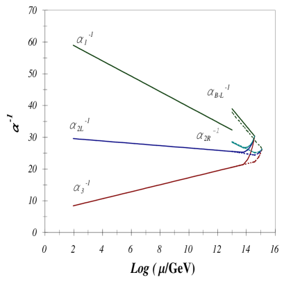
Figure 4: This figure shows the running of the the gauge couplings for the minimal supersymmetric left-right model in the presence of one extra dimension with all gauge fields in the bulk.

Reflections

This set of lectures is meant to be a pedagogical overview of the vast (and still expanding) field of supersymmetric grand unification- recently re-energised by ideas from strongly coupled string theories that bring in many new concepts and possibilities such as large extra dimensions, low string scales, bulk neutrinos etc. There are many unsolved problems not just of technical nature but of fundamental nature. The most glaring of the fundamental ones relating to string theories is of course how to stabilize the dilaton that is at the heart of the strong coupling discussion as well the discussion of unification and compactification. Among the thechnical ones are: construction of explicit string models that embody the “fantasies” scattered throughout the literature, before they faint away and evaporate in the glare of some other new ideas. It will involve a better understanding of internal string dynamics, a really challenging task since we dont seem to have a string field theory. Only after this huddle is surpassed, can we hope to bridge the big “disconnect” between string theories and the experiments that still makes many people uncomfortable to accept them as the final stage for the ultimate drama of physics. Meanwhile for those who wish to stay away from the hardships of string life have plenty to exercise their imagination- anything from finding a better solution to the doublet-triplet splitting to other phenomenological studies that can discrminate between different models.

Finally, an apology: the body of literature in this field is large and only a very selective sample has been given and this means that many important papers have not been cited. The ones cited should be consulted for additional references. It is hoped that this overview is of help in inspiring the reader to push the frontier in this extremely exciting field a bit further. Clearly, as it is stressed often here, there is an enormous amount that remains to be done and we are unlikely to see the final theory of everything anytime soon (a good thing too!), although progress in the last two decades has been enormous.

The author would like to thank G. Senjanović and A. Smirnov for organizing a pleasant summer school and creating an environment that promotes interaction between the students and the lecturers in such an effective manner. He is grateful to Howie Baer for a careful reading of the manuscript and suggestions. He would like to acknowledge the support from ICTP during the school and also take the opportunity to thank many students at the school for their comments. This work has been supported by the National Science Foundation grant no. PHY-9802551.

References

References

- [1] J Bagger, J Wess: Supersymmetry and Supergravity, Princeton University Press (1983).
- [2] R N Mohapatra: Unification and Supersymmetry, Springer-Verlag, Second edition (1991) and Supersymmetry, Supergravity and Supercolliders, TASI97, ed. J. Bagger (World Scientific, 1998), page 601.
- [3] H Haber, G Kane: Phys. Rep. 117, 76 (1984).
- [4] H P Nilles: Phys. Rep. 110, 1 (1984).
- [5] M Grisaru, M Rocek, W Siegel: Nucl. Phys. B159, 429 (1979).
- [6] Supersymmetry-96: Theoretical Perspectives and Experimental Outlook, ed. R N Mohapatra and A Rasin, North Holland (1997).
- [7] H. Haber, TASI lectures (1994); for a recent reviews see K. Dienes and C. Kolda, hep-ph/9712322; S. Martin, hep-ph/9709356.
- [8] S. Dawson, Supersymmetry, Supergravity and Supercolliders, TASI97, ed. J. Bagger (World Scientific, 1998).
- [9] R. Arnowitt, A. Chamseddine and P. Nath, Applied N=1 Supergravity, World Scientific (1984); R. Barbieri, S. Ferrara and C. Savoy, Phys. Lett. 119B, 343 (1982); J. Polonyi, Budapest preprint, KFK-1977-93 (1977).
- [10] M Dine, A Nelson: D 48, 1277 (1993); M. Dine, A.E. Nelson, Y. Nir, and Y. Shirman, hep-ph/9507378; Phys. Rev. D53 (1996) 2658; A.E. Nelson, hep-ph/9511218; M. Dine and A.E. Nelson, Phys. Rev. D48, 1277 (1993); M. Dine, A.E. Nelson, and Y. Shirman, Phys. Rev. D51, 1362 (1995).
- [11] P Binetruy, E Dudas, Phys. Lett. B389, 503 (1996); G Dvali, A Pomarol, Phys. Rev. lett. 77, 3728 (1996); R N Mohapatra, A Riotto, Phys. Rev. D55, 4262 (1997).
- [12] L. Randall and R. Sundrum, hep-th/9810155.
- [13] G. F. Giudice, M. A. Luty, H. Murayama and R. Rattazi, hep-ph/9810442.
- [14] Z. Chacko, M. Luty, I. Maksymik and E. Ponton, hep-ph/9905390; A. Pomarol and R. Rattazzi, hep-ph/9903448.
- [15] C. S. Aulakh and R. N. Mohapatra, Phys. Lett. 119B, 36 (1982); L. Hall and M. Suzuki, Nucl. Phys. B231, 419 (1984); V Barger, G F Giudice, M Y Han; Phys. Rev. 40, 2987 (1989); For a recent review, see G Bhattacharyya, Proceedings of SUSY’96, Nucl. Phys. (Proc. Suppl.), 52A, 83 (1996); H. Dreiner, hep-ph/9709356.
- [16] F. Gabbiani, E. Gabrielli, A. Masiero and L. Silvestrini, hep-ph/9604387.
- [17] For a review see R. Garisto, Nucl. Phys. B419, 279 (1994).
- [18] E. Cremmer, S. Ferrara, L. Girardello and A. van Proeyen, Nucl. Phys. B212, 413 (1983); J. Bagger, Nucl. Phys. B211, 302 (1983).
- [19] K. Inoue et al. Prog. Theor. Phys. 68, 927 (1982); L. Ibanez and G. Ross, Phys. Lett. B110, 227 (1982); L. Alvarez-gaume, J. Polchinski and M. Wise, Nucl. Phys. B250, 495 (1983).
- [20] For a review see, E. Cremmer, S. Ferrara, C. Kounas and D. V. Nanopoulos, Phys. Lett. 133B, 61 (1983).
- [21] E. Witten, Phys. Lett. 155B, 151 (1985).
- [22] R. N. Mohapatra and S. Nandi, Phys. Rev. Lett. 79, 181 (1997); Z. Chacko, B. Dutta, R. N. Mohapatra and S. Nandi, Phys. Rev. D 56, 5466 (1997).
- [23] S. Ambrosanio, G. Kane, G. Kribs, S. Martin and S. Mrenna, Phys. Rev. Lett. 76 (1996) 3498; S. Dimopoulos, M. Dine, S. Raby and S. Thomas, ibid 76 (1996) 3494; K. S. Babu, C. Kolda and F. Wilczek, hep-ph/9605408; S. P. Martin, hep-ph/9608224 ; G. Dvali, G. F. Giudice and A. Pomarol, hep-ph/9603238; A. Riotto, N. Tornquist and R. N. Mohapatra, Phys. Lett. B 388, 599 (1996); S. Dimopoulos, S. Thomas and J. Wells, hep-ph/9609434; J. Bagger, D. Pierce, K. Matchev and R.-J Zhang, hep-ph/9609443; E. Poppitz and S. Trivedi, hep-ph/9609529; I. Dasgupta, B. Dobrescu and L. Randall, hep-ph/9607487; H. Baer et al, hep-ph/9610358; A. de Gouvea, T. Moroi and H. Murayama, hep-ph/9701244; D. Dicus, B. Dutta and S. Nandi, hep-ph/9701341; N. Arkani-hamed, H. Murayama and J. March-Russell, hep-ph/9701286; G. Bhattacharyya and A. Romanino, hep-ph/9611243; S. Raby, Phys. Rev. D56, 2852 (1997); M. Luty, hep-ph/9706554.
- [24] M. Dine, N. Seiberg and E. Witten, Nucl. Phys. B289, 585 (1987); J. Attick, L. Dixon and A. Sen, ibid B292, 109 (1987).
- [25] G. Dvali and A. Pomarol, hep-ph9708304; Z. Berezhiani and Z. Tavartkiladze, Phys. Lett. B396, 150 (1997) and B409, 220 (1997); Ren-Jie Zhang, hep-ph/9702333; P. Binetruy, N. Irges, S. Lavignac and P. Ramond, hep-ph/9612442; N. Arkani- Hamed and H. Murayama, hep-ph/9703259; A. Nelson and D. Wright, hep-ph/9702359; A. Faraggi and J. C. Pati, hep-ph/9712516.
- [26] S Giddings, A Strominger, Nucl. Phys. B 307, 854 (1988).
- [27] R N Mohapatra: Phys. Rev. 34, 3457 (1986); A. Font, L. Ibanez and F. Quevedo, Phys. Lett. B228, 79 (1989); S. P. Martin, Phys. Rev. D46, 2769 (1992).
- [28] M. Gell-Mann, P. Ramond and R. Slansky, Supergravity, ed. D. Freedman and P. van Niuenhuizen (North Holland, 1979); T. Yanagida, KEK Lectures, (1979); R. N. Mohapatra and G. Senjanović, Phys. Rev. Lett. 44, 912 (1980).
- [29] R Kuchimanchi, R N Mohapatra: Phys. Rev. 48, 4352 (1993).
- [30] R. Kuchimanchi and R. N. Mohapatra, Phys. Rev. Lett. 75, 3989 (1995); C. Aulakh, K. Benakli and G. Senjanović, hep-ph/9703434; Phys. Rev. Lett. 79, 2188 (1997).
- [31] R. N. Mohapatra and A. Rasin, Phys. Rev. Lett. 76, 3490 (1996); C. S. Aulakh, A. Melfo and G. Senjanović, hep-ph/9707256; C. S. Aulakh, A. Melfo, A. Rasin and G. Senjanović, hep-ph/9712551.
- [32] Z. Chacko and R. N. Mohapatra, hep-ph/9712359.
- [33] R. N. Mohapatra and A. Rasin, Phys. Rev. D54, 5835 (1996).
- [34] R. N. Mohapatra and A. Rasin, Phys. Rev. Lett. 76, 3490 (1996); R. Kuchimanchi, Phys. Rev. Lett. 76, 3486 (1996); R. N. Mohapatra, A. Rasin and G. Senjanović, Phys. Rev. Lett. 79, 4744 (1997).
- [35] M. Pospelov, Phys. Lett. B391, 324 (1997).
- [36] K. S. Babu, B. Dutta and R. N. Mohapatra, hep-ph/9812421, hep-ph/9904366 and hep-ph/9905464.
- [37] C. Hamzoui and M. Pospelov, hep-ph/9803354.
- [38] M Francis, M Frank, C S Kalman, Phys. Rev. D 43, 2369 (1991); K Huitu, J Malaampi, M Raidal, Nucl. Phys. B 420, 449 (1994).
- [39] J. C. Pati and A. Salam, Phys. Rev. D10, 275 (1974).
- [40] H. Georgi and S. L. Glashow, Phys. Rev. Lett. 32, 438 (1974).
- [41] H. Georgi, H. Quinn and S. Weinberg, Phys. Rev. Lett. 33, 451 (1974).
- [42] W. Marciano and G. Senjanović, Phys. Rev. D25, 3092 (1982); U. Amaldi, W. de Boer and H. Furstenau, Phys. Lett. B260,447 (1991); P. Langacker and M. Luo, Phys. Rev. D44, 817 (1991); J. Ellis, S. kelly and D. Nanopoulos, Phys. Lett. B260, 131 (1991).
- [43] D. Chang, R. N. Mohapatra, M. K. Parida, J. Gipson and R. E. Marshak, Phys. Rev. D31, 1718 (1985); N. G. Deshpanda, E. Keith and P. Pal, Phys. Rev. D46, 2261 (1992); R. N. Mohapatra and M. K. Parida, Phys. Rev. D 47, 264 (1993); F. Acampora, G. Amelino-Camelia, F. Buccella, O. Pisanti, L. Rosa and T. Tuzi, DSF preprint 93/52.
- [44] B. Brahmachari and R. N. Mohapatra, Int. Journ. Mod. Phys. A 11, 1699 (1996).
- [45] M. Schmelling, hep-ex/9701002.
- [46] Many papers have addressed this issue; see for instance, M. Bastero-gil and J. Perez-Mercader, Nucl. Phys. B450, 21 (1995); P. Langacker and N. Polonsky, Phys. Rev. D 52, 3081 (1995).
- [47] J. Bagger, K. Matchev, D. Pierce and R. J. Zhang, hep-ph/9611229 and hep-ph/9606211.
- [48] M. Olechowski and S. Pokorski, Phys. Lett. B214, 393 (1988); B. Ananthanarayan, G. Lazaridis and Q. Shafi, Phys. Rev. D 44, 1613 (1991); R. Rattazi, U. Sarid and L. Hall, hep-ph/9405313.
- [49] V. Barger, M. Berger, T. Han and M. Zralek, Phys. Rev. Lett. 68, 3894 (1992).
- [50] C. Hill, Phys. Rev. D24, 691 (1981); C. Penddleton and G. Ross, Phys. Lett. B98, 291 (1981).
- [51] H. Baer, M. Diaz, J. Ferrandis and X. Tata, Phys. Rev. D61, 111701 (2000); H. Baer, M. Brhlik, M. A. Diaz and X. Tata, hep-ph/0005027.
- [52] S. Dimopoulos and H. Georgi, Nucl. Phys. B193, 150 (1981); N. Sakai, Z. Phys. C11, 153 (1981).
- [53] R. Arnowitt, A. Chamsheddine and P. Nath, Phys. Lett. B156, 215 (1985).
- [54] For a review see, R. Arnowitt and P. Nath, Lectures at the VII J. Swieca Summer school, 1993, CTP-TAMU-52/93.
- [55] R. Barbieri, Z. Berezhiani and A. Strumia, hep-ph/9704275.
- [56] V. Kuzmin, V. Rubakov and M. Shaposnikov, Phys. Lett. B155, 36 (1985); for a review and other references, see A. Cohen, D. Kaplan and A. Nelson, Ann. Rev. Nucl. Sc. 43, 27 (1993).
- [57] R. N. Mohapatra and B. Sakita, Phys. Rev. D21, 1062 (1980).
- [58] For an alternative formulation see, F. Wilczek and A. Zee, Phys. Rev. D25, 553 (1982).
- [59] D. Chang, R. N. Mohapatra and M. K. Parida, Phys. Rev. Lett. 52, 1072 (1974).
- [60] T. Kibble, G. Lazaridis and Q. Shafi, Phys. Rev. D26, 435 (1982).
- [61] H. Georgi and C. Jarlskog, Phys. Lett. B86, 297 (1979).
- [62] J. Harvey, P. Ramond and D. Reiss, Phys. Lett. 92B, 309 (1980); X. G. He and S. Meljanac, Phys. Rev. D41, 1620 (1990); S. Dimopoulos L. Hall and S. Raby, Phys. Rev. Lett. 68, 1984 (1992); K. S. Babu and R. N. Mohapatra, Phys. Rev. Lett. 74, 2418 (1995).
- [63] R. N. Mohapatra and P. B. Pal, Massive neutrinos in Physics and Astrophysics, (World Scientific, 1989).
- [64] K. Dienes, Phys. Rep. 287, 447 (1997); K. Dienes and J. March-Russel, hep-th/9604112; see however, J. Erler, Nucl. Phys. B475, 597 (1996) where it is argued one may get 126’s in more general string compactifications.
- [65] S. Choudhuri, S. Chung and J. Lykken, hep-ph/9511456; G. Cleaver,hep-th/9708023; S. Choudhuri, S. Chung, G. Hockney and J. Lykken, Nucl. Phys. 456, 89 (1995); G. Aldazabal, A. Font, L. Ibanez and A. M. Uranga, Nucl. Phys. B452, 3 (1995).
- [66] K. S.Babu and S. Barr, Phys. Rev. D50, 3529 (1994); K. S. Babu and R. N. Mohapatra, Phys. Rev. Lett. 74, 2418 (1995); L. Hall and S. Raby, Phys. Rev. D51, 6524 (1995); D. G. Lee and R. N. Mohapatra, Phys. Rev. D51, 1353 (1995); S. Barr and S. Raby, hep-ph/9705366; C. Albright and S. Barr, hep-ph/9712488; Z. Berezhiani, Phys. Lett. B355, 178 (1995).
- [67] R. N. Mohapatra, Phys. Rev. Lett. 56, 561 (1986); R. N. Mohapatra and J. W. F. Valle, Phys. Rev. D34, 1642 (1986).
- [68] S. Dimopoulos and F. Wilczek, I.T.P preprint (unpublished); K. S. Babu and S. Barr, Phys. Rev. D48, 5354 (1993).
- [69] D. G. Lee and R. N. Mohapatra, Phys. Rev. D51, 1353 (1995).
- [70] K. S. Babu and R. N. Mohapatra, Phys. Rev. Lett. 74, 2418 (1995).
- [71] Z. Chacko and R. N. Mohapatra, Phys. Rev. Lett. 82, 2836 (1999); G. Dvali and S. Pokorski, Phys. Lett. B379, 126 (1996).
- [72] M. Fukugita and T. Yanagida, Phys. Lett. B174, 45 (1986).
- [73] T. Gherghetta and G. Jungman, Phys. Rev. D 48, 1543 (1993); W. Buchmuller and M. Plumacher, hep-ph/9711208.
- [74] F. Gursey and P. Sikivie, 36, 775 (1976); P. Ramond, Nucl. Phys.B 110, 224 (1976).
- [75] For a review of these developments, see M. Green, J. Schwarz and E. Witten, Superstring Theories, (Cambridge University Press, 1989).
- [76] G. Altarelli, hep-ph/9710434.
- [77] A. Davidson and K. C. Wali, Phys. Rev. Lett. 58, 2623 (1987); Peter Cho, Phys. Rev. D48, 5331 (1993).
- [78] R. N. Mohapatra, Phys. Lett. B379, 115 (1996).
- [79] I. Antoniadis, J. Ellis, J. Hagelin and D. Nanopoulos, Phys. Lett. B 231, 65 (1989); J. Lopez, D. V. Nanopoulos and K. Yuan, Nucl. Phys. B399, 654 (1993).
- [80] Z. Berezhiani and G. Dvali, Sov. Phys. Leb. Inst. Rep. 5, 55 (1989).
- [81] Z. Berezhiani, L. Randall and C. Csaki, Nucl. Phys. B444, 61 (1995); Z. Berezhiani, Phys. Lett. B355, 481 (1995); R. Barbieri, Nucl. Phys. B432, 49 (1994); G. Dvali and S. Pokorski, hep-ph/9610341.
- [82] L. Hall, V. Kostelecky and S. Raby, Nucl. Phys. B267, 415 (1986); R. Barbieri and L. Hall, Phys. Lett. B338, 212 (1994); N. G. Deshpande, B. Dutta and E. Keith, OITS-595; T. V. Duong, B. Dutta and E. Keith, hep-ph/9510441; H. Goldberg and M. Gomez, Phys. Rev. D 53, 5244 (1996).
- [83] H. Walter, Talk at the conference on Lepton Moments, Heidelberg (1999).
- [84] B. Balakrishna, A. Kagan and R. N. Mohapatra, Phys. Lett. 205B, 345 (1988); For a review, see K. S. Babu and E. Ma, Mod. Phys. Lett. A4, 1975 (1989).
- [85] For a review, see K. Dienes, Phys. Rep. 287, 447 (1997).
- [86] P. Ginsparg, Phys. Lett. 197, 139 (1987).
- [87] P. Candelas, G. Horowitz, A. Strominger and E. Witten, Nucl. Phys. B 258, 46 (1985).
- [88] P. Horava and E. Witten, Nucl. Phys. B 460, 506 (1996).
- [89] For a review, see H. P. Nilles, Supersymmetry, Supergravity and Supercolliders, TASI97, ed. J. Bagger (World Scientific, 1998).
- [90] J. Lykken, Phys. Rev. D 54, 3693 (1996).
- [91] I. Antoniadis, Phys. Lett. B 246, 377 (1990); I. Antoniadis, K. Benakli and M. Quirós, Phys. Lett. B331,313 (1994).
- [92] N. Arkani-Hamed, S. Dimopoulos and G. Dvali, Phys. Lett. B429 (1998) 263; Phys. Rev. D59, 086004 (1999); I. Antoniadis, S. Dimopoulos and G. Dvali, Nucl. Phys. B 516, 70 (1998); N. Arkani-hamed, S. Dimopoulos and J. March-Russell, hep-th/9809124.
- [93] G. Giudice, R. Rattazzi and J. Wells, Nucl. Phys. B 544,3 (1999); E. Mirabelli, M. Perelstein and M. Peskin, hep-ph/9811337; T. Han, J. Lykken and R. J. Zhang, hep-ph/9811350; J. L. Hewett, hep-ph/9811356; P. Mathew, K. Sridhar and S. Raichoudhuri, hep-ph/9811501; T. G. Rizzo, hep-ph/9901209; K. Aghase and N. G. Deshpande, hep-ph/9902263; K. Cheung and W. Y. Keung, hep-ph/9903294.
- [94] K.R. Dienes, E. Dudas and T. Gherghetta, Phys. Lett. B436, 55 (1998) ; Nucl. Phys. B537, 47 (1999); for an earlier discussion see T. Taylor and G. Veneziano, Phys. Lett. B212, 147 (1988).
- [95] A. Perez-Lorenzana and R. N. Mohapatra, hep-ph/9904504.
- [96] D. Ghilencea and G.G. Ross, Phys. Lett. B442, 165 (1998); Z. Kakushadze, hep-ph/9811193; C.D. Carone, hep-ph/9902407; A. Delgado and M. Quirós, hep-ph/9903400; P. H. Frampton and A. Rǎsin, hep-ph/9903479; D. Dumitru and S. Nandi, hep-ph/9906514.
- [97] K. Dienes, E. Dudas and A. Gherghetta, hep-ph/9811 428; N. Arkani-Hamed, S. Dimopoulos, G. Dvali and J. March-Russell, hep-ph/9811448; G. Dvali and A. Smirnov, hep-ph/9904211.
- [98] R. N. Mohapatra, S. Nandi and A. Perez-Lorenzana, hep-ph/9907520; R. N. Mohapatra and A. Perez-Lorenzana, hep-ph/9910474.