Abstract

The well-known Monte Carlo simulation packet JETSET is not built in order to describe few-body states (in particular at the few GeV level in $e^{+}e^{-}$ annihilation as in BEPC). In this note we will develop the formalism to use the basic Lund Model area law directly for Monte Carlo simulations.

1 Introduction

The Lund Fragmentation Model contains a set of simple assumptions. Based upon them one obtains as a final result an area law for the production of a set of mesons from a string-like force field. It is possible to reformulate this into an iterative cascade process in which one particle is produced at a time. This is essentially the way the model is implemented in the JETSET Monte Carlo packet${}^{\cite[cite]{[\@@bibref{}{TS}{}{}]}}$.

In all computer programs it is necessary to make certain approximations, but the approximations in JETSET are hardly noticeable against the background noise signals as soon as sufficiently many particles are produced. For the few-body states (in particular at low energies) this is, however, no longer the case and in order to treat these situations it is necessary to use other means to implement the Lund Model as a Monte Carlo simulation program. In this note we will show how to make use of the basic area-law directly. We will be satisfied to treat two-body up to six-body states, which constitutes the overwhelming amount of the data obtained at the BEPC/BES accelerator in Beijing.

We will start by briefly reviewing some features of the string fragmentation scheme in the Lund Model. After that we will in the next section show how to implement the basic area law and present the Monte Carlo program LUARLW. Finally we will show some results, in particular point to some places where there are major deviations between the results from JETSET and LUARLW.

Although the formulas in the Lund Model are derived${}^{\cite[cite]{[\@@bibref{}{BoSBAGG}{}{}]}}$, using (semi-)classical probabilities the final results can by comparison to different quantum mechanical processes be extended outside this framework${}^{\cite[cite]{[\@@bibref{}{BA}{}{}]}}$. We will in this paper neglect all gluonic emissions and concentrate on the situation when the (color) force field from an original quark($q_{0}$)-antiquark($\bar{q}_{0}$) pair, produced in e.g. an $e^{+}e^{-}$ annihilation event, decays into a set of final state hadrons. These are usually termed two-jet events. The transverse momentum of the final state particles will be treated in accordance with a tunneling process, which leads to gaussian transverse fluctuations, which are governed by the strength of the string constant $\kappa$.

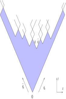
Figure 1: String fragmentation and mesons production in $t-x$ space

The color force fields are in the Lund Model modeled by the massless relativistic string with color $3$($q$) and $\bar{3}$($\bar{q}$) at the endpoints (the gluons ($g$, color$8$) are treated as internal excitations on the string field). This means that there is a constant force field ($\kappa\simeq 1~{}GeV/fm$, corresponding to a linearly rising potential) spanned between the original pair. This pair is produced at the origin $O$, cf. Fig.1, and afterwards the $(q_{0}\bar{q}_{0})$ are moving apart along the $x$-axis (the longitudinal direction). The energy in the field can be used to produce new $q\bar{q}$-pairs (new endpoints, thereby breaking the string). The production rate of such a pair (mass(es) $\mu$, transverse momentum $\pm{\bf k}_{\perp}$, transverse mass(es) $\mu_{\perp}=\sqrt{\mu^{2}+{\bf k}_{\perp}^{2}}$ and with combined internal quantum numbers corresponding to the vacuum) is from quantum mechanical tunneling in a constant force field equal to

$$\exp\left(-\frac{\pi\mu_{\perp}^{2}}{\kappa}\right).$$ (1)

The final state mesons in the Lund Model correspond to isolated string pieces containing a $q$ from one breakup point (vertex) and a $\bar{q}$ from the adjacent vertex together with the produced transverse momentum and the field energy in between.

In order to simplify the formulas and the pictures we will treat all $q\bar{q}$-particles as massless and therefore as moving along light-cones (massive $q\bar{q}$-particles move in this semi-classical scenario along hyperbolas with these light-cones as asymptotes but the final results are the same${}^{\cite[cite]{[\@@bibref{}{BA}{}{}]}}$). For the longitudinal dynamics in the Lund Model this is in accordance with quantum mechanics (in practice we only use dynamical features where position and rapidity of the particles are the relevant variables and this is allowed by the indeterminacy relations${}^{\cite[cite]{[\@@bibref{}{GottLow}{}{}]}}$).

One necessary requirement is that to obtain real positive (transverse) masses all the vertices must have spacelike difference vectors. Together with Lorentz invariance this means that all the vertices in the production process must be treated in the same way${}^{\cite[cite]{[\@@bibref{}{BoSBAGG}{}{}]}}$. Another consequence is that it is always the slowest mesons that are firstly produced in any Lorentz frame (corresponding to the fact that time-ordering is frame dependent; this is also in accordance with the well-known Landau-Pomeranchuk formation time concept). Further each vertex has the property, cf. Fig. 1, that it will divide the event into two jets; the mesons produced along the string field to the right and those produced to the left of the vertex. This feature implies that it is consistent to introduce a rank-ordering along the light-cones so that the first rank particle contains the original $q_{0}$ (or $\bar{q}_{0}$) together with the $\bar{q}$ ($q$) produced at the first vertex etc. Whether the process is ordered along one or another of the light-cones should be irrelevant.

Based upon these assumptions it is possible to obtain a unique stochastical process for the decay ${}^{\cite[cite]{[\@@bibref{}{BoSBAGG}{}{}]},\cite[cite]{[\@@bibref{}{BA}{}{}]}}$. In particular this process will turn out to have simple factorization properties so that for every finite energy, rank-connected group of final state particles (which may possibly be part of the result from a large or even infinitely large energy reaction) there is a factor corresponding to the probability to produce the cluster with a certain energy and another corresponding to the probability that it decays into just this particular final state. We will from now on concentrate on this latter probability distribution.

We find that the (non-normalized) probability for the cluster to decay into the particular channel with the $n$ particles $\{p_{j}\}$ is given by

$$dP_{int}=[\prod\limits_{j=1}^{n}N_{j}d^{2}p_{j}]\delta(p_{j}^{2}-m_{j}^{2})\delta(\sum\limits_{j=1}^{n}p_{j}-P_{tot})\exp(-b{\cal A}).$$ (2)

We note the appearance of the phase space for the final state particles multiplied by the exponential area (${\cal A}$ is the shadow region in Fig. 1) decay law. The quantity $P_{tot}$ is the total energy momentum of the cluster so that $P_{tot}^{2}=s$, $b$ is a fundamental color-dynamical parameter and $N_{j}$ are normalization constants. Actually it is possible to generalize this result and include some special vertex factors but just as it is in connection with JETSET we have found no necessity to use such generalizations for the results in this paper.

We will start the investigation assuming that there is a single particle species with mass $m$. Due to Lorentz invariance the integral of the distribution $dP_{int}$ can only depend upon $s$ and this means that we can define the function $R_{n}$ for the multiplicity $n$ by

$$\int dP_{int}(p_{1},\cdots,p_{n})=R_{n}(s).$$ (3)

It is possible to subdivide these integrals into one part, that will depend solely upon the first-rank particle $p_{1}$ and a remainder part. The phase space element can be written as $dp_{1}\delta(p_{1}^{2}-m_{1}^{2})=dz_{1}/z_{1}$ with $p_{+1}=z_{1}P_{+tot}$ and $p_{-1}=m_{1}^{2}/p_{+1}$. Similarly we find for the area

$${\cal A}(1,\cdots n)=m_{1}^{2}/z_{1}+{\cal A}(2,\cdots n).$$ (4)

Finally the energy momentum $P_{1}$, obtained after taking away the first particle, fulfills

$$(P_{1})^{2}\equiv s_{1}=(P_{tot}-p_{1})^{2}=(1-z_{1})(s-m_{1}^{2}/z_{1}).$$ (5)

Therefore we obtain an integral equation linking $R_{n}$ to $R_{n-1}$:

$$R_{n}(s)=\int N_{1}\frac{dz_{1}}{z_{1}}\exp(-bm_{1}^{2}/z_{1})R_{n-1}(s_{1}).$$ (6)

If we define the function $R(s)=\sum\limits_{n}R_{n}(s)$ the Eq (6) will be valid also for $R$ itself (to be precise there is a lower cutoff in $z$ to make it possible to produce more than one particle). The equation has an (asymptotic) solution $R\propto s^{a}$ if

$$1=\int N_{1}\frac{dz}{z}(1-z)^{a}\exp(-bm_{1}^{2})\equiv\int f(z)dz.$$ (7)

We have neglected a finite energy correction term $(1-m_{1}^{2}/zs)^{a}$ in the asymptotic limit. This defines the fragmentation function $f$ in the Lund Model and this is the way JETSET implements the model.

To be more precise, JETSET contains the production of all known particles. It is assumed that the parameters $b$ and $a$ are fixed by experiments (ordinary default values in the LEP region are $b\simeq 0.6$ $GeV^{-2}$ and $a\simeq 0.3-0.5$) and that $N_{j}$ normalizes the fragmentation function for each given mass $m_{j}$. The relative probability of the different particle flavors is decided by an external procedure. Thus the production of strange quark-pairs ($s\bar{s}$) are suppressed compared to $u$ and $d$ (cf. Eq.(1), an ordinary default value for the suppression factor is $0.3$). It is further assumed (and this can be verified on a qualitative level) that it should be more difficult for a quark to tunnel into a vector meson (tensor meson) state (in the string model essentially a one-dimensional bag) than into a pseudoscalar state. For the production of baryons there are several more parameters (and recent investigations${}^{\cite[cite]{[\@@bibref{}{PEGG}{}{}]}}$ indicates that for a description of baryon production one needs to introduce special features).

There is another possible interpretation which has been pursued by a group from UCLA${}^{\cite[cite]{[\@@bibref{}{CDB}{}{}]}}$. In that case all the numbers $b$, $a$ and $N$ are taken as experimentally determinable parameters and the size of the fragmentation function integral in Eq. (7) is used to determine the relative weight for the production of different particles. They use some straightforward Clebsch-Gordan coefficients, take into account that strangeness and baryon number must be conserved (thus e.g. the production of pairs of strange mesons must be used to determine the relative weight) etc. and with very few parameters they seem to obtain a phenomenologically good fit to data.

There is, however, in both these implementations the problem of how to end the cascade process. In JETSET (and UCLA is using a similar procedure) the process is pursued stochastically from both endpoints and continues until there is a remainder mass of a certain size. This remainder is then fragmented as a two-particle state. This “joining”-procedure is implemented with great care in JETSET but nevertheless provides some unwanted features in particular for few-body states and low energies which is the main subject of this note. In the next section we will present a different procedure.

2 Formalism

Our basic assumption will be that the area-law, supplemented with certain simple probabilities similar to JETSET, will be fundamental also for low-energy and few-body states. We will further use a gaussian transverse momentum spectrum and the procedure is outlined in Appendix 1. We will for definiteness order the particles in rank along the positive light-cone.

A particularly simple case is the two-body decay because in this case energy-momentum conservation determines all the observables. We obtain immediately for the quantity $R_{2}$ (using $m_{j}$, $j=1,2$, for the transverse masses; note that transverse momentum conservation in this case implies that ${\bf p}_{\perp 1}=-{\bf p}_{\perp 2}$)

$$R_{2}=N_{1}N_{2}\frac{2exp[-\frac{b}{2}(s+m^{2}_{1}+m_{2}^{2})]}{\sqrt{\lambda(s,m_{1}^{2},m_{2}^{2})}}\cosh(\sqrt{\lambda(s,m_{1}^{2},m_{2}^{2})}~{}),$$ (8)

where the $\lambda$ is defined as

$$\lambda(x,y,z)=x^{2}+y^{2}+z^{2}-2xy-2xz-2yz.$$

The two different terms correspond to the two different values that can be chosen for the positive light-cone fraction $z_{j}=p_{+j}/P_{+}$

$$z_{1}^{\pm} = \frac{s+m_{1}^{2}-m_{2}^{2}\pm\sqrt{\lambda(s,m_{1}^{2},m_{2}^{2})}}{2s},$$

$$z_{2}^{\pm} = \frac{s+m_{2}^{2}-m_{1}^{2}\mp\sqrt{\lambda(s,m_{1}^{2},m_{2}^{2})}}{2s}.$$ (9)

We note that the two solutions will fulfill the relation $z_{j}^{+}z_{j}^{-}s=m_{j}^{2}$. This evidently means that we obtain the corresponding negative light-cone fractions by exchanging the sign in front of the square root. Although the expression for $R_{2}$ looks singular at the threshold $\sqrt{s}=m_{1}+m_{2}$, it is in practice finite and even vanishing if the transverse momentum fluctuations are taken into account.

From the expression for $R_{2}$ we may derive the expression for $R_{3}$ according to Eq. (6) but it is actually more convenient to consider $R_{3}$ as a density in the area-size ${\cal A}_{3}$. Again using the positive light-cone fractions $z_{j}$ ($j=1,2,3$) we may write the energy-momentum conservation equations and the size of ${\cal A}$ as

$$\sum\limits_{j=1}^{3}z_{j}=1,$$

$$\sum\limits_{j=1}^{3}\frac{m_{j}^{2}}{z_{j}}=s,$$

$$\frac{m_{1}^{2}}{z_{1}}+\frac{m_{2}^{2}}{z_{2}}(1-z_{1})+m_{3}^{2}={\cal A}.$$ (10)

Performing the integral we obtain

$$dR_{3}=\prod\limits_{j=1}^{3}N_{j}\frac{\exp(-b{\cal A})d{\cal A}}{\sqrt{\Lambda}},$$ (11)

where,

$$\Lambda = [(s-{\cal A})({\cal A}-m_{\perp 1}^{2}-m_{\perp 2}^{2}-m_{\perp 3}^{2})$$

$$- m_{\perp 1}^{2}m_{\perp 2}^{2}-m_{\perp 2}^{2}m_{\perp 3}^{2}-m_{\perp 3}^{2}m_{\perp 1}^{2}]^{2}-4sm_{\perp 1}^{2}m_{\perp 2}^{2}m_{\perp 3}^{2}.$$

A closer investigation tells us that the area ${\cal A}$ in this three-body case will be limited to the region

$${\cal A}_{3}^{-} \leq {\cal A}~{}\leq~{}{\cal A}_{3}^{+},$$

$${\cal A}_{3}^{\pm} = \frac{s+U\pm\sqrt{(s-U)^{2}-4(V+\sqrt{W})}}{2},$$ (12)

and that the quantity $\Lambda$ can be written as

$$\Lambda=({\cal A}_{3}^{+}-{\cal A})({\cal A}-{\cal A}_{3}^{-})[(s-{\cal A})({\cal A}-U)-V+\sqrt{W}),$$ (13)

where we have introduced the notations

$$U = m_{1}^{2}+m_{2}^{2}+m_{3}^{2},$$

$$V = m_{1}^{2}m_{2}^{2}+m_{2}^{2}m_{3}^{2}+m_{3}^{2}m_{1}^{2},$$

$$W = 4sm_{1}^{2}m_{2}^{2}m_{3}^{2}.$$

In this way the limits on the area corresponds to two of the zeros of the quantity $\Lambda$. It is rather easy to see that the particle configurations corresponding to ${\cal A}={\cal A}_{3}^{\pm}$ corresponds to the cases when the vertices (the breakup points) both lie on the same hyperbola. This means in particular that all the possible areas for the three-body decay are in between the two hyperbolas. To see that it is useful to note that the square root in the definition of ${\cal A}_{3}^{\pm}$ can be factorized as

$$(s-U)^{2}-4(V+\sqrt{W}) = [\sqrt{s}-m_{1}-m_{2}-m_{3}][\sqrt{s}+m_{1}+m_{2}-m_{3}]$$ (14)

$$\times [\sqrt{s}+m_{1}-m_{2}+m_{3}2][\sqrt{s}-m_{1}+m_{2}+m_{3}]$$

and that it is a direct generalization of the corresponding expression for the two-body distribution

$$\lambda(s,m_{1}^{2},m_{2}^{2})=[\sqrt{s}-m_{1}-m_{2}][\sqrt{s}+m_{1}+m_{2}][\sqrt{s}+m_{1}-m_{2}][\sqrt{s}-m_{1}+m_{2}].$$ (15)

There are two sets of solutions for the light-cone fractions for given masses, energy and area size ${\cal A}$ (just as for the two body case). They can be written as

$$z_{1}=\frac{-B\pm\sqrt{\Lambda}}{2s(A-m_{\perp 2}^{2}-m_{\perp 3}^{2})},$$ (16)

where,

$$B = A(A-m_{\perp 1}^{2}-m_{\perp 2}^{2}-m_{\perp 3}^{2})-s(A+m_{\perp 1}^{2}-m_{\perp 2}^{2}-m_{\perp 3}^{2})$$ (17)

$$+ m_{\perp 1}^{2}m_{\perp 2}^{2}+m_{\perp 2}^{2}m_{\perp 3}^{2}+m_{\perp 3}^{2}m_{\perp 1}^{2},$$

the corresponding values of $z_{2}$ and $z_{3}$ can be read out from Eqs. (2).

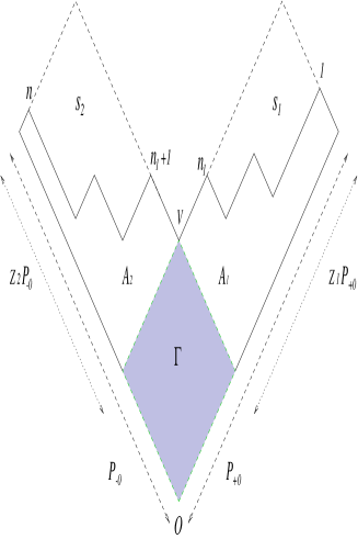
Figure 2: The vertex $V$ divides the system into two subsystems of “right-movers” (mesons $1,\cdots,n_{1}$) and “left-movers” (mesons $n_{1}+1,\cdots,n$).

For the general $n$-body case we have to generate the kinematical variables by means of an $(n-2)$-dimensional density but as we are going to limit ourselves to at most six particles we will make use of a different method. We will then for the four-body, five-body and six-body cases subdivide the system into two parts, each containing $n_{1}$ and $n_{2}$ particles ($n_{1},n_{2}=2$ or $3$ and $n=n_{1}+n_{2}$) . We may then, using the simple factorization properties of the model, apply the analytical results obtained above for the two parts.

In more detail the subsystem closest to the positive light-cone (the $q$-end of the string) will be characterized by the positive light-cone fraction $Z_{+}^{(1)}\equiv Z_{1}$ and the other subsystem by the (negative) light-cone fraction $Z_{-}^{(2)}\equiv Z_{2}$, cf. Fig.2. Then the squred invariant masses of the two systems are

$$s_{1}=Z_{1}(1-Z_{2})s {\rm and} s_{2}=Z_{2}(1-Z_{1})s,$$ (18)

the area can similarly be subdivided into

$$A=A_{1}+A_{2}+\Gamma {\rm with} \Gamma=(1-Z_{1})(1-Z_{2})s.$$ (19)

In this way we obtain immediately for $dR_{n}$ the result

$$dR_{n}=\frac{ds_{1}ds_{2}}{\sqrt{\lambda(s,s_{1},s_{2})}}[exp(-b\Gamma_{+})+exp(-b\Gamma_{-})]dR_{n_{1}}dR_{n_{2}}$$ (20)

in terms of the two possible $\Gamma$ values

$$\Gamma_{\pm}=[s-s_{1}+s_{2}\pm\sqrt{\lambda(s,s_{1},s_{2})}~{}][s-s_{2}+s_{1}\mp\sqrt{\lambda(s,s_{1},s_{2})}~{}]/4s.$$ (21)

The corresponding values for the $Z_{j}$ are (cf. the remarks after Eq. (2))

$$Z_{1}^{\pm} = [s-s_{2}+s_{1}\pm\sqrt{\lambda(s,s_{1},s_{2})}~{}]/2s,$$

$$Z_{2}^{\pm} = [s-s_{1}+s_{2}\mp\sqrt{\lambda(s,s_{1},s_{2})}~{}]/2s.$$ (22)

We note that the momentum and energies of the two subsystems as well as their c.m.s-rapidities are easily expressed in these variables. Consequently the whole events can be determined in a straightforward way as soon as the (transverse) masses and the c.m.s energy is given. It is, however, necessary to introduce a method to chose the flavors of the different particles.

We will use a method “in-between” the JETSET and the UCLA implementations and in particular normalize our results at the c.m.s-energy $\sqrt{s}=4$ $GeV$ to the JETSET ones. Thus we will assume that the probability to obtain a particular state with the $n$ mesons labeled $\{m_{j}\}$ (using the masses to characterize the particles) is given by

$$P_{n}(m_{1},\cdots,m_{n};s)=C(VPS)(SUD)N^{n}R_{n}(m_{1},\cdots,m_{n};s).$$ (23)

It turns out that the functions $R_{n}$ are the same independent of the rank-ordering of the particles. The quantity $C$ is then introduced as a combinatorial number (stemming from the quark contents of the possible strings-there are in general more than one such ordered “quark-string” possible to make the particular mesons and even sometimes the possibility to make the same meson(s) at different places in the same string). The quantities $(VPS)$ are the vector to pseudoscalar rate (we neglect the tensor mesons, although they can be introduced by straightforward means). The parameter $(SUD)$ is the strange to up and down $(q\bar{q})$ probability. It comes without saying that both $(VPS)$ and $(SUD)$ depends upon the number of choices to be made. The possibility to produce charm in the fragmentation process is-just as in JETSET- neglected in accordance with the results from Eq. (1). Finally $N$ is a parameter to obtain the right multiplicity distribution. To obtain the right multiplicity distribution we will sum over all the different orderings and strings in Eq. (23). In this way we find a default value for the parameter $N$ by comparison to JETSET.

The procedure to produce a state is then that we firstly chose the multiplicity from the sum over all the $R_{n}$ and then the particular state by a stochastical choice among the possible $n$-particle channels. After that we chose the particular ordering of the particles stochastically from the ways they can be produced from the possible quark-strings. Finally to obtain the particle distributions we just differentiate $R_{n}$ in the ways we have described it above.

In this way we have defined a simple few-body low-energy version of the Lund Model (although an incorporation of baryons into the scheme may have some influence upon the results). It is implemented in the Monte Carlo simulation program LUARLW${}^{\cite[cite]{[\@@bibref{}{HaimingHu}{}{}]}}$. A list of the default parameters of the model is given in Appendix 2.

3 Some Results of the Model

We will in this section exhibit a few results from the model implemented in the simulation program LUARLW, in particular discuss some configurations where the use of JETSET may be misleading in the few-body, low-energy cases.

We firstly note that in a model of iterative character it is in general difficult to obtain the right behavior for small relative rapidities between two (rank-connected) particles. To see that we consider such a two-particle state, that is a part of a larger system, and assume that the pair has a total (transverse) mass-square $s_{12}=m_{1}^{2}+m_{2}^{2}+2m_{1}m_{2}\cosh(\delta y)$ with $m_{j}$ the individual (transverse) masses and $\delta y$ the rapidity difference. This means that the distribution in $\delta y$ is

$$\frac{dP}{d\delta y}=\frac{dP}{ds_{12}}2m_{1}m_{2}\sinh(\delta y)$$ (24)

Therefore unless the distribution in $s_{12}$ behaves (for values of $\sqrt{s_{12}}$ close to $m_{1}+m_{2}$, i.e. for small $\delta y$) as $1/\sqrt{\lambda(s_{12},m_{1}^{2},m_{2}^{2})}=1/2m_{1}m_{2}\sinh(\delta y)$ then $dP/d\delta y$ will vanish. From the results discussed above this is in general taken into account by the generation mechanism in LUARLW but it is not so if we consider the corresponding situation in JETSET (cf. Fig. 3 and Fig.4). On the other hand it is difficult to observe this effect in a multi-particle environment so it is only for the few-body case it is of interest, especially if the phase space is small (low energies).

There is further the “joining mechanism” in JETSET and related simulation programs. One place where this is noticeable is if we consider the rapidity ordering of a particular set of particles as they are generated in LUARLW and in JETSET. As examples we have chosen the four-body states $\rho^{+}\rho^{-}\pi^{+}\pi^{-}$ and $K^{+}K^{-}\pi^{+}\pi^{-}$. In Table 1 we present the probabilities for the different possible orderings in two systems.

We have only pinpointed a few particular places where it may be possible to see the precise workings of the area-law as compared to an iterative production mechanism. We find several places where there are clear differences but our major finding is that it quite surprising how well the basic JETSET scenarium really works at such low energies and multiplicities.

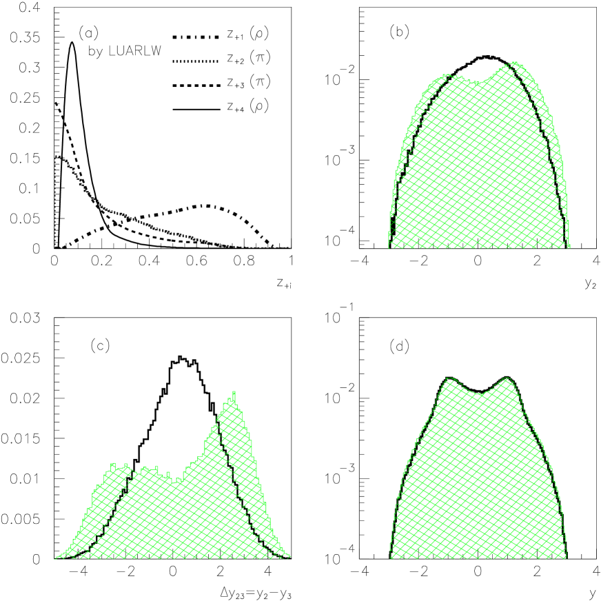
Figure 3: The light-cone component and rapidity distributions of a $\rho\pi\pi\rho$ final state at $\sqrt{s}=4~{}GeV$ (the ordering corresponds to rank-ordering). The distributions for the corresponding rank particle in JETSET (the net-like regions) and LUARLW (the solid lines) show significant differences, while the total inclusive distributions agree. The rapidity-difference in JETSET shows the gap near $\Delta y_{ij}\sim 0$ (the so-called “disease” distribution). Figure (a) is non-normalized.

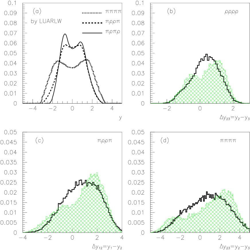
Figure 4: The distributions of rapidity and rapidity differences for some special final states at $\sqrt{s}=4~{}GeV$ predicted by JETSET (the net-like regions) and LUARLW (the solid lines).

final state	$\rho^{+}\rho^{-}\pi^{+}\pi^{-}$	$K^{+}K^{-}\pi^{+}\pi^{-}$
rapidity order	JETSET LUARLW	JETSET LUARLW
$y_{1}>y_{2}>y_{3}>y_{4}$	13.15   19.78	18.55   23.10
$y_{1}>y_{2}>y_{4}>y_{3}$	12.85   12.39	14.76   12.85
$y_{2}>y_{1}>y_{3}>y_{4}$	12.60   11.94	14.70   12.42
$y_{2}>y_{1}>y_{4}>y_{3}$	12.39    8.79	8.47     8.86
$y_{1}>y_{3}>y_{2}>y_{4}$	11.46    12.43	12.90   12.82
$y_{1}>y_{3}>y_{4}>y_{2}$	5.98     5.89	3.72     4.98
$y_{3}>y_{1}>y_{2}>y_{4}$	5.96     5.96	3.77     4.83
$y_{2}>y_{3}>y_{1}>y_{4}$	5.29     4.72	6.67     4.46
$y_{1}>y_{4}>y_{2}>y_{3}$	5.27     5.11	6.61     5.33
$y_{3}>y_{1}>y_{4}>y_{2}$	3.48     1.49	0.41     0.09
$\cdots\cdots$

Table 1: The probabilities ($\%$) for the different possible rapidity order in JETSET and LUARLW for $\rho^{+}\rho^{-}\pi^{+}\pi^{-}$ and $K^{+}K^{-}\pi^{+}\pi^{-}$ final states.

Appendix 1
The transverse momentum of the final state hadrons

In the Lund model, a quantum mechanical tunneling effect has been used for the generation of quark-antiquark pairs $q_{i}\bar{q}_{i}$. In JETSET, the ${\bf p_{\perp}}$ of a meson $q_{i-1}\bar{q}_{i}$ is given by the vector sum of the transverse momenta of the $q_{i-1}$ and $\bar{q_{i}}$ constituents.

In our scheme we produce the distributions of the particles directly from the area-law and then the transverse momenta $\{{\bf p}_{\perp j}\}$ of the $n$ particles must be determined at the same time as the longitudinal momenta $\{p_{Lj}\}$. It is necessary to conserve the total transverse momentum and it is then necessary to include that in the generation. We have used two different methods which are described below.

Appendix A Scheme I

In this scheme we generate the transverse momentum of the particles directly, although one at the time. It is necessary to keep to total transverse momentum conservation and then it is necessary to modify the gaussian distribution. To that end we define the distribution

$$F^{(n)}({\bf p}_{\perp 1},\cdots,{\bf p}_{\perp n})=\delta(\sum\limits_{j=1}^{n}{\bf p}_{\perp j})\theta\left(\sqrt{s}-\sum\limits_{j=1}^{n}\sqrt{m_{j}^{2}+{\bf p}_{\perp j}^{2}}\right)\prod\limits_{j=1}^{n}exp(-\frac{{\bf p}_{\perp j}^{2}}{2\sigma^{2}}),\\$$ (25)

where ${\bf p}_{\perp j}$ is a two-dimensional vector, and $\sigma$ is the variance of the distribution.

To obtain the distribution in ${\bf p}_{\perp 1}$, we must integrate the distribution $F^{(n)}$ over all the other vectors. We need to calculate the following integrals when we use the condition-density scheme to sample $\{{\bf p}_{\perp j}\}$. The distribution of ${\bf p}_{\perp 1}$ regardless of values of other transverse momentums reads,

$$f_{1}^{(n)}({\bf p}_{\perp 1})=\int d^{2}{\bf p}_{\perp 2}\cdots d^{2}{\bf p}_{\perp n}F^{(n)}({\bf p}_{\perp 1},\cdots,{\bf p}_{\perp n})$$ (26)

$$= N_{1}\cdot exp[-\frac{n}{n-1}\frac{{\bf p}_{\perp 1}^{2}}{2\sigma^{2}}].$$ (27)

Under the condition of ${\bf p}_{\perp 1}$ is fixed, the distribution for ${\bf p}_{\perp 2}$ is

$$f_{2}^{(n)}({\bf p}_{\perp 2}|{\bf p}_{\perp 1})=\int d^{2}{\bf p}_{\perp 3}\cdots d^{2}{\bf p}_{\perp n}F^{(n)}({\bf p}_{\perp 1},\cdots,{\bf p}_{\perp n})$$ (28)

$$= N_{2}\cdot exp[-\frac{n-1}{n-2}\frac{({\bf p}_{\perp 2}+{\bf p}_{\perp 1}/(n-1))^{2}}{2\sigma^{2}}].$$ (29)

Similarly if all the vectors up to the $j-1th$ have been determined then the distribution for the $jth$ $(j\leq n-1)$ particle is

$$f_{j}^{(n)}({\bf p}_{\perp j}|{\bf p}_{\perp 1},\cdots,{\bf p}_{\perp j-1})=\int d^{2}{\bf p}_{\perp j+1}\cdots d{\bf p}_{\perp n}F^{(n)}({\bf p}_{\perp 1},\cdots,{\bf p}_{\perp n})$$ (30)

$$= N_{j}\cdot exp[-\frac{(n-j+1)}{(n-j)}\cdot\frac{({\bf p}_{\perp j}+\sum\limits_{i=1}^{j-1}{\bf p}_{\perp j}/(n-j+1))^{2}}{2\sigma^{2}}].$$

The final vector ${\bf p}_{\perp n}$ is evidently determined by energy-momentum conservation. The effective variance of transverse momentum for $jth$ particle is

$$\sigma_{j}^{(eff)}=\sqrt{\frac{n-j}{n-j+1}}\sigma,~{}~{}~{}(j=1,\cdots,n-1).$$ (31)

We see that $\sigma_{j-1}^{(eff)}>\sigma_{j}^{(eff)}$, so the variances will be different for the particle with different order-number. This is because we have aleady determined a set of $\{{\bf p}_{\perp}\}$. If we instead ask for the inclusive distribution in ${\bf p}_{\perp}$ (i.e. the gaussian width independent of the rest of the particles), then it is the same for all values of $j$

Appendix B Scheme II

The method in scheme I is not the most common approach. In this case the transverse momentum conservation is fulfilled by construction and the particles obtain their transverse momenta from the constituents. At each production point the $(q\bar{q})$-pair is given $\pm{\bf q}$ and the particle momenta are then

$${\bf p}_{\perp 1}={\bf q}_{1},\cdots,{\bf p}_{\perp j}={\bf q}_{j}-{\bf q}_{j-1},\cdots,{\bf p}_{\perp n}=-{\bf q}_{n}.$$ (32)

There is a possibility (and at least for small mass-particles like pions this seems to be experimentally the case) that there is a correlation in the generation of the transverse momentums between adjacent production points, The most general way to introduce such a correlation in a forward-backward symmetric shape is, [8]

$$f^{(n)}({\bf q}_{1},\cdots,{\bf q}_{n})=\prod\limits_{j=1}^{n}d^{2}{\bf q}_{j}exp-\frac{1}{2\sigma^{2}}\left[{\bf q}_{1}^{2}+\frac{({\bf q}_{2}-\rho_{2}{\bf q}_{1})^{2}}{1-\rho_{2}^{2}}+\cdots+\frac{({\bf q}_{n}-\rho_{n}{\bf q}_{n-1})^{2}}{1-\rho_{n}^{2}}\right].$$ (33)

To see the symmetry we note that it can just as well be written in the following shape

$$f^{(n)}({\bf q}_{1},\cdots,{\bf q}_{n})=\prod\limits_{j=1}^{n}d^{2}{\bf q}_{j}exp-\frac{1}{4\sigma^{2}}\left[{\bf q}_{1}^{2}+{\bf q}_{n}^{2}+\sum A_{j}({\bf q}_{j}^{2}+{\bf q}_{j-1}^{2}-2\epsilon_{j}{\bf q}_{j}\cdot{\bf q}_{j-1})\right]$$ (34)

with

$$A_{j}=\frac{(1+\rho_{j}^{2})}{(1-\rho_{j}^{2})}$$

$$\epsilon_{j}=\frac{2\rho_{j}}{(1+\rho_{j}^{2})}$$ (35)

In the original paper [8], the correlation was phenomenologically taken as a function of the mass of the particle. In general $\rho_{j}$ and therefore also $\epsilon_{j}$ are small numbers and can be neglected as they are in JETSET default.

Appendix 2
The parameters used in LUARLW

In our notations, $|M|^{2}=exp(-bA_{n})$ is understood as the squared matrix element. The exclusive probabilites of $n$-body final state are given by

$$P_{n}=\bar{\sum\limits_{f}}\int d\Omega|M|^{2},$$ (36)

the following factors are considered in calculation.
$\bullet$ $VPS$: A particle with spin $J$ has $2J+1$ spin projections, which means that the ratio of the vector mesons to pseudoscalar mesons should be $3:1$. But $e^{+}e^{-}$ annihilation experiments show this ratio is smaller than the predicted value. There is a dynamical reason for the vector meson suppression${}^{\cite[cite]{[\@@bibref{}{VPS}{}{}]}}$. Here, we treat the product of $(2J+1)$ and vector meson suppression factor as free parameters, and they may take different values for $\rho/\pi$, $K^{*}/K$ and $D^{*}/D$ ratio.
$\bullet$ $C$: In the quark model of hadron, a specified final state may produce in the fragmentation of several different strings. We have counted the corresponding numbers $C$ for all channels.
$\bullet$ $SUD$: Lund model invokes the idea of quantum mechanical tunnelling to generate the $q_{i}\bar{q}_{i}$, which gives the relative probability for $u\bar{u}:d\bar{d}:s\bar{s}\approx 1:1:r_{s}$. We take $r_{s}\simeq 0.3$ same as in JETSET.
$\bullet$ $N$: As a default value, $N$ is determined by requesting LUARLW to give out the same multiplicity distributions as in JETSET,

$$N=\sqrt[n]{\frac{\sum\limits_{nfixed}P_{n}^{JETSET}}{\sum\limits_{nfixed}C(VPS)(SUD)R_{n}}}.$$ (37)

Table 2 The values of parameters used in Eq.(23) which are fixed

at $\sqrt{s}=4~{}GeV$ by comparison to JETSET.

b	VPS	SUD	N
	$\rho/\pi$     $K^{*}/K$     $D^{*}/D$		$n=3$    $n=4$    $n=5$    $n=6$
0.58	1.07       1.15          -	0.33	0.49     0.38      0.26     0.19

References

- [1] T. Sjostrand, Computer Physics Commun. 82 (1994), 74.
- [2] B. Andersson, G. Gustafson and B. Söderberg, Z. Phys. C20 317,1983.
- [3] B. Andersson, The Lund Model, Cambridge University Press, 1998.
- [4] K. Gottfried and F.E. Low, Phys. Rev. D17 2487, (1978).
- [5] P. Edén and G. Gustafson, Z. Physik C75 41, (1997).
-
[6]
C.D. Buchanan and S.-B Chun, Phys. Rev. Lett.
59 1997, (1987);
C.D. Buchanan and S.-B. Chun, preprint UCLA-HEP-92-008. - [7] It is implemented in the Monte Carlo simulation program LUARLW, that is available on request from Haiming Hu.
- [8] B. Andersson, G. Gustafson and J. Samuelsson, Nucl. Phys. B463217, (1996).
- [9] B. Andersson, G. Gustafson, G. Ingelman, T. Sjöstrand, Phys. Rep. 97 31, (1983)