LBNL-44351

UCB-PTH-99/46

hep-ph/9910286

Earth Matter Effect in
⁷Be Solar Neutrino Experiments

André de Gouvêa, Alexander Friedland, and Hitoshi Murayama

Theoretical Physics Group
Ernest Orlando Lawrence Berkeley National Laboratory
University of California, Berkeley, California 94720

and

Department of Physics
University of California, Berkeley, California 94720

We determine the sensitivity of the KamLAND and Borexino experiments to the neutrino regeneration effect in the Earth as a function of $\Delta m^{2}$ and $\theta$, using realistic numbers for the signal and background rates. We compare the results obtained with the $\chi^{2}$ method with those obtained from the conventional day-night asymmetry analysis. We also investigate how well one should be able to measure the neutrino oscillation parameters if a large day-night asymmetry is observed, taking the LOW solution as an example. We present an enlarged parameter space, which contains mixing angles greater than $\pi/4$ where the heavy mass eigenstate is predominantly $\nu_{e}$, and determine the electron neutrino survival probability for this traditionally neglected scenario. We emphasize that this portion of the parameter space yields different physics results when dealing with the MSW solutions to the solar neutrino puzzle and should not be neglected.

1 Introduction

A number of experiments [1, 2, 3, 4, 5] have accumulated over the years a large amount of solar neutrino data. The data indicate that the number of solar neutrino induced events is significantly smaller than expected and, furthermore, that the electron neutrino survival probability is energy dependent. This “solar neutrino puzzle” is best solved by assuming that the electron-type neutrino ($\nu_{e}$) oscillates into another active neutrino species (some linear combination of the muon-type neutrino ($\nu_{\mu}$) and the tau-type neutrino ($\nu_{\tau}$)), or a sterile (weak isosinglet) neutrino. In light of the very robust Super-Kamiokande evidence for $\nu_{\mu}$ atmospheric neutrino oscillations [6], the oscillation of solar neutrinos seems a very likely and natural hypothesis.

The current experimental situation is such that there are four disconnected regions in the two-neutrino oscillation parameter space that fit the data. One of them, the “just-so” solution, relies on vacuum neutrino oscillations with a very long wavelength (comparable to the Earth-Sun distance) [7], while the other three [7, 8] rely on the MSW effect [9] to produce the required energy dependence of the electron neutrino survival probability. Discriminating among all these solutions is the goal of the current and the next generations of neutrino experiments.

Even though one can classify the solar neutrino puzzle as strong evidence for neutrino oscillations, it is as yet not considered definitive. The main foci of criticism traditionally have been that the Standard Solar Model (SSM) [10] might not be accurate enough to precisely predict the fluxes of different energy components of solar neutrinos, and that the evidence for solar neutrino oscillations relies on a combination of hard, different experiments. Even though it seems very unlikely that reasonable modifications to the SSM alone can explain the current solar neutrino data (see, for example, [11]), one still cannot completely discount the possibility that a combination of unknown systematic errors in some of the experiments and certain modifications to the SSM could conspire to yield the observed data. To conclusively demonstrate that there is indeed new physics in solar neutrinos, the experiments now are aiming at detecting “smoking gun” signatures of neutrino oscillations, such as an anomalous seasonal variation in the observed neutrino flux or a day-night variation due to the regeneration of electron neutrinos in the Earth. In this paper we study the sensitivity reach of two upcoming neutrino experiments, Borexino and KamLAND, to the Earth regeneration effect.

Out of all solar neutrino components, both experiments will be most sensitive to ⁷Be neutrinos. These are neutrinos produced in the electron capture by ⁷Be nuclei in the Sun’s core (⁷Be$+e^{-}\rightarrow^{7}$Li $+\nu_{e}$). One very important fact is that these neutrinos are almost monochromatic, with $E_{\nu}=0.862$ MeV (90% of the time) or $E_{\nu}=0.383$ MeV (10% of the time), depending on the final state of the ⁷Li nucleus. Since the $E_{\nu}=0.383$ MeV neutrinos cannot be cleanly seen in future detectors, we will only consider the $E_{\nu}=0.862$ MeV neutrinos, which will be referred to as the ⁷Be neutrinos.

The study of the ⁷Be neutrino flux is particularly important, for a variety of reasons. First, in the SSM independent analysis of the solar neutrino data [11], where one arbitrarily rescales the flux of neutrinos from different sources, the flux of ⁷Be neutrinos comes out extremely suppressed (in fact the best fit value for the ⁷Be flux is negative!), and the measurement of a reasonable flux would dramatically constrain such attempts. Second, since the prediction of one particular MSW solution (the small angle solution) for the survival probability of ⁷Be neutrinos is very different from the other two solutions, one can separate if from the other two by measuring the ⁷Be solar neutrino flux. Third, as was recently shown [12], one can either establish or exclude the “just-so” solution by analyzing the seasonal variation of the ⁷Be solar neutrino flux at Borexino or KamLAND. Finally, it might also be possible to separate the $\nu_{e}$ from the $\nu_{\mu,\tau}$ component in the ⁷Be flux, by studying the kinetic energy spectrum of recoil electrons [13] in future experiments.

It has been known for over a decade that the propagation of solar neutrinos through the Earth can result in a measurable variation in the observed neutrino event rates [14]. Reference [15], in particular, contains a detailed analysis of the expected day-night asymmetry for the Super-Kamiokande, Borexino, and SNO experiments. In this paper we extend the previous analyses in several important aspects. First, we present an enlarged parameter space, where the vacuum mixing angle is allowed to vary over its entire physical range from 0 to $\pi/2$. We find that not only does the day-night asymmetry stay nonvanishing at maximal mixing ($\theta=\pi/4$), in agreement with [17], but that it also smoothly extends into the other part of the parameter space ($\pi/4<\theta\leq\pi/2$). Second, we display the sensitivity regions of KamLAND and Borexino in this enlarged parameter space, using realistic numbers for the signal and background rates. In our analysis we use the $\chi^{2}$ method, and study the effect of various binning schemes. Finally, we explore the possibility of using the neutrino regeneration data at the two experiments in question to measure the oscillation parameters.

This paper is organized as follows. In Sec. 2 we review the day-night effect and present the day-night asymmetry expected for ⁷Be neutrinos as a function of the two neutrino oscillation parameter space. We also introduce an enlarged parameter space, $0\leq\theta\leq\pi/2$. In Sec. 3, we study the sensitivity of the KamLAND and Borexino experiments to the day-night asymmetry and to the zenith angle dependence of the ⁷Be flux. In Sec. 4 we study the possibility of measuring the oscillation parameters if a significant day-night effect is observed at either Borexino or KamLAND. We contrast the analysis of the day-night asymmetry with the zenith angle distribution. In Sec. 5 we present a summary of our results and conclusions.

2 Electron Neutrino Regeneration in the Earth

As was realized over a decade ago [9], neutrino-matter interactions can dramatically affect the pattern of neutrino oscillations. The reason for this is that neutrino-matter interactions are flavor dependent, given that the matter distributions of interest (the Earth, the Sun) contain only first generation particles. One well-known consequence of this is that, in the case of neutrinos produced in the Sun’s core, it is possible to obtain an almost complete $\nu_{e}\rightarrow\nu_{\rm other}$ transformation even when the vacuum mixing angle is very small [9].

It has also been pointed out by several authors [14, 15, 17] that matter effects might also be relevant for neutrinos traversing the Earth. One experimental consequence of neutrino-Earth interactions is that the number of events detected during the day (when there are no neutrino-Earth interactions) can be statistically different from the number of events detected during the night. The Super-Kamiokande experiment has already presented experimental data which seem to slightly prefer a nonzero day-night asymmetry, even though the result is not yet statistically significant [18] (the most recent result is $A_{DN}=0.065\pm 0.031\pm 0.013$).

In this section we review the electron neutrino regeneration effect in the Earth and how it modifies the solar neutrino data. We also present the expected day-night asymmetry for ⁷Be neutrinos at the KamLAND and Borexino sites.

2.1 The Day-Night Effect

If neutrinos have mass, it is very likely that, similar to what happens in the quark sector, neutrino mass eigenstates are different from neutrino weak eigenstates. Assuming that only two neutrino states mix, the relation between mass eigenstates and flavor eigenstates is simply given by

$$|\nu_{1}\rangle=\cos\theta|\nu_{e}\rangle-\sin\theta|\nu_{\mu}\rangle,$$

$$|\nu_{2}\rangle=\sin\theta|\nu_{e}\rangle+\cos\theta|\nu_{\mu}\rangle,$$ (2.1)

where $\theta$ is the vacuum mixing angle, $|\nu_{1}\rangle$ and $|\nu_{2}\rangle$ are the mass eigenstates with masses $m_{1}$ and $m_{2}$, respectively, and $\nu_{e}\leftrightarrow\nu_{\mu}$ mixing is considered. The mass-squared difference is defined as $\Delta m^{2}\equiv m_{2}^{2}-m_{1}^{2}$. We are interested in the range of parameters that encompasses all physically different situations. First, observe that Eq. (2.1) is invariant under $\theta\rightarrow\theta+\pi$, $\nu_{e}\rightarrow-\nu_{e}$, $\nu_{\mu}\rightarrow-\nu_{\mu}$, i.e. $\theta\in[-\pi/2,\pi/2]$ and $\theta\in[\pi/2,3\pi/2]$ are physically equivalent. Next, note that it is also invariant under $\theta\rightarrow-\theta$, $\nu_{\mu}\rightarrow-\nu_{\mu}$, $\nu_{2}\rightarrow-\nu_{2}$, hence it is sufficient to only consider $\theta\in[0,\pi/2]$. Finally, it can also be made invariant under $\theta\rightarrow\pi/2-\theta$, $\nu_{\mu}\rightarrow-\nu_{\mu}$ by relabeling the mass eigenstates $\nu_{1}\leftrightarrow\nu_{2}$, i.e. $\Delta m^{2}\rightarrow-\Delta m^{2}$. Thus, all physically different situations are obtained if $0\leq\sin^{2}\theta\leq 1$ and $\Delta m^{2}$ is positive, or $0\leq\sin^{2}\theta\leq 1/2$ and $\Delta m^{2}$ can have either sign. In what follows, we will use the first parametrization ($\Delta m^{2}>0$), unless otherwise noted.

⁷Be neutrinos reach the Earth as an incoherent mixture of $|\nu_{1}\rangle$ and $|\nu_{2}\rangle$ [19] (see also [20, 17]), with probabilities $P_{1}$ and $P_{2}=1-P_{1}$ as long as $\Delta m^{2}\mathrel{\mathchoice{\lower 3.0pt\vbox{\halign{$\m@th\displaystyle\hfill#\hfil$\cr>\crcr\sim\crcr}}}{\lower 3.0pt\vbox{\halign{$\m@th\textstyle\hfill#\hfil$\cr>\crcr\sim\crcr}}}{\lower 3.0pt\vbox{\halign{$\m@th\scriptstyle\hfill#\hfil$\cr>\crcr\sim\crcr}}}{\lower 3.0pt\vbox{\halign{$\m@th\scriptscriptstyle\hfill#\hfil$\cr>\crcr\sim\crcr}}}}10^{-8}$ eV². $P_{1}$ is given in Eq. (A.9) in terms of the jumping probability $P_{c}$ and its value depends on the details of the neutrino production and propagation inside the Sun, as presented in Appendix A. The probability $P_{ee}$ of detecting a $\nu_{e}$ on the Earth is given by

$$P_{ee}=P_{1}P_{1e}+(1-P_{1})P_{2e}\ ,$$ (2.2)

where $P_{ie}$ is the probability that $\nu_{1}$ ($\nu_{2}$) is detected as a $\nu_{e}$ for $i=1$ (2). Because $P_{1e}+P_{2e}=1$ (always, independent of matter effects, because of the unitarity of the Hamiltonian), one can rewrite Eq. (2.2)

$$P_{ee}=P_{1}+(1-2P_{1})P_{2e}\ .$$ (2.3)

In the case of neutrinos detected during the day, $P_{2e}=\sin^{2}\theta$ (the vacuum result), while for neutrinos that traverse the Earth $P_{2e}=P_{2e}^{E}$ must be calculated numerically, and depends on the density profile of the Earth and the latitude of the location where the neutrinos are to be detected. One should also remember that muon or tau neutrinos still interact in the detector through neutral currents, although the even rate is down by a factor of $R\simeq 0.2$ compared to electron neutrinos. The day-night asymmetry ($A_{DN}\equiv$ (events detected during the night minus events detected during the day)/(total)) is, therefore,

$$A_{DN}=\frac{(1-2P_{1})(P_{2e}^{E}-\sin^{2}\theta)(1-R)}{(2P_{1}+(1-2P_{1})(P_{2e}+\sin^{2}\theta))(1-R)+2R}\,.$$ (2.4)

It is important to note that $A_{DN}$ does not have to vanish, as used to be the general lore in the past, when $\sin^{2}\theta=1/2$ (maximum mixing), as was clearly shown in [17]. $A_{DN}$ does vanish, of course, when $P_{1}=1/2$ (a fifty-fifty mixture of mass eigenstates reaches the Earth).

It is interesting to note that, in the past, $A_{DN}$ was always computed assuming that $\sin^{2}\theta\leq 1/2$. However, it is perfectly acceptable to have $\sin^{2}\theta>1/2$, when the heavy mass eigenstate ($\nu_{2}$) is predominantly $\nu_{e}$. While in the case of vacuum oscillations physical results depend only on $\sin^{2}2\theta$, in the case of neutrino-matter interactions $\sin^{2}\theta>1/2$ leads to physically different results. Using $\sin^{2}2\theta$ as a parameter in the latter case can be misleading, as $0\leq\sin^{2}2\theta\leq 1$ does not cover all physically distinct possibilities. Similar to what was pointed out in [17] for the transition between $\sin^{2}\theta<1/2$ to $\sin^{2}\theta=1/2$, we will show that for the entire range of $0\leq\sin^{2}\theta\leq 1$ the behavior of $A_{DN}$ is smooth. In Appendix A we explain in detail how to extend the expression for $P_{1}$ to the case $\sin^{2}\theta>1/2$.

2.2 The Day-Night Asymmetry at 36^o and 42^o North

We numerically compute the value of $P_{2e}^{E}$ and $A_{DN}$ for ⁷Be neutrinos at KamLAND (latitude = 36.4^o north) and Borexino (latitude = 42.4^o north). We assume a radially symmetric exponential profile for the electron number density inside the Sun, and use the analytic expression for the survival probability of neutrinos produced in the Sun’s core derived in [21], as presented in Appendix A. We appropriately integrate over the ⁷Be neutrino production region inside the Sun, using the results of the SSM [10], conveniently tabulated in [22].

We use a radially symmetric profile for the Earth’s electron number density, given in [23], and the zenith angle exposure function for the appropriate latitude, which was obtained from [22]. For a plot of the electron number density profile in the Earth see Fig. 2 in [15] and for the zenith angle exposure function see the upper left-hand corner of Fig. 5 in [15]. The model predicts that the electron number density in the Earth’s mantle varies in the range 2.1 to 2.7 moles/cm³, while in the outer core the electron number density is significantly greater (4.6 to 5.6 moles/cm³). Because of the latitude of Borexino and KamLAND, the solar neutrinos detected at these experiments will not travel through the inner core.

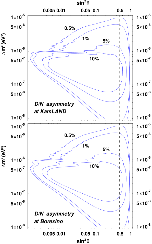
Figure 1: Constant day-night asymmetry contours ($10\%,5\%,1\%,0.5\%$) in the ($\sin^{2}\theta,\Delta m^{2}$)-plane for ⁷Be neutrinos at the KamLAND and Borexino sites. The vertical dashed line indicates $\sin^{2}\theta=1/2$, where the neutrino vacuum mixing is maximal.

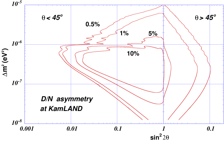
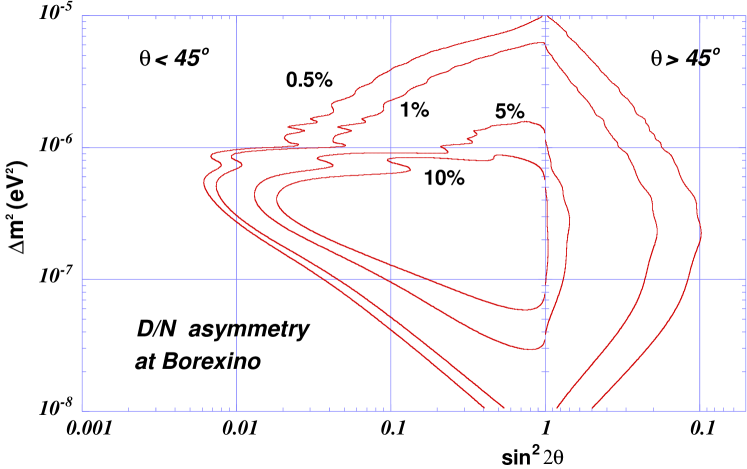
Figure 2: Constant day-night asymmetry contours ($10\%,5\%,1\%,0.5\%$) in the ($\sin^{2}2\theta,\Delta m^{2}$)-plane for ⁷Be neutrinos at the KamLAND and Borexino sites. The right side of the plot, with decreasing scale, can also be thought of as $\Delta m^{2}<0$, $\theta<45^{\rm 0}$.

Fig. 1 depicts the constant day-night asymmetry contours for ⁷Be neutrinos at KamLAND and Borexino. It is important to note that, unlike conventionally done in the literature, the $x$-axis here is $\sin^{2}\theta$, not $\sin^{2}2\theta$. To facilitate comparison with earlier results, we also depict the same information in the ($\Delta m^{2},\sin^{2}2\theta$) plane in Fig. 2, where once again we vary the mixing angle in its entire physical range $0\leq\theta\leq\pi/2$.

As Fig. 1 demonstrates, the asymmetry contours smoothly extend into the $\sin^{2}\theta>0.5$ half of the parameter space. One can see that in that region the day-night asymmetry is non-zero and may, in fact, be quite large. This kind of behavior had already been seen in [16], for day-night asymmetry contours at SuperKamiokande (see Fig. 11 in [16]). This is to be contrasted with conventional analyses, which choose axes as in Fig. 2, but only show the $0\leq\theta\leq\pi/4$ half of the parameter space. As a result, contours there seem to abruptly terminate at maximal mixing.

It is also easy to see from our plots that, with the choice of variables as in Fig. 1, there is nothing special about maximal mixing. This point is somewhat obscured in the ($\Delta m^{2},\sin^{2}2\theta$) plane, where it seems that the slope of the contours abruptly changes around $\sin^{2}2\theta=1$. The reason for this is that the Jacobian of the transformation from $\sin^{2}\theta$ to $\sin^{2}2\theta$,

$$\frac{d(\sin 2\theta)}{d(\sin\theta)}=2\frac{\cos 2\theta}{\cos\theta},$$ (2.5)

vanishes at maximal mixing $\theta=\pi/4$. It can be argued, therefore, that $\sin^{2}\theta$ represents a more natural parametrization. From here on we will always use $\sin^{2}\theta$ as a parameter.

The day-night asymmetry for $\theta=\pi/4$ is in general non-zero and, indeed, can be larger than 10%. Our analysis, thus, is in complete agreement with the findings of [17] and extends them to the other half of the parameter space. Note that constant day-night asymmetry contours do close as $\sin^{2}\theta\rightarrow 1$. This is expected, because in that limit, just like for $\sin^{2}\theta\rightarrow 0$, there is no neutrino mixing, and so $P_{ee}$ goes trivially to 1 and $A_{DN}$ vanishes.

Almost all other features of the contours in Figs. 1 and 2 can also be understood analytically. Several physical effects are involved in shaping up the contours. In the low $\Delta m^{2}$ region the oscillation length in the Earth is comparable to the size of the Earth, independent of the value of $\Delta m^{2}$. This can be understood very easily in the approximation that the Earth’s electron density is uniform. In that case the neutrino oscillation length is given by

$$L_{osc}=\pi\left[\left(\frac{\Delta m^{2}}{2E_{\nu}}\right)^{2}+(\sqrt{2}G_{F}N_{e})^{2}-2\left(\frac{\Delta m^{2}}{2E_{\nu}}\right)\sqrt{2}G_{F}N_{e}\cos 2\theta\right]^{-1/2},$$ (2.6)

or numerically

$$L_{osc} = 10.7\times 10^{4}\>{\rm km}\left[\left(\frac{\Delta m^{2}}{10^{-7}\>{\rm eV}^{2}}\right)^{2}+\left(1.3\frac{N_{e}}{1\>{\rm mole/cm^{3}}}\right)^{2}\right.$$ (2.7)

$$- \left.2\left(\frac{\Delta m^{2}}{10^{-7}\>{\rm eV}^{2}}\right)\left(1.3\frac{N_{e}}{1\>{\rm mole/cm^{3}}}\right)\cos 2\theta\right]^{-1/2},$$

and, for $\Delta m^{2}/(2E_{\nu})\ll\sqrt{2}G_{F}N_{e}$, $L_{osc}\rightarrow 8.2\cdot 10^{3}{\>\rm km}\times(1\>{\rm mole/cm^{3}}/N_{e})$.

For very small $\Delta m^{2}$ the asymmetry vanishes for two reasons. First, the MSW transition inside the Sun becomes non-adiabatic. For $\Delta m^{2}\ll 10^{-5}$ eV², $\theta_{M}\simeq\pi/2$ (Eq. (A.7)) in the Sun’s core and $P_{1}\simeq P_{c}$ (Eq. (A.9)). As the value of the jumping probability $P_{c}$ changes from 0 to $\cos^{2}\theta$ it passes through 1/2 (for $\theta<\pi/2$) where $A_{DN}$ vanishes, according to Eq. (2.4). As can be deduced from Eq. (A.18), the contours of constant jumping probability $P_{c}$ are approximately described by $\Delta m^{2}\sin^{2}\theta=$ constant, provided $\sin^{2}\theta\ll 1$ and $\Delta m^{2}\gg 10^{-9}$ eV². Second, the mixing angle in the Earth becomes close to $\pi/2$ and no regeneration takes place in that limit (see also Eq. (2.10) below, where $\theta_{M}\rightarrow\pi/2$ gives $P_{2e}^{av}\rightarrow\sin^{2}\theta$). Below the line $P_{1}=1/2$ the asymmetry is negative and very small.

In the region $\Delta m^{2}\mathrel{\mathchoice{\lower 3.0pt\vbox{\halign{$\m@th\displaystyle\hfill#\hfil$\cr>\crcr\sim\crcr}}}{\lower 3.0pt\vbox{\halign{$\m@th\textstyle\hfill#\hfil$\cr>\crcr\sim\crcr}}}{\lower 3.0pt\vbox{\halign{$\m@th\scriptstyle\hfill#\hfil$\cr>\crcr\sim\crcr}}}{\lower 3.0pt\vbox{\halign{$\m@th\scriptscriptstyle\hfill#\hfil$\cr>\crcr\sim\crcr}}}}3\times 10^{-6}$ eV² neutrinos undergo many oscillations inside the Earth, as can be seen from Eq. (2.7). The relevant quantity in this case is the average survival probability, obtained after integrating over the zenith angle. One can understand the shape of the asymmetry contours in this region by, once again, approximating the electron number density in the Earth by a constant value. In this model, it is easy to show that, if a state $|\nu_{i}\rangle$ enters from vacuum into the Earth, the average survival probability inside the Earth is

$$\begin{array}[]{cc}P_{2e}^{av}=\sin^{2}\theta_{M}+\sin^{2}(\theta-\theta_{M})\cos 2\theta_{M},&\;\;|\nu_{i}\rangle=|\nu_{2}\rangle,\\ P_{1e}^{av}=\sin^{2}\theta_{M}+\cos^{2}(\theta-\theta_{M})\cos 2\theta_{M},&\;\;|\nu_{i}\rangle=|\nu_{1}\rangle.\\ \end{array}$$ (2.10)

Here $\theta$ is the mixing angle in vacuum and $\theta_{M}$ is the mixing angle inside the Earth (see Eq. (A.7)). Obviously, $P_{1e}^{av}+P_{2e}^{av}=1$. Using these expressions, one can compute the day-night asymmetry for this simplified model:

$$A=\frac{P_{N}+(1-P_{N})R-P_{D}-(1-P_{D})R}{P_{N}+(1-P_{N})R+P_{D}+(1-P_{D})R},$$ (2.11)

where

$$P_{D} = \sin^{2}\theta_{\odot}((1-P_{c})\sin^{2}\theta+P_{c}\cos^{2}\theta)+$$

$$\cos^{2}\theta_{\odot}((1-P_{c})\cos^{2}\theta+P_{c}\sin^{2}\theta),$$

$$P_{N} = \sin^{2}\theta_{\odot}((1-P_{c})P_{2e}^{av}+P_{c}P_{1e}^{av})+$$

$$\cos^{2}\theta_{\odot}((1-P_{c})P_{1e}^{av}+P_{c}P_{2e}^{av}).$$

$\theta_{\odot}$ denotes the mixing angle at the production region in the core of the Sun, $P_{c}$ the jumping probability (Eq. (A.18)), and $R$ is a contribution of $\nu_{\mu,\tau}$ interacting through the neutral current interactions in the detector. We found that for $N_{e}\sim 3-4$ moles/cm³ the contours of constant $A$ are in good agreement with the day-night asymmetry contours in Fig. 1 for $\Delta m^{2}\mathrel{\mathchoice{\lower 3.0pt\vbox{\halign{$\m@th\displaystyle\hfill#\hfil$\cr>\crcr\sim\crcr}}}{\lower 3.0pt\vbox{\halign{$\m@th\textstyle\hfill#\hfil$\cr>\crcr\sim\crcr}}}{\lower 3.0pt\vbox{\halign{$\m@th\scriptstyle\hfill#\hfil$\cr>\crcr\sim\crcr}}}{\lower 3.0pt\vbox{\halign{$\m@th\scriptscriptstyle\hfill#\hfil$\cr>\crcr\sim\crcr}}}}3\times 10^{-6}$ eV².

Using this simple model we can explain the behavior of the asymmetry contours in the large $\Delta m^{2}$ region. For example, according to Fig. 1, as $\sin^{2}\theta$ decreases for fixed $\Delta m^{2}$, the value of the asymmetry goes down. This happens because, while the difference in the numerator of Eq. (2.11) goes to zero, the denominator approaches a constant value due to the non-vanishing neutral current contribution. Notice that in a real experiment, in addition to the neutral current contribution, there will be a term proportional to the rate of background events, further decreasing the sensitivity. Thus, using asymmetry contours in this region to read off the sensitivity can be misleading. This would be even more obvious in the case of oscillations to a sterile neutrino. We will return to this issue in the next section.

Even more subtle features can be understood within this model. For instance, we found that the slight change of the slope seen for the 0.5% contour around $\sin^{2}\theta\sim 0.04$ is due to the significant deviation of the value of $\theta_{\odot}$ from $\pi/2$ in that region.

Finally, in the region $\Delta m^{2}\sim 10^{-6}$ eV² the regeneration efficiency exhibits a very strong zenith angle dependence. Because the magnitudes of $\Delta m^{2}/(2E_{\nu})$ and $\sqrt{2}G_{F}N_{e}$ in the core are almost equal, the mixing in the core is almost maximal ($\theta_{M}\sim\pi/4$, see Eq. (A.7)), while in the mantle it is small ($\theta_{M}\sim\pi/2$). As a result, for neutrinos traveling through the outer core the conversion into $\nu_{e}$ is much more efficient than for ones going only through the mantle. The oscillations do not average out completely in this case, resulting in the presence of several wiggles. We have explicitly checked that these wiggles are not washed out by the effect of the finite width of the ⁷Be line [24].

Our results for $\theta<\pi/4$ agree qualitatively with the results presented in [15] for the Borexino site. The agreement is not complete, however. For instance, the contours in [15] do not exhibit any wiggles in the range $\Delta m^{2}\sim 10^{-6}$ eV².

3 The Neutrino Regeneration Effect at KamLAND and Borexino

In this section we study the sensitivity of the KamLAND and Borexino experiments to the day-night effect.

Borexino [25] is a dedicated ⁷Be solar neutrino experiment. It is a large sphere containing ultrapure organic liquid scintillator (300 t) and can detect the light emitted by recoil electrons produced by elastic $\nu$-$e$ scattering. By looking in the appropriate recoil electron kinetic energy window, it is possible to extract a very clean sample of events induced by ⁷Be neutrinos, if the number of background events is sufficiently small. Borexino expects, in the absence of neutrino oscillations, 53 neutrino induced events/day according to the SSM, and 19 events/day induced by background (mainly radioactive impurities in the detector, see [12, 25] for details).

The KamLAND experiment, located in the site of the original Kamiokande experiment, was initially designed as a reactor neutrino experiment. Recently, however, the fact that KamLAND might be used as a solar neutrino experiment has become a plausible and exciting possibility [26].

KamLAND is also a very large sphere containing ultrapure liquid scintillator (1 kt), and functions exactly like Borexino. The outstanding issue to determine if KamLAND will study solar neutrinos is if the background rates can be appropriately reduced. KamLAND expects, in the absence of neutrino oscillations, 466 neutrino induced events/kt/day according to the SSM, and 217 events/kt/day induced by background (mainly radioactive impurities in the detector, see [12, 26] for details). We will consider a fiducial volume of 600 t, so that 280 (unoscillated) signal events/day and 130 background events/day are expected. We assume that the number of background events is constant in time.

We generate a histogram of the number of events expected in each of the $N$ day and $N$ night bins for different values of ($\Delta m^{2},\sin^{2}\theta$). The number of events per year in the $i$-th bin is

$$n_{i}\left(\frac{\rm events}{\rm year}\right)=365\left(\frac{\rm days}{\rm year}\right)(b_{\rm rate}+s_{\rm rate}(P_{ee}^{i}+(1-P_{ee}^{i})R))\left(\frac{\rm events}{\rm day}\right)f_{i},$$ (3.1)

where $s_{\rm rate}=280$ (53) events/day and $b_{\rm rate}=130$ (19) events/day for KamLAND (Borexino), $P_{ee}^{i}$ is the electron neutrino survival probability in the $i$-th bin, $R$ is the ratio of the $\nu_{e}$-$e$ to $\nu_{\mu,\tau}$-$e$ elastic cross sections (see [12], at KamLAND (Borexino) $R=0.214$ (0.213)) and $f_{i}$=(size $i$-th bin divided by the sum of the sizes of all the bins), such that $\sum_{i}^{2N}f_{i}=1$. As an example, if there are 24 (12 day, 12 night) hour-bins, $f_{i}=1/24$ for all $i$. In reality, we are interested in zenith angle bins, and in order to the determine $f_{i}$, the exposure function presented in [15] is used. Note that we assume only statistical uncertainties.

$\chi^{2}$ is defined as

$$\chi^{2}=\sum_{i=1}^{N}\frac{\left(n_{i}^{\rm night}-n_{i}^{\rm day}\right)^{2}}{\left(\sqrt{n_{i}^{\rm night}}\right)^{2}+\left(\sqrt{n_{i}^{\rm day}}\right)^{2}}+N.$$ (3.2)

The factor $N$ is included in the definition of $\chi^{2}$ in order to take statistical fluctuations of the data into account. A detailed explanation of the philosophy behind this procedure can be found in [12].

It is important to comment at this point that, in light of the definition of $\chi^{2}$ (Eq. (3.2)), the sensitivity of the experiments to the Earth matter effect does not require any input from the SSM, including the ⁷Be solar neutrino flux, or from a direct measurement of the background rate. This is because we are comparing the night data with the day data, and no other inputs are required. Our quantitative results, however, depend on the expected number of signal and background induced events, since these quantities are used as input for the “data” sample.

We will define the sensitivity of a given experiment to the Earth matter effect by the value of $\chi^{2}$, computed according to Eq. (3.2). The sensitivity defined in this way depends clearly on $N$, the number of day and night bins, and on $f_{i}$ (see Eq. (3.1)), or on the “size of the bin”. With the real experimental data, one will certainly consider many different types of analyses in order to maximize the sensitivity of the data to the neutrino regeneration in the Earth (options include computing moments of the zenith angle distribution, Fourier decomposing the data, maximum likelihood analysis, and others), but, since we analyze thousands of “data samples” (one for each value of ($\Delta m^{2},\sin^{2}\theta$)), this simple $\chi^{2}$ approach will suffice.

We consider two options for the size of zenith angle bins. In one of them, each bin has the same size, that is, the bins are equally spaced (e.g. $0^{\rm o}-30^{\rm o},30^{\rm o}-60^{\rm o},60^{\rm o}-90^{\rm o}$, etc). The other option is to choose the bin size such that the distribution of the day data is uniform. It is worthwhile to comment that the latter scheme may be considered the most natural one for KamLAND and Borexino, which are real time experiments with no directional capability. In these experiments, it is straightforward to organize the data into time bins, which then have to be translated into zenith angle bins by associating the time of the event with the position of the Sun in the sky.

Another issue to consider is the value of $N$ which optimizes the sensitivity. It is clear that for $N=1$ (the day-night asymmetry case) the statistical significance is enhanced for overall changes in the number of events, but for larger $N$, one should be more sensitive to distortions in the zenith angle distribution. Different binning schemes of the “data” for $\Delta m^{2}=1.12\times 10^{-7}$ eV², $\sin^{2}\theta=0.398$ and three years of KamLAND running are depicted in Fig. 3, for $N=1$, $N=10$ equally spaced bins, and $N=10$ “uniform” bins.

Figure 3: Different binning schemes, for $\Delta m^{2}=1.12\times 10^{-7}$ eV², $\sin^{2}\theta=0.398$: (a) $N=1$ bin (the day-night asymmetry), (b) $N=10$ equally spaced zenith angle bins, and (c) $N=10$ “uniform” bins, where the day-time data is (roughly) uniformly distributed. The error bars contain statistical uncertainties only. We assume three years of KamLAND running.

Fig. 4 shows a comparison of the sensitivity reach of KamLAND after three years of running for two different binning schemes, $N=1$ vs. $N=10$ “uniform” bins. The contours are drawn at 95% C.L. One can easily see that for most of the parameter space, the best sensitivity is reached with the $N=1$ case, while for a small region in the parameter space, when $\sin^{2}\theta\mathrel{\mathchoice{\lower 3.0pt\vbox{\halign{$\m@th\displaystyle\hfill#\hfil$\cr<\crcr\sim\crcr}}}{\lower 3.0pt\vbox{\halign{$\m@th\textstyle\hfill#\hfil$\cr<\crcr\sim\crcr}}}{\lower 3.0pt\vbox{\halign{$\m@th\scriptstyle\hfill#\hfil$\cr<\crcr\sim\crcr}}}{\lower 3.0pt\vbox{\halign{$\m@th\scriptscriptstyle\hfill#\hfil$\cr<\crcr\sim\crcr}}}}0.1$ and $\Delta m^{2}\sim 10^{-6}$ eV², the $N=10$ scheme is more successful. This result is consistent with the analysis of Section 2.2. As explained there, for $\Delta m^{2}\sim 10^{-6}$ eV² the data shows a large enhancement in the low zenith angle bin, while little effect in other bins. At Borexino this effect will be somewhat less pronounced because it is farther from the Equator.

One can see that the contours in Fig. 4 are similar in shape to the day-night asymmetry contours of Section 2.2, but quantitatively different. One important difference is that for $\Delta m^{2}\mathrel{\mathchoice{\lower 3.0pt\vbox{\halign{$\m@th\displaystyle\hfill#\hfil$\cr>\crcr\sim\crcr}}}{\lower 3.0pt\vbox{\halign{$\m@th\textstyle\hfill#\hfil$\cr>\crcr\sim\crcr}}}{\lower 3.0pt\vbox{\halign{$\m@th\scriptstyle\hfill#\hfil$\cr>\crcr\sim\crcr}}}{\lower 3.0pt\vbox{\halign{$\m@th\scriptscriptstyle\hfill#\hfil$\cr>\crcr\sim\crcr}}}}10^{-6}$ eV² the $\chi^{2}$ contours do not extend as far in the low $\sin^{2}\theta$ region as the asymmetry contours. While for low $\Delta m^{2}$ the 95% C.L. contour corresponds to the day-night asymmetry of roughly 0.5%, for $\Delta m^{2}\mathrel{\mathchoice{\lower 3.0pt\vbox{\halign{$\m@th\displaystyle\hfill#\hfil$\cr>\crcr\sim\crcr}}}{\lower 3.0pt\vbox{\halign{$\m@th\textstyle\hfill#\hfil$\cr>\crcr\sim\crcr}}}{\lower 3.0pt\vbox{\halign{$\m@th\scriptstyle\hfill#\hfil$\cr>\crcr\sim\crcr}}}{\lower 3.0pt\vbox{\halign{$\m@th\scriptscriptstyle\hfill#\hfil$\cr>\crcr\sim\crcr}}}}10^{-6}$ eV² the corresponding value of the day-night asymmetry is at least two times greater. This phenomenon was already mentioned in Section 2.2. The difference occurs because the $\chi^{2}$ analysis includes, in addition to the neutral current interactions, the constant background rate, thus eliminating the major shortcoming of the day-night asymmetry analysis.

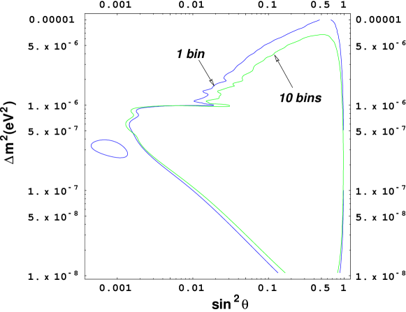
Figure 4: Comparison of the sensitivity reach of three years of KamLAND running with 1 bin and 10 uniform bins.

In order to present the final sensitivity reach of KamLAND and Borexino, we combine the confidence level contour obtained in the different types of analyses, with different number of bins. Fig. 5 depicts the “optimal” 95%, 3$\sigma$, and 5$\sigma$ confidence level (C.L.) contours for the sensitivity of three years of KamLAND and Borexino data to the day-night effect. The confidence levels are optimized by considering the union of same C.L. contours for all values of $N$ and both binning schemes. The day-night asymmetry provides the best sensitivity reach for most of the parameter space, while the $N\approx 10$ uniform bins scheme at KamLAND increases the sensitivity for particular regions of the parameter space, as was discussed earlier.

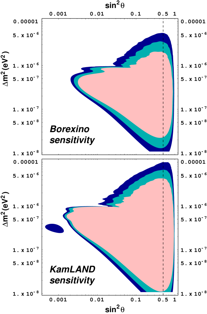
Figure 5: 95% (darkest), 3$\sigma$ (dark), and 5$\sigma$ (light) sensitivity confidence level (C.L.) contours for three years of KamLAND running. The LOW solution, which extends from $\Delta m^{2}\sim 3\times 10^{-8}$ eV² to $\Delta m^{2}\sim 3\times 10^{-7}$ eV² and has $\sin^{2}\theta\sim 0.3-0.5$ [8], is completely covered at more than $5\sigma$ C.L.

Fig. 5 clearly demonstrates that in the case of the LOW MSW solution to the solar neutrino puzzle, both KamLAND and Borexino should be able to see a larger than 5$\sigma$ effect, while in the case of the SMA no significant effect should be detected. Both experiments are sensitive to a large portion of the parameter space which extends into $\theta>\pi/4$ region, where the heavy neutrino eigenstate is predominantly $\nu_{e}$.

On the other hand, should no regeneration effect be observed, a large portion of the parameter space, including the entire LOW region might be excluded. The exclusion will require knowledge of the ⁷Be neutrino flux, which can be measured, for example, by studying the seasonal variation of the observed event rate [12]. If the flux measured in this way turns out large and no day-night asymmetry is observed, one will be able to exclude the LOW solution without relying on the solar model. If, however, the measured flux is very small, the exclusion will be solar model dependent.

Since the sensitivity of Borexino (KamLAND) to the day-night asymmetry goes down to the 1.5% (0.5%) level, it is important to consider systematic effects in this measurement. It is, however, difficult to anticipate systematic uncertainties in the absence of data. We instead looked at the measurement of day-night asymmetry at SuperKamiokande [18]. The dominant systematic uncertainty there is the possible asymmetry in the detector, giving $\pm 0.6\%$. Because the recoil electrons from ⁸B neutrinos are forward peaked, the day (night) time data are detected primarily by the lower (upper) half the detector. A small possible gain asymmetry ([18] quotes 0.5%) for different zenith angle bins can result is a somewhat amplified difference in rates because the energy spectrum is rather steep close to the threshold energy (6.5 MeV). The energy calibration was done using electron LINAC, which at that time could shoot electrons only downwards and hence could not study the asymmetry well enough. The gain asymmetry is known to exist from the study of decay electrons in the cosmic ray muon data [27] as well as in spallation events [28]. We assume that this will not be an important systematic effect for Borexino or KamLAND because the energy deposit is basically isotropic (no directional capability) and hence the asymmetry in the detector should not result in a systematic effect in the day-night asymmetry.

The next largest systematic effect is the subtraction of background, $\pm 0.2\%$. If the background events are not completely isotropic, the subtraction depends on the direction and results in a systematic effect. Again at Borexino or KamLAND, the lack of directional correlation eliminates this systematic effect.

If we naively drop these two dominant systematic effects, the size of the total systematic uncertainty would be less than 0.1%. Of course, the sources of background are very different at Borexino or KamLAND. Possible differences in the temperature or Rn level between the day and night times could introduce new systematic effects, while our analysis assumed the same background level for day and night. This difference, however, can in principle be measured using the Bi-Po coincidence. Spallation background (such as ¹¹C) should not change between day and night.

Additionally, the experiments will need to consider other effects, such as the contribution of other neutrino sources or the uncertainty in the electron number density profile of the Earth. (More on the latter in the next section.) We also did not include in our analysis the contribution of neutrinos produced in the CNO cycle, which is about 10% of that from the ⁷Be neutrinos. Although we cannot accurately predict the total systematic uncertainty at Borexino or KamLAND, we nonetheless find it encouraging that the dominant uncertainties at SuperKamiokande are unlikely to affect these experiments.

4 Measuring the Oscillation Parameters

In this section, we discuss the possibility of measuring the value of $\Delta m^{2},\sin^{2}\theta$ in the advent of a large day-night effect. In order to do this, data was simulated for $\Delta m^{2}=1.12\times 10^{-7}$ eV², $\sin^{2}\theta=0.398$, which is close to the LOW MSW solution to the solar neutrino puzzle [8]. For a plot of the “data” with different binning options, see Fig. 3.

In order to deal with the SSM solar neutrino flux and the background event rate, we will conservatively “measure” both the background rate and the incoming solar neutrino flux by analyzing the seasonal variation [12] of the day-time data only. This measurement procedure will be incorporated in a four parameter $\chi^{2}$ analysis (the parameters are $\Delta m^{2}$, $\sin^{2}\theta$, the solar neutrino flux $s$, and the background rate $b$) of the data. Explicitly,

$$\chi^{2}(\Delta m^{2},\sin^{2}\theta,s,b)=\sum^{N}_{i=1}\frac{\left({\rm data}_{i}^{\rm night}-{\rm theo}_{i}^{\rm dn}\right)^{2}}{\left(\sqrt{{\rm data}_{i}^{\rm night}}\right)^{2}}+\sum^{M}_{j=1}\frac{\left({\rm data}_{j}^{\rm day}-{\rm theo}_{j}^{\rm sea}\right)^{2}}{\left(\sqrt{{\rm data}_{j}^{\rm day}}\right)^{2}},$$ (4.1)

where data${}_{i}^{\rm night}$ is the night-time “data” binned into $N$ night bins (as described in Sec. 3), data${}_{j}^{\rm day}$ is the day-time “data” binned into $M$ “seasonal bins” (e.g. $j=1,2,\dots 12$ months) as described in [12]. theo${}_{i}^{\rm dn}$ is the prediction for the number of evens in the $i$-th night bin,

$${\rm theo}_{i}^{\rm dn}=365\left[b+s(P_{ee,i}^{\rm night}+(1-P_{ee,i}^{\rm night})R)\right]f_{i},$$ (4.2)

similar to Eq. (3.1). $b$ is the background rate in events per day and $s$ is the number of events per day induced solar neutrinos according to the SSM prediction for the solar neutrino flux. Similarly, theo${}_{j}^{\rm sea}$ is the prediction for the day-time flux in the $j$-th seasonal bin (see [12]),

$${\rm theo}_{j}^{\rm sea}=\left[\int_{i-1}^{i}{\rm d}t\left(b+s\frac{P_{ee}+(1-P_{ee})R}{(1-\epsilon\cos(2\pi t/{\rm year}))^{2}}\right)\right]g_{j},$$ (4.3)

where $g_{j}$ is the number of days in the $j$-th bin and $\epsilon=0.017$ is the eccentricity of the Earth’s orbit.

It is simple to minimize $\chi^{2}$ with respect to $s$ and $b$, given that $\chi^{2}(s,b)$ is a quadratic function. The minimization with respect to $\Delta m^{2}$ and $\sin^{2}\theta$ is done numerically. Fig. 6 depicts the extracted contours in the ($\Delta m^{2},\sin^{2}\theta$)-plane, in the case of 1 night bin and 10 “uniform” night bins, respectively.

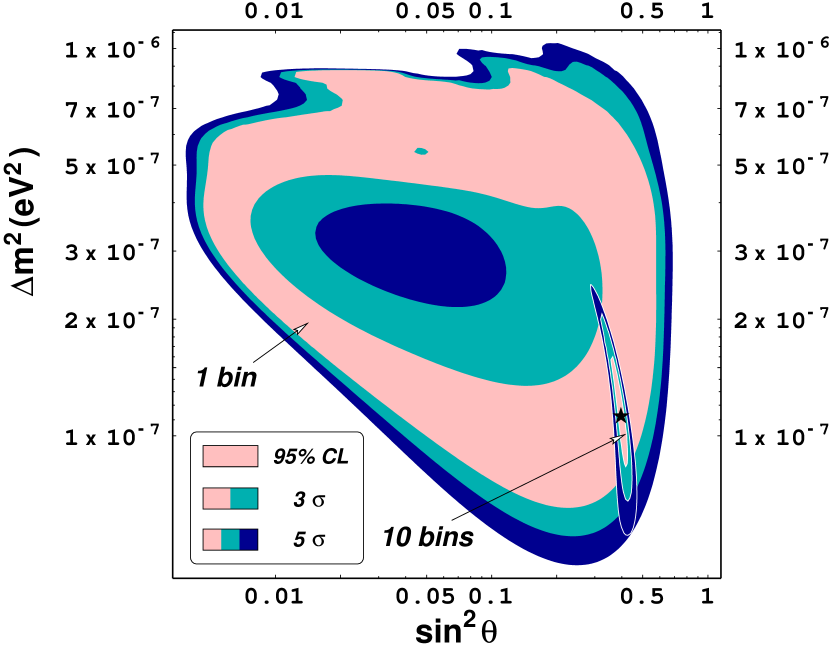
Figure 6: Measured values of ($\Delta m^{2},\sin^{2}\theta$) at KamLAND after three years of running. The data was generated for $\Delta m^{2}=1.12\times 10^{-7}$ eV², $\sin^{2}\theta=0.398$ (marked with the “star”). The regions obtained by using one night bin and ten uniform night bins are shown.

As Fig. 6 demonstrates, in the case of 1 night bin, one extracts values of $\Delta m^{2}$ and $\sin^{2}\theta$ which fall into “rings” which correspond roughly to $A_{DN}=A_{DN}^{\rm real}\pm\Delta A_{DN}^{\rm real}$, where $A_{DN}^{\rm real}$ is the value of the day-night asymmetry for the input value of $\Delta m^{2},\sin^{2}\theta$. In the case of more than one uniform bin, the ring degeneracy is broken, and a much more precise determination of the oscillation parameters is possible. This is expected, since for $\Delta m^{2}$ in this range the regeneration effect in the Earth exhibits a strong zenith angle dependence, as one can easily verified by looking at Fig. 3.

It is important to note that in the above analysis only statistical uncertainties were included, while in a real experiment one definitely will have to account for systematic effects as well. In particular, one will need to address the uncertainty in the Earth model used in the fit. In producing Fig. 6 the same Earth model [23] was used in generating the “data” and in the fit procedure. To understand the effect of using a “wrong” Earth model, we have repeated the above analysis using different Earth models in the fit. We found the results very encouraging. Even in the case when we used for the Earth profile a crude two-step model (a uniform density in the mantle and a uniform density in the core), the minimum of $\chi^{2}$ occurred at $\Delta m^{2}=2.5\times 10^{-7}$ eV², $\sin^{2}\theta=0.24$, not far away from the true (input) value. Moreover, the $\chi^{2}$ value at the minimum was much larger than the case with the “true” model ($\Delta\chi^{2}=183$ for 18 d.o.f.). This means that in a real experiment one will be able to adjust the Earth’s model to achieve a better fit to the data. Because of the steep rise in $\chi^{2}$ value as the Earth model is varied, the resulting $\chi^{2}$ contours in the $(\Delta m^{2},\sin^{2}\theta)$ parameter space should not be significantly larger than the ones presented here, where the Earth model is not varied. As a byproduct of the measurement of the neutrino oscillation parameters, it might be possible to use the regeneration data to study the interior of the Earth!

5 Conclusions

We have studied the effect of the Earth matter on ⁷Be solar neutrinos. We made use of an enlarged parameter space $0\leq\theta\leq\pi/2$ and presented the sensitivity reach of the KamLAND and Borexino experiments in this space. Our results show that both experiments will be sensitive to the Earth regeneration effect in a large region which extends into the traditionally neglected $\theta>\pi/4$ part of the parameter space. In particular, for the LOW solution one expects to see a greater than $5\sigma$ effect. On the other hand, both experiments will see no day-night effect for the SMA solution and virtually no effect for the LMA solution.

If the experiments see a large Earth regeneration effect, it will be a powerful “smoking gun” signature of neutrino oscillations. Furthermore, as we have demonstrated, the results of the experiments can be used to measure the oscillation parameters. By studying the full zenith angle distribution, rather than the usual day-night asymmetry information, one might be able, in the case of the LOW solution, to perform a spectacular measurement of the parameters. In addition, it might be possible to use the zenith angle information to learn about the Earth electron density profile.

If, on the other hand, no Earth regeneration effect is detected, by combining this information with the flux measurement from seasonal variation of the event rate [12], a large portion of the parameter space can be excluded. If the measured value of the ⁷Be neutrino flux is large, the exclusion will be independent of a specific solar model.

Both the measurement of the oscillation parameters and the exclusion will require a thorough understanding of the systematic uncertainties. We have commented on some possible sources of such uncertainties in this paper.

Overall, Borexino and KamLAND will provide crucial information about the solar neutrinos. Not only will the experiments measure the flux of the ⁷Be solar neutrinos, but they will also be able to establish or exclude, without relying on solar models, the LOW solution based on the Earth regeneration effect and the vacuum oscillation solution based on the observed seasonal variation of the event rate. Together with results from SuperKamiokande, SNO, and the KamLAND reactor neutrino experiment, this information can be used to finally unravel the 30-year-old solar neutrino puzzle.

Appendix A Matter Oscillations and No Level Crossing

In this appendix, we discuss the survival probability of solar electron neutrinos outside the Sun, in particular the case of no level crossing, i.e., when $\Delta m^{2}\cos 2\theta<0$ in the language of the two neutrino mixing scenario.

In the literature, matter effects in the Sun are always considered when there is “level crossing” inside of the Sun, i.e., when the light neutrino is predominantly of the electron type, and, due to neutrino-electron interactions, when the instantaneous Hamiltonian eigenstate with the largest eigenvalue is predominantly of the electron type in the Sun’s core. The other case, when the heavy neutrino is predominantly of the electron type, has not been studied in the literature in the context of two neutrino oscillations. The authors of [16], however, have considered this possibility in the context of three-flavor oscillations.

The reason for this apparent neglect is simple, and will become clear as our results are presented. What happens is that, in the case of no level crossing, the electron neutrino survival probability is always bigger than 1/2, and therefore it seems that this scenario is not relevant to the solar neutrino puzzle. This, however, may not be the case [30].

Before presenting the expressions for the electron neutrino survival probability outside of the Sun, it is necessary to clearly define the neutrino eigenstates and mixing angles. The neutrino mass eigenstates are defined in Eq. (2.1), and the notation introduced in Sec. 2 will be used. In what follows our convention is $\Delta m^{2}>0$ and $0\leq\sin^{2}\theta\leq 1$.

Inside the Sun the Hamiltonian has the form

$$H=p_{\nu}+\frac{m^{2}_{\rm sum}}{4p_{\nu}}-\sqrt{2}G_{F}N_{n}(r)/2$$ (A.3)

$$+\left(\begin{array}[]{cc}-\frac{\Delta m^{2}}{4p_{\nu}}\cos 2\theta+\sqrt{2}G_{F}N_{e}(r)&\frac{\Delta m^{2}}{4p_{\nu}}\sin 2\theta\\ \frac{\Delta m^{2}}{4p_{\nu}}\sin 2\theta&\frac{\Delta m^{2}}{4p_{\nu}}\cos 2\theta\\ \end{array}\right),$$

were $p_{\nu}$ is the solar neutrino momentum, $N_{e}(r)$ ($N_{n}(r)$) is the electron (neutron) number density at a distance $r$ from the Sun’s core, $m^{2}_{\rm sum}\equiv m_{2}^{2}+m_{1}^{2}$ and $\Delta m^{2}\equiv m_{2}^{2}-m_{1}^{2}$, $m_{2}^{2}$ and $m_{1}^{2}$ being the mass eigenvalues in vacuum. The eigenvalues of the instantaneous Hamiltonian are

$$\lambda_{\pm}(r) = p_{\nu}+\frac{m_{\rm sum}^{2}}{4p_{\nu}}+\frac{\sqrt{2}G_{F}(N_{e}(r)-N_{n}(r))}{2}\pm\frac{1}{2}\left[\left(\frac{\Delta m^{2}}{2p_{\nu}}\right)^{2}\right.$$ (A.4)

$$+ \left.\left(\sqrt{2}G_{F}N_{e}(r)\right)^{2}-\frac{\Delta m^{2}}{p_{\nu}}\sqrt{2}G_{F}N_{e}(r)\cos 2\theta\right]^{1/2}.$$

For the study of neutrino oscillations, terms common to both states are irrelevant, and the first three terms can be dropped. One can also safely replace $p_{\nu}$ by $E_{\nu}$ in the remainder. The instantaneous Hamiltonian eigenstates in terms of flavor eigenstates are

$$|\nu_{-}(r)\rangle=\cos\theta_{M}(r)|\nu_{e}\rangle-\sin\theta_{M}(r)|\nu_{\mu}\rangle,$$ (A.5)

$$|\nu_{+}(r)\rangle=\sin\theta_{M}(r)|\nu_{e}\rangle+\cos\theta_{M}(r)|\nu_{\mu}\rangle.$$ (A.6)

Here $\theta_{M}(r)$ is the matter mixing angle, given by

$$\cos 2\theta_{M}(r)=$$ (A.7)

$$\frac{\Delta m^{2}\cos 2\theta-2E_{\nu}\sqrt{2}G_{F}N_{e}(r)}{\sqrt{(\Delta m^{2})^{2}+(2E_{\nu}\sqrt{2}G_{F}N_{e}(r))^{2}-4\Delta m^{2}E_{\nu}\sqrt{2}G_{F}N_{e}(r)\cos 2\theta}}.$$

Assuming that $N_{e}\rightarrow 0$ as $r\rightarrow\infty$, it is easy to see that $|\nu_{+}(r\rightarrow\infty)\rangle\rightarrow|\nu_{2}\rangle$ and $|\nu_{-}(r\rightarrow\infty)\rangle\rightarrow|\nu_{1}\rangle$. Therefore, if the transition from the core of the Sun to vacuum is adiabatic, a state which is created as a $|\nu_{+}(0)\rangle$ ($|\nu_{-}(0)\rangle$) will exit the Sun as a $|\nu_{2}\rangle$ ($|\nu_{1}\rangle$).

Having established the notation, it is very easy to estimate the survival probability for electron neutrinos that are created in the Sun’s core and are detected on the Earth, in the limit that $\Delta m^{2}/2E_{\nu}$ is much smaller than the Earth-Sun distance, such that oscillations in vacuum between $\nu_{1}$ and $\nu_{2}$ states are “averaged out.” There are four possible “propagation paths” that the solar neutrino can follow:

$$\nu_{e} \rightarrow \nu^{+}(p=\sin^{2}\theta_{M})\rightarrow\nu_{2}(p=1-P_{c})\rightarrow\nu_{e}(p=\sin^{2}\theta)$$

or

$$\nu_{e} \rightarrow \nu^{+}(p=\sin^{2}\theta_{M})\rightarrow\nu_{1}(p=P_{c})\rightarrow\nu_{e}(p=\cos^{2}\theta)$$ (A.8)

or

$$\nu_{e} \rightarrow \nu^{-}(p=\cos^{2}\theta_{M})\rightarrow\nu_{1}(p=1-P_{c})\rightarrow\nu_{e}(p=\cos^{2}\theta)$$

or

$$\nu_{e} \rightarrow \nu^{-}(p=\cos^{2}\theta_{M})\rightarrow\nu_{2}(p=P_{c})\rightarrow\nu_{e}(p=\sin^{2}\theta),$$

where $p$ is the probability that a given “step” takes place, $\theta_{M}=\theta_{M}(0)$ and $P_{c}$ is the jumping probability, i.e. the probability that during the evolution from the Sun’s core to vacuum the neutrino changes from one set of instantaneous Hamiltonian eigenstates to the other.

Therefore, the probabilities of finding the mass eigenstates $\nu_{1}$ and $\nu_{2}$ far from the Sun are given by

$$P_{1} = \sin^{2}\theta_{M}P_{c}+\cos^{2}\theta_{M}(1-P_{c})$$ (A.9)

$$P_{2} = 1-P_{1},$$ (A.10)

where $\theta_{M}$ is that at the production point, and the electron neutrino survival probability ($P_{ee}$) at the surface of the Earth is

$$P_{ee} = P_{1}\cos^{2}\theta+P_{2}\sin^{2}\theta$$ (A.11)

$$= \sin^{2}\theta_{M}((1-P_{c})\sin^{2}\theta+P_{c}\cos^{2}\theta)$$

$$+ \cos^{2}\theta_{M}((1-P_{c})\cos^{2}\theta+P_{c}\sin^{2}\theta).$$

All equalities hold as long as two mass eigenstates appear as an incoherent mixture (true for $\Delta m^{2}\mathrel{\mathchoice{\lower 3.0pt\vbox{\halign{$\m@th\displaystyle\hfill#\hfil$\cr>\crcr\sim\crcr}}}{\lower 3.0pt\vbox{\halign{$\m@th\textstyle\hfill#\hfil$\cr>\crcr\sim\crcr}}}{\lower 3.0pt\vbox{\halign{$\m@th\scriptstyle\hfill#\hfil$\cr>\crcr\sim\crcr}}}{\lower 3.0pt\vbox{\halign{$\m@th\scriptscriptstyle\hfill#\hfil$\cr>\crcr\sim\crcr}}}}10^{-8}$ eV² for ⁷Be neutrinos). In deriving Eq. (A.11), no assumption was made with respect to the value of $\cos 2\theta$, and therefore it should be valid for the entire range of $0\leq\sin^{2}\theta\leq 1$.

Given Eq. (A.11), it is easy to show that for $\theta<\pi/4$, $P_{ee}$ can be (much) smaller than 1/2, while for $\theta>\pi/4$, $P_{ee}$ is larger than 1/2 (indeed, it will be shown that $P_{ee}\geq P_{ee}^{v}$, the (averaged) vacuum survival probability).

First, note that $-1\leq\cos 2\theta_{M}\leq\cos 2\theta$. The equalities are saturated when $\sqrt{2}G_{F}N_{e}(0)\gg\Delta m^{2}/2E_{\nu}$ or $\sqrt{2}G_{F}N_{e}(0)\ll\Delta m^{2}/2E_{\nu}$, respectively. More quantitatively

$$\frac{\Delta m^{2}}{2E_{\nu}\sqrt{2}G_{F}N_{e}(0)}=0.98\left(\frac{\Delta m^{2}}{10^{-5}\rm eV^{2}}\right)\left(\frac{0.862\rm MeV}{E_{\nu}}\right),$$ (A.12)

for an average core electron number density of 79 moles/cm³ [10]. Therefore, in the case of ⁷Be neutrinos and $\Delta m^{2}\ll 10^{-5}$ eV²,

$$\cos 2\theta_{M}=-1+\frac{1}{2}\left(\frac{\Delta m^{2}\sin 2\theta}{2E_{\nu}\sqrt{2}G_{F}N_{e}(0)}\right)^{2}+{\cal O}\left(\frac{\Delta m^{2}}{2E_{\nu}\sqrt{2}G_{F}N_{e}(0)}\right)^{3},$$ (A.13)

and

$$P_{ee}\simeq(1-P_{c})\sin^{2}\theta+P_{c}\cos^{2}\theta.$$ (A.14)

We will soon show that $P_{c}\in[0,\cos^{2}\theta]$, so that, in the limit $\cos 2\theta_{M}\rightarrow-1$,

$$P_{ee}\in[\sin^{2}\theta,\sin^{4}\theta+\cos^{4}\theta] {\rm or}$$ (A.15)

$$P_{ee}\in[\sin^{4}\theta+\cos^{4}\theta,\sin^{2}\theta]$$ (A.16)

Eq. (A.15) (Eq. (A.16)) applies if $\sin^{2}\theta<\cos^{2}\theta$ ($\sin^{2}\theta>\cos^{2}\theta$). This is easy to see because $\sin^{4}\theta+\cos^{4}\theta=1-(1/2)\sin^{2}2\theta$ is the vacuum survival probability $P_{ee}^{v}$ and

$$P_{ee}^{v} = 1-2\sin^{2}\theta(1-\sin^{2}\theta)$$ (A.17)

$$= 1-2\sin^{2}\theta+2\sin^{4}\theta,$$

which is bigger (smaller) than $\sin^{2}\theta$ if $\sin^{2}\theta<\cos^{2}\theta$ ($\sin^{2}\theta>\cos^{2}\theta$).

When $\sqrt{2}G_{F}N_{e}(0)\ll\Delta m^{2}/2E_{\nu}$ matter interactions should be irrelevant, and it is easy to see from Eq. (A.7) that $\cos 2\theta_{M}\rightarrow\cos 2\theta$. In this limit $P_{c}\rightarrow 0$, since we are deep into the adiabatic region (as will be shown later) and $P_{ee}\rightarrow P_{ee}^{v}$. Before summarizing the behavior of the ⁷Be electron neutrino survival probability we will determine some expression for $P_{c}$.

Assuming an exponential profile for the electron number density inside the Sun ($N_{e}(r)=N_{e}(0)\exp(-r/r_{0})$), Schrödinger’s equation can be solved analytically [31, 21], and it is shown that, in the range of the neutrino oscillation parameter space relevant for addressing the solar neutrino puzzle, Eq. (A.11) is indeed a very good approximation for $P_{ee}$ and that $P_{c}$ is given by [21, 32]

$$P_{c}=\frac{e^{-\gamma\sin^{2}\theta}-e^{-\gamma}}{1-e^{-\gamma}},$$ (A.18)

where

$$\gamma=2\pi r_{0}\frac{\Delta m^{2}}{2E_{\nu}}=1.22\left(\frac{\Delta m^{2}}{10^{-9}\mbox{ eV}^{2}}\right)\left(\frac{0.862\mbox{ MeV}}{E_{\nu}}\right),$$ (A.19)

for $r_{0}=R_{\odot}/10.54=6.60\times 10^{4}$ km.

According to the author of [21], Eq. (A.18) only holds for $\Delta m^{2}\cos 2\theta>0$. We will prove shortly, however, that Eq. (A.18) also applies in the case of no level crossing, when the heavy mass eigenstate is predominantly of the electron type, i.e. when $\sin^{2}\theta>\cos^{2}\theta$. Assuming that this is indeed the case, we can finish our discussion on the behavior of the electron neutrino survival probability, using ⁷Be neutrinos as an example.

When $\Delta m^{2}\ll 10^{-9}$ eV², $\cos 2\theta_{M}=-1$ and $P_{c}=\cos^{2}\theta$. In this case we argued and one can explicitly check that $P_{ee}=P_{ee}^{v}$. For $10^{-9}$ eV${}^{2}\ll\Delta m^{2}\ll 10^{-5}$ eV², $\cos 2\theta_{M}=-1$ and $P_{c}\rightarrow 0$. In this case $P_{ee}\simeq\sin^{2}\theta$. This is the adiabatic region. For $\Delta m^{2}\gg 10^{-5}$ eV², matter effects become irrelevant and $\cos 2\theta_{M}=\cos 2\theta$, $P_{c}=0$. Again $P_{ee}=P_{ee}^{v}$. Therefore, Eqs. (A.15,A.16) apply for all values of interest, and one can get a very large suppression of $P_{ee}$ if $\sin^{2}\theta\ll 1$. On the other hand, in the case of no level crossing, $P_{ee}$ is always bigger than $P_{ee}^{v}\geq 1/2$.

Fig. 7 depicts the behavior of $P_{ee}^{(^{7}\rm Be)}$ as a function of $\Delta m^{2}$, for different values of the vacuum mixing angle. The preferred values from the overall rate analysis at the Homestake, Sage and Gallex, and SuperKamiokande experiments [8] are indicated by stars. The four plots are labeled SMA, LMA, LOW to indicate that they contain the best fit values of $\theta$ for the Small Mixing Angle, Large Mixing Angle and LOW $\Delta m^{2}$ solutions [8], respectively, and INT to indicate an intermediate value of $\theta$ between the SMA and LMA solutions. The dotted line indicates the value of $P_{ee}^{v}$. Similarly, Fig. 8 depicts $P_{ee}^{(^{7}\rm Be)}$ as a function of $\sin^{2}\theta$ for different values of the mass squared difference. We use the same notation as the one used in Fig. 7, and the vertical dashed lines indicate the mixing angle for maximal vacuum mixing ($\sin^{2}\theta=1/2$). Note that at this point $P_{ee}^{(^{7}\rm Be)}=P_{ee}^{v}=1/2$.

Figure 7: The electron neutrino survival probability as a function $\Delta m^{2}$, for different values of the vacuum mixing angle, namely, $\cos 2\theta=\pm 0.997$ (SMA), $\cos 2\theta=\pm 0.8$ (INT), $\cos 2\theta=\pm 0.58$ (LMA), and $\cos 2\theta=\pm 0.24$ (LOW). The upper (lower) lines are for the negative (positive) sign of $\cos 2\theta<0$. The stars indicate the preferred points from the overall rate analysis of the existing data [8], and the horizontal dotted lines indicate the vacuum survival probability, $P_{ee}^{v}=1/2-1/2\sin^{2}2\theta$ .

Figure 8: The electron neutrino survival probability as a function $\sin^{2}\theta$, for different values of $\Delta m^{2}$, namely, $\Delta m^{2}=1.3\times 10^{-7}$ eV² (LOW), $\Delta m^{2}=5.0\times 10^{-6}$ eV² (SMA), $\Delta m^{2}=1.4\times 10^{-5}$ eV²(LMA), and $\Delta m^{2}=1\times 10^{-4}$ eV². The stars indicate the preferred points from the overall rate analysis of the existing data [8], and the dashed lines indicate the vacuum survival probability, $P_{ee}^{v}=1/2-1/2\sin^{2}2\theta$.

Finally, we argue that Eq. (A.18) holds for all values of $\cos 2\theta$. When $\sqrt{2}G_{F}N_{e}(0)\gg|\Delta m^{2}|/2E_{\nu}$, it is very simple to derive $P_{ee}$, following the exact solution [31, 21] to Schrödinger’s equation and taking the appropriate limits. According to Eq. (39) in [21]

$$P_{\mu e} = \frac{\sin^{2}(2\theta)}{4}\left[\frac{\sinh(\pi r_{0}h_{0}\cos^{2}\theta)}{\cos^{2}\theta\sinh(\pi r_{0}h_{0})}e^{-\pi r_{0}h_{0}\sin^{2}\theta}\right.$$ (A.20)

$$+ \left.\frac{\sinh(\pi r_{0}h_{0}\sin^{2}\theta)}{\sin^{2}\theta\sinh(\pi r_{0}h_{0})}e^{\pi r_{0}h_{0}\cos^{2}\theta}+{\cal{O}}\left(\frac{\Delta m^{2}}{2E_{\nu}\sqrt{2}G_{F}N_{e}(0)}\right)^{2}\right],$$

$$P_{\mu e} \simeq \sin^{2}\theta\left(\frac{\sinh(\pi r_{0}h_{0}\cos^{2}\theta)}{\sinh(\pi r_{0}h_{0})}e^{-\pi r_{0}h_{0}\sin^{2}\theta}\right)$$

$$+ \cos^{2}\theta\left(\frac{\sinh(\pi r_{0}h_{0}\sin^{2}\theta)}{\sinh(\pi r_{0}h_{0})}e^{\pi r_{0}h_{0}\cos^{2}\theta}\right),$$

$$P_{\mu e} \simeq \sin^{2}\theta\left(\frac{e^{\pi r_{0}h_{0}\cos 2\theta}-e^{-\pi r_{0}h_{0}}}{e^{\pi r_{0}h_{0}}-e^{-\pi r_{0}h_{0}}}\right)+\cos^{2}\theta\left(\frac{e^{\pi r_{0}h_{0}}-e^{\pi r_{0}h_{0}\cos 2\theta}}{e^{\pi r_{0}h_{0}}-e^{-\pi r_{0}h_{0}}}\right),$$

$$P_{\mu e} \simeq \sin^{2}\theta(P_{c})+\cos^{2}\theta(1-P_{c}),$$

where $h_{0}\equiv\Delta m^{2}/2E_{\nu}$ and $P_{c}$ is given exactly by Eq. (A.18). Therefore

$$P_{ee}=1-P_{\mu e}\simeq(1-P_{c})\sin^{2}\theta+P_{c}\cos^{2}\theta.$$ (A.21)

Since, in deriving Eq. (A.20), no assumptions with respect to the sign of $\Delta m^{2}$ or the value of $\theta$ were made, it should be applicable in all cases, as long as $\sqrt{2}G_{F}N_{e}(0)\gg|\Delta m^{2}|/2E_{\nu}$. Indeed, from Eqs. (A.7, A.11) it is easy to note that, in the limit $\sqrt{2}G_{F}N_{e}(0)\gg|\Delta m^{2}|/2E_{\nu}$, $\cos 2\theta_{M}\rightarrow-1$ and Eq. (A.21) is exactly reproduced.

It should be noted that, in the region of no level crossing, $P_{c}\approx 0$ for the entire $\Delta m^{2}$ range that we are interested in. Indeed, only in the region of the “just-so” solution the crossing probability is appreciably different from zero, and it was in this region ($\cos 2\theta_{M}=-1$) that we explicitly showed (Eq. (A.20)) that Eq. (A.18) holds. If there are any interesting phenomenological consequences for the $\theta>\pi/4$ case in the “just-so” to MSW transition region of the parameter space still remains to be seen [30].

References

- [1] KAMIOKANDE Collaboration (Y. Fukuda et al.), Phys. Rev. Lett. 77, 1683 (1996).
- [2] GALLEX Collaboration (W. Hampel et al.), Phys. Lett. B447, 127 (1999).
- [3] SAGE Collaboration (J.N. Abdurashitov et al.), Phys. Rev. C 59, 2246 (1999); SAGE Collaboration (J.N. Abdurashitov et al.), astro-ph/9907113.
- [4] B.T. Cleveland et al., Astrophys. J. 496, 505 (1998).
- [5] Super-Kamiokande Collaboration (Y. Fukuda et al.), Phys. Rev. Lett. 81, 1158 (1998), hep-ex/9805021.
- [6] Super-Kamiokande Collaboration (Y. Fukuda et al.), Phys. Rev. Lett. 81, 1562 (1998), hep-ex/9807003.
- [7] J.N. Bahcall, P.I. Krastev, and A.Yu. Smirnov, Phys. Rev. D 58, 096016 (1998), hep-ph/9807216.
- [8] M.C. Gonzalez-Garcia, P.C. de Holanda, C. Peña-Garay, and J.W.F. Valle, hep-ph/9906469.
- [9] L. Wolfenstein, Phys. Rev. D 17, 2369 (1978); S.P. Mikheyev and A.Yu. Smirnov, Yad. Fiz. (Sov. J. of Nucl. Phys.) 42, 1441 (1985).
- [10] J.N. Bahcall, S. Basu, and M.H. Pinsonneault, Phys. Lett. B433, 1 (1998), astro-ph/9805135.
- [11] H. Minakata and H. Nunokawa, Phys. Rev. D 59, 073004 (1999), hep-ph/9810387.
- [12] A. de Gouvêa, A. Friedland, and H. Murayama, hep-ph/9904399, to appear in Phys. Rev. D.
- [13] A. de Gouvêa and H. Murayama, Phys. Rev. Lett. 82, 3392 (1999), hep-ph/9812307.
- [14] E.D. Carlson, Phys. Rev. D 34, 1454 (1986); A.J. Baltz and J. Weneser, Phys. Rev. D 35, 528 (1987); D 37, 3364 (1988);D 50, 5971 (1994); D 51, 3960 (1995); E. Lisi and D. Montanino, Phys. Rev. D 56, 1792 (1997); Q.Y. Liu, M. Maris and S.T. Petcov, Phys. Rev. D 56 5991 (1997); M. Maris and S.T. Petcov, Phys. Rev. D 56 7444 (1997);
- [15] J. Bahcall, P.I. Krastev, Phys. Rev. C 56, 2839 (1997).
- [16] G.L. Fogli, E. Lisi, and D. Montanino, Phys. Rev. D 54, 2048 (1996).
- [17] A.H. Guth, L. Randall and M. Serna, JHEP 9908, 018 (1999), hep-ph/9903464.
- [18] Super-Kamiokande Collaboration (Y. Fukuda et al.), Phys. Rev. Lett. 82, 1810 (1999), hep-ex/9812009; Y. Suzuki, talk presented at the LEPTON-PHOTON 99 conference, August 9–14, 1999, Palo Alto, USA.
- [19] S.P. Mikheyev and A.Yu. Smirnov, Usp. Fiz. Nauk 153, 3 (1987) [Sov. Phys.-Usp. 30, 759 (1987)]; Prog. Part. Nucl. Phys. 23, 41 (1988).
- [20] A.S. Dighe, Q.Y. Liu, and A.Yu. Smirnov, hep-ph/9903329.
- [21] S.T. Petcov, Phys. Lett. B 200, 373 (1988).
- [22] http://www.sns.ias.edu/jnb/
- [23] A.M. Dziewonski and D.L. Anderson, Phys. Earth Planet. Interior 25, 207 (1981).
- [24] J. N. Bahcall , Phys. Rev. D49, 3923 (1994).
- [25] L. Oberauer, talk presented at the NEUTRINO’98 conference, June 4–9, 1998, Takayama, Japan; J.B. Benziger et al., “A Proposal for Participation in the Borexino Solar Neutrino Experiment”, http://pupgg.princeton.edu/Borexino/ppp.html.
- [26] J. Busenitz et al., “Proposal for US Participation in KamLAND,” March 1999 (unpublished).
- [27] Syunsuke Kasuga, “Observation of a Small Ratio of Atmospheric Neutrinos in Super-Kamiokande by the Method of Particle Identification”, Ph.D. Thesis, University of Tokyo, Jan. 1998, http://www-sk.icrr.u-tokyo.ac.jp/doc/sk/pub/main.ps.gz
- [28] Y. Suzuki, private communication.
- [29] B. Svoboda, private communication.
- [30] A. de Gouvêa, A. Friedland, and H. Murayama, in preparation.
- [31] S. Toshev, Phys. Lett. B 196, 170 (1987).
- [32] P.I. Krastev and S.T. Petcov, Phys. Lett. B 207, 64 (1988).
- [33] S.T. Petcov and J. Rich, Phys. Lett. B 224, 426 (1989); J. Pantaleone, Phys. Lett. B 251, 618 (1990).