The diagonal spin basis and calculation of processes
involving polarized particles

Abstract

The review of recently developed by the authors new techniques for covariant calculation of matrix elements in QED, the so-called formalism of ”Diagonal Spin Basis” (DSB), is presented. In DSB spin 4-vectors of in- and out- fermions are expressed just in terms of their 4-momenta. In this approach the little Lorentz group, common for the initial and final states, is realized. This brings the spin operators of in- and out- particles to coincidence, allowing to separate in a covariant way the interactions with and without change of the spin states of the particles involved in the reaction and to follow in details the whole dynamics of the spin interactions. In contrast to methods of CALCUL group and others, the developed approach is valid for both massive fermions and massless ones. It is not necessary to introduce auxiliary vectors in DSB. Just 4-momenta of particles participating in reactions are required in it to construct the mathematical apparatus for calculations of matrix elements. We apply this formalism to the following processes: 1) Möller and Bhabha bremsstrahlung ($e^{\pm}e^{-}\to e^{\pm}e^{-}\gamma$) in the ultrarelativistic (massless) limit when initial particles and photon are helicity polarized; 2) Compton back-scattering of photons of intensive circularly polarized laser wave focused on a beam of longitudinally polarized ultrarelativistic electrons ($e+n\gamma_{0}\to e+\gamma$); 3) $e^{+}e^{-}$-pair production by a hard photon in simultaneous collision with several laser beam photons ($\gamma+n\gamma_{0}\to e^{+}+e^{-}$); 4) Bethe-Heitler process in the case of a linearly polarized photon emission by an electron with account for proton recoil and form factors; 5) the reaction $ep\to ep\gamma$ with proton polarizability being taken into account in the kinematics when proton bremsstrahlung dominates; 6) orthopositronium 3-photon annihilation ($e^{+}e^{-}\to 3\gamma$). The results obtained with the help of the developed DSB-formalism certify its efficiency for calculating of multiparticle processes when polarization is to be taken into account.

Introduction

By now, the physics of spin phenomena has become an essential component of the research program at many large accelerators of new generation [1-5]. This is a consequence of, first, the successful development of the polarization technique, in particular, methods of obtaining polarized beams and advances in the construction of polarized targets and polarimeters [3]. Second, the electroweak interactions play an important role in the energy range of the current accelerators. They violate both $P$ and $C$ parity [6,7], and also combined $CP$ invariance [8]. This violation manifests itself in polarization effects, which are often used as precision tests of the Standard Model with accuracy unattainable in other experiments [1,5]. Third, it is necessary to go beyond the Standard Model to seek new particles and new types of interactions, and here spin can play a very important role.

The advances in accelerator and polarization techniques have revealed new possibilities in the study of polarized particle interaction processes. Therefore, it is becoming more and more important to calculate theoretically the probabilities for various elementary-particle interaction processes, taking into account the particle polarizations and internal structure, and also to develop new computational tools. When the standard approach [9-12] is used to calculate the probabilities for various processes (i.e., to calculate the squared moduli of matrix elements), the inclusion of the particle polarizations greatly complicates both the calculations themselves and the structure of the expressions obtained. Their covariance is often lost.

A natural way to simplify the calculations for reactions involving polarized particles is to calculate not the squared moduli of matrix elements, but instead the matrix elements themselves. This can be done in several different ways [13]. One way is to use the explicit form of the fundamental matrices and state functions written in a particular basis of the representation space of the Lorentz group in which they are defined. A noncovariant approach of this type has already been used for spin-1/2 particles by Powell [14] in 1949. The general theoretical development of this method is due to Sokolov [15]. This method continues to be used successfully to this day [16,17], owing to the appearance of powerful computer programs for analytic calculations.

However, the most widely used method for calculating the matrix elements of QED processes is the covariant method not involving the use of the explicit matrices and wave functions. It was proposed in 1961 independently by Bellomo [18] and by Bogush and Fedorov [19]. This approach is based on the method of projection operators in elementary-particle theory developed by Fedorov [20].

The Bellomo method uses a trick which amounts to multiplying the matrix elements $M_{31}=\overline{\Psi}_{3}Q\Psi_{1}$ of the transition from the initial state ($\Psi_{1}$) to the final state ($\Psi_{3}$), where $Q$ is the interaction operator, by the quantity $\overline{\Psi}_{1}Z\Psi_{3}/\overline{\Psi}_{1}Z\Psi_{3}$, so that the amplitude $M_{31}$ can be reduced to calculation of a trace:

$$M_{31}=Tr(P_{31}Q)\;,\;P_{31}=\Psi_{1}\;\overline{\Psi}_{3}\;,$$

$$P_{31}=\tau_{1}Z\tau_{3}/(\mid\overline{\Psi}_{1}Z\Psi_{3}\mid e^{i\phi})\;,\;\overline{\Psi}_{1}Z\Psi_{3}=\mid\overline{\Psi}_{1}Z\Psi_{3}\mid e^{i\phi}\;.$$

Here $\tau_{1}$ and $\tau_{3}$ are the projection matrixs-diadics of the initial and final states [20]: $\tau_{i}=\Psi_{i}\;\overline{\Psi}_{i},\;(i=1,3)$. The operator $Z$ in (2) is arbitrary. In Ref. 18 it was chosen to be: $Z=1$. In recent years, the greatest progress in the development of the Bellomo method (in the ultrarelativistic, massless case) has been made by the CALCUL group [21]. The achievements of this group are widely recognized and extensively used by scientists all over the world. The CALCUL method has been generalized to fermions with nonzero mass in Refs. 22 and 23, but this generalization requires the introduction of additional vectors unrelated to the kinematics of the process under study, making it inconvenient to use.

In the method proposed in Ref. 19, the operator $P_{31}=\Psi_{1}\;\overline{\Psi}_{3}$ is constructed on the basis of a complex vector parametrization of the Lorentz group [24-26] and the operators $T_{31}$ of representations of this group in the space of particle wave functions [27,28], which play the role of operators for transitions from the initial to the final state: $\Psi_{3}=T_{31}\Psi_{1}\;,\;\overline{\Psi}_{3}=\overline{\Psi}_{1}T_{31}^{-1}$. Here the operator $P_{31}=\Psi_{1}\;\overline{\Psi}_{3}$ is written as [13,19]:

$$P_{31}=\Psi_{1}\;\overline{\Psi}_{3}=\tau_{1}T_{31}^{-1}=T_{31}^{-1}\tau_{3}\;.$$

This version was originally developed for longitudinally polarized Dirac particles [29]. It was developed further by Fedorov [30-32] and his students (see Ref. 13 and references therein). In principle, the method developed by Fedorov (Ref. 13, Sec. 36) allows analytic expressions to be obtained for the matrix elements of various QED processes for arbitrarily polarized Dirac particles, either massive or massless, which is the main, decisive advantage of this method over that of the CALCUL group. However, the striving for generality is not always consistent with efficiency of the approach.

For a number of QED problems, the development of the approach of Refs. 13 and 19 for calculating matrix elements of multiparticle processes is largely the result of progress in developing covariant methods of describing the spin properties of two-particle systems based on the use of a vector parametrization of the Lorentz little groups [13,37].

At the present time, the helicity basis introduced by Jacob and Wick [33] is very popular in high-energy physics. This is a consequence of the simplicity of the physical interpretation of helicity (the spin projection on the direction of the particle momentum), the fact that the center of mass of the system is distinguished in the helicity basis, and also the fact that the helicity amplitudes admit a simple partial-wave analysis using the $SO(3)$ group [33]. In addition, studying the helicities of moving particles is analogous to studying the spins of particles at rest [13]. However, there are several important factors which prevent helicity from playing the dominant role in describing the spin projection of particles. One is that the helicity is not a particle characteristic which is invariant under Lorentz transformation [9,13]. Nevertheless, in the literature one can find articles with titles like ”A Covariant Method for Calculating Helicity Amplitudes” (Ref. 34). In interpreting the dynamics of the spin interaction, amplitudes with and without change of the particle helicity are often referred to as amplitudes with and without spin flip. However, since the particle momentum is changed by the interaction, it is clear that such a classification is very arbitrary. Both types of amplitude actually describe a process with a change in the particle spin state.

Many of these difficulties can be avoided for a particular choice of spin basis of a reaction, namely, the diagonal spin basis (DSB), in which the spin 4-vectors $s_{1}$ and $s_{3}$ of particles with 4-momenta $p_{1}$ and $p_{3}$ ($s_{1}p_{1}=s_{3}p_{3}=0,s_{1}^{2}=s_{3}^{2}=-1$) belong to the hyperplane formed by the 4-vectors $p_{1}$ and $p_{3}$ (Refs. 35 and 36):

$$s_{1}=-\;{(v_{1}v_{3})v_{1}-v_{3}\over\sqrt{(v_{1}v_{3})^{2}-1}}\;\;,\;\;s_{3}={(v_{1}v_{3})v_{3}-v_{1}\over\sqrt{(v_{1}v_{3})^{2}-1}}\;\;,$$

where $v_{1}=p_{1}/m_{1}$ and $v_{3}=p_{3}/m_{3}$. The spin vectors (4) obviously do not change under transformations of the Lorentz little group common to particles with 4-momenta $p_{1}$ and $p_{3}$ [37]: $L_{p_{1},p_{3}}p_{1}=p_{1},L_{p_{1},p_{3}}p_{3}=p_{3}$. We note that it will be a one-parameter subgroup of the rotation group with axis whose direction is determined by the vector [13,37]:

$$\vec{a}=c\;(\vec{p}_{1}/p_{10}-\vec{p}_{3}/p_{30})\;,$$

where $c$ is an arbitrary real number. The direction of $\vec{a}$ (5) possesses the property that the projections of the spins of both particles on it will have definite values even when the particles have different masses. Therefore, the DSB naturally makes it possible to describe the spin states of systems of any two particles (including ones with different masses) by means of the spin projections on the single common direction given by the vector (5).

The fundamental fact that the Lorentz little group common to particles with momenta $p_{1}$ and $p_{3}$ is realized in the DSB leads to a number of remarkable consequences [35-42]. First, in this basis particles with 4-momenta $p_{1}$ (before the interaction) and $p_{3}$ (after the interaction) have the same spin operators [38-40], which allows the covariant separation of the interactions with and without change of the spin states of the particles involving in the reaction, making it possible to trace the dynamics of the spin interaction.

Second, in the DSB (4) the mathematical structure of the amplitudes is maximally simplified, owing to the coincidence of the particle spin operators, the separation of Wigner rotations from the amplitudes [35,36], and the decrease in the number of various scalar products of 4-vectors which characterize the reaction. Third, in the DSB the spin states of massless particless ($p_{1}^{2}=p_{3}^{2}=0$) coincide up to a sign with the helicity states [40-42].

Use of the DSB does not lead to loss of generality, because the transformation to an arbitrary spin basis is carried out by means of Wigner $D$ functions [43]. In the new expressions for the amplitudes, the original amplitudes give the best representation of the dynamics of spin phenomena, and the $D$ functions are purely kinematical in nature.

Therefore, the DSB reveals new possibilities for developing methods to calculate matrix elements and increasing the efficiency of such methods when the Bogush-Fedorov approach is used [13,19].

The first calculation of matrix elements in the DSB was performed in Refs. 35 and 36, using the spinor formalism. The amplitudes were calculated for the complete set of Dirac matrices $\Gamma_{i}\;(i=1,2\ldots 16)$ in which the arbitrary operator $Q$ entering into (1) is expanded. We also note that the methods proposed in Refs. 18 and 19 are quite closely related, as was first shown in [44], where the various methods of calculating matrix elements were classified.

Notation and abbreviations

$\vec{x}=(x_{a})$ is a three-dimensional vector, and $x_{a}\;(a=1,2,3)$ are its components.
$p=(p^{k})=(p_{0},\vec{p})$ is a four-dimensional vector in Minkowski space.
$\vec{x}\vec{y}=x_{1}y_{1}+x_{2}y_{2}+x_{3}y_{3}$ is the scalar product of the vectors $\vec{x}$ and $\vec{y}$.
$p_{1}p_{2}=p_{1\mu}p_{2\mu}=p_{10}p_{20}-\vec{p_{1}}\vec{p_{2}}$ is the scalar product of the 4-vectors $p_{1}$ and $p_{2}$.
$[\vec{x}\vec{y}]$ is the vector product of the three-dimensional vectors $\vec{x}$ and $\vec{y}$.
$\varepsilon_{abc}$ is the three-dimensional Levi-Civita symbol.
$[\vec{x}\vec{y}]_{a}=\varepsilon_{abc}x_{b}y_{c}$.
$(\vec{c})^{\times}_{ab}=\varepsilon_{adb}\;c_{d},\;\vec{c}^{\times}\vec{x}=[\vec{c}\;\vec{x}]\;,\;\vec{x}\vec{c}^{\times}=\;[\vec{x}\;\vec{c}]$ .
$\vec{x}\cdot\vec{y}=(x_{a}y_{b})$ is the dyadic formed from the vectors $\vec{x}$ and $\vec{y}$ .
$x\cdot y=(x_{\mu}y_{\nu})$ is the dyadic formed from the 4-vectors $x=(x_{\mu})$ and $y=(y_{\nu})$.
$(\vec{x}\cdot\vec{y})=\vec{x}\cdot\vec{y}+\vec{y}\cdot\vec{x}\;,\;(x\cdot y)=x\cdot y+y\cdot x$ are symmetrized dyadics.
$[\vec{x}\cdot\vec{y}]=\vec{x}\cdot\vec{y}-\vec{y}\cdot\vec{x}\;,\;[x\cdot y]=x\cdot y-y\cdot x$ are alternating dyadics.
$(\alpha^{\times})_{\mu\nu}=1/2\;\varepsilon_{\mu\nu\rho\sigma}\alpha^{\rho\sigma}\;,\;\alpha^{\mu\nu}=-\alpha^{\nu\mu}\;,\;(\tilde{\alpha}=-\alpha).$
$([a\cdot b]^{\times})_{\mu\nu}=\varepsilon_{\mu\nu\rho\sigma}a^{\rho}b^{\sigma}.$
$[a,b,c]_{\mu}=([a\cdot b]^{\times}c)_{\mu}=\varepsilon_{\mu\nu\rho\sigma}a^{\nu}b^{\rho}c^{\sigma}.$
$g_{\mu\nu}$ is the metric tensor in Minkowski space with signature $(+,-,-,-)$
$\varepsilon_{\mu\nu\rho\sigma}$ is the four-dimensional Levi-Civita symbol, $\varepsilon_{0123}=-1$.
$\gamma^{\mu}$ are the Dirac matrices , $\;\hat{a}=a_{\mu}\gamma^{\mu}=(\gamma a),\\ \gamma^{5}=-i\;\gamma^{0}\gamma^{1}\gamma^{2}\gamma^{3}\;,\gamma^{5+}=\gamma^{5}.$
The algebra of the Dirac matrices is: $\hat{a}\hat{b}+\hat{b}\hat{a}=2ab.\\ \hat{a}\hat{b}\hat{c}=\hat{d}-i\gamma^{5}\hat{f},\;d=(ab+[a\cdot b])c,\;f=([a\cdot b])^{\times}c$.

For algebraic operations we use the notations:
$\ast\;\;$ for complex conjugation.
$+\;$ for Hermitian conjugation.
$\sim\;$ for the transpose.
$\times\;$ for the dual
$\cdot\;\;\;$ for the dyadic product.

QED stands for quantum electrodynamics.
DSB stands for diagonal spin basis.
OVB stands for orthonormal vector basis.
RCS stands for real Compton scattering.
VCS stands for virtual Compton scattering.
CBS stands for Compton back-scattering.

Everywhere we use the system of units in which the speed of light $c$ and Planck’s constant $\hbar$ are equal to unity: $c=\hbar=1$ .

1 Spin operators in the DSB

We shall use the following approaches in describing the spin properties of particles: (a) the approach proposed by Bargmann and Wigner, in which the spin-projection operators are determined by using the generators of the Lorentz little groups. These are known in the literature as the Pauli-Bargmann-Lyubanskii operators [43,45]. (b) The covariant spin theory developed by Fedorov on the basis of vector parametrization of the Lorentz little groups and their representations [13]. These approaches are essentially equivalent. However, vector parametrization of the Lorentz group not only allows simplification of the theory of the spin properties of elementary particles, but also disposes of (see Ref. 13) commonly encountered, incorrect statements about some approaches [9,10], such as ”for a given momentum the spin projection on an arbitrary axis cannot have a definite value”.

We shall start from the fact that in momentum space the free state of a particle with 4-momentum $p$ and spin projection $\delta$ on the $\vec{c}$ axis is described by the state vector $|p,\delta>$ (we drop the indices denoting the spin $j$, the mass $m$, and other particle characteristics). The particle spin $j$ is defined as the angular momentum in the rest frame, where the orbital angular momentum is zero. It is therefore convenient to define the state vector $|p,\delta>$ in terms of the state vector in the rest frame $|p^{0},\delta>$, where $p^{0}=(m,0)$. Here we shall assume that the vector on which the spin is projected (i.e., the axis of spin projections $\vec{c}$) in the particle rest frame is the spatial part of the spin 4-vector $s^{0}=(0,\vec{c})$, satisfying the conditions: $s^{0}p^{0}=0,s^{02}=-\vec{c}~{}^{2}=-1$. Let $\Lambda_{p}$ be a boost, i.e., a Lorentz transformation such that $p=\Lambda_{p}\;p^{0}$, $s=\Lambda_{p}s^{0},sp=0,s^{2}=-1,s=(s_{0},\vec{s})$, where

$$\vec{s}=\left(1+{\vec{p}\cdot\vec{p}\over m(p_{0}+m)}\right)\;\vec{c}\;,\;s_{0}\;=\;{\vec{p}\vec{c}\over m}\;.$$

Then

$$|p,\delta>=T_{p}\;|p^{0},\delta>\;\;,$$

where $T_{p}=T(\Lambda_{p})$ is the operator for this transformation acting in the space of state vectors. The state vector $|p,\delta>$ satisfies the equations:

$$P^{\mu}\;|p,\delta>=p^{\mu}\;|p,\delta>\;,$$

$$\sigma\;|p,\delta>=\delta\;|p,\delta>\;,$$

$$w^{2}\;|p,\delta>=-j(j+1)\;|p,\delta>\;.$$

Here $P^{\mu}$ and $\sigma$ are the energy-momentum and spin-projection operators:

$$\sigma=s^{\mu}\;w_{\mu}\;,$$

where $w^{\mu}$ is the Pauli-Lyubanskii 4-vector [43]:

$$w_{\mu}=-\;{1\over 2m}\;\varepsilon_{\mu\nu\lambda\rho}\;M^{\nu\lambda}\;p^{\rho}\;,$$

and $M^{\nu\lambda}$ are the angular-momentum operators. Using (4), (1.6), and (1.7), we find that the spin-projection operators for the initial and final particles $\sigma_{1}=ws_{1}$ and $\sigma_{3}=ws_{3}$ in the DSB (4) coincide and have the form [38,39]:

$$\sigma_{1}=\sigma_{3}={1\over 2\sqrt{(v_{1}v_{3})^{2}-1}}\;\varepsilon_{\mu\nu\rho\sigma}M^{\mu\nu}v_{1}^{\rho}v_{3}^{\sigma}\;.$$

It should be noted that in any other basis different from the diagonal one, the operators $\sigma_{1}$ and $\sigma_{3}$ do not coincide and, therefore, do not commute with each other.

The requirement that the Lorentz little groups coincide for particles with momenta $p_{1}$ and $p_{3}$ imposes rigorous constraints not only on the choice of particle spin vectors $s_{1}$ and $s_{3}$, but also on the spin-projection axes $\vec{c}_{1}$ and $\vec{c}_{3}$ (see (1.1)). As was shown in Refs. 35 and 36, $\vec{c}_{1}$ and $\vec{c}_{3}$ have the form:

$$\vec{c}_{1}={\vec{v}_{31}\over\mid\vec{v}_{31}\mid}\;,\;\vec{c}_{3}=-{\vec{v}_{13}\over\mid\vec{v}_{13}\mid}\;,$$

where $\vec{v}_{13}\;(\vec{v}_{31})$ is the spatial part of the relativistic difference of the 4-velocities of the first and third (third and first) particles ($v_{ij}=v_{i}\ominus v_{j}=(v_{ij0},\vec{v}_{ij})$), defined as the velocity of the i-th particle in the rest frame of the j-th particle [36]:

$$v_{ij}=v_{i}\ominus v_{j}=\Lambda_{p_{j}}^{-1}\;v_{i}\;.$$

Here $\Lambda_{p_{j}}^{-1}$ is the boost, $\Lambda_{p_{j}}^{-1}v_{j}=v_{j}^{0}=(1,0)$, and $v_{ij}^{2}=v_{ji}^{2}=1,\;v_{ij0}=v_{ji0}=v_{i}v_{j}$, and $\mid\vec{v}_{ij}\mid=\mid\vec{v}_{ji}\mid=\sqrt{(v_{i}v_{j})^{2}-1}$. The vectors $\vec{v}_{13}$ and $\vec{v}_{31}$ have the form [36]:

$$\vec{v}_{13}=\vec{v}_{1}-\vec{v}_{3}\left(v_{10}-{\vec{v}_{1}\vec{v}_{3}\over 1+v_{10}}\right)\;,\;\vec{v}_{31}=\vec{v}_{3}-\vec{v}_{1}\left(v_{30}-{\vec{v}_{1}\vec{v}_{3}\over 1+v_{30}}\right)\;.$$

To illustrate the properties of the DSB, let us consider an interaction process in the rest frames of the initial and final particles. In the first case [$p_{1}=(m_{1},0)$] the spin-projection axes $\vec{c}_{1}$ and $\vec{c}_{3}$ are parallel to the momentum of the final particle [this follows from (1.9) and (1.11)]:

$$\vec{c}_{1}=\vec{c}_{3}=\vec{v}_{3}/\mid\vec{v}_{3}\mid\;.$$

In the rest frame of the final particle [$p_{3}=(m_{3},0)$] the spin-projection axes are antiparallel to the momentum of the initial particle:

$$\vec{c}_{1}=\vec{c}_{3}=-\vec{v}_{1}/\mid\vec{v}_{1}\mid\;.$$

Obviously, in these cases the Lorentz little group $L_{p_{1}p_{3}}$ is a subgroup of the group of rotations about the direction of the momentum of the moving particle, which is the spin-projection axis for both particles. This is a special case of Eq. (5).

Let us give another, equivalent representation for the spin-projection operator (1.6), expressed in terms of the antisymmetric matrix $\alpha(p)=[v\cdot s]^{\times},\;\alpha(p)\;p=0$, and $M^{\mu\nu}$:

$$\sigma={1\over 2}\;([v\cdot s]^{\times})_{\mu\nu}\;M^{\mu\nu}\;.$$

In the DSB the alternating dyadics $[v_{1}\cdot s_{1}]$ and $[v_{3}\cdot s_{3}]$ coincide:

$$[v_{1}\cdot s_{1}]=[v_{3}\cdot s_{3}]={[v_{1}\cdot v_{3}]\over\sqrt{(v_{1}v_{3})^{2}-1}}\;,$$

which ensures that the spin operators $\sigma_{1}$ and $\sigma_{3}$ coincide. We write the matrix $\alpha(p)=[v\cdot s]^{\times}$ in expanded form:

$$\alpha(p)\;={1\over m}\;\left(\begin{array}[]{cc}0&[\vec{c}\vec{p}]\\ -[\vec{c}\vec{p}]&p_{0}(1-\vec{p}\cdot\vec{p}/((p_{0}+m)p_{0})\vec{c})^{\times}\end{array}\right)\;.$$

It is easily verifed that it has the same form in the rest frame ($\vec{p}=0$) and for $\vec{c}\parallel\vec{p}$:

$$\alpha(p)\;=\;\left(\begin{array}[]{cc}0&0\\ 0&\vec{c}~{}^{\times}\end{array}\right)\;,$$

where $\vec{c}$ is an arbitrary unit vector in the first case and $\vec{c}=\vec{p}/|\vec{p}|$ in the second. Therefore, study of the helicity states of moving particles is analogous to study of the spins of particles at rest, which is one reason for the popularity of the helicity basis.

Let us now turn to spin-1/2 particles, the states of which are described by bispinors $u^{\delta}(p,s)$ satisfying the Dirac equation:

$$(\hat{p}-m)u^{\delta}(p,s)=0,\;\overline{u}^{\delta}(p,s)(\hat{p}-m)=0\;,$$

where $\overline{u}=u^{+}\gamma^{0}$ with $\overline{u}^{\delta}(p,s)u^{\delta}(p,s)=m$. The Dirac matrices satisfy commutation and recursion relations:

$$\gamma^{\mu}\gamma^{\nu}+\gamma^{\nu}\gamma^{\mu}=2g^{\mu\nu}\;,$$

$$\gamma^{\mu}\gamma^{\nu}\gamma^{\rho}=g^{\mu\nu}\gamma^{\rho}+g^{\nu\rho}\gamma^{\mu}-g^{\mu\rho}\gamma^{\nu}+i\gamma^{5}\;\varepsilon^{\mu\nu\rho\sigma}\gamma_{\sigma}\;,$$

$$\gamma^{5}\gamma^{\mu}\gamma^{\nu}=g^{\mu\nu}\gamma^{5}-i/2\;\varepsilon^{\mu\nu\rho\sigma}\gamma_{\rho}\gamma_{\sigma}\;.$$

We write out these relations in the form without indices [13]:

$$\hat{a}\hat{b}+\hat{b}\hat{a}=2ab,\;\hat{a}\hat{b}\hat{c}=\hat{d}-i\gamma^{5}\hat{f}\;,$$

$$\gamma^{5}\hat{a}\hat{b}=ab\gamma^{5}-i\overline{\;[a\cdot b]^{\times}}\;.$$

$$d=(ab+[a\cdot b])c\;,\;f=[a\cdot b]^{\times}c=[a,b,c],\;f_{\mu}=\varepsilon_{\mu\nu\rho\sigma}a^{\nu}b^{\rho}c^{\sigma},$$

$$\overline{\;[a\cdot b]^{\times}}=1/2\;([a\cdot b]^{\times})_{\mu\nu}\;\gamma^{\mu}\gamma^{\nu},\;$$

Let us also give some expressions which will be useful later on [13]:

$$\overline{\alpha}\hat{a}-\hat{a}\overline{\alpha}=2\;\widehat{\alpha a}=2\;(\gamma\alpha a),\;\overline{\;\alpha^{\times}}\hat{a}-\hat{a}\overline{\;\alpha^{\times}}=2\;\widehat{\alpha^{\times}a}=2\;(\gamma\alpha^{\times}a)\;,$$

where $\overline{\alpha}=1/2\,\alpha_{\mu\nu}\gamma^{\mu}\gamma^{\nu}$, and $\alpha$ is an arbitrary antisymmetric matrix. The first of these expressions can be obtained by multiplying (1.19) by $1/2\alpha_{\mu\nu}a_{\rho}$, then by $1/2a_{\mu}\alpha_{\nu\rho}$, and subtracting the results. (The second one is found similarly.)

In bispinor space the generators of the Loretz group $M^{\mu\nu}$ have the form [43]:

$$M^{\mu\nu}=i/4\;(\gamma^{\mu}\gamma^{\nu}-\gamma^{\nu}\gamma^{\mu}).$$

Then the spin-projection operator (1.14) for a spin-1/2 particle can be written as follows [32], using (1.26) and (1.22):

$$\sigma={i\over 2}\;\overline{\;[v\cdot s]^{\times}}\;={1\over 2}\;\gamma^{5}\hat{s}\hat{v},\;\sigma\hat{p}=\hat{p}\sigma.$$

Therefore, the covariant electron spin-projection operator (1.14), which is directly related to the Loretz little group [13], differs by only the factor $\hat{v}$ from the widely used operator $\sigma^{{}^{\prime}}$ (Refs. 9-12):

$$\sigma^{{}^{\prime}}\;=\;{1\over 2}\gamma^{5}\hat{s}\;,\;[\sigma^{{}^{\prime}}\hat{p}]_{-}\;=\;0\;,\;s^{2}=-1\;,\;sp=0\;.$$

Here the commutation condition for the operator $\sigma$ and $\hat{p}$ is satisfied automatically, as is easily verifed by using (1.25) and the equation $[v\cdot s]^{\times}p=0$. Therefore, for both moving particles and particles at rest the spin projection on an arbitrary axis can have a definite value [13]. The actions of the operators $\sigma$ (1.27) and $\sigma^{{}^{\prime}}$ (1.28) on the particle state vector coincide because the Dirac equation is valid.

Let us consider a binary reaction $p_{1}+p_{2}\to p_{3}+p_{4}$ in which particles 1 and 3 are of the same type, as are particles 2 and 4 (for example, electron-nucleon scattering $ep\to ep$, and so on). Given the spin structure of the matrix elements of this process, it is most convenient to use the DSB in which particles 1 and 3 and particles 2 and 4 have the same spin-projection operators. In order to construct the raising and lowering spin operators of the particles, we introduce the orthonormal vector basis (OVB) $n_{A}$, with $n_{A}n_{B}=g_{AB}\;(A,B=0,1,2,3)$ (Ref. 36):

$$n_{1}=[n_{0}\cdot n_{3}]^{\times}n_{2}\;,\;n_{2}=[p_{1}\cdot p_{3}]^{\times}r/\rho\;,$$

$$n_{3}={(p_{3}-p_{1})\over\sqrt{-(p_{3}-p_{1})^{2}}}\;,\;n_{0}={(p_{3}+p_{1})\over\sqrt{(p_{3}+p_{1})^{2}}}\;,$$

where $r$ is the 4-momentum of a particle participating in the reaction different from $p_{1}$ and $p_{3}$, and $\rho$ is determined from the normalization conditions $n_{1}^{2}=n_{2}^{2}=n_{3}^{2}=-n_{0}^{2}=-1$. Therefore, the axes $n_{0}$ and $n_{3}$ belong to the hyperplane formed by the 4-momenta $p_{1}$ and $p_{3}$, and $n_{1}$ and $n_{2}$ are orthogonal to them. The four vectors $n_{A}$ satisfy the relations [36]:

$$[n_{A}\cdot n_{B}]^{\times}\;=\;1/2\;\varepsilon_{AB}~{}^{CD}[n_{C}\cdot n_{D}]\;,\;[n_{A},n_{B},n_{C}]=-\varepsilon_{ABC}~{}^{D}n_{D}\;.$$

They also satisfy the completeness relation:

$$n_{0}\cdot n_{0}-n_{1}\cdot n_{1}-n_{2}\cdot n_{2}-n_{3}\cdot n_{3}=g\;,$$

by means of which an arbitrary 4-vector $p$ can be written as:

$$p=pn_{0}\cdot n_{0}-pn_{1}\cdot n_{1}-pn_{2}\cdot n_{2}-pn_{3}\cdot n_{3}\;.$$

In the DSB, not only the spin-projection operators $\sigma_{1}$ and $\sigma_{3}$ (1.27), but also the raising and lowering operators $\sigma_{1}^{\pm\delta}$ and $\sigma_{3}^{\pm\delta}$ for particles 1 and 3 coincide. In the OVB (1.29) they have the form [39,40]:

$$\sigma=\sigma_{1}=\sigma_{3}=1/2\gamma^{5}\hat{s}_{1}\hat{v}_{1}=1/2\gamma^{5}\hat{s}_{3}\hat{v}_{3}=1/2\gamma^{5}\hat{n}_{0}\hat{n}_{3}=i/2\hat{n}_{1}\hat{n}_{2}\;,$$

$$\sigma^{\pm\delta}=\sigma_{1}^{\pm\delta}=\sigma_{3}^{\pm\delta}=-1/2\gamma^{5}\hat{n}_{\pm\delta}\;,n_{\pm\delta}=n_{1}\pm i\delta n_{2}\;,\;\delta=\pm 1\;,$$

$$\sigma u^{\delta}(p_{i})=\delta/2u^{\delta}(p_{i})\;,\;\sigma^{\pm\delta}u^{\mp\delta}(p_{i})=u^{\pm\delta}(p_{i})\;,\sigma^{\pm\delta}u^{\pm\delta}(p_{i})=0\;,$$

$$[\sigma\sigma^{\pm\delta}]_{-}=\pm\delta\sigma^{\pm\delta},\;[\hat{p}_{1}\sigma^{\pm\delta}]_{-}=[\hat{p}_{3}\sigma^{\pm\delta}]_{-}=0\;,$$

where $u^{\delta}(p_{i})=u^{\delta}(p_{i},s_{i})$ are the bispinors of the first and third particles.

Let us consider the projection operators for spin-1/2 particles, $\tau^{\delta}=u^{\delta}(p_{i})\;\overline{u}^{\delta}(p_{i})$ [13,20]:

$$\tau^{\delta}=1/4(\hat{p}+m)(1-\delta\gamma^{5}\hat{s})\;.$$

In the DSB the operators $\tau^{\delta}_{i}$ (1.36) have the form [39,40]:

$$\tau^{\delta}_{1}=1/4\;(m+(\xi_{+}\hat{n}_{0}-\xi_{-}\hat{n}_{3})+\delta\gamma^{5}\;(\xi_{-}\hat{n}_{0}-\xi_{+}\hat{n}_{3}-m\;\hat{n}_{3}\hat{n}_{0}))\;,$$

$$\tau^{\delta}_{3}=1/4\;(m+(\xi_{+}\hat{n}_{0}+\xi_{-}\hat{n}_{3})-\delta\gamma^{5}\;(\xi_{-}\hat{n}_{0}+\xi_{+}\hat{n}_{3}+m\;\hat{n}_{3}\hat{n}_{0}))\;,$$

where $\xi_{\pm}=\sqrt{(p_{1}p_{3}\pm m^{2})/2}$. Owing to (1.32), the spin parts of the projection operators for particles 1 and 3 can be made identical in the DSB, and so we have [46,47]:

$$\tau^{\delta}_{i}=-1/8\;(\hat{p}_{i}+m)\;\hat{n}_{\delta}\;\hat{n}_{\delta}^{\ast}\;,$$

where $n_{\delta}^{\ast}=n_{1}-i\delta n_{2}\;=n_{-\delta}$ and $n_{\delta}n^{\ast}_{\delta}=-2$.

The bispinors of the initial and final states of the particles, $u^{\delta}(p_{1})$ and $u^{\delta}(p_{3})$, can be related to each other by using the transition operators $T_{31}$ and $T_{13}=T_{31}^{-1}$ [13,19]:

$$u^{\delta}(p_{3})=T_{31}\;u^{\delta}(p_{1})\;,\overline{u}^{\delta}(p_{3})=\overline{u}^{\delta}(p_{1})\;T_{13}\;,$$

which in the DSB have the form [39,40]:

$$T_{31}={1+\hat{v}_{3}\hat{v}_{1}\over\sqrt{2(v_{1}v_{3}+1)}}\;,\;T_{13}={1+\hat{v}_{1}\hat{v}_{3}\over\sqrt{2(v_{1}v_{3}+1)}}\;.$$

Rewriting (1.41) in the OVB (1.29) and isolating the spin-projection operator $\sigma$ (1.32), we obtain [40]:

$$T_{31}=\xi_{+}^{{}^{\prime}}-2\xi_{-}^{{}^{\prime}}\gamma^{5}\sigma\;,\;T_{13}=\xi_{+}^{{}^{\prime}}+2\xi_{-}^{{}^{\prime}}\gamma^{5}\sigma\;,$$

from which we find the relation between the bispinors $u^{\delta}(p_{3})$ and $u^{\delta}(p_{1})$ (Ref. 41):

$$u^{\delta}(p_{3})=(\xi_{+}^{{}^{\prime}}-\delta\gamma^{5}\xi_{-}^{{}^{\prime}})\;u^{\delta}(p_{1})\;,\;u^{\delta}(p_{1})=(\xi_{+}^{{}^{\prime}}+\delta\gamma^{5}\xi_{-}^{{}^{\prime}})\;u^{\delta}(p_{3})\;,$$

where $\xi_{\pm}^{{}^{\prime}}=\xi_{\pm}/m$. We also note that the Dirac equation can be used to reduce the transition operators $T_{31}$ and $T_{13}$ (1.41) to the same form [40]:

$$T_{31}=T_{13}=\hat{n}_{0}\;.$$

In the massless case the projection operators $\tau^{\delta}_{1}$ and $\tau^{\delta}_{3}$ (1.38) and (1.39) take the form [40-42]:

$$\tau^{\delta}_{1}=\hat{p}_{1}\;(1-\delta\gamma^{5})/4\;,\tau^{\delta}_{3}=\hat{p}_{3}\;(1+\delta\gamma^{5})/4\;.$$

It is easy to show that the operators $\tau^{\delta}_{1}$ and $\tau^{\delta}_{3}$ (1.45) satisfy the relations:

$$\gamma^{5}\tau^{\delta}_{1}=\delta\;\tau^{\delta}_{1}\;,\gamma^{5}\tau^{\delta}_{3}=-\delta\;\tau^{\delta}_{3}\;,$$

$$\tau^{\delta}_{1}\;\gamma^{5}=-\delta\;\tau^{\delta}_{1}\;,\;\tau^{\delta}_{3}\;\gamma^{5}=\delta\;\tau^{\delta}_{3}\;,$$

which imply that in the massless case the initial state is a helicity state, and the final state has negative helicity.

Therefore, the DSB possesses a number of remarkable features which allow great simplification of the covariant calculation of the matrix elements for QED processes, to which we now turn.

2 Calculation of matrix elements using the DSB

The study of multiparticle reactions and the polarization phenomena arising in them requires effective computational tools. One is based on the use of the DSB (4). In the DSB the particle spin operators coincide. This allows the covariant separation of interactions with and without change of the spin states of the particles involved in the reaction. In the DSB, Wigner rotations [36,38], which are purely kinematical in nature, are separated from the amplitudes. This leads to maximal simplification of the mathematical structure of the diagonal amplitudes, and the resulting expressions give the truest reflection of the physical essential of spin phenomena.

Let us turn to the calculation of the matrix elements of QED processes. They have the form

$$M^{\pm\delta,\delta}=\overline{u}^{\pm\delta}(p_{3})Qu^{\delta}(p_{1})\;,$$

where $Q$ is the interaction operator, and $u^{\delta}(p_{1})$ and $u^{\pm\delta}(p_{3})$ are the bispinors of the initial and final states, with $\overline{u}^{\delta}(p_{i})\;u^{\delta}(p_{i})=m\;,\;p_{i}^{2}=m^{2}\;,\;(i=1,3)$.

In the Bogush-Fedorov covariant approach [13,19] the calculation of matrix elements of the form (2.1) reduces to finding the trace:

$$M^{\pm\delta,\delta}=Tr(P_{31}^{\pm\delta,\delta}Q)\;,\;P_{31}^{\pm\delta,\delta}=u^{\delta}(p_{1})\;\overline{u}^{~{}\pm\delta}(p_{3})\;,$$

$$P_{31}^{\delta,\delta}=u^{\delta}(p_{1})\;\overline{u}^{\delta}(p_{3})=u^{\delta}(p_{1})\;\overline{u}^{\delta}(p_{1})T_{13}=\tau_{1}^{\delta}T_{13}\;,$$

$$P_{31}^{-\delta,\delta}=u^{\delta}(p_{1})\;\overline{u}^{~{}-\delta}(p_{3})=\sigma^{+\delta}u^{-\delta}(p_{1})\;\overline{u}^{~{}-\delta}(p_{3})=\sigma^{+\delta}P_{31}^{-\delta,-\delta}\;.$$

The operators $P_{31}^{\pm\delta,\delta}$ determine the structure of the spin dependence of the matrix elements (2.1) in the case of transitions without spin flip $M^{\delta,\delta}$ and with spin flip $M^{-\delta,\delta}$. Theyr explicit form in the DSB can easily be obtained by using (1.33), (1.37)-(1.41), and (1.44) (Refs. 39 and 40):

$$4P_{31}^{\delta,\delta}=(\;\xi_{+}+m\;\hat{n}_{0}-\xi_{-}\;\hat{n}_{3}\hat{n}_{0}+\delta\gamma^{5}\;(\;\xi_{-}-m\;\hat{n}_{3}-\xi_{+}\;\hat{n}_{3}\hat{n}_{0}))\;,$$

$$4P_{31}^{-\delta,\delta}=-\delta\;(\;\xi_{-}+m\;\hat{n}_{3}+\xi_{+}\;\delta\;\gamma^{5}\;)\;\hat{n}_{\delta}\;.$$

Equations (2.5) and (2.6) can be used to calculate the matrix elements, both with and without spin flip, for arbitrary $Q$. In particular, if the interaction operator reduces to the form

$$Q=\hat{a}+\gamma^{5}\;\hat{b}\;,$$

where $a$ and $b$ are 4-vectors, then for the matrix elements (2.1) we will have [39,40]:

$$M^{\delta,\delta}=m\;(an_{0}+\delta\;bn_{3}\;)\;,$$

$$M^{-\delta,\delta}=-\delta\xi_{-}\;(an_{\delta})+\xi_{+}\;(bn_{\delta})\;.$$

Equations (2.5) and (2.6) can be written more compactly by using the operators (1.39) and (1.44), and also the expressions [39,40]:

$$\hat{n}_{3}\hat{n}_{0}\hat{n}_{\delta}=-\delta\gamma^{5}\hat{n}_{\delta}\;,\;\gamma^{5}\hat{n}_{\delta}\hat{n}_{0}=\delta\hat{n}_{3}\hat{n}_{\delta}\;,\gamma^{5}\hat{n}_{\delta}\hat{n}_{3}=\delta\hat{n}_{0}\hat{n}_{\delta}\;.$$

As a result, for the operators $P_{31}^{\pm\delta,\delta}$ we will have [46,47]:

$$4P_{31}^{\delta,\delta}=(\hat{p}_{1}+m)\;\hat{n}_{\delta}\;\hat{n}_{0}\;\hat{n}_{\delta}^{\ast}/2\;,$$

$$4P_{31}^{-\delta,\delta}=\delta\;(\hat{p}_{1}+m)\;\hat{n}_{\delta}\;\hat{n}_{3}\;.$$

Let us give yet another representation for the operators $P_{31}^{\pm\delta,\delta}$ in (2.3), (2.4) in the DSB [42]:

$$4P_{31}^{\delta,\delta}=(\hat{p}_{1}+m)\left({1\over\sqrt{2(p_{1}p_{3}+m^{2})}}-{\delta\gamma^{5}\over\sqrt{2(p_{1}p_{3}-m^{2})}}\right)(\hat{p}_{3}+m)\;,$$

$$4P_{31}^{-\delta,\delta}=-\;{\delta(\hat{p}_{1}+m)\over rn_{1}}\;\Biggl{\{}\;{1\over\sqrt{2(p_{1}p_{3}-m^{2})}}\;\left(\hat{r}-m\;{\;(p_{1}+p_{3})r\;\over p_{1}p_{3}+m^{2}}\right)$$

$$+\;{\delta\gamma^{5}\over\sqrt{2(p_{1}p_{3}+m^{2})}}\;\left(\hat{r}+m\;{\;(p_{3}-p_{1})r\;\over p_{1}p_{3}-m^{2}}\right)\;\Biggr{\}}\;(\hat{p}_{3}+m)\;,$$

where $rn_{1}$ is calculated by using the completeness relation (1.31):

$$(rn_{1})^{2}=(rn_{0})^{2}-(rn_{3})^{2}-r^{2}\;,\;rn_{2}=0\;.$$

Thus, the representation (2.5a) and (2.6a) is attractive in that it contains the Dirac operators only on terms of the particle 4-momenta $p_{1},p_{3}$, and $r$, in contrast to (2.5), (2.6), (2.11) and (2.12), which involve $\hat{n}_{\delta}$ and $\hat{n}_{\delta}^{\ast}$. Moreover, the structure of the operators $P_{31}^{\pm\delta,\delta}$ in (2.5a), (2.6a) is such that they automatically satisfy the Dirac equations: $(\hat{p}_{1}-m)P_{31}^{\pm\delta,\delta}=P_{31}^{\pm\delta,\delta}(\hat{p}_{3}-m)=0$. This was used to derive (2.5a) and (2.6a) from (2.5) and (2.6).

Let us explain the choice of 4-vector $r$ in terms of which the axes $n_{1}$ and $n_{2}$ (1.29) appearing in (2.5) and (2.6) are defined. First, it is chosen from the 4-momenta of the particles in the reaction under study, in contrast to the CALCUL approach, in which it is defined from considerations of convenience. Let us illustrate this for the example of the reaction $e^{-}(p_{1})+\mu^{-}(p_{2})\to e^{-}(p_{3})+\mu^{-}(p_{4})+\gamma(k)$, which corresponds to Feynman graphs containing two fermion lines. For each of these lines it is necessary to construct the corresponding operators $P_{31}^{\pm\delta,\delta}$ and $P_{42}^{\pm\delta^{\prime},\delta^{\prime}}$ in (2.5a), and (2.6a), expressed in terms of $p_{1},p_{3},r_{1}$ and $p_{2},p_{4},r_{2}$. For this process it is very convenient to make the choice: $r_{1}=r_{2}=k$, so that $kn_{2}=kn_{2}^{{}^{\prime}}=0$ and $(kn_{1})^{2}=(kn_{0})^{2}-(kn_{3})^{2}$. The vectors $r_{1}$ and $r_{2}$ can also be chosen to be the 4-momenta belonging to different fermion lines: $r_{1}=p_{2},\;r_{2}=p_{1}$ (here we are considering transitions $p_{1}\to p_{3}$ and $p_{2}\to p_{4}$). We note that the arbitrariness in the choice of the 4-vector $r$ in (1.29), i.e., replacement of $r$ by $r^{\prime}$, leads to the expression [42]:

$$n_{1}^{\prime}+i\delta n_{2}^{\prime}=e^{i\delta\phi}(n_{1}+i\delta n_{2})\;,\;e^{i\delta\phi}={r(n_{1}\cdot n_{1}+i\delta[n_{0}\cdot n_{3}]^{\times})r^{\prime}\over(rn_{1})(r^{\prime}n_{1}^{\prime})}$$

and affects only the phase factor of the matrix elements $M^{\pm\delta,\delta}$.

Processes involving identical particles (for example, $ee\to ee,\;ee\to ee\gamma$, and so on) correspond to direct and exchange graphs [10]. They are associated with matrix elements $M_{1}$ and $M_{2}$ of the form:

$$M_{1}=\overline{u}^{\pm\delta}(p_{3})Q_{1}u^{\delta}(p_{1})\;\cdot\overline{u}^{\pm\delta^{{}^{\prime}}}(p_{4})Q_{2}u^{\delta^{{}^{\prime}}}(p_{2})\;,$$

$$M_{2}=\overline{u}^{\pm\delta}(p_{3})Q_{3}u^{\delta^{\prime}}(p_{2})\;\cdot\overline{u}^{\pm\delta^{\prime}}(p_{4})Q_{4}u^{\delta}(p_{1})\;,$$

which are calculated as:

$$M_{1}=Tr(P_{31}^{\pm\delta,\delta}Q_{1})\;Tr(P_{42}^{\pm\delta^{\prime},\delta^{\prime}}Q_{2})\;,M_{2}=Tr(P_{31}^{\pm\delta,\delta}Q_{3}\;P_{42}^{\pm\delta^{\prime},\delta^{\prime}}Q_{4})\;.$$

Therefore, the calculation of the direct graphs reduces to a product of traces, while that of the exchange graphs reduces to a trace extended by the product of the corresponding operators [13].

Let us give some useful expressions which are valid in the DSB [40]:

$$\hat{a}\;u^{\delta}(p_{1})=(an_{0}+an_{3}\delta\gamma^{5})\;u^{\delta}(p_{3})+an_{\delta}\gamma^{5}u^{-\delta}(p_{1})\;,$$

$$\hat{a}\;u^{\delta}(p_{3})=(an_{0}+an_{3}\delta\gamma^{5})\;u^{\delta}(p_{1})+an_{\delta}\gamma^{5}u^{-\delta}(p_{3})\;,$$

$$\overline{u}^{\delta}(p_{1})\;\hat{a}=\overline{u}^{\delta}(p_{3})(an_{0}-an_{3}\delta\gamma^{5})-an_{\delta}^{\ast}\;\overline{u}^{-\delta}(p_{1})\;\gamma^{5}\;,$$

$$\overline{u}^{\delta}(p_{3})\;\hat{a}=\overline{u}^{\delta}(p_{1})(an_{0}-an_{3}\delta\gamma^{5})-an_{\delta}^{\ast}\;\overline{u}^{-\delta}(p_{3})\;\gamma^{5}\;,$$

where $a$ is an arbitrary 4-vector ($n_{\delta}^{\ast}=n_{-\delta}$).

In the DSB (4) the particle spin vectors are expressed in terms of the 4-momenta, so that the number of independent scalar products entering into the final expressions for the matrix elements after calculation of the traces (2.2) is decreased. For the same reason the circular-polarization vector $e_{\lambda}$ of a photon with 4-momentum $k$ emitted by a particle in the transition $p_{1}\to p_{3}$ is conveniently defined by using the 4-vectors $p_{1},p_{3}$ and $k$ (Refs. 21 and 40):

$$e_{\lambda}={[n_{0}\cdot n_{3}]k+i\lambda\;[n_{0}\cdot n_{3}]^{\times}k\over\sqrt{2}\rho}\;,\;[n_{0}\cdot n_{3}]={[p_{1}\cdot p_{3}]\over 2\xi_{+}\xi_{-}}\;,$$

where $\rho=\sqrt{-([p_{1}\cdot p_{3}]k)^{2}}/2\xi_{+}\xi_{-}$. Then for the dyadic $e_{\lambda}\cdot e_{\lambda}^{\ast}$ we easily find:

$$e_{\lambda}\cdot e_{\lambda}^{\ast}={1\over 2}\;\left(-g+{k\cdot n_{1}+n_{1}\cdot k\over kn_{1}}+{k\cdot k\over kn_{1}^{2}}+i\lambda\;{[k\cdot n_{1}]^{\times}\over kn_{1}}\right)\;.$$

Using (1.25) and (1.22) the operators $\hat{e}_{\pm\lambda}$ ($\hat{e}_{\lambda}^{\ast}=\hat{e}_{-\lambda}$) can be written as follows [40]:

$$\hat{e}_{\pm\lambda}=N_{13}(\hat{k}\hat{p}_{3}\hat{p}_{1}(1\mp\lambda\gamma^{5})-\hat{p}_{3}\hat{p}_{1}\hat{k}(1\pm\lambda\gamma^{5})\mp 2p_{1}p_{3}\lambda\gamma^{5}\hat{k})\;,$$

$$N_{13}^{-1}=2^{1/2}(8p_{1}p_{3}\cdot p_{1}k\cdot p_{3}k-m^{2}((2p_{1}k)^{2}+(2p_{3}k)^{2}))^{1/2}\;.$$

In the massless case ($p_{1}^{2}=p_{3}^{2}=0$) the operators $P_{31}^{\pm\delta,\delta}$ in (2.5) and (2.6) take the form [40]:

$$4P_{31}^{\delta,\delta}=\xi(1+\delta\gamma^{5})(1+\hat{n}_{0}\hat{n}_{3})\;,\;4P_{31}^{-\delta,\delta}=-\delta\xi(1+\delta\gamma^{5})\hat{n}_{\delta}\;,$$

where $\xi=\xi_{+}=\xi_{-}=\sqrt{p_{1}p_{3}/2}$. Similarly, from (2.5a) and (2.6a) we have:

$$4P_{31}^{\delta,\delta}={(1+\delta\gamma^{5})\;\hat{p}_{1}\;\hat{p}_{3}\over\sqrt{2p_{1}p_{3}}}\;,\;4P_{31}^{-\delta,\delta}=-\delta\;{(1-\delta\gamma^{5})\;\hat{p}_{1}\;\hat{r}\;\hat{p}_{3}\over rn_{1}\sqrt{2p_{1}p_{3}}}\;.$$

Using (1.25), it is easy to show that the representations (2.17) and (2.17a) are equivalent. As noted above, in calculating processes with the emissions or absorption of a real photon with 4-momentum $k$, it is convenient to make the choice $r=k$ for the 4-vector $r$ entering into (2.17a). Then the denominator of the operator $P_{31}^{-\delta,\delta}$ in (2.17a) takes the form $rn_{1}\sqrt{2p_{1}p_{3}}=\sqrt{2p_{1}k\cdot 2p_{3}k}$, and we obtain a result similar to that of Ref. 23, except that our expressions involve the 4-momentum of a real photon, and not an auxiliary lightlike 4-vector $k$. These points are very important for our approach, in which we use only the 4-momenta of the particles participating in the reaction.

Using (1.46) and (1.47), Eq.(2.13) can be written as [40]:

$$\hat{a}\;u^{\delta}(p_{1})=(an_{0}-an_{3})\;u^{\delta}(p_{3})-\delta an_{\delta}u^{-\delta}(p_{1})\;,$$

$$\hat{a}\;u^{\delta}(p_{3})=(an_{0}+an_{3})\;u^{\delta}(p_{1})+\delta an_{\delta}u^{-\delta}(p_{3})\;,$$

$$\overline{u}^{\delta}(p_{1})\;\hat{a}=(an_{0}-an_{3})\;\overline{u}^{\delta}(p_{3})-\delta an_{\delta}^{\ast}\;\overline{u}^{-\delta}(p_{1})\;,$$

$$\overline{u}^{\delta}(p_{3})\;\hat{a}=(an_{0}+an_{3})\;\overline{u}^{\delta}(p_{1})+\delta an_{\delta}^{\ast}\;\overline{u}^{-\delta}(p_{3})\;.$$

In the massless case the relation between the bispinors of the initial and final states takes a particularly simple form [see (1.44)]:

$$u^{\delta}(p_{3})={\hat{p}_{3}\over\sqrt{2p_{1}p_{3}}}\;\;u^{\delta}(p_{1})\;,\;u^{\delta}(p_{1})={\hat{p}_{1}\over\sqrt{2p_{1}p_{3}}}\;\;u^{\delta}(p_{3})\;.$$

In this massless limit, the terms containing $\gamma^{5}\hat{k}$ in (2.16) can be dropped, owing to gauge invariance. As a result, for the operators $\hat{e}_{\pm\lambda}$ we obtain the expressions used by the CALCUL group [21,48]:

$$\hat{e}_{\pm\lambda}=N_{13}(\hat{k}\hat{p}_{3}\hat{p}_{1}(1\mp\lambda\gamma^{5})-\hat{p}_{3}\hat{p}_{1}\hat{k}(1\pm\lambda\gamma^{5}))\;,$$

$$N_{13}^{-1}=4\;(p_{1}p_{3}\cdot p_{1}k\cdot p_{3}k)^{1/2}\;.$$

Using (2.18)-(2.20), we can easily verify the correctness of the expressions [21,40,48]:

$$\hat{e}_{\lambda}\;u^{\delta}(p_{1})=-(1+\delta\lambda)\;2p_{1}k\;N_{13}\hat{p}_{3}\;u^{\delta}(p_{1})\;,$$

$$\overline{u}^{\delta}(p_{3})\;\hat{e}_{\lambda}^{\ast}=(1-\delta\lambda)\;2p_{3}k\;N_{13}\overline{u}^{\delta}(p_{3})\;\hat{p}_{1}\;.$$

If photon emission occur in transition $p_{A}\to p_{B}$, then, making the replacement $(p_{1},p_{3})\to(p_{A},p_{B})$ in (2.20), we obtain the operators $\hat{e}_{\lambda AB}$, whose action on bispinors is the same as that of $\hat{e}_{\lambda}=\hat{e}_{\lambda 13}$ except for a phase [21,40]:

$$\hat{e}_{\lambda 13}=\hat{e}_{\lambda AB}\;exp\;(i\phi_{AB})\;,\;exp\;(i\phi_{AB})=i\lambda 2^{1/2}e_{\lambda 13}n_{2(AB)}\;,$$

where $n_{2(AB)}$ are unit vectors:

$$n_{2(AB)}=[p_{A}\cdot p_{B}]^{\times}k/\rho_{(AB)}\;,\;\rho_{(AB)}=(2p_{A}p_{B}\cdot p_{A}k\cdot p_{B}k)^{1/2}\;.$$

Up to now our discussion has pertained to the case with only electrons in the initial and final states. If one state is an electron and the other a positron, the amplitude of the process will have the form [9]:

$$M^{\pm\delta,\delta}_{31}=\Bigl{\{}\begin{array}[]{l}\overline{u}^{\pm\delta}(-p_{3})Qu^{\delta}(p_{1})\\ \overline{u}^{\pm\delta}(p_{3})Qu^{\delta}(-p_{1})\;\;,\end{array}\Bigr{.}$$

where $u^{\delta}(-p_{1})$ and $\overline{u}^{\pm\delta}(-p_{3})$ are the positron bispinors in the final and initial states, with $\overline{u}^{\delta}(-p_{i})u^{\delta}(-p_{i})=-m\;\;(i=1,3)$. The upper amplitude in (2.23) corresponds to pair annihilation, and the lower one to pair production. To construct the operators

$$P_{31}^{\pm\delta,\delta}=u^{\delta}(p_{1})\;\overline{u}^{\pm\delta}(-p_{3})\;\;,\;P_{31}^{\pm\delta,\delta}=u^{\delta}(-p_{1})\;\overline{u}^{\pm\delta}(p_{3})\;,$$

used to reduce the determination of the matrix elements (2.23) to calculation of the traces $M^{\pm\delta,\delta}=Tr(P_{31}^{\pm\delta,\delta}Q)$, we need to use the relation between the positron and electron in the DSB [36,38]:

$$u^{\delta}(-p)=-\delta\;\gamma^{5}\;u^{-\delta}(p)\;,\;\overline{u}^{\delta}(-p)=\overline{u}^{-\delta}(p)\;\delta\;\gamma^{5}\;.$$

As a result, for the operators $P_{31}^{\pm\delta,\delta}$ used to calculate the amplitudes for pair annihilation, we obtain:

$$4P_{31}^{\delta,\delta}=\delta\;(\hat{p}_{1}+m)\;\hat{n}_{0}\;\hat{n}_{\delta}\;,\;4P_{31}^{-\delta,\delta}=-\;(\hat{p}_{1}+m)\;\hat{n}_{\delta}\;\hat{n}_{3}\;\hat{n}_{\delta}^{\ast}/2\;.$$

Similar expressions can be obtained for the operators $P_{31}^{\pm\delta,\delta}$ in the case of pair production.

We have used this formalism for calculating matrix elements in the DSB to obtain the cross sections for several real QED processes, to which we now turn.

3 The cross sections for the processes $e^{\pm}e^{-}\to e^{\pm}e^{-}\gamma$
in the ultrarelativistic massless case

Möller and Bhabha bremsstrahlung $e^{\pm}e^{-}\to e^{\pm}e^{-}\gamma$ are background processes in studying hadron states. Moreover, the study of these processes allows verification of QED in higher orders of perturbation theory. The cross sections for these processes are quite awkward, even in the ultrarelativistic limit. Only relatively recently has it been possible to write them down in a compact form for unpolarized [49] and transversely polarized initial particles [50]. Using the methods described above [Eqs. (2.17)-(2.22)], the present authors have obtained [40] compact expressions, in the ultrarelativistic, massless limit, for the differential cross sections of the processes $e^{\pm}e^{-}\to e^{\pm}e^{-}\gamma$ for the case where not only the initial particles but also the photon are helically polarized. As was shown in Ref. 40, the cross sections for these processes are written as the product of two factors, one universal and coinciding with that obtained earlier [49] for unpolarized particles. Let us consider Möller and Bhabha bremsstrahlung,

$$e^{-}(p_{1})+e^{\pm}(p_{2})\rightarrow e^{-}(p_{3})+e^{\pm}(p_{4})+\gamma(k)\;,$$

assuming that the initial and final $e^{\pm}$ particles are massless ($p_{i}^{2}=0,i=1,2,3,4$). The details of the calculations of the matrix elements for (3.1), which correspond to eight Feynman diagrams [9,10], are given in Ref. 40, and so we shall not dwell on them here. We introduce the invariant variables [49,50]:

$$s=(p_{1}+p_{2})^{2}\;,\;t=(p_{1}-p_{3})^{2}\;,\;u=(p_{1}-p_{4})^{2}\;,$$

$$s^{{}^{\prime}}=(p_{3}+p_{4})^{2}\;,\;t^{{}^{\prime}}=(p_{2}-p_{4})^{2}\;,\;u^{{}^{\prime}}=(p_{2}-p_{3})^{2}\;,$$

and also the notation $\delta,\delta^{{}^{\prime}}$ and $\lambda$ for the helicities of the initial particles and the photon, respectively. Then the differential cross sections for the processes $e^{-}e^{\pm}\to e^{-}e^{\pm}\gamma$ in the case helically polarized initial leptons and photon have the form [40]:

$$d\sigma_{M}={\alpha^{3}\over\pi^{2}s}\;A_{M}\;W_{M}\;d\Gamma\;,\;d\sigma_{B}={\alpha^{3}\over\pi^{2}s}\;A_{B}\;W_{B}\;d\Gamma\;,$$

$$A_{M}=A_{MB}/t\;t^{{}^{\prime}}\;u\;u^{{}^{\prime}}\;,\;A_{B}=A_{MB}/t\;t^{{}^{\prime}}\;s\;s^{{}^{\prime}}\;\;,$$

$$A_{MB}=1/2\;\{ss^{{}^{\prime}}(s^{2}+s^{{}^{\prime}2})+tt^{{}^{\prime}}(t^{2}+t^{{}^{\prime}2})+uu^{{}^{\prime}}(u^{2}+u^{{}^{\prime}2})~{}~{}~{}~{}~{}~{}~{}~{}~{}~{}~{}~{}$$

$$+\;\delta\;\delta^{{}^{\prime}}\;(ss^{{}^{\prime}}(s^{2}+s^{{}^{\prime}2})-tt^{{}^{\prime}}(t^{2}+t^{{}^{\prime}2})-uu^{{}^{\prime}}(u^{2}+u^{{}^{\prime}2}))~{}~{}~{}~{}$$

$$+\;\delta\;\lambda\;(-ss^{{}^{\prime}}(s^{2}-s^{{}^{\prime}2})-tt^{{}^{\prime}}(t^{2}-t^{{}^{\prime}2})-uu^{{}^{\prime}}(u^{2}-u^{{}^{\prime}2}))~{}~{}$$

$$+\;\delta^{{}^{\prime}}\lambda\;(-ss^{{}^{\prime}}(s^{2}-s^{{}^{\prime}2})+tt^{{}^{\prime}}(t^{2}-t^{{}^{\prime}2})+uu^{{}^{\prime}}(u^{2}-u^{{}^{\prime}2}))\}\;,$$

$$W_{M}=-\left({p_{1}\over p_{1}k}+{p_{2}\over p_{2}k}-{p_{3}\over p_{3}k}-{p_{4}\over p_{4}k}\right)^{2}\;,$$

$$W_{B}=-\left({p_{1}\over p_{1}k}+{p_{4}\over p_{4}k}-{p_{3}\over p_{3}k}-{p_{2}\over p_{2}k}\right)^{2}\;,$$

$$d\Gamma=\delta^{4}(p_{1}+p_{2}-p_{3}-p_{4}-k){d^{3}\vec{p}_{3}\over 2p_{30}}\;{d^{3}\vec{p}_{4}\over 2p_{40}}\;{d^{3}\vec{k}\over 2\;\omega}\;\;,$$

where $x_{A}=p_{A}k\;,\;(A=1,2,3,4)$, and $\alpha$ is the fine-structure constant. We note that Eq. (3.5) for $A_{MB}$ is invariant under crossing transformations:

$$p_{2}\leftrightarrow-p_{4}\;,\;x_{2}\leftrightarrow-x_{4}\;,\;s\leftrightarrow u\;,\;s^{{}^{\prime}}\leftrightarrow u^{{}^{\prime}}\;,\;\delta^{{}^{\prime}}\leftrightarrow-\delta^{{}^{\prime}}\;.$$

The expressions for $A_{MB},W_{M}$, and $W_{B}$ can be written in a different form [40]:

$$A_{MB}=1/2\;\{(1+\delta\delta^{{}^{\prime}})\;((1+\delta\lambda)ss^{{}^{\prime}}s^{{}^{\prime}2}+(1-\delta\lambda)ss^{{}^{\prime}}s^{2})+$$

$$+(1-\delta\delta^{{}^{\prime}})\;((1+\delta^{{}^{\prime}}\lambda)\;(tt^{{}^{\prime}}t^{2}+uu^{{}^{\prime}}u^{2})+(1-\delta^{{}^{\prime}}\lambda)\;(tt^{{}^{\prime}}t^{{}^{\prime}2}+uu^{{}^{\prime}}u^{{}^{\prime}2}))\}\;,$$

$$-W_{M}={s\over x_{1}x_{2}}+{s^{{}^{\prime}}\over x_{3}x_{4}}+{t\over x_{1}x_{3}}+{t^{{}^{\prime}}\over x_{2}x_{4}}+{u\over x_{1}x_{4}}+{u^{{}^{\prime}}\over x_{2}x_{3}}\;,$$

$$W_{B}={s\over x_{1}x_{2}}+{s^{{}^{\prime}}\over x_{3}x_{4}}-{t\over x_{1}x_{3}}-{t^{{}^{\prime}}\over x_{2}x_{4}}+{u\over x_{1}x_{4}}+{u^{{}^{\prime}}\over x_{2}x_{3}}\;.$$

When soft photons are emitted ($s=s^{{}^{\prime}},\;t=t^{{}^{\prime}},\;u=u^{{}^{\prime}}$), $A_{M}$ and $A_{B}$ take the form [40]: ($\delta=\pm 1,\delta^{\prime}=\pm 1$)

$$A_{M}={s^{2}+u^{2}\over t^{2}}+{s^{2}+t^{2}\over u^{2}}+{2s^{2}\over tu}+\delta\delta^{{}^{\prime}}\left({s^{2}-u^{2}\over t^{2}}+{s^{2}-t^{2}\over u^{2}}+{2s^{2}\over tu}\right)\;\;,$$

$$A_{B}={u^{2}+s^{2}\over t^{2}}+{u^{2}+t^{2}\over s^{2}}+{2u^{2}\over st}-\delta\delta^{{}^{\prime}}\left({u^{2}-s^{2}\over t^{2}}+{u^{2}+t^{2}\over s^{2}}+{2u^{2}\over st}\right)\;\;.$$

They differ only by overall factors from the cross sections for elastic processes $e^{\pm}e^{-}\to e^{\pm}e^{-}$ when the initial particles are longitudinally polarized (see Ref. 10).

For unpolarized photons, from (3.9) we have:

$$A_{MB}=(1+\delta\delta^{{}^{\prime}})\;ss^{{}^{\prime}}\;(s^{2}+s^{{}^{\prime}2})+(1-\delta\delta^{{}^{\prime}})\;(tt^{{}^{\prime}}(t^{2}+t^{{}^{\prime}2})+uu^{{}^{\prime}}(u^{2}+u^{{}^{\prime}2}))\;.$$

Therefore, the ratio of the cross sections for particles with parallel and antiparallel spins have the same form [40] for the two reactions $e^{\pm}e^{-}\to e^{\pm}e^{-}\gamma$ (as in the case of the elastic processes $e^{\pm}e^{-}\to e^{\pm}e^{-}$; see Ref. 10):

$${d\sigma_{\uparrow\uparrow}\over d\sigma_{\uparrow\downarrow}}={tt^{{}^{\prime}}(t^{2}+t^{{}^{\prime}2})+uu^{{}^{\prime}}(u^{2}+u^{{}^{\prime}2})\over ss^{{}^{\prime}}\;(s^{2}+s^{{}^{\prime}2})}\;.$$

4 Polarization phenomena in the three-photon annihilation of orthopositronium

In recent years the three-photon annihilation of orthopositronium ${}^{3}S_{1}\to 3\gamma$ has attracted a great deal of attention, because experiments to measure the decay width of orthopositronium revealed a discrepancy with the theoretical predictions [51]. Several attempts have been made to resolve this contradiction. In Ref. 52, relativistic corrections were included in the cross section for the annihilation of a slow $e^{+}e^{-}$ pair into two or three photons, but this did not solve the problem. The contribution of the five-photon decay mode of orthopositronium, calculated in Ref. 53, indicates that this mechanism also cannot eliminate the discrepancy in the width. All these problems, including the results of Refs. 51 and 53, require further analysis and confirmation. The work of Ref. 54 does not represent an attempt to resolve the orthopositronium problem. Almost all the known results pertaining to polarization phenomena in the reaction $e^{+}e^{-}\to 3\gamma$ were obtained there, but by calculating the matrix elements in the DSB. The purpose of that study was to demonstrate the effectiveness of that method for a process to which the CALCUL method is inapplicable. A key feature of the technique is the very specific choice of the photon polarization vectors (2.20), which is valid only for the massless case.

The main process determining the positronium lifetime is three-photon annihilation. Here the decay probability can be related to the cross section for annihilation of a free pair [10]:

$$e^{-}(p_{1})+e^{+}(p_{3})\rightarrow\gamma(k_{1})+\gamma(k_{2})+\gamma(k_{3})\;.$$

Since the momenta of the electron and positron in positronium are small [10] ($\mid\vec{p}_{1}\mid,\mid\vec{p}_{3}\mid\;\sim m\alpha$, where $\alpha$ is the fine-structure constant), in calculating the annihilation cross section they can be considered to be at rest at the origin [i.e., we assume that $p_{1}=p_{3}=p=(m,0,0,0)]$. In this case the matrix element of the reaction (4.1) takes the form:

$$M^{\pm\delta,\delta}_{31}=\overline{u}^{\pm\delta}(-p)Qu^{\delta}(p)\;,$$

where $u^{\delta}(\pm p)$ are the electron and positron bispinors, $\overline{u}^{\delta}(\pm p)u^{\delta}(\pm p)=\pm m$, and $Q$ is the interaction operator, which corresponds to six Feynman diagrams [10]. Let us consider the kinematics of the process $e^{+}e^{-}\to 3\gamma$ in the $e^{+}e^{-}$ c.m. frame, in which the momenta $p_{1}$ and $p_{3}$ have the form $p_{1}=(p_{0},0,0,-m\alpha)$ and $p_{3}=(p_{0},0,0,m\alpha),\,p_{0}=m\sqrt{1+\alpha^{2}}$. We introduce the OVB $a_{A}$:

$$a_{0}=(1,0,0,0)\;,\;a_{1}=(0,1,0,0),\;a_{2}=(0,0,1,0),\;a_{3}=(0,0,0,1)\;,$$

using which we find :

$$p_{1}=-\xi_{-}a_{3}+\xi_{+}a_{0}\;,\;p_{3}=\xi_{-}a_{3}+\xi_{+}a_{0}\;,$$

$$s_{1}=\xi^{{}^{\prime}}_{+}a_{3}-\xi^{{}^{\prime}}_{-}a_{0}\;,\;s_{3}=\xi^{{}^{\prime}}_{+}a_{3}+\xi^{{}^{\prime}}_{-}a_{0}\;,$$

where $\xi^{{}^{\prime}}_{\pm}=\xi_{\pm}/m,\;\xi^{{}^{\prime}}_{+}=\sqrt{1+\alpha^{2}}$ , and $\xi^{{}^{\prime}}_{-}=\alpha$, with $s_{1}p_{1}=s_{3}p_{3}=0$, and $s_{1}^{2}=s_{2}^{2}=-1$. Therefore, in the limit $\alpha\to 0$ the electron and positron spin vectors $s_{1}$ and $s_{3}$ (4.4) in the DSB (4) coincide:

$$s_{1}=s_{3}=a_{3}\;,$$

i.e., the direction of the positron motion is singled out as the common axis of spin projection. The momentum conservation law

$$\vec{k}_{1}+\vec{k}_{2}+\vec{k}_{3}=0$$

determines the annihilation plane in which the photon momenta lie. We shall also assume that the vectors $\vec{a}_{1}$ and $\vec{a}_{3}$ lie in this plane, while the vector $\vec{a}_{2}$ is normal to it, i.e., $\vec{a}_{2}\vec{n}_{i}=0\;,\;\vec{n}_{i}=\vec{k}_{i}/\omega_{i}$, and $\vec{n}_{i}~{}^{2}=1,\;(i=1,2,3)$.

Let us construct the photon circular-polarization vectors $e_{\lambda i}=(0,\vec{e}_{\lambda i})$:

$$\vec{e}_{\lambda i}=([\vec{a}_{2}\vec{n}_{i}]+i\lambda_{i}\;\vec{a}_{2})/\sqrt{2}\;,\;\vec{e}_{\lambda i}\;\vec{n}_{i}=0\;,\;\vec{e}_{\lambda i}\vec{e}_{\lambda i}^{~{}\ast}=1\;,$$

where $\lambda_{i}$ are the photon helicities, $\lambda_{i}=\pm 1$.

In the limiting case that we are considering, the operators (2.26) used to calculate the matrix elements (4.2) have the form:

$$4P_{31}^{\delta,\delta}=\delta\;(m+\hat{p})\;\hat{a}_{\delta}\;,\;4P_{31}^{-\delta,\delta}=-\;(m+\hat{p})\;\hat{a}_{\delta}\;\hat{a}_{3}\;\hat{a}_{\delta}^{\ast}/2\;,$$

where $a_{\pm\delta}=a_{1}\pm i\delta a_{2}\;,\;\delta=\pm\;1\;(a_{\delta}^{\ast}=a_{-\delta})$.

The explicit form of the matrix elements $M^{\pm\delta,\delta}$ for the process (4.1) in the case of circularly polarized photons was obtained in Ref. 54:

$$2^{3/2}M^{\delta,\delta}=\delta\;\sum_{i=1}^{3}\alpha_{i}\;(\;\delta\lambda_{i}+c_{i}\;)\;(n_{jk}-1)/m\;,$$

$$2^{3/2}M^{-\delta,\delta}=\sum_{i=1}^{3}\alpha_{i}\;s_{i}\;(n_{jk}-1)/m\;,$$

where $\alpha_{i}$ (i=1,2,3) are the polarization factors:

$$\alpha_{1}=(1+\lambda_{2}\lambda_{3})(1-\lambda_{1}\lambda_{2}),\;\alpha_{2}=(1+\lambda_{1}\lambda_{3})(1-\lambda_{2}\lambda_{3}),\;\alpha_{3}=(1+\lambda_{1}\lambda_{2})(1-\lambda_{1}\lambda_{3}),\;$$

$$\alpha_{1}\;\alpha_{2}=\alpha_{1}\;\alpha_{3}=\alpha_{2}\;\alpha_{3}=0\;,\;\alpha_{i}^{2}=4\;\alpha_{i}\;,$$

and the quantities $c_{i},\;s_{i},\;n_{jk}=n_{kj}\;(i,j,k=1,2,3\;)$ are: $n_{jk}=\vec{n}_{j}\vec{n}_{k}=c_{j}c_{k}+s_{j}s_{k},\;c_{i}=\vec{a}_{3}\vec{n}_{i},\;s_{i}=\vec{a}_{1}\vec{n}_{i},\;s_{i}^{2}+c_{i}^{2}=1$, with the indices $i,\;j$, and $k$ in (4.9) and (4.10) representing a cyclic permutation of the numbers 1,2,3.

The matrix elements (4.9) and (4.10) determine the annihilation of a free $e^{+}e^{-}$ pair in the case of parallel ($M^{\delta,\delta}$) and antiparallel ($M^{-\delta,\delta}$) spins of the electron and positron. They are real and vanish if all the photons have the same helicity, i.e., when $\lambda_{1}=\lambda_{2}=\lambda_{3}$.

The differential cross section for the process (4.1) is expressed in terms of the matrix elements $M^{\pm\delta,\delta}$ in (4.9) and (4.10) as

$$d\sigma_{3\gamma}={\alpha^{3}(M^{\pm\delta,\delta})^{2}\over(2\pi)^{2}\;4m^{2}v}\;\left(\prod_{i=1}^{3}{d^{3}\vec{k}_{i}\over\omega_{i}}\;\right)\delta^{4}(2p-k_{1}-k_{2}-k_{3})\;,$$

where $v$ is the relative velocity of the $e^{+}$ and $e^{-}$ in the c.m. frame ($v\sim\alpha$). We introduce the notation $\sigma^{\lambda_{1},\lambda_{2},\lambda_{3}}_{~{}~{}\delta e^{+}}=1/2\;(\;(M^{\delta,\delta})^{2}+(M^{\delta,-\delta})^{2}\;)$. Then for $\sigma^{\lambda_{1},\lambda_{2},\lambda_{3}}_{~{}~{}\delta e^{+}}$ we find [54]:

$$\sigma^{\lambda_{1},\lambda_{2},\lambda_{3}}_{~{}~{}\delta e^{+}}=\sum_{i=1}^{3}\alpha_{i}\;(\;1+\delta\lambda_{i}\;c_{i}\;)\;(1-n_{jk})^{2}/2m^{2}\;,$$

which determines the annihilation cross section when all the particles except the electron are helically polarized. For the quantities

$$\sigma^{\lambda_{1},\lambda_{2},\lambda_{3}}=1/4\sum_{\delta}((M^{\delta,\delta})^{2}+(M^{\delta,-\delta})^{2}),\;\sigma^{\lambda_{1}}_{\delta e^{+}}=1/2\sum_{\lambda_{2},\lambda_{3}}((M^{\delta,\delta})^{2}+(M^{\delta,-\delta})^{2})\;,$$

the meaning of which is clear from the notation, we find

$$\sigma^{\lambda_{1},\lambda_{2},\lambda_{3}}=(\alpha_{1}\;(1-n_{23})^{2}+\alpha_{2}\;(1-n_{13})^{2}+\alpha_{3}\;(1-n_{12})^{2})/2m^{2}\;,$$

$$\sigma^{\lambda_{1}}_{\delta e^{+}}=2\;((1+\delta\lambda_{1}c_{1})(1-n_{23})^{2}+(1-\delta\lambda_{1}c_{2})(1-n_{13})^{2}+(1-\delta\lambda_{1}c_{3})(1-n_{12})^{2})/m^{2}\;.$$

In the case of unpolarized particles we obtain the well known result [10]

$$\overline{\sigma}=\sum_{\lambda_{1},\lambda_{2},\lambda_{3}}\;\sigma^{\lambda_{1},\lambda_{2},\lambda_{3}}=4\;(\;(1-n_{12})^{2}+(1-n_{13})^{2}+(1-n_{23})^{2}\;)/m^{2}\;.$$

Let us calculate the probability for the process (4.1) when one of the photons is linearly polarized in the annihilation plane ($\sigma_{x}$) or perpendicular to it ($\sigma_{y}$) (and the other two are unpolarized), and also the degree of linear polarization $p_{l}$:

$$p_{l}=(\sigma_{y}-\sigma_{x})/(\sigma_{y}+\sigma_{x})\;.$$

For this we go from the helicity states $\mid+1>$ and $\mid-1>$ of a photon of momentum $\vec{k}_{1}$

$$\mid+1>=(\mid x>+i\mid y>)/\sqrt{2}\;,\;\mid-1>=(\mid x>-i\mid y>)/\sqrt{2}\;,$$

to states with linear polarization $\mid x>$ and $\mid y>$:

$$<x\mid=(<+1\mid+<-1\mid)/\sqrt{2}\;,\;<y\mid=i\;(<+1\mid-<-1\mid)/\sqrt{2}\;.$$

Then for the amplitudes and probabilities we find [54]

$$M^{\delta}_{x}=(M^{~{}\delta,~{}\delta}_{\lambda 2,\lambda 3}+M^{~{}\delta,~{}\delta}_{-\lambda 2,\lambda 3})/\sqrt{2}\;,M^{-\delta}_{~{}x}=(M^{-\delta,~{}\delta}_{\lambda 2,\lambda 3}+M^{-\delta,~{}\delta}_{-\lambda 2,\lambda 3})/\sqrt{2}\;,$$

$$M^{\delta}_{y}=i\;(M^{~{}\delta,~{}\delta}_{\lambda 2,\lambda 3}-M^{~{}\delta,~{}\delta}_{-\lambda 2,\lambda 3})/\sqrt{2}\;,M^{-\delta}_{~{}y}=i\;(M^{-\delta,~{}\delta}_{\lambda 2,\lambda 3}-M^{-\delta,~{}\delta}_{-\lambda 2,\lambda 3})/\sqrt{2}\;,$$

$$\sigma_{x}=1/4\sum_{\delta\lambda_{2}\lambda_{3}}(\mid M^{\delta}_{x}\mid^{2}+\mid M^{-\delta}_{x}\mid^{2}),\;\sigma_{y}=1/4\sum_{\delta\lambda_{2}\lambda_{3}}(\mid M^{\delta}_{y}\mid^{2}+\mid M^{-\delta}_{y}\mid^{2})\;.$$

Computing $\sigma_{x},\;\sigma_{y}$, and $p_{l}$, we obtain [54]

$$\sigma_{x}=2/m^{2}\;(A-B),\;\sigma_{y}=2/m^{2}\;(A+B),\;p_{l}=B/A\;,$$

$$A=(1-n_{12})^{2}+(1-n_{13})^{2}+(1-n_{23})^{2},\;B=(1-n_{12})(1-n_{13})(1-n_{23})\;.$$

Equation (4.19) coincides with the result of Refs. 55 and 56.

Let us use (4.9) and (4.10) to construct the amplitudes for orthopositronium annihilation [10]: $X_{1,1}=M^{++},X_{1,0}=(M^{+-}+M^{-+})/\sqrt{2}$, and $X_{1,-1}=M^{--}(X_{1,\pm 1}=X_{1,\delta})$, corresponding to the projections of the total spin of the system on the direction of $\vec{a}_{3}$ equal to +1, 0, and -1, and the same for parapositronium (with total spin and projection equal to zero): $X_{0,0}=(M^{+-}-M^{-+})/\sqrt{2}$. We find [54]:

$$X_{1,\delta}=M^{\delta,\delta}\;,\;X_{1,0}=\sqrt{2}\;M^{\delta,-\delta}\;,\;X_{0,0}=0\;.$$

Summation of $X_{1,\delta}^{2}$ and $X_{1,0}^{2}$ over the photon polarizations $\lambda_{2}$ and $\lambda_{3}$ gives

$$\sum_{\lambda_{2},\lambda_{3}}X_{1,\delta}^{2}={2\over m^{2}}\;((1+\delta\lambda_{1}c_{1})^{2}(1-n_{23})^{2}+(1-\delta\lambda_{1}c_{2})^{2}(1-n_{13})^{2}+(1-\delta\lambda_{1}c_{3})^{2}(1-n_{12})^{2}),~{}~{}~{}$$

$$\sum_{\lambda_{2},\lambda_{3}}X_{1,0}^{2}=4\;((1-n_{12})^{2}(1-c_{3}^{2})+(1-n_{13})^{2}(1-c_{2}^{2})+(1-n_{23})^{2}(1-c_{1}^{2}))/m^{2}\;.$$

Averaging the squares, we again obtain the well known result [10]

$$\sum_{\lambda_{1},\lambda_{2},\lambda_{3}}\;(X_{1,+1}^{2}+X_{1,0}^{2}+X_{1,-1}^{2})=4\;\overline{\sigma}\;,$$

where $\overline{\sigma}$ is given by (4.17).

It was shown in Ref. 55 that the amplitudes for the three-photon annihilation of orthopositronium $H_{fi}\;(X_{1,+1},\;X_{1,0},\;X_{1,-1})$ can be written as

$$H_{fi}=\vec{t}\vec{u}\;,\;\vec{u}=\vec{u}_{1}+\vec{u}_{2}+\vec{u}_{3}\;,$$

where the vector $\vec{u}_{1}$ is a function of the photon polarization vectors:

$$\vec{u}_{1}=\vec{e}_{1}\;(\vec{e}_{2}\vec{e}_{3}-\vec{e}_{2}^{~{}^{\prime}}\vec{e}_{3}^{~{}^{\prime}})+\vec{e}_{1}^{~{}^{\prime}}\;(\vec{e}_{2}\vec{e}_{3}^{~{}^{\prime}}+\vec{e}_{3}\vec{e}_{2}^{~{}^{\prime}})\;,$$

$$\vec{e}_{i}=\vec{e}_{\lambda i}\;,\;\vec{e}_{i}^{~{}^{\prime}}=[\vec{e}_{i}\vec{n}_{i}]\;(i=1,2,3)\;,$$

and the vectors $\vec{u}_{2}$ and $\vec{u}_{3}$ are obtained from $\vec{u}_{1}$ by cyclic permutation of the indices. The complex vector $\vec{t}$ characterizes the triplet state of orthopositronium.

Let us construct the tensor $\Phi=\vec{u}\cdot\vec{u}^{~{}\ast}$ in terms of which the three-photon annihilation probability is expressed. According to our calculations, the tensor $\Phi$ can be written as three terms [54]:

$$\Phi=a_{1}\Phi_{1}+a_{2}\Phi_{2}+a_{3}\Phi_{3}\;,\;Tr(\Phi)=a_{1}+a_{2}+a_{3}=m^{2}\;\sigma^{\lambda_{1},\lambda_{2},\lambda_{3}}/2\;,$$

$$a_{1}=\alpha_{1}(1-n_{23})^{2}\;,\;a_{2}=\alpha_{2}(1-n_{13})^{2}\;,\;a_{3}=\alpha_{3}(1-n_{12})^{2}\;,$$

where each of the tensors $\Phi_{i}$ (i=1,2,3) is just the ”beam tensor” (the three-dimensionally covariant polarization density matrix) of the corresponding circularly polarized photon [57]:

$$\Phi_{i}=\vec{e}_{\lambda i}\cdot\vec{e}_{\lambda i}^{~{}\ast}=(1-\vec{n}_{i}\cdot\vec{n}_{i})/2+i/2\lambda_{i}\;\vec{n}_{i}^{~{}\times}\;,\;\Phi_{i}\vec{n}_{i}=0\;,\;Tr(\Phi_{i})=1\;.$$

Since the tensor $\Phi$ corresponds to the sum of three waves and its trace $Tr(\Phi)=a_{1}+a_{2}+a_{3}$ coincides up to an overall coefficient with the probability $\sigma^{\lambda_{1},\lambda_{2},\lambda_{3}}$, each of the $a_{i}\;(i=1,2,3)$ in (4.24) determines the probability for the appearance of a single photon having polarization vector $\vec{e}_{\lambda i}$ and direction of motion $\vec{n}_{i}$.

5 The reaction $ep\to ep\gamma$ and the proton polarizability

There has recently been much interest in studying Compton scattering on nucleons at low and intermediate energies. This is because the fundamental structure constant of the nucleon-the electric and magnetic polarizabilities- can be determined in this process. The nucleon polarizabilities contain important information about the nucleon structure at large and intermediate distances, in particular, the radius of the quark core, the meson cloud, and so on (see the detailed discussion of these questions in Refs. 58 and 59). Knowledge of the amplitudes for Compton scattering on nucleons is also required to interpret the data on photon scattering on nuclei. For example, studies of this type can answer the question of how greatly the electromagnetic properties of free and bound nucleons differ.

All the experimental results on the proton polarizabilities have been obtained from data on elastic $\gamma p$ scattering below the pion photoproduction threshold. However, it has recently been shown that measurement of the proton polarizabilities at the Novosibirsk storage ring with electron beam energy of 200 MeV using an internal jet target appears very promising. As proposed in [60], this can be done using the reaction

$$e^{-}(p_{1})+p^{+}(q_{1})\to e^{-}(p_{2})+p^{+}(q_{2})+\gamma(k)$$

in the kinematics corresponding to electron scattering at small angles and photon scattering at rather large angles, which corresponds to small 4-momentum transfer from the initial electron to the final $\gamma$ and $p$. In the lowest order of perturbation theory, the process (5.1) is described by the three graphs shown in Fig. 1.

Figure 1: Graphs corresponding to the reaction $ep\to ep\gamma$.

The first two (a) and (b) correspond to electron bremsstrahlung (Bethe-Heitler graphs), and the third (c) corresponds to proton bremsstrahlung [graph with virtual Compton scattering (VCS) on a proton]. The kinematics described above was chosen for the following reasons. First, the subprocess of real Compton scattering (RCS) on the proton is realized in it, because at small electron scattering angles the virtual photon with 4-momentum $r=p_{1}-p_{2}$ (see Fig. 1) becomes almost real. Here the quantity $|r|=\sqrt{-(p_{1}-p_{2})^{2}}$ turns out to be small, $|r|\sim m$, where $m$ is the electron mass. Second, for electron scattering at small angles and photon scattering at fairly large angles, the contribution of the graph corresponding to proton bremsstrahlung dominates, i.e., it is several orders of magnitude larger than the contribution of the Bethe-Heitler graphs to the cross section for the process (5.1) (Ref. 61). This is the main requirement needed to isolate the subprocess of Compton scattering on a proton [60] from the reaction $ep\to ep\gamma$.

The estimates made in Ref. 60 using the method of equivalent photons and the scalar model showed that the reaction (5.1) offers a good possibility of obtaining high-statistics data on the Compton scattering cross section and the proton polarizability. Measurement of the electric and magnetic polarizabilities of the proton ($\alpha_{p}$ and $\beta_{p}$) with higher accuracy than in earlier studies is one of the most important problems to be solved by experiments in the near future [62,63].

However, to obtain high-statistics data on the cross section for $\gamma p$ scattering and the proton polarizability it is essential to use a theoretical model more accurate than that in Ref. 60. It must include both the spin properties of the particles and the main structural parameters characterizing the electromagnetic structure of the hadron. The model can be based on the result of Ref. 64, where a general calculation of the reaction $ep\to ep\gamma$ was performed. The cross section was expressed in terms of 12 form factors corresponding to the VCS subprocess on the proton (i.e., the contribution of the graph in Fig. 1c) and two form factors corresponding to the Bethe-Heitler graphs.

The differential cross section for the reaction $ep\to ep\gamma$ in the above kinematics was calculated in Ref. 65. It was expressed in terms of the six invariant amplitudes for RCS [58,66], and also the electric and magnetic form factors of the proton [10].

Let us consider the amplitudes corresponding to the graphs of Fig. 1. The sum of the two Bethe-Heitler graphs (a) and (b) corresponds to the matrix element

$$M_{1}=\overline{u}(p_{2})Q^{\mu}_{e}u(p_{1})\cdot\overline{u}(q_{2})\Gamma_{\mu}(q^{2})u(q_{1})\;{1\over q^{2}}\;,$$

$$Q^{\mu}_{e}=\gamma^{\mu}\;{\hat{p}_{1}-\hat{k}+m\over-2p_{1}k}\;\hat{e}+\hat{e}\;{\hat{p}_{2}+\hat{k}+m\over 2p_{2}k}\;\gamma^{\mu}\;,$$

$$\Gamma_{\mu}(q^{2})=f_{1}\;\gamma_{\mu}+{\mu_{p}\over 4M}\;f_{2}\;(\;\hat{q}\gamma_{\mu}-\gamma_{\mu}\hat{q}\;)\;,$$

where $u(p_{i})$ and $u(q_{i})$ are the bispinors of electrons and protons with 4-momenta $p_{i}$ and $q_{i}$, $p_{i}^{2}=m^{2},\;q_{i}^{2}=M^{2},\;\overline{u}(p_{i})\;u(p_{i})=2m,\;\overline{u}(q_{i})\;u(q_{i})=2M,\;(i=1,2),\;\mu_{p},\;f_{1}$, and $f_{2}$ are respectively the anomalous magnetic moment and the Dirac and Pauli form factors of the proton [10], $q=q_{2}-q_{1}$ is the momentum transfer, $e$ is the polarization 4-vector of a photon with momentum $k,\;ek=k^{2}=0$, and $M$ is the proton mass.

In the limit of interest $|r|\sim m$, the matrix element corresponding to the graph of Fig. 1c will be expressed in terms of the six invariant RCS amplitudes $T_{i}\;(i=1,2\ldots 6)$ obtained from the theory of dispersion relations and the data on $\pi$-meson photoproduction on nucleons [66]. It has the form [64]

$$M_{2}=\overline{u}(p_{2})\gamma^{\mu}u(p_{1})\cdot\overline{u}(q_{2})M_{\mu\nu}e^{\nu}u(q_{1})\;{1\over r^{2}}\;,$$

$$M_{\mu\nu}={C_{\mu}C_{\nu}\over C^{2}}\;(T_{1}+T_{2}\hat{K})+{D{\mu}D{\nu}\over D^{2}}\;(T_{3}+T_{4}\hat{K})+$$

$$+{(C_{\mu}D_{\nu}-C_{\nu}D_{\mu})\over D^{2}}\;\gamma^{5}\;T_{5}\;+\;{(C_{\mu}D_{\nu}+C_{\nu}D_{\mu})\over D^{2}}\;T_{6}\hat{D}\;.$$

The tensor $M_{\mu\nu}$ is constructed using a set of four mutually orthogonal 4-vectors $C,D,B$, and $K$:

$$K=1/2\;(r+k)\;,\;Q=1/2(r-k)\;,\;R=1/2(q_{1}+q_{2})\;,$$

$$C=R-{(RK)\over K^{2}}\;K-{(RB)\over B^{2}}\;B\;,\;B=Q-{(QK)\over K^{2}}\;K\;,$$

$$D_{\mu}=\varepsilon_{\mu\nu\rho\sigma}K^{\nu}B^{\rho}C^{\sigma}\;,$$

and it satisfies the requirements of parity conservation and gauge invariance:

$$M_{\mu\nu}k^{\nu}=r^{\mu}M_{\mu\nu}=0\;.$$

To calculate the matrix elements (5.2) and (5.5) in the DSB, we introduce two OVBs $a_{A}$ and $b_{A}\;(A=0,1,2,3)$ using the 4-momenta $p_{1},\;p_{2},\;k$ and $q_{1},\;q_{2},\;k$:

$$a_{0}=p_{+}/\sqrt{p_{+}^{2}}\;,\;a_{3}=p_{-}/\sqrt{-p_{-}^{2}}\;,\;a_{2}=[a_{0}\cdot a_{3}]^{\times}k/\rho\;,\;a_{1}=[a_{0}\cdot a_{3}]^{\times}a_{2}\;,$$

$$p_{\pm}=p_{2}\pm p_{1}\;,\;a_{\pm\delta}=a_{1}\pm i\delta a_{2}\;,\;\delta=\pm 1\;,\;a_{2}k=0\;,\;a_{1}^{2}=a_{2}^{2}=a_{3}^{2}=-a_{0}^{2}=-1\;.$$

$$b_{0}=q_{+}/\sqrt{q_{+}^{2}}\;,\;b_{3}=q_{-}/\sqrt{-q_{-}^{2}}\;,\;b_{2}=[b_{0}\cdot b_{3}]^{\times}k/\rho^{{}^{\prime}}\;,\;b_{1}=[b_{0}\cdot b_{3}]^{\times}b_{2}\;,$$

$$q_{\pm}=q_{2}\pm q_{1}\;,\;b_{\pm\delta^{{}^{\prime}}}=b_{1}\pm i\delta^{{}^{\prime}}b_{2}\;,\;\delta^{{}^{\prime}}=\pm 1\;,\;b_{2}k=0\;,\;b_{1}^{2}=b_{2}^{2}=b_{3}^{2}=-b_{0}^{2}=-1\;.$$

where $\rho$ and $\rho^{{}^{\prime}}$ are determined from the normalization conditions. Then the electron and proton operators $P_{21}^{\pm\delta,\delta}$ and $Q_{21}^{\pm\delta^{{}^{\prime}},\delta^{{}^{\prime}}}$ [see (2.11) and (2.12)] will have the form

$$P_{21}^{\delta,\delta}=1/4\;(m+\hat{p}_{1}\;)\;\hat{a}_{\delta}\;\hat{a}_{0}\;\hat{a}_{\delta}^{\ast}\;,\;P_{21}^{-\delta,\delta}=\delta/2\;(m+\hat{p}_{1}\;)\;\hat{a}_{\delta}\;\hat{a}_{3}\;\;,$$

$$Q_{21}^{\delta^{\prime},\delta^{\prime}}=1/4\;(M+\hat{q}_{1}\;)\;\hat{b}_{\delta^{\prime}}\;\hat{b}_{0}\;\hat{b}_{\delta^{\prime}}^{\ast}\;,\;Q_{21}^{-\delta^{\prime},\delta^{\prime}}=\delta^{{}^{\prime}}/2\;(M+\hat{q}_{1}\;)\;\hat{b}_{\delta^{\prime}}\;\hat{b}_{3}\;\;,$$

while the matrix elements (5.2) and (5.5) in the case of various combinations of electron and proton spin states reduce to a product of traces:

$$M_{1}={1\over q^{2}}\;Tr(\;P_{21}^{\pm\delta,\delta}Q^{\mu}_{e}\;)\;Tr(\;Q_{21}^{\pm\delta^{\prime},\delta^{\prime}}\Gamma_{\mu}(q^{2})\;)\;,$$

$$M_{2}={1\over r^{2}}\;Tr(\;P_{21}^{\pm\delta,\delta}\gamma^{\mu}\;)\;\;Tr(\;Q_{21}^{\pm\delta^{\prime},\delta^{\prime}}M_{\mu\nu}e^{\nu}\;)\;.$$

In the unpolarized case it is most efficient to use the calculation of the matrix elements in the DSB in conjunction with the standard approach [10]. The calculations performed by the first [i.e., using (5.13) and (5.14)] and second methods give identical result. Nevertheless, the second method, which will also be discussed below, is preferable, because it gives results considerably more quickly. To find the probability for the process (5.1) it is sufficient to calculate only the matrix elements of the electron and proton currents:

$$(J^{\pm\delta,\delta}_{e})_{\mu}=\overline{u}^{\pm\delta}(p_{2})\gamma_{\mu}u(p_{1})^{\delta}=Tr(\;P_{21}^{\pm\delta,\delta}\gamma_{\mu}\;)\;,$$

$$(J^{\pm\delta^{\prime},\delta^{\prime}}_{p})_{\mu}=\overline{u}^{\pm\delta^{\prime}}(q_{2})\Gamma_{\mu}(q^{2})u^{\delta^{\prime}}(q_{1})=Tr(\;Q_{21}^{\pm\delta^{\prime},\delta^{\prime}}\Gamma_{\mu}(q^{2})\;)\;,$$

and also the quantity

$$X^{\pm\delta^{\prime},\delta^{\prime}}_{\mu}=\overline{u}^{\pm\delta^{\prime}}(q_{2})M_{\mu\nu}e^{\nu}u^{\delta^{\prime}}(q_{1})=Tr(\;Q_{21}^{\pm\delta^{\prime},\delta^{\prime}}M_{\mu\nu}e^{\nu}\;)\;\;.$$

The calculations give [11,36,47]

$$(J^{\delta,\delta}_{e})_{\mu}=2m(a_{0})_{\mu}\;,\;(J^{-\delta,\delta}_{e})_{\mu}=-2\delta y_{-}(a_{\delta})_{\mu}\;,$$

$$(J^{\delta^{\prime},\delta^{\prime}}_{p})_{\mu}=2g_{e}M(b_{0})_{\mu}\;,\;(J^{-\delta^{\prime},\delta^{\prime}}_{p})_{\mu}=-2\delta^{{}^{\prime}}y_{-}^{{}^{\prime}}g_{m}(b_{\delta^{\prime}})_{\mu}\;,$$

where $y_{-}=\sqrt{-p_{-}^{2}}/2\;,\;y_{-}^{{}^{\prime}}=\sqrt{-q_{-}^{2}}/2$, and $g_{e}$ and $g_{m}$ are just the proton electric and magnetic form factors [10]:

$$g_{e}=f_{1}+\mu_{p}{q^{2}\over 4M^{2}}\;f_{2}\;,\;g_{m}=f_{1}+\mu_{p}\;f_{2}\;.$$

Therefore, in the DSB the matrix elements of the proton current corresponding to transitions without spin flip are expressed in terms of the electric form factor $g_{e}$, and the interaction with spin flip is expressed in terms of the magnetic form factor $g_{m}$.

After the matrix elements of the proton current (5.16) are determined, the calculation of the contribution of the two Bethe-Heitler graphs reduces to the calculation of VCS on the electron [47,65]:

$$|M_{1}^{\pm\delta^{\prime},\delta^{\prime}}|^{2}={1\over q^{4}}|\overline{u}(p_{2})\left(\hat{J}_{p}^{\pm\delta^{\prime},\delta^{\prime}}{\hat{p}_{1}-\hat{k}+m\over-2p_{1}k}\hat{e}+\hat{e}\;{\hat{p}_{2}+\hat{k}+m\over 2p_{2}k}\hat{J}_{p}^{\pm\delta^{\prime},\delta^{\prime}}\right)u(p_{1})|^{2}\;.$$

Denoting the result of averaging and summing the expression $|M_{1}^{\pm\delta^{\prime},\delta^{\prime}}|^{2}$ over the polarizations of the initial and final particles by $Y_{ee}$, we obtain [47,65]:

$$Y_{ee}=1/4\;\sum_{\delta^{\prime}e}\;Tr\{\;(\hat{p}_{2}+m)\;\widehat{Q}_{e}^{\pm\delta^{\prime},\delta^{\prime}}\;(\hat{p}_{1}+m)\;\widehat{\overline{Q}}_{e}^{\pm\delta^{\prime},\delta^{\prime}}\;\}/q^{4}\;,$$

where $\widehat{Q}_{e}^{\pm\delta^{\prime},\delta^{\prime}}=(Q_{e}^{\mu})\,(J_{p}^{\pm\delta^{\prime},\delta^{\prime}})_{\mu}$ is the operator in parentheses between the electron bispinors $\overline{u}(p_{2})$ and $u(p_{1})$ in Eq. (5.21), and $\widehat{\overline{Q}}_{e}^{\pm\delta^{\prime},\delta^{\prime}}=\gamma_{0}\,(\widehat{Q}_{e}^{\pm\delta^{\prime},\delta^{\prime}})^{+}\gamma_{0}$. Owing to the factorization of the electric and magnetic form factors $g_{e}$ and $g_{m}$ in (5.19), the Bethe-Heitler term in the cross section for the reaction $ep\to ep\gamma\;Y_{ee}$ (5.22) will contain only the squares of the Sachs form factors (see Refs. 36,47,65,67, and 68).

Similarly, the calculation of the contribution of the graph in Fig. 1c reduces to the calculation of quasireal Compton scattering on the proton. Using the expressions for the electron current (5.18), we have

$$\mid M_{2}^{\pm\delta,\delta}\mid^{2}={1\over r^{4}}\mid\overline{u}(q_{2})\;\widehat{Q}_{p}^{\pm\delta,\delta}\;u(q_{1})\mid^{2}\;,$$

where $\widehat{Q}_{p}^{\pm\delta,\delta}=(J^{\pm\delta,\delta}_{e})^{\mu}\;M_{\mu\nu}e^{\nu}$. Denoting the result of averaging and summing Eq. (5.23) over the polarizations of the initial and final particles by $Y_{pp}$, we obtain [65]

$$Y_{pp}=1/4\;\sum_{\delta e}\;Tr\{\;(\hat{q}_{2}+M)\;\widehat{Q}_{p}^{\pm\delta,\delta}\;(\hat{q}_{1}+M)\;\widehat{\overline{Q}}_{p}^{\pm\delta,\delta}\;\}/r^{4}\;,$$

where $\;\widehat{\overline{Q}}_{p}^{~{}\pm\delta,\delta}=\gamma^{0}\;(\widehat{Q}_{p}^{\pm\delta,\delta})^{+}\gamma^{0}$. Finally, to calculate the interference term in the case of unpolarized particles

$$Y_{ep}=1/4\;\sum_{\delta,\delta^{\prime},e}\;2Re\;M_{1}\;M_{2}^{\ast}$$

we shall use the matrix elements of the proton current (5.19) and also the 4-vectors $X^{\pm\delta^{\prime},\delta^{\prime}}_{\mu}$ (5.17), which have the form [65]

$$X^{-\delta^{\prime},\delta^{\prime}}_{\mu}=-2\delta^{{}^{\prime}}y_{-}^{{}^{\prime}}b_{1}k\left({C_{\mu}C_{\nu}\over C^{2}}T_{2}+{D{\mu}D{\nu}\over D^{2}}T_{4}+i\delta^{{}^{\prime}}y_{+}^{{}^{\prime}}y_{-}^{{}^{\prime}}{(C_{\mu}D_{\nu}+C_{\nu}D_{\mu})\over D^{2}}T_{6}\right)e^{\nu}\;,$$

$$X^{\delta^{\prime},\delta^{\prime}}_{\mu}=2\left(y_{+}^{{}^{\prime}}\left({C_{\mu}C_{\nu}\over C^{2}}\left(T_{1}+{\nu_{1}M\over 1-\tau}T_{2}\right)+{D{\mu}D{\nu}\over D^{2}}\left(T_{3}+{\nu_{1}M\over 1-\tau}T_{4}\right)\right)\right.+$$

$$+\left.\delta^{{}^{\prime}}y_{-}^{{}^{\prime}}{(C_{\mu}D_{\nu}-C_{\nu}D_{\mu})\over D^{2}}\;T_{5}\right)e^{\nu}\;,$$

where $y_{+}^{{}^{\prime}}=\sqrt{q_{+}^{2}}/2=M\sqrt{1-\tau}\;,\;\tau=q^{2}/4M^{2}$ and $\nu_{1}=kq_{+}/2M^{2}$. As a result, for the matrix element $M_{2}$ (5.5) we find

$$M_{2}=\overline{u}(p_{2})\hat{X}^{\pm\delta^{\prime},\delta^{\prime}}u(p_{1})/r^{2}\;,$$

and Eq. (5.25) reduces to calculation of the trace [65]:

$$Y_{ep}=1/4\sum_{\delta,\delta^{\prime},e}2Re\;\{Tr\;((\hat{p}_{2}+m)\widehat{Q}_{e}^{\pm\delta^{\prime},\delta^{\prime}}(\hat{p}_{1}+m)\hat{\overline{X}}^{\pm\delta^{\prime},\delta^{\prime}})\}/q^{2}/r^{2}\;,$$

where $\hat{X}^{\pm\delta^{\prime},\delta^{\prime}}=\gamma^{\mu}\;X^{\pm\delta^{\prime},\delta^{\prime}}_{\mu}$ and $\hat{\overline{X}}^{\pm\delta^{\prime},\delta^{\prime}}=(X^{\pm\delta^{\prime},\delta^{\prime}}_{\mu})^{\ast}\gamma^{\mu}$. The interference term $Y_{ep}$ (5.28) is a linear combination of the proton electric and magnetic form factors, because the operators $\widehat{Q}_{e}^{\pm\delta^{\prime},\delta^{\prime}}$ are expressed linearly in terms of the matrix elements of the proton current: $\widehat{Q}_{e}^{\pm\delta^{\prime},\delta^{\prime}}=(Q_{e})^{\mu}(J^{\pm\delta^{\prime},\delta^{\prime}}_{p})_{\mu}\;$, [see Eqs. (5.3) and (5.19)].

Therefore, the problem of finding the probability for the reaction $ep\to ep\gamma$ in this approach has been reduced to calculation of the traces (5.22), (5.24), and (5.28), which was done by means of the program REDUCE. For the differential cross section we then obtained [65]:

$$d\sigma={\alpha^{3}\mid T\mid^{2}\delta^{4}(p_{1}+q_{1}-p_{2}-q_{2}-k)\over 2\pi^{2}\sqrt{(p_{1}q_{1})^{2}-m^{2}M^{2}}}\;\;{d^{3}\vec{p}_{2}\over 2p_{20}}\;{d^{3}\vec{q}_{2}\over 2q_{20}}{d^{3}\vec{k}\over 2\omega}\;\;,$$

$$\mid T\mid^{2}=1/4\;\sum_{pol}\mid M_{fi}\mid^{2}=Y_{ee}+Y_{ep}+Y_{pp}\;,$$

$$Y_{ee}={8M^{2}\over q^{4}}\;(\;g_{e}^{2}\;Y_{I}+\tau\;g_{m}^{2}\;Y_{II}\;)\;,$$

$$Y_{I}=-\;\frac{\lambda_{1}}{\lambda_{2}}-\frac{\lambda_{2}}{\lambda_{1}}-\frac{m^{2}q^{2}}{2}\left(\frac{1}{\lambda_{1}}-\frac{1}{\lambda_{2}}\right)^{2}-\frac{r^{2}q^{2}}{2\lambda_{1}\lambda_{2}}$$

$$-\;{m^{2}\over 2M^{2}(1-\tau)}\left({p_{1}q_{+}\over\lambda_{2}}-{p_{2}q_{+}\over\lambda_{1}}\right)^{2}-{\tau\over(1-\tau)}{((p_{1}q_{+})^{2}+(p_{2}q_{+})^{2})\over\lambda_{1}\lambda_{2}}\;,$$

$$Y_{II}=-\;\frac{\lambda_{1}}{\lambda_{2}}-\frac{\lambda_{2}}{\lambda_{1}}-\frac{m^{2}q^{2}}{2}\left(\frac{1}{\lambda_{1}}+\frac{1}{\lambda_{2}}\right)^{2}-\frac{r^{2}q^{2}}{2\lambda_{1}\lambda_{2}}$$

$$+\;{m^{2}\over 2M^{2}(1-\tau)}\left({p_{1}q_{+}\over\lambda_{2}}-{p_{2}q_{+}\over\lambda_{1}}\right)^{2}+{\tau\over(1-\tau)}{((p_{1}q_{+})^{2}+(p_{2}q_{+})^{2})\over\lambda_{1}\lambda_{2}}$$

$$-\;2\left({m^{2}\over\lambda_{1}}-{m^{2}\over\lambda_{2}}\right)^{2}+4\;m^{2}\left({1\over\lambda_{1}}-{1\over\lambda_{2}}\right)\;,$$

$$Y_{ep}=-\;{32M^{3}\over r^{2}q^{2}(4\nu_{4}^{2}-\nu_{2}^{2})}\Biggl{\{}g_{e}Re\left[y_{1}\left(T_{1}+{\nu_{1}M\over 1-\tau}T_{2}\right)+y_{2}\left(T_{3}+{\nu_{1}M\over 1-\tau}T_{4}\right)\right]\biggr{.}$$

$$\biggl{.}+\tau g_{m}\left[-{\nu_{1}M\over 1-\tau}Re(y_{1}T_{2}+y_{2}T_{4})+4MRe(z_{1}T_{2}+z_{2}T_{4}+z_{3}T_{6})\right]\Biggr{\}},$$

$$Y_{pp}=-\;\Biggl{\{}(\alpha_{1}^{2}\alpha_{3}+\nu_{3})[(1-\tau)|T_{1}|^{2}+2\nu_{1}MRe(T_{1}T_{2}^{\ast})+M^{2}(\nu_{1}^{2}-\nu_{2}^{2})|T_{2}|^{2}]$$

$$+\;(\alpha_{2}+\nu_{3})[(1-\tau)|T_{3}|^{2}+2\nu_{1}MRe(T_{3}T_{4}^{\ast})+M^{2}(\nu_{1}^{2}-\nu_{2}^{2})|T_{4}|^{2}]$$

$$~{}+\;(\alpha_{1}^{2}\alpha_{3}+\alpha_{2}+2\nu_{3})\tau\left(-{|T_{5}|^{2}\over M^{4}\nu_{2}^{2}}+{M^{2}\over\alpha_{3}}|T_{6}|^{2}\right)\Biggr{\}}\;{16M^{4}\over r^{4}}\;.$$

For the invariant variables in Eqs. (5.30)-(5.35) used in determining the Bethe-Heitler term ($Y_{ee}$), the interference term ($Y_{ep}$), and the term corresponding to proton bremsstrahlung ($Y_{pp}$), we used the notation adopted in Ref. 64:

$$y_{1}=2\alpha_{1}[\alpha_{1}\alpha_{3}(\nu_{2}\nu_{5}-\nu_{1}\nu_{4})+2\nu_{4}^{2}+\nu_{2}\nu_{3}],\;\nu_{1}=kq_{+}/2M^{2}\;,\;\nu_{2}=-kq_{-}/2M^{2}\;,$$

$$y_{2}=2\alpha_{2}\;(\nu_{2}\nu_{5}-\nu_{1}\nu_{4})-\alpha_{1}\nu_{2}^{2},\;\nu_{3}=r^{2}/4M^{2},\;\nu_{4}=kq_{+}/4M^{2}\;,\;\nu_{5}=p_{+}q_{+}/4M^{2},$$

$$y_{3}=-(4\nu_{3}/\nu_{2}^{2})\;[\alpha_{1}\alpha_{3}(\nu_{1}\nu_{2}(\nu_{2}+\nu_{3})-2\nu_{4}(\nu_{1}\nu_{4}-\nu_{2}\nu_{5}))+\nu_{4}(4\nu_{4}^{2}-\nu_{2}^{2})]\;,$$

$$\alpha_{1}=\nu_{5}+\nu_{1}\nu_{4}(2\nu_{3}+\nu_{2})/\nu_{2}^{2}\;,\;\alpha_{3}=\nu_{2}^{2}/(\nu_{2}^{2}+(\nu_{2}+\nu_{3})(\nu_{1}^{2}-\nu_{2}^{2}))\;,$$

$$\alpha_{2}=m^{2}/M^{2}-\nu_{3}+M^{6}/D^{2}[-(\nu_{1}\nu_{4}+\nu_{2}\nu_{5})^{2}+4\nu_{3}(\nu_{4}^{2}-\nu_{1}\nu_{4}\nu_{5})-4\nu_{3}\nu_{4}^{2}(\nu_{2}+\nu_{3})]\;,$$

$$D^{2}=M^{6}\;(\nu_{2}^{2}+(\nu_{2}+\nu_{3})(\nu_{1}^{2}-\nu_{2}^{2}))=M^{6}\nu_{2}^{2}/\alpha_{3}\;,\;\lambda_{1}=p_{1}k\;,\;\lambda_{2}=p_{2}k\;,$$

$$z_{1}=\nu_{1}\nu_{4}\alpha_{1}^{2}\alpha_{3}\;,\;z_{2}=\nu_{2}\nu_{4}\alpha_{2}\;,\;z_{3}=1/4\alpha_{1}\;(2\nu_{2}(2\alpha_{2}+\nu_{2}+\nu_{3})+4\nu_{4}^{2}-\nu_{2}^{2})\;.$$

We note that the expression obtained for the differential cross section (5.29) coincides, apart from the definition of the initial quantities (the tensor $M_{\mu\nu}$), with the result obtained in Ref. 64, if in the latter $f_{1}$ and $f_{2}$ are expressed in terms of $g_{e}$ and $g_{m}$. Nevertheless, the Bethe-Heitler term $Y_{ee}$ and the interference term $Y_{ep}$ have a more compact form, owing to the factorization of the electric and magnetic form factors.

Let us consider the effects due to contribution of all three graphs to the cross section for the reaction (5.1) in the selected kinematics when the initial proton is at test [$q_{1}=(M,0)$] and the electron beam energy is $E_{e}=200$ MeV. Performing the required integration over the phase space in the rest frame of the initial proton, we obtain [65]:

$$d\sigma={\alpha^{3}\omega^{2}\mid\vec{q}_{2}\mid T\mid^{2}\over 16\pi^{2}M\mid\vec{p}_{1}\mid(p_{2}k)}\;\;dE_{pk}\;d\Omega_{q_{2}}\;d\Omega_{\gamma}\;,$$

where $d\Omega_{\gamma}$ and $d\Omega_{q_{2}}$ are the elements of the photon and proton solid angles, and $E_{pk}$ is the kinetic energy of the recoil proton.

Let calculate the differential cross section (5.36) numerically in the region $5\leq E_{pk}\leq 35$ MeV with the sum and the difference of the electric ($\alpha_{p}$) and magnetic ($\beta_{p}$) polarizabilities equal to $\alpha_{p}+\beta_{p}=14$ and $\alpha_{p}-\beta_{p}=10$ (in units of $10^{-4}fm^{3}$) [58-60]. We assume that the reaction kinematics is planar, and that the photon emission and proton scattering angles are $\vartheta_{\gamma}=135^{0}$ and $\vartheta_{p}=-20.5^{0}$. (All angles are measured from the direction of motion of the primary electron beam). The calculation [65] show that in the entire range of proton kinetic energy considered, $5\leq E_{pk}\leq 35$ MeV, for the selected angles $\vartheta_{\gamma}=135^{0}$ and $\vartheta_{p}=-20.5^{0}$ the electron scattering angle $\vartheta_{e}$ and the 4-momentum transfer $|r|=\sqrt{-(p_{2}-p_{1})^{2}}$ are bounded by the values $|\vartheta_{e}|\leq 6.4^{0}$ and $|r|\leq 7.3$ MeV, with the minimum value of $|r|$ corresponding to forward electron scattering.

The results of numerical calculations of the differential cross section (5.36), $d\sigma/dE_{pk}/d\Omega_{q_{2}}/d\Omega_{\gamma}$ in the kinematics described above are shown graphically in Fig. 2. We see that in the angular range studied the cross section for the reaction $ep\to ep\gamma$ has a sharp peak consisting of two maxima. This peak originates from the factor $1/r^{4}$ in Eq. (5.35) for $Y_{pp}$. The two maxima have a kinematical origin and arise from the interference of two pole graphs corresponding to quasireal Compton scattering. The cross section (5.36) has a strong angular dependence, which, in particular, causes the two maxima to disappear when the proton (or photon) emission angle is changed by only one a degree (i.e., for $\vartheta_{p}=-19.5^{0}$), so that we have an ordinary peak at $E_{pk}=25$ MeV.

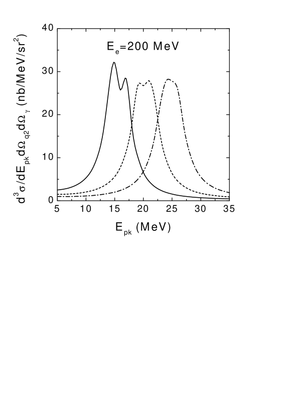
Figure 2: Differential cross section (5.36) for reaction $ep\to ep\gamma$ in the kinematics where proton bremsstrahlung dominates, see comments in the text. Proton scattering and photon emission angles are $\vartheta_{p}=-20.5^{0}$ (solid line), $\vartheta_{p}=-20.0^{0}$ (dashed line), $\vartheta_{p}=-19.5^{0}$ (dot-dashed line), and $\vartheta_{\gamma}=135^{0}$.

The differential cross section (5.36), shown by the graphs in Fig. 2, is the sum of the Bethe-Heitler ($\sigma_{ee}$), the interference ($\sigma_{ep}$), and the proton ($\sigma_{pp}$) terms [see (5.30)], where the symbol ($\sigma$) denotes a cross section of the form (5.36) with $\mid T\mid^{2}$ replaced by $Y_{ee}$, $Y_{ep}$, and $Y_{pp}$, respectively. Numerical calculations shown that in the entire range of proton kinetic energy studied, $5\leq E_{pk}\leq 35$ MeV, the ratios of the Bethe-Heitler term $\sigma_{ee}$ and the interference term $\sigma_{ep}$ to the term corresponding to proton emission $\sigma_{pp}$ are bounded by the values $\sigma_{ee}/\sigma_{pp}<0.02$ and $|\sigma_{ep}|/\sigma_{pp}<0.05$. The calculations carried out for another set of angles ($\vartheta_{\gamma}=135^{0}$ and $\vartheta_{p}=-20^{0}$) give results which are only insignificantly different: $\sigma_{ee}/\sigma_{pp}<0.05$ and $|\sigma_{ep}|/\sigma_{pp}<0.075$. Since these ratios are much smaller than unity, the main requirement (see Ref. 60) for separation of the background, which is mainly electron bremsstrahlung, is satisfied.

To explain the sensitivity of the reaction $ep\to ep\gamma$ to the proton polarizability we performed numerical calculations of the cross section (5.36) for the same set of angles ($\vartheta_{\gamma}=135^{0}$ and $\vartheta_{p}=-20^{0}$) for fixed sum of the electric and magnetic polarizabilities $\alpha_{p}+\beta_{p}=14$ but different values of the difference: (a) $\alpha_{p}-\beta_{p}=10$ and (b) $\alpha_{p}-\beta_{p}=6$. It turned out that the cross section (5.36) is about 8% larger for the smaller difference of polarizabilities. Therefore, in this kinematics the cross section for the reaction $ep\to ep\gamma$ is quite sensitive to the proton polarizability [65].

6 Emission of a linearly polarized photon by an electron in the reaction $ep\to ep\gamma$

Let us consider the emission of a linearly polarized photon by an electron in the reaction $ep\to ep\gamma$, taking into account the proton recoil and form factors. Our study will be limited to the contribution of the two Bethe-Heitler graphs (a) and (b) in Fig. 1, which corresponds to the matrix element (5.2). The contribution of the graph with VCS on a proton can be neglegted when the initial electrons have ultrarelativistic energies, and the photon and final electron are scattered at small forward angles ($\vartheta_{\gamma}\sim m/E_{e},\;\vartheta_{e}\sim m/E_{e},\;m/E_{e}\ll 1$).

We are interested in these effects for the following reasons. First, even though the Bethe-Heitler process has been studied earlier in the case of the emission of linearly polarized photons [69,70] and is widely used to obtain them at accelerators [71], up to now the proton recoil and form factors have not been accurately taken into account (in contrast to the unpolarized case). Second, as was shown in Ref. 72, the inclusion of these factors in the case of unpolarized photons leads to a strong change of the differential cross section for the Bethe-Heitler process. Since the polarization characteristic of the scattered radiation are expressed in terms of the differential cross section for the emission of an unpolarized photon (see below), it is clear that inclusion of the recoil and form factors is essential.

The covariant expression for the differential cross section for the Bethe-Heitler process (in the Born approximation) taking into account the proton recoil and form factors in the case of emission of a linearly polarized photon has been obtained by us in Ref. 73. It has the form

$$d\sigma_{BH}={\alpha^{3}\mid T_{e}\mid^{2}\delta^{4}(p_{1}+q_{1}-p_{2}-q_{2}-k)\over 2\pi^{2}\sqrt{(p_{1}q_{1})^{2}-m^{2}M^{2}}}\;\;{d^{3}\vec{p}_{2}\over 2p_{20}}\;{d^{3}\vec{q}_{2}\over 2q_{20}}{d^{3}\vec{k}\over 2\omega}\;\;,$$

$$\mid T_{e}\mid^{2}={4M^{2}\over q^{4}}\;(\;g_{e}^{2}\;Y_{I}^{~{}e}+\tau\;g_{m}^{2}\;Y_{II}^{~{}e}\;)\;,$$

$$Y_{I}^{~{}e}=2-{\lambda_{1}\over\lambda_{2}}-{\lambda_{2}\over\lambda_{1}}-{\tau\over 1-\tau}\;{(kq_{+})^{2}\over\lambda_{1}\lambda_{2}}+q^{2}\;(ea)^{2}+4\;(eA)^{2}\;,$$

$$Y_{II}^{~{}e}=-2-{\lambda_{1}\over\lambda_{2}}-{\lambda_{2}\over\lambda_{1}}+{\tau\over 1-\tau}\;{(kq_{+})^{2}\over\lambda_{1}\lambda_{2}}+(q^{2}+4m^{2})\;(ea)^{2}-4\;(eA)^{2}\;,$$

$$a={p_{1}\over\lambda_{1}}-{p_{2}\over\lambda_{2}}\;\;,\;\;A=b_{0}+{(b_{0}p_{2})p_{1}\over\lambda_{1}}-{(b_{0}p_{1})p_{2}\over\lambda_{2}}\;.$$

All the quantities entering into (6.1)-(6.5) are defined in the preceding section. Thus, the differential cross section for the Bethe-Heitler process in the case of emission of a linearly polarized photon $d\sigma_{BH}$ (6.1) naturally splits into the sum of two terms containing only the squares of the Sachs form factors and corresponding to the contribution of transition without ($\sim g_{e}^{2}\;Y_{I}^{~{}e}$) and with ($\sim\tau\;g_{m}^{2}Y_{II}^{~{}e}$) proton spin flip.

Let us discuss the properties of the 4-vector $a$, which is well known from the theory of emission of long-wavelength photons [10], and the 4-vector $A$. They both satisfy a condition which follows naturally from the requirement of gauge invariance:

$$a\;k=A\;k=0\;,$$

and, in addition, they are spacelike vectors: $a^{2}<0$ and $A^{2}<0$. This is easily verifed by using the 4-momentum conservation law and the explicit form of $a^{2}$ and $A^{2}$:

$$a^{2}=m^{2}\;\left({1\over\lambda_{1}}-{1\over\lambda_{2}}\right)^{2}+{r^{2}\over\lambda_{1}\lambda_{2}}\;,$$

$$A^{2}=1+{m^{2}\over 4M^{2}(1-\tau)}\;\left({q_{+}p_{1}\over\lambda_{2}}-{q_{+}p_{2}\over\lambda_{1}}\right)+{\tau\over 1-\tau}\;{q_{+}p_{1}\cdot q_{+}p_{2}\over\lambda_{1}\lambda_{2}}\;.$$

We note that the 4-vector $A$ was first introduced in Ref. 73.

Using the electron 4-momenta $p_{1}$ and $p_{2}$ and the photon 4-momenta $k$, we construct the 4-vectors of the photon linear polarization $e_{\parallel}$ and $e_{\perp}\;(e_{\parallel}k=e_{\perp}k=e_{\parallel}e_{\perp}=0$):

$$e_{\parallel}={(p_{2}k)p_{1}-(p_{1}k)p_{2}\over\rho^{{}^{\prime}}}\;,\;e_{\perp}={[p_{1}\cdot p_{2}]^{\times}k\over\rho^{{}^{\prime}}}\;,$$

where $\rho^{{}^{\prime}}$ is determined from the normalization conditions: $e_{\parallel}^{2}=e_{\perp}^{2}=-1$. Then the degree of photon linear polarization will be given by the following expressions [73]:

$$P_{\gamma}={\mid T_{\perp}\mid^{2}-\mid T_{\parallel}\mid^{2}\over\mid T_{\perp}\mid^{2}+\mid T_{\parallel}\mid^{2}}={A_{1}\over A_{2}}\;,$$

where

$$A_{1}={16\;M^{2}\over q^{4}}\;(g_{e}^{2}\;A_{11}+\tau\;g_{m}^{2}\;A_{12})\;,$$

$$A_{2}={8\;M^{2}\over q^{4}}\;(g_{e}^{2}\;Y_{1}+\tau\;g_{m}^{2}\;Y_{2})\;,$$

$$A_{11}=A^{2}+\tau\;M^{2}\;a^{2}+2(e_{\perp}b_{0})^{2}\;,$$

$$A_{12}=-A^{2}+\tau\;M^{2}\;a^{2}-2(e_{\perp}b_{0})^{2}+m^{2}\;a^{2}\;,$$

$$(e_{\perp}b_{0})^{2}=-\;{4(SD)^{2}\over M^{2}(1-\tau)a^{2}\lambda_{1}^{2}\lambda_{2}^{2}}\;,$$

$$SD=1/2\;\epsilon_{\mu\nu\rho\sigma}(p_{1})^{\mu}(p_{2})^{\nu}(q_{1})^{\rho}(q_{2})^{\sigma}\;,$$

$$Y_{1}=2-{\lambda_{1}\over\lambda_{2}}-{\lambda_{2}\over\lambda_{1}}-{\tau\over 1-\tau}\;{(kq_{+})^{2}\over\lambda_{1}\lambda_{2}}-2\;\tau M^{2}\;a^{2}-2\;A^{2}\;,$$

$$Y_{2}=-2-{\lambda_{1}\over\lambda_{2}}-{\lambda_{2}\over\lambda_{1}}+{\tau\over 1-\tau}\;{(kq_{+})^{2}\over\lambda_{1}\lambda_{2}}-2\;\tau\;M^{2}\;a^{2}+2\;A^{2}-2m^{2}\;a^{2}\;.$$

It is easy to check that $A_{2}$ (6.11) coincides with the expression for $Y_{ee}$ (5.31) determining the Bethe-Heitler cross section in the case of unpolarized particles: $A_{2}=Y_{ee}$, and also that $Y_{1}=Y_{I}$ and $Y_{2}=Y_{II}$ [see (5.32) and (5.33)].

Therefore, owing to the factorization of the squares of the form factors $g_{e}$ and $g_{m}$ and also the use of the 4-vectors $a$ and $A$ (6.5), the differential cross section for the Bethe-Heitler process in both the cases of linearly polarized photon (6.2) and unpolarized photon (6.11), (5.31), can be written in a rather compact form.

Let us integrate Eq. (6.1) over $d^{3}\vec{q}_{2}$ and $dp_{20}$ in the rest frame of the initial proton, $q_{1}=(M,0)$. As a result, we find:

$${d\sigma_{BH}\over d\omega\;d\Omega_{\gamma}\;d\Omega_{e}}={\alpha^{3}\;\omega\over(2\pi)^{2}}\;{|\vec{p}_{2}|\over|\vec{p}_{1}|}\;{|T|^{2}\over q^{4}\;}\;,$$

$$|T|^{2}=g_{e}^{2}\;Y_{I}^{~{}e}+\tau\;g_{m}^{2}\;Y_{II}^{~{}e}\;.$$

Let us consider the limit of the cross section (6.18) when the proton is a point (structureless) particle with infinite mass, i.e., we assume that $g_{e}=g_{m}=1$ and $q_{2}=(M,\vec{q})\simeq(M,0)$, where $\vec{q}=\vec{p}_{1}-\vec{p}_{2}-\vec{k}$ is the momentum transferred to the proton. In this limit ($M\to\infty$), $E_{kp}=\vec{q}~{}^{2}/2M\to 0,\;\vec{q}/2M\to 0$, and $b_{0}=(1,\vec{q}/2M)\simeq(1,0)$. We choose the Coulomb gauge for the photon polarization vectors: $e=(0,\vec{e})$, as a result of which we find

$$eb_{0}=0,\;ea={p_{1}e\over\lambda_{1}}-{p_{2}e\over\lambda_{2}},\;eA=p_{20}\;{p_{1}e\over\lambda_{1}}-p_{10}\;{p_{2}e\over\lambda_{2}},\;\tau(q_{+}k)^{2}=\omega^{2}q^{2}\;.$$

Using these expressions to take an limit in (6.19), we obtain:

$$|T|^{2}=2-{\lambda_{1}\over\lambda_{2}}-{\lambda_{2}\over\lambda_{1}}-{\omega^{2}q^{2}\over\lambda_{1}\lambda_{2}}+q^{2}\;(ea)^{2}+4\;(eA)^{2}\;,$$

or, in expanded form,

$$|T|^{2}=2-{\lambda_{1}\over\lambda_{2}}-{\lambda_{2}\over\lambda_{1}}-{\omega^{2}q^{2}\over\lambda_{1}\lambda_{2}}+\;(\;4p_{20}^{2}+q^{2}\;)\left({p_{1}e\over\lambda_{1}}\right)^{2}$$

$$+\;(\;4p_{10}^{2}+q^{2}\;)\left({p_{2}e\over\lambda_{2}}\right)^{2}-2\;(\;4p_{10}p_{20}+q^{2}\;)\;{p_{1}e\cdot p_{2}e\over\lambda_{1}\lambda_{2}}\;.$$

The expressions (6.18) and (6.21) for the differential cross section for the Bethe-Heitler process $d\sigma_{BH}/d\omega/d\Omega_{\gamma}/d\Omega_{e}$ in the limit where the proton is an infinitely heavy, structureless particle coincide with the analogous expressions of Ref. [69].

7 Virtual-photon polarization in the reaction
$ep\to ep\gamma\;(ep\to eX)$

The reaction $ep\to ep\gamma$ and VCS on a proton have recently become interesting not only at low and intermediate energies [60], but also at high electron energies and 4-momenta transferred to the proton [63,74-77]. The VCS process offers greater possibilities for studying hadronic structure than the RCS process, because in it the energy and three-momentum transferred to the target can be varied independently. These attractive properties of VCS have led to the suggestion that it be used for experimental study of the nucleon structure [74,75] and have made it necessary to perform a thorough theoretical study of the reaction $ep\to ep\gamma$ (including the use of the noncovariant method of calculating helicity amplitudes; (see Refs. 63, 76 and 77 and references therein)). To calculate VCS on a proton, it is necessary to know the hadron ($W_{\mu\nu}$) and lepton ($L_{\mu\nu}$) tensors [63,78]:

$$L_{\mu\nu}=J_{\mu}J_{\nu}^{*},~{}~{}J_{\mu}=\overline{u}(p_{2})\gamma_{\mu}u(p_{1})\;,$$

where $u(p_{i})$ are electron bispinors, $\overline{u}(p_{i})u(p_{i})=2m$, and $m$ is the electron mass ($i=1,2$). The interpretation of the results is considerably simplified if the tensor $L_{\mu\nu}$ is expressed in terms of the longitudinal and transverse polarization vectors of the virtual photon. The corresponding expressions can be found in Refs. 63 and 78. However, they have two defects: (1) the electron mass is neglegted, which is of course justified at ultrarelativistic electron energies and large squared 4-momentum of the virtual photon; (2) they have a noncovariant form. A lepton tensor free of these defects was constructed in Ref. 79.

Let us consider the question of the polarization state of a virtual $\gamma$ with 4-momentum $r=p_{1}-p_{2}$ which is exchanged between the electron and proton in the reaction $ep\to ep\gamma$ (see Fig. 1c). Using the vectors of the orthonormal basis $a_{A}$ (5.9) ($A=(0,1,2,3)$):

$$a_{0}=p_{+}/\sqrt{p_{+}^{2}}\;,\;a_{3}=p_{-}/\sqrt{-p_{-}^{2}}\;,\;a_{2}=[a_{0}\cdot a_{3}]^{\times}q_{1}/\rho\;,\;a_{1}=[a_{0}\cdot a_{3}]^{\times}a_{2}\;,$$

$$p_{\pm}=p_{2}\pm p_{1}\;,\;a_{2}q_{1}=0\;,\;a_{1}^{2}=a_{2}^{2}=a_{3}^{2}=-a_{0}^{2}=-1\;,$$

which satisfy the completeness relation

$$a_{0}\cdot a_{0}-a_{1}\cdot a_{1}-a_{2}\cdot a_{2}-a_{3}\cdot a_{3}=g\;,$$

we construct the 4-vectors of the longitudinal ($e_{3}$) and transverse ($e_{1},\;e_{2}$) polarization of a virtual photon with 4-momentum $r$ (Ref. 79):

$$e_{1}={[a_{0}\cdot a_{1}]q_{1}\over\sqrt{(a_{3}q_{1})^{2}+q_{1}^{2}}}\;,\;e_{2}=a_{2}={[a_{0}\cdot a_{3}]^{\times}q_{1}\over\rho}\;,\;e_{3}={(1+a_{3}\cdot a_{3})q_{1}\over\sqrt{(a_{3}q_{1})^{2}+q_{1}^{2}}}\;,$$

where

$$\rho^{2}=(a_{1}q_{1})^{2}={2p_{1}p_{2}\cdot p_{1}q_{1}\cdot p_{2}q_{1}-M^{2}((p_{1}p_{2})^{2}-m^{4})-m^{2}((p_{1}q_{1})^{2}+(p_{2}q_{1})^{2})\over(p_{1}p_{2})^{2}-m^{4}}.$$

It is easily verifed that the 4-vectors $e_{i}\;(i=1,2,3)$ are orthogonal to each other ($e_{i}e_{j}=0,\;i\neq j$), and also that $e_{i}r=e_{i}a_{3}=0$ and $e_{1}^{2}=e_{2}^{2}=-e_{3}^{2}=-1$. The 4-vectors $e_{i}$ (7.5) are not changed when the auxiliary 4-vector $q_{1}$ is replaced by $q_{1}+p_{1}-p_{2}=q_{2}+k$ [because $p_{1}-p_{2}=r=-2ya_{3}$, where $y=\sqrt{-r^{2}}/2$, and because the vectors $a_{A}$ (7.2) are orthogonal]. For this reason, study of the virtual-photon polarization vectors $e_{i}$ (7.5) in the rest frame of the incident proton or in the c.m. frame of the final proton and photon is equivalent and leads to the usual expressions. Here we shall restrict ourselves to the rest frame of the incident proton [$q_{1}=(M,0,0,0)]$, where the 4-vectors $e_{i}$ have the form:

$$e_{1}=(0,1,0,0),\;e_{2}=(0,0,1,0),\;e_{3}={1\over\sqrt{-r^{2}}}(\mid\vec{r}\mid,r_{0}\vec{n}_{3})\;.$$

Here $\vec{n}_{3}$ is a unit vector directed along $\vec{r}\;(\vec{n}_{3}^{~{}2}=1)$, and $r_{0}$ is the time component of the 4-vector $r=(r_{0},\vec{r})$.

The four mutually orthogonal vectors $e_{1},e_{2},e_{3}$, and $a_{3}$ also satisfy the completeness relation:

$$e_{3}\cdot e_{3}-e_{1}\cdot e_{1}-e_{2}\cdot e_{2}-a_{3}\cdot a_{3}=g\;,$$

which allows $a_{0}$ and $a_{1}$ to be expressed in terms of $e_{1}$ and $e_{3}$:

$$a_{1}=\alpha e_{3}-\beta e_{1}\;,\;a_{0}=\beta e_{3}-\alpha e_{1}\;,\;\beta^{2}=1+\alpha^{2}\;\;,$$

$$\alpha=e_{3}a_{1}=a_{0}e_{1}={a_{1}q_{1}\over\sqrt{(a_{3}q_{1})^{2}+q_{1}^{2}}}\;,\;\beta=e_{1}a_{1}=e_{3}a_{0}={a_{0}q_{1}\over\sqrt{(a_{3}q_{1})^{2}+q_{1}^{2}}}\;.$$

In the DSB (4) the matrix elements of the electron current have the form of (5.18):

$$(J^{\delta,\delta}_{e})_{\mu}=2m(a_{0})_{\mu},\;(J^{-\delta,\delta}_{e})_{\mu}=-2\delta y\;(a_{\delta})_{\mu},$$

where $a_{\pm\delta}=a_{1}\pm i\delta a_{2},\;\delta=\pm 1$. Let us write them in terms of the 4-vectors $e_{i}$ (7.5) (Ref. 79):

$$(J^{\delta,\delta}_{e})_{\mu}=2m\;(\beta e_{3}-\alpha e_{1})_{\mu}\;,\;(J^{-\delta,\delta}_{e})_{\mu}=-2\delta y\;(\alpha e_{3}-\beta e_{1}+i\delta e_{2})_{\mu}\;.$$

Therefore, for transition without electron spin flip $(J^{\delta,\delta}_{e})$ the virtual-photon polarization vector is a superposition of the longitudinal ($\beta e_{3}$) and transverse linear ($-\alpha e_{1}$) polarizations, while for transition with spin flip $(J^{-\delta,\delta}_{e})$ it is a superposition of the longitudinal ($\alpha e_{3}$) and transverse elliptical [$e_{\delta}=(0,\vec{e}_{\delta})=-\beta e_{1}+i\delta e_{2}$] polarizations. Here the state of a photon with elliptical polarization vector $e_{\delta}=(0,\vec{e}_{\delta})$ will have degree of linear polarization (equal to the ratio of the difference and sum of the squared semiaxes [57]) [79]:

$$\kappa_{\gamma}={\beta^{2}-1\over\beta^{2}+1}={\alpha^{2}\over\beta^{2}+1}\;.$$

Inverting this relation, we obtain:

$$\beta^{2}={1+\kappa_{\gamma}\over 1-\kappa_{\gamma}}\;\;,\;\alpha^{2}={2\kappa_{\gamma}\over 1-\kappa_{\gamma}}\;\;.$$

Now we find the squared moduli of the vectors $\vec{e}_{\delta}$ and $\vec{a}_{\delta}$:

$$\mid\vec{e}_{\delta}\mid^{2}=1+\beta^{2}={2\over 1-\kappa_{\gamma}}\;,\;\mid\vec{a}_{\delta}\mid^{2}=(1+\beta^{2})\;(1+\kappa_{L})\;,$$

$$\kappa_{L}=\kappa_{\gamma}\vec{e}_{3}^{~{}2}=\kappa_{\gamma}{r_{0}^{2}\over(-r^{2})}\;,\;\vec{e}_{3}^{~{}2}={r_{0}^{2}\over(-r^{2})}\;.$$

We introduce the normalized vectors $\vec{e}_{\delta}~{}^{\prime}$ and $\vec{a}_{\delta}~{}^{\prime}$:

$$\vec{e}_{\delta}~{}^{\prime}={\vec{e}_{\delta}\over\sqrt{1+\beta^{2}}}=\sqrt{{1-\kappa_{\gamma}\over 2}}\;\vec{e}_{\delta}\;,\;|\vec{e}_{\delta}^{~{}^{\prime}}|^{2}=1\;.$$

$$\vec{a}_{\delta}~{}^{\prime}={\vec{a}_{\delta}\over\sqrt{1+\beta^{2}}}=\sqrt{{1-\kappa_{\gamma}\over 2}}\;\vec{a}_{\delta}\;,\;|\vec{a}_{\delta}^{~{}^{\prime}}|^{2}=1+\kappa_{\gamma}\vec{e}_{3}^{~{}2}=1+\kappa_{L}\;,$$

Therefore, the elliptical-polarization vector $\vec{e}_{\delta}$ of a virtual photon can be normalized to unity ($|\vec{e}_{\delta}~{}^{\prime}|^{2}=1$), but the presence of a longitudinal polarization makes this normalization impossible for the total vector $\vec{a}_{\delta}~{}^{\prime}$ simultaneously. The quantity $\kappa_{L}$ (7.15) corresponding to the inequality $|\vec{a}_{\delta}~{}^{\prime}|^{2}=1+\kappa_{L}\neq 1$ has the meaning of the degree of longitudinal polarization of a virtual photon emitted in a transition with electron spin flip. In the ultrarelativistic limit, when the electron mass can be neglected, the quantities $\kappa_{\gamma}$ and $\kappa_{L}$ will be interpreted as the total degrees of linear and longitudinal polarization of the virtual photon. In this (massless) case we have:

$$(a_{3}q_{1})^{2}+q_{1}^{2}=-M^{2}\;{\vec{r}^{~{}2}\over r^{2}}\;,\;(a_{1}q_{1})^{2}=M^{2}\;ctg^{2}\vartheta/2\;,$$

$$\kappa_{\gamma}^{-1}=1-2\;{\vec{r}^{~{}2}\over r^{2}}\;tg^{2}\vartheta/2\;,$$

where $\vartheta$ is the angle between the vectors $\vec{p}_{1}$ and $\vec{p}_{2}$. Equation (7.19) for $\kappa_{\gamma}$ coincides with the result of Ref. 78.

The vector $\vec{a}_{\delta}~{}^{\prime}$ (7.17) can also be written as

$$\vec{a}_{\delta}~{}^{\prime}=\sqrt{\kappa_{L}}\;\vec{n}_{3}-\sqrt{{1+\kappa_{\gamma}\over 2}}\;\vec{e}_{1}+i\delta\;\sqrt{{1-\kappa_{\gamma}\over 2}}\;\vec{e}_{2}\;\;,$$

which makes it easy to construct the polarization density matrix for a virtual photon in the massless limit (both in the polarized case, which for massless particles is helical polarization, and in the unpolarized case; see Ref. 78).

To obtain the complete expression for $\kappa_{\gamma}$ and $\kappa_{L}$ arising from the contributions of the matrix elements both without and with spin flip, we construct the lepton tensor averaged over electron spin states. Using the matrix elements (7.10) and (7.11), this can be done fairly simply [79]:

$$\overline{L}_{\mu\nu}=4m^{2}\;(a_{0})_{\mu}(a_{0})_{\nu}+4y^{2}\;((a_{1})_{\mu}(a_{1})_{\nu}+(a_{2})_{\mu}(a_{2})_{\nu})\;.$$

Using the completeness condition (7.3) and gauge invariance, the tensor $\overline{L}_{\mu\nu}$ can be written as

$$\overline{L}_{\mu\nu}=4x^{2}\;(a_{0})_{\mu}(a_{0})_{\nu}-4y^{2}\;g_{\mu\nu}\;,$$

where $x^{2}=m^{2}+y^{2}$. The tensor $\overline{L}_{\mu\nu}$ (7.22) can be used to reduce the calculation of the contribution of graphs with VCS on a proton to the cross section for the reaction $ep\to ep\gamma$ to calculation of the trace of a product of tensors:

$$Y_{pp}=\overline{L}_{\mu\nu}\;W_{\mu\nu}\;,\;W_{\mu\nu}=V_{\mu}V_{\nu}^{\ast}\;,\;V_{\mu}=\overline{u}(q_{2})\;M_{\mu\nu}e^{\nu}\;u(q_{1})\;{1\over r^{2}}\;.$$

Let us express the tensor $\overline{L}_{\mu\nu}$ (7.21) in the terms of the virtual-photon polarization vectors $e_{i}$ (7.5). As a result, it naturally breaks up into the sum of three terms corresponding to the contributions of transverse ($L_{T}$) and longitudinal ($L_{L}$) states and their interference ($L_{LT}$) [79]:

$$\overline{L}=4y^{2}\;(L_{T}\;+\;L_{L}\;+\;L_{LT}\;)\;,~{}~{}~{}~{}~{}~{}~{}~{}~{}~{}~{}~{}$$

$$L_{T}=e_{1}\cdot e_{1}\;(\beta^{2}+\alpha^{2}m^{2}/y^{2})+e_{2}\cdot e_{2}\;,~{}~{}$$

$$L_{L}=e_{3}\cdot e_{3}\;(\alpha^{2}+\beta^{2}m^{2}/y^{2})\;,~{}~{}~{}~{}~{}~{}~{}~{}~{}~{}~{}~{}$$

$$~{}~{}~{}~{}~{}L_{LT}=-\;(e_{1}\cdot e_{3}+e_{3}\cdot e_{1})\;\alpha\beta\;(1+m^{2}/y^{2})\;.$$

Then the total degree of linear polarization of the virtual photon will be given by

$$\kappa_{\gamma}^{\prime}={\beta^{2}+\alpha^{2}m^{2}/y^{2}-1\over\beta^{2}+\alpha^{2}m^{2}/y^{2}+1}={\alpha^{2}\over\beta^{2}+1-2m^{2}/x^{2}}\;.$$

Since $\alpha$ and $\beta$ are the same in Eqs. (7.12) and (7.28) [see (7.9)], the inclusion of the electron mass in the ultrarelativistic limit will lead only to a slight increase of $\kappa_{\gamma}$ [79]:

$$\kappa_{\gamma}^{\prime}\simeq\kappa_{\gamma}\left(1+{2m^{2}\over x^{2}(1+\beta^{2})}\right)\;.$$

Inverting the relation in (7.28), we find

$$\beta^{2}+\alpha^{2}m^{2}/y^{2}={1+\kappa_{\gamma}^{\prime}\over 1-\kappa_{\gamma}^{\prime}}\;,\;\alpha^{2}+\beta^{2}m^{2}/y^{2}={2\kappa_{\gamma}^{\prime}\over 1-\kappa_{\gamma}^{\prime}}+{m^{2}\over y^{2}}\;.$$

We can separate the completely polarized and unpolarized parts in the transverse tensor $L_{T}$ (7.25):

$$L_{T}=e_{1}\cdot e_{1}\,(\beta^{2}+\alpha^{2}m^{2}/y^{2}-1)+e_{1}\cdot e_{1}+e_{2}\cdot e_{2}\,={2\over 1-\kappa_{\gamma}^{\prime}}\,(\,\kappa_{\gamma}^{\prime}\,e_{1}\cdot e_{1}+(1-\kappa_{\gamma}^{\prime})\,(e_{1}\cdot e_{1}+e_{2}\cdot e_{2})/2\,)\,.$$

Therefore, the virtual-photon polarization density matrix $\rho_{ij}$ is obtained from the tensor $\overline{L}_{ij}$ (7.24) just as in the massless case (see Ref. 78):

$$\rho_{ij}=(1-\kappa_{\gamma}^{\prime})\;\overline{L}_{ij}/8y^{2}\;.$$

For the degree of longitudinal polarization of the virtual photon we then obtain:

$$\kappa_{L}^{\prime}={r_{0}^{2}\over(-r^{2})}\kappa_{\gamma}^{\prime}\;\left(1+{m^{2}\over y^{2}}\;{(1-\kappa_{\gamma}^{\prime})\over 2\kappa_{\gamma}^{\prime}}\right)\;.$$

The expressions (7.28) and (7.33) for $\kappa_{\gamma}^{\prime}$ and $\kappa_{L}^{\prime}$ with $m=0$ obviously become $\kappa_{\gamma}$ and $\kappa_{L}$ of (7.12) and (7.15).

We conclude by noting that the region of applicability of the tensor $\overline{L}_{\mu\nu}$ (7.24) is not limited to only VCS on a proton. Since in fixed-target experimets the charged-lepton scattering at available energies is mainly determined by virtual photon exchange, the tensor $\overline{L}_{\mu\nu}$ (7.24) can also be used to study deep-inelastic electron scattering ($e^{\pm}p\to e^{\pm}X$), and muon scattering ($\mu^{\pm}p\to\mu^{\pm}X$), where inclusion of the mass is more important.

8 Compton back-scattering of the photons of a circularly
polarized laser wave on a beam of ultrarelativistic,
longitudinally polarized electrons

It was shown in Refs. 80 and 81 that, using existing (SLC) and planned (VLEPP) accelerators with colliding $e^{+}e^{-}$ beams, it is possible to obtain colliding $\gamma e$ and $\gamma\gamma$ beams of roughly the same energy and luminosity as the original $e^{+}e^{-}$ beams. It have been suggested that the intense beams of hard $\gamma$ rays needed for this be obtained from the Compton back-scattering (CBS) of a powerful laser flash focused on the electron beam [82]. For a sufficiently powerful flash in the conversion region [81], processes with simultaneous absorption of several laser photons from the wave become important:

$$e^{-}+n\;\gamma_{0}\rightarrow e^{-}+\gamma\;,\;n\geq 1\;,$$

$$\gamma+s\;\gamma_{0}\rightarrow e^{+}+e^{-}\;,\;s\geq 1\;.$$

The first of these nonlinear processes leads to broadering of the spectrum of high-energy photons [83], and the second effectively lowers the $e^{+}e^{-}$-pair production threshold [84].

The process (8.1) and (8.2) were studied systematically in Ref. 85. In Ref. 16 they were studied from the view-point of providing sources of polarized $\gamma$ and $e^{+}e^{-}$ beams. The phenomena arising in collisions of polarized electrons with the photons of a circularly polarized electromagnetic wave were analyzed in Ref. 86. Nonlinear effects were studied not only for $\xi^{2}<1$, but also for $\xi^{2}\geq 1$. Here $x^{2}$ is the wave intensity parameter:

$$\xi^{2}=n_{\gamma}\left({4\pi\alpha\over m^{2}\omega}\right)\;,$$

where $n_{\gamma}$ is the photon density in the wave and $\omega$ is the photon energy, $\alpha$ is the fine structure constant, $m$ is the electron mass. The emission spectra at high intensities ($\xi^{2}\geq 1$) were first calculated numerically in Ref. 83, but the particle polarization was not taken into account.

Recently at the SLAC accelerator a series of experiments [87] are being performed for $\xi\sim 1$ to verify nonlinear QED. This has become possible owing to the use of supershort, strongly focused laser pulses. The region of nonlinear effects for $\xi^{2}\geq 1$ is very important here, and it is of great interest because emission processes due to simultaneous absorption of a large number of photons from the wave become important, and the probabilities for these processes are essentially nonlinear functions of the field strength.

As a rule, in the literature the laser wave is described as the field of a planar electromagnetic wave [85,86]. The applicability of this model in strong fields has been studied in Ref. 88.

According to Ref. 10, the $S$-matrix element for the transition of an electron from the state $\psi_{p}=\psi^{\delta}(p,s)$ to the state $\psi_{p^{\prime}}=\psi^{\pm\delta}(p^{\prime},s^{\prime})\;,(\delta=\pm 1)$, with the emission of a photon of 4-momentum $k^{\prime}=(\omega^{\prime},\vec{k}^{\prime})$ and circular-polarization vector $e_{\lambda^{\prime}}$ is given by

$$S_{fi}=-i\;e\;\int\overline{\psi}_{p^{\prime}}\;\hat{e}^{\ast}_{\lambda^{\prime}}\;\psi_{p}\;exp(ik^{\prime}x)\;(2\omega^{\prime})^{-1/2}\;d^{4}x\;,$$

where $\psi_{p}$ and $\overline{\psi}_{p^{\prime}}$ are the exact wave functions of electrons in the field of a circularly polarized electromagnetic wave, corresponding to the vector potential

$$A=a_{1}\cos(kx)+\lambda a_{2}\sin(kx),\;\lambda=\pm 1.$$

Here $k$ is the wave vector, $k^{2}=0,a_{1}k=a_{2}k=a_{1}a_{2}=0,a_{1}^{2}=a_{2}^{2}=a^{2}$, and $\lambda$, $\lambda^{{}^{\prime}}$ are helicities of a laser and emission photons. The explicit form of the matrix elements (8.4) in the DSB was obtained in Refs. 38 and 86:

$$S_{fi}=-\;{ie\;(4\pi)^{1/2}\over(2\omega^{\prime}\;2q_{0}\;2q_{0}^{\prime})^{1/2}}\;\;\sum_{n=1}^{\infty}\;M^{~{}(n)}_{\pm\delta,\delta}\;(2\pi)^{4}\;\delta^{4}(nk+q-q^{\prime}-k^{\prime})\;,$$

$$M^{~{}(n)}_{-\delta,\delta}=-\;\;{1\over 2}\;\;\lambda^{\prime}\;(-\lambda)^{n}\;\xi\;\Biggl{\{}-\;{2(1-u/u_{n})\over\sqrt{vv^{\prime}-1}}\;(J_{n-1}+J_{n+1})\Biggr{.}$$

$$+\Biggl{.}\;{1\over 2(u+1)}\;\left({(u+2)^{2}\over\sqrt{vv^{\prime}+1}}-\delta\lambda^{\prime}\;{u^{2}\over\sqrt{vv^{\prime}-1}}\right)\;J_{n+\lambda\lambda^{\prime}}\Biggr{\}}\;,$$

$$~{}M^{~{}(n)}_{\delta,\delta}=-\;\;{1\over 2}\;\lambda^{\prime}\;(-\lambda)^{n}\;\xi\;\sqrt{{u\over u_{n}}\;\left(1-{u\over u_{n}}\right)}\;\left({u+2\over u}\sqrt{{vv^{\prime}-1\over vv^{\prime}+1}}-\delta\lambda^{\prime}\right)$$

$$\times\left(\sqrt{{vv^{\prime}-1\over 1+\xi^{2}}}(J_{n-1}+J_{n+1})-{uu_{n}\sqrt{1+\xi^{2}}\over 2(u+1)\sqrt{vv^{\prime}-1}}\;J_{n+\lambda\lambda^{\prime}}\right)\;,$$

where

$$q=p+{\xi^{2}m^{2}\over 2kp}\;k\;,\;q^{\prime}=p^{\prime}+{\xi^{2}m^{2}\over 2kp^{\prime}}\;k\;,\;q^{2}=q^{\prime 2}=m_{\ast}^{2}=m^{2}\;(1+\xi^{2})\;,$$

$$u={kk^{\prime}\over kp^{\prime}}\;,\;u_{n}={2nkp\over m_{\ast}^{2}}\;,2(vv^{\prime}-1)={uu_{n}\over u+1}\left(1+\xi^{2}\;\left(1-{u\over u_{n}}\right)\right)\;,$$

$$J_{n+\lambda\lambda^{\prime}}={(1+\lambda\lambda^{\prime})\over 2}\;J_{n+1}+{(1-\lambda\lambda^{\prime})\over 2}\;J_{n-1}\;,\;nk+q=k^{\prime}+q^{\prime}\;,$$

$$z_{n}={2n\xi\over\sqrt{1+\xi^{2}}}\;\sqrt{{u\over u_{n}}\left(1-{u\over u_{n}}\right)}\;\;.$$

Here $M^{~{}(n)}_{\delta,\delta}$ and $M^{~{}(n)}_{-\delta,\delta}$ are the emission amplitudes of the $n$-th harmonic corresponding to transitions without and with electron spin flip, $q$ and $q^{\prime}$ are the electron quasimomentum 4-vectors, $q=(q_{0},\vec{q}),\;q^{\prime}=(q^{\prime}_{0},\,\vec{q}~{}^{\prime})$, and $J_{n}$ are the $n$-th-order Bessel function of argument $z_{n}$. It is easily verifed that the amplitudes $M^{~{}(n)}_{\pm\delta,\delta}$ have the following kinematical features. For $u=u_{n}$ and $n>1$ they vanish [$M^{~{}(n)}_{\pm\delta,\delta}(u=u_{n})=0]$. The reason for this behavior of the amplitudes will be explained below. Knowledge of the diagonal amplitudes (8.7) and (8.8) allows transformation to the helicity amplitudes (see Ref. 86). As a result, we obtain the following expressions for the differential cross section of the hard photon emission by an electron in the field of circularly polarized electromagnetic wave [86]:

$${d\sigma_{c}\over du}={\pi\alpha^{2}\over xm^{2}\xi^{2}(u+1)^{2}}\;\sum_{n=1}^{\infty}\;(\;F_{1n}+\lambda\lambda_{e}\;F_{2n}+\lambda\lambda^{\prime}\;F_{3n}+\lambda_{e}\lambda^{\prime}\;F_{4n}\;)\;,$$

$$F_{1n} = -4\;J_{n}^{2}+\xi^{2}\;\left(2+{u^{2}\over u+1}\right)\;(J_{n-1}^{2}+J_{n+1}^{2}-2J_{n}^{2})\;,$$

$$F_{2n} = \xi^{2}\;{(2+u)u\over u+1}\;\left(1-2{u\over u_{n}}\right)\;(J_{n-1}^{2}-J_{n+1}^{2})\;,$$

$$F_{3n}=\xi^{2}\;\left(2+{u^{2}\over u+1}\right)\;\left(1-2\;{u\over u_{n}}\right)\;(J_{n-1}^{2}-J_{n+1}^{2})\;,~{}~{}~{}~{}~{}~{}~{}$$

$$~{}~{}~{}F_{4n}={u\over u+1}\;(-4\;J_{n}^{2}+\xi^{2}\;(2+u)\;(J_{n-1}^{2}+J_{n+1}^{2}-2J_{n}^{2})\;)\;,$$

here $x=2kp/m^{2}$, $\lambda_{e}$ is the helicity of the electron, $\lambda_{e}=\pm 1$. The expression inside the summation in (8.10) determines the emission probability of the $n$-th harmonic when the polarization states of the laser and the emitted photons and also the initial state of the electron are helicity states. For $\xi^{2}=0$ Eq. (8.10) coincides with the result of Ref. 89.

Using (8.10), the degree of circular polarization of a photon in the final state $\lambda_{f}$ is defined as

$$\lambda_{f}=\sum_{n=1}^{\infty}\;(\lambda\;F_{3n}+\lambda_{e}\;F_{4n}\;)\;/\;\sum_{n=1}^{\infty}\;(\;F_{1n}+\lambda\lambda_{e}\;F_{2n}\;)\;.$$

For $\xi^{2}<1$ only the first few harmonics dominate in the cross section (8.10) for the process (8.1). We expand the expressions (8.11) in the parameter $\Delta=\xi^{2}/(1+\xi^{2})$, expanding only the Bessel functions and using the exact expressions for the $u_{n}$. As a result, for the first three harmonics we have [86]:

$${F_{11}\over\xi^{2}} = 2+{u^{2}\over 1+u}-4{u\over u_{1}}\left(1-{u\over u_{1}}\right)+4\Delta{u\over u_{1}}\left(1-{u\over u_{1}}\right)\left[1+{u^{2}\over 1+u}\right.~{}~{}~{}$$

$$- \left.{u\over u_{1}}\left(1-{u\over u_{1}}\right)\right]+\Delta^{2}{u^{2}\over u_{1}^{2}}\left(1-{u\over u_{1}}\right)^{2}\left[{7\over 2}+{15\over 4}{u^{2}\over 1+u}-{5\over 3}{u\over u_{1}}\left(1-{u\over u_{1}}\right)\right],~{}~{}~{}$$

$${F_{21}\over\xi^{2}}={u(2+u)\over 1+u}\left(1-2{u\over u_{1}}\right)\left[1-2\Delta{u\over u_{1}}\left(1-{u\over u_{1}}\right)+{5\over 4}\Delta^{2}{u^{2}\over u_{1}^{2}}\left(1-{u\over u_{1}}\right)^{2}\right],~{}~{}~{}$$

$${F_{31}\over\xi^{2}} = \left(2+{u^{2}\over 1+u}\right)\left(1-2{u\over u_{1}}\right)\left[1-2\Delta{u\over u_{1}}\left(1-{u\over u_{1}}\right)+{5\over 4}\Delta^{2}{u^{2}\over u_{1}^{2}}\left(1-{u\over u_{1}}\right)^{2}\right],$$

$${F_{41}\over\xi^{2}} = {u\over 1+u}\biggl{\{}2+u-4{u\over u_{1}}\left(1-{u\over u_{1}}\right)-4\Delta{u\over u_{1}}\left(1-{u\over u_{1}}\right)\left[1+u-{u\over u_{1}}\left(1-{u\over u_{1}}\right)\right]\biggr{.}$$

$$+ \Delta^{2}{u^{2}\over u_{1}^{2}}\left(1-{u\over u_{1}}\right)^{2}\left[{7\over 2}+{15\over 4}u-{5\over 3}{u\over u_{1}}\left(1-{u\over u_{1}}\right)\right]\biggr{\}},$$

for the first harmonic;

$$F_{12} = 4\xi^{2}\Delta{u\over u_{2}}\left(1-{u\over u_{2}}\right)\biggl{\{}2+{u^{2}\over 1+u}-4{u\over u_{2}}\left(1-{u\over u_{2}}\right)\biggr{.}\quad~{}~{}~{}~{}~{}~{}$$

$$- 2\biggl{.}~{}\Delta{u\over u_{2}}\left(1-{u\over u_{2}}\right)\left(4+{3u^{2}\over 1+u}-{16\over 3}{u\over u_{2}}\left(1-{u\over u_{2}}\right)\right)\biggr{\}},$$

$$\hskip 91.04872ptF_{22}=4\xi^{2}\Delta{u\over u_{2}}\left(1-{u\over u_{2}}\right){u(2+u)\over 1+u}\left(1-2{u\over u_{2}}\right)\left[1-4\Delta{u\over u_{2}}\left(1-{u\over u_{2}}\right)\right],$$

$$\hskip 56.9055pt~{}~{}F_{32} = 4\xi^{2}\Delta{u\over u_{2}}\left(1-{u\over u_{2}}\right)\left(2+{u^{2}\over 1+u}\right)\left(1-2{u\over u_{2}}\right)\left[1-4\Delta{u\over u_{2}}\left(1-{u\over u_{2}}\right)\right],$$

$$~{}~{}~{}~{}~{}~{}~{}~{}F_{42} = 4\xi^{2}\Delta{u\over u_{2}}\left(1-{u\over u_{2}}\right){u\over 1+u}\biggl{\{}2+u-4{u\over u_{2}}\left(1-{u\over u_{2}}\right)\biggr{.}$$

$$- 2\Delta{u\over u_{2}}\left(1-{u\over u_{2}}\right)\biggl{.}\left[4+3u-{16\over 3}{u\over u_{2}}\left(1-{u\over u_{2}}\right)\right]\biggr{\}},$$

for the second harmonic; and

$$\hskip 42.67912pt~{}~{}~{}F_{13} = {81\over 4}\xi^{2}\Delta^{2}\;{u^{2}\over u_{3}^{2}}\left(1-{u\over u_{3}}\right)^{2}\;\left(\;2+{u^{2}\over 1+u}-4\;{u\over u_{3}}\;\left(1-{u\over u_{3}}\right)\;\right)\;,$$

$$~{}~{}~{}F_{23} = {81\over 4}\xi^{2}\Delta^{2}\;{u^{2}\over u_{3}^{2}}\left(1-{u\over u_{3}}\right)^{2}\;{u\;(2+u)\over 1+u}\left(1-2{u\over u_{3}}\right)\;,$$

$$\hskip 14.22636ptF_{33}\;\;=\;\;{81\over 4}\xi^{2}\Delta^{2}\;{u^{2}\over u_{3}^{2}}\left(1-{u\over u_{3}}\right)^{2}\;\left(2+{u^{2}\over 1+u}\right)\;\left(1-2{u\over u_{3}}\right)\;,$$

$$\hskip 62.3116ptF_{43}\;\;=\;\;{81\over 4}\xi^{2}\Delta^{2}\;{u^{2}\over u_{3}^{2}}\left(1-{u\over u_{3}}\right)^{2}\;{u\over 1+u}\;\left(\;2+u-4\;{u\over u_{3}}\;\left(1-{u\over u_{3}}\right)\;\right)\;,$$

for the third harmonic.

The inclusion of the third harmonic, whose probability is proportional to $\Delta^{2}$, leads to the appearance of terms containing $\Delta^{2}$ in Eqs. (8.13) and (8.14). This is the main difference between the result obtained in Ref. 86 for the emission probability of the first two harmonics and the analogous expressions from Refs. 16 and 85.

Let us consider the case of a head-on collision of ultrarelativistic electrons with the photons of a laser wave. To obtain the energy distribution of the produced photons $d\sigma_{c}/dy$, where $y=\omega^{\prime}/E$, and $E$ is the electron energy, in (8.10) we must make the replacement $u\to y/(1-y)$ [85]. Here variation of the variable $u$ in the range $0\leq u\leq u_{n}$ correspond to variation of $y$ in the range $y:0\leq y\leq y_{n}$, where

$$u_{n}={nx\over 1+\xi^{2}},\;y_{n}={u_{n}\over 1+u_{n}}={nx\over nx+1+\xi^{2}}\;,\;x={2kp\over m^{2}}={4\omega E\over m^{2}}\;.$$

Comparing the maximum possible energy of photons produced in ordinary Compton scattering ($n=1,\xi^{2}=0$) with the energy calculated with inclusion of nonlinear effects ($\xi^{2}\neq 0$), we see that photons of the first harmonic ($n=1$) have lower maximum possible energy. However, the energy of $\gamma$ quanta emitted in the absorption of several photons ($n>1+\xi^{2}$) is greater than that available in ordinary Compton scattering. Making the replacement: $u\to y/(1-y)$ in (8.10) and (8.11), we obtain the distribution in the energy of the hard $\gamma$ quanta $y=\omega^{\prime}/E$ [86]:

$${d\sigma_{c}\over dy}={\pi\alpha^{2}\over xm^{2}\xi^{2}}\;\sum_{n=1}^{\infty}\;(\;F_{1n}+\lambda\lambda_{e}\;F_{2n}+\lambda\lambda^{\prime}\;F_{3n}+\lambda_{e}\lambda^{\prime}\;F_{4n}\;)\;,$$

$$F_{1n}=-4\;J_{n}^{2}+\xi^{2}\;\left(1-y+{1\over 1-y}\right)\;(J_{n-1}^{2}+J_{n+1}^{2}-2J_{n}^{2})\;,~{}~{}~{}~{}~{}~{}~{}~{}$$

$$F_{2n}=\xi^{2}\left(-1+y+{1\over 1-y}\right)\;\left(1-2{y\over y_{n}}{(1-y_{n})\over(1-y)}\right)\;(J_{n-1}^{2}-J_{n+1}^{2})\;,$$

$$F_{3n}=\xi^{2}\;\left(1-y+{1\over 1-y}\right)\;\left(1-2\;{y\over y_{n}}{(1-y_{n})\over(1-y)}\right)\;(J_{n-1}^{2}-J_{n+1}^{2})\;,$$

$$F_{4n}=-4y\;J_{n}^{2}+\xi^{2}\left(-1+y+{1\over 1-y}\right)\;(J_{n-1}^{2}+J_{n+1}^{2}-2J_{n}^{2}\;)\;,~{}~{}~{}~{}$$

$$z_{n}={2n\xi\over\sqrt{1+\xi^{2}}}\;\sqrt{\alpha_{n}},\;\alpha_{n}={y\over y_{n}}\left(1-{y\over y_{n}}\right){(1-y_{n})\over(1-y)^{2}}\;.$$

Let us now turn to the more detailed analysis of the influence of nonlinear effects on this process. We shall start from the following initial. We take a head-on collision to be one in which the electrons have energy $E=50$ and $300$ GeV, and $\omega=1.17$ eV (a neodymium laser). We shall use the expansions (8.13)-(8.15) for numerical calculations of the energy spectra $(1/W)\;dW/dy$ (where $W=\sum_{n=1}^{n_{max}}\;W_{n}$ is the total emission probability) and the degree of circular polarization $\lambda_{f}$ of an emitted photon for $\xi^{2}<1$. For $\xi^{2}\geq 1$ we shall use the exact expressions (8.16) and (8.17). In this case $n_{max}$ is determined from the conditions for the series (8.16) to converge.

The results of numerical calculations of the energy spectra for various polarizations of the initial electrons ($\lambda_{e}$) and laser photon ($\lambda$) are shown by the graphs in Figs. 3a, 3b, and 3c for $\xi^{2}=0.3,1$, and $3$, respectively. We see from these figures that the inclusion of nonlinear effects leads to a significant difference between the calculated spectra and the spectra of ordinary Compton scattering. First, the simultaneous absorption of several photons from the wave leads to broadering of the hard-$\gamma$ spectrum and the appearance of additional peaks corresponding to the emission of higher-order harmonics. For a given electron energy this broadering is larger, the larger the wave intensity. For example, for $E=50$ GeV and $\xi^{2}=0.3$ the spectrum is bounded above by the value $y\simeq 0.67$, while for $\xi^{2}=1$ it practically vanishes at $y\simeq 0.8$, even though an insignificant fraction of the photons can carry off up to 97% of the electron energy. Second, the effective increase of the electron mass [85] $m^{2}\to m^{2}_{\ast}=m^{2}(1+\xi^{2})$ leads to compression of the spectra at smaller values of $y$, because for each $n$ the spectrum is bounded above by the value $y_{n}=nx/(1+nx+\xi^{2})$ and not by $nx/(1+nx)$. The increase of the electron energy decreases the relative compression of the first harmonic (see Fig. 3a). For relatively low intensity of the laser wave ($\xi^{2}=0.3$) the main contribution to the emission comes from photons of the first harmonic, and the yield of photons from higher harmonics is insignificant. At intermediate intensity ($\xi^{2}=1$) the broadering of the spectrum due to nonlinear effects is accompanied by an increase of the probability, and the yield of harder photons becomes important. Finally, at high intensities ($\xi^{2}=3$), as seen from Fig. 3c, emission owing to nonlinear multiphoton absorption processes becomes comparable to one-photon emission and even begins to dominate (at $E=50$ GeV). Therefore, emission of the first harmonic dominates in the CBS spectra in the field of a circularly polarized electromagnetic wave at $\xi^{2}=0.3$, while at $\xi^{2}=3$ the emission in mainly due to higher harmonics, i.e., the emission of a hard photon by an electron essentially becomes nonlinear [86].

Figure 3: CBS spectra correspond for the following values of the intensity parameter $\xi^{2}$: (a)$\to 0.3;(b)\to 1;(c)\to 3$. The dashed lines correspond to ordinary Compton scattering ($\xi^{2}=0$). The lines 1, 2, and 3 correspond to the following choice of helicities of the electron and laser photon: $1\to\lambda_{e}=0,\;\lambda=1;\;2\to\lambda_{e}=1,\;\lambda=-1;\;3\to\lambda_{e}=1,\;\lambda=1$.

To study the polarization effects at each value of the energy $E$, we calculated the energy spectra for the following polarization states of the electron and laser photon:

$$1\to\lambda_{e}=0,\;\lambda=1;\;2\to\lambda_{e}=1,\;\lambda=-1;\;3\to\lambda_{e}=1\;,\;\lambda=1.$$

These correspond to lines 1, 2 and 3, respectively, in Fig. 3. Everything said above about the behavior of the energy spectra pertained to these three lines. Regarding their relative location, from Fig. 3 we see that the most intense spectra correspond to the case where the electron and laser photon spins are parallel ($\lambda\lambda_{e}=-1$), while the least intense ones correspond to antiparallel spins ($\lambda\lambda_{e}=1$), as in the case of ordinary Compton back-scattering (see Ref. 89).

We also note that the difference between the spectra calculated for the three polarization cases considered is very large at small values of the intensity parameter ($\xi^{2}=0.3$), but insignificant at $\xi^{2}=3\;(E=50$ GeV). It again arises only in connection with increasing electron energy (see Fig. 3c for $E=300$ GeV).

Figure 4: Energy dependence of the degree of circular polarization of high-energy photon, calculated at $\xi^{2}=0.3$ for the following polarization states of the colliding particles: $(a)\;\lambda_{e}=0,\;\lambda=1;\;(b)\;\lambda_{e}=1,\;\lambda=-1;\;(c)\;\lambda_{e}=1,\;\lambda=1$. The dashed lines correspond to ordinary Compton scattering.

Figure 5: Energy dependence of the degree of circular polarization of high-energy photon, calculated at $\xi^{2}=1$ for the following polarization states of the colliding particles: $(a)\;\lambda_{e}=0,\;\lambda=1;\;(b)\;\lambda_{e}=1,\;\lambda=-1;\;(c)\;\lambda_{e}=1,\;\lambda=1$. The solid lines correspond to electron energy $E=50$ GeV, and the dashed lines to $E=300$ Gev.

Let us consider the energy dependence of the degree of circular polarization of a hard $\gamma$ ray, shown by the graphs in Figs. 4 and 5. For this we first note that the above-mentioned kinematical features of the behavior of the amplitudes $M^{~{}(n)}_{\pm\delta,\delta}$ in (8.7) and (8.8) has a spin origin [86]. In fact, the equation $u=u_{n}$ correspond to photon emission in the direction of motion of the initial electron beam. In the case of absorption of $n$ photons ($n>1$) from the wave and exact backward scattering of the hard photon, the total helicity of the $e+n\gamma_{0}$ and $e+\gamma$ system before and after the interaction is not conserved. It is this which causes all the amplitudes $M^{~{}(n)}_{\pm\delta,\delta}(u=u_{n})$ for $n>1$ and also $M^{~{}(n)}_{\delta,\delta}(u=u_{1}$)to vanish. The requirement of helicity conservation also leads to $\lambda_{f}=-\lambda$ for ordinary Compton scattering at the edge of the spectrum [86].

As can be seen from Figs. 4 and 5, the inclusion of nonlinear effects ($\xi^{2}\neq 0$) decreases the degree of circular polarization at the first peak. The contribution of higher harmonics leads to the appearance of additional peaks, and at the edge of the spectrum (for $n=n_{max}$) we have $\lambda_{f}=-\lambda$, as in the case of ordinary scattering. However, it should be noted that the yield of these photons is insignificant, since the spectra are practically broken off at $y\ll y_{n_{max}}$. The situation regarding $\lambda\lambda_{e}=-1$ is the most favorable in this respect, as there is a large range of hard $\gamma$ energies in which the degree of circular polarization $\mid\lambda_{f}\mid$ is very close to unity.

9 $e^{+}e^{-}$-pair production by a hard photon in a
collision with photons of a laser wave

In Ref. 84 it was shown that a hard photon obtained in the reaction (8.1) can create $e^{+}e^{-}$ pairs in a collision with photons of the same laser beam. The threshold for this reaction (8.2) at $s=1$ is very high. The lowest energy of the Compton photon ($s=1$) in the process (8.2) for a neodymium laser with $\omega_{0}=1.17$ eV is $\omega=m^{2}/\omega_{0}=223$ GeV. In fact, $e^{+}e^{-}$ pairs will be created in large numbers and at significantly lower energies owing to collisions of the hard photon $\gamma$ with several laser photons $\gamma_{0}$ simultaneously [84]. Observation of the process (8.2) is particularly interesting for verifying QED in a new parameter region. At the same time, it is an important source of background for $\gamma e$ and $\gamma\gamma$ collisions, and a possible method of dealing with it is described in [84].

Like (8.1), the reaction (8.2) is an interaction of electrons and photons with the field of an electromagnetic wave which is nonlinear in the field strength. It is easily checked that the inclusion of the influence of the nonlinear effects in (8.1) on the process (8.2) also leads to a significant lowering of the $e^{+}e^{-}$-pair production threshold and to an increase in the number of pairs [90].

The maximum energy of a Compton photon $\gamma$ resulting from the absorption from the wave of $n$ laser photons of energy $\omega_{0}$ by an electron of energy $E$ is

$$\omega_{n}=\;{nx\over 1+nx}E\;,\qquad x={4\omega_{0}E\over m^{2}}\;.$$

The threshold value of the $\gamma$ energy for the process (8.2) is given by

$$(k+sk_{0})^{2}=4m^{2}\;,$$

where $k$ and $k_{0}$ are the 4-momenta of the photons $\gamma$ and $\gamma_{0}$. The corresponding threshold values of the energy of the electrons in the accelerator beam $E_{ns}$ for $e^{+}e^{-}$-pair production owing to absorption of $n$ photons from the wave and collisions with $s$ laser photons are determined from (9.1) and (9.2):

$$E_{ns}={m^{2}\over 2\omega_{0}s}(1+(1+s/n)^{1/2})\;.$$

For $n=1$ we obtain Eq. (7) of Ref. 84. Using (9.3), we can calculate the values of $E_{1s}$ and $E_{2s}$ for $\omega_{0}=1.17$ eV and $1\leq s\leq 6$. The results (in GeV) are given in Table 1:

Table 1: Threshold values of the electron energy in the accelerators beam $E_{ns}$ (in GeV) for $e^{+}e^{-}$-pair production at various $n$ and $s$ in the case of neodymium laser

s	1	2	3	4	5	6
$E_{1s}$	269	153	112	90	77	68
$E_{2s}$	248	135	96	76	64	56

These results clearly show that the broadering of the hard-$\gamma$ spectrum due to nonlinear effects also leads to lowering of the $e^{+}e^{-}$-pair production threshold.

The matrix elements $M^{(s)}_{\pm\mu\mu}=M^{(s)\lambda\lambda^{\prime}}_{\pm\mu\mu}$ and the differential probability for the process (8.2) in the field of a circularly polarized electromagnetic wave are given by [90]:

$$dW^{(s)}={e^{2}m^{2}\over 4\pi\omega}\mid M^{(s)\lambda\lambda^{\prime}}_{\pm\mu,\mu}\mid^{2}\delta^{4}(sk_{0}+k-q-q^{\prime}){d^{3}qd^{3}q^{\prime}\over q_{0}q_{0}^{\prime}}$$

$$M^{(s)}_{\mu\mu}=(-\lambda)^{s}\{-\lambda^{\prime}\mu n_{1}n_{3}^{\prime}J_{s}+{\xi ms\over m^{2}_{*}u_{s}}(ukn_{0}^{\prime}-\lambda^{\prime}\mu\varepsilon\sqrt{u(u-1)}kn_{3}^{\prime})J_{s-\lambda\lambda^{\prime}}\},~{}~{}~{}~{}$$

$$M^{(s)}_{-\mu\mu}=-\lambda^{\prime}(-\lambda)^{s}(n_{1}n_{1}^{\prime}+\lambda^{\prime}\mu)\{\sqrt{(vv^{\prime}+1)/2}J_{s}+{\xi msu\over m^{2}_{*}u_{s}}\sqrt{(vv^{\prime}-1)/2}kn_{1}^{\prime}J_{s-\lambda\lambda^{\prime}}\},$$

where

$$n_{1}n_{3}^{\prime}=-{m^{2}_{*}u_{s}\over m^{2}u\sqrt{2(vv^{\prime}-1)}}{z\over s\xi},\;kn_{0}^{\prime}={2m^{2}_{*}u_{s}\over ms\sqrt{2(vv^{\prime}+1)}}\;,$$

$$kn^{\prime}_{3}=-\varepsilon{2m^{2}_{*}u_{s}\sqrt{(u-1)/u}\over ms\sqrt{2(vv^{\prime}-1)}},\;n_{1}n^{\prime}_{1}=\varepsilon\sqrt{{u-1\over u}}\sqrt{{vv^{\prime}+1\over vv^{\prime}-1}}\;,$$

$$kn^{\prime}_{1}=-{m^{4}_{*}u^{2}_{s}\over s^{2}m^{3}u\sqrt{(vv^{\prime})^{2}-1}}{z\over\xi},\;\varepsilon=\hbox{ sign }\sqrt{{u_{s}(u-1)\over u(u_{s}-1)}}\;,$$

$$u={(kk_{0})^{2}\over 4k_{0}q\cdot k_{0}q^{\prime}},\;u_{s}={s\over s_{0}}={skk_{0}\over 2m^{2}_{*}},\;z={2s\xi\over\sqrt{1+\xi^{2}}}\sqrt{{u\over u_{s}}\left(1-{u\over u_{s}}\right)}\;,$$

$$q=p+{\xi^{2}m^{2}\over 2k_{0}p}k_{0},\;q^{\prime}=p^{\prime}+{\xi^{2}m^{2}\over 2k_{0}p^{\prime}}k_{0},\;q^{2}=(q^{\prime})^{2}=m^{2}_{*}=m^{2}(1+\xi^{2})\;,$$

$$sk_{0}+k=q+q^{\prime},\;vv^{\prime}-1=2(u_{s}-1+\xi^{2}(u_{s}-u))\;.$$

Here $k_{0},\lambda$ and $k,\lambda^{\prime}$ are the 4-momenta and helicities of the laser and hard photons, $\mu$ is the projection of the positron spin on the axis (1.9), $q$ and $q^{{}^{\prime}}$ are the positron and electron quasimomenta, $s_{0}$ is the threshold value for the number of absorbed photons, $J_{s}=J_{s}(z)$ is the Bessel function of argument $z$, and $\xi^{2}$ is the wave intensity parameter (8.3).

The total probability for pair production by a photon in the process (8.2) per unit volume and unit time is given by [90]:

$$W={\alpha m^{2}\over 4\;\omega}\sum^{\infty}_{s>s_{0}}\;\int\limits^{u_{s}}_{1}\;(F_{0s}+\lambda\lambda^{\prime}F_{2s}+\mu\lambda G_{0s}+\mu\lambda^{\prime}G_{2s})\;{du\over u\sqrt{u(u-1)}}\;,$$

$$F_{0s}=J_{s}^{2}+\xi^{2}\;(2u-1)\;(-J_{s}^{2}+(J_{s-1}^{2}+J_{s+1}^{2})/2\;)\;,$$

$$F_{2s}=\xi^{2}\;(2u-1)(2u/u_{s}-1)(J_{s-1}^{2}-J_{s+1}^{2})/2\;,$$

$$G_{0s}=\psi_{+}\psi_{-}\;\xi^{2}\;u/u_{s}(u_{s}-1)\;(J_{s-1}^{2}-J_{s+1}^{2}\;)\;,$$

$$G_{2s}=\psi_{+}\psi_{-}\;\{u_{s}J_{s}^{2}+\xi^{2}[u_{s}J_{s}^{2}+u(u-1)(J_{s-1}^{2}+J_{s+1}^{2})\;]\}\;,$$

$$\psi_{\pm}=1/\sqrt{(vv^{\prime}\pm 1)/2}\;.$$

The total number of $e^{+}e^{-}$-pairs $N_{e^{+}e^{-}}$ created by a hard photon is obtained by summing over the energy of the Compton photons [84]:

$$N_{e^{+}e^{-}}=N_{\gamma}\;{\tau\over 4}\;\sum^{\infty}_{s_{0}}\;\int\limits^{\omega_{n}}_{0}W^{(s)}(\omega,\omega_{0},\xi)\;{1\over\sigma_{c}(E)}\;{d\sigma_{c}\over d\omega}\;d\omega\;,$$

where $N_{\gamma}$ is the total number of hard photons, $\sigma_{c}(E)$ and $d\sigma_{c}/d\omega$ are the total and differential cross sections for CBS, $W^{(s)}(\omega,\omega_{0},\xi)$ is the probability for pair production by a hard photon per unit time in the process (8.2), and $\tau$ is the duration of the laser flash. The results of numerical calculations of $\log(N_{e^{+}e^{-}}/N_{e})$ as a function of the beam electron energy $E$ for various energies of the laser flash $A$, wave polarizations $\lambda$, helicity of the initial electron beam $\lambda_{e}$, and spin projection $\mu$ on the $\vec{c}_{3}$ axis (1.9) for positrons are shown by the graphs in Fig. 6 [90].

Figure 6: Dependence of the number of $e^{+}e^{-}$-pairs created by a hard Compton photon on the electron beam energy. The lines 1, 2, and 3 correspond to the following choice of helicities $\lambda$ and $\lambda_{e}$ of the initial particles in the reaction (8.1): $(1)\;\lambda\lambda_{e}=0,\;(2)\;\lambda\lambda_{e}=-1,\;(3)\;\lambda\lambda_{e}=1$. The solid lines correspond to $n=2$, and the dashed lines to $n=1$ in (8.1) Figure (a) corresponds to positron spin projection $\mu=-1$, and (b) to $\mu=+1$.

The lines 1, 2, and 3 correspond to the following choice of helicities: (1) $\lambda\lambda_{e}=0;\;(2)\;\lambda\lambda_{e}=-1$; and (3) $\lambda\lambda_{e}=1$. The solid lines correspond to $n=2$, and the dashed lines to $n=1$ in the process (8.1). It follows from Fig. 6 that nonlinear effects in CBS lead to a significant increase in the number of $e^{+}e^{-}$ pairs created by a hard photon at current accelerators energies.

Conclusion

The goal of the present review was to explain what the DSB is, what new contribution it makes to the description of particle spin properties and also to the development of the covariant method to calculate matrix elements in the Bogush-Fedorov approach, and how this method is related to others like that of the CALCUL group.

We have seen that the DSB plays a key role among all the other methods in that in it the Loretz little group common to particles with 4-momenta $p_{1}$ (before the interaction) and $p_{3}$ (after the interaction) is realized. The DSB allows the description of the spin states of systems consisting of two particles (even when they have different masses) by means of the spin projections on a single common direction. The coincidence of the Loretz little groups causes the particles before and after the interaction to have a common set of spin operators which commute with each other, and this allows the covariant separation of the interactions with and without change of the spin states of the particles involved in the reaction, so that the dynamics of the spin interaction can be traced. Thanks to the coincidence of the spin operators and also the fact that Wigner rotations are singled out, the mathematical structure of the diagonal amplitudes is maximally simplified.

To calculate matrix elements in the covariant Bogush-Fedorov approach, it is necessary to know the projection operators of the particle states, the operator for the transition from the initial to the final state (and its inverse), and also the raising and lowering spin operators in the case of spin flip transitions. In the review we have developed this covariant approach by using the DSB. We have constructed the operators $u^{\delta}(p_{1})\;\overline{u}^{~{}\pm\delta}(p_{3})$ used to calculate the diagonal amplitudes in the case of transitions without and with spin flip. They are valid in both the massive and the massless cases. We have obtained three equivalent representations for them which have a compact form. We have also studied the transition to the massless case, in which the DSB coincides up to a sign with the helicity basis.

In the CALCUL method the fermion must be massless. The key feature of that method is the very convenient choice of photon polarization vectors, in which the momenta of the fermions from which the photons are emitted are used. This ensures gauge invariance and simplifies the structure of the amplitudes, so that they can ultimately be calculated. In the CALCUL method the mass can be taken into account only in the ultrarelativistic case and only in the form of awkward mass corrections. As a rule, generalizations of this method to the massive case require the introduction of auxiliary vectors unrelated to the kinematics of the problem, which are therefore inconvenient to work with. Nevertheless, this method contains the attractive idea of constructing the photon polarization vectors in terms of the 4-momenta of the particles participating in the reaction. This allows a decrease in the number of various scalar products in the final expressions for the amplitudes and thereby simplifies the calculations. Therefore, giving up on the generality of the treatment makes the solution of the problem more efficient. This is even more true with regard to the method developed for calculating diagonal amplitudes, because the construction of the mathematical formalism for them involves only the 4-momenta of the particles participating in the reaction. In the DSB this is sufficient, thanks to the use of the ideas of the covariant Bogush-Fedorov approach.

Let us briefly list the main results of our calculations of several specific QED processes using the method developed for calculating matrix elements in the DSB.

We have shown that in the ultrarelativistic (massless) limit, the differential cross sections for Möller and Bhabha bremsstrahlung ($e^{\pm}e^{-}\to e^{\pm}e^{-}\gamma$) in the case where not only the initial $e^{\pm}$ and $e^{-}$, but also the photon are helically polarized can be presented as the product of two factors, one of which is universal and coincides with that obtained earlier by the CALCUL group when polarization is absent.

The helicity amplitudes of the three-photon annihilation of a free pair $e^{+}e^{-}\to 3\gamma$ have been calculated along with the orthopositronium annihilation amplitudes corresponding to total spin projection $0,\pm 1$. The differential cross sections taking into account the polarizations of the various particles were obtained. The annihilation probability was calculated in the case where one $\gamma$ is linearly polarized and the other two are unpolarized. The expression obtained for the degree of photon linear polarization coincides with the results of other authors.

A compact expression was obtained for the differential cross section of the Bethe-Heitler emission of a linearly polarized photon by an electron, taking into account the proton recoil and form factors, thanks to the factorization of the squared electric and magnetic form factors of the proton. In the limit where the proton is a point particle of infinite mass, this expression becomes the usual one.

We have studied the reaction $ep\to ep\gamma$, taking into account the proton polarizability in the kinematics corresponding to electron scattering at small angles and photon scattering at fairly large angles, where proton bremsstrahlung dominates. The results of numerical calculations performed in the rest frame of the initial proton at electron beam energy $E_{e}=200$ MeV in the chosen kinematics show that the conditions needed to isolate the subprocess $\gamma p\to\gamma p$ from the reaction $ep\to ep\gamma$ are satisfied, because the relative contribution of the Bethe-Heitler and interference terms to the reaction cross section is less than 10 %, and the cross section for the reaction $ep\to ep\gamma$ is quite sensitive to the proton polarizability.

A covariant expression has been obtained for the lepton tensor in which the contribution of states with transverse and longitudinal polarization of the virtual photon is isolated. It has been shown that inclusion of the lepton mass tends to increase the degree of linear polarization of the virtual photon.

We have studied nonlinear effects in Compton back-scattering of photons by an intense circularly polarized laser wave focused on a beam of longitudinally polarized ultrarelativistic electrons ($e+n\gamma_{0}\to e+\gamma$). We have found that at high intensities the emission of a hard photon is essentially nonlinear, and the effect of the polarizations is markedly diminished.

We have shown that the broadering of the spectrum in nonlinear Compton back-scattering tends to lower the $e^{+}e^{-}$-pair production threshold and increase the number of pairs in collisions of a hard Compton photon with several laser photons simultaneously ($\gamma+n\gamma_{0}\to e^{+}+e^{-}$).

Thus, the absence of difficulties associated with inclusion of mass and calculation of spin flip amplitudes, and also the elegance of the results obtained, demonstrate the clear superiority of developed method to calculate matrix elements.

References

[1] G. Altarelli, in Polarization at LEP, 1 CERN 88-06, CERN,
Geneva (1988) p.13; ibid., B.W. Lynn, p. 24; W. Hollik, ibid., p.83.
[11] F. Halsen and A.D. Martin, Quarks and Leptons: an Introductory
Course in Modern Particle Physics (Wiley, New York, 1984) [Russ: transl.,
Mir, Moscow, 1987].
[12] J.D. Bjorken and S.D. Drell, Relativistic Quantum Mechanics
(McGraw-Hill, New York, 1965) [Russ: transl., Nauka, Moscow, 1978].
[13] F.I. Fedorov, The Loretz group [in Russian] (Nauka, Moscow,
1979).
[14] J.L. Powell, Phys. Rev. 75, (1949) 32.
[15] A.A. Sokolov and I.M. Ternov, Radiation from Relativistic
Electrons (AIP, New York, 1986) [Russ: original, Nauka, Moscow, 1983].
[16] Yu.S. Tsai, Phys. Rev. D48, (1993) 96.
[17] P.A.M. Guichon, G.Q. Lui, and A.W Thomas, Nucl. Phys. A591, (1995) 606.
[18] E. Bellomo, Nuovo Cim. 21, (1961) 730.
[19] A.A. Bogush and F.I. Fedorov, Vestsi Akad. Nauk BSSR,
Ser. Fiz. Tekh. Nauk, No 2, (1962) 26 [in Russian].
[33] M. Jacob and G. Wick G, Ann. Phys. 7 (1959) 404.
[34] R. Vega and J. Wudka, Phys. Rev. D53 (1996) 5286.
[35]S.M. Sikach,
in Covariant Methods in Theoretical Physics [in Russian],
(Institute of Physics, Belorussian Academy of Sciences, Minsk, 1981), p. 91.
[36] S.M. Sikach, Vestsi Akad. Nauk BSSR, Ser. Fiz.-Mat. Nauk, No 2,
(1984) 84 [in Russian].
[39] M.V. Galynsky and S.M. Sikach,
in Covariant Methods in Theoretical Physics [in Russian],
(Institute of Physics, Belorussian Academy of Sciences, Minsk, 1986), p. 121.
[41] A.A. Bogush, L.G. Moroz, S.M. Sikach, and F.I. Fedorov,
in Proceedings of the XI Seminar on Problems in High Energy Physics and Field
Theory [in Russian], Protvino, 1988 (Nauka, Moscow, 1989), p. 308.
[42] S.M. Sikach, Preprints Nos. 658, 659 Institute of Physics,
Belarusian Academy of Sciences, Minsk (1992); in Covariant Methods in
Theoretical Physics [in Russian], (Institute of Physics, Belarusian
Academy of Sciences, Minsk, 1997), p. 151.
[43] Yu.V. Novozhilov, Introduction to Elementary Particle Theory
(Pergamon Press, Oxford, 1975) [Russ. original, Nauka, Moscow, 1972].
[45] V. Bargman and E. Wigner, Proc. Ac. Nat. Sci. USA, 34,
(1948) 211.
[46] M.V. Galynsky and S.M. Sikach,
in Covariant Methods in Theoretical Physics [in Russian],
(Institute of Physics, Belorussian Academy of Sciences, Minsk, 1991), p. 52.
[50] E.A. Kuraev et al., Yad. Fiz. 32, (1980) 1059.
[51] C.I. Westbrook et al., Phys. Rev. A40, (1989) 5489.
[52] E.A. Kuraev et al., Yad. Fiz.51, (1990) 1638.
[53] G.P. Lepage et al., Phys. Rev. A28, (1983) 3090.
[54] M.V. Galynsky, O.N. Metelitsa, and S.M. Sikach,
in Covariant Methods in Theoretical Physics [in Russian],
(Institute of Physics, Belorussian Academy of Sciences, Minsk, 1991), p. 43.
[55] R.M. Drisco, Phys. Rev. 102, (1956) 1542.
[56] J.B. Ye, B.Z. Yang et al., Phys. Lett. A133, (1988) 309.
[57] F.I. Fedorov, The Theory of Gyrotropy [in Russian] (Nauka i
Tekhnika, Minsk, 1976).
[74] C. Audit et.al., CEBAF proposal PR 93-050 (1993).
[75] J.F.J. Van den Brand, CEBAF proposal PR 94-011 (1994).
[76] S. Scherer, A.Yu. Korchin, and J.H. Koch, Report MKPH-T-96-4,
Mainz (1996).
[77] H.W. Fearing and S. Scherer, Report TRI-PP-96-28, MKPH-T-96-18,
Mainz (1996).
[78] A.I. Akhiezer and M.P. Rekalo, Electrodynamics of Hadrons [in
Russian] (Naukova Dumka, Kiev, 1977).
[79] M.V. Galynsky, D.O. Krimer, and M.I. Levchuk,
in Covariant Methods in Theoretical Physics [in Russian],
(Institute of Physics, Belarusian Academy of Sciences, Minsk, 1997), p. 56.
[80] I.F. Ginzburg et al., Yad. Fiz. 38, (1983) 372
[Sov. J. Nucl. Phys. 38 (1983) 222].
[81] I.F. Ginzburg et al., Pis’ma Zh. Eksp. Teor. Fiz. 34,
(1981) 514 [JETP Lett. 34 (1981) 491].
[87] C. Bula, K.T. McDonald, et al., SLAC-PUB-7220, 7221 (1996),
SLAC-PUB-7564, (1997); Phys. Rev. Lett. 79 (1997) 1626.
[88] N.B. Narozhnyi and M.S. Fofanov, Zh. Eksp. Teor. Fiz.
110, (1996) 26 [JETP 83, (1996) 14].
[89] I.F. Ginzburg et al., Yad.Fiz. 38, (1983) 1021
[Sov. J. Nucl. Phys. 38, (1983) 614].
[90] M.V. Galynsky and S.M. Sikach, Advances in Synergetics 8
(1997) 60; Minsk, 1997, Edited by V. Kuvshinov & G. Krylov.
Proceedings of the V Annual seminar ”Nonlinear phenomena in complex system”.
February 1996, Minsk, Belarus.