Padé-Improvement of CP-odd Higgs Decay Rate into Two Gluons

F. A. Chishtie and V. Elias

Department of Applied Mathematics

University of Western Ontario

London, Ontario N6A 5B7, Canada

and

T. G. Steele

Department of Physics and Engineering Physics

University of Saskatchewan

Saskatoon, Saskatchewan S7N 5C6, Canada

Abstract

We present an asymptotic Padé-approximant estimate for the four-loop coefficients within the linear combination of correlators entering the recently calculated decay rate of a CP-odd Higgs boson, with an assumed mass $m_{A}=100\;GeV$, into two gluons. All but one of these coefficients are shown to be determined for arbitrary $m_{A}$ from the known 3-loop-order rate by renormalization group methods. Asymptotic Padé-approximant estimates for these coefficients are all seen to be within 12% of their correct values. The four-loop term in the decay rate for $m_{A}=100\;GeV$ is estimated to be only 4.3% of its leading one-loop contribution.

The decay rate into two gluons $(g)$ of a CP-odd Higgs boson ($A$) occurring within a two-Higgs-doublet extension of the standard model has been calculated to three loop order by Chetyrkin, Kniehl, Steinhauser, and Bardeen [1]. Their result is expressed in terms of a linear combination of the imaginary parts of three different correlators:

$$\Gamma(A\rightarrow gg)=\frac{\sqrt{2}G_{F}}{m_{A}}\,R\left(\alpha_{s},q^{2}=m_{A}^{2},\mu^{2}=m_{A}^{2},m_{t}^{2}\right),$$ (1)

$$R(\alpha_{s},q^{2},\mu^{2},m_{t}^{2}) \equiv \tilde{C}_{1}^{2}Im\langle[O^{\prime}_{1}]^{2}\rangle$$ (2)

$$+ 2\tilde{C}_{1}\tilde{C}_{2}Im\langle[O^{\prime}_{1}][O^{\prime}_{2}]\rangle$$

$$+ \tilde{C}^{2}_{2}Im\langle[O^{\prime}_{2}]^{2}\rangle.$$

For $N_{c}=3$ and $n$ light flavours, the terms within the linear combination (2) are shown [1] to be $[x\equiv\alpha_{s}/\pi,L\equiv\ln(\mu^{2}/q^{2}),L^{\prime}\equiv\ln(m^{2}_{t}/q^{2})]$

$$\tilde{C}_{1}=\frac{-x}{16}\left[1+{\cal{O}}(x^{3})\right],$$ (3)

$$\tilde{C}_{2}=x^{2}\left[\frac{1}{8}-(L-L^{\prime})/4\right]+{\cal{O}}(x^{3}),$$ (4)

$$Im\langle[O^{\prime}_{1}]^{2}\rangle = \frac{8q^{4}}{\pi}\left\{1+x\left[\left(\frac{97}{4}-\frac{7n}{6}\right)+\left(\frac{11}{2}-\frac{n}{3}\right)L\right]\right.$$ (5)

$$+ x^{2}\left[392.223-48.0753n+0.887881n^{2}\right.$$

$$+ \left(\frac{3405}{16}-\frac{73}{3}n+\frac{7}{12}n^{2}\right)L$$

$$+ \left.\left.\left(\frac{363}{16}-\frac{11}{4}n+\frac{n^{2}}{12}\right)L^{2}\right]+{\cal{O}}(x^{3})\right\},$$

$$Im\langle[O^{\prime}_{1}][O^{\prime}_{2}]\rangle=\frac{q^{4}xn}{\pi}+{\cal{O}}(x^{2}),$$ (6)

$$Im\langle[O^{\prime}_{2}]^{2}\rangle=\frac{q^{4}x^{2}n^{2}}{8\pi}+{\cal{O}}(x^{3}).$$ (7)

One can combine these results to obtain the following series for the linear combination of correlators defined by (2):

$$R(\alpha_{s},q^{2},\mu^{2},m_{t}^{2})\equiv\frac{q^{4}}{32\pi}S[x,L,L^{\prime}]$$

$$=\left(\frac{q^{4}}{32\pi}\right)x^{2}\left[1+(a_{0}+a_{1}L)x+\left(b_{0}+b_{1}L+b_{2}L^{2}\right)x^{2}\right.$$

$$\left.+\left(c_{0}+c_{1}L+c_{2}L^{2}+c_{3}L^{3}\right)x^{3}+\ldots\right],$$

$$a_{0}=\frac{97}{4}-\frac{7n}{6},$$

$$a_{1}=\frac{11}{2}-\frac{n}{3},$$

$$b_{0}=392.223-(48.5753+L^{\prime})n+0.887881n^{2},$$

$$b_{1}=\frac{3405}{16}-\frac{70n}{3}+\frac{7}{12}n^{2},$$

$$b_{2}=\frac{363}{16}-\frac{11n}{4}+\frac{n^{2}}{12}.$$

The terms listed above arise entirely from the first two terms of (2), as the final term $(\tilde{C}_{2}^{2}Im\langle[O_{2}^{\prime}]^{2}\rangle)$ is ${\cal{O}}(x^{6})$. The four-loop $[{\cal{O}}(x^{5})]$ coefficients $c_{0}-c_{3}$ in (8) are as yet undetermined. All but $c_{0}$ of these can be obtained via renormalization-group (RG) methods. RG-invariance of the physical decay rate (1) and, consequently, the linear combination of correlators (2) implies that the function $S[x,L,L^{\prime}]$ in (8a) satisfies

$$\left[\frac{\partial}{\partial L}+\beta(x)\frac{\partial}{\partial x}+2\gamma_{m_{t}}(x)\frac{\partial}{\partial L^{\prime}}\right]S[x,L,L^{\prime}]=0,$$

where

$$\beta(x)=-\beta_{0}x^{2}-\beta_{1}x^{3}-\beta_{2}x^{4}\ldots,$$

$$\gamma_{m_{t}}(x)=-\gamma_{0}x-\gamma_{1}x^{2}-\gamma_{2}x^{3}\ldots\;\;\;.$$

If $m_{t}$ is a pole-mass independent of the renormalization scale $\mu$, then $\gamma_{m_{t}}=0$. However, if $m_{t}$ is a $\mu$-dependent running quark mass, then $\gamma_{0}=1$, and subsequent $\gamma_{i}$’s in (11) are as determined in ref. [2].

Substitution of (8a), (10), and (11) into (9) yields the following set of equations for the aggregate coefficient of $x^{k_{1}}L^{k_{2}}$ to vanish:

$$x^{3}\!\!:a_{1}-2\beta_{0}=0,$$

$$x^{4}\!\!:b_{1}-3\beta_{0}a_{0}-2\beta_{1}=0,$$

$$x^{4}L\!\!:2b_{2}-3a_{1}\beta_{0}=0,$$

$$\hskip 5.69046ptx^{5}\!\!:c_{1}-4b_{0}\beta_{0}-3a_{0}\beta_{1}-2\beta_{2}+2n\gamma_{0}=0,$$

$$x^{5}L\!\!:2c_{2}-4b_{1}\beta_{0}-3a_{1}\beta_{1}=0,$$

$$x^{5}L^{2}\!\!:3c_{3}-4b_{2}\beta_{0}=0.$$

The coefficients $\beta_{0-2}$ in (10) for $n$ light flavours are given by [3]

$$\beta_{0}=\frac{11}{4}-\frac{n}{6},$$

$$\beta_{1}=\frac{51}{8}-\frac{19n}{24},$$

$$\beta_{2}=\frac{2857}{128}-\frac{5033n}{1152}+\frac{325n^{2}}{3456};$$

the coefficients $\gamma_{1},\gamma_{2},\ldots$ in (11) do not enter (9) until ${\cal{O}}(x^{6})$. Using eqs. (8.b,c,e,f), (18), and (19), we see that eqs. (12-14) are explicitly upheld, thereby confirming the RG invariance of (8a). The unknown coefficients $c_{1}$, $c_{2}$, and $c_{3}$ are obtained via equations (15-17):

$$c_{1}=4822.88-n(11L^{\prime}+884.455+2\gamma_{0})+n^{2}\left(\frac{2}{3}L^{\prime}+45.1091\right)-0.591921n^{3},$$

$$c_{2}=\left(\frac{11}{2}-\frac{n}{3}\right)\left(\frac{1779}{8}-\frac{1177n}{48}+\frac{7n^{2}}{12}\right),$$

$$c_{3}=\frac{1}{2}\left(\frac{11}{2}-\frac{n}{3}\right)^{3}.$$

For the physical case of $n=5$, $m_{t}=175.6\;GeV$ [the t-quark pole mass $(\gamma_{0}=0)]$, with $m_{A}$ chosen as in [1] to have a reference value of $100\;GeV$, we find that

$$c_{1}=1411,\quad c_{2}=438.4,\quad c_{3}=28.16\;\;.$$

The coefficient $c_{0}$ is RG-inaccessible to order $x^{5}$.

The four-loop correlation-function coefficients $c_{0-3}$ can be estimated using asymptotic Padé-approximant methods as delineated in ref. [4]. Given a correlation function of the form

$$\Pi(x)=F(x)\left[1+R_{1}x+R_{2}x^{2}+R_{3}x^{3}+\ldots\right],$$

with only coefficients $R_{1}$ and $R_{2}$ known, the simplified asymptotic error formula (utilized in [5] to estimate $\beta_{3}$ from $\beta_{0-2}$)

$$\delta_{N+2}\equiv\frac{R_{N+2}^{[N|1]}-R_{N+2}}{R_{N+2}}=\frac{-A}{N+1},$$

characterizing the $[N|1]$ Padé-approximant prediction for $R_{N+2}$, yields the following prediction for $R_{3}$ [6]:

$$R_{3}=2R_{2}^{3}/(R_{1}^{3}+R_{1}R_{2}).$$

Comparing eq. (25) to (8a), we see that the coefficients $R_{1}$, $R_{2}$, $R_{3}$ are necessarily functions of $L=\ln(\mu^{2}/q^{2})$:

$$R_{1}=a_{0}+a_{1}L,$$

$$R_{2}=b_{0}+b_{1}L+b_{2}L^{2},$$

$$R_{3}=c_{0}+c_{1}L+c_{2}L^{2}+c_{3}L^{3}.$$

Consequently, we can obtain $c_{0-3}$ from the moment integrals

$$N_{k}\equiv(k+2)\int_{0}^{1}\,dw\,w^{k+1}R_{3}(w),$$

where $w\equiv q^{2}/\mu^{2}[L=-\ln(w)]$. Explicit substitution of (28c) into (29) yields [4]

$$N_{-1}=c_{0}+c_{1}+2c_{2}+6c_{3},$$

$$N_{0}=c_{0}+\frac{1}{2}c_{1}+\frac{1}{2}c_{2}+\frac{3}{4}c_{3},$$

$$N_{1}=c_{0}+\frac{1}{3}c_{1}+\frac{2}{9}c_{2}+\frac{2}{9}c_{3},$$

$$N_{2}=c_{0}+\frac{1}{4}c_{1}+\frac{1}{8}c_{2}+\frac{3}{32}c_{3}.$$

Numerical values of $N_{-1}$, $N_{0}$, $N_{1}$, and $N_{2}$ can be obtained through explicit use of the Padé-motivated estimate (27) within the integrand of (29) with $R_{1}$ and $R_{2}$ given by (28a) and (28b). Within these latter two equations, the coefficients $a_{0}$, $a_{1}$, $b_{0}$, $b_{1}$, $b_{2}$ are as given by (8.b-f). We choose $n=5$ and $L^{\prime}=2\;{\rm{ln}}(1.756)$ to facilitate comparison with the true RG values (24) for $m_{A}=100\;GeV$, and find that

$$N_{-1}=3310.4,\quad N_{0}=1863.8,\quad N_{1}=1512.6,\quad N_{2}=1359.2\;.$$

We substitute these values into (30-33) to find that

$$c_{0}=981.7,\quad c_{1}=1274,\quad c_{2}=452.3,\quad c_{3}=24.96\;\;.$$

The relative errors of the above Padé estimates for $c_{1}$, $c_{2}$, and $c_{3}$ from their true values, as given in (24), are respectively -9.7%, +3.2%, and -11.3%.

An alternative method for extracting $c_{0-3}$ is to fit $R_{3}(w)$, as obtained from (27), to the form of (28c) via least-squares minimization of the following function:

$$\chi^{2}(c_{0},c_{1},c_{2},c_{3})=\int_{0}^{1}[R_{3}(w)-(c_{0}-c_{1}ln(w)+c_{2}ln^{2}(w)-c_{3}ln^{3}(w))]^{2}dw$$

$$=0.2532\cdot 10^{8}+720c_{3}^{2}+12c_{0}c_{3}+24c_{2}^{2}$$

$$+48c_{1}c_{3}+2c_{1}^{2}+240c_{2}c_{3}+c_{0}^{2}+12c_{1}c_{2}$$

$$+2c_{1}c_{0}+4c_{2}c_{0}-6620.83c_{0}-13688.4c_{1}$$

$$-46945.6c_{2}-217719c_{3}.$$

The values of $c_{0-3}$ which minimize $\chi^{2}$ are

$$c_{0}=978.9,c_{1}=1285,c_{2}=445.0,c_{3}=26.03,$$

in very close agreement with the values (35) extracted from the moment integrals (29). Moreover, $\chi^{2}$ is equal to only 4.7 at this minimum. The near cancellation of the $O(10^{7})$ lead term in (36) is indicative of the precision of the fit obtained between (27) and (28c), as is evident from Figure 1. Relative errors of $\{c_{1},c_{2},c_{3}\}$ obtained from (36) with respect to their true RG-determined values (24) are respectively -8.9%, +1.5%, and -7.6%, confirming the usefulness of the asymptotic Padé approach in estimating four-loop order contributions to the correlation function (25).

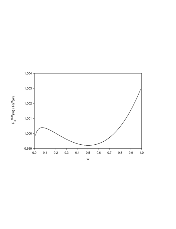
Figure 1: The ratio of the Padé prediction $R_{3}^{pade}(w)$ (27), and the $\chi^{2}$-minimizing fitted form $R_{3}^{fit}(w)$ (28c) as a function of $w$.

The $m_{A}=100\;GeV$ estimate for $c_{0}$ can be improved somewhat by using the correct values (24) of $c_{1-3}$ within equation (30), the lowest moment integral estimated in (34) by asymptotic Padé-approximant methods. We then find that

$$c_{0}=3310.4-1411-2(438.4)-6(28.16)=854.$$

Identically the same result is obtained by minimizing $\chi^{2}$ with respect to $c_{0}$ after explicit incorporation of the correct (RG) values (24) of $c_{1-3}$ into (36). There is a 15% discrepancy between (38) and the estimates for $c_{0}$ in (35) and (37), indicative of the magnitude of anticipated relative error with respect to the true value for $c_{0}$. It is hoped that these estimates can be tested against an exact 4-loop calculation in the not-too-distant future.

The 4-loop correction to the CP-odd Higgs decay into two gluons, as determined to 3-loop order in [1], is found from (1), (8) and (38):

$$\Gamma(A\rightarrow gg)=\frac{\sqrt{2}G_{F}m_{A}^{3}}{32\pi}\left[1+a_{0}x(m_{A})+b_{0}x^{2}(m_{A})+c_{0}x^{3}(m_{A})\right].$$

Given $n=5$, $m_{A}=100\;GeV$, $\alpha^{(5)}(m_{A})=0.116$ [1], and $m_{t}=175.6\;GeV$, the square bracketed expression in (39) for successive-loop corrections is $[1+0.680+0.226+{\underline{0.043}}]$. The first three numbers are as calculated in ref. [1]; the final (underlined) term is obtained from the asymptotic Padé-approximant estimate for $c_{0}$ in (38). This estimate is further indicative of a progressive decrease in the ratio of successive terms in the $A\rightarrow 2g$ decay rate, suggesting that if such a CP-odd Higgs were discovered, a perturbative calculation of its 2-gluon decay rate could lead to a phenomenologically testable value [e.g. 1 + 0.680 + 0.226 + 0.043 + … $\approx$ 2.0 for $m_{A}$ = 100 GeV]. Such a Higgs characterizes the two-doublet version of electroweak symmetry breaking anticipated from supersymmetric extensions of the standard model, as first noted over two decades ago [7].

Acknowledgment Support from the Natural Sciences and Engineering Research Council of Canada is gratefully acknowledged.

References

• [1] Chetyrkin K G, Kniehl B A, Steinhauser M, and Bardeen W A, 1998 Nucl. Phys. B 535 3
• [2] Chetyrkin K G, 1997 Phys. Lett. B 404 161; Larin S A, van Ritbergen T, Vermaseren J A M, 1997 Phys. Lett. B 405 327
• [3] Caso C et al [Particle Data Group], 1998 Eur. Phys. J. C 3 1; see also van Ritbergen T, Vermaseren J A M, and Larin, S A, 1997 Phys. Lett. B 400 379
• [4] Chishtie F, Elias V, and Steele, T G, 1999 Phys. Rev. D 59 105013
• [5] Ellis J, Jack I, Jones D R T, Karliner M, and Samuel M A, 1998 Phys. Rev. D 57 2665
• [6] Elias V, Steele T G, Chishtie F, Migneron R, and Sprague K, 1998 Phys. Rev. D 58 116007
• [7] Sherry T N, 1979 International Centre for Theoretical Physics Preprint IC/79/105