A Cosmology of the Brane World

Abstract

We develop a possible cosmology for a Universe in which there are $n$ additional spatial dimensions of variable scale, and an associated scalar field, the radion, which is distinct from the field responsible for inflation, the inflaton. Based on a particular ansatz for the effective potential for the inflaton and radion (which may emerge in string theory), we show that the early expansion of the Universe may proceed in three stages. During the earliest phase, the radion field becomes trapped at a value much smaller than the size of the extra dimensions today. Following this phase, the Universe expands exponentially, but with a Planck mass smaller than its present value. Because the Planck mass during inflation is small, we find that density fluctuations in agreement with observations can arise naturally. When inflation ends, the Universe reheats, and the radion becomes free to expand once more. During the third phase the Universe is “radiation-dominated” and tends toward a fixed-point evolutionary model in which the radius of the extra dimension grows, but the temperature remains unchanged. Ultimately, the radius of the extra dimensions becomes trapped once again at its present value, and a short period of exponential expansion, which we identify with the electroweak phase transition, ensues. Once this epoch is over, the Universe reheats to a temperature $\mathbin{\lower 3.0pt\hbox{$\hbox to0.0pt{\raise 5.0pt\hbox{$\char 60\relax$}\hss}\mathchar 29208\relax$}}m_{EW}$, the electroweak scale, and the mature Universe evolves according to standard cosmological models. We show that the present day energy density in radions can be smaller than the closure density of the Universe if the second inflationary epoch lasts $\sim 8$ e-foldings or more; the present-day radion mass turns out to be small ($m_{\rm radion}\mathbin{\lower 3.0pt\hbox{$\hbox to0.0pt{\raise 5.0pt\hbox{$\char 60\relax$}\hss}\mathchar 29208\relax$}}$ eV, depending on parameters). We argue that although our model envisages considerable time evolution in the Planck mass, substantial spatial fluctuations in Newton’s constant are not produced.

I Introduction

Recently it was suggested that the fundamental scale of gravity may be as low as TeV [1]. According to this idea, the observed weakness of gravity is associated with $n$ new, relatively large spatial dimensions (compactified to a size $\sim r_{0}$) in which only gravity can propagate. In this picture, all the standard model particles live in a set of branes with three extended space dimensions (“brane modes”), while gravitons live in the higher dimensional bulk of spacetime (“bulk modes”). This scenario turns out to be quite natural in (Type I) string theory. In this ”brane world” picture [2, 3], the standard model particles are open strings whose ends must end on the branes (e.g., stretched between branes), while gravitons are closed string states that can move away from the branes and into the bulk. The relation between today’s Planck scale $M_{\rm Pl}=1.2$ x $10^{19}$ GeV and the fundamental string scale $m_{s}$ is approximately given by

$$M_{\rm Pl}^{2}\sim m_{s}^{n+2}r_{0}^{n}$$ (1)

Phenomenological and astrophysical constraints imply that $m_{s}$ may be as low as a few TeV, with $n\geq 2$ [1, 4]. In string/M theory, $n\leq 7$, and in the brane world, $n=2$ is a reasonable choice [3]. In any case, $r_{0}$ must be fine-tuned to a very large value $m_{s}r_{0}\sim(M_{pl}/m_{s})^{2/n}\gg 1$; this fine-tuning problem is known as the radion problem. In this paper, we shall simply assume that the radius at $r_{0}$ is a stable minimum. However, as we shall see, this is not the end of the radion problem. One must still find a way for the radius to get to its final value without violating cosmological bounds. Some of the cosmological issues in the brane world have been discussed already [5, 6, 7, 8, 9, 10].

The main concern of the present paper is the cosmology in this framework, during the epoch before big bang nucleosynthesis, especially inflation [11]. Obviously, in the brane world, the standard cosmological picture is altered dramatically. In this paper, we present a plausible cosmological scenario where a number of issues in the brane world, such as inflation, density perturbation, reheating, baryogenesis, as well as the radion problem, are addressed. Our scenario incorporates the brane inflation feature [7] and some of its extensions [8], as well as some features of the rapid asymmetric inflation [9]. The main goal here is to show that cosmology in the brane world is viable, and highlight some of the issues that we believe to be important.

The reader may view this scenario as a search for viable potentials for the inflaton and the radion. The particular form we use has an effective potential for the radion field $r$ and inflaton fields ${\mbox{\boldmath$\psi$}}=(\psi_{1},\ldots,\psi_{N})$ such that

$$V({\mbox{\boldmath$\psi$}},r)=V_{0}({\mbox{\boldmath$\psi$}})[1+f_{\rm I}(r)]+f_{0}(r)+V_{1}({\mbox{\boldmath$\psi$}})$$ (2)

in the Jordan frame. (Appendix A gives some stringy justification for such a potential.) Here $V_{0}({\mbox{\boldmath$\psi$}})\sim m_{s}^{4}$ while $V_{1}({\mbox{\boldmath$\psi$}})\sim m_{\rm EW}^{4}\ll V_{0}$, where $m_{\rm EW}$ is the electroweak scale. Also the function $f_{\rm I}(r)$ tends to force the radion to some value $r_{\rm I}$ when $V_{0}({\mbox{\boldmath$\psi$}})$ is large, whereas $f_{0}(r)$ is unimportant until $r\to r_{0}$, where $r_{0}$ is the value of $r$ today. Instead of choosing $r_{0}$ to be the only minimum of $f_{0}(r)$, we choose $f_{0}(r)$ to have multiple minima, with $r_{0}$ just one of many possible minima. Our scenario utilizes an inflaton potential $V_{0}({\mbox{\boldmath$\psi$}})$ due to brane separation (see Appendix B), and incorporates a radion potential $f_{0}(r)$ (and $f_{\rm I}(r)$ as well) with multiple minima. To simplify the problem, we might assume that $V_{0}({\mbox{\boldmath$\psi$}})$ depends only on one component of $\psi$ and $V_{1}({\mbox{\boldmath$\psi$}})$ on the others (perhaps only one other); or, $\psi$ might only have one component with $V_{0}$ and $V_{1}$ both depending on this one component. The specific choices we examine for these potentials and functions are given in Eq. (33) for $V_{0}({\mbox{\boldmath$\psi$}})$, Eq. (D1) for $f_{I}(r)$, and Eqs. (75), (77) and (89) for $f_{0}(r)$. Here is a brief chronological description of the various phases of the scenario.

Phase 0: The pre-inflationary phase: The key feature of this phase is that the radion field $r$ is driven to a value $r_{I}$ at which it becomes fixed, thus allowing the subsequent stage of standard inflation to take place. The piece of the potential (2) that achieves this trapping is the term $V_{0}({\mbox{\boldmath$\psi$}})f_{I}(r)$; $r_{I}$ will be a local minimum of $f_{I}(r)$. The initial conditions for this phase that we assume are that the radii of the extra dimensions begin at values “around” $1/m_{s}$, where $m_{s}$ is the string scale (say, around 10 TeV). [By “around” we mean that values $\sim 1-100$ times larger than $m_{s}^{-1}$ are not out of the question.] Such initial conditions are natural since in string theory, the only scale is the string scale, and thus all parameters should typically scale like $m_{s}$ unless there are good reasons (such as dynamical evolution) for other values. In §II B we explore conditions under which the radion potential $f_{\rm I}(r)$ achieves the fixing of the radion to some value $r_{\rm I}$. A specific choice of functional form of $f_{I}(r)$, which may or may not correspond to reality, is discussed further in Appendix D. Generally speaking, we think it likely that if $f_{I}(r)$ has numerous potential minima separated by some scale $\sim m^{-1}$, then the radion will become trapped at a minimum at fairly large $mr$ (i.e. $mr\mathbin{\lower 3.0pt\hbox{$\hbox to0.0pt{\raise 5.0pt\hbox{$\char 62\relax$}\hss}\mathchar 29208\relax$}}$ a few), and that, if the radion settles to a potential minimum, it does so right away, without moving away from the potential well it starts in. The reason is that it is the Einstein-frame radion potential $\propto r^{-2n}f_{I}(r)$ that is relevant to the dynamics, not the Jordan-frame potential $\propto f_{I}(r)$ [see Eqs. (C15) and (14) below, and Appendix C for a discussion of the Jordan and Einstein frames]. It is plausible that $f_{I}(r)$ might have fixed amplitude of variation, so that the Einstein-frame potential will decrease $\propto r^{-2n}$ at large $r$. Even under these assumptions about $f_{\rm I}(r)$, the dual conditions that $r_{\rm I}$ should be “around” $m_{s}^{-1}$ and that $mr_{\rm I}\mathbin{\lower 3.0pt\hbox{$\hbox to0.0pt{\raise 5.0pt\hbox{$\char 62\relax$}\hss}\mathchar 29208\relax$}}$ (a few), can be satisfied for values of $m$ “around” $m_{s}$. If $f_{\rm I}(r)$ increases in amplitude at large $r$ rapidly enough to overcome the factor $r^{-2n}$, then it is possible that $r$ actually increases somewhat from its original value during this pre-inflation era before settling into a minimum at $r_{\rm I}$.

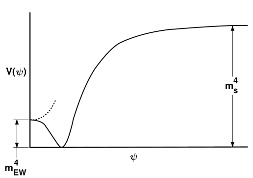
Phase I: Inflation at small Planck mass: Once the radion is fixed at the value $r_{I}$, slow-roll inflation can take place. The value of the Planck mass during inflation $M_{\rm Pl,I}$ is much smaller than today’s Planck mass $M_{\rm Pl}$, as $M_{\rm Pl,I}^{2}=(r_{I}/r_{0})^{n}M_{\rm Pl}^{2}$, where $r_{0}$ is the value of $r$ today. In the brane world, brane inflation [7] is quite natural. (A brief review is given in Appendix B.) In the brane inflation scenario, when branes are separated by a distance $d$, an effective potential $V(d)$ is generated by gravitational and other closed string exchanges between the branes. The distance $d$ plays the role of the inflaton. On the other hand, $d$ is related to the vacuum expectation value of a brane mode $\psi=m_{s}^{2}d$, so $V(\psi)$ is a function of a brane mode. In a particularly intriguing scenario, the electroweak Higgs field in the standard model plays the role of the inflaton $\psi$. In the $n=2$ case, the inflaton potential (schematically shown in Fig. 1), may be taken to have the following (oversimplified) qualitative form

$$V_{0}(\psi)+V_{1}(\psi)\sim m_{s}^{4}(1-e^{-|\psi|/m_{I}})+V_{1}(\psi)$$ (3)

with its minimum at $\psi\sim m_{EW}\sim$100 GeV.

FIG. 1.: The inflaton effective potential (not drawn to scale). The dashed line indicates the finite temperature effective potential after phase I.

For large $d$ (but still much smaller than $r_{I}$), $V\sim m_{s}^{4}$ is very flat, so the inflaton slowly rolls down the potential towards small $d$. In standard cosmology, the number of e-foldings required to solve the flatness and the horizon problems is around 60, but for brane cosmology, the required number of e-foldings is different [see Eqs. (111) and (126)], partly because the energy scale of inflation is $m_{s}\ll m_{GUT}\sim 10^{12}$TeV, but also because the Planck mass $M_{\rm Pl,I}$ during inflation is considerably smaller than today. [Fortuitously, the number of e-foldings required to solve the horizon and flatness problems may turn out to be about 60, see Eq. (126).]

The amplitude of primordial density perturbations generated by quantum fluctuations in the inflaton field during this inflationary epoch is $\sim m_{s}^{2}/m_{I}M_{\rm Pl,I}$ for the inflaton potential, Eq. (3). [See Eq. (44) in §II B.] Since $M_{\rm Pl,I}\sim m_{s}(m_{s}r_{\rm I})^{n/2}$, this amplitude is approximately $\sim m_{s}/m_{I}(m_{s}r_{\rm I})^{n/2}$, and to achieve the measured amplitude $\sim 10^{-5}$ of primordial perturbations [12], we must require $(m_{s}r_{I})^{n/2}\sim 10^{5}m_{s}/m_{I}$. For $m_{I}\sim m_{s}$, this would mean that $m_{s}r_{I}\gg 1$ (e.g. $\sim 10^{5}$ for $n=2$), but larger $m_{I}$ is expected naively (see Appendix B), and it is conceivable that $m_{s}r_{\rm I}\sim 1-100$ (i.e. larger than one but not by a factor as large as $10^{5}$).

Phase II: Radion growth and radiation domination: At the end of inflation, we expect the brane to be heated (since the inflaton $\psi$ is a brane mode) while the bulk remains relatively cold. We expect the reheat temperature $T_{r}$ to be below the Hagedorn temperature, which is typically lower than $m_{s}$ (say by a factor of 3 to 10). Since $m_{s}>>m_{EW}$, this temperature $T_{r}$ should be above the electroweak phase transition critical temperature $T_{{\rm c},1}$. So the finite temperature effective potential $V(\psi,T_{r})$ has a minimum at the origin, as indicated by the dashed line in Fig. 1. The inflaton rolls past the minimum of the $T=0$ potential towards $\psi=0$ and is trapped there. The rate of cooling to the bulk ($\sim T^{n+7}/m_{s}^{n+2}$) is very small, since $T/m_{s}$ is small. In this radiation dominated phase, the radion potential is negligible (which is not hard to arrange), while the inflaton field remains frozen. Under these conditions, we find that the cosmological model tends toward a fixed point in which the temperature remains nearly constant, while the radius $r$ grows as a power of time [see Eqs. (61) and (62)]. While this powerlaw solution holds, the radion potential energy is unimportant compared with its kinetic energy, which, however, decreases with time (and hence with increasing radius).

After sufficient time elapses, the kinetic energy of the radion field drops to a value comparable with the amplitude of the radion potential $f_{0}(r)$, and the growth of the radion, which is substantial up to this point, is halted. If $f_{0}(r)$ had only a single minimum, it would be a fantastic coincidence if (a) that minimum were precisely at the value $r_{0}$ and (b) the powerlaw growth of $r$ halted exactly when that minimum was encountered. Since powerlaw growth of $r$ during the radiation dominated phase that follows inflation is generic in our picture, it seems that we must require that the radion effective potential $f_{0}(r)$ have multiple minima. Since it is inevitable that the radion kinetic energy becomes smaller than the height of its effective potential after some elapsed time, the radion must become trapped at one of the minima of $f_{0}(r)$ eventually. As an illustration, we consider a periodic radion potential; $r_{0}$ is just one of the infinity of minima of this potential. That the Universe settles to $r_{0}$ is a cosmological accident in our scenario, although it is natural for the radion to settle to some radius much larger than its value during inflation (and much larger than the string scale $m_{s}^{-1}$). Thus, the radion problem is not so severe in our picture, which accommodates growth of the radius of the extra dimensions to a large, but stable value very simply. What we do not explain is why $r_{0}$ (and hence Newton’s constant) has a particular value among the infinity of possibilities. However, we identify what conditions must be satisfied by the underlying physical theory for the Universe to settle at $r_{0}$ [see Eqs. (82) and (83)].

Phase III: Second inflationary era and electroweak phase transition: When $T$ drops below $T_{{\rm c},1}$, the stable minimum of the inflaton will yield the spontaneous symmetry breaking of the electroweak model. It is reasonable to suppose that the electroweak phase transition is first-order. (This should be easy to arrange in models with multi-Higgs fields, e.g., the minimal supersymmetric standard model.) In this case, some super-cooling is expected and the actual phase transition happens during a period some time after $T$ has dropped below $T_{{\rm c},1}$. In the mean time, we expect considerable dilution of the radion energy density as well as the bulk energy density. Indeed, we show that requiring the radion density at present not to exceed the critical density for a flat Universe constrains the number of e-foldings of this inflationary era [see Eqs. (113) and (125)]. [Associated with the radion density today would be small-amplitude oscillations of Newton’s constant at a high frequency [13], [14]; see Eqs. (98) and §V.] This can be achieved by a short period of inflation during the super-cooling period, followed by either prompt or delayed reheating. The actual electroweak phase transition then takes place with the presence of nucleation bubbles. This allows the electroweak phase transition to complete and baryogenesis during this period can happen more or less as in the standard scenario [15]. Alternatively, baryogenesis can happen via the Affleck-Dine mechanism or some other mechanism [16]. In fact, it may take place before the end of the second inflationary era.

The final reheat temperature can be around a few GeV, maybe even close to the electroweak scale $m_{EW}$, if $m_{s}$ is large enough, and still avoid excessive cooling to the bulk, which would overproduce Kaluza-Klein (KK) modes, whose energy density could overclose the Universe and ruin the success of Big Bang nucleosynthesis. It is also high enough to provide the ”initial conditions” of the hot Big Bang before Big Bang nucleosynthesis.

The scenario is summarized in Fig. 2.

The basic plan of this paper is the following. In §II, we present our cosmological scenario; §II A gives some useful background (some of which is also found in Appendix C), §II B treats the pre-inflationary phase, §II C treats inflation at small Planck mass, and §II D treats the phase during which the radius of the extra dimensions grows from $r_{\rm I}$ to $r_{0}$. Some constraints on our model are gathered in §III. Density fluctuations during the epoch when the radion grows are discussed briefly in §IV. The results are discussed in §V. Some additional details about our cosmological model are contained in various Appendices.

II Matching Phases

A Setup

The starting point for our analysis is the following low energy action, which is valid when the lengthscales over which all fields vary are much larger than the size of the extra dimensions:

$$S = \int d^{4}x\sqrt{-{\hat{g}}}\bigg{[}{{\hat{R}}\over 16\pi G}-{1\over 2}({\hat{\nabla}}\Phi)^{2}-{1\over 2}e^{-\Phi/\mu}({\hat{\nabla}}{\mbox{\boldmath$\psi$}})^{2}-e^{-2\Phi/\mu}\,V({\mbox{\boldmath$\psi$}},\Phi)\bigg{]}$$ (5)

$$+S_{\rm rest}[e^{-\Phi/\mu}{\hat{g}}_{\alpha\beta},\chi_{\rm rest}].$$

This action is derived from the higher dimensional description in Appendix C. The action is written in the Einstein frame, ${\hat{g}}_{\alpha\beta}$ is the Einstein frame metric, and

$$g_{\alpha\beta}=e^{-\Phi/\mu}{\hat{g}}_{\alpha\beta}$$ (6)

is the physical, Jordan frame metric. The quantity $G$ is the usual 3-dimensional Newton’s constant, and $\mu$ is a mass of order the Planck mass $M_{\rm Pl}=\sqrt{c\hbar/G}=1.22\times 10^{19}\,{\rm GeV}$ given by

$$\mu=M_{\rm Pl}\,\sqrt{{n+2\over 32\pi n}},$$ (7)

where $n$ is the number of extra dimensions. The field $\Phi$ is the canonically normalized radion field, related to the radius $r$ of the extra dimensions by

$$r=r_{0}\exp\left[{\Phi\over n\mu}\right],$$ (8)

where $r_{0}$ is the equilibrium radius of the extra dimensions today. The fields ${\mbox{\boldmath$\psi$}}=(\psi_{1},\ldots,\psi_{N})$ are inflaton fields. The quantity $V({\mbox{\boldmath$\psi$}},\Phi)$ is the Jordan-frame potential for the radion and inflaton discussed in the Introduction and in Appendix A below. Finally the action $S_{\rm rest}[g_{\alpha\beta},\chi_{\rm rest}]$ is the action of the remaining matter fields $\chi_{\rm rest}$, which in our analysis below we will treat as a fluid.

As discussed above, we assume that the Jordan-frame effective potential $V({\mbox{\boldmath$\psi$}},\Phi)=V({\mbox{\boldmath$\psi$}},r)$ is of the form [cf. Eq. (2)]

$$V({\mbox{\boldmath$\psi$}},r)=V_{0}({\mbox{\boldmath$\psi$}})[1+f_{\rm I}(r)]+f_{0}(r)+V_{1}({\mbox{\boldmath$\psi$}}).$$ (9)

Here we might assume that $V_{0}$ depends only on one component of $\psi$ and $V_{1}$ on the other components (perhaps only one other). The function $f_{\rm I}(r)$ tends to force the radion to some value $r_{\rm I}$ while $V_{0}$ is large, whereas $f_{0}(r)$ is unimportant until $r\to r_{0}$, its value today. Following Ref. [7], we assume that $V_{0}({\mbox{\boldmath$\psi$}})\to 0$ as ${\mbox{\boldmath$\psi$}}\to 0$ and that $V_{0}({\mbox{\boldmath$\psi$}})$ asymptotes to a constant value, $\hat{V}_{0}$, exponentially with some mass scale(s) $m_{\rm I}$. The potential $V_{1}({\mbox{\boldmath$\psi$}})$ is assumed to have a minimum at nonzero $\psi$, and a value $\hat{V}_{1}\equiv V_{1}(0)$ at ${\mbox{\boldmath$\psi$}}=0$ which satisfies $\hat{V}_{1}\ll\hat{V}_{0}$.

We will do all our calculations in the Einstein frame. Assuming zero spatial curvature, the metric of the cosmological background in the Jordan frame can be written in the form

$$ds^{2}=-dt^{2}+a^{2}(t)d{\bf x}{\mbox{\boldmath$\cdot$}}d{\bf x},$$ (10)

and the corresponding metric in the Einstein frame is

$$d\hat{s}^{2}=e^{\Phi/\mu}\left[-dt^{2}+a^{2}(t)d{\bf x}{\mbox{\boldmath$\cdot$}}d{\bf x}\right]=-d\hat{t}^{2}+\hat{a}^{2}(\hat{t})d{\bf x}{\mbox{\boldmath$\cdot$}}d{\bf x},$$ (11)

where

$$d\hat{t}=\exp(\Phi/2\mu)\ dt\qquad\qquad\hat{a}(\hat{t})=\exp(\Phi/2\mu)\ a(t).$$ (12)

It is important to keep the relations (12) in mind, since proper time is not the same in the Einstein and Jordan frames, nor is the scale factor. In terms of $r$, the scalings are

$$d\hat{t}=(r/r_{0})^{n/2}dt\qquad\qquad\hat{a}(\hat{t})=(r/r_{0})^{n/2}a(t).$$ (13)

Thus, as $r$ changes, the relative rates of advance of time and scale factor differ in the two frames.

We treat the last term in the action (5) as a fluid with Jordan-frame density $\rho$ and pressure $p$. Then, the cosmological equations of motion that follow from the action (5) follow from the general equations of motion given in Appendix C, and are given by

$${\hat{H}}^{2}={8\pi\over 3M_{\rm Pl}^{2}}\bigg{[}{1\over 2}{\Phi}^{\prime 2}+{1\over 2}e^{-\Phi/\mu}{\psi}^{\prime 2}+e^{-2\Phi/\mu}V(\psi,\Phi)+e^{-2\Phi/\mu}\rho\bigg{]},$$ (14)

$${\Phi}^{\prime\prime}+3{\hat{H}}{\Phi}^{\prime}+ {\partial\over\partial\Phi}\left[e^{-2\Phi/\mu}V(\psi,\Phi)\right]+{1\over 2\mu}e^{-\Phi/\mu}\psi^{\prime 2}={\rho-3p\over 2\mu}e^{-2\Phi/\mu},$$ (15)

$${\psi}^{\prime\prime}+{\psi}^{\prime}\left[3{\hat{H}}-{\Phi^{\prime}\over\mu}\right]+e^{-\Phi/\mu}{\partial\over\partial\psi}V(\psi,\Phi)=0.$$ (16)

and

$${\rho}^{\prime}+3(\rho+p)\left[{\hat{H}}-{1\over 2\mu}{\Phi}^{\prime}\right]=0.$$ (17)

In these equations primes denote derivatives with respect to Einstein-frame proper time ${\hat{t}}$ [Eq. (10) above], and ${\hat{H}}$ is the Einstein-frame Hubble parameter ${\hat{H}}={\hat{a}}^{\prime}/{\hat{a}}$.

In the next few subsections, we shall substitute the potential (2) into the evolution equations (14) – (17), and solve for approximate solutions in the four different phases of cosmological evolution discussed in the Introduction.

B Phase 0: Radion to Its First Equilibrium

During Phase 0, the radion evolves to some size $r_{\rm I}$ where it remains pinned during inflation (phase I). This pinning happens by some time $\hat{t}_{0}$ when the scale factor is $\hat{a}_{0}$. The end of phase 0 signals the onset of the first inflationary phase, phase I

To see how the pinning might come about, let us assume that we can neglect the terms $f_{0}(r)$ and $V_{1}({\mbox{\boldmath$\psi$}})$, and that there is no energy density except what is due to $\psi$ and the radion. Furthermore, let us assume that the kinetic energy of the inflaton is negligible, and that $V_{0}({\mbox{\boldmath$\psi$}})\approx\hat{V}_{0}$. Then the Friedmann equations (14) and (15) together with the potential (2) simplify to

$$\hat{H}^{2}={8\pi\over 3M_{\rm Pl}^{2}}\biggl{\{}\hat{V}_{0}\exp(-2\Phi/\mu)[1+f_{\rm I}(r)]+{1\over 2}(\Phi^{\prime})^{2}\biggr{\}}$$ (18)

$$\Phi^{\prime\prime}+3\hat{H}\Phi^{\prime}={2\hat{V}_{0}\exp(-2\Phi/\mu)\over\mu}\biggl{[}1+f_{\rm I}(r)-{r\over 2n}{df_{\rm I}(r)\over dr}\biggr{]}.$$ (19)

We can render these equations non-dimensional by letting

$$\zeta=\exp[2(\Phi-\Phi_{i})/\mu]$$ (20)

and defining a new time variable $\tau$ by

$$d\hat{\tau}=\biggl{(}{8\pi{\hat{V}}_{0}\over 3M_{\rm Pl}^{2}}\biggr{)}^{1/2}\exp(-\Phi_{i}/\mu)d\hat{t},$$ (21)

where $\Phi_{i}$ is the initial value of $\Phi$, at the beginning of Phase 0. In terms of these new variables, we find ($f^{\prime}=df/d\hat{\tau}$ in these equations)

$$\biggl{(}{y^{\prime}\over y}\biggr{)}^{2}={1+f_{\rm I}(r)\over\zeta}+{1\over 2\nu}\biggl{(}{\zeta^{\prime}\over\zeta}\biggr{)}^{2}$$ (22)

$$\zeta^{\prime\prime}+\biggl{(}{3y^{\prime}\over y}-{\zeta^{\prime}\over\zeta}\biggr{)}\zeta^{\prime}=\nu\biggl{[}1+f_{\rm I}(r)-{r\over 2n}{df_{\rm I}(r)\over dr}\biggr{]}.$$ (23)

Here $y=\hat{a}/\hat{a}_{i}$, with $\hat{a}_{i}$ the initial value of the Einstein frame scale factor, $r=r_{i}\zeta^{1/2n}$, with $r_{i}$ the initial value of the radius of the extra dimensions, and

$$\nu\equiv{48n\over n+2}.$$ (24)

It is easy to see that if $f_{\rm I}(r)=0$, the solution of Eq. (23) tends to

$$y\propto\hat{\tau}^{1/3}\qquad\zeta\propto\hat{\tau}^{\sqrt{2\nu}/3},$$ (25)

according to which $r$ grows without bound, and the radion kinetic energy dominates the energy density of the Universe, but there is no inflation [17]. The approach to this asymptotic solution may be very slow: for example, for $n=2$ we have $\zeta\propto\hat{\tau}^{4/\sqrt{3}}$, so the vacuum energy density declines $\propto\hat{\tau}^{4/\sqrt{3}}$, which is only a bit faster than the rate of decline of the radion kinetic energy, $1/\hat{\tau}^{2}$. Nevertheless, it is noteworthy that without the radion potential, $r$ would grow to infinity in this phase.

To halt the growth of $r$, the radion potential must be capable of trapping the radion field. From Eq. (23), we see that this is only possible if the condition

$$1+f_{\rm I}(r)-{r\over 2n}{df_{\rm I}(r)\over dr}=0$$ (26)

can be satisfied. If we consider the choice $f_{I}(r)=(mr)^{\kappa}$ for example, where $m$ is a mass parameter and $\kappa>0$, then it is clear that Eq. (26) will only have real solutions for $\kappa>2n$ in which case the radion could settle to a value $mr=(\kappa/2n-1)^{-1}$. (Analogously shifted minima have been discussed by e.g. Steinhardt & Will [14].) However, such steeply growing functions $f(r)$ could prevent $r$ from growing to a large value later on.

Instead, we shall consider the possibility that

$$f_{\rm I}(r)=aF(r),$$ (27)

where $a$ is a dimensionless amplitude factor, and $F(r)$ has multiple minima, separated by a characteristic scale $\sim m^{-1}$, with “potential barriers” $|F(r)|\sim 1$. A specific example (but not unique or required) is $F(r)=1-\cos mr$, for which Eq. (26) becomes

$$1+a(1-\cos mr)-{amr\sin mr\over 2n}=0.$$ (28)

Since $\cos mr\leq 1$ and $\sin mr\leq 1$, there are no solutions to this equation unless $amr/2n>1$, or $mr>2n/a$. Thus, unless $a$ is large (which we consider unlikely), the radion will only settle into minima at relatively large values of $mr$, if at all. This conclusion ought to hold for other choices of $F(r)$ with similar qualitative properties. If, for example, $m\sim m_{s}$, then we conclude that the radion will only settle on values larger than the string scale, which, in fact, is required for consistency of our entire picture. (Remember that, for example, $r$ must exceed the brane separation.)

For $f_{\rm I}(r)$ of this general type, it seems likely that the radion must settle into its first minimum, the one nearest its value at the onset of Phase 0, if it settles to a minimum at all. The reason is that the height of the Einstein frame effective potential decreases with increasing $r$, so that if the radion acquires sufficient kinetic energy to roll over the first barrier it encounters, it should be able to overcome all subsequent barriers. (Remember that in the asymptotic solutions to Eq. [23] the energy density of the Universe becomes dominated by radion kinetic energy as time progresses.) We explore the particular example $F(r)=1-\cos mr$ in some detail in Appendix D. It is also important to note, though, that it is possible to imagine choices for $f_{\rm I}(r)$ that undo the decrease factor in amplitude $\propto r^{-2n}$ in Eq. (19) at large $r$. For such potentials, it might be possible for $r$ to evolve considerably before settling to a potential minimum.

C Phase I: Inflation at Small Planck Mass

During Phase I, the Universe inflates at a fixed radion radius, $r_{\rm I}$. This fixes the Planck mass to be

$$M_{\rm Pl,I}^{2}=(r_{\rm I}/r_{0})^{n}M_{\rm Pl}^{2},$$ (29)

and the expansion rate is

$$\hat{H}_{I}^{2}=\biggl{(}{\hat{a}^{\prime}\over\hat{a}}\biggr{)}^{2}={8\pi r_{0}^{2n}\hat{V}_{0}\over 3M_{\rm Pl}^{2}r_{\rm I}^{2n}}={8\pi r_{0}^{n}\hat{V}_{0}\over 3M_{\rm Pl,I}^{2}r_{\rm I}^{n}}$$ (30)

in the Einstein frame, where prime denotes differentiation with respect to $\hat{t}$. The Jordan frame expansion rate is simply

$$H_{I}^{2}=\biggl{(}{\dot{a}\over a}\biggr{)}^{2}={8\pi\hat{V}_{0}\over 3M_{\rm Pl,I}^{2}},$$ (31)

where dot denotes differentiation with respect to $t$; this is just as in the usual general relativity but with a different Planck mass. The scale factor in this phase is

$${\hat{a}\over\hat{a}_{0}}=\exp[\hat{H}_{I}(\hat{t}-\hat{t}_{0})]={a\over a_{0}}=\exp[H_{I}(t-t_{0})].$$ (32)

Since the radius of the extra dimensions is frozen in phase I, it is equally easy to use the Jordan or Einstein frame descriptions. (The same will not be true for subsequent phases.)

Presuming that a single inflaton field is important in this phase, with an effective potential

$$V_{0}(\psi)=\hat{V}_{0}[1-\exp(-\psi/m_{\rm I})],$$ (33)

the inflaton equation of motion is

$$\ddot{\psi}+3H_{I}\dot{\psi}=-{\hat{V}_{0}\over m_{\rm I}}\exp(-\psi/m_{\rm I}).$$ (34)

The evolution of the inflaton proceeds in two subphases. During the first subphase, we have the usual slow-rolling approximation,

$$\dot{\psi}\approx-{\hat{V}_{0}\exp(-\psi/m_{\rm I})\over 3H_{I}m_{\rm I}},$$ (35)

whose solution is

$$\exp(\psi/m_{\rm I})=\exp(\psi_{0}/m_{\rm I})-{\hat{V}_{0}(t-t_{0})\over 3m_{\rm I}^{2}H_{I}}=\exp(\psi_{0}/m_{\rm I})-{M_{\rm Pl,I}^{2}\over 8\pi m_{\rm I}^{2}}H_{I}(t-t_{0}).$$ (36)

This approximate solution holds as long as the two conditions

$$\biggl{|}{\ddot{\psi}\over 3H_{I}\dot{\psi}}\biggr{|}\approx{M_{\rm Pl,I}^{2}\exp(-\psi/m_{\rm I})\over 24\pi m_{\rm I}^{2}}\ll 1\qquad\qquad{\dot{\psi}^{2}\over 2\hat{V}_{0}}\approx{M_{\rm Pl,I}^{2}\exp(-2\psi/m_{\rm I})\over 48\pi m_{\rm I}^{2}}\ll 1$$ (37)

are satisfied. Assuming that $M_{\rm Pl,I}\gg m_{\rm I}$, which emerges naturally later, the first of these two conditions fails first, when

$$\exp(\psi/m_{\rm I})\sim{M_{\rm Pl,I}^{2}\over 24\pi m_{\rm I}^{2}}.$$ (38)

If the initial value $\exp(\psi_{0}/m_{\rm I})$ of $\exp(\psi/m_{\rm I})$ is far larger than the limit (38), then the time required for the inflaton field to reach this magnitude is extremely large, given by

$$H_{I}(t_{\rm sr}-t_{0})\approx{8\pi m_{\rm I}^{2}\over M_{\rm Pl,I}^{2}}\exp(\psi_{0}/m_{\rm I}),$$ (39)

where $t_{\rm sr}$ is the time at the end of slow-roll, which implies many e-foldings during inflation. When slow-rolling ends, a second sub-phase of inflaton evolution begins. Since the kinetic energy of the inflaton at the beginning of this subphase is only $\sim(12\pi m_{\rm I}^{2}/M_{\rm Pl,I}^{2})\hat{V}_{0}\ll\hat{V}_{0}$, the inflaton moves on approximately a “zero energy solution with negligible damping”. That is, it satisfies the equation

$$\dot{\psi}\approx-\sqrt{2\hat{V}_{0}}\exp(-\psi/2m_{\rm I}),$$ (40)

which has the solution

$$\exp(\psi/2m_{\rm I})=\exp(\psi_{sr}/2m_{\rm I})-\sqrt{\hat{V}_{0}\over 2m_{\rm I}^{2}}(t-t_{\rm sr})=\exp(\psi_{sr}/2m_{\rm I})-\sqrt{3\over 16\pi}{M_{\rm Pl,I}\over m_{\rm I}}H_{I}(t-t_{\rm sr}),$$ (41)

where $\exp(\psi_{sr}/2m_{\rm I})\sim M_{\rm Pl,I}/m_{\rm I}\sqrt{24\pi}$. The time remaining for $\psi\to 0$ is not large: $H_{I}(t_{\rm end}-t_{\rm sr})\sim 1$, where $t_{\rm end}$ signifies the end of this inflationary epoch, and henceforth we do not distinguish between the two times $t_{\rm sr}$ and $t_{\rm end}$.

Using our approximate expression for $H_{I}(t_{\rm sr}-t_{0})\approx H_{I}(t_{\rm end}-t_{0})$, we rewrite the slow rolling solution as

$$\exp(\psi/m_{\rm I})\approx{M_{\rm Pl,I}^{2}\over 8\pi m_{\rm I}^{2}}H_{I}(t_{\rm end}-t).$$ (42)

From this and the slow rolling approximation it follows that

$$\dot{\psi}\approx-{m_{\rm I}\over t_{\rm end}-t}.$$ (43)

The primordial density perturbation amplitude is then [18]

$${\delta\rho\over\rho}\sim{H_{I}^{2}\over\dot{\psi}}\approx{\sqrt{8\pi\hat{V}_{0}/3}\over m_{\rm I}M_{\rm Pl,I}}N_{k},$$ (44)

where $N_{k}$ is the number of e-foldings that remain between horizon crossing for a scale of comoving length $\sim k^{-1}$ and the end of Phase I. We note that the spectrum of inhomogeneities implied by Eq. (44) is insensitive to $k$, in agreement with observations [12]. If the effective potential as a function of interbrane separation $d$ is proportional to $1-\exp(-m_{d}d)$, and we set $\psi=m_{s}^{2}d$, then $m_{d}d=m_{d}\psi/m_{s}^{2}$, which implies $m_{\rm I}=m_{s}^{2}/m_{d}$. Then the amplitude of the density fluctuations is proportional to $\sqrt{\hat{V}_{0}}m_{d}/m_{s}^{2}M_{\rm Pl,I}$, which, for $\hat{V}_{0}\sim m_{s}^{4}$, is $\sim m_{d}/M_{\rm Pl,I}$. Note also that since the radion is trapped, fluctuations in $r$ are suppressed [see Eq. (D9) of Appendix D].

D Phase II: Radiation Domination

At the end of inflation, $\hat{t}=\hat{t}_{1}$ and $\hat{a}=\hat{a}_{1}$; the Universe reheats to a temperature $\epsilon\hat{V}_{0}^{1/4}$ where $\epsilon<1$ depends on how efficiently the kinetic energy of the inflaton is thermalized once ${\mbox{\boldmath$\psi$}}\to 0$.

Reheating will alter the effective potential so that there is a minimum at ${\mbox{\boldmath$\psi$}}=0$, provided that the critical temperature $T_{{\rm c},1}$ for the phase transition (presumed first order) connected with the potential $V_{1}({\mbox{\boldmath$\psi$}})$ is small compared with the reheating temperature. In this case, there will be a nonzero vacuum energy $\hat{V}_{1}$, but as long as the temperature remains above $T_{{\rm c},1}$, the Universe remains radiation-dominated, and $\psi$ is pinned at zero.

We assume that the radion potential becomes negligible when this happens. Let us explore the growth in the radion field that ensues.

It is most convenient to work in the Einstein frame. This phase of evolution will divide into three subphases. During the first subphase, when radiation dominates, the Friedmann equations are [cf. Eqs. (14) and (17) above with $p=\rho/3$]

$$\hat{H}^{2}={8\pi\over 3M_{\rm Pl}^{2}}\rho\exp(-2\Phi/\mu)\qquad\qquad\rho\hat{a}^{4}\exp(-2\Phi/\mu)={\rm constant},$$ (45)

where we recall that $\rho$ is the Jordan frame energy density i.e. $\rho\sim T^{4}$. Thus, the scale factor in Einstein frame is simply

$$\hat{a}=\hat{a}_{1}\biggl{(}{\hat{t}\over\hat{t}_{1}}\biggr{)}^{1/2},$$ (46)

just as it would be in constant-$M_{\rm Pl}$ cosmology. However, to find out how fast the temperature decreases, we also need to know how the radion field evolves.

Under the assumption that the radion potential is negligible, we find from Eqs. (2), (15) and (33) the evolution equation

$$\Phi^{\prime\prime}+3\hat{H}\Phi^{\prime}={2\hat{V}_{1}\over\mu}\exp(-2\Phi/\mu).$$ (47)

We make the change of variables

$$u=\exp(2\Phi/\mu).$$ (48)

Then Eq. (47) is equivalent to

$$u^{\prime\prime}+\biggl{(}{3\hat{H}}-{u^{\prime}\over u}\biggr{)}u^{\prime}=u^{\prime\prime}+\biggl{(}{3\over 2\hat{t}}-{u^{\prime}\over u}\biggr{)}u^{\prime}={4\hat{V}_{1}\over\mu^{2}},$$ (49)

where $\hat{H}=1/2\hat{t}$, appropriate for this subphase, has been used. During the first subphase,

$${3\over 2\hat{t}}\gg{u^{\prime}\over u}.$$ (50)

In that case, under the assumption that $u^{\prime}=0$ and $u=u_{1}$ at $\hat{t}=\hat{t}_{1}$, we find

$$u^{\prime}={8\hat{V}_{1}\over 5\mu^{2}}\biggl{(}\hat{t}-{\hat{t}_{1}^{5/2}\over\hat{t}^{3/2}}\biggr{)},$$ (51)

which can be integrated to yield

$$u=u_{1}+{4\hat{V}_{1}\over 5\mu^{2}}\biggl{(}\hat{t}^{2}-5\hat{t}_{1}^{2}+{4\hat{t}_{1}^{5/2}\over\hat{t}^{1/2}}\biggr{)}.$$ (52)

This solution holds as long as Eq. (50) is true, a condition that fails when

$${2\hat{t}u^{\prime}\over 3u}\approx{16\hat{V}_{1}\hat{t}^{2}/15\mu^{2}\over u_{1}+4\hat{V}_{1}\hat{t}^{2}/5\mu^{2}}\sim 1,$$ (53)

or

$$u_{1}\sim{\hat{V}_{1}\hat{t}^{2}\over\mu^{2}}.$$ (54)

(In getting this condition, we have assumed that the first subphase ends at a time $\gg\hat{t}_{1}$.) Since $u=\exp(2\Phi/\mu)$ is still only a factor of two or so different from $u_{1}$, it follows that

$$\rho={\rho_{1}\hat{a}_{1}^{4}\exp(2\Phi/\mu)\over\hat{a}^{4}\exp(2\Phi_{1}/\mu)}={\rho_{1}\hat{V}_{1}\hat{t}_{1}^{2}u\over\mu^{2}u_{1}^{2}}\sim{\rho_{1}\hat{V}_{1}\hat{t}_{1}^{2}\over\mu^{2}u_{1}},$$ (55)

where in the first equality we used Eqs. (46), (48) and (54). Using

$$t_{1}^{2}\sim{3M_{\rm Pl,I}^{2}\over 8\pi\rho_{1}}\sim{M_{\rm Pl}^{2}\sqrt{u_{1}}\over\rho_{1}},$$ (56)

and $\hat{t}_{1}^{2}=\sqrt{u_{1}}t_{1}^{2},$ we find

$$\rho\sim\hat{V}_{1}$$ (57)

since $\mu\sim M_{\rm Pl}$. Thus, the first subphase ends when the energy density in radiation becomes comparable to the vacuum energy in the inflaton. The value of the Planck mass only changes by a factor of order unity during this regime.

During the second subphase, the radion potential is still unimportant, but the radion kinetic energy is not. Thus, the radion evolves according to Eq. (49), but the expansion rate in the Einstein frame is given by

$$\hat{H}^{2}={8\pi\over 3M_{\rm Pl}^{2}}\biggl{[}{\rho\over u}+{V_{1}(\psi)\over u}+{\mu^{2}\over 8}\biggl{(}{u^{\prime}\over u}\biggr{)}^{2}+{(\psi^{\prime})^{2}\over 2\sqrt{u}}\biggr{]}.$$ (58)

The evolution of the inflaton field is governed by the equation

$$\psi^{\prime\prime}+3\hat{H}\psi^{\prime}=-u^{-1/2}{dV_{1}(\psi)\over d\psi}.$$ (59)

We assume that the Universe remains hot enough that the inflaton is trapped in a symmetric phase, at fixed fixed vacuum energy density $\hat{V}_{1}$ during this subphase. At least at first, the kinetic energy of the inflaton field will be unimportant, and we can approximate the expansion rate by

$$\hat{H}^{2}={8\pi\over 3M_{\rm Pl}^{2}}\biggl{[}{\rho\over u}+{\hat{V}_{1}\over u}+{\mu^{2}(u^{\prime})^{2}\over 8u^{2}}\biggr{]}.$$ (60)

It is easy to see that at the start of this subphase, the three contributions to the energy density are comparable to one another. Moreover, there is a simple, powerlaw solution to the fully nonlinear problem defined by eqs. (49) and (60). For this solution, $\hat{a}\propto\sqrt{\hat{t}}$, and

$$u={4\hat{V}_{1}\hat{t}^{2}\over\mu^{2}}\qquad{u^{\prime}\over u}={2\over\hat{t}};$$ (61)

since $\rho\hat{a}^{4}/u=$constant, $\rho=$constant. From Eq. (60) we find a consistency condition

$${\rho\over\hat{V}_{1}}={9n-6\over n+2},$$ (62)

which gives $\rho/\hat{V}_{1}=3$ for $n=2$, for example; thus, the temperature remains $\sim\hat{V}_{1}^{1/4}$, and could be comfortably above the critical temperature for the inflaton in this regime. Within this solution, it also follows that, up to a possible additive constant,

$$t={\sqrt{2\mu\hat{t}}\over\hat{V}_{1}^{1/4}},$$ (63)

and therefore, as a function of $t$, the radion expands according to

$$u={\hat{V}_{1}^{4}t^{4}\over\mu^{4}},$$ (64)

and grows without any expansion of the Universe at all in the Jordan frame.

It is worth investigating the meaning of this powerlaw solution further. Clearly, a solution in which the temperature remains constant is not expanding in the Jordan frame at all. Such a solution ought to apply only in a limiting sense. That is, the correct solution might approach this one asymptotically, at late times. To see if this happens, we consider the numerical solution eqs. (49) and (60), with the energy-conservation condition $\rho\hat{a}^{4}/u$=constant. We arbitrarily choose $u=u_{i}$ and $\rho=\rho_{i}$ at some initial time $\hat{t}_{i}$, when $\hat{a}\equiv\hat{a}_{i}$. If we define

$$y\equiv{\hat{a}\over\hat{a}_{i}}\qquad{\rm and}\qquad\zeta\equiv{u\over u_{i}},$$ (65)

and define a dimensionless Einstein-frame time variable by

$$d\hat{\tau}=(8\pi\rho_{i}/3M_{\rm Pl}^{2}u_{i})^{1/2}d\hat{t},$$ (66)

then we find the two coupled equations

$$\biggl{(}{y^{\prime}\over y}\biggr{)}^{2}={1\over 2\nu}\biggl{(}{\zeta^{\prime}\over\zeta}\biggr{)}^{2}+{v\over\zeta}+{1\over y^{4}}$$ (67)

$$\zeta^{\prime\prime}+\biggl{(}{3y^{\prime}\over y}-{\zeta^{\prime}\over\zeta}\biggr{)}\zeta^{\prime}=\nu v,$$ (68)

where

$$\nu\equiv{48n\over n+2}\qquad{\rm and}\qquad v\equiv{\hat{V}_{1}\over\rho_{i}}.$$ (69)

We can also evaluate the Jordan frame scale factor from

$$\hat{a}=u^{1/4}a,$$ (70)

and can find the time elapsed in the Jordan frame using

$$d\hat{t}=u^{1/4}dt,$$ (71)

which we rescale by defining $\tau_{J}=(8\pi\rho_{i}/3M_{\rm Pl}^{2}\sqrt{u_{i}})^{1/2}t$, to get $\tau_{J}^{\prime}=\zeta^{-1/4}$. Eqs. (68) are to be solved with initial conditions $\zeta=y=1$ at $\hat{\tau}=\hat{\tau}_{i}$; we can choose $\hat{t}_{i}$ arbitrarily (although we expect it to be $\approx 0.5$ if we want a solution that has $y\to 0$ at $\hat{\tau}\to 0$). The solutions depend only on the two parameters, $\nu$ and $v$; in terms of these, the powerlaw solution found previously becomes

$$\zeta=\nu v\hat{\tau}^{2}={48nv\hat{\tau}^{2}\over n+2}\qquad\qquad y=\biggl{(}{1\over 4}-{3\over\nu}\biggr{)}^{-1/4}\hat{\tau}^{1/2}=\biggl{(}{16n\over 3n-2}\biggr{)}^{1/4}\hat{\tau}^{1/2}$$ (72)

Numerical evaluations for $n=2$ show that, although the solutions oscillate slightly at late times, they approach the simple solution found above to high accuracy. From examining the output, it appears that the Jordan frame scale factor actually does not remain precisely constant at late times, but increases and even decreases slightly (by less than 10%) as time progresses.

In the asymptotic regime of the second subphase, the radion grows according to

$$u=(r/r_{0})^{2n}={4\hat{V}_{1}\hat{t}^{2}\over\mu^{2}},$$ (73)

so $u\to 1$, or $r\to r_{0}$, at a time

$$\hat{t}_{r\to r_{0}}={\mu\over 2\sqrt{\hat{V}_{1}}}$$ (74)

if this solution continues to hold. Note that $\hat{t}_{r\to r_{0}}\sim u_{1}^{-1/2}\hat{t}_{i}$, where $\hat{t}_{i}$ marks the onset of this subphase (or the end of the first subphase; e.g. Eq. [54]); since $u_{1}\ll 1$, $\hat{t}_{r\to r_{0}}\gg\hat{t}_{i}$.

In order for the radion to become pinned at $r=r_{0}$ we need a coincidence to happen: near the time $\hat{t}_{r\to r_{0}}$, the radion potential itself must begin to play a central role in the evolution of the field. Only the radion’s potential can make it settle into a minimum, rather than rolling forever to ever increasing radius. Indeed, what we want is for the effective potential of the radion to have many possible minima, so that the value it settles into eventually is determined by this coincidence.

To understand the settling process better, we need to incorporate the radion potential term $f_{0}(r)$ of the Jordan-frame potential (2) in out analyses. If $V_{\rm bulk}(r)$ is the radion potential in $4+n$ dimensions, then, after integrating over the $n$ extra dimensions, the corresponding Jordan frame potential is

$$f_{0}(r)=r^{n}V_{\rm bulk}(r)$$ (75)

[see Appendix C], and the Einstein frame potential $V_{E}$ obtained after conformal transformation is

$$V_{E}=r_{0}^{2n}r^{-n}V_{\rm bulk}(r)={r_{0}^{n}\exp(-\Phi/\mu)V_{\rm bulk}(r)}={r_{0}^{n}V_{\rm bulk}(r)\over\sqrt{u}}.$$ (76)

Suppose that

$$V_{\rm bulk}(r)=U_{\rm bulk}F(r),$$ (77)

where $U_{\rm bulk}$ is a constant and $F(r)$ is dimensionless. We assume that $F(r)$ may undulate up and down, but with a characteristic amplitude $|F(r)|\sim 1$; thus the scale of the radion potential is determined by $U_{\rm bulk}$. Since $F(r)$ is dimensionless, it must contain mass scales; these are reflected in the magnitude(s) of the derivative(s) of the potential. We assume that $F(r)$ may have multiple minima (an infinite number in the model considered below.)

One condition for the radion to be able to settle into one of the minima of its potential is that the Einstein frame kinetic energy density fall below the Einstein frame potential energy amplitude. Since the kinetic energy is

$${\mu^{2}\over 8}\biggl{(}{u^{\prime}\over u}\biggr{)}^{2}={\mu^{2}\over 2\hat{t}^{2}},$$ (78)

and the potential energy amplitude is

$${r_{0}^{n}U_{\rm bulk}\over\sqrt{u}}={r_{0}^{n}U_{\rm bulk}\mu\over 2\hat{t}\sqrt{\hat{V}_{1}}},$$ (79)

during the powerlaw regime, the two become comparable at at an Einstein frame time

$$\hat{t}={\mu\sqrt{\hat{V}_{1}}\over r_{0}^{n}U_{\rm bulk}}.$$ (80)

This time ought to be smaller than or comparable to the time at which $u\to 1$ i.e. we must require

$${\mu\sqrt{\hat{V}_{1}}\over r_{0}^{n}U_{\rm bulk}}\sim{\mu\over 2\sqrt{\hat{V}_{1}}},$$ (81)

which implies

$$r_{0}^{n}U_{\rm bulk}\sim 2\hat{V}_{1}.$$ (82)

Since, presumably, $U_{\rm bulk}$ and $\hat{V}_{1}$ are determined by fundamental physics, this relationship may be taken to determine $r_{0}^{n}$. Moreover, since we know that $M_{\rm Pl}^{2}\sim m_{s}^{2+n}r_{0}^{n}$, we find

$$M_{\rm Pl}^{2}\sim{2\hat{V}_{1}m_{s}^{2+n}\over U_{\rm bulk}}\qquad{\rm or}\qquad U_{\rm bulk}\sim{2\hat{V}_{1}m_{s}^{2+n}\over M_{\rm Pl}^{2}}.$$ (83)

If we assume that $\hat{V}_{1}\sim m_{EW}^{4}$, where $m_{EW}$ is the electroweak unification scale, and $m_{s}>m_{EW}$, then it is clear that $U_{\rm bulk}/m_{s}^{4+n}\sim{m_{EW}^{4}/M_{\rm Pl}^{2}m_{s}^{2}}\ll 1$. In getting these estimates, we have presumed that $F(r)$ takes on a typical value for $r\sim r_{0}$ i.e. we are excluding the possibility that, for example $|F(r\sim r_{0})|\ll 1$, which would alter the above estimates. This amounts to assuming that whatever the mass scales appear in $F(r)$ are generally of order $r_{0}^{-1}$ or larger.

To investigate the settling process in more detail, we need the equations of motion, which can be obtained from Eqs. (14) and (15). The resulting equations are

$$\hat{H}^{2}={8\pi\over 3M_{\rm Pl}^{2}}\biggl{[}{\rho\over u}+{\hat{V}_{1}\over u}+{\mu^{2}(u^{\prime})^{2}\over 8u^{2}}+{\Upsilon\hat{V}_{1}\over\sqrt{u}}F(r_{0}u^{1/2n})\biggr{]}$$ (84)

$$u^{\prime\prime}+\biggl{(}3\hat{H}-{u^{\prime}\over u}\biggr{)}{u^{\prime}\over u}={4\hat{V}_{1}\over\mu^{2}}-{2\Upsilon\hat{V}_{1}\sqrt{u}\over\mu^{2}}\biggl{[}{r\over n}{dF(r)\over dr}-F(r)\biggr{]}_{r=r_{0}u^{1/2n}}.$$ (85)

These equations are augmented by the conservation condition $\rho\hat{a}^{4}/u=$constant. Also we have defined

$$\Upsilon\equiv{r_{0}^{n}U_{\rm bulk}\over\hat{V}_{1}},$$ (86)

which we expect to be $\sim 2$. If we nondimensionalize as before we find

$$\biggl{(}{y^{\prime}\over y}\biggr{)}^{2}={1\over 2\nu}\biggl{(}{\zeta^{\prime}\over\zeta}\biggr{)}^{2}+{v\over\zeta}+{1\over y^{4}}+{v\Upsilon\sqrt{u_{i}}\over\zeta^{1/2}}F(r_{i}\zeta^{1/2n})\qquad\qquad\qquad$$ (87)

$$\zeta^{\prime\prime}+\biggl{(}{3y^{\prime}\over y}-{\zeta^{\prime}\over\zeta}\biggr{)}\zeta^{\prime}=\nu v-{\nu v\Upsilon\sqrt{u_{i}}\over 2}\zeta^{1/2}\biggl{[}{r\over n}{dF(r)\over dr}-F(r)\biggr{]}_{r=r_{i}\zeta^{1/2n}}.$$ (88)

Notice that in this form of the equations, $\Upsilon$ only appears in the combination $\Upsilon_{i}\equiv\Upsilon\sqrt{u_{i}}$, and since we expect $u_{i}\ll 1$, this parameter is small, implying that deviations from the powerlaw solution only appear at late times, as we have already concluded.

These equations contain three parameters explicitly: $n$ (or $\nu$), $v=\hat{V}_{1}/\rho_{i}$, and $\Upsilon_{i}$. In addition, they contain one (or more) parameters implicitly, because of the mass scales implicit in $F(r)$. For example, if

$$F(r)=1-\cos(m_{r}r),$$ (89)

so that there is only one mass scale, $m_{r}$, there is an additional nondimensional parameter $\mu_{i}\equiv m_{r}r_{i}$. For this form of $F(r)$, the evolution equations are

$$\biggl{(}{y^{\prime}\over y}\biggr{)}^{2}={1\over 2\nu}\biggl{(}{\zeta^{\prime}\over\zeta}\biggr{)}^{2}+{v\over\zeta}+{1\over y^{4}}+{v\Upsilon_{i}\over\zeta^{1/2}}[1-\cos(\mu_{i}\zeta^{1/2n}]\qquad\qquad\qquad$$ (90)

$$\zeta^{\prime\prime}+\biggl{(}{3y^{\prime}\over y}-{\zeta^{\prime}\over\zeta}\biggr{)}\zeta^{\prime}=\nu v-{\nu v\Upsilon_{i}\over 2}\zeta^{1/2}\biggl{[}{\mu_{i}\zeta^{1/2n}\sin(\mu_{i}\zeta^{1/2n})\over n}-1+\cos(\mu_{i}\zeta^{1/2n})\biggr{]}.$$ (91)

In these units, substantial deviations from the scaling equations are expected after

$$\hat{\tau}=\Upsilon_{i}^{-1}\sqrt{n+2\over 12nv},$$ (92)

at which time $\zeta=4/\Upsilon_{i}^{2}$, provided that $\mu_{i}\mathbin{\lower 3.0pt\hbox{$\hbox to0.0pt{\raise 5.0pt\hbox{$\char 62\relax$}\hss}\mathchar 29208\relax$}}(\Upsilon_{i}/2)^{1/n}$.

Fig. 2 shows the results of numerically integrating the dimensionless evolution equations, eqs. (91), for $(v,\Upsilon_{i},\mu_{i})=(10^{-6},10^{-8},10^{-3})$ (Fig. 2a) and $(v,\Upsilon_{i},\mu_{i})=(10^{-4},10^{-6},10^{-2})$ (Fig. 2b), respectively, with $n=2$ in both cases. The numerical results show clearly that after a long period of powerlaw expansion (in close agreement with the fixed point solution found above), $\zeta$ levels off, although in both cases, the time at which this happens is a bit later than our back-of-envelope estimate, so that $\zeta$ is systematically larger than $4/\Upsilon_{i}^{2}$ asymptotically. For $\Upsilon_{i}=10^{-6}$, we would estimate $\zeta=4\times 10^{12}$ asymptotically, whereas the numerical result is $9.75\times 10^{13}$, a factor of about 25 larger; for $\Upsilon_{i}=10^{-8}$ we would estimate $\zeta=4\times 10^{16}$, as opposed to the numerical $4\times 10^{17}$, about a factor of 10 larger. (The discrepancy in $r$ is smaller, since $\zeta\propto r^{2n}=r^{4}$ for $n=2$.) These results can be explained if the time to asymptote is a factor of three to five larger than our simple estimate. By inspecting the figures, we can see that the time at which $\zeta$ levels off is about five times larger than the analytic estimate, $\approx 4.08\times 10^{7}$, for $(v,\Upsilon_{i},\mu_{i})=(10^{-4},10^{-6},10^{-2})$, and about three times larger than the analytic estimate, $\approx 4.08\times 10^{10}$, for $(v,\Upsilon_{i},\mu_{i})=(10^{-6},10^{-8},10^{-3})$.

Once the radion field begins to settle into a minimum around $r_{0}$, the value of the Planck mass zeros in on its present value. Once this happens, the temperature of the Universe can begin to fall once more, and ultimately it must drop below $T_{{\rm c},1}$. When this happens, the inflaton fields once again are free to roll, and move toward their minimum at nonzero vacuum expectation values. The amplitude of any residual oscillations in the radion field will then redshift away exponentially, until the inflaton kinetic energy is thermalized in a second phase of reheating. It is therefore necessary that once the temperature of the Universe becomes constant during the radiation-dominated era of radion growth, the constant temperature must be above $T_{{\rm c},1}$. Moreover, we need to require that there is enough inflation after the temperature falls below $T_{{\rm c},1}$ for the amplitude of oscillations in radius to drop to an acceptable level.

FIG. 2.: Numerical solutions for the cosmological model during Phase II for two different sets of parameters. The long-dashed line is $\zeta(\hat{t})$, the solid line is $\hat{a}(\hat{t})$, the dot-dashed line is $a(\hat{t})$, and the dotted line is $t(\hat{t})$. Both solutions are characterized by an initial adjustment period during which the radiation energy density, which is proportional to $a_{J}^{-4}$, drops, followed by a protracted period of powerlaw growth of the radius of the extra dimensions (at fixed temperature), which terminates when the radion potential traps the field at a minimum. Exponential inflation begins once the radion becomes trapped.

For $F(r)=1-\cos m_{r}r$, it is easy to see that the minima of $V_{E}(\Phi)$ are at $m_{r}r=2\pi k_{r}$, where $k_{r}$ is an integer. At minima,

$${d^{2}V_{E}(\Phi)\over d\Phi^{2}}={4\pi^{2}k_{r}^{2}r_{0}^{n}U_{\rm bulk}\over\mu^{2}n^{2}}\biggl{(}{r_{0}\over r}\biggr{)}^{n},$$ (94)

and, at the minimum corresponding to $r=r_{0}$,

$${d^{2}V_{E}(\Phi)\over d\Phi^{2}}={4\pi^{2}k_{r_{0}}^{2}r_{0}^{n}U_{\rm bulk}\over\mu^{2}n^{2}}.$$ (95)

Thus, near $r=r_{0}$ (or $\Phi=0$)

$$V_{E}(\Phi)\approx{2\pi^{2}k_{r_{0}}^{2}r_{0}^{n}U_{\rm bulk}\over\mu^{2}n^{2}}\Phi^{2},$$ (96)

and the mass of the radion is

$$m^{2}_{\rm radion}={4\pi^{2}k_{r_{0}}^{2}r_{0}^{n}U_{\rm bulk}\over\mu^{2}n^{2}}\sim{8\pi^{2}k_{r_{0}}^{2}\hat{V}_{1}\over\mu^{2}n^{2}}={256\pi^{3}k_{r_{0}}^{2}\hat{V}_{1}\over n(n+2)M_{\rm Pl}^{2}};$$ (97)

numerically, we find (recall Eq. [82])

$$m_{\rm radion}\sim 7.3\times 10^{-3}\,{\rm eV}{\,k_{r_{0}}\over\sqrt{n(n+2)}}\biggl{(}{\hat{V}_{1}\over 1\,{\rm TeV^{4}}}\biggr{)}^{1/2}.$$ (98)

Remarkably, the mass of the radion that emerges is much smaller than any other characteristic mass scale in the problem, unless $k_{r_{0}}\gg 1$ and/or $\hat{V}_{1}\gg 1\,{\rm TeV^{4}}$. For other choices of $F(r)$ we would have

$${d^{2}V_{E}(\Phi)\over d\Phi^{2}}={r_{0}^{n}U_{\rm bulk}\over\mu^{2}n^{2}}\biggl{(}{r_{0}\over r}\biggr{)}^{n}\biggl{[}-n(n-1)F(r)+r^{2}{d^{2}F(r)\over dr^{2}}\biggr{]};$$ (99)

with the definition

$$(2\pi k_{r})^{2}\equiv\biggl{[}-n(n-1)F(r)+r^{2}{d^{2}F(r)\over dr^{2}}\biggr{]}$$ (100)

this becomes identical to the formula for the special case $F(r)=1-\cos m_{r}r$.

III Expansion Factors and The Radion Density

Now that we have a complete account of the various phases of expansion in our proposed cosmological model, we can gather the results to calculate the factors by which the Universe has expanded between various interesting epochs and the present. We shall work in the Jordan frame, for the most part, and define the cosmological scale factor $a(t_{0})=1$ at the present day, $t=t_{0}$. The value of the Hubble constant today is $H_{0}=100h_{0}\,{\rm km\,s^{-1}\,Mpc^{-1}}$, the CMBR temperature today is $T_{0}=2.7^{\circ}\,{\rm K}$, and the corresponding critical density is $\rho_{c,0}=3H_{0}^{2}M_{\rm Pl}^{2}/8\pi\approx 8.01\times 10^{-47}h_{0}^{2}{\rm GeV}^{4}$.

Before moving on to our more complicated cosmological model, it is useful to review the situation in convention cosmology with a fixed Planck mass and a single inflationary era. Let $a_{exp}$ be the value of the scale factor at the end of the period of exponential expansion, and $a_{rh}$ the value of the scale factor at the end of the reheating phase that follows exponential expansion. If $T_{rh}$ is the reheating temperature, then

$$a_{rh}={{\cal S}_{0}^{1/3}T_{0}\over{\cal S}_{rh}^{1/3}T_{rh}},$$ (101)

where the dimensionless factors ${\cal S}_{0}$ and ${\cal S}_{rh}$ count particle states in thermodynamic equilibrium at present and at $a_{rh}$, respectively. If the energy density during inflation is $\rho_{V}$, and the inflaton potential is harmonic near the minimum attained at the end of inflation, then

$${\pi^{2}{\cal E}_{rh}T_{rh}^{4}\over 15}\sim\rho_{V}\biggl{(}{a_{exp}\over a_{rh}}\biggr{)}^{3},$$ (102)

where ${\cal E}_{rh}$ is another dimensionless factor that counts the contributions of various particle states to the total energy density at temperature $T_{rh}$. Defining

$$\epsilon_{rh}\equiv\biggl{(}{\pi^{2}{\cal E}_{rh}T_{rh}^{4}\over 15\rho_{V}}\biggr{)}^{1/4},$$ (103)

we find $a_{exp}/a_{rh}\sim\epsilon_{rh}^{4/3}$, or

$$a_{exp}\sim{\epsilon_{rh}^{4/3}{\cal S}_{0}^{1/3}T_{0}\over{\cal S}_{rh}^{1/3}T_{rh}}={\epsilon_{rh}^{1/3}{\cal S}_{0}^{1/3}{\cal E}_{rh}^{1/4}\over{\cal S}_{rh}^{1/3}}\biggl{(}{\pi^{2}T_{0}^{4}\over 15\rho_{V}}\biggr{)}^{1/4}.$$ (104)

If we assume that the present day Hubble scale $H_{0}^{-1}$ passed outside the horizon during inflation, then the scale factor of the Universe at that time was $a_{Hubble}=(\rho_{c,0}/\rho_{V})^{1/2}$, and the ratio

$${a_{exp}\over a_{Hubble}}\sim{\epsilon_{rh}^{1/3}{\cal S}_{0}^{1/3}{\cal E}_{rh}^{1/4}\over{\cal S}_{rh}^{1/3}}\biggl{(}{\pi^{2}T_{0}^{4}\rho_{V}\over 15\rho_{c,0}^{2}}\biggr{)}^{1/4}=\exp\biggl{[}30.8+0.25\ln\biggl{(}{\rho_{V}\over 1\,{\rm TeV}^{4}}\biggr{)}+\ln\biggl{(}{\epsilon_{rh}^{1/3}{\cal S}_{0}^{1/3}{\cal E}_{rh}^{1/4}\over{\cal S}_{rh}^{1/3}h_{0}}\biggr{)}\biggr{]}.$$ (105)

For $\rho_{V}\approx(10^{15}{\rm GeV})^{4}$, Eq. (105) implies about 60 e-foldings between $a_{Hubble}$ and $a_{exp}$, the familiar value, but generally the number of e-foldings depends on details of the inflationary model.

In the cosmological model developed above, there are two periods of exponential inflation that occur at different values of the Planck mass. The second inflationary epoch, and the subsequent reheating, occur at the end of Phase II, at which time the Planck mass has settled to its present value. Thus, we can apply the same reasoning to this epoch as was developed in the preceding paragraph and we find that the scale factor at the end of the period of inflation that concludes Phase II is

$$a_{exp,2}\sim{\epsilon_{rh,2}^{1/3}{\cal S}_{0}^{1/3}{\cal E}_{rh,2}^{1/4}\over{\cal S}_{rh,2}^{1/3}}\biggl{(}{\pi T_{0}^{4}\over 15\hat{V}_{1}}\biggr{)}^{1/4}$$ (106)

in the Jordan frame, where $\epsilon_{rh,2}$, ${\cal E}_{rh,2}$ and ${\cal S}_{rh,2}^{1/3}$ have the same meanings as the analogous symbols introduced for conventional inflation and reheating, but apply to the end of Phase II only. If we assume that this second inflation led to an increase in scale by a factor ${\cal F}_{2}$, then the scale factor just before inflation began was

$$a_{2}={a_{exp,2}\over{\cal F}_{2}}\sim{\epsilon_{rh,2}^{1/3}{\cal S}_{0}^{1/3}{\cal E}_{rh,2}^{1/4}\over{\cal S}_{rh,2}^{1/3}{\cal F}_{2}}\biggl{(}{\pi T_{0}^{4}\over 15\hat{V}_{1}}\biggr{)}^{1/4};$$ (107)

this is also the value of the scale factor before the radion field began its powerlaw growth during Phase II.

Proceeding backward in time still further, we encounter the first subphase of Phase II, during which the energy density of the Universe declined from its value just after the reheating at the end of Phase I, $\pi^{2}{\cal E}_{rh,1}T_{rh,1}^{4}/15$, to $\sim\hat{V}_{1}$; the corresponding increase in scale was a factor $\sim(\pi^{2}{\cal E}_{rh,1}T_{rh,1}^{4}/15\hat{V}_{1})^{1/4}$, so the scale factor at the end of the reheating that terminated Phase I was

$$a_{rh,1}\sim{\epsilon_{rh,2}^{1/3}{\cal S}_{0}^{1/3}{\cal E}_{rh,2}^{1/4}T_{0}\over{\cal S}_{rh,2}^{1/3}{\cal F}_{2}{\cal E}_{rh,1}^{1/4}T_{rh,1}}={\epsilon_{rh,2}^{1/3}{\cal S}_{0}^{1/3}{\cal E}_{rh,2}^{1/4}\over{\cal S}_{rh,2}^{1/3}{\cal F}_{2}\epsilon_{rh,1}}\biggl{(}{\pi^{2}T_{0}^{4}\over 15\hat{V}_{0}}\biggr{)}^{1/4},$$ (108)

where $\epsilon_{rh,1}\equiv(\pi^{2}{\cal E}_{rh,1}T_{rh,1}^{4}/15\hat{V}_{0})^{1/4}$. Consequently, the value of the cosmological scale factor at the end of the exponential expansion in Phase I is

$$a_{exp,1}\sim\epsilon_{rh,1}^{4/3}a_{rh,1}\sim{\epsilon_{rh,1}^{1/3}\epsilon_{rh,2}^{1/3}{\cal S}_{0}^{1/3}{\cal E}_{rh,2}^{1/4}\over{\cal S}_{rh,2}^{1/3}{\cal F}_{2}}\biggl{(}{\pi^{2}T_{0}^{4}\over 15\hat{V}_{0}}\biggr{)}^{1/4}.$$ (109)

Although the derivation of $a_{exp,1}$ is more complicated than the derivation of $a_{exp,2}$ (or its conventional equivalent, $a_{exp}$), notice that it does not depend explicitly on the different Planck scales that arise in our inflationary model.

The dependence on Planck scales enters when we reconsider the relationship between $a_{exp,1}$ and $a_{Hubble}$. We have assumed that the present Hubble scale, and all other macroscopic scales relevant to the development of large scale structure, crossed the horizon during Phase I. As a result, $a_{Hubble}=(\rho_{c,0}/\hat{V}_{0})^{1/2}(M_{\rm Pl,I}/M_{\rm Pl})$, and

$${a_{exp,1}\over a_{Hubble}}\sim{\epsilon_{rh,1}^{1/3}\epsilon_{rh,2}^{1/3}{\cal S}_{0}^{1/3}{\cal E}_{rh,2}^{1/4}M_{\rm Pl}\over{\cal S}_{rh,2}^{1/3}{\cal F}_{2}M_{\rm Pl,I}}\biggl{(}{\pi^{2}T_{0}^{4}\hat{V}_{0}\over 15\rho_{c,0}^{2}}\biggr{)}^{1/4}\qquad\qquad\qquad\qquad\qquad\qquad\qquad\qquad$$ (110)

$$\qquad\qquad=\exp\biggl{[}30.8+0.25\ln\biggl{(}{\hat{V}_{0}\over 1\,{\rm TeV}^{4}}\biggr{)}+\ln\biggl{(}{M_{\rm Pl}\over{\cal F}_{2}M_{\rm Pl,I}}\biggr{)}+\ln\biggl{(}{\epsilon_{rh,1}^{1/3}\epsilon_{rh,2}^{1/3}{\cal S}_{0}^{1/3}{\cal E}_{rh,2}^{1/4}\over{\cal S}_{rh,2}^{1/3}h_{0}}\biggr{)}\biggr{]}.$$ (111)

For our cosmology, the number of e-foldings between horizon crossing and the end of exponential expansion during Phase I depends on numerous uncertain parameters, principally $\hat{V}_{0}$ and the combination $M_{\rm Pl}/{\cal F}_{2}M_{\rm Pl,I}$. The requirement that $a_{exp,1}>a_{Hubble}$ is one constraint on our cosmological model.

We can obtain a separate constraint by requiring that the energy density in radions today does not overfill the Universe. At the end of the subphase of powerlaw growth of the radion during Phase II, the energy density in radions is $\sim\hat{V}_{1}$; during the ensuing exponential expansion it drops to $\sim\hat{V}_{1}/{\cal F}_{2}^{3}$. The energy density in radions drops by an additional factor of $(a_{exp,2}/a_{rh,2})^{3}\sim\epsilon_{rh,2}^{4/3}$ by the time reheating is complete, to a value $\sim\pi^{2}{\cal E}_{rh,2}T_{rh,2}^{4}/15{\cal F}_{2}^{3}$ i.e. a factor $\sim{\cal F}_{2}^{3}$ smaller than the energy density in relativistic matter at the end of reheating. Between $T_{rh,2}$ and $T_{0}$, the radion density drops by a factor of ${\cal S}_{0}T_{0}^{3}/{\cal S}_{rh,2}T_{rh,2}^{3}$, so that

$$\rho_{rad,0}\sim{\pi^{2}{\cal S}_{0}{\cal E}_{rh,2}T_{rh,2}T_{0}^{3}\over 15{\cal S}_{rh,2}{\cal F}_{2}^{3}}$$ (112)

is the density of radions today. Comparing with the closure density implies a radion density parameter

$$\Omega_{rad,0}\sim{8\pi^{3}{\cal S}_{0}{\cal E}_{rh,2}T_{rh,2}T_{0}^{3}\over 15{\cal S}_{rh,2}{\cal F}_{2}^{3}H_{0}^{2}M_{\rm Pl}^{2}}\approx{(T_{rh,2}/{\cal F}_{2}^{3})({\cal S}_{0}{\cal E}_{rh,2}/{\cal S}_{rh,2}h_{0}^{2})\over 10\,{\rm eV}};$$ (113)

thus, $\Omega_{rad,0}\mathbin{\lower 3.0pt\hbox{$\hbox to0.0pt{\raise 5.0pt\hbox{$\char 60\relax$}\hss}\mathchar 29208\relax$}}1$ as long as $T_{rh,2}/{\cal F}_{2}^{3}\mathbin{\lower 3.0pt\hbox{$\hbox to0.0pt{\raise 5.0pt\hbox{$\char 60\relax$}\hss}\mathchar 29208\relax$}}10(h_{0}^{2}{\cal S}_{rh,2}/{\cal S}_{0}{\cal E}_{rh,2})\,{\rm eV}$.

IV Fluctuations

Fluctuations about the smooth cosmological background alter the form of the Jordan frame line element from Eq. (10) to

$$ds^{2}=-dt^{2}+a^{2}(t)(\delta_{ij}+h_{ij})dx^{i}dx^{j};$$ (114)

the corresponding Einstein frame metric is $d\hat{s}^{2}=ds^{2}\sqrt{u({\bf x},t)}$, where $u({\bf x},t)\equiv\exp[2\Phi({\bf x},t)/\mu]$. Assume that $u({\bf x},t)=u_{0}(t)[1+\eta({\bf x},t)]$, where $|\eta({\bf x},t)|\ll 1$. Then after making an appropriate infinitesimal coordinate transformation, we get

$$d\hat{s}^{2}=-d\hat{t}^{2}+\hat{a}^{2}(\hat{t})(\delta_{ij}+\hat{h}_{ij})d\hat{x}^{i}d\hat{x}^{j}$$ (115)

i.e. the metric in the Einstein frame can be reduced to synchronous form. As always, the necessary infinitesimal coordinate transformation is not unique; there is still gauge freedom even when the metric is reduced to the form of Eq. (115) [19, 20].

The perturbed Ricci tensor corresponding to Eq. (115) can be found in Ref. [19]. For compressional perturbations around the powerlaw background solution for Phase II, the perturbation equations can be boiled down to two gauge-independent equations,

$$\hat{\phi}_{H}^{\prime\prime}+{5\hat{\phi}_{H}^{\prime}\over 2\hat{t}}-{\hat{\nabla}^{2}\hat{\phi}_{H}\over 3\hat{a}^{2}}=-\biggl{(}{n+2\over 24n}\biggr{)}{\psi\over\hat{t}}$$ (116)

$${\hat{\nabla}^{2}\hat{\phi}_{H}\over\hat{a}^{2}}=-\biggl{(}{9n-6\over 32n}\biggr{)}{(\Delta-\chi)\over\hat{t}^{2}}-\biggl{(}{n+2\over 16n}\biggr{)}{\psi\over\hat{t}},$$ (117)

where $\hat{\phi}_{H}$ is the (Einstein-frame) gauge-independent metric potential introduced in Ref. [20] and $\psi=\eta^{\prime}+\eta/\hat{t}$, coupled to three gauge-dependent equations,

$$\eta^{\prime\prime}+{3\eta^{\prime}\over 2\hat{t}}+{\eta\over\hat{t}^{2}}-{\hat{\nabla}^{2}\eta\over\hat{a}^{2}}=-{\hat{h}^{\prime}\over t}$$ (118)

$$\hat{h}^{\prime\prime}+{\hat{h}^{\prime}\over t}=-\biggl{[}\biggl{(}{9n-6\over 8n}\biggr{)}{\Delta\over\hat{t}^{2}}+\biggl{(}{n+2\over 8n}\biggr{)}{\eta\over\hat{t}^{2}}+\biggl{(}{n+2\over 2}\biggr{)}{\eta^{\prime}\over\hat{t}^{2}}\biggr{]}$$ (119)

$$(\chi t)^{\prime}+{\Delta-\chi\over 2}=0,$$ (120)

where $\hat{h}=\hat{h}_{ii}$. If $\rho_{0}(\hat{t})$ and $u_{0}(\hat{t})$ denote the background solutions given by eqs. (62) and (61),

$$\hat{\rho}={\rho({\bf{\hat{x}}},\hat{t})\over u({\bf{\hat{x}}},\hat{t})}={\rho_{0}(\hat{t})\over u_{0}(\hat{t})}[1+\Delta({\bf{\hat{x}}},\hat{t})],$$ (121)

and, if the Einstein-frame three-velocity is ${\bf U}=\hat{{\mbox{\boldmath$\nabla$}}}V({\bf{\hat{x}}},\hat{t})$,

$$\chi({\bf{\hat{x}}},\hat{t})={2\hat{a}^{2}(\hat{t})V({\bf{\hat{x}}},\hat{t})\over\hat{t}}.$$ (122)

Eqs. (120) and the second of eqs. (117) can be combined to yield the gauge-independent equation

$$\psi^{\prime\prime\prime}+{13\psi^{\prime\prime}\over 2\hat{t}}+\biggl{(}{37n-2\over 4n}\biggr{)}{\psi^{\prime}\over\hat{t}}+\biggl{(}{9n-2\over 4n}\biggr{)}{\psi\over\hat{t}^{3}}-{3\hat{\nabla}^{2}\psi\over\hat{t}\hat{a}^{2}}-{\hat{\nabla}^{2}\psi^{\prime}\over\hat{a}^{2}}=-{6\hat{\nabla}^{2}\hat{\phi}_{H}\over\hat{t}^{2}\hat{a}^{2}}-{4\hat{\nabla}^{2}\hat{\phi}_{H}^{\prime}\over\hat{t}\hat{a}^{2}},.$$ (123)

On scales larger than the Einstein-frame horizon scale, $\hat{H}^{-1}$, a complete solution may be obtained by coupling Eq. (123) to the first of eqs. (117).

At the end of Phase I, there are no fluctuations in the radion field, so $\psi=0$ on all scales of interest today (i.e. well outside the horizon). (This is because the effective mass of the radion field once in a minimum is generally larger than the cosmological expansion rate; for a particular example, see Appendix D.) There are fluctuations in $\hat{\phi}_{H}$ on these scales, and, from Eq. (123), these tend to generate perturbations in the radion field. However, the driving terms are very small on large scales: for comoving wavenumber $k$, they are of order $k^{2}\hat{\phi}_{H}/\hat{t}^{2}\hat{a}^{2}\ll\hat{\phi}_{H}/\hat{t}^{4}$. Consequently, $\psi\sim k^{2}\hat{t}\hat{\phi}_{H}/\hat{a}^{2}\ll\hat{\phi}_{H}/t$, and the large-scale fluctuations in the radion field generated during Phase II are far smaller than $\hat{\phi}_{H}$ (which sets the scale of the density fluctuations on such scales after they re-enter the horizon). Moreover, the source term in the equation for $\hat{\phi}_{H}$ is negligible on these scales, since $\psi/\hat{t}\ll\hat{\phi}_{H}/\hat{t}^{2}$, and $\hat{\phi}_{H}$ remains constant on scales larger than the horizon during Phase II.

V Discussion

In the preceding section, we developed a new picture for cosmology in the brane world. Our cosmological model is based on a specific form of the effective potential, Eq. (2), which, although admittedly somewhat complicated, allows the size of the compact dimensions of the Universe to evolve to its present value from a different, but much smaller, fixed value at early times. In the specific scenario we have unfolded, the resulting evolution of the Universe divides naturally into four different phases, the last of which can be called the “standard Big Bang cosmology” that follows the electroweak phase transition and proceeds to the present day, with the radius of the extra dimensions fixed at its present value, $r_{0}$, and hence the Planck mass fixed at $G^{-1/2}=1.22\times 10^{19}{\rm GeV}$.

The other three phases represent the evolution of the radius of the extra dimensions to that value from a considerably smaller one. While we do not claim that the scenario we have developed for this evolution is unique, it does have some features that are attractive. The first phase, Phase 0 of §II B, is relatively brief; the radion settles into a potential minimum at $r_{\rm I}$ during this phase. We have shown that this process is not entirely guaranteed to take place, but may be rather likely in scenarios where the effective potential for the radion has multiple (or an infinite number of) minima.

Phase 0 sets the stage for Phase I of §II C, during which the Universe inflates at a fixed Planck mass $M_{\rm Pl,I}=M_{\rm Pl}(r_{\rm I}/r_{0})^{n/2}<M_{\rm Pl}$. We assume that this is the main inflationary phase undergone by the expanding Universe, so that macroscopic comoving scales on which large scale structure develops all passed outside the horizon during Phase 0. The density perturbation amplitude produced by quantum fluctuations in the inflaton field(s) $\psi$ during Phase 0 is estimated in Eq. (44). For an inflaton effective potential proportional to $m_{s}^{4}[1-\exp(-m_{d}d)]$, where $d$ is the inter-brane separation (as discussed in [21] and Appendix B), we estimate that the primordial density fluctuation amplitude is $\sim(m_{d}/M_{\rm Pl,I})N_{k}$ for a mode with comoving wavenumber $k$, with $N_{k}$ the number of e-foldings between horizon crossing for that mode and the end of exponential inflation during Phase 0. (In Appendix B, we argue for $m_{d}=m_{RR}$, the mass of the RR mode.) Nominally, we would expect $m_{d}\mathbin{\lower 3.0pt\hbox{$\hbox to0.0pt{\raise 5.0pt\hbox{$\char 60\relax$}\hss}\mathchar 29208\relax$}}m_{s}$, leading to a density perturbation amplitude $\mathbin{\lower 3.0pt\hbox{$\hbox to0.0pt{\raise 5.0pt\hbox{$\char 60\relax$}\hss}\mathchar 29208\relax$}}m_{s}/M_{\rm Pl,I}$, which would be woefully small for $m_{s}\sim{\rm TeV}$ if $M_{\rm Pl,I}=M_{\rm Pl}$. An attractive feature of our scenario is that it allows $M_{\rm Pl,I}\ll M_{\rm Pl}$. Turning the argument around, observations of large scale temperature fluctuations in the cosmic microwave background radiation [12] require $m_{d}/M_{\rm Pl,I}\sim 10^{-5}$, so the radius of the extra dimensions during Phase I satisfies the constraint

$$\biggl{(}{r_{\rm I}\over r_{0}}\biggr{)}^{n/2}={M_{\rm Pl,I}\over M_{\rm Pl}}\sim 10^{5}{m_{d}\over M_{\rm Pl}}\approx 10^{-11}\biggl{(}{m_{d}\over 1\,{\rm TeV}}\biggr{)}.$$ (124)

The radius of the extra dimensions during Phase I was considerably smaller than today if $m_{d}\sim 1\,{\rm TeV}$ and $n\leq 7$. One of the principal motivating factors behind our cosmological model is the realization that the amplitude of primordial density perturbations is proportional to $M_{\rm Pl,I}^{-1}$, and that perturbations at an acceptable amplitude are only possible if $M_{\rm Pl,I}\ll M_{\rm Pl}$.

Expansion from $r_{I}$ to $r_{0}$ occurred during Phase II, which is mainly radiation-dominated following the reheating that terminated Phase I. In our model, once the branes come to overlap, $V_{0}({\mbox{\boldmath$\psi$}})\to 0$, which frees the radion to expand once more since the product term $V_{0}({\mbox{\boldmath$\psi$}})f_{I}(r)$ in the effective potential (2) is no longer active. The inflaton potential is then dominated by $V_{1}({\mbox{\boldmath$\psi$}})$, and we assumed that the initial reheating was sufficient to trap the Universe at small $\psi$ at first, at a minimum with nonzero $V_{1}({\mbox{\boldmath$\psi$}})$. Phase II naturally divides into three sub-phases, which was discussed in detail in §II D. During the first subphase, the Universe expands at $r\approx r_{I}$, until it cools sufficiently that an approximate equilibrium is attained, with comparable energies in radiation, radion kinetic energy, and vacuum energy density. Once this happens, a new phase of powerlaw expansion of the radius of the extra dimensions ensues at virtually fixed radiation temperature; see eqs. (61) and (62). This subphase ends when the radion becomes trapped in one of the many (or infinite) minima of its effective potential, $f_{0}(r)$ (see Eq. [2]); we assume that this minimum is at $r_{0}$, and eqs. (82) and (83) estimate the radion vacuum energy density in the bulk required for this to be true. The third subphase of Phase II is the phase transition associated with the inflaton potential $V_{1}({\mbox{\boldmath$\psi$}})$ in Eq. (2). During this phase, the Universe expands exponentially by an additional factor ${\cal F}_{2}$, and reheats, finally, to a temperature $T_{rh,2}$. Conventional, non-inflationary Big Bang cosmology commences at this point.

Another important constraint on our cosmological model is the requirement that the present day radion energy density does not dominate the total energy density of the Universe. Because the radion is trapped in a potential minimum toward the end of Phase II, it behaves, much like the axion, as a massive, cold dark matter particle; the effective radion mass is estimated in Eq. (98), and may be $\sim 1\,{\rm eV}$ typically. Just after the reheating that ends the short inflationary period during Phase II, the energy density in radions is smaller than the energy density of the products of reheating by a factor $\approx{\cal F}_{2}^{-3}$. Requiring that radions not dominate the mass density of the Universe today implies, by Eq. (113),

$${\cal F}_{2}\mathbin{\lower 3.0pt\hbox{$\hbox to0.0pt{\raise 5.0pt\hbox{$\char 62\relax$}\hss}\mathchar 29208\relax$}}2\times 10^{3}\biggl{(}{T_{rh,2}\over 100\,{\rm GeV}}\biggr{)}^{1/3}\biggl{(}{{\cal S}_{0}{\cal E}_{rh,2}\over h_{0}^{2}{\cal S}_{rh,2}^{1/3}}\biggr{)}^{1/3},$$ (125)

where $T_{rh,2}$ is the temperature of the Universe after this last reheating episode, and the remaining factors are $\sim 1$ in general; see §III for details. Thus, if the second inflationary epoch comprised more than about eight e-foldings, the present day density in radions would be negligible, but our model cannot be consistent with fewer than eight e-foldings, which would result in an overdense Universe dominated by radions. We note that Newton’s constant of gravitation actually oscillates in this model at a frequency $m_{\rm radion}$, but with a very small amplitude, $\delta G/G\sim\Omega_{rad,0}^{1/2}H_{0}/m_{\rm radion}$ (e.g. [14]).

Combining eqs. (111), (124) and (125), we can constrain the number of e-foldings that take place during Phase I between the time when the present-day Hubble length passed outside the horizon and the end of exponential expansion:

$${a_{exp,1}\over a_{Hubble}}\sim\exp\biggl{[}48.7+0.25\ln\biggl{(}{\hat{V}_{0}\over 1\,{\rm TeV}^{4}}\biggr{)}+\ln\biggl{(}{1{\rm TeV}\over m_{d}}\biggr{)}\biggl{(}{100\,{\rm GeV}\over T_{rh,2}}\biggr{)}^{1/3}+\ln\biggl{(}{\epsilon_{rh,1}^{1/3}\epsilon_{rh,2}^{1/3}\Omega_{rad,0}^{1/3}\over h_{0}^{1/3}\epsilon_{rh,2}^{1/12}}\biggr{)}\biggr{]}.$$ (126)

While we expect this to be below the 60 e-foldings generally found for GUT-scale inflation, it need not be far smaller (e.g. by a factor of two), as one might have expected for a theory in which inflation happens at a much lower energy scale (e.g. $\sim 1\,{\rm TeV}$ compared to $\sim 10^{12}{\rm TeV}$). This is because the Planck scale was relatively small during Phase I, when the main inflationary era occurred in our model. According to Eq. (126), it is not too difficult to satisfy the constraint that the number of e-foldings be considerably larger than one, unless $\Omega_{rad,0}$ is absurdly small.

Ours is only one of several proposed scenarios for cosmology in the brane world. The model expounded here has some overlap with that of Ref [9], except that we assume that the radion and inflaton are different fields, resulting in substantial differences between the two models. By contrast to our model, Ref[6] uses a bulk potential for the inflaton, leading to substantially different physics, and Ref[10] proposes a different theory of baryogenesis whereas we believe that baryogenesis from the (minimal supersymmetric) standard model electroweak phase transition is adequate. It should be clear to the readers that there may exist other viable cosmological scenarios in the brane world. Eventually, string theory should provide the appropriate radion/inflaton potentials, which hopefully will determine the cosmological scenario that nature chooses.

Recently, Randall and Sundrum proposed a scenario [22] where the extra dimension does not have to be compactified. In this scenario, the radius can have a run-away behavior. It is not even clear that the radion field has to be trapped during inflation to obtain the correct power spectrum of the density perturbation. The cosmology of such a scenario will be interesting to study. Some attempts along this direction can be found in Ref. [23].

A The Effective Potential

Here we want to give some background on the motivation on the choice of the effective potential (2) used in the text. Although our universe is non-supersymmetric, it is very helpful to start from a supersymmetric theory in which spontaneous supersymmetry breaking takes place dynamically. Since the brane world picture is naturally realized in string theory, where many non-trivial consistency properties (such as consistent quantum gravity) are automatically built in, we shall consider what stringy properties tell us about the effective potential.

Since string theory has no free parameter (the string scale $m_{s}$ simply sets the mass scale), all physical parameters emerge as various scalar fields obtaining vacuum expectation values ($vev$) determined by string dynamics. For example, the large radii of the large extra dimensions come from the $vev$s of the radion fields. Before supersymmetry breaking and dilaton stabilization (the latter fixes the string coupling value), the dilaton and the compactification radii are moduli, that is, the effective potential is flat (and remains zero) as their $vev$s vary. This is true to all orders in the perturbation expansion. So supersymmetry breaking and moduli stabilizations are expected to come from non-perturbative dynamics, which is poorly understood at the moment. However, it is still reasonable to assume that the moduli degeneracy is lifted after dynamical supersymmetry breaking.

Although the effective potential of a particular string vacuum (i.e., ground state) is model-dependent, there are stringy and supersymmetric features that are quite generic [24]. Here we shall give a very brief description of some of the properties that are relevant in this paper. Besides the graviton, the dilaton and the radii, a typical semi-realistic string model has gauge fields (in vector super-multiplets), charged matter fields (as components of chiral super-multiplets) as well as additional moduli. The general Lagrangian coupling $N=1$ supergravity to gauge multiplets and chiral multiplets $z_{i}$ (the index $i$ labeling different chiral multiplets $z_{i}$ will be suppressed) depends on three functions :
(1) The Kähler potential $K(z,\bar{z})$ which is a real function. It determines the kinetic terms of the chiral fields

$${\cal{L}}_{kin}=K_{z\bar{z}}\partial_{\mu}z\partial^{\mu}\bar{z}$$ (A1)

with $K_{z\bar{z}}\equiv\partial^{2}K/\partial z\partial\bar{z}$.

(2) The superpotential $W(z)$ is a holomorphic function of the chiral multiplets (it does not depend on $\bar{z}$). $W(z)$ determines the Yukawa couplings as well as the $F$-term part of the scalar potential $V_{F}$ :

$$V_{F}(z,\bar{z})=e^{K/M^{2}_{Pl}}\left\{D_{z}WK^{-1}_{z\bar{z}}{\overline{D_{z}W}}-3\frac{\mid W\mid^{2}}{M^{2}_{Pl}}\right\}~{}~{},$$ (A2)

with $D_{z}W\equiv\partial W/\partial z+WK_{z}/M^{2}_{Pl}$.

(3) The gauge kinetic function $f_{ab}(z)$ is also holomorphic. It determines the gauge kinetic terms

$${\cal{L}}_{gauge}={\rm Re}f_{ab}F^{a}_{\mu\nu}F^{\mu\nu b}+{\rm Im}f_{ab}F^{a}_{\mu\nu}{\tilde{F}}^{\mu\nu b}$$ (A3)

It also contributes to gaugino masses and the gauge part of the scalar potential $V_{D}$ :

$$V_{D}=\left({\rm{Re}}f^{-1}\right)_{ab}(K_{z},T^{a}z)\left(K_{\bar{z}},T^{b}\bar{z}\right)$$ (A4)

So the effective potential is given by

$$V=V_{F}+V_{D}$$ (A5)

Consider a semi-realistic Type I string model, i.e., a $D=4$, ${\cal N}=1$ supersymmetric, chiral model, with a set of $9$-branes and up to 3 sets of $5$-branes, with a common 4-dimensional uncompactified spacetime ($x_{0}$ to $x_{3}$). We shall treat the 6 compactified dimensions as composed of 3 (orbifolded) two-tori: the first torus with coordinates ($x_{8}$,$x_{9}$), the second with coordinates ($x_{6}$,$x_{7}$) and the third with coordinates ($x_{4}$,$x_{5}$), the volumes of which are, crudely speaking, $r_{1}^{2}$, $r_{2}^{2}$ and $r_{3}^{2}$ respectively. The 4-dimensional Planck mass $M_{Pl}$ and the Newton’s constant $G_{N}$ are given by

$$G_{N}^{-1}=M_{Pl}^{2}\sim{{(m_{s}^{4}r_{1}r_{2}r_{3})^{2}}\over\lambda^{2}}$$ (A6)

where $\lambda$ is the string coupling. The gauge couplings $g_{9}$ and $g_{5i}$ of the gauge groups $G_{9}$ and $G_{5i}$ are

$$g_{9}^{-2}={{2(m_{s}^{3}r_{1}r_{2}r_{3})^{2}}\over\lambda}~{},\quad\quad g_{5i}^{-2}={2{m_{s}^{2}r_{i}^{2}}\over\lambda}$$ (A7)

where the $i$th set of $5$-branes has $r_{i}$ as the size of its two compactified directions. For large radius $r_{3}$, $g_{9}$ and $g_{53}$ are too small to be relevant, so the standard model gauge groups must come from the first two sets of $5$-branes. This is the $n=$2 case. In the two examples [3, 25] that we know, this $n=$2 case is needed for phenomenology. Here, we shall identify $r=r_{3}$ as the radion. To stabilize the moduli $vev$s (and maybe also to induce SUSY breaking), the string coupling $\lambda$ is likely to be strong. To obtain the weak standard model gauge couplings from a generic strong string coupling requires that $m_{s}r_{1}$ and maybe $m_{s}r_{2}$ to be around 10. This will modify Eq. (1). (In semi-realistic string models, the picture is somewhat more complicated.)

The dilaton and the volume moduli are bulk modes :

$$S=g_{9}^{-2}+i\theta,\quad\quad T_{i}=g_{5i}^{-2}+i\theta_{i}$$ (A8)

where the $\theta$’s are corresponding axionic fields. The radion field is parametrized by $S$ and $T_{3}$. For example, to lowest order, the gauge kinetic functions $f_{9}=S$ and $f_{5i}=T_{i}$, while the Kähler potential is better known [24]. In the example of Ref[3], with only two sets of $5$-branes (orthogonal to the third torus with very large $r_{3}=r_{0}$), we have

$$K=-\ln(S+S^{*}-\sum|z^{ii}|^{2})-\sum\ln(T_{i}+T_{i}^{*})+{|z^{12}|^{2}\over{2(S+S^{*})^{1/2}(T_{3}+T_{3}^{*})^{1/2}}}+...$$ (A9)

where $z^{ij}$ refers to open string chiral modes with one end of the string ending on the $i$th $5$-branes and the other end ending on the $j$th $5$-branes. (For $z^{ii}$ with $i=1,2$, only the $i$th torus (world-sheet) excitation modes are included.) The superpotential $W$ starts out with terms cubic in $z_{i}$

$$W=y(S,T_{i})_{jkl}z_{j}z_{k}z_{l}+...$$ (A10)

where $y(S,T_{i})_{jkl}$ are model-dependent functions of the moduli.

Let us concentrate on the $F$ term $V_{F}$ of the effective potential. Generically, the lowest order terms in the brane mode effective potential are multiplied by some functions of the moduli, while higher order terms couple brane modes and the moduli. From the form of the superpotential $W$, where $S$ and $T_{3}$ parameterize the radion field $r$, any brane potential will couple to the radion. In low orders, it will be a direct product of the brane potential and the radion potential. So the form $V_{0}({\mbox{\boldmath$\psi$}})[1+f_{\rm I}(r)]$ is quite reasonable; this is the first term of our assumed effective potential (2). Choosing $\psi$ to be the electroweak Higgs field, the last term $V_{1}(\psi)$ in Eq. (2) is simply the Higgs potential in the standard model, at least for $vev$ not much bigger than the electroweak scale. Of course, we are more interested in the electroweak Higgs potential in the minimal supersymmetric standard model, which have two Higgs doublets. There, the effective Higgs potential is only poorly known.

Notice that $V_{F}$ does not contain a term that involves only the moduli, which is a property that extends to all orders in the perturbative expansion. However, a term $f_{0}(r)$ will appear if some brane modes other than the inflaton develop non-zero $vev$s. Also, we do expect effective potential terms coupling the moduli to other bulk modes, as well as terms involving the moduli to be generated non-perturbatively. Otherwise, the moduli will appear as massless fields (much like the Brans-Dicke field), which is ruled out experimentally. Hence we need an effective potential to stabilize the radion. This is another reason we expect the presence of a term like $f_{0}(r)$. It is a bulk potential. This more or less justifies the choice of the form of the effective potential of the type (2) proposed in the text.

B Brane Inflation

The brane inflationary scenario[7] emerges rather naturally in the generic brane world picture[1, 2, 3]. We may consider the Type I string where $K$ branes sit more or less on top of an orientifold plane at the lowest energy state, resulting in zero cosmological constant. In cosmology, it is reasonable to assume that some of the branes were relatively displaced from the orientifold plane in the early universe. (This is the generic situation in F theory, which may be considered as a generalization of the Type I strings.) To simplify the problem, we assume that only one brane (or a set of branes) is displaced from the rest by a distance $d$. This situation probably arises after all except one brane have moved towards each other. Before supersymmetry breaking and dilaton stabilization, the force between the separated brane and the rest is precisely zero. In the realistic situation where supersymmetry is absent, we expect the potential $V(d)$ to be, at large separation $d$,

$$V(d)=m_{s}^{4}d^{2-n}(1+\sum e^{-m_{i}^{\prime}d}-\sum e^{-m_{j}d})$$ (B1)

where $m_{i}^{\prime}$ are the masses of the NS-NS string states while $m_{j}$ are the masses of the string RR fields (the sums are over infinite spectra). For large $d$ and $n=2$, $V(d)$ is essentially a constant. The $"1"$ term is due to gravitational interaction, the only long range force present at large $d$. For small $d$, the form of $V(r)$ depends crucially on the mass spectrum.

A key feature of brane inflation is the identification of the separation $d$ with the vacuum expectation value of an appropriate Higgs field[21]. This Higgs field is an open string state with its two ends stuck on two separated branes. That is, this Higgs field is a brane mode playing the role of the inflaton. In the effective four-dimensional theory, the motion of the branes is described by this slowly-rolling scalar field, the inflaton ${\mbox{\boldmath$\psi$}}=m_{s}^{2}d$, which is the scalar component of one of the chiral field $z_{i}$, or some linear combination. To be specific, we shall at times consider the $n=2$ case, and, as an illustration, keep only the graviton and one RR mode, resulting in an (over-)simplified effective potential,

$$V(\psi)\sim m_{s}^{4}(1-e^{-|\psi_{1}|/m_{I}})F(\psi)+V_{1}(\psi_{2})$$ (B2)

where $\psi_{1}$ and $\psi_{2}$ are two different brane modes and $m_{I}$ is a model-dependent mass scale, which is related to the mass of the RR mode $m_{RR}$ via $\psi_{1}=m_{s}^{2}d$, that is, $m_{I}m_{RR}=m_{s}^{2}$. We also include a generic smooth function $F(\psi)$, which will be neglected in the text. Since the RR mode is massless before supersymmetry breaking, and that the supersymmetry breaking scale is below the string scale, we expect $m_{I}>m_{s}>m_{RR}$.

In this scenario, it is even possible that the electroweak Higgs field plays the role of the inflaton, a particularly interesting scenario. In this case, we may identify $\psi=\psi_{1}=\psi_{2}$ as the electroweak Higgs field and $V_{1}(\psi)$ as the electroweak Higgs effective potential. That is, $V_{1}(\psi=0)\sim m_{EW}^{4}$.

C Derivation of effective low-energy description

In this appendix we derive the low energy, 4 dimensional description given in Sec. II A above from the higher dimensional description of the brane world scenario. We start with the action

$$L = \int d^{s+1}x^{A}\sqrt{-{\rm det}(g_{AB})}\left[{\kappa_{s}\over G_{(s)}}{}^{(s)}R\right]+\int d^{4}y^{\mu}\sqrt{-{\rm det}(g_{\mu\nu})}\bigg{[}{\cal L}_{\rm b}[g_{\mu\nu}(y^{\lambda}),\chi(y^{\lambda})]\bigg{]},$$ (C1)

where

$$\kappa_{s}={(s-2)\Gamma(s/2)\over 4(s-1)\pi^{s/2}}.$$ (C2)

The notation here is as follows. The number of spatial dimensions is $s=n+3$, $n$ is the number of extra compactified dimensions, and $G_{(s)}$ is the $s$-dimensional Newton’s constant. The normalization of the first term in the action (C1) is chosen such that the force law at short distances is $F=G_{(s)}m_{1}m_{2}/r^{s-1}$. The quantities $x^{A}$ are coordinates in the higher dimensional space (the bulk) with $0\leq A\leq 3+n$, $g_{AB}=g_{AB}(x^{C})$ is the bulk metric, and ${}^{(s)}R$ is the Ricci scalar of $g_{AB}$. In the second term, the quantities $y^{\mu}$ with $0\leq\mu\leq 3$ are coordinates on the brane. The induced metric on the brane is

$$g_{\mu\nu}(y^{\lambda})=g_{AB}[z^{C}(y^{\lambda})]{\partial z^{A}\over\partial y^{\mu}}{\partial z^{B}\over\partial y^{\nu}},$$ (C3)

where the location of the brane is $x^{A}=z^{A}(y^{\mu})$. The quantity ${\cal L}_{\rm b}$ in (1) is the Lagrangian of all the fields, collectively called $\chi$, that live on the brane.

This action (C1) is a functional of the ($4+n$) dimensional metric, of the location of the brane, and of the standard model fields $\psi$, and is invariant under transformations of both the $x^{A}$ coordinates and the $y^{\mu}$ coordinates. We now specialize the $x^{A}$ coordinate system as follows. Lets write $x^{A}=(x^{\mu},x^{a}),$ where $0\leq\mu\leq 3$ and $4\leq a\leq 3+n$. We can choose the coordinate system such that the brane location is

$$x^{A}=z^{A}(y^{\mu})=(y^{\mu},0,0,\ldots,0).$$ (C4)

Hence we can identify the first four of the bulk coordinates $x^{\mu}$ with the brane coordinates $y^{\mu}$.

We now make the ansatz for the metric, in the above choice of bulk coordinates $x^{A}$, of

$$g_{AB}(x^{\mu},x^{a})=\left[\begin{array}[]{cc}g_{\alpha\beta}(x^{\mu})&0\\ 0&e^{2{\tilde{\Phi}}(x^{\mu})}h_{ab}(x^{c})\end{array}\right].$$ (C5)

Here it is assumed that the internal space is a compact space of constant curvature, like an $n$-sphere $S^{n}$ or an $n$ torus $S^{1}\times\ldots\times S^{1}$, with metric $h_{ab}(x^{c})$. The volume $V_{n}$ and effective radius $r$ of the extra dimensions are then given by

$$V_{n}=r^{n}=e^{n{\tilde{\Phi}}}\,\int d^{n}x^{a}\,\sqrt{{\rm det}(h_{ab})}.$$ (C6)

If $r_{0}$ is the value of the radius $r$ today, lets adopt the convention that

$$\int d^{n}x^{a}\,\sqrt{{\rm det}(h_{ab})}=r_{0}^{n},$$ (C7)

so that

$$r=e^{{\tilde{\Phi}}}r_{0}.$$ (C8)

In going from the full metric $g_{AB}(x^{\mu},x^{a})$ to the reduced form (C5) we have thrown away all the Kaluza-Klein modes which have masses $\gtrsim 1/r$. Hence the ansatz (C5) will only be valid when all the fields vary with $x^{\mu}$ over length scales $\gg r$. We have also thrown away several of the components of the metric – the components $g_{\mu\,a}(x^{\mu})$ and the traceless part of $g_{ab}(x^{\mu})$. This is valid since these components have no couplings to the brane fields $\psi$; in the four dimensional description they will act as free, massless scalar and vector fields which are coupled only to the metric $g_{\mu\nu}$ Their equations of motion will be source free equations of the form $\nabla_{\alpha}\nabla^{\alpha}\varphi=0$ [26], and so, at least classically, we can take them to vanish .

We now specialize the brane Lagrangian ${\cal L}_{b}$ appearing in Eq. (C1) to be of the form

$${\cal L}_{b}(g_{\mu\nu},\chi)=-{1\over 2}(\nabla{\mbox{\boldmath$\psi$}})^{2}+{\cal L}_{\rm rest}(g_{\mu\nu},\chi_{\rm rest}),$$ (C9)

where $\psi$ is the inflaton field or fields, and $\chi_{\rm rest}$ denotes the remaining brane fields other than $\psi$, described by the Lagrangian ${\cal L}_{\rm rest}$. We also add to the action the terms

$$-\int d^{s+1}x^{A}\sqrt{-{\rm det}(g_{AB})}\ V_{\rm bulk}({\tilde{\Phi}})-\int d^{4}x^{a}\sqrt{-{\rm det}(g_{\mu\nu})}\ V_{\rm brane}({\mbox{\boldmath$\psi$}},{\tilde{\Phi}}).$$ (C10)

This consists of a bulk potential energy per unit s-dimensional volume $V_{\rm bulk}$ and a brane potential energy per unit 3-volume $V_{\rm brane}$ . We discussed in Appendix A above the physical origin for such terms which depend on the size of the extra dimensions as well as on the inflaton.

Using the ansatz (C5) in the action (C1), inserting the brane action (C9) and adding the potential terms (C10) now yields the reduced 4-dimensional action

$$S = \int d^{4}x\sqrt{\det g}\,\bigg{[}{e^{n{\tilde{\Phi}}}\over 16\pi G}{}^{(4)}R+{n(n-1)\over 16\pi G}e^{n{\tilde{\Phi}}}(\nabla{\tilde{\Phi}})^{2}-V({\mbox{\boldmath$\psi$}},{\tilde{\Phi}})+{\cal L}_{\rm sm}(g_{\mu\nu},\psi)\bigg{]}.$$ (C11)

Here $G$ is the usual 3-dimensional Newton’s constant, given by

$${1\over 16\pi G}={\kappa_{s}r_{0}^{n}\over G_{(s)}},$$ (C12)

where $r_{0}$ is the equilibrium value of the radius of the extra dimensions. The action (C11) has the form of a scalar-tensor theory of gravity, written in the Jordan frame. Note that the sign of the kinetic term for the scalar field in the action (C11) is opposite to the normal sign; this is not a problem since it is the sign of the kinetic energy term in the Einstein frame (see below) that is relevant to considerations like stability and positivity of energy etc. The Jordan-frame potential $V$ is given by

$$V({\mbox{\boldmath$\psi$}},{\tilde{\Phi}}) = r_{0}^{n}e^{n{\tilde{\Phi}}}V_{\rm bulk}({\tilde{\Phi}})-{k_{i}\over 8\pi Gr_{0}^{2}}\,e^{(n-2){\tilde{\Phi}}}+V_{\rm brane}({\mbox{\boldmath$\psi$}},{\tilde{\Phi}}),$$ (C13)

where the Ricci scalar of the metric $h_{ab}$ is $2k_{i}r_{0}^{-2}$ and $k_{i}$ is a dimensionless constant of order unity (cf Eq. (C7) above). From now on we specialize to flat internal spaces so that $k_{i}=0$. Then we see that only the particular combination $V=r^{n}V_{\rm bulk}+V_{\rm brane}$ of the potentials $V_{\rm bulk}$ and $V_{\rm brane}$ is relevant in the low energy description. Our assumed form for this potential $V$ is given in Eq. (2) above.

Finally, we transform to the Einstein frame description. We introduce a canonically normalized radion field by defining $\mu$ according to Eq. (7) above, and we define

$$\Phi=n\mu{\tilde{\Phi}}.$$ (C14)

The radius $r$ is thus related to $\Phi$ by

$$r=r_{0}\exp\left[{\Phi\over n\mu}\right]$$ (C15)

from Eq. (C8). We define the Einstein frame metric by

$${\hat{g}}_{\alpha\beta}=e^{\Phi/\mu}g_{\alpha\beta}=e^{n{\tilde{\Phi}}}g_{\alpha\beta}.$$ (C16)

The action then takes the form of Eq. (5) above, where

$$S_{\rm rest}[g_{\alpha\beta},\chi_{\rm rest}]\equiv\int d^{4}x\sqrt{-{g}}{\cal L}_{\rm rest}(g_{\alpha\beta},\chi_{\rm rest})$$ (C17)

is the action of the brane fields $\chi_{\rm rest}$.

The equations of motion derived from the action (5), when we treat the last term as a fluid with Jordan-frame density $\rho$ and pressure $p$, are

$${M_{\rm Pl}^{2}\over 8\pi}{\hat{G}}_{\alpha\beta} = {\hat{\nabla}}_{\alpha}\Phi{\hat{\nabla}}_{\beta}\Phi-{1\over 2}{\hat{g}}_{\alpha\beta}({\hat{\nabla}}\Phi)^{2}+e^{-\Phi/\mu}\left[{\hat{\nabla}}_{\alpha}\psi{\hat{\nabla}}_{\beta}\psi-{1\over 2}{\hat{g}}_{\alpha\beta}({\hat{\nabla}}\psi)^{2}\right]$$ (C19)

$$-e^{-2\Phi/\mu}V(\psi,\Phi){\hat{g}}_{\alpha\beta}+e^{-2\Phi/\mu}\left[({\rho}+{p}){\hat{u}}_{\alpha}{\hat{u}}_{\beta}+p{\hat{g}}_{\alpha\beta}\right],$$

$${\hat{\nabla}}_{\alpha}{\hat{\nabla}}^{\alpha}\Phi+{1\over 2\mu}e^{-\Phi/\mu}({\hat{\nabla}}\psi)^{2}-{\partial\over\partial\Phi}\left[e^{-2\Phi/\mu}V(\psi,\Phi)\right]+{1\over 2\mu}e^{-2\Phi/\mu}(\rho-3p)=0,$$ (C20)

and

$${\hat{\nabla}}_{\alpha}{\hat{\nabla}}^{\alpha}\psi-{1\over\mu}{\hat{\nabla}}_{\alpha}\Phi\,{\hat{\nabla}}^{\alpha}\psi-e^{-\Phi/\mu}{\partial\over\partial\psi}V(\psi,\Phi)=0.$$ (C21)

Here ${\hat{\nabla}}_{\alpha}$ is the derivative operator associated with the Einstein frame metric ${\hat{g}}_{\alpha\beta}$, and ${\hat{u}}_{\alpha}$ is normalized with respect to ${\hat{g}}_{\alpha\beta}$.

D A particular realization of Phase 0 Evolution

Here, we study the pre-inflation Phase 0 in some detail for the sinusoidal potential

$$f_{I}(r)=a(1-\cos mr)$$ (D1)

introduced in §II B. For this choice, the effective potential for the radion field $\Phi$ in the Einstein frame is, from Eq. (19),

$$V_{\rm eff}=\hat{V}_{0}\biggl{(}{r_{0}\over r}\biggr{)}^{2n}(1+a-a\cos mr).$$ (D2)

If $amr/2n\gg 1$, it is easy to show that the maxima of $V_{\rm eff}$ are at

$$mr_{j}=(2j+1)\pi+\epsilon_{j}\qquad\qquad\epsilon_{j}\approx{2n(1+2a)\over amr_{j}}.$$ (D3)

The heights of successive maxima of $V_{\rm eff}$ differ by approximately

$$V_{\rm eff}^{(j+1)}-V_{\rm eff}^{(j)}\approx-2n\hat{V}_{0}(1+2a)\biggl{(}{r_{0}\over r_{j}}\biggr{)}^{2n}\biggl{(}{r_{j+1}-r_{j}\over r_{j}}\biggr{)};$$ (D4)

the potential is biased toward large values of $r$. Since whether or not the radion escapes over the first barrier is determined at very early times, we can ignore expansion, and treat the dynamics as completely conservative. If the radion starts out with zero or negligible kinetic energy, then if it can only escape over the barrier at $r_{j+1}$ if it begins sufficiently close to $r_{j}$. Expanding the effective potential near $r_{j}$ we find that

$$V_{\rm eff}(r_{j}+\Delta r_{j})-V_{\rm eff}^{(j)}\approx-2na\hat{V}_{0}\biggl{(}{r_{0}\over r_{j}}\biggr{)}^{2n}(m\Delta r_{j})^{2},$$ (D5)

$V_{\rm eff}(r_{j}+\Delta r_{j})=V_{\rm eff}(r_{j+1})$ when

$$m\Delta r_{j}\approx\sqrt{8\pi n(1+2a)\over amr_{j}},$$ (D6)

which is small if $amr_{j}/2n\gg 1$. If the radion begins at any radii $r_{j}+\Delta r_{j}\mathbin{\lower 3.0pt\hbox{$\hbox to0.0pt{\raise 5.0pt\hbox{$\char 60\relax$}\hss}\mathchar 29208\relax$}}r\mathbin{\lower 3.0pt\hbox{$\hbox to0.0pt{\raise 5.0pt\hbox{$\char 60\relax$}\hss}\mathchar 29208\relax$}}r_{j+1}$ it should be captured at the nearest minimum, which is roughly halfway between $r_{j}$ and $r_{j+1}$; if it begins at $r_{j}\leq r\mathbin{\lower 3.0pt\hbox{$\hbox to0.0pt{\raise 5.0pt\hbox{$\char 60\relax$}\hss}\mathchar 29208\relax$}}r_{j}+\Delta r_{j}$, then it should grow without bound. Numerical solutions of eqs. (23) verify this picture. If the value of $r$ at the beginning of Phase 0 is random, the probability that the radion is not trapped is $P_{e}\approx m\Delta r_{j}/2\pi$, which decreases $\propto(2n/amr)^{1/2}$ as $amr/2n$ grows. Thus, for large $amr/2n$, it is extremely likely, although not guaranteed, that the radion is trapped at the minimum of $V_{\rm eff}$ nearest to its starting value of $r$.

The Einstein-frame expansion rate once the radion settles into a minimum of $V_{\rm eff}(\Phi)$ is

$$\hat{H}^{2}\approx{8\pi\hat{V}_{0}\over 3M_{\rm Pl}^{2}}\exp(-2\Phi/\mu),$$ (D7)

where $\Phi$ is the value of the field. Expanding $V_{\rm eff}(\Phi)$ around the minimum implies

$$V_{\rm eff}(\Phi+\Delta\Phi)\approx a\hat{V}_{0}\biggl{(}{mr\over n\mu}\biggr{)}^{2}\exp(-2\Phi/\mu){(\Delta\Phi)^{2}\over 2},$$ (D8)

so the characteristic oscillation frequency for fluctuations in the radion field is

$$\omega_{\Phi}^{2}\approx a\biggl{(}{mr\over n\mu}\biggr{)}^{2}\exp(-2\Phi/\mu)\approx{12a(mr)^{2}\hat{H}^{2}\over n(n+2)}.$$ (D9)

For large values of $mr$ (and $a$ not too small), $\omega_{\Phi}\gg\hat{H}$. One consequence of this inequality is that we do not expect large-scale fluctuations in the radion field to arise during inflation.

REFERENCES

- [1] N. Arkani-Hamed, S. Dimopoulos and G. Dvali, Phys. Lett. B429 (1998) 263, hep-ph/9803315.
- [2] I. Antoniadis, N. Arkani-Hamed, S. Dimopoulos and G. Dvali, Phys. Lett. B436 (1998) 257, hep-ph/9804398.
-
[3]
G. Shiu and S.-H.H. Tye, Phys. Rev. D58 (1998) 106007,
hep-th/9805147;
Z. Kakushadze and S.-H.H. Tye, Nucl. Phys. B548 (1999) 180, hep-th/9809147. -
[4]
See e.g.,
N. Arkani-Hamed, S. Dimopoulos and G. Dvali,
Phys. Rev. D59 (1999) 086004, hep-ph/9807344;
K.R. Dienes, E. Dudas and T. Gherghetta, Phys. Lett. B436 (1998) 55; hep-ph/9806292; Nucl. Phys. B537 (1999) 47, hep-ph/9807522; hep-ph/9811428;
N. Arkani-Hamed, S. Dimopoulos, G. Dvali and J. March-Russell, hep-ph/9811448;
N. Arkani-Hamed and S. Dimopoulos, hep-ph/9811353;
Z. Berezhiani and G. Dvali, hep-ph/9811378;
S. Nussinov and R. Shrock, Phys. Rev. D59 (1999) 105002, hep-ph/9811323;
Z. Kakushadze, Nucl. Phys. B548 (1999) 205, hep-th/9811193; Nucl. Phys. B551 (1999) 549, hep-th/9812163; hep-th/9902080;
G. Dvali and A. Yu. Smirnov, hep-ph/9904211;
L. Hall and C. Kolda, hep-ph/9904236. -
[5]
P.C. Argyres, S. Dimopoulos and J. March-Russell, Phys. Lett. B441
(1998) 96, hep-th/9808138;
K.R. Dienes, E. Dudas and T. Gherghetta and A. Riotto, Nucl. Phys. B543 (1999) 387, hep-ph/9809406:
N. Kaloper and A. Linde, Phys. Rev. D59 (1999) 101303, hep-th/9811141;
A. Pomarol and M. Quirós, Phys. Lett. B438 (1998) 255;
J.M. Cline, hep-ph/9904495; P. J. Steinhardt, hep-th/9907080;
E. Halyo, hep-ph/9905244; T. Nihei, hep-ph/9905487;
C. Csaki, M. Graesser, and J. Terning, Phys.Lett. B456 (1999), 16-21 (hep-ph/9903319);
D. J. H. Chung, K. Freese, hep-ph/9906542. - [6] A. Mazumdar, hep-th/9902381.
- [7] G. Dvali and S.-H. H. Tye, Phys. Lett. B450 (1999) 72, hep-ph/9812483.
- [8] G. Dvali, hep-ph/9905204.
- [9] N. Arkani-Hamed, S. Dimopoulos, N. Kaloper, J. March-Russell, hep-ph/9903224, hep-ph/9903239.
[10]
K. Benakli and S. Davidson, hep-ph/9810280;
R. Brandenberger, I. Halperin and A. Zhitnitsky, hep-ph/9903318;
G. Dvali and G. Gabadadze, hep-ph/9904221. -
[11]
A.H. Guth, Phys. Rev. D23 (1981) 347;
A.D. Linde, Phys. Lett. B108 (1982) 389;
A. Albrecht and P.J. Steinhardt, Phys. Rev. Lett. 48 (1982) 1220. - [12] G.F. Smoot et al., Ap. J. 396, L1 (1992); C.L. Bennett et al., Ap. J. 396, L7 (1992); E.L. Wright et al., Ap. J., 396, L13 (1992); C.L. Bennett et al., Ap. J. 436, 423 (1994); C.L. Bennett et al., Ap. J. 464, L1 (1996); K.M. Gòrski et al., Ap. J. 464, L11 (1996); reviews of the implications of the data may be found in M. White, D. Scott and J. Silk, Ann. Rev. Astr. Ap. 32, 319 (1994); J.R. Bond, in Cosmology and Large Scale Structure, R. Schaeffer et al., eds. (Amsterdam: Elsevier) (1995).
- [13] F.S. Accetta and P.J. Steinhardt, Phys. Rev. Lett., 67, 298 (1991).
- [14] P.J. Steinhardt and C.M. Will, Phys. Rev. D52, 628 (1995).
[15]
For recent reviews, see e.g.
A.G. Cohen, D.B. Kaplan and A.E. Nelson, Ann. Rev. Nucl. Part. Sci.
43 (1993) 27;
A. Riotto and M. Trodden, hep-ph/9901362. -
[16]
I. Affleck and M. Dine, Nucl. Phys. B249 (1985) 361;
A. Dolgov, Phys. Reports 222 (1992) 309. - [17] A.L. Berkin and K. Maeda, Phys. Rev. D44, 1691 (1991).
[18]
S.W. Hawking, Phys. Lett. B115, 295 (1982);
A.A. Starobinsky, Phys. Lett. B117, 175 (1982);
A.H. Guth and S.-Y. Pi, Phys. Rev. Lett. 49, 1110 (1982);
J.M. Bardeen, P.J. Steinhardt and M.S. Turner, Phys Rev. D28, 679 (1983). - [19] S. Weinberg, Gravitation and Cosmology: Principles and Applications of the General Theory of Relativity (New York: J. Wiley & Sons), §15.10 (1972).
[20]
J.M. Bardeen, Phys. Rev. D22, 1882 (1980);
R. Brandenberger, R. Kahn and W.H. Press, Phys. Rev. D28, 1809 (1983). - [21] E. Witten, Nucl. Phys. B443 (1995) 85.
[22]
L. Randall and R. Sundrum, hep-ph/9905221, hep-th/9906064;
N. Arkani-Hamed, S. Dimopoulos, G. Dvali and N. Kaloper, hep-th/9907209;
J. Lykken and L. Randall, hep-th/9908076. -
[23]
C. Csaki, M. Graesser, C. Kolda, and J. Terning,
hep-ph/9906513;
H.B. Kim and H.D. Kim, hep-th/9909053. - [24] L.E. Ibáñez, C. Muñoz and S. Rigolin, hep-ph/9812397.
[25]
Z. Kakushadze, Phys. Lett. B434 (1998) 269,
hep-th/9804110; Phys. Rev. D58 (1998) 101901, hep-th/9806008;
Z. Kakushadze and S.-H.H. Tye, Phys. Rev. D58 (1998) 126001, hep-th/9806091. - [26] For a derivation of this property for some of the scalar components, see M. Litterio, L. M. Sokolowski, Z. A. Golda, L. Amendola, and A. Dyrek, Phys. Lett. B382 (1996) 45.