EFFECTIVE THEORIES FOR HOT NON-ABELIAN DYNAMICS

The dynamics of soft ($|{\bf p}|\sim g^{2}T$) non-Abelian gauge fields at finite temperature is non-perturbative. The effective theory for the soft fields can be obtained by first integrating out the momentum scale $T$, which yields the well known hard thermal loop effective theory. Then, the latter is used to integrate out the scale $gT$. One obtains a Boltzmann equation, which can be solved in a leading logarithmic approximation. The resulting effective theory for the soft fields is described by a Langevin equation, and it is well suited for non-perturbative lattice simulations.

NBI-HE-99-12

1 Introduction

The problem I am going to discuss is the following: How can one calculate thermal expectation values like

$$C(t_{1}-t_{2})=\langle{\cal O}(t_{1}){\cal O}(t_{2})\rangle$$ (1.1)

in a non-Abelian gauge theory, when the leading order contribution is due to spatial momenta of order $g^{2}T$? The operator ${\cal O}(t)$ is a gauge invariant function of the gauge fields $A_{\mu}(t,{\bf x})$ at real (Minkowski-) time $t$. When I said the leading order contribution is due to momenta of order $g^{2}T$, I referred to the Fourier components of the gauge fields entering ${\cal O}(t)$. It is not possible to compute such a correlation function in perturbation theory.

This problem arises when one wants to compute the so-called hot sphaleron rate $\!{}^{{\bf?}}$, which is the rate for electroweak baryon number violation at very high temperatures ($T\mathop{\raise 1.29167pt\hbox{$>$\kern-7.5pt\raise-4.73611pt\hbox{$\sim$}}}100$GeV). Then, the SU(2) gauge symmetry is unbroken, and the electroweak theory is similar to hot QCD. Fortunately, it is a simpler because the gauge coupling is small.

In my talk I will try to explain how such correlation functions can be computed at leading order in the gauge coupling $\!{}^{{\bf?}}$ (see also Peter Arnold’s talk $\!{}^{{\bf?}}$). First, one integrates out the field modes with “hard” ($p\sim T$) spatial momenta (Sec. 3). The result is the well known hard thermal loop effective theory. In a second step one integrates out the modes with semi-hard ($p\sim gT$) momenta (Sec. 4). At leading logarithmic order, one obtains an effective theory described by a Langevin equation (Sec. 5).

2 The classical field approximation

Both effective theories I am going to discuss are valid for momenta small compared to the temperature. Then, the number of field quanta in one mode with wave vector ${\bf p}$, given by the Bose distribution function

$$n(p)=\frac{1}{e^{p/T}-1}\simeq\frac{T}{p},$$ (2.2)

is large. In this case we are close to the classical field limit. Thus, the dynamics of the low momentum modes should be governed by classical equations of motion.

For real time problems at finite temperature, classical field theories have a great advantage over quantum field theories. It is possible to treat them non-perturbatively on a lattice. All one has to do is to solve classical field equations of motion for given initial conditions. The solution is then inserted into the operator ${\cal O}(t)$ to be measured. This has to be done for an ensemble of initial configurations. The correlation function of interest is then given by the ensemble average, where the weight is the Boltzmann factor $\exp(-H/T)$.

The use of a classical field theory for computing the hot sphaleron rate was suggested more than ten years ago. However, it took a long time to understand what is the correct classical theory for the soft modes. Originally, it was assumed that correct classical theory is just the classical gauge theory at finite temperature. Then, Arnold, Son and Yaffe pointed out, that the hard modes have a strong effect on the soft dynamics $\!{}^{{\bf?}}$. Since for $p\sim T$ the Bose distribution function is of order 1, the hard modes certainly do not behave classically. Therefore one has to integrate them out in order to be able to use the classical field approximation.

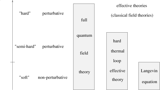
Figure 1: The full quantum field theory is necessary to describe the physics of all three relevant momentum scales, but it cannot be used for non-perturbative calculations. The hard thermal loop effective theory describes the physics of the scales $gT$ and $g^{2}T$. Due to Raleigh-Jeans UV divergences, it is difficult to treat non-perturbatively. By integrating out the scale $gT$, one obtains the Langevin equation which is free of UV problems.

3 Integrating out the hard modes

The hard modes constitute the bulk of degrees of freedom in the hot plasma. Their physics is that of almost free massless particles moving on straight lines. Even though they are weakly interacting, they have a significant influence on the soft dynamics because they are so numerous.

Integrating out the hard modes means that we have to calculate loop diagrams with external momenta $\ll T$ and internal momenta of order $T$. This generates effective propagators and vertices for the field modes with $p\ll T$. To leading order, we can neglect self-interactions of the hard modes. Therefore, we can restrict ourselves to one-loop diagrams. The leading one-loop contribution is due to the case that one propagator in the loop is on shell. For the remaining propagators one can use the high energy (or eikonal) approximation

$$\frac{1}{(Q+P)^{2}}=\frac{1}{2Q\cdot P+P^{2}}\simeq\frac{1}{2Q\cdot P}=\frac{1}{2q}\frac{1}{v\cdot P}.$$ (3.3)

Here $v=(1,{\bf v})$, where ${\bf v}={\bf q}/q$ is the 3-velocity of the hard particles. In this way one obtains the well known hard thermal loops $\!{}^{{\bf?}}$.

Before I proceed, let me give you an argument, due to Arnold, Son and Yaffe $\!{}^{{\bf?}}$, why hard thermal loops are relevant to the non-perturbative dynamics of the soft modes. For the electric, or longitudinal modes the effect of hard thermal loops is obvious. The longitudinal polarization tensor is of order $g^{2}T^{2}$ and is therefore much larger than $P^{2}$, when $P$ is of order $g^{2}T$. Thus electric interactions are screened on a length scale of order $(gT)^{-1}$.

The magnetic, or transverse modes are unscreened when $p_{0}$ is zero. This leads to the well known infrared problems in hot non-Abelian gauge theories. However, to compute unequal time correlation functions, one has to consider non-zero real $p_{0}$. Then, also the magnetic modes are screened. In order to avoid this screening, and to develop large, non-perturbative fluctuations, the soft modes have to move very slowly. The transverse propagator becomes unscreened when the hard thermal loop selfenergy $\delta\Pi_{\rm t}(P)$ becomes of order $p\sim g^{2}T$. In the small frequency limit $p_{0}\ll p$, we have

$$\delta\Pi_{\rm t}(P)\simeq-i\frac{\pi}{4}m^{2}_{\rm D}\frac{p_{0}}{p},$$ (3.4)

where $m^{2}_{\rm D}\sim(gT)^{2}$ is the leading order Debye mass. From this expression one can see that the frequency scale, at which the propagator becomes unscreened, is $p_{0}\sim g^{4}T$.

The main difference between Abelian and non-Abelian theories is that for the former the only hard thermal loop is the polarization tensor, while for the latter there are also hard thermal loop $n$-point functions for all $n$. As we will see below, this has a significant effect on the soft dynamics, it is in fact qualitatively different in Abelian and non-Abelian theories.

The hard thermal loop effective theory is described by the effective action

$$S_{\rm eff}=S+\Gamma_{\rm HTL},$$ (3.5)

where $\Gamma_{\rm HTL}$ is the generating functional of the hard thermal loop $n$-point functions. It is gauge invariant and non-local. The non-locality is due to the eikonal propagators like in Eq. (3.3).

As I discussed above, this effective theory is a classical field theory, since both $gT$ and $g^{2}T$ are small compared to $T$. Therefore, it is described by the classical equation of motion $\delta S_{\rm eff}/\delta A_{\mu}=0$. As the effective action itself, this equation of motion is non-local, which makes it difficult to deal with.

Figure 2: The relevant interactions between the different field modes. In the full theory, only the hard–semi-hard and hard–soft interactions contribute at leading order. Therefore, the relevant interactions within the hard thermal loop effective theory are due to hard thermal loop vertices.

Fortunately, there is a local formulation of the equations of motion due to Blaizot and Iancu $\!{}^{{\bf?}}$ and due to Nair $\!{}^{{\bf?}}$. It is the non-Abelian generalization of the linearized Vlasov equations for relativistic QED plasma. In addition to gauge fields, these equations contains a field $W(x,{\bf v})$ which lives in the adjoint representation. It describes the fluctuation of the distribution of hard particles with 3-velocity ${\bf v}$ (cf. Eq. (3.3)) around thermal equilibrium. The equation of motion for the gauge fields is

$$[D_{\mu},F^{\mu\nu}(x)] = m^{2}_{\rm D}\int\frac{d\Omega_{\bf v}}{4\pi}v^{\nu}W(x,{\bf v}).$$ (3.6)

The rhs is the current due to the hard particles. The equation for $W$ reads

$$[v\cdot D,W(x,{\bf v})] = {\bf v}\cdot{\bf E}(x),$$ (3.7)

where ${\bf E}$ is the (color-) electric field.

One may wonder, why one does not stop at this point and uses Eqs. (3.6), (3.7) for a lattice calculation. The reason is, that they suffer from Raleigh-Jeans UV divergences $\!{}^{{\bf?}}$. So far, no method has been found which cures these divergences in real time correlation functions. Fortunately, perturbation theory still works for momenta of order $gT$. Therefore, one can integrate out this scale and, at leading log accuracy, the resulting effective theory is free of UV problems.

4 Integrating out the semi-hard modes

The fields in the kinetic equations (3.6), (3.7) contain Fourier components with momenta of order $gT$ and $g^{2}T$. Now we split these fields into long- and short wavelength components. We introduce a separation scale $\mu$ such that

$$g^{2}T\ll\mu\ll gT.$$ (4.8)

The fields $A$, ${\bf E}$ and $W$ are decomposed into soft and a semi-hard modes ,

$$A\to A+a,\quad{\bf E}\to{\bf E}+{\bf e},\quad W\to W+w.$$ (4.9)

The soft fields $A$, ${\bf E}$ and $W$ contain the spatial Fourier components with $p<\mu$, while the semi-hard fields $a$, ${\bf e}$ and $w$ consist of those with $k>\mu$. Both $W$ and $w$ describe deviation of the distribution of the hard particles from thermal equilibrium. $W$ ($w$) is the slowly (rapidly) varying piece of this distribution varying on length scale greater (less) than $1/\mu$.

Integrating out the scale $gT$ means that we eliminate the semi-hard fields from the equations of motion for the soft ones. Then we will obtain equations of motion for the soft fields only .

After the split one obtains a set of coupled equations of motion for the soft and for the semi-hard fields. The low momentum part of Eq. (3.7) becomes

$$[v\cdot D,W(x,{\bf v})]={\bf v}\cdot{\bf E}(x)+\xi(x,{\bf v}),$$ (4.10)

where

$$\xi(x,{\bf v})=ig[v\!\cdot\!a(x),w(x,{\bf v})]_{\rm soft}.$$ (4.11)

The subscript “soft” indicates that only spatial Fourier components with $p<\mu$ are included.

I said that the semi-hard fields are perturbative. Here we are only interested in leading order results. Then one might expect, that one can approximate $\xi\simeq\xi_{0}$, where

$$\xi_{0}(x,{\bf v})=ig[v\!\cdot\!a_{0}(x),w_{0}(x,{\bf v})]_{\rm soft},$$ (4.12)

and $a_{0}$, $w_{0}$ are the solutions to the linearized kinetic equations. This is not quite correct, which will become clear in the moment. But for the sake of simplicity, let us assume that $\xi\simeq\xi_{0}$ is a good approximation, and consider the effect of $\xi_{0}$ in Eq. (4.10).

In order to compute correlation functions, one has to solve the equations of motion for the soft fields in the presence of $\xi_{0}$. Since these equations are non-linear, the solution will contain many factors of $\xi_{0}$. Now one has to perform the thermal average over initial conditions. One encounters expectation values like

$$\langle\xi_{0}(x_{1},{\bf v}_{1})\cdots\xi_{0}(x_{n},{\bf v}_{n})\rangle.$$ (4.13)

The typical separation of the points ${\bf x}_{1},\ldots,{\bf x}_{n}$ is of order $(g^{2}T)^{-1}$. In contrast, the fields $a_{0}$ and $w_{0}$ are correlated over a much smaller length scale of order $(gT)^{-1}$. Therefore, (4.13) factorizes into a product

$$\langle\xi_{0}(x_{1},{\bf v}_{1})\cdots\xi_{0}(x_{n},{\bf v}_{n})\rangle\simeq\langle\xi_{0}(x_{1},{\bf v}_{1})\rangle\cdots\langle\xi_{0}(x_{n},{\bf v}_{n})\rangle,$$ (4.14)

while connected parts are suppressed by some powers of the coupling constant. Now we will see why it is not sufficient to use the approximation $\xi\simeq\xi_{0}$. The rhs of Eq. (4.14) is zero! $\langle\xi_{0}^{a}\rangle$ contains the expectation value

$$\langle a_{0}^{b}w_{0}^{c}\rangle\propto\delta^{bc},$$ (4.15)

which is contracted the anti-symmetric structure constant $f^{abc}$. Therefore, in order to obtain the leading non-vanishing contribution for (4.13), one has to take into account connected 2-point functions of $\xi_{0}$. In other words, $\xi_{0}$ acts like a Gaussian noise.

Since the leading order contribution due to $\xi_{0}$ vanishes, one also has to take into account the first “sub-leading” term in $\xi$ itself, which will be denoted by $\xi_{1}$. It is linear in the soft fields, and, like $\xi_{0}$, it is bilinear in $a_{0}$ and $w_{0}$. However, in this case the thermal average (4.15) gives a non-zero contribution. Thus, at leading order, one can approximate

$$\xi(x,{\bf v})\simeq\xi_{0}(x,{\bf v})+\langle\!\langle\xi_{1}(x,v)\rangle\!\rangle,$$ (4.16)

where $\langle\!\langle\cdots\rangle\!\rangle$ denotes the average over initial conditions for $a_{0}$ and $w_{0}$.

Evaluating the 2-point function of $\xi_{0}$, one encounters a contribution which is logarithmically sensitive to the separation scale $\mu$. Keeping only this piece, one finds

$$\langle\xi_{0}^{a}(x_{1},{\bf v})\xi_{0}^{b}(x_{2},{\bf v}^{\prime})\rangle = -\frac{2Ng^{2}T^{2}}{m^{2}_{\rm D}}\log\left(\frac{gT}{\mu}\right)I({\bf v},{\bf v}^{\prime})$$ (4.17)

$$\delta^{ab}\delta^{4}(x_{1}-x_{2}),$$

with

$$I({\bf v},{\bf v}^{\prime})=-\delta^{(S^{2})}({\bf v}-{\bf v}^{\prime})+\frac{1}{\pi^{2}}\frac{({\bf v}\cdot{\bf v}^{\prime})^{2}}{\sqrt{1-({\bf v}\cdot{\bf v}^{\prime})^{2}}}.$$ (4.18)

Here, $\delta^{(S^{2})}$ is the delta function on the two dimensional unit sphere,

$$\int d\Omega_{{\bf v}^{\prime}}f({\bf v}^{\prime})\delta^{(S^{2})}({\bf v}-{\bf v}^{\prime})=f({\bf v}).$$ (4.19)

The term $\langle\!\langle\xi_{1}\rangle\!\rangle$ contains a piece which has the same $\mu$-dependence as (4.17). Inserting the result into Eq. (4.10), one finds

$$[v\cdot D,W(x,{\bf v})] = {\bf v}\cdot{\bf E}(x)+\xi_{0}(x,{\bf v})$$ (4.20)

$${}+Ng^{2}T\log\left(\frac{gT}{\mu}\right)\int\!\frac{d\Omega_{{\rm v}_{1}}}{4\pi}I({\bf v},{\bf v}_{1})W(x,{\bf v}_{1}).$$

Eq. (4.20) is a Boltzmann equation for the soft fluctuations of the particle distribution $W(x,{\bf v})$. The rhs contains a collision term which is due to the interactions with the semi-hard fields. The collision term is accompanied by the Gaussian white noise $\xi_{0}$, which is due to the thermal fluctuation of initial conditions of the fields with $k>\mu$.

For a QED plasma, there is no collision term at this order in the coupling constant. In this case the size of the collision term is determined by the transport cross section which corresponds to a mean free path of order order $(e^{4}T)^{-1}$. For a non-Abelian plasma the relevant mean free path $\!{}^{{\bf?}}$ is of order $(g^{2}T\log(1/g))^{-1}$. It is determined by the total cross section which is dominated by small angle scattering: Even a scattering process which hardly changes the momentum of a hard particle can change its color charge which is what is seen by the soft gauge fields.

5 Solving the Boltzmann equation

I will now argue, that, at leading logarithmic order, the lhs of Eq. (4.20) can be neglected. The argument goes as follows : The only spatial momentum scales which are left in the problem are $\mu$ and $g^{2}T$. The field modes we are ultimately interested in, are the ones which have only momenta of order $g^{2}T$. The cutoff dependence on the rhs must drop out after solving the equations of motion for the fields with spatial momenta smaller than $\mu$. Thus, after the $\mu$-dependence has cancelled, the logarithm must turn into $\log(gT/(g^{2}T))=\log(1/g)$.

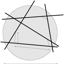
Figure 3: The non-perturbative dynamics is due to extended field configurations (shaded) with a typical size $R$ of order $(g^{2}T)^{-1}$. Since the soft fields are changing in time, they are associated with a long wavelength electric field. The hard modes behave like almost free particles moving on light-like trajectories (thick lines). They absorb energy from the long wavelength electric field which leads to the (Landau-) damping of the soft dynamics. The semi-hard field modes (thin lines) are responsible for color changing small angle scattering of the hard particles. In the leading log approximation (Sect. 5), the typical distance between these scattering events is small compared to $R$, so that the damping becomes local.

Then the Boltzmann equation can be solved in logarithmic accuracy, i.e., neglecting terms which are suppressed by inverse powers of $\log(1/g)$. The collision term on the rhs is logarithmically enhanced over the flow term on the lhs, and one can neglect the lhs altogether. In other words, the kinematic of the hard particles does not play a role in this approximation (for a physical picture, see Fig. 3). Multiplying (4.20) with $v^{i}$ and integrating over ${\bf v}$, one obtains

$$\frac{1}{3}E^{i}(x){}+\xi_{0}^{i}(x)-\frac{1}{4\pi}Ng^{2}T\log(1/g)W^{i}(x)=0,$$ (5.21)

where

$$W^{i}(x) = \int\!\frac{d\Omega_{{\rm v}}}{4\pi}v^{i}W(x,v),$$ (5.22)

$$\xi_{0}^{i}(x) = \int\!\frac{d\Omega_{{\rm v}}}{4\pi}v^{i}\xi_{0}(x,v).$$ (5.23)

Solving (5.21) for $W^{i}$, and inserting the result into Maxwell’s equation for the soft fields, the latter becomes (in $A_{0}=0$ gauge)

$$\ddot{A}^{i}+[D_{j},F^{ji}(x)]=-\gamma\dot{A}^{i}(x)+\zeta^{i}(x),$$ (5.24)

where the damping coefficient (or color conductivity $\!{}^{{\bf?}}$) is given by

$$\gamma=\frac{4\pi m^{2}_{\rm D}}{3Ng^{2}T\log(1/g)}.$$ (5.25)

The noise $\zeta^{i}$ is proportional to $\xi_{0}^{i}$,

$$\zeta^{i}(x)=\frac{4\pi m^{2}_{\rm D}}{Ng^{2}T\log(1/g)}\xi_{0}^{i}(x).$$ (5.26)

Its 2-point function can be obtained from Eq. (4.17),

$$\langle\zeta^{ia}(x_{1})\zeta^{jb}(x_{2})\rangle=2T\gamma\delta^{ij}\delta^{ab}\delta^{4}(x_{1}-x_{2}).$$ (5.27)

6 The Langevin equation

The equation of motion (5.24) describes an over-damped system. To see this, let us estimate the second term on the lhs. It contains two covariant space derivatives of the gauge fields. Each derivative is of order $g^{2}T$ . Thus, this term can be estimated as

$$[D_{j},F^{ji}]\sim g^{4}T^{2}{\bf A}.$$ (6.28)

For the damping term on the rhs we have

$$\gamma\dot{{\bf A}}\sim\frac{T}{\log(1/g)}\frac{{\bf A}}{t}.$$ (6.29)

where $t$ is the characteristic time scale of the soft fields. Comparing (6.28) and (6.29), we find

$$t^{-1}\sim g^{4}\log(1/g)T.$$ (6.30)

Therefore, the second time derivative in (5.24) is negligible, and the dynamics of the soft modes is correctly described by the Langevin equation

$$[D_{j},F^{ji}(x)]=-\gamma\dot{A}^{i}(x)+\zeta^{i}(x).$$ (6.31)

The innocent looking approximation of dropping the term $\ddot{{\bf A}}$ has an important effect. The effective theory described by Eqs. (6.31), (5.27) is no longer sensitive to an UV cutoff $\!{}^{{\bf?}}$. Therefore it has a continuum limit when used in lattice simulations.

7 The hot sphaleron rate

Now that we know that the soft non-perturbative dynamics of the gauge fields is correctly described by Eq. (6.31), and that there is no dependence on the UV cutoff, it is straightforward to estimate the parametric form of the hot sphaleron rate. There is only one length scale $R\sim(g^{2}T)^{-1}$, and only one time scale $t\sim(g^{4}\log(1/g)T)^{-1}$ left in the problem, so that we can estimate

$$\Gamma\sim\frac{1}{tR^{3}}\sim g^{10}\log(1/g)T^{4}.$$ (7.32)

Therefore, at leading logarithmic order, the hot sphaleron rate has the form

$$\Gamma=\kappa g^{10}\log(1/g)T^{4},$$ (7.33)

where $\kappa$ is a non-perturbative coefficient which does not depend on the gauge coupling and which has been determined by solving (6.31) on the lattice $\!{}^{{\bf?}}$.

8 Summary

We have obtained an effective theory for the non-perturbative dynamics of the soft field modes by integrating out the hard ($p\sim T$) and semi-hard modes ($p\sim gT$) in perturbation theory. This effective theory is described by the Langevin equation (6.31).

Furthermore, we have determined the parametric form of the hot electroweak baryon number violation rate at leading order. It contains a non-perturbative numerical coefficient which can be evaluated using Eq. (6.31).

Acknowledgment This work was supported in part by the TMR network “Finite temperature phase transitions in particle physics”, EU contract no. ERBFMRXCT97-0122.

References

- [1] G.D. Moore, these proceedings.
- [2] D. Bödeker, Phys. Lett. B 426, 351 (1998).
- [3] P. Arnold, these proceedings.
- [4] P. Arnold, D. Son and L.G. Yaffe, Phys. Rev. D 55, 6264 (1997).
- [5] E. Braaten and R. Pisarski, Nucl. Phys. B 337, 569 (1990); J. Frenkel and J.C. Taylor, Nucl. Phys. B 334, 199 (1990); J.C. Taylor and S.M.H. Wong, Nucl. Phys. B 346, 115 (1990).
- [6] J. P. Blaizot, E. Iancu, Nucl. Phys. B 417, 608 (1994).
- [7] V.P. Nair, Phys. Rev. D48, 3432 (1993).
- [8] D. Bödeker, L. McLerran and A. Smilga, Phys. Rev. D 52, 4675 (1995).
- [9] D. Bödeker, NBI-HE-99-04, hep-ph/9903478.
- [10] D. Bödeker, NBI-HE-99-13, hep-ph/9905239.
- [11] A. Selikhov, M. Gyulassy, Phys. Lett. B 316, 373 (1993).
- [12] P. Arnold, D. Son and L.G. Yaffe, UW/PT 98-10, MIT CTP-2779, hep-ph/9810216.