DESY 99-113

TAUP 2594 - 99

Screening Effects on $\mathbf{F_{2}}$
at Low $\mathbf{x}$ and $\mathbf{Q^{2}}$

E.  L e v i n ¹⁾

HEP Department
School of Physics and Astronomy
Raymond and Beverly Sackler Faculty of Exact Science
Tel Aviv University, Tel Aviv, 69978, ISRAEL
and
DESY Theory Group
22603, Hamburg, GERMANY

Talk, given at Ringberg Workshop: “New Trands in HERA Physics”, May 30 - June 4 ,1999

Abstract: In this talk we discuss how deeply the region of high parton densities has been studied experimentally at HERA. We show that the measurements of deep inelastic structure functions at HERA confirm our theoretical expectation that at HERA we face a challenging problem of understanding a new system of partons: quarks and gluons at short distances with so large densities that we cannot treat this system perturbatively. We collect all experimental indications and manifestations of specific properties of high parton density QCD.

1 What Are Shadowing Corrections?

In the region of low $x$ and low $Q^{2}$ we face two challenging problems which have to be resolved in QCD:

1. Matching of “hard” processes, that can be successfully described in perturbative QCD (pQCD), and “soft” processes, that should be described in non-perturbative QCD (npQCD), but actually, we have only a phenomenological approach for them;

2. Theoretical approach for the high parton density QCD (hdQCD) which we reach in the deep inelastic scattering at low $x$ but at sufficiently high $Q^{2}$. In this kinematic region we expect that the typical distances will be small but the parton density will be so large that a new non perturbative approach shall be developed for understanding this system.

We are going to advocate the idea that these two problems are correlated and the system of partons always passes the stage of hdQCD before ( at shorter distances ) it goes to the black box, which we call non-perturbative QCD and which, practically, we describe in old fashion Reggeon phenomenology. In spite of the fact that there are many reasons to believe that such a phenomenology could be even correct, the distance between Reggeon approach and QCD is so large we are loosing any taste of theory doing this phenomenology. In hdQCD we still have a small parameter ( running QCD coupling $\alpha_{S}$ ) and we can start to approach this problem using the developed methods of pQCD [1]. However, we should realize that the kernel of the hd QCD problems are non-perturbative one, and therefore, approaching hdQCD theoretically we are preparing a new training grounds for searching methods for npQCD.

First, let me recall that DIS experiment is nothing more than a microscope and we have two variables to describe its work. The first one is the resolution of the microscope, namely, $\Delta x\,\approx\,\,1/Q$ where $Q^{2}$ is the virtuality of the photon. It means that out microscope can see all constituents inside a target with the size larger that $\Delta x$. The second variable is time of observation. It sounds strange that we have this new variable, which we do not use, working with a medical microscope. However, we are dealing here with the relativistic system which can produce hadrons (partons). So, for everyday analogy, we should consider rather a box with flies which multiply and their number is, certainly, different in different moment of time. To estimate this time we can use the uncertainty principle $\Delta t\,\propto 1/\Delta E$ where $\Delta E$ is the change of energy, namely, $\Delta E=E_{initial}-E_{final}$, and for system of quark and antiquark $\Delta E=q_{0}-q_{1}-q_{2}=q_{0}-q=\frac{(q_{0}-q)(q_{0}+q)m}{2q_{0}m}=\frac{Q^{2}m}{W^{2}}=mx$, where $m$ is mass of the target and $q_{0}$ and $q$ is the energy and momentum of the virtual photon. Finally, $t=1/mx$ with $x=\frac{Q^{2}}{W^{2}}$ where $W$ is the energy of photon - target interaction.

Therefore, the question, that we are asking in DIS at low $x$, is what happens with constituents of rather small size after long time. It is clear that the number of these constituents should increase since in QCD each parton can decay in two partons with the probability $P_{i}=\frac{N_{c}\alpha_{S}}{\pi}\frac{dE_{i}}{E_{i}}\,\frac{d^{2}k_{i,t}}{k^{2}_{i,t}}$ where $E_{i}$ and $\vec{k}_{i}$ are energy and momentum of an emitted parton $i$.

This growth we can describe introducing so called structure function ( $xG(x,Q^{2})$ ) or the number of partons that can be resolved with the microscope with definite $Q^{2}$ and $x$. Indeed,

$$\frac{\partial^{2}xG(x,Q^{2})}{\partial\ln(1/x)\,\partial\ln Q^{2}}\,\,=\,\,\frac{N_{c}\alpha_{S}}{\pi}xG(x,Q^{2})\,\,.$$ (1)

This equation is the DGLAP[2] evolution equation in the region of low $x$. It has an obvious solution $xG(x,Q^{2})\,\propto\,exp\left(2\sqrt{\frac{N_{c}\alpha_{S}}{\pi}\,\ln(1/x)\,\ln(Q^{2}/Q^{2}_{0})}\right)$. Therefore, we expect the increase of the parton densities at $x\,\rightarrow 0$.

In Fig. 1 we picture the parton distributions in the transverse plane. At $x\approx 1$ there are several partons of a small size. The distance between partons is much larger than their size and we can neglect interactions between them.

Figure 1: Parton distribution in the transverse plane

However, at $x\,\rightarrow\,0$ the number of partons becomes so large that they are populated densely in the area of a target. In this case, you cannot neglect the interactions between them which was omitted in the evolution equations ( see Eq. ( 1 ) ). Therefore, at low $x$ we have a more complex problem of taking into account both emission and rescatterings of partons. Since the most important in QCD is the three parton interaction, the processes of rescattering is actually a process of annihilation in which one parton is created out of two partons (gluons).

Therefore, at low $x$ we have two processes

1. Emission induced by the QCD vertex $G+G\rightarrow G$ with probability which is proportional to $\alpha_{S}\,\rho$ where $\rho$ is the parton density in the transverse plane , namely

   $$\rho=\frac{xG(x,Q^{2})}{\pi R^{2}}\,\,,$$ (2)

   where $\pi R^{2}$ is the target area;

2. Annihilation induced by the same vertex $G+G\rightarrow G$ with probability which is proportional to $\alpha_{S}\sigma_{0}\,\rho^{2}$, where $\alpha_{S}$ is probability of the processes $G+G\rightarrow G$, $\sigma_{0}$ is the cross section of two parton interaction and $\sigma_{0}\propto\,\frac{\alpha_{S}}{Q^{2}}$. $\sigma_{0}\,\rho$ gives the probability for two partons to meet and to interact, while $\alpha_{S}\sigma_{0}\,\rho^{2}$ gives the probability of the annihilation process.

Finally, the change of parton density is equal to [1] [3]

$$\frac{\partial^{2}\rho(x,Q^{2})}{\partial\ln(1/x)\,\partial\ln Q^{2}}\,\,=\,\,\frac{N_{c}\alpha_{S}}{\pi}\rho(x,Q^{2})\,\,-\,\,\frac{\alpha^{2}_{S}\gamma}{Q^{2}}\,\rho^{2}(x,Q^{2})\,\,$$ (3)

or in terms of the gluon structure function

$$\frac{\partial^{2}xG(x,Q^{2})}{\partial\ln(1/x)\,\partial\ln Q^{2}}\,\,=\,\,\frac{N_{c}\alpha_{S}}{\pi}xG(x,Q^{2})\,\,-\,\,\frac{\alpha^{2}_{S}\gamma}{\pi R^{2}Q^{2}}\,\left(xG(x,Q^{2})\right)^{2}\,\,,$$ (4)

where $\gamma$ has been calculated in pQCD [3].

Therefore, Eq.( 4 ) is a natural generalization of the DGLAP evolution equations. The question arises, why we call shadowing and /or screening corrections such a natural equation for a balance of partons due to two competing processes. To understand this let us consider the interaction of the fast hadron with the virtual photon at the rest ( Bjorken frame ). In the parton model, only the slowest ( “wee” ) partons interact with the photon. If the number of the “wee” partons $N$ is not large, the cross section is equal to $\sigma_{0}N$. However, if we have two “wee” partons with the same energies and momenta, we overestimate the value of the total cross section using the above formula. Indeed, the total cross section counts only the number of interactions and, therefore, in the situation when one parton is situated just behind another we do not need to count the interaction of the second parton if we have taken into account the interaction of the first one. It means that the cross section is equal to

$$\sigma_{tot}\,\,=\,\,\sigma_{0}N\,\{\,\,1\,\,-\,\,\frac{\sigma_{0}}{\pi R^{2}}\,\,\}\,\,,$$ (5)

where $R$ is the hadron radius. One can see that we reproduce Eq.( 4 ) by taking into account that there is a probability for a parton not to interact being in a shadow of the second parton.

2 What Have We Learned about SC?

During the past two decades high parton density QCD has been under the close investigation of many theorists [1] [3][4][5] and we summarize here the result of their activity.

• The parameter which controls the strength of SC has been found and it is equal to

  $$\kappa\,\,\,=\,\,\,\frac{3\,\pi^{2}\alpha_{s}}{2Q^{2}}\,\times\,\frac{xG(x,Q^{2})}{\pi\,R^{2}}\,\,\,=\,\,\,\sigma_{0}\,\times\,\rho(x,Q^{2})\,\,.$$ (6)

  The meaning of this parameter is very simple. It gives the probability of interaction for two partons in the parton cascade or, better to say, a packing factor for partons in the parton cascade.

• We know the correct degrees of freedom at high energies: colour dipoles [6]. By definition, the correct degrees of freedom is a set of quantum numbers which mark the wave function that is diagonal with respect to interaction matrix. Therefore, we know that the size and the energy of the colour dipole are not changed by the high energy QCD interaction.

• A new scale $Q^{2}_{0}(x)$ for hdQCD has been traced in pQCD approach which is a solution to the equation

  $$\kappa\,\,\,=\,\,\,\frac{3\,\pi^{2}\alpha_{s}}{2Q^{2}_{0}(x)}\,\times\,\frac{xG(x,Q^{2}_{0}(x))}{\pi\,R^{2}}\,\,=\,\,1\,\,.$$ (7)

  This new scale leads to the effective Lagrangian approach which gives us a general non-perturbative method to study hdCD.

• We know that the GLR equation ( see Eqs.( 3 ) and ( 4) ) describes the evolution of the dipole density in the full kinematic region [7]. We understood that the Mueller-Glauber approach for colour dipole rescattering gives the initial condition to the GLR equation.

• The new, non-perturbative approach, based on the effective Lagrangian [5], have been developed for hdQCD which gives rise to the hope that hdQCD can be treated theoretically from the first principles.

• We are very close to understanding of the parton density saturation [1].

In general, we think that the theoretical approach to hdQCD in a good shape now.

3 HERA Puzzle: Where Are SC?

The wide spread opinion is that HERA experimental data for $Q^{2}\,\geq\,1\,GeV^{2}$ can be described quite well using only the DGLAP evolution equations, without any other ingredients such as shadowing corrections, higher twist contributions and so on ( see. for example, reviews [8] ). On the other hand, the most important HERA discovery is the fact that the density of gluons ( gluon structure function ) becomes large in HERA kinematic region [8][9]. The gluon densities extracted from HERA data is so large that parameter $\kappa$ ( see Eq.( 6) ) exceeds unity in substantial part of HERA kinematic region (see Fig.2a ). Another way to see this is to plot the solution to Eq.( 7) ( see Fig.2b). It means that in large kinematic region $\kappa\,\geq\,1$ ( to the left from line $\kappa=1$ in Fig.2b), we expect that the SC should be large and important for a description of the experimental data. At first sight such expectations are in a clear contradiction with the experimental data. Certainly, this fact gave rise to the suspicions or even mistrusts that our theoretical approach to SC is not consistent. However, the revision and re-analysis of the SC , as has been discussed in the previous section, have been completed with the result, that $\kappa$ is responsible for the value of SC.

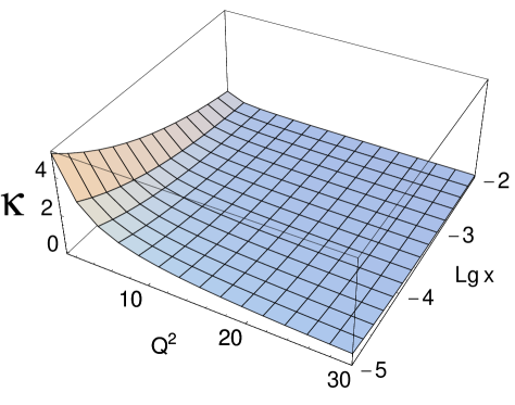
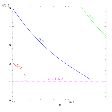
Fig.2a	Fig.2b

Figure 2: Parameter $\kappa$ and new scale $Q^{2}_{0}(x)$.

Therefore, we face a puzzling question: where are SC?. Actually, this question includes, at least, two questions: (i) why SC are not needed to describe the HERA data on $F_{2}$, and (ii) where are the experimental manifestation of strong SC. The answers for these two questions you will find in the next three sections but, in short, they are: SC give a weak change for $F_{2}$ in HERA kinematic region, but they are strong for the gluon structure function . We hope to convince you that there are at least two indications in HERA data supporting a large value of SC to gluon density:

1. $x_{P}$ - behaviour of the cross section of the diffractive dissociation ($\sigma^{DD}$) in DIS;

2. $Q^{2}$ - behaviour of $F_{2}$ -slope ( $\frac{\partial F_{2}(x,Q^{2})}{\partial\ln Q^{2}}$ ).

4 SC for $\mathbf{F_{2}}$

It is well known, that $\gamma^{*}$ - hadron interaction goes in two stages: (i) the transition from virtual photon to colour dipole and (ii) the interaction of the colour dipole with the target. To illustrate how SC work, we consider the Glauber - Mueller formula which describes the rescatterings of the colour dipole with the target[10]:

$$F_{2}(x_{B},Q^{2})\,\,\, = \frac{N_{c}}{6\pi^{3}}\,\sum^{N_{f}}_{1}\,Z^{2}_{f}\,\,\int^{Q^{2}}_{Q^{2}_{0}}\,\,dQ^{\prime 2}\int db^{2}_{t}\{\,\,1\,\,\,-\,\,\,e^{-\frac{1}{2}\frac{4}{9}\,\kappa(x_{B},Q^{\prime 2})\,S(b_{t})}\,\,\}\,\,$$ (8)

$$+ \,\,F_{2}(x_{B},Q^{2}_{0})\,,$$

where $S(b_{t})=e^{-\frac{b^{2}_{t}}{R^{2}}}$ is the target profile function in the impact parameter representation and $\frac{4}{9}\,\kappa(x_{B},Q^{\prime 2})=\sigma(x_{B},r^{2}_{\perp}=4/Q^{2})$ is the cross section of the dipole scattering in pQCD.

One can see that Eq.( 8) leads to

$$F_{2}(x_{B},Q^{2})\,\,\longrightarrow\,\,\frac{N_{c}}{6\pi^{3}}\,\sum^{N_{f}}_{1}\,Z^{2}_{f}\,\,Q^{2}R^{2}\,\,.$$ (9)

However, we are sure that the kinematic region of HERA is far away from the asymptotic one. The practical calculations depend on three ingredients: the value of $R^{2}$, the value of the initial virtuality $Q^{2}_{0}$ and the initial $F_{2}$ at $Q^{2}_{0}$. We fix them as follows: $R^{2}=10\,GeV^{-2}$ which corresponds to “soft” high energy phenomenology [11], $Q^{2}_{0}=1\,GeV^{2}$ and $F^{input}_{2}(x_{B},Q^{2}_{0})=F^{GRV^{\prime}94}_{2}(x_{B},Q^{2}_{0}=1\,GeV^{2})$. Therefore, the result of calculation should be read as “SC for colour dipoles with the size smaller than $r^{2}_{\perp}\,\leq\,4/1GeV^{2}$ are equal to …”

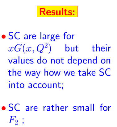
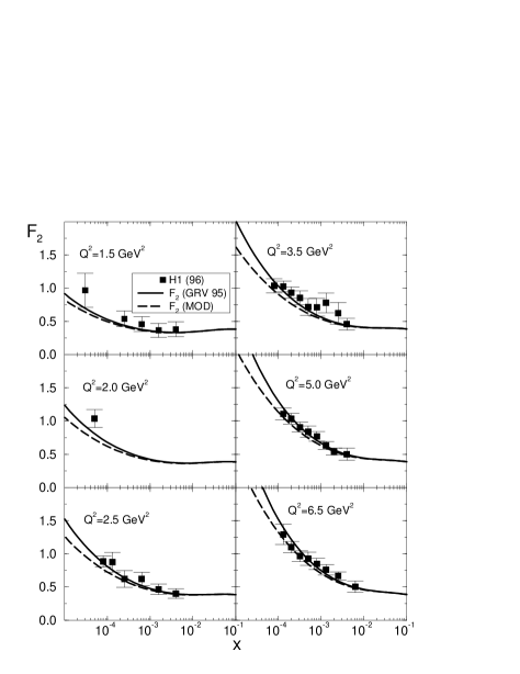
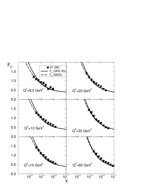
Figure 3: SC for $xG(x,Q^{2})$ and $F_{2}$ in the HERA kinematic region .

From Fig.3 one can see that the SC are rather small for $F_{2}$ but they are strong and essential for the gluon structure function. It means that we have to look for the physics observables which will be more sensitive to the value of the gluon structure function than $F_{2}$.

5 $\mathbf{x_{P}}$- dependence of $\mathbf{\sigma^{DD}}$

One of such observables is the cross section of the diffractive dissociation and, especially, the energy dependence of this cross section.

Data: Both H1 and ZEUS collaborations [8] found that

$$\sigma^{DD}\,\,\propto\,\,\frac{1}{x^{2\Delta_{P}}}\,\,,$$ (10)

where $\Delta_{P}=\alpha_{P}(0)-1$ and the values of $\alpha_{P}(0)$ are:

• H1  [12]   :     $\alpha_{P}(0)$ = 1.2003 $\pm$ 0.020(stat.) $\pm$ 0.013(sys) ;

• ZEUS [13] :  $\alpha_{P}(0)$ = 1.1270 $\pm$ 0.009(stat.) $\pm$ 0.012(sys) .

It is clear that the Pomeron intercept ($\alpha_{P}(0)$) for diffractive processes in DIS is higher than the intercept of “soft” Pomeron [11].

Why is it surprising and interesting? To answer this question we have to recall that the cross sections for diffractive production of quark-antiquark pair have the following form in pQCD [14] [15]:

$$x_{P}\,\frac{d\sigma^{T}_{DD}(\gamma^{*}\,\rightarrow\,q+\bar{q})}{dx_{P}dt}\,\, \,\propto\, \int^{\frac{M^{2}}{4}}_{Q^{2}_{0}}\,\,\frac{dk^{2}_{\perp}}{k^{2}_{\perp}}\,\,\times\,\,\frac{\left(\,\alpha_{S}\,\,x_{P}\,G(x_{P},\frac{k^{2}_{\perp}}{1-\beta})\,\right)^{2}}{k^{2}_{\perp}}\,;$$ (11)

$$x_{P}\,\frac{d\sigma^{L}_{DD}(\gamma^{*}\,\rightarrow\,q+\bar{q})}{dx_{P}dt}\,\, \,\propto\, \,\int^{\frac{M^{2}}{4}}_{Q^{2}_{0}}\,\,\frac{dk^{2}_{\perp}}{Q^{2}}\,\,\times\,\,\frac{\left(\,\alpha_{S}\,\,x_{P}\,G(x_{P},\frac{k^{2}_{\perp}}{1-\beta})\,\right)^{2}}{k^{2}_{\perp}}.$$ (12)

From Eqs.( 11) and ( 12) you can see that $k_{\perp}$ integration looks quite differently for transverse and longitudinal polarized photon: the last one has a typical log integral over $k_{\perp}$ while the former has the integral which normally converges at small values of $k_{\perp}$. We have the same property for production a more complex system than $q\bar{q}$, for example $q\bar{q}G$ [15]. Therefore, we expect that the diffractive production should come from long distances where the “soft” Pomeron contributes. However, the experiment says a different thing, namely, that this production has a considerable contamination from short distances. How is it possible? As far as we know, there is the only one explanation: SC are so strong that $xG(x,k^{2}_{\perp})\,\,\propto\,\,k^{2}_{\perp}R^{2}$ (see Eq.( 9) ) Substituting this asymptotic limit in Eq.( 11) one can see that the integral becomes convergent and it sits at the upper limit of integration which is equal to $k^{2}_{\perp}=Q^{2}_{0}(x)$.

Finally, we have

$$x_{P}\,\frac{d\sigma_{DD}}{dx_{P}dt}\,\,\,\longrightarrow\,\,\,\,\left(\,x_{P}\,G(x_{P},Q^{2}_{0}(x_{P}))\,\right)^{2}\,\,\times\,\,\frac{1}{Q^{2}_{0}(x_{P})}$$ (13)

The calculation for $\frac{\partial xG(x,Q^{2})}{\partial\ln(1/x)}$ is given in Fig.4 for HERA kinematic region using Glauber-Mueller formula [10] for SC. Taking into account that $Q^{2}_{0}(x)$ in Fig.2b can be fitted as $Q^{2}_{0}(x)\,\,\,=\,\,1\,\,GeV^{2}\,\left(\,\frac{x}{x_{0}}\,\right)^{-\lambda}$ with $\lambda=0.54$ and $x_{0}=10^{-2}$ we see from Eq.( 13) and Fig.4 that we are able to reproduce the experimental value of $\alpha_{P}(0)$ and conclude that the typical $k^{2}_{\perp}$ which are dominant in the integral is not small ( $k^{2}_{\perp}\,\,\approx\,\,1-2\,GeV^{2}$ [15] ). For Golec-Biernat and Wüsthoff approach, which we will discuss late, $\lambda=0.288$ and the value of typical $k^{2}_{\perp}$ turns out to be higher.

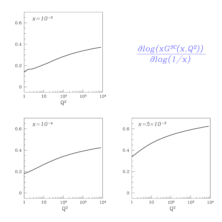
Figure 4: Effective Pomeron intercept for gluon structure function calculated using Glauber-Mueller formula for SC

6 The $\mathbf{Q^{2}}$- dependence of the $\mathbf{F_{2}}$ - slope.

Data: The experimental data [13] for $F_{2}$ - slope $dF_{2}(x,Q^{2})/d\ln Q^{2}$ are shown in Fig.5a (Caldwell plot). These data give rise to a hope that the matching between “hard” ( short distance) and “soft” (long distance) processes occurs at sufficiently large $Q^{2}$ since the $F_{2}$-slope starts to deviate from the DGLAP predictions around $Q^{2}\,\approx\,5-8\,GeV^{2}$.

$\mathbf{F_{2}}$-slope and SC: Our principle idea, as we have mentioned in the beginning of the talk, is that matching between “hard” and “soft” processes is provided by the hdQCD phase in the parton cascade or, in other words, due to strong SC. The asymptotic behaviour of $F_{2}\,\propto\,Q^{2}R^{2}$ for $Q^{2}\,\leq\,Q^{2}_{0}(x)$ leads to $dF_{2}(x,Q^{2})/d\ln Q^{2}\,\propto\,Q^{2}R^{2}$ at $Q^{2}\,\leq\,Q^{2}_{0}(x)$ (see Eq.( 9) ) and this behaviour supports our point of view [16][17].

However, we have two problems to solve before making any conclusion: (i) the experimental data are taken at different points $(x,Q^{2})$ and therefore could be interpreted as the change of $x$-behaviour rather than $Q^{2}$ one; and (ii) the value of $F_{2}$-slope is quite different from the value of $F_{2}$ while for the asymptotic solution it should be the same. Therefore, we have to calculate $F_{2}$ - slope to understand them. The result of calculation using the Glauber-Mueller formula [16] is presented in Fig.5b. One can see that (i) the experimental data shows rather $Q^{2}$ - behaviour then the $x$-dependence, which is not qualitatively influenced by SC; and (ii) SC are able to describe both the value and the $Q^{2}$-behaviour of the experimental data. Fig.5b shows also that the ALLM’97 parameterization [18], which can be viewed as the phenomenological description of the experimental data, has the same features as our calculation confirming the fact that the data show $Q^{2}$ - dependence but not $x$-behaviour of the $F_{2}$-slope.

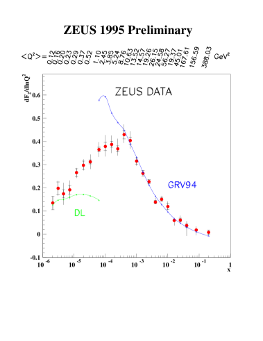
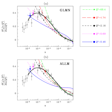
Fig.5a	Fig.5b

Figure 5: $F_{2}$-slope: experimental data (Caldwell plot ) (Fig.5a) and calculations using Glauber-Mueller formula (Fig.5b) .

7 Golec-Biernat and Wüsthoff Approach

Golec-Biernat and Wüsthoff [19] suggested a phenomenological approach which takes into account the key idea of hdQCD, namely, the new scale of hardness in the parton cascade. They use for $\gamma^{*}p$ cross section the following formula [19]

$$\sigma_{tot}(\gamma^{*}p)\, = \,\int d^{2}r_{\perp}\int^{1}_{0}\,dz\,|\Psi(Q^{2};r_{\perp},z)|^{2}\,\,\sigma_{tot}(r^{2}_{\perp},x)\,\,;$$ (14)

$$\sigma(x,r_{\perp})\, = \,\sigma_{0}\,\,\{\,\,1\,\,\,-\,\,\,e^{-\,\frac{r^{2}_{\perp}}{R^{2}(x)}}\,\,\}\,\,;$$ (15)

$$R^{2}(x)\, = \,1/Q^{2}_{0}(x)\,\,\,\,with\,\,\,Q^{2}_{0}(x)\,\,=\,\,Q^{2}_{0}\,\left(\,\frac{x}{x_{0}}\,\right)^{-\lambda}\,\,.$$ (16)

Extracting parameters of their model from fitting of the experimental data, namely, $\sigma_{0}$=23.03 mb, $\lambda$ = 0.288, $Q^{2}_{0}=1GeV^{2}$ and $x_{0}$ = 3.04 $10^{-4}$ , they described quite well all data on total and diffractive cross sections in DIS (see Fig.6 ).

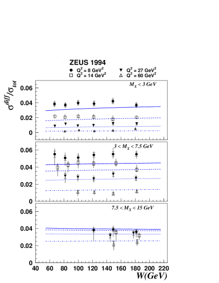
Fig.6a	Fig.6b

Figure 6: $\sigma_{tot}(\gamma^{*}p)$ amnd the ration $\sigma^{DD}/\sigma_{tot}$ for DIS in Golec-Biernat and Wüsthoff model. Vertical line in Fig.6a is the $Q^{2}_{0}(x)$ given by Eq.(16).

8 Why Have We Only Indications?

The answer is: because we have or can have an alternative explanation of each separate fact. For example, we can describe the $F_{2}$ -slope behaviour changing the initial $x$-distribution for the DGLAP evolution equations [20]. Our difficulties in an interpretation of the experimental data is seen in Fig.6a where the new scale $Q^{2}_{0}(x)$ is plotted. One can see that $Q^{2}_{0}(x)$ is almost constant in HERA kinematic region. It means that we can put the initial condition for the evolution equation at $Q^{2}_{0}=<Q^{2}_{0}(x)>$ where $<Q^{2}_{0}(x)>$ is the average new scale in HERA region. Therefore, SC can be absorbed to large extent in the initial condition and the question, that can and should be asked, is how well motivated these conditions are. For example, I do not think that initial gluon distribution in MRST parameterization [20], needed to describe the $F_{2}$ - slope data, can be considered as a natural one.

9 Summary

We hope we convinced you that (i) hdQCD is in a good theoretical shape; (ii) the hdQCD region has been reached at HERA; (iii) HERA data do not contradict the strong SC effects; (iv) there are at least two indications on SC effects in HERA data: $Q^{2}$ behaviour of $F_{2}$ slope and $x_{P}$ behaviour of diffractive cross section in DIS; and (v) the HERA data and the hdQCD theory gave an impetus for a very successful phenomenology for matching “hard” and “soft” physics.

We would like to finish this talk with rather long citation: “Small $x$ Physics is still in its infancy. Its relations to heavy ion physics, mathematical physics and soft hadron physics along with a rich variety of possible signature makes it central for QCD studies over the next decade” ( A.H. Mueller, B. Müller, G. Rebbi and W.H. Smith “Report of the DPF Long Range Planning WG on QCD”). Hopefully, we will learn more on low $x$ physics by the next Ringberg Workshop.

References

- [1] L. V. Gribov, E. M. Levin and M. G. Ryskin: Phys.Rep. 100, 1 (1983).
- [2] V.N. Gribov and L.N. Lipatov: Sov. J. Nucl. Phys. 15,438 (1972); L.N. Lipatov: Yad. Fiz. 20, 181 (1974; G. Altarelli and G. Parisi: Nucl. Phys. B 126, 298 (1977); Yu.L. Dokshitser: Sov. Phys. JETP 46, 641 (1977).
- [3] A.H. Mueller and J. Qiu: Nucl. Phys. B 268, 427 (1986).
- [4] E. Laenen and E. Levin: Ann. Rev. Nucl. Part. 44, 199 (1994) and references therein; A.H. Mueller: Nucl. Phys. B 437, 107 (1995); G. Salam: Nucl. Phys. B 461, 512 (1996); A.L. Ayala, M.B. Gay Ducati and E.M. Levin: Nucl. Phys. B 493, 305 (1997) (1997); 510, 355 (1998).
- [5] L. McLerran and R. Venugopalan: Phys. Rev. D 49,2233,3352 (1994); 50, 2225 (1994); 53,458 (1996); J. Jalilian-Marian, A. Kovner, A. Leonidov and H. Weigert: Phys. Rev. D 59,014014, 034007 (1999); J.Jalilian-Marian, A. Kovner, L. McLerran and H. Weigert: Phys. Rev. D 55, 5414 (1997); A. Kovner, L. McLerran and H. Weigert: Phys. Rev. D 52, 3809,6231 (1995); Yu. Kovchegov: Phys. Rev. D 54,5463 (1996); 55,5445 (1997); Yu. V. Kovchegov and A.H. Mueller: Nucl. Phys. B 529, 451 (1998); Yu. V. Kovchegov, A.H. Mueller and S. Wallon: Nucl. Phys. B 507, 367 (1997).
- [6] A.H. Mueller: Nucl. Phys. B 425.471 (1994).
- [7] Yuri V. Kovchegov: Small Structure Function of a Nucleus Including Multiple Pomeron Exchange, NUC-MN-99/1-T, hep-ph/9901281.
- [8] A.M. Cooper-Sarkar, R.C.E. Devenish and A. De Roeck: Int.J.Mod.Phys. A 13, 3385 (1998); H.Abramowicz and A. Caldwell: HERA Collider Physics DESY-98-192, hep-ex/9903037, Rev. Mod. Phys. (in press ).
- [9] ZEUS Collaboration, J. Breitweg et al.: Eur. Phys. J. C 7,609 (1999).
- [10] A. H. Mueller: Nucl. Phys. B 335, 115 (1990).
- [11] A. Donnachie and P.V. Landshoff: Nucl.Phys. B 244, 322 (1984; 267, 690 (1986); Phys. Lett. B 296, 227 (1992; Z. Phys. C 61, 139 (1994); E. Gotsman,E. Levin and U. Maor: Phys. Lett. B 452, 287 (1999),304,199 (1992) ; Phys. Rev. D 49, 4321 (1994); Z. Phys. C 57,672 (1993).
- [12] H1 Collaboration, T. Ahmed et al.: Phys. Lett. B 348, 681 (1995); C. Adloff et al.: Z. Phys. C 76, 613 (1997).
- [13] ZEUS Collaboration, M. Derrick et al.: Z. Phys. C 68, 569 (1995); J. Breitweg et al.: Eur. Phys. J. C 6, 43 (1999).
- [14] J. Bartels, H. Lotter and M. Wüsthoff: Phys. Lett. B 379, 239 (1996) and references therein.
- [15] E. Gotsman,E. Levin and U. Maor: Nucl. Phys. B 493, 354 (1997).
- [16] E. Gotsman,E. Levin and U. Maor: Phys. Lett. B 425, 369 (1998); E. Gotsman, E. Levin, U. Maor and E. Naftali: Nucl. Phys. B 539, 535 (1999).
- [17] A.H. Mueller: Small and Diffraction Scattering, DIS’98, eds. Ch. Coremans and R. Roosen, WS,1998, Parton Saturation at Small and in Large Nuclei, CU-TP-937-99, hep-ph/9904404.
- [18] H. Abramowicz, E. Levin, A. Levy and U. Maor: Phys. Lett. B 269, 465 (1991); H. Abramowicz and A. Levy: ALLM’97, DESY 97 -251, hep-ph/9712415.
- [19] K. Golec-Biernat and M. Wüsthoff: Phys. Rev. D 59, 014017 (1999); Saturation in Diffractive Deep Inelastic Scattering, DTP-99-20,hep-ph/9903358.
- [20] A.D. Martin, R.G. Roberts, W.J. Stirling and R.S. Thorne: Parton Distributions and the LHC: W and Z Production, DTP-99-64, hep-ph/9907231.