Intermediate-Mass Higgs Searches in Weak Boson Fusion

missing

Weak boson fusion is a copious source of intermediate mass Higgs bosons at the LHC. The additional very energetic forward jets in these events are powerful background suppression tools. I analyze the decays $H\to\gamma\gamma$ and $H\to W^{(*)}W^{(*)}\to e^{\pm}\mu^{\mp}/\!\!\!p_{T}$, with the latter a potential discovery channel, and the decay $H\to\tau^{+}\tau^{-}\to\ell^{\pm}h^{\mp}/\!\!\!p_{T}$ as a method for achieving the first direct measurement of a Higgs-fermion coupling.

I perform parton level analyses of the signal and dominant backgrounds for each decay mode, and demonstrate kinematic cuts and other important tools neccessary to achieve an S/B $>1/1$ rate in all cases. I also perform cross section calculations with additional gluon emission which provide an estimate of a minijet veto probability.

I show that a $5\sigma$ $H\to\gamma\gamma$ observation can be made for 110 GeV $<M_{H}<$ 150 GeV with modest luminosity, order 40-50 fb^-1 at low machine luminosity, overlapping the region explored by the CERN LEP and Fermilab Tevatron. For 130 GeV $<M_{H}<$ 200 GeV, I show that $H\to W^{(*)}W^{(*)}$ can achieve a $5\sigma$ observation with S/B much greater than 1/1 with extremely low luminosity, about 2-10 fb^-1 over almost the entire range. This is the most promising search channel in the 130-200 GeV mass range. It overlaps the $H\to\gamma\gamma$ region and nicely complements the $H\to W^{(*)}W^{(*)}$ measurement that can be made with very low luminosity in inclusive $gg\to H$ production. I further show that a Higgs-fermion coupling can be directly measured via the $H\to\tau\tau$ decay with only about 60 fb^-1 (assuming low luminosity running).

missing

I am most indebted to my advisor, Dieter Zeppenfeld, for both his teaching of physics and the extraordinary patience and kindness it surely took to withstand the onslaught of questions to which I subjected him, especially the repeated ones and especially early on. I am grateful he agreed to take me on as an apprentice, and only hope I can one day try to hold the same standards of mentoring for my students.

I thank the rest of the Phenomenology Institute professors, Vernon Barger, Francis Halzen, Tao Han and Martin Olsson, for their support and the friendly atmosphere they maintain in these halls. I did well to choose Wisconsin for my studies.

I will long remember the camaraderie shared with my fellow high-energy students and colleagues John Beacom, Tim Kinnel, Nikolas Kauer and Bill Long, as well as with our wonderful librarian Kerry Kresse, in everything from rag sessions about physics, computers, or people and politics, to a passion for flying. I thank my fellow students, most notably Steve Kadlecek, Rob Haslinger, Chris O’Dell, Brian Schwartz and Greg Jaczko, for the late-night Jackson problem-solving sessions that helped me make it this far, and the great parties after every ordeal we endured.

I owe thanks to my colleagues outside of the Phenomenology Institute with whom I was lucky to have worked while still a graduate student, Kaoru Hagiwara, Tim Stelzer and Rob Szalapski. Their advice and encouragement has been invaluable.

I thank my former teachers Keith Vemmer and Mark Schuermann, who first sparked my interest in science, and my undergraduate physics professors Cliff Tompson, David Cowan, Meera Chadrasekhar and the late Justin Huang, for planting my feet firmly on the path to a career in physics.

Finally, I cannot forget my parents Gary and Becky, whom I thank for supporting me in pursuing a goal that I think cannot be reached without an endless supply of encouragement.

Contents

toc

List of Figures

lof

List of Tables

lot

Chapter 1 Introduction

1.1 Where Are We?

The year 1999 finds the particle physics community on the cusp of understanding the fundamental particles and forces of nature. We have, over the past three decades, formulated a theory governing the electromagnetic, weak and strong forces and their constituents, called the Standard Model, which now predicts with uncanny accuracy the results of most particle physics experiments, and there is a considerable volume of data with which to compare [?]. During this time numerous observations have been made that suggested new physics beyond the Standard Model, or that it was wrong, but all have essentially vanished as statistical fluctuations or experimental flaws.

Yet while the community continually rejoices in the predictive success of the Standard Model, it also faces the somber realization that the theory is unsatisfactory, that it is incomplete at a fundamental level. Aside from the deeper questions of the large number of input parameters required to define the theory (of order 20) [?], the intimation of unification of forces at energy scales higher than can be probed [?], and perhaps even the necessity of such principles as renormalizability, there are the more immediate problems of electroweak symmetry breaking (ESB) and mass generation, on which this dissertation focuses.

The Standard Model hinges on an explanation of these observations at a time when the community is on the verge of having the technical capability of exploring some of these issues with conclusion. It remains to be seen whether or not the Higgs mechanism, the (currently) most viable explanation of ESB, is correct. It is certain that this area has not yet been fully explored phenomenologically, and this dissertation outlines strategies for experimental searches designed to lay the issue to rest with efficiency and certainty.

In this Chapter, I introduce the physics of the electroweak sector of the Standard Model which describes all presently known interactions and forces other than gravity, explaining its structure and the mathematical limitations in formulating the theory with only the particles observed in nature. I describe how the observed ESB of the theory can be obtained via addition of a simple Higgs sector, and show the Standard Model couplings that result. I explain the origin of mass in the theory, for both known particles and the theoretically introduced but unobserved Higgs scalar, and why a light Higgs mass is expected from radiative corrections to the masses of the weak gauge bosons in light of the current status of electroweak (EW) precision fits to data. As a prelude to introduction of the minijet veto tool in Chapter 2, I discuss the basics of QCD, the strong force responsible for the interactions of colored particles. Finally, to introduce my calculations for a Higgs search in weak boson fusion I give a brief description of parton-level Monte Carlo calculation of cross sections, and an introduction to madgraph [?], a tool I use for generating matrix elements in fortran.

1.2 The Standard Model

The Standard Model (SM) has evolved from a field theoretical description of only electromagnetism (Quantum Electro-Dynamics, or QED) [?], to a much richer theory encompassing also the weak force, first observed in nuclear beta decay, and the strong force, which binds together nucleons and their constituents, quarks, which are discussed further in Section 1.5. All known particles in nature (other than the graviton) are described by the SM. Two classes of fermions, leptons and quarks, make up matter. Bosonic particles carry the three forces which act between them: the massless photon, $\gamma$, for electromagnetism; the neutral $Z$ and charged $W^{\pm}$, both of which are massive, for the weak force; and the massless gluons, $g$, for the strong force.

I begin by describing the group theoretic structure of the SM - the symmetries $SU(3)_{c}\otimes SU(2)_{L}\otimes U(1)_{Y}$, where $c$ refers to the color group of QCD, $L$ refers to a left-handed group structure, and $Y$ is the hypercharge group [?,?]. To this gauge structure one adds a scalar $SU(2)$ doublet of hypercharge $+1$, called the Higgs doublet, which breaks $SU(2)_{L}\otimes U(1)_{Y}\longrightarrow U(1)_{EM}$ [?,?]: massive weak gauge bosons $W^{\pm},Z$ plus the electromagnetism of massless photons. The left-handed nature of the $SU(2)$ group comes from direct observation of left-handed doublets of matter fields in nature, the quarks and leptons, along with right-handed singlets:

$$\left[\begin{array}[]{ccc}\left(\begin{array}[]{c}u\\ d\end{array}\right)_{L}&d_{R}&u_{R}\\ \left(\begin{array}[]{c}\nu_{e}\\ e\end{array}\right)_{L}&e_{R}&\end{array}\right]\left[\begin{array}[]{ccc}\left(\begin{array}[]{c}c\\ s\end{array}\right)_{L}&s_{R}&c_{R}\\ \left(\begin{array}[]{c}\nu_{\mu}\\ \mu\end{array}\right)_{L}&\mu_{R}&\end{array}\right]\left[\begin{array}[]{ccc}\left(\begin{array}[]{c}t\\ b\end{array}\right)_{L}&b_{R}&t_{R}\\ \left(\begin{array}[]{c}\nu_{\tau}\\ \tau\end{array}\right)_{L}&\tau_{R}&\end{array}\right]$$ (1.1)

While all matter fields transform non-trivially under $U(1)_{Y}$, only the left-handed doublets transform non-trivially under $SU(2)_{L}$, and only quarks and gluons carry the conserved charges of QCD. Note that while we have observed all  the particles of the three complete generations shown above, only the first generation is found in normal matter: particles of the second and third generations are more massive and unstable, decaying in all cases to particles of the first generation. The SM fails to predict the masses of all matter fields.

Each symmetry group has its own generators of transformation, and thus its own force-carrying bosonic particles, in the adjoint representation. For the color symmetry of QCD there is an octet of bosons, for $SU(2)_{L}$ there is a triplet, and for $U(1)_{Y}$ there can be only one. One may write a Lagrangian for the SM gauge and matter fields as [?]

$${\cal L}_{SM}\;=\;{\cal L}_{G}+{\cal L}_{f}+{\cal L}_{GF}+{\cal L}_{FP}\,,$$ (1.2)

where ${\cal L}_{G}$ is the kinetic term for gauge fields, ${\cal L}_{f}$ is the kinetic term for fermions, which also (via minimal coupling) describes the interactions of fermions with gauge bosons, and ${\cal L}_{GF}$ and ${\cal L}_{FP}$ are gauge-fixing pieces I do not address here. A fundamental principle in the construction of this Lagrangian is that of gauge invariance - the only theories of vector bosons that can be renormalized are gauge theories. Thus, the gauge principle is a basis for the predictive power of the SM.

The first problem with this Lagrangian is that by construction all gauge and matter fields must be massless. Inserting mass terms by hand leads to disaster, as gauge boson mass terms are not gauge invariant, and matter field mass terms will not respect the $SU(2)_{L}\otimes U(1)_{Y}$ symmetry. However, in nature we observe all matter fields to have a mass, as well as the weak bosons $W^{\pm},Z$.

The second problem is that of bad behavior at high energy for massive $W$ and $Z$ bosons. This same feature was present in the Fermi theory of four-fermion interactions, the predecessor to the SM [?]. Weak processes, first observed in nuclear beta decay, were described via the coupling $G_{F}$ and an expansion in powers of the center-of-mass (CoM) energy, $E^{2}$, for the scattering amplitude. $G_{F}$ was measured in experiment, and the theory worked very well, but was doomed to ultimate failure as it predicted violation of unitarity for $E\mathrel{\mathchoice{\lower 3.0pt\vbox{\halign{$\m@th\displaystyle\hfill{#}\hfil$\cr>\crcr\sim\crcr}}}{\lower 3.0pt\vbox{\halign{$\m@th\textstyle\hfill{#}\hfil$\cr>\crcr\sim\crcr}}}{\lower 3.0pt\vbox{\halign{$\m@th\scriptstyle\hfill{#}\hfil$\cr>\crcr\sim\crcr}}}{\lower 3.0pt\vbox{\halign{$\m@th\scriptscriptstyle\hfill{#}\hfil$\cr>\crcr\sim\crcr}}}}600$ GeV. To regulate this behavior, a modification to the theory was proposed, whereby the interaction of four fermions is replaced by a force-carrying massive boson, a charged $W^{\pm}$, which predicts an amplitude of the form

$$A\sim g^{2}{E^{2}\over E^{2}-M^{2}_{W}}\,,$$ (1.3)

where $g$ is the coupling, related to the Fermi coupling by $G_{F}={g^{2}\over 4\sqrt{2}M^{2}_{W}}$. By inspection we see that the low-energy ($E\ll M_{W}$) behavior asymptotically approaches that described by the Fermi theory, amplitude proportional to $E^{2}$, while at high energy, the amplitude approaches a constant, thus avoiding unitarity violation. High-energy data supported this description to incredible accuracy, and eventually the massive $W^{\pm}$ bosons were directly observed along with a massive neutral $Z$ boson, which confirmed an $SU(2)_{L}\otimes U(1)_{Y}$ structure as integral to the SM.

This theoretical fix to Fermi theory merely put off the problem, however: calculation of SM weak boson scattering at high energies, e.g. $W^{+}W^{-}\to W^{+}W^{-}$, reveals that unitarity is again violated at CoM energies of order $\sim 1$ TeV. The theoretical success of the Higgs mechanism lies in supplying not only masses for gauge bosons and matter fields, but also in regulating this bad behavior in weak boson scattering. Including Higgs exchange in $W^{+}W^{-}\to W^{+}W^{-}$ scattering is exactly what restores unitarity.

1.3 Electroweak Symmetry Breaking

To obtain massive gauge bosons the $SU(2)_{L}\otimes U(1)_{Y}$ group structure must be broken. We must obtain after the breaking three massive gauge bosons with the observed mass ratio, and a massless photon, reflecting a leftover, unbroken $U(1)_{EM}$. Massless vector fields have two degrees of freedom, whereas massive fields have three, so one must introduce additional degrees of freedom that account for the third helicity state of the bosons that become massive. Following mostly the notation of Ref. [?], this can be done most simply by introducing an additional spin-0 $SU(2)_{L}$ complex doublet of hypercharge $Y=+1$, written as

$$\Phi=\left(\begin{array}[]{c}\phi^{+}\\ \phi^{\circ}\end{array}\right)=\,\sqrt{1\over 2}\left(\begin{array}[]{c}w_{1}+iw_{2}\\ \phi+iw_{3}\end{array}\right)\,,$$ (1.4)

The electric charges of the components are known via the relation $Q=T_{3}+{Y\over 2}$, where $T_{3}$ is the third component of the $SU(2)_{L}$ quantum number, $\pm{1\over 2}$, and $Y$ is the hypercharge of the doublet. This doublet “spontaneously” breaks the symmetry when it acquires a non-zero vacuum expectation value. It is inserted into the theory via the additional Lagrangian term

$${\cal L}_{H}\,=\,(D_{\mu}\Phi)^{\dagger}(D^{\mu}\Phi)-V(\Phi)\,,$$ (1.5)

$$V(\Phi)\,=\,\mu^{2}(\Phi^{\dagger}\Phi)+\lambda(\Phi^{\dagger}\Phi)^{2}\,,$$ (1.6)

with minimal coupling to the gauge fields via the covariant derivative

$$D_{\mu}\,=\,\partial_{\mu}+ig{\tau^{i}\over 2}W^{i}_{\mu}+ig^{\prime}{Y\over 2}B_{\mu}\quad(i=1,2,3)\,,$$ (1.7)

where $W^{i}_{\mu}$ are the massless $SU(2)_{L}$ gauge fields and $B_{\mu}$ is the massless hypercharge gauge field. This potential is the simplest that can be written which gives a non-zero expectation value for the field and is bounded from below, provided that $\mu^{2}<0$ and $\lambda>0$. It has a global minimum at

$${1\over 2}(w^{2}_{1}+w^{2}_{2}+\phi^{2}+w^{2}_{3})\,=\,-{\mu^{2}\over 2\lambda}\,.$$ (1.8)

One may choose which component of $\Phi$ lives at this minimum, and for convenience choose it to be $\phi$:

$$w_{1}=w_{2}=w_{3}=0\;,\;\phi^{2}=-{\mu^{2}\over\lambda}\;\equiv\;v^{2}\>.$$ (1.9)

This is the vacuum expectation value (vev) of the Higgs field. $\Phi$ can now be written as small perturbations about this minimum,

$$\Phi\,=\,\exp\left({i\tau^{i}\theta^{i}\over v}\right)\sqrt{1\over 2}\left(\begin{array}[]{c}0\\ v+H\end{array}\right)\,.$$ (1.10)

Since $\Phi$ and the component fields respect the $SU(2)_{L}$ symmetry, one may make a transformation to the Unitary gauge and write the simpler expression

$$\Phi\,=\,\sqrt{1\over 2}\left(\begin{array}[]{c}0\\ v+H\end{array}\right)\,.$$ (1.11)

Insertion of this resulting expression for $\Phi$ into the kinetic term in ${\cal L}_{H}$, we find the Lagrangian terms

$${\cal L}_{H}=...+{1\over 8}(v+H)^{2}g^{2}\left[W^{1}_{\mu}W^{1\mu}+W^{2}_{\mu}W^{2\mu}\right]+{1\over 8}(v+H)^{2}(g^{\prime}B_{\mu}-gW^{3}_{\mu})(g^{\prime}B^{\mu}-gW^{3\mu})\,.$$ (1.12)

Defining the observed fields as $W^{\pm}={1\over\sqrt{2}}(W^{1}\mp W^{2})$, we immediately find a mass term (${1\over 4}v^{2}g^{2}W^{+}_{\mu}W^{-\mu}$), a trilinear coupling term (${1\over 2}vg^{2}HW^{+}_{\mu}W^{-\mu}$), and a quartic coupling term (${1\over 4}g^{2}HHW^{+}_{\mu}W^{-\mu}$). The $W$ boson mass may be immediately read off to be $M_{W}={1\over 2}vg$.

The $v^{2}$ part of the second term’s expansion may be expressed as a mass mixing matrix

$${1\over 8}v^{2}(W^{3}_{\mu},B_{\mu})\left(\begin{array}[]{cc}g^{2}&-gg^{\prime}\\ -gg^{\prime}&g^{\prime 2}\end{array}\right)\left(\begin{array}[]{c}W^{3\mu}\\ B^{\mu}\end{array}\right)\,,$$ (1.13)

which has eigenvalues 0 and ${v\over 2}\sqrt{g^{2}+g^{\prime 2}}\;$, the observed masses of the photon and $Z$ boson. Their fields are similarly defined in terms of $W^{3}_{\mu}$ and $B_{\mu}$ via a mixing angle, called the Weinberg angle, given by the relation

$$\sin\,\theta_{W}\>=\>{g^{\prime}\over\sqrt{g^{2}+g^{\prime 2}}}\>.$$ (1.14)

This leads to the relation for electric charge,

$$e\>=\>g\,\sin\,\theta_{W}\>=\>g^{\prime}\,\cos\,\theta_{W}\>.$$ (1.15)

There are similar terms for $HZ_{\mu}Z^{\mu}$ and $HHZ_{\mu}Z^{\mu}$ couplings. Note that there are no trilinear $HA_{\mu}A^{\mu}$ coupling or $HHA_{\mu}A^{\mu}$ quartic couplings! Thus, the $H\to\gamma\gamma$ decay is a rare process induced by loop diagrams.

The Higgs mechanism also predicts a relation between the $W$ and $Z$ masses, which is a crucial test of the SM:

$$\rho\>\equiv\>{M^{2}_{W}\over M^{2}_{Z}\,\cos^{2}\,\theta_{W}}\>=\>1\>.$$ (1.16)

Another crucial test of the SM is the requirement to observe the trilinear $HVV$ couplings - only models with scalars that acquire a vev can produce this feature. Thus, observation of a trilinear $\phi VV$ coupling would identify the Higgs as the agent responsible for ESB.

It is worth noting that the four additional fields added via $\Phi$ have been rearranged such that three of the fields have disappeared while three degrees of freedom have shown up as the longitudinal components of the newly-massive weak gauge bosons, and the fourth field has become a real, interacting particle. To see how the Higgs field itself acquires a mass, Eq. (1.11) must be inserted into the potential $V(\Phi)$ of ${\cal L}_{H}$ to obtain additional terms in the Lagrangian:

$${1\over 4}\lambda(vH+H^{2})^{2}$$ (1.17)

which give Higgs self-interactions ($HHH$ and $HHHH$ couplings) as well as a Higgs mass, $m_{H}=v\sqrt{2\lambda}$. It is very important to realize that the only places in the theory where $\lambda$ appears are in the Higgs self-couplings and the Higgs mass term. Thus, experiment cannot determine the Higgs mass directly without observing the Higgs or a process involving the Higgs propagator. Other methods can, however, give us clues as to its mass, as explained in the next Section.

Fermion masses, while distinct from the issue of ESB, can also be generated from a Higgs $SU(2)$ doublet via Lagrangian terms of the form $Y^{u}_{f}\bar{F}_{L}\Phi_{c}f^{u}_{R}$ and $Y^{d}_{f}\bar{F}_{L}\Phi f^{d}_{R}$, and their Hermitian conjugates, where $F_{L}$ are left-handed fermion doublets, $f_{R}$ are right-handed fermion singlets, and $Y_{f}$ are the Yukawa couplings for up-type and down-type fermions, respectively. Taking the first-generation leptons as an example, one may write the Lagrangian terms

$$\begin{array}[]{ccccc}{\cal L}_{f}&=&...&-Y_{e}\bar{E}_{L}\Phi e_{R}&-Y_{e}\bar{e}_{R}\Phi^{\dagger}E_{L}\\ &=&...&-Y_{e}(\bar{\nu}_{e},\bar{e})_{L}{1\over\sqrt{2}}\left(\begin{array}[]{c}0\\ v+H\end{array}\right)e_{R}&-Y_{e}\bar{e}_{R}{1\over\sqrt{2}}(0,v+H)\left(\begin{array}[]{c}\nu_{e}\\ e\end{array}\right)_{L}\\ &=&...&-{Y_{e}\over\sqrt{2}}(v+H)\bar{e}_{L}e_{R}&-{Y_{e}\over\sqrt{2}}(v+H)\bar{e}_{R}e_{L}\,,\end{array}$$ (1.18)

which yield a mass for the electron, ${1\over\sqrt{2}}Y_{e}v$, and an electron-Higgs coupling, naturally proportional to the mass, $m_{e}\over v$. Each fermion has a different Yukawa coupling $Y_{f}$, and for the quarks the values are different for $Y^{u}_{q}$ and $Y^{d}_{q}$. The Standard Model does not explain why the Yukawa couplings exhibit the seemingly unrelated values that they do; here, the mechanism merely provides mathematical consistency for construction of the theory. It is quite unsatisfactory in explaining why the fermions have their observed masses.

It is also possible to introduce two Higgs doublets to the theory. Typically, this is done such that each Higgs acquires a vev. By construction this must give the same ESB and gauge boson masses, but one doublet’s vev will give masses to up-type fermions and the other’s to down-type fermions. While there has been much research on general two-Higgs doublet models, this scenario is more commonly explored in the context of the minimal supersymmetric Standard Model (MSSM). I discuss this model briefly in Appendix F, and also extend the SM results of Chapter 5 to the MSSM case.

1.4 The Higgs Mass

While the Standard Model does not predict the Higgs mass, there are theoretical constraints on the allowed mass range. First and foremost is the unitarity limit, obtained by examining weak boson scattering at high energies. Unitarity is maintained if the Higgs mass is less than about a TeV [?],

$$m_{H}\mathrel{\mathchoice{\lower 3.0pt\vbox{\halign{$\m@th\displaystyle\hfill{#}\hfil$\cr<\crcr\sim\crcr}}}{\lower 3.0pt\vbox{\halign{$\m@th\textstyle\hfill{#}\hfil$\cr<\crcr\sim\crcr}}}{\lower 3.0pt\vbox{\halign{$\m@th\scriptstyle\hfill{#}\hfil$\cr<\crcr\sim\crcr}}}{\lower 3.0pt\vbox{\halign{$\m@th\scriptscriptstyle\hfill{#}\hfil$\cr<\crcr\sim\crcr}}}}1{\>\rm TeV\quad(unitarity)}\,.$$ (1.19)

A closer examination of the $HHHH$ coupling suggests a stricter limit [?,?]. This coupling runs according to the relation

$${1\over\lambda(\mu)}\,=\,{1\over\lambda(\Lambda)}+{3\over 2\pi^{2}}\,{\rm log}\left({\Lambda\over\mu}\right)\,,$$ (1.20)

where $\mu$ is some low scale at which we measure $\lambda(\mu)$, and $\Lambda$ is a higher scale. The first requirement is that $\lambda(\Lambda)$ never be negative, an unphysical value. This leads, after some algebra, to an upper bound on the Higgs mass,

$$M_{H}\leq\sqrt{{8v^{2}\pi^{2}\over 3\,{\rm log}\left({\Lambda\over M_{H}}\right)}}\,.$$ (1.21)

This is known as the “triviality” condition, because if the SM Higgs sector is to be valid for arbitrarily large energies (effectively $\Lambda\to\infty$ with $\lambda(\Lambda)$ finite) then $\lambda(M_{H})\to 0$, making it a trivial theory. For example, for $\Lambda=10^{19}$ GeV, one finds the limit $M_{H}\mathrel{\mathchoice{\lower 3.0pt\vbox{\halign{$\m@th\displaystyle\hfill{#}\hfil$\cr<\crcr\sim\crcr}}}{\lower 3.0pt\vbox{\halign{$\m@th\textstyle\hfill{#}\hfil$\cr<\crcr\sim\crcr}}}{\lower 3.0pt\vbox{\halign{$\m@th\scriptstyle\hfill{#}\hfil$\cr<\crcr\sim\crcr}}}{\lower 3.0pt\vbox{\halign{$\m@th\scriptscriptstyle\hfill{#}\hfil$\cr<\crcr\sim\crcr}}}}175$ GeV. For small values of $\Lambda$ there is still a limit, although in this case the running of $\lambda(\mu)$ enters a nonperturbative region and the above equation becomes significantly modified; lattice simulations of the small-$\Lambda$ limit estimate that $m_{H}\mathrel{\mathchoice{\lower 3.0pt\vbox{\halign{$\m@th\displaystyle\hfill{#}\hfil$\cr<\crcr\sim\crcr}}}{\lower 3.0pt\vbox{\halign{$\m@th\textstyle\hfill{#}\hfil$\cr<\crcr\sim\crcr}}}{\lower 3.0pt\vbox{\halign{$\m@th\scriptstyle\hfill{#}\hfil$\cr<\crcr\sim\crcr}}}{\lower 3.0pt\vbox{\halign{$\m@th\scriptscriptstyle\hfill{#}\hfil$\cr<\crcr\sim\crcr}}}}630\;{\rm GeV}=\Lambda$ [?], much less restrictive than for $\Lambda\to\infty$.

The requirement of vacuum stability places instead a lower bound on the Higgs mass [?]. Here, one-loop corrections to the Higgs potential, which must have an absolute minimum at $\phi=\left(\begin{array}[]{c}0\\ {v\over\sqrt{2}}\end{array}\right)$, yield the relation

$$M^{2}_{H}\>\geq\>{3\sqrt{2}G_{F}\over 4\pi^{2}}(2M^{4}_{W}+M^{4}_{Z}-m^{4}_{t})\>{\rm log}\left({\Lambda\over v}\right)\>\mathrel{\mathchoice{\lower 3.0pt\vbox{\halign{$\m@th\displaystyle\hfill{#}\hfil$\cr>\crcr\sim\crcr}}}{\lower 3.0pt\vbox{\halign{$\m@th\textstyle\hfill{#}\hfil$\cr>\crcr\sim\crcr}}}{\lower 3.0pt\vbox{\halign{$\m@th\scriptstyle\hfill{#}\hfil$\cr>\crcr\sim\crcr}}}{\lower 3.0pt\vbox{\halign{$\m@th\scriptscriptstyle\hfill{#}\hfil$\cr>\crcr\sim\crcr}}}}\,-4500\>{\rm log}\left({\Lambda\over v}\right)\>{\rm GeV^{2}}\,.$$ (1.22)

That this bound is negative and therefore not a real constraint is a result of the fact that $m_{t}\gg M_{Z}$. Two-loop corrections, however, are sizeable and yield a positive-definite lower bound.

An important feature to note of the above relations is that for small $\Lambda$, there is essentially no bound on $M_{H}$. Thus, while there are theoretical arguments for expecting $\Lambda$ to be large, e.g. the GUT or Planck scale, one cannot take these expressions as real restrictions since there is no experimental confirmation of a desert.

Instead, the most important hints of what the Higgs mass may be come from indirect measurements in present-day experiments - precision fits to electroweak observables. Both the Higgs and the top quark appear in loop radiative corrections to the gauge boson propagators. Now that the top quark has been observed and its mass measured, precision fits can place upper and lower confidence limits on the Higgs mass. Unfortunately, while these radiative corrections are a function of $m^{2}_{t}$, and therefore very sensitive to the top quark mass, they are a function of only the logarithm of the Higgs mass, log($m_{H}$), making the sensitivity very weak. Nevertheless, these fits give us an important clue: the Higgs mass should be low, on the order of 100 GeV, as opposed to several hundred GeV or close to the unitarity limit. Recent (1999) fits give the best-fit value for the Higgs mass to be [?]

$$m_{H}=107^{+67}_{-45}\>{\rm GeV}\,,$$ (1.23)

with a $95\%$ C.L. upper limit of $m_{H}\mathrel{\mathchoice{\lower 3.0pt\vbox{\halign{$\m@th\displaystyle\hfill{#}\hfil$\cr<\crcr\sim\crcr}}}{\lower 3.0pt\vbox{\halign{$\m@th\textstyle\hfill{#}\hfil$\cr<\crcr\sim\crcr}}}{\lower 3.0pt\vbox{\halign{$\m@th\scriptstyle\hfill{#}\hfil$\cr<\crcr\sim\crcr}}}{\lower 3.0pt\vbox{\halign{$\m@th\scriptscriptstyle\hfill{#}\hfil$\cr<\crcr\sim\crcr}}}}255$ GeV. While the uncertainty on this is quite large, the point is that indirect data suggests the Higgs has a fairly low mass, at the low end of the “intermediate” range (100-200 GeV). This should not be surprising, as from the historical example of Fermi theory one would expect the regulating physics to step in at a scale much lower than the unitarity limit; the weak bosons have masses $m_{W}=80.35$ GeV and $m_{Z}=91.19$ GeV, much lower than the upper bound of 600 GeV imposed by unitarity.

Direct searches have established an ever-increasing lower limit on the Higgs mass as machine energies have risen. The current bound, established by the LEP collider at CERN in 1998, places the $95\%$ C.L. limit [?]

$$m_{H}>99\>{\rm GeV}\,.$$ (1.24)

In its next (and last) two runs through 2000, LEP will either discover a Higgs up to a mass of about 105 GeV, or place a $95\%$ C.L. exclusion limit of about 110 GeV.

1.5 QCD: Theory and Calculation

Quantum Chromo-Dynamics, or QCD, accounts for the remaining sector of the SM. It is an unbroken local gauge symmetry, described by the non-Abelian $SU(3)_{c}$ gauge group, where $c$ refers to color [?]. The non-Abelian aspect means the generators of $SU(3)$ transformation do not commute. This leads to some interesting properties which will be relevant for an investigation of the minijet veto tool and calculations I perform for QCD processes. The non-Abelian nature leads to gauge bosons that carry the conserved charges. Thus, the eight massless gluons of $SU(3)_{c}$ QCD are also color-charged particles. In contrast, the massless gauge boson of QED, the photon, carries no electric charge. Since interactions are governed by conserved charges, photons may not have self-interactions, but gluons must.

The value of the conserved charge in a gauge theory is modified by higher-order corrections to the vertex, as well as vacuum polarizations in the gauge boson propagator. In QED, these can only be fermion loops, which lead to a running of the coupling constant,

$$\alpha(Q^{2})\,=\,{\alpha(\mu^{2})\over 1-{\alpha(\mu^{2})\over 3\pi}{\rm log}\left({Q^{2}\over\mu^{2}}\right)}\,,$$ (1.25)

where $Q^{2}$ is the energy scale being probed and $\mu^{2}$ is some reference scale where $\alpha(\mu^{2})$ is finite and known. It is easy to see that at low energy, the QED coupling is essentially constant, but at very high energy it becomes large - calculations in this regime become nonperturbative. It turns out that this regime is well beyond the reach of experiment.

In QCD, the opposite happens. Because gluons self-couple, gluon loops in the vacuum polarization propagator corrections must also be calculated. This leads to a running coupling of the form

$$\alpha_{s}(Q^{2})\,=\,{\alpha_{s}(\mu^{2})\over 1+{\alpha_{s}(\mu^{2})\over 12\pi}(33-2n_{f}){\rm log}\left({Q^{2}\over\mu^{2}}\right)}\,.$$ (1.26)

Here, the coupling blows up as $Q^{2}$ becomes small, but approaches zero as $Q^{2}\to\infty$; this feature, which is general of non-Abelian gauge theories, is known as “asymptotic freedom”. Because of asymptotic freedom, QCD calculations instead become nonperturbative at low energy, which are referred to as the soft regime or soft effects. Our minijet veto tool naturally requires soft jets, which may be nonperturbative in the experimental phase space regions of interest. I explain how this can be dealt with in the next Chapter and in Appendix C.

The self-coupling of gluons has an additional effect on colored particles: lines of flux between color charges attract each other and so become constricted, such that the lines are confined to a narrow “flux tube” connecting the two physical particles. In QCD, the energy density per unit length in a flux tube is approximately constant, leading to a color field potential that grows proportional to the separation between the colored particles, $V(r)\sim r$, and ultimately results in confinement. That is, colored particles must exist only in “colorless” bound states, such as color/anti-color mesons or red/green/blue (or anti-red/anti-green/anti-blue) baryons, such as the proton and neutron. High energy collisions may separate colored particles; if the momentum transfer is sufficient, we may calculate this hard scattering process perturbatively. Additional quark/gluon splittings may then occur, called parton showering because the relatively large probability of this occurring typically results in many more final state particles than the $2\to n$ hard process under consideration. Showering, too, may be calculated perturbatively, down to momentum transfer values of order $Q^{2}\approx 1\;{\rm GeV}^{2}$. Below this scale, the colored partons separate from each other sufficiently that one must consider the long-range behavior of QCD, which is inherently non-perturbative. The kinetic energy of the separating quarks and gluons is converted into potential energy in the flux tubes maintaining the color connections. At large enough distances, when the energy in the flux tube is sufficient, a pair of colored particles is created out of the vacuum, which then separate themselves. This continues until not enough energy is left in a flux tube to create new quark/anti-quark pairs and the system condenses to a collection of colorless bound states. This process is known as hadronization.

Showering and hadronization lead to important consequences for collider physics. For collisions involving either initial- or final-state colored particles, for example $u\bar{u}\to d^{\prime}\bar{d^{\prime}}$, these processes lead not to the final state $d\bar{d}$ with only two observed particle tracks, but to two clusters of hadrons, which may be grouped together into jets. Showering and hadronization are well-understood phenomenologically, but for practical purposes can be simulated only via tuned Monte Carlo programs [?] (Monte Carlo refers to the random nature of the numbers used in generating phase space points). Various programs such as phytia [?], herwig [?], and isajet [?], exist that take into account successively the hard scattering, parton showering, and hadronization. They can also simulate showering for collider processes involving more than two final-state particles in the hard scattering process. For the background processes I examine in the following Chapters, however, these programs would first require additional tuning because the acceptance requirements imposed on the final states do not necessarily satisfy the collinearity assumptions of the programs’ approximations. For example, pythia and herwig are known to give much too small a cross section for $Z+$ hard jets [?]. Thus, input from parton-level studies with full tree-level matrix elements is required, which this dissertation provides.

While the calculations are more reliable when using tree level matrix elements for a hard scattering process, one is then forced to make an approximation in place of full parton shower simulation. For the simulations here I equate final-state colored particles, which are required to be well-separated, with final-state jets of a given radius in the lego plot  centered around the single particle. This parton-level-only approximation is sufficient for proof-of-concept of search strategies and for developing tools to enhance a signal relative to its backgrounds. More sophisticated parton showering calculations with complete matrix elements for the hard scattering processes will eventually be required for comparison of theory with experimental data.

1.6 Monte Carlo Techniques

Calculation of a cross section in field theory is an integration of a squared matrix element for a given process, summed over final-state quantum numbers such as helicity or color, averaged over the same initial-state quantum numbers if the initial-state is unpolarized, and integrated over the phase space of the initial- and final-state particles [?]. A total cross section is the sum of cross sections for all distinct initial/final-state subprocceses. This may be written as

$$\sigma\,=\,\int dx_{1}dx_{2}\sum_{subproc}f_{a_{1}}(x_{1})f_{a_{2}}(x_{2}){1\over 2\hat{s}}\int d\Phi_{n}\Theta(cuts)\sum^{\_}|{\cal M}|^{2}(subproc)\,,$$ (1.27)

where the summed/averaged/squared matrix element is

$$\sum^{\_}|{\cal M}|^{2}\,=\,{1\over 4}{1\over\#{\rm colors}(a_{1}a_{2})}\sum_{\rm colors}\sum_{\rm pol^{\prime}zn}|{\cal M}|^{2}$$ (1.28)

(the ${1\over 4}$ comes from both initial-state particles $a_{1}$ and $a_{2}$ being partons with two polarization degrees of freedom), the Lorentz-invariant phase space (LIPS) is

$$d\Phi_{n}(P;p_{1}...p_{n})\,=\,\prod^{n}_{i=1}\left({d^{3}p_{i}\over(2\pi)^{3}2E_{i}}\right)(2\pi)^{4}\delta^{4}(P-\sum_{i}p_{i})\,,$$ (1.29)

the $f_{a_{i}}(x_{i})$ are the parton distribution functions, which give the probability to find parton $a_{i}$ with momentum fraction $x_{i}$ inside the incoming hadron, and $\hat{s}=s\cdot x_{1}\cdot x_{2}$.

For hadron colliders, such as the LHC, it is impossible to calculate any cross section analytically, even for total rates, because the squared amplitude must be folded with structure functions for the incoming (anti-)protons. In addition, the calculational goal is typically not a total rate, but instead an integration over only the part of the phase space where the final-state particles are visible in the detector. Further cuts on phase space may also be enforced to extract a signal from the total background. As such, hadron collider calculations require the use of a computer to perform the integration over a very complicated phase space configuration. We may approximate the integration over the LIPS by transforming to a more convenient set of variables, preferably across which the differential cross section is fairly flat, and sampling this phase space with quasi-random numbers. This transformation involves a Jacobian that must be reevaluated at every phase space point:

$${1\over 2\hat{s}}dx_{1}dx_{2}d\Phi_{n}\,=\,J\prod^{3n-2}_{i=1}dr_{i}\,.$$ (1.30)

We then instead evaluate the expression

$$\sigma\,\approx\,{1\over N}\sum_{\{r_{i}\}}J\Theta(cuts)\sum_{subproc}f_{a_{1}}(x_{1})f_{a_{2}}(x_{2})\sum^{\_}|{\cal M}|^{2}(subproc)\,,$$ (1.31)

where the matrix element squared is evaluated numerically at each phase space point. Typically, the phase space variables $dp_{1x}dp_{1y}dp_{1z}...$ are very inefficient, and an expression for the Jacobian transform to detector variables such as $p_{T},\eta,\phi$ is performed by hand before coding. $p_{T}$ is simply a convenient variable for detector capability, and $\eta$ is useful because it expands the angular region where small angle scattering results in a divergent cross section, thus making it more efficient for the integration routine to avoid. The goal is to choose a set of phase space variables such that the cross section is nearly flat across $0<r_{i}<1$ for each variable. In practice, this is difficult to achieve, but a transformation to detector variables is vastly more efficient than using rectilinear variables. I outline the general structure of our Monte Carlo programs and our technique for generating matrix elements in Appendix E.

Chapter 2 The Weak Boson Fusion Signature

2.1 Introduction

For the intermediate mass range, $M_{H}\approx 100-200$ GeV, most of the literature has focussed on Higgs production via gluon fusion [?] and $t\bar{t}H$ [?] or $WH(ZH)$ [?] associated production. Cross sections for Higgs production at the LHC are well-known [?], and while production via gluon fusion has the largest cross section by almost one order of magnitude, there are substantial QCD backgrounds but few handles to distinguish them from the signal. Essentially, only the decay products’ transverse momentum and the resonance in their invariant mass distribution (if it can be constructed) can be used. The second largest production cross section for the standard model (SM) Higgs boson is predicted for weak-boson fusion (WBF), $qq\to qqVV\to qqH$, shown in Fig. 2.1. WBF events contain additional information in the observable quark jets. Techniques like forward jet tagging [?,?,?] can then be exploited to reduce the backgrounds. I discuss the basic signal process and characteristics, including the results of the forward jet tagging technique, in Sec. 2.2.

Figure 2.1: Weak boson fusion Higgs production.

It is necessary to study other production channels for several reasons. For instance, electroweak symmetry breaking (ESB) and fermion mass generation may be less intimately connected than in the Standard Model (SM) and the coupling of the lightest Higgs resonance to fermions might be severely suppressed. In this case, neither $gg\to H$ fusion nor $t\bar{t}H$ associated production would be observed. Once the Higgs is observed in both $gg\to H$ and the WBF process $qq\to qqH$, where the Higgs is radiated off virtual $W$’s or $Z$’s, the cross section ratio of these modes measures the ratio of the Higgs coupling to the top quark and to W,Z. This value is fixed in the SM, but deviations are expected in more general models, like supersymmetry with its two Higgs doublets [?]. As I shall demonstrate, the WBF channel may yield a quicker discovery, requiring only 2-30 fb^-1, depending on the Higgs mass, which is less than the integrated luminosity needed for discovery in the $gg\to H$ channel in some decay modes. Since the Higgs can be discovered in the WBF channel at relatively low integrated luminosity, a fairly precise measurement of various Higgs couplings can be obtained with 100 fb^-1 of data or more.

Another feature of the WBF signal is the lack of color exchange between the initial-state quarks. Color coherence between initial- and final-state gluon bremsstrahlung leads to suppressed hadron production in the central region, between the two tagging-jet candidates of the signal [?]. This is in contrast to most background processes, which typically involve color exchange in the $t$-channel and thus lead to enhanced hadronic activity in the central region. We may exploit these features, via a veto on additional soft jet activity in the central region [?]. I describe the idea of a minijet veto in Sec. 2.3, including different techniques for estimating veto probabilities.

2.2 The WBF Signature

The signal can be described, at lowest order, by two single-Feynman-diagram processes, $qq\to qq(WW,ZZ)\to qqH$, i.e. $WW$ and $ZZ$ fusion where the weak bosons are emitted from the incoming quarks [?], as shown in Fig. 2.1. As the Higgs is a spin-0 particle, its decay may be treated separately from production, either as a branching ratio or via a decay matrix element which is squared and summed over helicities separately, then simply multiplied to the production cross section. Thus, we can discuss general features of WBF Higgs production independent of the decay channel.

The first task is to identify the search region for these hard $Hjj$ events. Features of the signal are a centrally produced Higgs which tends to yield central decay products, and two jets which enter the detector at large rapidity compared to the decay products. I start out by discussing three levels of general cuts on the $qq\to qqH$ signal, before considering decay products and their identification. This procedure makes explicit the source of the major signal reduction factors encountered.

Figure 2.2: Normalized minimum and maximum $p_{T}$ distributions of the two jets in signal $qq\to qqH,H\to\gamma\gamma$ events at the LHC, with $M_{H}=120$ GeV. No cuts are imposed; the vertical dashed lines represent the minimum detector acceptance $p_{T_{j}}$ cut of Eq. 2.2.

Figure 2.3: Normalized pseudo-rapidity distributions of (a) the most central and (b) the most forward of the two tagging jets in $\gamma\gamma jj$ events at the LHC. The generic acceptance cuts of Eq. (2.2) are imposed. Results are shown for the $qq\to qqH$ signal at $m_{H}=120$ GeV (solid line) and for the irreducible QCD $\gamma\gamma jj$ background (dashed line).

Figure 2.4: Normalized pseudo-rapidity distributions of the most forward of the two photons in $\gamma\gamma jj$ events at the LHC. The generic acceptance cuts of Eq. (2.2) are imposed. Results are shown for the $qq\to qqH$ signal at $m_{H}=120$ GeV (solid line) and for the irreducible QCD $\gamma\gamma jj$ background (dashed line).

The basic acceptance requirements must ensure that the two jets and the Higgs decay products are observed inside the detector. The outgoing quarks/gluons must lie within the reach of the hadronic calorimeter, with sufficient $p_{T}$ to be identified as jets. As the decay products are typically leptons or photons, they are required to lie within the electromagnetic calorimeter. In addition, the jets and observable decay products (generically denoted by $X$) must be well-separated from each other:

$$p_{T_{j}}\geq 20~{}{\rm GeV}\,,\qquad|\eta_{j}|\leq 5.0\,,\qquad\triangle R_{jj}\geq 0.7\,,$$

$$|\eta_{X}|\leq 2.5\,,\qquad\triangle R_{jX}\geq 0.7\,.$$ (2.1)

The maximum and minimum jet $p_{T}$ and $\eta$ distributions of the $Hjj$ signal in Figs. 2.2 and 2.3 demonstrate that these basic acceptance requirements remove little of the signal. The figures are shown for $M_{H}=120$ GeV, but this is true regardless of mass, which is not surprising as the $p_{T}$’s of the jets are governed by the scale of the weak boson masses and are thus rarely small. Similarly, the maximum rapidity distribution of the Higgs decay products, shown for the case of photons for simplicity in Fig. 2.4, tend to be very central, well within the reach of the electromagnetic calorimeters, which will extend to about 2.5 units in $\eta$ for both CMS and ATLAS. The QCD, backgrounds, on the other hand, seen in the same figures, typically have more central jets and more forward photons. Slightly more than half of all signal events pass these basic cuts, as seen in the first two columns of Table 2.1.

Figure 2.5: Normalized pseudo-rapidity distributions of both photon rapidities with respect to the center of the tagging jets (as discussed in the text) in $\gamma\gamma jj$ events at the LHC. The acceptance cuts of Eq. (2.2) are imposed. Results are shown for the $qq\to qqH$ signal at $m_{H}=120$ GeV (solid line) and for the irreducible QCD $\gamma\gamma jj$ background (dashed line).

The fact that irreducible QCD backgrounds typically give higher-rapidity $X$’s as compared to the Higgs signal is due to the bremsstrahlung nature of $W$, $Z$ and $\gamma$ emission, which occur at small angles with respect to the parent quarks, producing $\gamma$’s or leptons forward of the jets. To illustrate this more clearly, we may define a new variable, a shifted photon rapidity, $\eta^{*}_{\gamma}$, which is the rapidity of the photons with respect to the center of the tagging jets, $\eta^{*}_{\gamma_{i}}\,=\,\eta_{\gamma_{i}}-{1\over 2}(\eta_{tag1}+\eta_{tag2})$, which is shown for $Hjj,H\to\gamma\gamma$ signal and QCD $\gamma\gamma jj$ background events with the basic cuts of Eq. (2.2) in Fig. 2.5. An obvious cut is to reject events that typically have Higgs decay products outside the central region defined by the tagging jets. Thus, at the second level of cuts both $X$’s are required to lie between the jets with a minimum separation from each jet in pseudorapidity $\triangle\eta_{jX}>0.7$; and the jets are required to occupy opposite hemispheres:

$$\eta_{j,min}+0.7<\eta_{X_{1,2}}<\eta_{j,max}-0.7\,,\qquad\eta_{j_{1}}\cdot\eta_{j_{2}}<0\>.$$ (2.2)

Figure 2.6: Normalized pseudo-rapidity distributions of the width of the allowable Higgs decay product observable gap region $\eta$, $|\eta_{tag1}-\eta_{tag2}|-1.4$, in $\gamma\gamma jj$ events at the LHC. The acceptance cuts of Eqs. (2.2,2.2) are imposed. Results are shown for the $qq\to qqH$ signal at $m_{H}=120$ GeV (solid line) and for the irreducible QCD $\gamma\gamma jj$ background (dashed line).

Finally, Fig. 2.6, which shows the tagging jet separation in $\eta$ for $Hjj,H\to\gamma\gamma$ and QCD $\gamma\gamma jj$ events, reveals that the separation is drastically wider for the signal. The narrow separation of the tagging jets is a general feature of QCD processes at the LHC, which are largely gluon-initiated; large separations require higher invariant masses, and thus restrict the processes to the region of Feynman $x$ where quarks dominate. Thus, at the third level of cuts, which is also the starting point for our consideration of the various backgrounds, a wide separation in pseudorapidity is required between the two forward tagging jets,

$$\triangle\eta_{tags}=|\eta_{j_{1}}-\eta_{j_{2}}|\geq 4.4\,,$$ (2.3)

leaving a gap of at least 3 units of pseudorapidity in which the $X$’s can be observed. This technique to separate weak boson scattering from various backgrounds is well-established [?,?,?,?,?,?,?], in particular for heavy Higgs boson searches. Table 2.1 shows the effect of these cuts on the signal for a SM Higgs boson over the mass range $m_{H}=100-200$ GeV. Overall, about $29\%$ of all $Hjj$ events generated in weak boson fusion are accepted by the cuts of Eqs. (2.2-2.3). These cuts form the core identification technique for a WBF Higgs signal. Additional, unique cuts used to distinguish the very different cases $X=\gamma,W,\tau$ will be discussed in the appropriate Chapters.

Table 2.1: Signal inclusive cross sections (pb) for $Hjj$ events of various Higgs masses in $pp$ collisions at $\sqrt{s}=14$ TeV. Results are given for no cuts and successive cuts of Eqs. (2.2-2.3). For the angular cuts of Eq. (2.2) on the Higgs decay products, $H$ is assumed to decay into two massless particles ($b\bar{b}$, $\tau^{+}\tau^{-}$, $\gamma\gamma$, etc.).

Higgs mass (GeV)	inclusive	+ Eq. (2.2)	+ Eq. (2.2)	+ Eq. (2.3)
100	4.8	2.7	1.62	1.21
120	4.1	2.4	1.45	1.10
140	3.5	2.1	1.30	1.00
160	3.1	1.8	1.18	0.92
180	2.7	1.6	1.07	0.84
200	2.4	1.4	0.97	0.78

I should note that this calculation of the $Hjj$ signal process has very low uncertainties, as reflected by its stability against factorization scale uncertainty: variation of the factorization scale by a factor of two changes the 2-jet cross section at the level of forward tagging cuts (Eqs. (2.2-2.3)), shown in the last column of Table 2.1, by $\leq\pm 10\%$. This implies that next-to-leading order (NLO) corrections to this process are expected to be small, which is borne out by calculations found in Ref. [?].

2.3 Distribution Patterns of Additional Radiation

A further characteristic of EW vs. QCD scattering can be exploited, namely the absence of color exchange between the two scattering quarks in the $qq\to qqH$ signal process. $t$-channel color singlet exchange in the EW case leads to soft gluon emission mainly in the very forward and very backward directions, whereas QCD processes are dominated by $t$-channel color octet exchange which results in soft gluon radiation mainly in the central detector. It was hoped that resulting rapidity gaps in signal events (large regions in pseudorapidity without observed hadrons) could be used for background suppression [?]. Unfortunately, in $pp$ collisions of $\sqrt{s}=14$ TeV at the LHC, overlapping events in a single bunch crossing will likely fill a rapidity gap even if it is present at the level of a single $pp$ collision. Very low luminosity running is not useful because of the small signal cross section.

The different color structures of signal and background processes can be exploited even at high luminosity, however, if one defines rapidity gaps in terms of minijets ($p_{Tj}\approx$ 15-40 GeV) instead of soft hadrons [?]. As has been shown for the analogous EW $Zjj$ process [?], with its very similar kinematics, minijet emission in EW exchange occurs mainly in the very forward and very backward regions, and even here is substantially softer than in the QCD $Zjj$ analogue. This is shown in Fig. 2.7, where we impose the cuts of Eqs. (2.2-2.3) and additionally require

$$p_{Tj}>40\>{\rm GeV}\,;\;p_{T\ell}>20\>{\rm GeV}\,,\;|\eta_{\ell}|<2\,,$$ (2.4)

and

$$M_{Z}-10\>{\rm GeV}<m_{\ell\ell}<M_{Z}+10\>{\rm GeV}\,.$$ (2.5)

Fig. 2.7 shows the rapidity distribution of the additional radiation (jet of $p_{T}>20$ GeV) with respect to the center of the two tagging jets. It is clear that the additional radiation in QCD processes tends to be much more central than in EW processes; the knee in the EW $Zjj$ curve at $|\eta|\approx 2.5$ is a phase space effect: that is the average rapidity of the tagging jets, and loss of rate is experienced due to the finite cone sizes of the tagging and third jets. This suggests that a veto on these central minijets will substantially improve the signal-to-background ratio. Following the analysis of Ref. [?], a veto is imposed on additional central jets, i.e., in the region

$$p_{Tj}^{\rm veto} > p_{T,{\rm veto}}\;,$$ (2.6)

$$\eta_{j,min}^{\rm tag} < \eta_{j}^{\rm veto}<\eta_{j,max}^{\rm tag}\>,$$ (2.7)

where $p_{T,\rm veto}$ may be chosen based on the capability of the detector; it is expected to be about 20 GeV for the LHC.

Figure 2.7: Characteristics of the third (soft) jet in EW $Zjjj$ “signal” (solid lines) and QCD $Zjjj$ “background” (dashed lines) events at the LHC. Acceptance cuts are as given in the text. The pseudorapidity $\eta^{*}_{3}$ is measured with respect to the center of the two tagging jets, $\bar{\eta}={1\over 2}(\eta^{tag1}_{j}+\eta^{tag2}_{j})$ and the distributions are normalized to the total respective cross sections.

Sizable background reduction via a minijet veto requires lowering of the $p_{T,\rm veto}$ threshold to a range where the probability for additional parton emission becomes order unity. In a perturbative calculation the resulting condition, $\sigma(n+1\;{\rm jets})\approx\sigma(n\;{\rm jets})$, indicates that one is leaving the validity range of fixed-order perturbation theory, and it becomes difficult to provide reliable theoretical estimates of minijet emission rates. This happens at much higher values of $p_{T,\rm veto}$ for QCD processes than for their EW analogues. Gluon emission is governed by very different scales in EW as compared to QCD processes, due to their different color structures. Thus, a parton shower approach does not immediately give reliable answers unless both color coherence and the choice of scale are implemented correctly, corresponding to the answer given by a complete QCD calculation.

For the study of a central jet veto, the emission of at least one extra parton must be simulated. This is achieved by calculating the cross sections for the relevant “2-jet” process under consideration with additional gluon radiation and all crossing related processes. For the $Hjj$ signal this includes

$$q\bar{q}\to q\bar{q}Hg\,,\qquad\;\bar{q}\bar{q}\to\bar{q}\bar{q}Hg\,,\qquad qg\to qq\bar{q}H\,,\qquad\bar{q}g\to\bar{q}q\bar{q}H\,,$$ (2.8)

which can be found in Ref. [?]. For this case with three final-state partons, the factorization scale is chosen as $\mu_{f}=$ min($p_{T}$) of the tagging jets and the renormalization scale $\mu_{r}$ is set to the transverse momentum of the non-tagging parton (minijet). Different scale choices or different input parameters will, of course, affect our numerical results.

While the necessary information on angular distributions and hardness of additional radiation is available in the “3-jet” and $t\bar{t}+jets$ processes discussed in Chapters 3-5, one must either regulate or reinterpret these divergent cross sections. I use the truncated shower approximation (TSA) [?] for the former, treating the “2-jet” cross sections as the inclusive rate. For the latter I assume that additional soft parton emission, which will be dominated by soft gluons, exponentiates like soft photon emission. A Poisson distribution can then be used to estimate the veto probability. Details of these procedures can be found in Appendix C and Refs. [?,?]. Once the veto probability $P_{veto}$ for a given process is known, the total rate is estimated by multiplying this by the “2-jet” cross section,

$$\sigma_{surv}=\sigma_{2-jet}\cdot(1-P_{veto})=\sigma_{2-jet}\cdot P_{surv}\,.$$ (2.9)

The values for $P_{surv}$ I use in the following Chapters for the various processes considered are shown in Table 2.2.

Table 2.2: Summary of veto survival probabilities for $p_{T}^{veto}=20$ GeV used in Chapters 3-5.

search	$Hjj$	$t\bar{t}$	$t\bar{t}j,$	QCD	EW	QCD	QCD	DPS
			$t\bar{t}jj$	$V(V)jj$	$V(V)jj$	$Wjjj$	$b\bar{b}jj$	$\gamma\gamma jj$
$\gamma\gamma jj$	0.89	-	-	0.30	0.75	-	-	0.30
$W^{(*)}W^{(*)}jj$	0.89	0.46	0.29	0.29	0.75	-	-	-
$\tau\tau jj$	0.87	-	-	0.28	0.80	0.28	0.28	-

2.4 Summary

I have identified and discussed the important characteristics of the core signal process, $H$ production via weak boson fusion, in association with two quark jets, and established base kinematic cuts useful in enhancing the signal relative to a large class of backgrounds. These are the far forward and backward tagging jets of moderate $p_{T}$, and a centrally produced Higgs with considerable $p_{T}$, which will tend to yield decay products with relatively high $p_{T}$. Additional cuts will be necessary to yield an observation of the Higgs, but will uniquely depend on the decay final state of the Higgs, and are discussed in the following Chapters.

I have also identified an additional important distinction between the signal WBF process and general QCD backgrounds, the collective hardness and rapidity distributions of additional partonic activity in the central region between the tagging jets, attributable to higher-order gluon emission from the hard scattering process. I have discussed the method for calculating these distributions, which are only marginally perturbative, mentioned two techniques for extracting a perturbative result, and provided a summary of the results. The techniques are discussed in detail in Appendix C.

Chapter 3 The Search for $H\to\gamma\gamma$

3.1 Introduction

Fits to precision electroweak (EW) data have for some time suggested a relatively low Higgs boson mass, in the 100 GeV range [?] and this is one of the reasons why the search for an intermediate mass Higgs boson is particularly important [?]. Beyond the reach of LEP, for masses in the $100-150$ GeV range, the $H\to\gamma\gamma$ decay channel at the CERN LHC is very promising. Consequently, LHC detectors are designed with excellent photon detection capabilities, resulting in the case of the CMS detector in a di-photon mass resolution of order 1 GeV for a Higgs boson mass around 120 GeV [?]. Another advantage of the $H\to\gamma\gamma$ channel, in particular compared to the dominant $H\to b\bar{b}$ mode, is the lower background from QCD processes.

In this Chapter I demonstrate the observation potential of $H\to\gamma\gamma$ in WBF, outlining the additional cuts needed to enhance the signal relative to the principal backgrounds, and including estimates of minijet veto survival probability. This discussion closely follows that in Ref. [?], but here I reanalyze this mode to include detector resolution effects, identification efficiencies and improved mass resolution estimates, corrections to the $H\to\gamma\gamma$ branching ratio, and estimates of the minijet veto survival probabilities, found in Appendix C. A programming bug was also fixed that affected the QCD and EW $\gamma\gamma jj$ backgrounds, increasing them by $\approx 20\%$.

3.2 Calculational Tools

Higgs production and its characteristics has already been described in Section 2.2. We must now consider Higgs decay to the final state $\gamma\gamma$. As the Higgs is a spin-0 particle, it is sufficient to treat its decay simply by multiplying the total cross section by the appropriate branching ratio and using phase space distributions for the decay products. For the $H\to\gamma\gamma$ partial decay width I use input from the program hdecay [?]. In the mass region of interest, 100-150 GeV, $B(H\to\gamma\gamma)$ varies from $0.13\%$ to $0.22\%$, with the maximum value at about 125 GeV. As the photons are electromagnetic in nature, their momenta are smeared according to the resolution prescribed by Eq. B.2.

In addition to the basic features of the $Hjj$ signal, a centrally produced Higgs and two far forward, semi-hard tagging jets, the $H\to\gamma\gamma$ process will produce hard, central, isolated photons. These additional characteristics are shown in Fig. 3.1. The two photons tend to be emitted with considerable $p_{T}$, in the 20-50 GeV range, due to the massive nature of the Higgs, relative to massless photons.

Figure 3.1: Normalized transverse momentum distributions of (a) the minimum-$p_{T}$ photon and (b) the maximum-$p_{T}$ photon in $jj\gamma\gamma$ events at the LHC. The core acceptance cuts of Eqs. (2.2-2.3) are imposed. Results are shown for the $qq\to qqH$ signal at $m_{H}=120$ GeV (solid line), the irreducible QCD background (dashed line), the irreducible EW background (dot-dashed line), and for the double parton scattering (DPS) background (dotted line).

Figure 3.2: Transverse momentum distributions of (a) the softer and (b) the harder of the two tagging jets in $jj\gamma\gamma$ events. Generic acceptance cuts (Eq. (2.2)) and forward jet tagging cuts (Eq. (2.2)) are imposed.

Given the features of the signal, one must consider background processes that can lead to events with two hard, isolated photons and two forward jets. The largest background consists of all QCD $2\to 2$ processes which contain one or two quark lines, from which the two photons are radiated. Examples are $q\bar{Q}\to q\bar{Q}\gamma\gamma$ or $qg\to qg\gamma\gamma$. Matrix elements for the irreducible QCD processes are available in the literature [?]. For this irreducible QCD background, the renormalization scale and factorization scales are chosen as described in Appendix A.

The EW analog to the above QCD processes is an additional background. The irreducible EW background consists of $qQ\to qQ$ processes mediated by $t$-channel $Z$, $\gamma$, or $W$ exchange, with additional radiation of two photons. $\gamma$ and $Z$ exchange processes have amplitudes which are proportional to those of analogous gluon exchange processes, but with smaller couplings. These are ignored because, in all regions of phase space, they constitute only a tiny correction to the irreducible QCD background. All charged current $qQ\to qQ\gamma\gamma$ (and crossing related) processes are included, however; while formally of order $\alpha^{4}$ and thus suppressed compared to the order $\alpha^{3}$ Higgs signal, the small $H\to\gamma\gamma$ branching ratio leads to comparable event rates. Furthermore, $W$ exchange processes can produce central photons by emission from the exchanged $W$ and, therefore, are kinematically similar to the signal. This signal-like component remains after forward jet tagging cuts, as can readily be seen in the $p_{T}$ distribution of the jets in Fig. 3.2. I am not aware of previous calculations of the irreducible EW background, and construct the matrix elements for it using madgraph [?]. The irreducible EW background is determined with the same choice of factorization scale as the signal.

Double parton scattering (DPS), with pairs of jets and/or photons arising from two independent partonic collisions in one $pp$ interaction, must also be considered. I do not, however, consider reducible backgrounds, where e.g. a jet fragmenting into a leading $\pi^{0}$ is misidentified as a photon. Reducible backgrounds were shown to be small compared to irreducible ones in the analysis of the $gg\to H\to\gamma\gamma$ signal [?] and I assume the same to hold for the cleaner signal considered here.

With jet transverse momenta as low as 20 GeV, double parton scattering (DPS) is a potential source of backgrounds that must also be considered. DPS is the occurrence of two distinct hard scatterings in the collision of a single pair of protons. Following Ref. [?], I calculate the cross section for two distinguishable processes happening in one $pp$ collision, as

$$\sigma_{DPS}=\frac{\sigma_{1}\sigma_{2}}{\sigma_{eff}}\;,$$ (3.1)

with the additional constraint that the sum of initial parton energies from one proton be bounded by the beam energy. $\sigma_{eff}$ parameterizes the transverse size of the proton. It has been measured by the Fermilab CDF collaboration to be $\sigma_{eff}=14.5$ mb [?]. I assume the same value to hold for LHC energies.

One DPS background arises from simultaneous $\gamma\gamma j$ and $jj$ events, where the jet in the $\gamma\gamma j$ hard scattering is observed as a tagging jet, together with one of the two jets in the dijet process. In order to avoid a three-jet signature, one might want to require the second jet of the dijet process to fall outside the acceptance region of Eq. (2.2). However, this would severely underestimate this DPS contribution, since soft gluon radiation must be taken into account in a more realistic simulation. Soft radiation destroys the $p_{T}$ balance of the two jets in the dijet process, leading to the possibility of only one of the two final state partons to be identified as a jet, even though both satisfy the pseudo-rapidity requirements of Eq. (2.2). Since our tree-level calculation cannot properly take into account such effects, I conservatively select the higher-energy jet of the dijet process in the hemisphere opposite that of the jet from the $\gamma\gamma j$ event, and allow the third jet to be anywhere, completely ignoring it for the purposes of imposing further cuts. I choose the factorization scale for DPS to be $\mu_{f}={1\over n_{part}}\sum p_{T_{all}}$, and the renormalization scale to be $\mu_{r}={1\over n_{jet}}\sum p_{T_{j}}$.

A second DPS mode consists of two overlapping $\gamma j$ events. All final-state particles must be observed above threshold in the detector. With full acceptance cuts this background is found to be insignificant compared to the others, and will not be considered further. I do not consider DPS backgrounds from overlapping $\gamma\gamma$ and $jj$ events since the double forward jet tagging requirements of Eq. (2.3) forces the dijet invariant mass to be very large, effectively eliminating this background.

3.3 Separation of Signal and Background

As a reference starting point, our signal cross section times branching ratio with the cuts of Eqs. (2.2-2.3) for $m_{H}=120$ GeV is $\sigma_{Hjj}\cdot B(H\to\gamma\gamma)=2.4$ fb. To ensure a clean signal the search must first establish observation of the Higgs decay products well-separated from the tagging jets. Thus our first additional cut, beyond the basic requirements of Eqs. (2.2-2.3), is a minimum $p_{T}$ requirement for the photons:

$$p_{T_{\gamma}}>20~{}{\rm GeV}\,.$$ (3.2)

This still leaves a 2.2 fb signal for $m_{H}=120$ GeV, better than $90\%$ acceptance. The backgrounds, however, are still overwhelming, as shown in the first line of Table 3.1. This is not surprising, as the presence of $p_{T}=20$ GeV jets is a common occurrence in hard scattering events at the LHC.

Prominent features of the irreducible QCD background are the steeply falling transverse momentum distributions of both the jets and photons, as shown in Figs. 3.1 and 3.2. These distributions are typical for bremsstrahlung processes and the low $p_{T_{\gamma}}$ nature of the backgrounds is enhanced by the soft photons being emitted typically at high rapidity, forward of their parents quark jet. This allows one to suppress the backgrounds further by harder $p_{T}$ cuts; I find that the following asymmetric $p_{T}$ cuts bring the backgrounds down another factor of three, while accepting $\approx 85\%$ of the signal:

$$p_{T_{j1}}\geq 40~{}{\rm GeV}\;, \qquad p_{T_{j2}}\geq 20~{}{\rm GeV}\;,$$

$$p_{T_{\gamma 1}}\geq 50~{}{\rm GeV}\;, \qquad p_{T_{\gamma 2}}\geq 25~{}{\rm GeV}\;.$$ (3.3)

For $m_{H}=120$ GeV, the resulting signal cross section is 1.9 fb. One could require even higher $p_{T_{\gamma}}$ cuts, making the backgrounds negligible, but this would come at the expense of a sizeable reduction in signal rate.

The SM Higgs resonance for this mass range is extremely narrow, 18 MeV at the most, which is much smaller than either of the expected photon resolutions of the CMS or ATLAS detectors, $\approx\pm 0.6\cdots 1$ GeV and $\approx\pm 1.5\cdots 1.8$ GeV, respectively. I use the expected resolution of the CMS detector, and examine 2 GeV mass bins:

$$m_{H}-1\,{\rm GeV}\;\leq\;m_{\gamma\gamma}\;\leq\;m_{H}+1\,{\rm GeV}\,.$$ (3.4)

For this optimization, $70\%$ of the Higgs signal’s Gaussian profile would be retained [?]. This effect is included on line three of Table 3.1. Line four of the same table further introduces common CMS and ATLAS efficiencies for identification of tagging jets and photons: each tagging jet is a factor 0.86 and each photon is a factor 0.80, for both the Higgs signal and all backgrounds.

Table 3.1: Signal $m_{H}=120$ GeV and background $\gamma\gamma jj$ cross sections (fb) for successive levels of cuts given by the Equations in parenthesis, application of CMS expected tagging jet and photon ID efficiencies, mass resolution effects for 2 GeV bins, and application of a minijet veto with $p_{T}^{veto}=20$ GeV.

cuts	$\sigma_{Hjj}$	QCD $jj\gamma\gamma$	EW $jj\gamma\gamma$	DPS
forward tagging + ID (2.2-2.3,3.2)	2.2	215	62	83
+ staggered $p_{T(j,\gamma)}$ (3.3)	1.9	66	29	17
+ 2 GeV mass bin (3.4)	1.3	0.87	0.34	0.24
+ efficiencies ($\epsilon=0.473$)	0.63	0.41	0.16	0.12
$P_{surv,20}$	${\it\times 0.89}$	${\it\times 0.30}$	${\it\times 0.80}$	${\it\times 0.30}$
+ minijet veto (2.6)	0.56	0.12	0.12	0.04

Including these detector efficiencies and resolutions is an improvement on the $VV\to H\to\gamma\gamma$ analysis first presented in Ref. [?]. I also correct here a programming error that affected the QCD and EW $\gamma\gamma jj$ cross sections; the result is an approximate $20\%$ increase in rate for those processes. The efficiencies and mass resolution demonstrate an overall signal rate loss of about two-thirds, which can fortunately be partly compensated for by exploiting another feature of the $qq\to qqH$ signal, namely the absence of color exchange between the two scattering quarks. From the discussion of the minijet veto in Section 2.3 and summarized results for the Higgs signal, and general QCD and EW backgrounds using the TSA and detailed in Appendix C, I apply expected minijet veto survival probabilities to the signal and background rates, summarized in line five of Table 3.1. The veto is on additional radiation in the region between the two tagging jets, with $p_{T}>20$ GeV.

Table 3.2: Signal and total background $\gamma\gamma jj$ cross sections (fb) for various Higgs masses, after application of all cuts, including a 2 GeV mass bin centered around the expected Higgs mass, application of CMS expected tagging jet and photon ID efficiencies ($\epsilon=(0.86)^{2}\cdot(0.8)^{2}=0.473$), mass resolution effects for 2 GeV bins, and application of a minijet veto with $p_{T}^{veto}=20$ GeV. Gaussian equivalent Poisson statistical signal significances are given for 50 fb ^-1 of data at low luminosity.

Higgs mass (GeV)	100	110	120	130	140	150
$\epsilon\cdot\sigma_{Hjj}\cdot B(H\to\gamma\gamma)$ (fb)	0.37	0.48	0.56	0.56	0.48	0.33
$\epsilon\cdot\sigma_{QCD}$ (fb)	0.14	0.13	0.12	0.11	0.10	0.08
$\epsilon\cdot\sigma_{EW}$ (fb)	0.14	0.13	0.12	0.11	0.10	0.09
$\epsilon\cdot\sigma_{DPS}$ (fb)	0.05	0.04	0.04	0.03	0.03	0.02
$\epsilon\cdot\sigma_{bkg,tot}$ (fb)	0.33	0.31	0.28	0.25	0.22	0.19
S/B	1.1	1.6	2.0	2.3	2.2	1.8
$\sigma_{\rm Gaus}$	3.8	5.0	6.0	6.2	5.7	4.3

The minijet veto improves signal-to-background (S/B) rates to better than 1/1 in all cases, and better than 2/1 over much of the mass range examined. Gaussian equivalent statistical significances for Poisson statistical treatment of background fluctuations is at the $5\sigma$ level for almost the entire mass range with about 40-50 fb^-1 of data at low luminosity. The slightly lower significances at the lower end of the mass range are of no concern, as this region will already have been explored by both the CERN LEP and Fermilab Tevatron Higgs searches.

3.4 Discussion

Fig. 3.3 shows the results after the application of all cuts, Eqs. (2.2-2.3,3.2-3.4), inclusion of tagging jet and photon ID efficiencies, mass resolution effects for 2 GeV bins, and a minijet veto with $p_{T,{\rm veto}}=20$ GeV. This plot compares the total signal cross section, in fb, to the di-photon invariant mass distribution, $\epsilon\cdot d\sigma/dm_{\gamma\gamma}$ in fb/GeV and thus indicates the relative size of signal and background. For our cuts, with 50 fb^-1 of data at low luminosity, we thus expect anywhere from 16 to 28 $H\to\gamma\gamma$ events on a background of 9 to 14 events, corresponding to a 4.3 to 6.2 standard deviation signal, depending on the Higgs mass. Thus, Higgs observation with a modest 40-50 fb^-1 of data appears quite feasible in the $qq\to qqH\to\gamma\gamma jj$ channel. We note that this channel is thus competitive with the inclusive $H\to\gamma\gamma$ search, which is predicted to require about 20 fb^-1 ($>100$ fb^-1) of data to reach $5\sigma$ significance coverage over the mass range 100-150 GeV by the CMS (ATLAS) collaboration [?].

A more detailed analysis is warranted because more than $50\%$ of the signal events have at least one jet with $|\eta|\leq 2.4$ (see Fig. 2.3), leading to charged particle tracks in the central detector. As a result, the position of the interaction vertex can be more accurately obtained, leading to improved photon invariant mass resolution. We leave detailed studies of detector performance to the detector collaborations.

Figure 3.3: Higgs signal cross section (fb) and diphoton invariant mass distribution (in fb/GeV) for the backgrounds after application of all cuts, Eqs. (2.2-2.3,3.2, 3.3), including CMS expected tagging jet and photon ID efficiencies ($\epsilon=(0.86)^{2}\cdot(0.8)^{2}=0.473$), mass resolution effects, and application of a minijet veto with $p_{T}^{veto}=20$ GeV. The squares are the Higgs signal for $m_{H}=100,110,120,130,140,150$ GeV. The solid line represents the sum of all backgrounds, with individual components from the irreducible QCD background (dashed line), the irreducible EW background (dot-dashed line), and the DPS background (dotted line) shown below.

Chapter 4 The Search for $H\to W^{(*)}W^{(*)}$

4.1 Introduction

While I have established an additional technique to search for the Higgs in the mass range $100<m_{H}<150$ GeV, just above this range the branching fraction $B(H\to\gamma\gamma)$ falls off sharply due to the increasing availability of the $H\to W^{(*)}W^{(*)}$ mode which dominates - the photon decay mode is no longer viable, even with very large luminosity. A search for the very clean four-lepton signature from $H\to ZZ$ decay can find a Higgs boson in the mass region $130\mathrel{\mathchoice{\lower 3.0pt\vbox{\halign{$\m@th\displaystyle\hfill{#}\hfil$\cr<\crcr\sim\crcr}}}{\lower 3.0pt\vbox{\halign{$\m@th\textstyle\hfill{#}\hfil$\cr<\crcr\sim\crcr}}}{\lower 3.0pt\vbox{\halign{$\m@th\scriptstyle\hfill{#}\hfil$\cr<\crcr\sim\crcr}}}{\lower 3.0pt\vbox{\halign{$\m@th\scriptscriptstyle\hfill{#}\hfil$\cr<\crcr\sim\crcr}}}}m_{H}\mathrel{\mathchoice{\lower 3.0pt\vbox{\halign{$\m@th\displaystyle\hfill{#}\hfil$\cr<\crcr\sim\crcr}}}{\lower 3.0pt\vbox{\halign{$\m@th\textstyle\hfill{#}\hfil$\cr<\crcr\sim\crcr}}}{\lower 3.0pt\vbox{\halign{$\m@th\scriptstyle\hfill{#}\hfil$\cr<\crcr\sim\crcr}}}{\lower 3.0pt\vbox{\halign{$\m@th\scriptscriptstyle\hfill{#}\hfil$\cr<\crcr\sim\crcr}}}}190$ GeV, but due to the small branching fraction of this mode, very large integrated luminosities, up to 100 fb^-1 or more, are required. Since $H\to W^{(*)}W^{(*)}$ decays dominate in this region, I turn our attention to the cleanest $WW$ decay signature, $e^{\pm}\mu^{\mp}/\!\!\!p_{T}$. One can search for this signature in inclusive $gg\to H$ Higgs production, and while some attention has been given to this for the LHC [?,?], production via WBF for the same decay mode has only recently been discussed by us in the literature [?]. This discussion closely follows that work, but includes additional detector efficiencies for tagging jet identification. I will show that WBF is comparable to gluon fusion for discovery in this mode, and that it overlaps considerably with the photon decay region, allowing for additional coupling ratios to be determined with low luminosity, on the order of 10 fb^-1.

In Section 4.2 I describe the calculational tools, the methods employed in the simulation of the various processes, and important parameters. Extra minijet activity is simulated by adding the emission of one extra parton to the basic signal and background processes. Generically I call the basic signal process (with its two forward tagging jets) and the corresponding background calculations “2-jet” processes, and refer to the simulations with one extra parton as “3-jet” processes. In Section 4.3, using the 2-jet programs for the backgrounds, I demonstrate forward jet tagging, a $b$ veto and other important cuts which combine to yield an $\approx\;$2/1 to 1/2 signal-to-background (S/B) ratio, depending on the Higgs mass.

In Section 4.4 I analyze the different minijet patterns in signal and background, using both the truncated shower approximation (TSA) [?] to regulate the cross sections, and the gluon exponentiation model to estimate the minijet multiplicity [?]. By exploiting the two most important characteristics of the extra radiation, its angular distribution and its hardness, the QCD backgrounds can be suppressed substantially by a veto on extra central jet emission. Within the TSA and exponentiation models, probabilities are estimated for vetoing signal and background events, and are combined with the production cross sections of the previous section to predict signal and background rates in Table 4.2. These rates demonstrate the feasibility of extracting a very low background $H\to W^{(*)}W^{(*)}$ signal at the LHC.

The signal selection is not necessarily optimized yet. The variables I identify for cuts are the most distinctive, but deserve a multivariate analysis with detector simulation. I do demonstrate an additional variable in Section 4.5 which is not used for cuts, but rather can be used to extract the Higgs boson mass from the final event sample.

4.2 Calculational Tools

All signal and background cross sections are determined in terms of full tree level matrix elements for the contributing subprocesses and are discussed in more detail below.

For all our numerical results I have chosen the values listed in Appendix A, including the hdecay-corrected effective branching ratios presented in Table A.1. Unless otherwise noted the factorization scale is chosen as $\mu_{f}=$ min($p_{T}$) of the defined jets.

4.2.1 The $qq\to qqH(g)$,$H\to W^{(*)}W^{(*)}\to e^{\pm}\mu^{\mp}/\!\!\!p_{T}$ signal process

An important additional tool for distinguishing the $H\to e^{\pm}\mu^{\mp}/\!\!\!p_{T}$ signal from various backgrounds is the anti-correlation of the $W$ spins, as pointed out in Ref. [?]. This is due to the preservation of angular momentum in the decay of the spin-0 Higgs boson. Of course, one can observe only the angular distributions of the charged decay leptons, but this is sufficient. The decay rate is proportional to $(p_{\ell^{-}}\cdot p_{\nu})(p_{\ell^{+}}\cdot p_{\bar{\nu}})$. In the rest frame of the Higgs boson, in which the $e^{-}\bar{\nu}$ or $e^{+}\nu$ pairs are emitted back-to-back for $W^{+}W^{-}$ production at threshold, this product is a maximum for the charged leptons being emitted parallel. This characteristic is preserved and even enhanced when boosted to the lab frame, as the Higgs boson in weak boson fusion is typically emitted with $p_{T}\approx 60-120$ GeV.

To model this one cannot simply apply the $H\to WW$ branching ratio to our production cross section and generate the Higgs decay products by phase space distributions as in the $H\to\gamma\gamma$ case. Instead, one must calculate the value of the matrix element squared for $H\to WW\to e^{\pm}\mu^{\mp}/\!\!\!p_{T}$, separately for each phase space point. This result can then be multiplied directly into the production cross section, thus maintaining angular correlations of the $W$ decays.

4.2.2 The QCD $t\bar{t}+jets$ backgrounds

Given the H decay signature, the main physics background to our $e^{\pm}\mu^{\mp}/\!\!\!p_{T}$ signal arises from $t\bar{t}+jets$ production, due to the large top production cross section at the LHC and because the branching ratio $B(t\to Wb)$ is essentially $100\%$.

The basic process I consider is $pp\to t\bar{t}$, which can be either $gg$- or $q\bar{q}$-initiated, with the former strongly dominating at the LHC. QCD corrections to this lead to additional real parton emission, i.e., to $t\bar{t}+j$ events. Relevant subprocesses are

$$gq\to t\bar{t}q\,,\qquad g\bar{q}\to t\bar{t}\bar{q}\,,\qquad q\bar{q}\to t\bar{t}g\,,\qquad gg\to t\bar{t}g\,,$$ (4.1)

and the subprocesses for $t\bar{t}+jj$ events can be obtained similarly. For the case of no additional partons, the $b$’s from the decaying top quarks may be identified as the tagging jets. In this case, calculating the cross section for $t\bar{t}+j$ where the $b$’s are explicitly identified as the tagging jets serves to estimate the effect of additional soft parton emission, i.e., minijet activity in the central detector; this is described in detail in Sec. 4.4. At the same time, one can identify a distinctly different, perturbative region of phase space, where the final-state light quark or gluon gives rise to one tagging jet, and one of the two decay $b$’s is identified as the other tagging jet. In this case, $t\bar{t}+jj$ may be used to estimate minijet activity for the hard process $pp\to t\bar{t}+j$. Finally, there is a third distinct region of phase space, for the perturbative hard process $pp\to t\bar{t}+jj$, where the final state light quarks or gluons are the two tagging jets.

Thus, the “$t\bar{t}j$” and “$t\bar{t}jj$” calculations serve a dual purpose: to obtain the cross sections for the contribution of the perturbative processes where light quark or gluon jets lie in the region of phase space where they are experimentally identified as far-forward/backward tagging jets; and to estimate the additional QCD radiation patterns for the next-lower-order perturbative $t\bar{t}+jets$ process. The $t\bar{t}$ and $t\bar{t}j$ matrix elements were constructed using madgraph [?], while the $t\bar{t}jj$ matrix elements are from Ref. [?].

Decays of the top quarks and $W$’s are included in the matrix elements; however, while the $W$’s are allowed to be off-shell, the top quarks are required to be on-shell. Energy loss from $b\to\ell\nu X$ is included to generate more accurate $/\!\!\!p_{T}$ distributions. In all cases, the factorization scale is chosen as $\mu_{f}=$ min($E_{T}$) of the massless partons/top quarks. The overall strong coupling constant factors are taken as $(\alpha_{s})^{n}=\prod_{i=1}^{n}\alpha_{s}(E_{T_{i}})$, where the product runs over all light quarks, gluons and top quarks; i.e. the transverse momentum of each additional parton is taken as the relevant scale for its production, irrespective of the hardness of the underlying scattering event. This procedure guarantees that the same $\alpha_{s}^{2}$ factors are used for the hard part of a $t\bar{t}+jets$ event, independent of the number of additional minijets, and at the same time the small scales relevant for soft-parton emission are implemented.

4.2.3 The QCD $WW+jj$ background

The next obvious background arises from real-emission QCD corrections to $W^{+}W^{-}$ production. For $W^{+}W^{-}jj$ events these background processes include [?]

$$qg\to qgW^{+}W^{-}\,,\qquad qq^{\prime}\to qq^{\prime}W^{+}W^{-}\,,$$ (4.2)

which are dominated by $t$-channel gluon exchange, and all crossing related processes, such as

$$q\bar{q}\to ggW^{+}W^{-}\,,\qquad gg\to q\bar{q}W^{+}W^{-}\;.$$ (4.3)

I call these processes collectively the “QCD $WWjj$” background. I do not calculate cross sections for the corresponding $WW+3$-jet processes, but instead apply the minijet veto probability estimate for QCD $Zjj(j),Z\to\tau\tau$ processes, for the acceptance cuts of this search, found in Appendix C. The QCD $\tau\tau jj$ and QCD $WWjj$ backgrounds are quite similar kinematically, which justifies the use of the same veto probabilities for central jets.

The factorization scale is chosen as for the Higgs boson signal. The strong coupling constant factor is taken as $(\alpha_{s})^{2}=\alpha_{s}(p_{T_{1}})\alpha_{s}(p_{T_{2}})$, i.e., the transverse momentum of each additional parton is taken as the relevant scale for its production. Variation of the scales by a factor of 2 or $1\over 2$ reveals scale uncertainties of $\approx 35\%$, however, which emphasizes the need for experimental input or NLO calculations.

The $WW$ background lacks the marked anti-correlation of $W$ spins seen in the signal. As a result the momenta of the charged decay leptons will be more widely separated than in $H\to W^{(*)}W^{(*)}$ events.

4.2.4 The EW $WW+jj$ background

These backgrounds arise from $W^{+}W^{-}$ bremsstrahlung in quark–(anti)quark scattering via $t$-channel electroweak boson exchange, with subsequent decay $W^{+}W^{-}\to\ell^{+}\ell^{-}/\!\!\!p_{T}$:

$$qq^{\prime}\to qq^{\prime}W^{+}W^{-}$$ (4.4)

Naïvely, this EW background may be thought of as suppressed compared to the analogous QCD process in Eq. (4.2). However, as in the analogous case for $\gamma\gamma jj$ events discussed in Chapter 3, it includes electroweak boson fusion, $VV\to W^{+}W^{-}$ via $s$- or $t$-channel $\gamma/Z$-exchange or via $VVVV$ 4-point vertices, which has a momentum and color structure identical to the signal. Thus, it cannot easily be suppressed via cuts.

The matrix elements for these processes were constructed using madgraph [?]. I include charged-current (CC) and neutral-current (NC) processes, but discard s-channel EW boson and t-channel quark exchange processes as their contribution was found to be $\approx 1\%$ only, while adding significantly to the CPU time needed for the calculation. In general, for the regions of phase space containing far-forward and -backward tagging jets, s-channel processes are severely suppressed. I refer collectively to these processes as the “EW $WWjj$” background. Both $W$’s are allowed to be off-shell, and all off-resonance graphs are included. In addition, the Higgs boson graphs must be included to make the calculation well-behaved at large $W$-pair invariant masses. However, these graphs include our signal processes and might lead to double counting. Thus, I set $m_{H}$ to 60 GeV in the EW $WWjj$ background to remove their contribution. A clean separation of the Higgs boson signal and the EW $WWjj$ background is possible because interference effects between the two are negligible for the Higgs boson mass range of interest.

Again an estimate of additional gluon radiation patterns is needed. This was first done for EW processes in Ref. [?], but for different cuts on the hard process. Here I use the results for EW $Zjj(j),Z\to\tau\tau$ processes found in Appendix C. The EW $\tau\tau jj$ and EW $WWjj$ backgrounds are quite similar kinematically, which justifies the use of the same veto probabilities for central jets.

4.2.5 The QCD $\tau^{+}\tau^{-}$ background

The leptonic decay of $\tau$’s provides a source of electrons, muons and neutrinos which can be misidentified as $W$ decays. Thus, I need to study real-emission QCD corrections to the Drell-Yan process $q\bar{q}\to(Z,\gamma)\to\tau^{+}\tau^{-}$. For $\tau^{+}\tau^{-}jj$ events these background processes include [?]

$$qg\to qg\tau^{+}\tau^{-}\,,\qquad qq^{\prime}\to qq^{\prime}\tau^{+}\tau^{-}\,,$$ (4.5)

which are dominated by $t$-channel gluon exchange, and all crossing-related processes, such as

$$q\bar{q}\to gg\tau^{+}\tau^{-}\,,\qquad gg\to q\bar{q}\tau^{+}\tau^{-}\;.$$ (4.6)

All interference effects between virtual photon and $Z$-exchange are included. I call these processes collectively the “QCD $\tau\tau jj$” background. The cross sections for the corresponding $\tau\tau+3$-jet processes, which I need for our modeling of minijet activity in the QCD $\tau\tau jj$ background, have been calculated in Refs. [?,?,?]. Similar to the treatment of the signal processes, I use a parton-level Monte-Carlo program based on the work of Ref. [?] to model the QCD $\tau\tau jj$ and $\tau\tau jjj$ backgrounds.

The factorization scale is chosen as for the Higgs boson signal. With $n=2$ and $n=3$ colored partons in the final state, the overall strong-coupling constant factors are taken as $(\alpha_{s})^{n}=\prod_{i=1}^{n}\alpha_{s}(p_{T_{i}})$, i.e. the transverse momentum of each additional parton is taken as the relevant scale for its production, irrespective of the hardness of the underlying scattering event. This procedure guarantees that the same $\alpha_{s}^{2}$ factors are used for the hard part of a $Zjj$ event, independent of the number of additional minijets, and at the same time the small scales relevant for soft-gluon emission are implemented.

The momentum distributions for the $\tau$ decay products are generated as for the Higgs boson signal. Because of the (axial-)vector coupling of the virtual $Z,\gamma$ to $\tau$’s, the produced $\tau^{+}$ and $\tau^{-}$ have the same chirality. This correlation of the $\tau$ polarizations is taken into account by calculating individual helicity amplitudes and folding the corresponding cross sections with the appropriate $\tau^{+}$ and $\tau^{-}$ decay distributions, i.e. the full $\tau$ polarization information is retained in the energy distribution of the $\tau$ decay products.

The dual leptonic decays of the $\tau$’s are simulated by multiplying the $\tau^{+}\tau^{-}jj$ cross section by a branching ratio factor of $(0.3518)^{2}/2$ and by implementing collinear tau decays with helicity correlations as discussed in Appendix D. I also use the results from this study for our minijet emission estimates, summarized in Appendix C.

4.2.6 The EW $\tau^{+}\tau^{-}$ background

These backgrounds arise from $Z$ and $\gamma$ bremsstrahlung in quark–(anti)quark scattering via $t$-channel electroweak boson exchange, with subsequent decay $Z,\gamma\to\tau^{+}\tau^{-}$:

$$qq^{\prime}\to qq^{\prime}\tau^{+}\tau^{-}$$ (4.7)

Naively, this EW background may be thought of as suppressed compared to the analogous QCD process in Eq. (4.5). However, the EW background includes electroweak boson fusion, $VV\to\tau^{+}\tau^{-}$, either via $t$-channel $\tau/\nu$-exchange or via $s$-channel $\gamma/Z$-exchange, and the latter has a momentum and color structure which is identical to the signal and cannot easily be suppressed via cuts.

I use the results of Ref. [?] for our calculation which ignore $s$-channel EW boson exchange contributing to $q\bar{q}$ production, and Pauli interference of identical quarks. When requiring a large rapidity separation between the two quark jets (tagging jets) the resulting large dijet invariant mass severely suppresses any $s$-channel processes which might give rise to the dijet pair, and the very different phase space regions of the two scattered quarks make Pauli interference effects small. All charged-current (CC) and neutral-current (NC) subprocesses are included. The CC process dominates over NC exchange, however, mainly because of the larger coupling of the quarks to the $W$ as compared to photon and $Z$ interactions. I will refer to these EW processes as the “EW $\tau\tau jj$” background.

The $\tau$ decay distributions are generated according to the prescription in Appendix D. Since the programs of Ref. [?] generate polarization averaged $\tau^{+}\tau^{-}$ cross sections, I must assume unpolarized $\tau$’s. However, as for the QCD $\tau\tau jj$ background, the $\tau^{+}\tau^{-}$ pair arises from virtual vector boson decay, resulting in a $\tau^{+}$ and $\tau^{-}$ of the same chirality. This correlation of the $\tau$ polarizations is taken into account.

In order to determine the minijet activity in the EW $Zjj$ background I need to evaluate the ${\cal O}(\alpha_{s})$ real parton emission corrections. The corresponding ${\cal O}(\alpha^{4}\alpha_{s})$ diagrams for

$$qq^{\prime}\to qq^{\prime}g\;\tau^{+}\tau^{-}\;,$$ (4.8)

and all crossing related subprocesses, have first been calculated in Ref. [?]. Production of the $\tau$-pair via $Z$ and $\gamma$ exchange is considered. The factorization and renormalization scales are chosen to be the same as for the $Hjj$ signal, as this is also a hard EW process.

I have previously examined other scale choices for the $\tau\tau$ backgrounds [?], and found small uncertainties ($\approx\pm 15\%$) for the EW component, while variations for the QCD component reach a factor 1.5. I thus expect the signal and EW $\tau\tau jj$ background cross sections to be fairly well determined at leading order, while the much larger theoretical uncertainty for the QCD $\tau\tau jj$ background emphasizes the need for experimental input.

4.3 Separation of Signal and Background

The $qq\to qqH,\;H\to W^{(*)}W^{(*)}\to e^{\pm}\mu^{\mp}\nu\bar{\nu}$ dual leptonic decay signal is characterized by two forward jets and the $W$ decay leptons ($e,\mu$). To begin, I impose the core acceptance requirements of forward tagging found in Eqs. (2.2-2.3) and additionally a minimum observability cut on the leptons,

$$p_{T_{l}}\,>\,20\>{\rm GeV}\,.$$ (4.9)

This ensures observation and isolation of the two tagging jets and Higgs final-state decay products, as well as imposes severe restrictions on the bremsstrahlung nature of the backgrounds: the generally higher rapidity of the $W$’s in the QCD $WWjj$ background as compared to the Higgs signal, for example, is due to weak boson bremsstrahlung occurring at small angles with respect to the parent quarks, producing $W$’s forward of the jets. Line 1 of Table 4.1 shows the effect of these cuts on the signal and backgrounds for a SM Higgs boson of mass $m_{H}=160$ GeV.

Somewhat surprisingly, the EW $WWjj$ background reaches $68\%$ of the QCD $WWjj$ background already at this level. This can be explained by the contribution from $W,Z,\gamma$ exchange and fusion processes which can produce central $W$ pairs and are therefore kinematically similar to the signal. This signal-like component remains after the forward jet tagging cuts.

As is readily seen from the first line of Table 4.1, the most worrisome background is $W$ pairs from $t\bar{t}+jets$ production. Of the 1080 fb at the basic cuts level, 12 fb are from $t\bar{t}$, 310 fb are from $t\bar{t}j$, and the remaining 760 fb arise from $t\bar{t}jj$ production. The additional jets (corresponding to massless partons) are required to be identified as far forward tagging jets. The $t\bar{t}jj$ cross section is largest because the $t\bar{t}$ pair is not required to have as large an invariant mass as in the first two cases, where one or both $b$’s from the decay of the top quarks are required to be the tagging jets.

For the events where one or both of the $b$’s are not identified as the tagging jets, they will most frequently lie between the two tagging jets, in the region where I search for the $W$ decay leptons. Vetoing events with these additional $b$ jets provides a powerful suppression tool to control the top background. I discard all events where a $b$ or $\bar{b}$ jet with $p_{T}>20$ GeV is observed in the gap region between the tagging jets,

$$p_{T_{b}}>20{\rm GeV}\,,\qquad\eta_{j,min}<\eta_{b}<\eta_{j,max}\,.$$ (4.10)

This leads to a reduction of $t\bar{t}j$ events by a factor 7 while $t\bar{t}jj$ events are suppressed by a factor 100. This results in cross sections of 43 and 7.6 fb, respectively, at the level of the forward tagging $+$ lepton ID cuts of Eqs. (2.2-2.3,4.9), which are now comparable to the other individual backgrounds. Note that the much higher $b$ veto probability for $t\bar{t}jj$ events results in a lower cross section than that for $t\bar{t}j$ events, an ordering which will remain even after final cuts have been imposed (see below).

QCD processes at hadron colliders typically occur at smaller invariant masses than EW processes, due to the dominance of gluons at small Feynman $x$ in the incoming protons. I observe this behavior here, as shown in Fig. 4.1. The three $t\bar{t}+jets$ backgrounds have been combined for clarity, even though their individual distributions are slightly different. I can thus significantly reduce much of the QCD background by imposing a lower bound on the invariant mass of the tagging jets:

$$m_{jj}>650~{}{\rm GeV}\;.$$ (4.11)

Figure 4.1: Normalized invariant mass distribution of the two tagging jets for the signal (solid) and various backgrounds: $t\bar{t}+jets$ (dotted), QCD $WWjj$ (long dashed), EW $WWjj$ (short dashed), QCD $\tau\tau jj$ (long dash-dotted) and EW $\tau\tau jj$ (short dash-dotted). The cuts of Eqs. (2.2-2.3, 4.9-4.10) are imposed.

Another significant difference is the angular distribution of the charged decay leptons, $e^{\pm}$ and $\mu^{\mp}$, relative to each other. In the case of the Higgs signal, the $W$ spins are anti-correlated, so the leptons are preferentially emitted in the same direction, close to each other. A significant fraction of the various backgrounds does not have anti-correlated $W$ spins. These differences are demonstrated in Fig. 4.2, which shows the azimuthal (transverse plane) opening angle, polar (lab) opening angle, and separation in the lego plot. I exploit these features by establishing the following lepton-pair angular cuts:

$$\phi_{e\mu}<105^{\circ}\,,\,\,\,{\rm cos}\;\theta_{e\mu}>0.2\,,\,\,\,\triangle R_{e\mu}<2.2\,.$$ (4.12)

It should be noted that while these cuts appear to be very conservative, for higher Higgs boson masses the $\phi_{e\mu}$ and $\triangle{R}_{e\mu}$ distribution broadens out to higher values, overlapping the backgrounds more. For $m_{H}\sim 180-200$ GeV these cuts are roughly optimized and further tightening would require greater integrated luminosity for discovery at this upper end of the mass range. Because of the excellent signal-to-background ratio achieved below, I prefer to work with uniform acceptance cuts, instead of optimizing the cuts for specific Higgs boson mass regions.

Figure 4.2: Normalized angular distributions of the charged leptons: azimuthal opening angle, lab opening angle, and separation in the lego plot. Results are shown for a Higgs boson mass of 160 GeV and 190 GeV (solid lines) and for the various backgrounds as in Fig. 4.1. Lepton angular separation is clearly smaller for the $m_{H}=160$ GeV scenario. The cuts of Eqs. (2.2-2.3, 4.9-4.10) are imposed.

I also examine the distributions for lepton-pair invariant mass, $m_{e\mu}$, and maximum lepton $p_{T}$, as shown in Fig. 4.3 for the case $m_{H}=160,\;190$ GeV. As is readily seen, the QCD backgrounds and EW $WWjj$ background prefer significantly higher values for both observables. Thus, in addition to the angular variables, I find it useful to restrict the individual $p_{T}$ of the leptons, as well as the invariant mass of the pair:

$$m_{e\mu}<110\;{\rm GeV}\,,\,\,\,p_{T_{e,\mu}}<120\;{\rm GeV}\,.$$ (4.13)

These are particularly effective against the top backgrounds, where the large top mass allows for very high-$p_{T}$ leptons far from the tagging jets, and against the EW $WWjj$ background, where the leptons tend to be well-separated in the lego plot. Again, the cuts are set quite conservatively so as not to bias a lower Higgs boson mass. Results after cuts (4.11-4.13) are shown on the third line of Table 4.1, for the case of a 160 GeV Higgs boson.

Figure 4.3: Normalized distributions of the dilepton invariant mass and maximum charged lepton momentum after the cuts of Eqs. (2.2-2.3, 4.9-4.10). Results are shown for a Higgs boson mass of 160 GeV and 190 GeV (solid lines) and for the various backgrounds as in Fig. 4.1. The $m_{H}=160$ GeV curve peaks at lower values of $m_{e\mu}$ and $p_{T_{\ell,max}}$.

Table 4.1: Signal rates $\sigma\cdot B(H\to e^{\pm}\mu^{\mp}/\!\!\!p_{T})$ for $m_{H}=160$ GeV and corresponding background cross sections, in fb. Results are given for various levels of cuts and are labeled by equation numbers discussed in the text. The expected tagging jet identification efficiency is shown on line 5. In the last line the minijet veto in included. Line six gives the survival probabilities for each process, with $p_{T}^{veto}=20$ GeV.

cuts	$Hjj$	$t\bar{t}+jets$	QCD	EW	QCD	EW	S/B
			$WWjj$	$WWjj$	$\tau\tau jj$	$\tau\tau jj$
forward tagging (2.2-2.3,4.9)	17.1	1080	4.4	3.0	15.8	0.8	$\approx$1/65
+ $b$ veto (4.10)		63					1/5.1
+ $M_{jj}$, ang. cuts (4.11-4.13)	11.8	2.8	0.54	0.50	3.6	0.4	1.5/1
+ real $\tau$ rejection (4.14)	11.4	2.6	0.50	0.45	0.6	0.08	2.7/1
+ tag ID efficiency (${\it\times 0.74}$)	8.4	1.9	0.37	0.33	0.45	0.06	2.7/1
$P_{surv,20}$	${\it\times 0.89}$	${\it\times 0.29}$	${\it\times 0.29}$	${\it\times 0.75}$	${\it\times 0.29}$	${\it\times 0.75}$	-
+ minijet veto (2.6)	7.5	0.56	0.11	0.25	0.13	0.05	6.9/1

At this level of cuts the combined QCD and EW $\tau\tau jj$ backgrounds exceed all other individual backgrounds, contributing $50\%$ of the total. One can take advantage of the fact that in these backgrounds, the $Z$ or $\gamma$ is emitted with quite high $p_{T}$, on the order of 100 GeV, which contributes to large $\tau$ boosts and causes the $\tau$ decay products to be nearly collinear in the lab frame. Within the collinear approximation, the $\tau$ momenta can be reconstructed knowing the charged lepton momenta and the missing transverse momentum vector [?,?]. Labeling by $x_{\tau_{1}},x_{\tau_{2}}$ the fraction of $\tau$ energy each charged lepton takes with it in the $\tau$ decay, $/\!\!\!p_{T,x},/\!\!\!p_{T,y}$ can be used to solve the two equations (x,y transverse directions) for the two unknowns $x_{\tau_{1,2}}$ (see Appendix D). For real $\tau$ decays, the $/\!\!\!p_{T}$ vector must lie between the two leptons, and apart from finite detector resolution the reconstruction must yield $0<x_{\tau_{1,2}}<1$. For the $Hjj$ signal and other backgrounds, the collinear approximation is not valid because the $W$’s receive modest boosts in the lab only. In this case, the $/\!\!\!p_{T}$ vector will rarely lie between the two leptons, and an attempt to reconstruct a $\tau$ pair will result in $x_{\tau_{1}}<0$ or $x_{\tau_{2}}<0$ for $95\%$ of the events . Additionally, the “$\tau$ pair” invariant mass that is reconstructed does not peak at $m_{Z}$, even when it is positive. One can therefore apply a highly efficient cut against the QCD and EW $\tau\tau jj$ backgrounds by vetoing events where an attempt to reconstruct a $\tau$ pair in the collinear decay approximation results in two “real” $\tau$’s near the Z pole:

$$x_{\tau_{1}},\;x_{\tau_{2}}>0\;,\qquad m_{Z}-25\ {\rm GeV}\;<m_{\tau\tau}<\;m_{Z}+25\ {\rm GeV}\,.$$ (4.14)

The results of this final cut are shown in line four of Table 4.1. The $\tau$ backgrounds are virtually eliminated, while the signal and the other backgrounds each lose $\approx 5\%$.

4.4 Minijet Veto

If we are to veto central $b$ jets to reduce the $t\bar{t}+jets$ background to a manageable level, I must take care to correctly estimate higher-order additional central partonic emission in the signal and backgrounds. Fortunately, due to the absence of color exchange between the two scattering quarks in EW processes, which includes our $Hjj$ signal, one expects soft gluon emission mainly in the very forward and very backward directions. However, for QCD processes, which are dominated by $t$-channel color octet exchange, soft gluon radiation occurs mainly in the central detector. Thus, when I estimate additional central radiation with $p_{T}\geq 20$ GeV to match our $b$ veto condition, I will reject QCD background events with much higher probability than the EW processes. Our $b$ veto is then automatically also a minijet veto, a tool for QCD background suppression which has been previously studied in great detail for $Hjj$ production at hadron colliders [?,?,?].

Following the analysis of Ref. [?] for the analogous EW $Zjj$ process which would be used to “calibrate” the tool at the LHC, I veto additional central jets in the central region between the two tagging jets according to Eq. (2.6), again using the cutoff $p_{T,\rm veto}=20$ GeV as for the $H\to\gamma\gamma$ case in Chapter 3.

While the necessary information on angular distributions and hardness of additional radiation is available in the “3-jet” and $t\bar{t}+jets$ processes discussed in Section 4.2, one must either regulate or reinterpret these divergent cross sections. As discussed in Section 2.3, I use the TSA [?] for the former, and directly apply the results, summarized in Appendix C, to the QCD and EW cases for the $WWjj$ and $\tau\tau jj$ backgrounds. For the $t\bar{t}+jets$ backgrounds, it is simpler instead to reinterpret the divergent higher-order cross sections using the exponentiation model, also discussed in Appendix C. However, the estimated value $P_{surv}=0.12$ for the $t\bar{t}+jets$ background is much lower than the values experienced via either the TSA method or the exponentiation method for other QCD processes, and this difference is not yet fully understood. Hence, I apply conservatively the same value of $P_{surv}=0.29$ for this background as for the other QCD backgrounds. The veto probabilities are summarized in line six of Table 4.1. I emphasize that while these probabilities are estimates only, they can be independently determined at the LHC in processes like $Zjj$ and $Wjj$ production [?,?]. For a Higgs mass of 160 GeV we are left with a signal cross section of 7.5 fb compared to a total background of 1.09 fb.

4.5 Discussion

So far I have considered a single Higgs boson mass of 160 GeV only. Since I have largely avoided mass-specific cuts, I can immediately extend our results to a larger range of $m_{H}$. The expected number of signal events for 115 GeV $\leq m_{H}\leq 200$ GeV and an integrated luminosity of 5 fb^-1 are shown in Table 4.2. For the same luminosity, 5.5 background events are expected. Thus, the signal-to-background rate, S/B, is better than 1/1 for $\approx 125<M_{H}<200$ GeV, almost the entire mass range. In the second row of Table 4.2 the Poisson probabilities for this background to fluctuate up to the signal level are given, in terms of the equivalent Gaussian significances which can be expected in the experiment, on average. For the mass range $M_{H}=155-180$ GeV, our technique is slightly superior to that of gluon fusion [?]. The gluon fusion and WBF modes together should then be able to measure coupling ratios quite accurately with moderate additional luminosity.

Table 4.2: Number of expected events for the $Hjj$ signal, for 5 ${\rm fb}^{-1}$ integrated luminosity and application of all efficiency factors and cuts including a minijet veto, but for a range of Higgs boson masses. The total background is 5.5 events. As a measure of the Poisson probability of the background to fluctuate up to the signal level, the second line gives $\sigma_{Gauss}$, the number of Gaussian equivalent standard deviations.

$m_{H}$	115	120	130	140	150	160	170	180	190	200
no. events	1.6	3.6	8.8	15.8	24.0	37.5	36.2	29.9	20.8	16.3
$\sigma_{Gauss}$	0.6	1.2	3.0	5.0	7.1	10.0	9.8	8.4	6.3	5.1

These results show that it is possible to isolate a virtually background free $qq\to qqH,\;H\to WW$ signal at the LHC, with sufficiently large counting rate to obtain a $5\sigma$ signal (or much better) with a mere 5 fb^-1 of data for the mass range 140-200 GeV. Extending the observability region down to 130 GeV requires at most 15 fb^-1. This nicely overlaps the regions of observability for $H\to\gamma\gamma$ (100-150 GeV) [?] discussed in Chapter 3. To reach 120 GeV would require $\approx 65$ fb^-1 at low luminosity, and to reach 115 GeV would require $\approx 165$ fb^-1.

As the $H\to WW$ mode is likely to be the discovery channel for the mass range 130 GeV $<m_{H}<$ 200 GeV, we wish to be able to reconstruct the Higgs boson mass. At threshold, the two (virtual) $W$’s are at rest in the Higgs boson center-of-mass frame, resulting in $m_{e\mu}=m_{\nu\bar{\nu}}$, so we can calculate the transverse energy of both the charged lepton and invisible neutrino systems,

$$E_{T_{e\mu}}=\sqrt{\vec{p}_{T_{e\mu}}^{2}+m_{e\mu}^{2}}\;,\qquad/\!\!\!E_{T}=\sqrt{\vec{/}\!\!\!p_{T}^{2}+m_{e\mu}^{2}}\;.$$ (4.15)

Using these results for the transverse energies, we may compute a transverse mass of the dilepton-$\vec{/}\!\!\!p_{T}$ system,

$$M_{T_{WW}}\;=\;\sqrt{(/\!\!\!E_{T}+E_{T_{e\mu}})^{2}-({\vec{p}}_{T_{e\mu}}+\vec{/}\!\!\!p_{T})^{2}}\;,$$ (4.16)

At threshold this is exactly the Higgs boson transverse mass. Below threshold, the relation $m_{e\mu}=m_{\nu\bar{\nu}}$ is still an excellent approximation, while above threshold it begins to lose validity as the $W$ bosons acquire a non-zero velocity in the Higgs boson rest frame. But even at $m_{H}=200$ GeV this “pseudo” transverse mass remains extremely useful for mass reconstruction. I show the dramatic results in Fig. 4.4, for Higgs boson masses of 130, 160 and 190 GeV. Clearly visible is the Jacobian peak at $M_{T_{WW}}=m_{H}$, in particular for $m_{H}=160$ GeV. The combined backgrounds are added to the Higgs signal, and are shown after application of all cuts and detector efficiencies, as well as both the $b$ and minijet vetoes discussed in the previous Sections. The very low background, in the absence of a Higgs signal, is also shown. The high purity of the signal is made possible because the weak boson fusion process, together with the $H\to W^{+}W^{-}\to e^{\pm}\mu^{\mp}/\!\!\!p_{T}$ decay, provides a complex signal with a multitude of characteristics which distinguish it from the various backgrounds.

Figure 4.4: Dilepton-$/\!\!\!p_{T}$ transverse mass distributions expected for a Higgs of mass $m_{H}$ = 130, 160, and 190 GeV (solid) after the cuts of Eqs. (2.2-2.3, 4.9-4.13) and application of all detector efficiencies ($\epsilon=(0.86)^{2}=0.74$) and a minijet veto with $p_{T,{\rm veto}}=20$ GeV. Also shown is the background only (dashed).

An important point to note is that once a Higgs signal has been identified and its mass approximately determined, even further enhancement of the signal can be had by binning events in $M_{T_{WW}}$. This would be especially useful for a low-mass Higgs, since Fig. 4.4 shows clearly that the peak of the distribution for background events occurs at $M_{T_{WW}}\approx 160$ GeV.

For $H\to WW$ decays, lepton angular distributions are extremely useful for reducing the backgrounds even further. The anti-correlation of $W$ spins in $H$ decay forces the charged leptons to be preferentially emitted in the same direction, close together in the lego plot. This happens for a small fraction of the background only. I have identified the most important distributions for enhancing the signal relative to the background, and set the various cuts conservatively to avoid bias for a certain Higgs boson mass range. There is ample room for improvement of our results via a multivariate analysis of a complete set of signal and background distributions, which I encourage the LHC collaborations to pursue. Additional suppression of the $t\bar{t}+jets$ background may be possible with $b$ identification and veto in the $p_{T}<20$ GeV region.

In addition to various invariant mass and angular cuts, I can differentiate between the $W$’s of the signal and $W,t$ backgrounds and the real $\tau$’s in the QCD and EW $\tau\tau jj$ backgrounds. This is possible because the high energy of the produced $\tau$’s makes their decay products almost collinear. Combined with the substantial $p_{T}$ of the $\tau^{+}\tau^{-}$ system this allows for $\tau$-pair mass reconstruction. The $W$ decays do not exhibit this collinearity due to their large mass, thus the angular correlation between the $/\!\!\!p_{T}$ vector and the charged lepton momenta is markedly different. Our real-$\tau$ rejection makes use of these differences and promises to virtually eliminate the $\tau\tau jj$ backgrounds.

A final step is to veto additional soft jet activity in the central region between the two tagging jets, as additional gluon radiation in QCD processes is characteristically central and hard, whereas for WBF/EW processes it tends to be more soft and forward/backward. I expect a typical $70\%$ reduction in QCD backgrounds for a central jet veto implemented for $p_{T}>20$ GeV, and about a $25\%$ reduction for EW backgrounds but only about a $10\%$ suppression for the WBF Higgs production.

Chapter 5 The Search for $H\to\tau^{+}\tau^{-}$

5.1 Introduction

For Higgs searches in the portion of the intermediate-mass range where decay to fermion pairs has a non-negligible branching fraction, $\approx 110-150$ GeV, I show that observation of the $H\to\tau\tau$ decay channel is quite promising. An advantage of the $H\to\tau\tau$ channel, in particular compared to the dominant $H\to b\bar{b}$ mode, is the lower background from QCD processes. The $H\to\tau\tau$ channel thus also offers the best prospects for a direct measurement of the Higgs boson’s couplings to fermions.

While some attention has been given to $A/H\to\tau\tau$ searches at the LHC [?,?,?] in the framework of the MSSM, where the increased couplings of A/H to $\tau$ predicted for $\tan\beta\gg 1$ lead to higher production rates, conventional wisdom says that the chance of seeing the SM Higgs via this decay mode is nil, and it had been ignored in the literature until our recent analysis [?]. I discuss those results here, and update the analysis with corrected $H\to\tau\tau$ branching ratios, inclusion of a tagging jet identification efficiency, and an improved estimate of minijet veto probabilities. The results apply to an intermediate-mass SM $H\to\tau\tau$ at the LHC, covering the main physics and reducible backgrounds, and demonstrate the feasibility of Higgs boson detection in this channel with only modest luminosity. $H\to\tau\tau$ event characteristics are analyzed for one $\tau$ decaying leptonically and the other decaying hadronically, because of the high trigger efficiency and good branching ratio of this mode; Ref. [?] found the dual leptonic decay mode to be considerably more difficult due to higher backgrounds.

In Section 5.2 I describe our calculational tools, the methods employed in the simulation of the various processes, and important parameters. Extra minijet activity is again simulated by adding the emission of one extra parton to the basic signal and background processes. In Sections 5.3 & 5.4, using the 2-jet programs for physics and reducible backgrounds, respectively, I demonstrate forward jet tagging and $\tau$ identification and reconstruction criteria which yield an $\approx$2/1 signal-to-background (S/B) ratio. Both the $Wj+jj$ and $b\bar{b}jj$ reducible backgrounds intrinsically are much larger than the $Z\to\tau\tau$ and Drell-Yan $\tau$-pair production backgrounds. I explain and emphasize the cuts crucial to reducing these backgrounds to a manageable level.

In Section 5.5 I analyze the different minijet patterns in signal and background, using the TSA [?] to regulate the cross sections. Within the TSA, probabilities are estimated for vetoing signal and background events, and are combined with the production cross sections of the previous section to predict signal and background rates in Table 5.2. These rates demonstrate the possibility to extract a very low background $H\to\tau\tau$ signal at the LHC.

The signal selection is not necessarily optimized yet. Additional observables are available to distinguish the signal from background. The final discussion in Section 5.6 includes a survey of distributions which can be used, e.g. in neural-net algorithms, to further improve the signal significance.

5.2 Calculational Tools

Physical constants are chosen as in Appendix A, including hdecay-corrected $H\to\tau\tau$ branching ratios. I employ CTEQ4L parton distribution functions [?] throughout. Unless otherwise noted the factorization scale is chosen as $\mu_{f}=$ min($p_{T}$) of the defined jets.

5.2.1 The $qq\to qqH(g);H\to\tau^{+}\tau^{-}$ signal process

In the following I consider only $\tau$-pair decays with one $\tau$ decaying leptonically, $\tau\to e\nu_{e}\nu_{\tau},\;\mu\nu_{\mu}\nu_{\tau}$, and the other decaying hadronically, $\tau^{\pm}\to h^{\pm}X$, with a combined branching fraction of $45\%$.

Positive identification of the hadronic $\tau^{\pm}\to h^{\pm}X$ decay requires severe cuts on the charged hadron isolation. Possible strategies have been analyzed by Cavalli et al. [?] and I base my simulations on their result. Considering hadronic jets of $E_{T}>40$ GeV in the ATLAS detector, they find non-tau rejection factors of 400 or more (see below) while retaining true hadronic $\tau$ decays with an identification efficiency

$$\epsilon_{\tau}(\tau\to\,\nu+{\rm hadrons})=0.26\;.$$ (5.1)

This estimate includes the requirement of seeing a single charged hadron track, of $p_{T}>2$ GeV, pointing in the $\tau$ direction, and thus effectively singles out 1-prong $\tau$ decays. Accordingly, only the 1-prong hadronic branching ratios are considered in our mixture of $\pi$, $\rho$ and $a_{1}$ modes. Since the overall efficiency includes 3-prong events, which have negligible acceptance, the effective efficiency for 1-prong events is larger and taken as 0.337 in the following, which reproduces the overall efficiency of Eq. (5.1).

5.2.2 The QCD and EW $\tau^{+}\tau^{-}+jj(j)$ physics backgrounds

These backgrounds are identical to the QCD and EW $\tau\tau jj(j)$ backgrounds discussed in Chapter 4, except that here I have one tau decaying leptonically and the other hadronically; the decays are discussed in Appendix D.

5.2.3 The QCD $Wj+jj(j)$ reducible background

Reducible backgrounds to $\tau^{+}\tau^{-}\to\ell^{\pm}h^{\mp}/\!\!\!p_{T}$ events can arise from any process with a hard, isolated lepton, missing $p_{T}$, and an additional narrow jet in the final state which can be mistaken as a hadronically decaying $\tau$. A primary reducible background thus arises from leptonic $W$ decays in $Wj$ events, where additional QCD radiation supplies the two tagging jet candidates. At lowest order I need to consider $Wj+jj$ production as the hard process, which is very similar to the simulation of the QCD $Zjjj$ background discussed before, with the bremsstrahlung $Z$ replaced by a $W$. $W\to e\nu_{e},\;\mu\nu_{\mu}$ decays only are considered and are treated as a fake $\tau$ decaying leptonically. Real leptonic $\tau$ decays from $W\to\tau\nu_{\tau}\to\ell\nu_{\ell}\nu_{\tau}\nu_{\tau}$ are relatively suppressed by the $\tau$ leptonic branching ratio of $35\%$ and the severity of the transverse momentum cuts on the softer charged lepton spectrum. They will be ignored in the following.

Two of the jets in $Wj+jj$ events are identified as tagging jets, and fluctuations of the third into a narrow jet are considered, resembling a hadronically-decaying $\tau$. In Ref. [?] the probability for misidentifying a gluon or light-quark jet as a hadronic $\tau$ decay was estimated as

$$\epsilon_{\tau}({\rm jet}\to\,^{\prime\prime}\nu+{\rm hadrons}^{\prime\prime})=0.0025\;,$$ (5.2)

and I assign this probability to each of the final state jets. In each event one of the hard partons is randomly assigned to be the $\tau$. To mimic the signal, this jet and the identified charged lepton must be of opposite charge. Thus, I reduce the $Wj+jj$ background by an additional factor of two to simulate the opposite charge requirement for the single track allowed in the $\tau$-like jet. As the $Wj+jj$ events are a QCD background, I use the same factorization and renormalization scales as for the QCD $Zjj$ case.

To simulate additional minijet emission, I need to add one more parton to the final state. The code for $W+4j$ matrix elements has been available since the work of Berends et al. [?]. Here I use the program developed in Ref. [?], which was generated via madgraph [?]. Since $W+4j$ production produces a six-particle final state, with up to 516 graphs for the most complicated processes, it takes considerable CPU time to obtain good statistics. I modified the madgraph code to do random helicity summation, speeding up the calculation by approximately a factor of 3 for a given statistical error in the final cross section. As before, $\alpha_{s}$ is taken as the geometric mean of $\alpha_{s}(p_{T})$ factors for each of the partons, including the parton which fakes the hadronic $\tau$ decay.

5.2.4 The QCD $b\bar{b}jj$ reducible background

The semileptonic decay of $b$-quarks provides another source of leptons and neutrinos which can be misidentified as tau decays. Even though $b$-quark decays are unlikely to lead to isolated charged leptons and very narrow tau-like jets in a single event, the sheer number of $b\bar{b}$ pairs produced at the LHC makes them potentially dangerous. Indeed, the analysis of Ref. [?] found that $b\bar{b}$ pairs lead to a reducible $\tau^{+}\tau^{-}$ background which is similar in size to $Wj$ production. I therefore study $b\bar{b}jj$ production as our second reducible background and neglect any other sources like $t\bar{t}$ events which were shown to give substantially smaller backgrounds to $\tau^{+}\tau^{-}$-pairs in Ref. [?].

I only consider $b$-production events where both $b$-quarks have large transverse momentum. In addition, two forward tagging jets will be required as part of the signal event selection. The relevant leading order process therefore is the production of $b\bar{b}$ pairs in association with two jets, which includes the subprocesses

$$gg \rightarrow b\bar{b}gg$$

$$qg \rightarrow b\bar{b}qg$$ (5.3)

$$q_{1}q_{2} \rightarrow b\bar{b}q_{1}q_{2}\,.$$

The exact matrix elements for the ${\cal O}(\alpha_{s}^{4})$ processes are evaluated, including all the crossing related subprocesses, and retaining a finite $b$-quark mass [?]. The Pauli interference terms between identical quark flavors in the process $q_{1}q_{2}\rightarrow b\bar{b}q_{1}q_{2}$ are neglected, with little effect in the overall cross section, due to the large differences in the rapidity of the final state partons. The factorization scale is chosen as the smallest transverse energy of the final state partons before the $b$-quark decay. The strong coupling constant $\alpha_{s}$ is evaluated at the corresponding transverse energy of the final state partons, i.e., $\alpha_{s}^{4}=\alpha_{s}(E_{T}(b))\alpha_{s}(E_{T}(\bar{b}))\alpha_{s}(p_{T,{\rm jet}_{1}})\alpha_{s}(p_{T,{\rm jet}_{2}})$.

The semileptonic decay $b\to\ell\nu c$ of one of the $b$-quarks is simulated by multiplying the $b\bar{b}jj$ cross section by a branching ratio factor of 0.395 (corresponding to at least one semileptonic $b$-decay to occur) and by implementing a three-body phase space distribution for the decay momenta. This part of the simulation is performed in order to estimate the effects of the lepton isolation cuts on the transverse momentum distributions of the $b$-decay leptons. Since these are kinematic effects I use the lightest meson masses in the simulation and set $m_{b}=5.28$ GeV and $m_{c}=1.87$ GeV. In Ref. [?] a factor 100 reduction of the $b\bar{b}$ background was found as a result of lepton isolation, requiring $E_{T}<5$ GeV in a cone of radius 0.6 around the charged lepton. In the simulation, after energy smearing of the charm quark jet (see below), I find a reduction factor of 52 due to lepton isolation with a cone of radius 0.7. However, the simulation does not include parton showers or hadronization of the $b$-quark, effectively replacing the $b$-quark fragmentation function by a delta-function at one, and thus underestimates the effect of lepton isolation cuts on the $b$-quark background. Since I cannot model the lepton isolation efficiency, I multiply the $b\bar{b}jj$ rates by another factor 0.52, thus effectively implementing the factor 100 suppression found by Cavalli et al. [?]. This value should probably be reanalyzed in light of the different signal signature here.

In addition to an isolated lepton, the $b\bar{b}jj$ events must produce a narrow jet which is consistent with a hadronic $\tau$ decay, and has charge opposite the identified charged lepton. This may either be one of the light quark or gluon jets, for which the misidentification probability of $0.25\%$ of Eq. (5.2) will be used, or it may be the $b$-quark jet. In Ref. [?] the probability for misidentifying a $b$-quark jet as a hadronic $\tau$ decay was estimated as

$$\epsilon_{\tau}(b\to\,^{\prime\prime}\nu+{\rm hadrons}^{\prime\prime})\approx 0.0005\;.$$ (5.4)

However, due to limited Monte Carlo statistics, this number was based on a single surviving event only. Since we are really interested in an upper bound on the $b\bar{b}jj$ background I follow the ATLAS proposal [?] instead, and use the upper bound,

$$\epsilon_{\tau}(b\to\,^{\prime\prime}\nu+{\rm hadrons}^{\prime\prime})<0.0015\;,$$ (5.5)

for our analysis. Thus, all our $b\bar{b}jj$ cross sections, after $\tau$ identification, should be considered conservative estimates. A more precise analysis of $b\to\tau$ misidentification probabilities in the LHC detectors is clearly needed, which is beyond the scope of the present work. Finally, an additional overall factor of two reduction is applied, as in the $Wj+jj$ case, for the lepton-jet opposite charge requirement.

The purpose of our $b$-analysis is to verify that $b$ semileptonic decays do not overwhelm the signal. The above procedures are adequate for this purpose, since I obtain final $b\bar{b}jj$ backgrounds (in Table 5.2) which are 20 to 40 times smaller than the signal. I do not calculate additional $b$ quark backgrounds arising from intrinsic $b$ contributions (processes like $gb\to bggg$). The matrix elements for these processes are of the same order $\left(\alpha_{s}^{4}\right)$ as for the $b\bar{b}jj$ subprocesses discussed above, but they are suppressed in addition by the small $b$-quark density in the proton. Also, I do not simulate additional soft gluon emission for the $b\bar{b}jj$ background. This would require $b\bar{b}+3$ jet matrix elements which are not yet available. Rather, I assume the probability for extra minijet emission to be the same as for the other reducible QCD background, $Wj+jj$ production.

5.3 Higgs Signal and Real $\tau^{+}\tau^{-}$ Backgrounds

I begin as in Chapters 3 & 4, adopting the core forward tagging requirements of Eqs. (2.2-2.3). As in the $H\to\gamma\gamma$ analysis I adopt asymmetric $p_{T}$ cuts for the jets, a useful tool to discriminate against the steeply falling $p_{T_{j}}$ distributions typical of QCD backgrounds:

$$p_{T_{j(1,2)}}\geq 40,20~{}{\rm GeV}\,.$$ (5.6)

The resulting $Hjj,\;H\to\tau\tau$ cross section is compared with the irreducible $Zjj,\;Z\to\tau\tau$ backgrounds in the first row of Table 5.1. Somewhat surprisingly, the EW $Zjj$ background reaches $5\%$ of the QCD $Zjj$ background already at this level, while naïvely one might expect suppression by a factor $(\alpha_{QED}/\alpha_{s})^{2}\approx 4\times 10^{-3}$. In the EW $Zjj$ background, $W$ exchange processes can produce central $\tau$ pairs by $Z$ emission from the exchanged $W$ and are therefore kinematically similar to the signal. This signal-like component remains after the forward jet tagging cuts, and, as we will see, will grow in relative importance as the overall signal/background ratio is improved.

Table 5.1: Signal and background cross sections $B\sigma$ (fb) for $m_{H}=120$ GeV $Hjj$ events. Results are given after increasingly stringent cuts given by the Equation numbers in parenthesis, and all values include the efficiency for tagging jet identification $\epsilon=0.74$. The last column gives the ratio of the signal to the background cross sections listed in the previous columns.

cuts	$Hjj$	QCD $Zjj$	EW $Zjj$	$Wj+jj$	$b\bar{b}+jj$	S/B
forward tagging  (2.2-2.3,5.6)	50.6	1240	67
$+\;\tau$ identification (5.8)	1.47	14.8	1.07	19.5	5.6	1/28
$+\;110<m_{\tau\tau}<130{\rm GeV}$ (5.9)	0.97	0.70	0.05	1.31	0.44	1/2.6
$+\;m_{jj}>1$ TeV, $m_{T}(\ell,/\!\!\!p_{T})<30$ GeV
(5.10,5.11)	0.51	0.12	0.03	0.08	0.11	1.5/1
$+\;x_{\tau_{l}}<0.75$, $x_{\tau_{h}}<1.0$ (5.12)	0.40	0.11	0.02	0.02	0.04	2.1/1

So far I have not considered $\tau$ decays. In order to get more realistic rate estimates and to include the reducible backgrounds ($Wj+jj$ and $b\bar{b}jj$, see Section 5.4) I need to study definite $\tau$ decay channels. I consider $\tau^{+}\tau^{-}$ decays with one $\tau$ decaying leptonically ($e$ or $\mu$) and the other decaying hadronically in the following, since previous studies have shown that dual leptonic decay is more difficult to observe [?]. With a hadronic branching ratio $B(\tau\to\nu+{\rm hadrons})=0.65$ and the overall hadronic $\tau$-decay identification efficiency of Eq. (5.1), the selection of this $\tau$-pair decay channel immediately reduces all $\tau^{+}\tau^{-}$ rates by a factor

$$\epsilon B = 2\epsilon_{\tau}(\tau\to\,\nu+{\rm hadrons})\;B(\tau\to\nu+{\rm hadrons})\;B(\tau\to\ell\nu_{\ell}\nu_{\tau})$$ (5.7)

$$= 2\cdot 0.26\cdot 0.65\cdot 0.35=1/8.5\,.$$

In addition, triggering the event via the isolated $\tau$-decay lepton and identifying the hadronic $\tau$ decay as discussed in Ref. [?] requires sizable transverse momenta for the observable $\tau$ decay products. In the following I require

$$p_{T_{\tau,lep}}>20~{}{\rm GeV}\,,\qquad p_{T_{\tau,had}}>40~{}{\rm GeV}\,,$$ (5.8)

where the second requirement is needed to use the results of Ref. [?] on hadronic $\tau$ identification. These transverse momentum requirements are quite severe and reduce the Higgs signal by another factor of $3.8$. Resulting signal and background cross sections are given in the second row of Table 5.1.

Crucial for further background reduction is the observation that the $\tau$-pair invariant mass can be reconstructed from the observable $\tau$ decay products and the missing transverse momentum vector of the event [?]. Details of the reconstruction are found in Appendix D. The assumption of collinear tau decays is satisfied to an excellent degree because of the high $\tau$ transverse momenta needed to satisfy Eq. (5.8). $\tau$ pair mass reconstruction is possible only as long as the the decay products are not back-to-back. This last condition is met in our case because the $H$ and $Z$ bosons are typically produced with high $p_{T}$, on the order of 150 GeV for all processes except the $b\bar{b}jj$ background (in which case the average $p_{T}\approx 85$ GeV is still sufficient).

Mismeasured transverse momenta (smearing effects) can still lead to unphysical solutions for the reconstructed $\tau$ momenta. In order to avoid these, I impose a cut on the angle between the $\tau$ decay products and require positivity of the calculated $x_{\tau_{i}}$:

$$\cos\theta_{\tau\tau}>-0.9\,,\qquad x_{\tau_{l,h}}>0\,.$$ (5.9)

The resulting $\tau$-pair invariant mass resolution is somewhat narrower than the one found in Ref. [?], the 1-$\sigma$ half-width for the $H$ peak ranging from about 7 GeV for $m_{H}=110$ GeV to about 10 GeV for $m_{H}=150$ GeV (see Fig. 5.4 below). This improved resolution is an effect of the higher average $p_{T}$ of the underlying process: in our case, the two forward tagging jets from weak boson scattering impart a higher $p_{T}$ on the $H$ or $Z$ than is the case from QCD radiation in gluon fusion. The smaller $\tau^{+}\tau^{-}$ opening angle then leads to a better $\tau$ momentum reconstruction via Eq. (D.4). Given this $\tau$-pair mass resolution, I choose $\pm 10$ GeV mass bins for analyzing the cross sections. Signal and background cross sections in a 20 GeV mass bin centered at 120 GeV, after the reconstruction conditions of Eq. (5.9), are listed in the third row of Table 5.1. QCD and EW $Zjj$ backgrounds are reduced by a factor of 20, while about 2/3 of the signal survives the mass reconstruction cuts.

Figure 5.1: Invariant mass distribution of the two tagging jets for the $M_{H}=120$ GeV $Hjj$ signal (solid line) and the QCD $Zjj$ background (dashed line), at the level of forward tagging cuts and $\tau$ reconstruction, Eqs. (2.2-2.3, 5.6-5.9,5.11).

Because the QCD backgrounds typically occur at small invariant masses, I can further reduce them by imposing a cut on the invariant mass of the tagging jets,

$$m_{jj}>1~{}{\rm TeV}.$$ (5.10)

Fig. 5.1 shows the tagging jets’ invariant mass distribution for the signal and QCD $Zjj$ background to illustrate the effect of the cut.

5.4 Fake $\tau^{+}\tau^{-}$ Events: Reducible Backgrounds

Reducible backgrounds to the $H\to\tau\tau$ signal, with subsequent leptonic decay of one of the $\tau$’s, arise from any source of isolated, single hard leptons. As discussed in Section 5.2, I consider $Wj+jj$ events and heavy quark production, in the form of $b\bar{b}jj$ events. Intrinsically, these reducible backgrounds are enormous and overwhelm even the physics backgrounds before $\tau$ identification and tight lepton isolation cuts are made. Crucial for the reduction of these backgrounds to a manageable level is the requirement of a narrow $\tau$-like jet, which leads to a factor 400 suppression for the $Wj+jj$ background (see Section 5.2.3). The probability for a $b$-quark to fluctuate into a narrow $\tau$-like jet is even smaller, below 0.0015, and another large reduction, by a factor 100 (see Section 5.2.4), is expected from requiring the $b$-decay lepton to be well isolated. An additional factor of two reduction is achieved by requiring opposite charges for the isolated lepton and the tau-like jet. The resulting background rates, for charged leptons and $\tau$-like jets satisfying the transverse momentum requirements of Eq. (5.8), are listed in the second row of Table 5.1.

Unlike the Higgs signal or the $Zjj$ backgrounds, the reducible backgrounds show no resonance peaks in the $m_{\tau\tau}$ distribution. As a result, another reduction by an order of magnitude is achieved when comparing rates in a Higgs search bin of width 20 GeV (third row of Table 5.1). Additional reductions are possible by making use of specific properties of the reducible backgrounds. Analogous to the QCD $Zjj$ background, the $Wj+jj$ and $b\bar{b}jj$ backgrounds are created at smaller parton center of mass energies than the signal. As a result, the $m_{jj}>1$ TeV cut of Eq. (5.10) reduces both of them by roughly a factor of 4.

Figure 5.2: Transverse mass distribution of the $\ell$-$/\!\!\!p_{T}$ system for the $M_{H}=120$ GeV $Hjj$ signal (solid line) and the $Wj+jj$ reducible background (dashed line), at the level of far forward tagging cuts, $\tau$-reconstruction, and $m_{jj}>1$ TeV (Eqs. 2.2-2.3, 5.6-5.10).

Further suppression of the $Wj+jj$ background can be achieved by taking advantage of the Jacobian peak in the lepton-$/\!\!\!p_{T}$ transverse mass distribution [?], a feature which is otherwise used to measure the mass of the $W$. I compare the $m_{T}$ distribution for the signal and the $Wj+jj$ background in Fig. 5.2. A cut

$$m_{T}(\ell,/\!\!\!p_{T})<30~{}{\rm GeV}\,$$ (5.11)

reduces the $Wj+jj$ background by a factor of 5 while reducing the signal acceptance by only $15\%$. Similar to the signal, the other backgrounds are affected very little by the transverse mass cut.

At this level the S/B ratio is nearly 1/1, and I study additional event characteristics, such as the missing momentum. As discussed previously in Section 4.3, in real $\tau$-pair events, the missing momentum is a vector combination of neutrino momenta, which carry away a significant fraction of the $\tau^{+}$ and $\tau^{-}$ energies. In the reducible backgrounds it is purely from the leptonically decaying parent particle, either the $W$ or one of the $b$’s. As such, one should reconstruct $x_{\tau_{h}}=1$ for the narrow $\tau$-like jet, except for smearing effects. The effect is clearly observable in the distribution of events in the $x_{\tau_{l}}$–$x_{\tau_{h}}$ plane, which is shown in Fig. 5.3. The $x_{\tau_{l}}$ distribution of the leptonically decaying $\tau$-candidate also is softer for real $\tau$’s than for the reducible backgrounds, because the charged lepton shares the parent $\tau$ energy with two neutrinos. A cut

$$x_{\tau_{l}}<0.75\,,\qquad x_{\tau_{h}}<1\,,$$ (5.12)

proves very effective in suppressing the reducible backgrounds. For the $Wj+jj$ background I find suppression by another factor of 4.5 and the $b\bar{b}jj$ background is reduced by a factor of 3, while retaining $80\%$ of the signal rate. One should note that these cuts are not optimized, they are merely chosen to demonstrate the usefulness of the $x_{\tau_{l}}$–$x_{\tau_{h}}$ distributions in restricting the otherwise troublesome reducible backgrounds to a manageable level. Cross sections including these cuts are given in the last row of Table 5.1.

In principle, the $x_{\tau}$ distributions contain information on $\tau$ polarization and $x_{\tau_{l}}$–$x_{\tau_{h}}$ correlations allow one to distinguish between the decay of a spin-0 object, like the Higgs which results in opposite $\tau^{+}$ and $\tau^{-}$ chiralities, and the decay of the spin-1 $Z$ boson, with equal $\tau^{\pm}$ chiralities [?]. Comparison of the two scatter plots in Figs. 5.3(a) and 5.3(b) shows, however, that the remaining correlations are very weak. This may partially be due to the stringent transverse momentum cuts (5.8) on the $\tau$ decay products which needed to be imposed for background reduction. In addition, the visible $\tau$ energy fractions in $\tau\to\ell\bar{\nu_{\ell}}\nu_{\tau}$ and $\tau\to\rho\nu_{\tau}$ decays are mediocre polarization analyzers only (measuring the splitting of the $\rho$’s energy between its two decay pions would improve the situation for the latter [?]). A dedicated study is needed to decide whether a $\tau$ polarization analysis is feasible at the LHC, but because of the small rates implied by Table 5.1 I do not pursue this issue here.

Figure 5.3: Scatter plots of $x_{\tau_{l}}$ v. $x_{\tau_{h}}$ with the cuts of Eqs.(2.2-2.3,5.8, 5.9-5.11), for: (a) the 120 GeV $Hjj$ signal; (b) the combined QCD and EW $Zjj$ irreducible backgrounds; (c) the $Wj+jj$ and (d) the $b\bar{b}jj$ reducible backgrounds. The number of points in each plot is arbitrary and corresponds to significantly higher integrated luminosities than expected for the LHC. The solid lines indicate the cuts of Eq. (5.12).

5.5 Minijet Veto

Finally, I apply the results of a veto on additional central radiation, as for the $H\to\gamma\gamma$ and $H\to WW$ cases. Details of our calculations for the $H\to\tau\tau$ case may be found in Appendix C. In general, the QCD backgrounds here are rejected about three times as often as the Higgs signal, while the EW background is rejected only marginally more often, reflecting the component that shares the kinematic and color structure of the signal.

Table 5.2 applies the survival probabilities found for the $\eta$-method of selecting tagging jets to the cross sections after final cuts, for Higgs boson masses ranging from 110 to 150 GeV. A constant size of the mass bins of 20 GeV is kept for simplicity. In the actual experiment, the mass window will need to be optimized depending on the predicted width of the signal and background distributions, and may have to be asymmetric for low values of $m_{H}$. Our table merely shows how observing a light Higgs boson is quite feasible, even in the mass window close to the smeared $Z$ peak. As $m_{H}$ approaches 150 GeV, however, the $H\to\tau\tau$ branching ratio drops rapidly in the SM and the signal gets low for integrated luminosities of order 60 fb^-1 at low machine luminosity. It should be noted that with higher integrated luminosity, this channel is still very effective to make a direct measurement of the $H\tau\tau$ coupling; it would take order 200 fb^-1 to make a $5\sigma$ observation of a $M_{H}=150$ GeV Higgs.

Table 5.2: Number of expected events for the signal and backgrounds, for 60 fb^-1 at low luminosity and cuts as in the last line of Table 5.1 and a minijet veto with $p_{T}^{veto}=20$ GeV, including an efficiency factor for tagging jet identification ($\epsilon=0.74$), for a range of Higgs boson masses. Mass bins of $\pm 10$ GeV around a given central value are assumed.

$m_{H}$(GeV)	$Hjj$	QCD $Zjj$	EW $Zjj$	$Wj+jj$	$b\bar{b}jj$	$\sigma_{Gauss}$
110	24.2	6.3	3.4	0.3	0.8	5.7
120	20.6	1.8	1.2	0.3	0.7	7.4
130	16.0	0.9	0.7	0.3	0.6	6.3
140	10.0	0.6	0.5	0.4	0.5	4.7
150	4.8	0.4	0.4	0.3	0.4	2.6

5.6 Discussion

Figure 5.4: Reconstructed $\tau$ pair invariant mass distribution for the signal and backgrounds after the cuts of Eqs. (2.2-2.3, 5.6-5.12) and multiplication of the Monte Carlo results by the overall detector efficiencies (tagging jet identification efficiency $\epsilon_{tag}=(0.86)^{2}=0.74$, times $\tau$ ID or jet/$b$ rejection efficiencies $\epsilon_{\tau}$ (see Eqs. (5.1, 5.2, 5.5)) and expected survival probabilities. The solid line represents the sum of the signal and all backgrounds. Individual components are shown as histograms: the $Hjj$ signal (solid), the irreducible QCD $Zjj$ background (dashed), the irreducible EW $Zjj$ background (dotted), and the combined $Wj+jj$ and $b\bar{b}jj$ reducible backgrounds (dash-dotted).

The results summarized in Table 5.2 show that it is possible to isolate a virtually background free $qq\to qqH,\;H\to\tau\tau$ signal at the LHC, with sufficiently large counting rate to obtain a $4-5\sigma$ signal with a modest 60 fb^-1 of data at low luminosity over most of the mass range. To reach $5\sigma$ for $M_{H}=150$ GeV would require about 200 fb^-1. The expected purity of the signal is demonstrated in Fig. 5.4, where the reconstructed $\tau\tau$ invariant mass distribution for a SM Higgs boson of mass 120 GeV is shown, together with the various backgrounds, after application of all cuts discussed in the previous Sections. This purity is made possible because the weak boson fusion process, together with the $H\to\tau^{+}\tau^{-}\to\ell^{\pm}{\rm hadrons}^{\mp}/\!\!\!p_{T}$ decay, provides a complex signal, with a multitude of characteristics which distinguish it from the various backgrounds.

Figure 5.5: (a) Transverse momentum and (b) pseudorapidity distributions of the charged “$\tau$” decay lepton after the cuts of Eqs. (2.2-2.3, 5.6-5.12), for the $m_{H}=120$ GeV signal (solid line), and backgrounds: QCD $Zjj$ production (dashed line), EW $Zjj$ events (dotted line), $Wj+jj$ events (dot-dashed line), and $b\bar{b}jj$ production (dash-double dotted line).

Additional cuts beyond forward tagging as discussed in Section 2.2 are specific to the $H\to\tau\tau$ channel, with one $\tau$ decaying leptonically and the other one decaying hadronically. Crucial are charged lepton isolation and efficient identification of the hadronically decaying $\tau$, which are needed for the suppression of heavy quark backgrounds and non-$\tau$ hadronic jets. This part of the analysis I have adapted from Ref. [?], which, however, was performed for $A,H\to\tau\tau$ events from gluon fusion, i.e., without requiring two additional forward tagging jets. A more detailed assessment of lepton isolation and hadronic $\tau$ identification in the present context is beyond the scope of the present work and should be performed with a full detector simulation.

The elimination of the $Wj+jj$ reducible background depends highly upon the Jacobian peak in the transverse mass distribution of the $W$ decay products. The other backgrounds and the Higgs signal typically produce rather small values of $m_{T}(\ell,/\!\!\!p_{T})$, below 30 GeV, and thus well below the peak in $m_{T}(W)$.

Figure 5.6: Shape comparison of various distributions for the Higgs signal (solid line) and the backgrounds: QCD $Zjj$ production (dashed line), $Wj+jj$ events (dot-dashed line), and $b\bar{b}jj$ production (dash-double dotted line). Shown are the (a) $/\!\!\!p_{T}$, (b) cos($\phi_{\tau\tau}$) and (c) transverse momentum distribution of the reconstructed $\tau\tau$ system, after the cuts of Eqs. (2.2-2.3, 5.6-5.12).

Another distinguishing feature of real $\tau$ decays are the reconstructed momentum fractions $x_{\tau_{l}}$ and $x_{\tau_{h}}$ of the charged decay lepton and of the decay hadrons. Misidentified “$\tau$’s” tend to produce unphysically large values for these momentum fractions and can thereby be eliminated to a substantial degree (see Fig. 5.3). The reconstruction of these $\tau$ momentum fractions is possible since the $\tau^{+}\tau^{-}$ pairs are typically being produced with sizable transverse momenta (see Fig. 5.6c). As a result back-to-back $\tau^{+}\tau^{-}$ decay products are rare (see Fig. 5.6b) and this in turns allows the mass reconstruction of the $\tau$-pair, which is crucial for the suppression of the main physics background, $Z\to\tau\tau$.

I have not made full use of the differences between the Higgs signal and the various backgrounds in some of these distributions. Additional examples are shown in Figures 5.5 and 5.6. Fig. 5.5 shows the $p_{T\ell}$ and $\eta_{\ell}$ distributions for the observable charged lepton, which will form an important part of the event trigger. As a result of the lepton isolation cut, the $p_{T\ell}$ falloff is considerably steeper for the $b\bar{b}jj$ background than for the signal and the other backgrounds. Not much leeway is present in applying more stringent cuts, however, without losing a substantial fraction of the signal. One can also take advantage of the $\eta_{\ell}$ distribution for the QCD $Zjj$ background, which, at the final level of cuts, remains important in particular for small values of the Higgs boson mass.

In addition to the lepton $p_{T}$, one may use the missing transverse momentum of the event, $/\!\!\!p_{T}$, Fig. 5.6(a), which is exceptionally small for the $b\bar{b}jj$ background. In combination with a more stringent cut on the $\tau$ pair opening angle, cos($\phi_{\tau\tau}$), shown in Fig. 5.6(b) (where an even more striking distinction between the physics and the reducible processes is found), both the $Wj+jj$ and $b\bar{b}jj$ backgrounds can be reduced even below the level discussed in Section 5.4. Such a strategy, however, may not increase the statistical significance of the signal. In fact I find that slightly looser cuts, for example on the dijet invariant mass, $m_{jj}$, can somewhat increase the significance of the signal while reducing the signal-to-background ratio. These points demonstrate that I have not yet optimized the search strategy for $H\to\tau\tau$ decays. This might be possible by combining the information from all the distributions mentioned above in a neural-net analysis. It is premature at this stage, however, to perform such an analysis since the issues of $\tau$-identification or of suppression of heavy quark decays in a realistic detector need to be addressed simultaneously, for the specific processes considered here.

Beyond the utility of confirmation of The Higgs’ existence, independent measurement of a Higgs-fermion coupling will be another important reason to strive for observation of $H\to\tau\tau$ decays at the LHC. For such a measurement, via the analysis outlined in this paper, $\tau$-identification efficiencies, minijet veto probabilities etc. must be precisely known. For calibration purposes, the presence of the $Z\to\tau\tau$ peak in Fig. 5.4 will be of enormous benefit. The production rates of the QCD and EW $Zjj$ events can be reliably predicted and, thus, the observation of the $Z\to\tau\tau$ peak allows for a direct experimental assessment of the needed efficiencies, in a kinematic configuration which is very similar to the Higgs signal.

Chapter 6 Conclusions

The wonderfully developed and accurate theory of the electromagnetic, weak and strong forces of nature that is the Standard Model is nearly fully verified. It remains to be determined that the posited mechanism of spontaneous electroweak symmetry breaking and fermion mass generation, the Higgs mechanism, is correct. It is possible that some dynamical mechanism is instead responsible, and our precision electroweak data cannot determine this. It is also possible that the Higgs mechanism is partially correct: perhaps it provides for the symmetry breaking but not the fermion masses, or the other way around. Regardless, and barring any near-future discovery of a Higgs scalar at either LEP or the Tevatron, the LHC will have the capability to find a Higgs regardless of its possible mass.

Of course, we are most interested in the lower end of the mass range, since precision electroweak data suggest the Higgs lies there. I have presented in this dissertation three additional modes in which to search for a Standard Model (or Standard Model-like) Higgs, via weak boson fusion in association with two hard tagging jets, providing for an experimental signature different from that of the inclusive (gluon fusion) searches. These modes completely cover the mass range from 100-200 GeV, safely overlapping both the LEP and Tevatron searches at the lower end and the “gold-plated” $H\to ZZ\to 4\ell$ mode at the upper end. Furthermore, and importantly, all modes I consider here allow for Higgs mass reconstruction.

The first decay mode, $H\to\gamma\gamma$, covering the mass range of about 110-145 GeV with 40-50 fb^-1 at low luminosity ($10^{33}$ cm^-2 s^-1) for a $5\sigma$ statistical significance (the mass range can be expanded with additional luminosity, see Fig. 6.1), nicely complements the same search in gluon fusion, which can be accomplished with about 20 fb^-1 with the CMS detector. At higher machine luminosities there will be an additional efficiency factor due to event rejection from minimum bias events. As the machine luminosity profile over time is not known, I do not attempt to include any factor in my estimates. In the event that nature doesn’t generate fermion masses via the Higgs mechanism, this mode in weak boson fusion becomes extremely important to ensure that the Higgs does not go undetected. Mass resolution for this mode will be on the order of a GeV.

The second decay mode, $H\to W^{(*)}W^{(*)}\to e^{\pm}\mu^{\mp}/\!\!\!p_{T}$, is much more complicated a search channel but also highly unique in its event characteristics. Observation of this mode is possible for very low integrated luminosities, on the order of 2-10 fb^-1, if the Higgs boson lies in the mass range between about 130 and 200 GeV. $5\sigma$ observation can be pushed down to about 115 GeV with about 200 fb^-1 at low luminosity, see Fig. 6.1. There is even room for improvement from my presentation, should a multivariate analysis with full detector simulation be performed on the observables I discussed.

The third decay mode, $H\to\tau^{+}\tau^{-}\to\ell^{\pm}h^{\mp}/\!\!\!p_{T}$, can cover the Higgs mass range 110-140 GeV with reasonable integrated luminosity, about 60 fb^-1 ($\sim 30$ fb^-1 for $M_{H}\approx 115-130$ GeV), and the mass range can be extended to 150 GeV with order 200 fb^-1 of data, see Fig. 6.1. This search is also challenging, but I have shown that it is feasible and desirable, as it would provide the first direct Higgs-fermion coupling measurement. It will also be an extremely important mode for investigating the possibility of a MSSM Higgs sector, as it (combined with the WBF $H\to\gamma\gamma$ mode) can cover the entire $\tan\beta-M_{A}$ parameter plane. If either of $h$ or $H$ is not observed, the MSSM is in serious jeopardy.

In all three cases, I advocate taking advantage of an additional fundamental characteristic of QCD and EW processes. Color-singlet exchange in the $t$-channel, as encountered in Higgs boson production by weak boson fusion (and in EW $Vjj$ backgrounds), leads to additional soft jet activity which differs strikingly from that expected for the QCD backgrounds in both geometry and hardness: gluon radiation in QCD processes is typically both more central and harder than in WBF processes. I exploit this radiation, via a veto on events with central minijets of $p_{T}>20$ GeV, and estimate a typical $70\%$ reduction in QCD backgrounds, and a $20-25\%$ suppression in EW backgrounds, but only about a $10\%-15\%$ loss of the WBF Higgs signal.

Beyond the possibility of discovering the Higgs boson in the $H\to WW$ mode, or confirmation of its existence in the others, measuring the cross sections in both weak boson and gluon fusion will be important both as a test of the Standard Model and as a search for new physics. For such measurements, via the analyses described here, minijet veto probabilities must be precisely known. For calibration purposes, one can analyze $Zjj$ events at the LHC. The production rates of the QCD and EW $Zjj$ events can be reliably predicted and, thus, the observation of the $Z\to\ell\ell$ peak allows for a direct experimental assessment of the minijet veto efficiencies, in a kinematic configuration very similar to the Higgs signal.

Weak boson fusion at the LHC will be an exciting process to study, for a weakly coupled Higgs sector just as much as for strong interactions in the symmetry breaking sector of electroweak interactions.

Figure 6.1: Minimum integrated luminosity (fb^-1) required to observe WBF Higgs production and subsequent decay in each of the three modes described in this dissertation: $H\to\gamma\gamma$ (solid); $H\to W^{(*)}W^{(*)}\to e^{\pm}\mu^{\mp}/\!\!\!p_{T}$ (dashed); and $H\to\tau^{+}\tau^{-}\to\ell^{\pm}h^{\mp}/\!\!\!p_{T}$ (dotted). Values quoted are for low machine luminosity ($10^{33}\;{\rm cm}^{-2}\;{\rm s}^{-1}$) and thus do not include additional efficiency factors due to minimum bias event rejection.

Chapter A Important Parameters

I simulate $pp$ collisions at the CERN LHC, $\sqrt{s}=14$ TeV. For all our numerical results I have chosen ${\rm sin}^{2}\theta_{W}=0.2315$, $M_{Z}=91.19$ GeV, and $G_{F}=1.16639\cdot 10^{-5}\;{\rm GeV}^{-2}$, which translates into $M_{W}=79.94$ GeV and $\alpha(M_{Z})^{-1}=128.74$ when using the tree-level relations between these input parameters. This value of $M_{W}$ is somewhat lower than the current world average of $\approx 80.35$ GeV. However, this difference has negligible effects on all cross sections, e.g. the $qq\to qqH$ signal cross section varies by about $0.5\%$ between these two $W$ mass values. The tree level relations between the input parameters are kept in order to guarantee electroweak gauge invariance of all amplitudes. For all QCD effects, the running of the strong coupling constant is evaluated at one-loop order, with $\alpha_{s}(M_{Z})=0.118$. We employ CTEQ4L parton distribution functions [?] throughout. Unless otherwise noted the factorization scale is chosen as $\mu_{f}=$ min($p_{T}$) of the defined jets, and the renormalization scale is chosen as the $p_{T}$ of the final-state colored parton emitted from a QCD vertex. For processes with more than one QCD vertex, the overall $\alpha_{s}$ is taken to be the geometric mean of each vertex’s individual $\alpha_{s}(p_{T})$, thus taking into account both the relevant scale for the hard scattering process and the soft scale for additional gluon emission in the relevant 3-jet processes. Inclusive WBF Higgs production cross sections as a function of mass are shown in Table A.1, as well as the hdecay [?]-corrected branching ratios to $\gamma\gamma$, $WW$, and $\tau\tau$ that are used in this study.

Table A.1: Signal inclusive cross sections (pb) for $Hjj$ events of various Higgs masses in $pp$ collisions at $\sqrt{s}=14$ TeV, and the HDECAY-corrected branching ratios to photon, $W$ and tau pairs.

Higgs mass (GeV)	$\sigma_{incl}$ (pb)	BR($H\to\gamma\gamma)$	BR($H\to WW)$	BR($H\to\tau\tau)$
100	4.8	0.00154	-	0.0792
110	4.4	0.00190	0.047	0.0763
120	4.1	0.00218	0.139	0.0681
130	3.8	0.00221	0.299	0.0532
140	3.5	0.00191	0.499	0.0347
150	3.3	0.00134	0.700	0.0175
160	3.1	0.00051	0.924	0.0033
170	2.9	-	0.967	-
180	2.7	-	0.936	-
190	2.5	-	0.779	-
200	2.4	-	0.737	-

Chapter B Detector Resolution

The QCD processes discussed in the previous Chapters lead to steeply falling jet transverse momentum distributions. As a result, finite detector resolution can have a sizable effect on cross sections. These resolution effects are taken into account via Gaussian smearing of the energies of jets/$b$’s and charged leptons. All components of $p^{\mu}$ are smeared by the same factor derived from the energy smearing, i.e., $p^{2}_{sm}=0=p^{2}$. We use

$${\triangle{E}\over E}={5.2\over E}\oplus{0.4\over{\sqrt{E}}}\oplus.009\>,$$ (B.1)

for jets (with individual terms added in quadrature), based on ATLAS expectations [?]. For charged leptons and photons I use

$${\triangle{E}\over E}=2\%\>,$$ (B.2)

which is quite conservative compared to CMS expectations [?].

In addition, finite detector resolution leads to fake missing-transverse-momentum in events with hard jets. An ATLAS analysis [?] showed that these effects are well parameterized by a Gaussian distribution of the components of the fake missing transverse momentum vector, $\vec{/}\!\!\!p_{T}$, with resolution

$$\sigma(/\!\!\!p_{x},/\!\!\!p_{y})=0.46\cdot\sqrt{\sum{E_{T,had}}}\>,$$ (B.3)

for each component. The coefficient 0.46 is valid only in the low-luminosity scenario, which is sufficient as the searches in Chapters 4 and 5 do not require more than 30 fb^-1. In my calculations, these fake missing transverse momentum vectors are added linearly to the neutrino momenta.

Chapter C Minijet Approximations

C.1 Introduction

First introduced in Section 2.3, the minijet veto is a powerful suppression tool to extract small WBF process signatures from large QCD backgrounds. While the necessary information on angular distributions and hardness of additional radiation is available in the 3-jet and $t\bar{t}+jets$ processes discussed in Chapters 3-5, one must either regulate or reinterpret these divergent cross sections. Here I will represent cross sections for 2-jet processes by $\sigma_{2}$. These calculations are completely perturbative and well-behaved, and will be regarded as inclusive cross sections for the respective processes under consideration. Cross sections for 3-jet processes, which are in general the respective 2-jet hard scattering process with one additional gluon emission, and all crossing related diagrams, will be represented by

$$\sigma_{3}=\int_{p_{T,soft}}^{\infty}{d\sigma_{3}\over dp_{T3}}dp_{T3}\>.$$ (C.1)

These cross sections are divergent for low $p_{T}$ of the additional gluon emission. For WBF processes, $\sigma_{3}=\sigma_{2}$ typically for $p_{T,soft}\approx 10$ GeV, whereas for QCD processes, this occurs typically around $p_{T,soft}\approx 40$ GeV for the LHC processes considered in this dissertation.

In this Appendix I explain the technical details of both the truncated shower approximation (TSA) [?], used to regulate the 3-jet calculations, and the exponentiation model, which alternatively reinterprets the meaning of the divergent cross sections $\sigma_{3}$.

C.2 The Truncated Shower Approximation

When several soft gluons are emitted in a hard scattering event their transverse momenta tend to cancel, leading to a regularization of the small-$p_{T}$ singularity (where the $p_{T}$ is the recoil of the hard scattering system) which is present when considering single-parton emission only. In the TSA these effects are simulated by replacing the tree-level three-jet differential cross section, $d\sigma_{3}^{\rm TL}$, with

$$d\sigma_{3}^{\rm TSA}=d\sigma_{3}^{\rm TL}\left(1-e^{-p_{T3}^{2}/p_{TSA}^{2}}\right)\;.$$ (C.2)

Here the parameter $p_{TSA}$ is chosen to correctly reproduce the tree-level two-jet cross section, $\sigma_{2}$, within the cuts specified for the comparison, typically the core forward tagging cuts of Eqs. (2.2-2.3),

$$p_{T_{j}}\geq 20~{}{\rm GeV}\,,\qquad|\eta_{j}|\leq 5.0\,,\qquad\triangle R_{jj}\geq 0.7\,,$$

$$|\eta_{X}|\leq 2.5\,,\qquad\triangle R_{jX}\geq 0.7\,.$$ (C.3)

$$\eta_{j,min}+0.7<\eta_{X_{1,2}}<\eta_{j,max}-0.7\,,\qquad\eta_{j_{1}}\cdot\eta_{j_{2}}<0\>.$$ (C.4)

$$\triangle\eta_{tags}=|\eta_{j_{1}}-\eta_{j_{2}}|\geq 4.4\,,$$ (C.5)

where $X$ is any observable Higgs decay product; plus any additional cuts on the tagging jets that alter the hardness of the underlying event, such as increased $p_{T_{j}}$ or $M_{jj}$ cuts. I.e., $p_{TSA}$ is fixed by the matching condition

$$\sigma_{2}=\int_{0}^{\infty}{d\sigma_{3}^{\rm TSA}\over dp_{T3}}dp_{T3}\;.$$ (C.6)

$p_{TSA}$ values are typically $\mathrel{\mathchoice{\lower 3.0pt\vbox{\halign{$\m@th\displaystyle\hfill{#}\hfil$\cr<\crcr\sim\crcr}}}{\lower 3.0pt\vbox{\halign{$\m@th\textstyle\hfill{#}\hfil$\cr<\crcr\sim\crcr}}}{\lower 3.0pt\vbox{\halign{$\m@th\scriptstyle\hfill{#}\hfil$\cr<\crcr\sim\crcr}}}{\lower 3.0pt\vbox{\halign{$\m@th\scriptscriptstyle\hfill{#}\hfil$\cr<\crcr\sim\crcr}}}}10$ GeV for WBF processes such as the Higgs signal, but much higher for QCD processes, characteristically 40-60 GeV.

Using $d\sigma_{3}^{\rm TSA}$ as a model for additional jet activity one can make an estimate of the probability of observing at least one additional jet with $p_{T_{j}}>p_{T}^{veto}$ in the central region. These events can then be vetoed, as their angular distribution is determined correctly. However, in the TSA only one soft parton is generated, with a finite probability to be produced outside the veto region of Eq. (2.7). Therefore the veto probability will never reach 1, no matter how low $p_{T,\rm veto}$ may be.

At small values of $p_{T,\rm veto}$ one would expect to underestimate the veto probability for QCD processes because the TSA does not take into account multiple parton emission. Because of this our TSA veto probability estimates may be regarded as conservative.

C.3 The Exponentiation Model

In the soft region gluon emission dominates, and one may assume that this soft-gluon radiation approximately exponentiates, i.e., the probability $P_{n}$ for observing $n$ soft jets in the veto region is given by a Poisson distribution,

$$P_{n}={\bar{n}^{n}\over n!}\;e^{-\bar{n}}\;,$$ (C.7)

with

$$\bar{n}=\bar{n}(p_{T,\rm veto})={1\over\sigma_{2}}\;\int_{p_{T,\rm veto}}^{\infty}dp_{T3}\;{d\sigma_{3}\over dp_{T3}}\;,$$ (C.8)

where the unregularized three-parton cross section is integrated over the veto region of Eq. (2.6) and then normalized to the two-jet cross section, $\sigma_{2}$. A rough estimate of multiple emission effects is thus provided by using

$$P_{exp}(p_{T,\rm veto})\,=\,1-P_{0}\,=\,1-e^{-\bar{n}(p_{T,\rm veto})}$$ (C.9)

for the veto probability.

Within the exponentiation model, $\bar{n}={\sigma_{3}\over\sigma_{2}}$ represents the average multiplicity of minijets in the central region, between the two tagging jets. Even if the exponentiation model is of only limited accuracy, the ratio of three- to two-jet tree-level cross sections gives the best perturbative estimate available of the minijet activity in hard scattering events. One finds that the average minijet multiplicity depends strongly on the hardness of the underlying event. This is why I make estimates of veto probability only at the most stringent level of cuts on the hard scattering process.

C.4 Application

To employ a minijet veto in this study, I must first establish an algorithm for selecting tagging jets in the three-jet simulations such that events are selected that reflect the phase space region of the hard scattering of the analogous two-jet events. Only when this is ensured will the matching condition of Eq. (C.6) or the multiplicity definition, Eq. (C.8), make sense. In our previous studies of the minijet veto technique [?,?], the matching condition (or calculation of $\bar{n}$) were performed without enforcement of the forward tagging cuts of Eqs. (C.4,C.5), even though tagging jet candidates were chosen for the purpose of identifying the veto candidate; tagging jet candidates were selected as the two most energetic [?] or two highest-pT [?] defined jets ($p_{T}>20$ GeV), in opposite detector hemispheres. However, without the additional forward tagging cuts, this will overestimate the effectiveness of the veto, especially for QCD processes. Taking QCD $Zjjj$ production as an example, with $Z\to\ell^{+}\ell^{-}$, the tagging candidate selection will frequently allow low-invariant-mass hard scattering events with gluon radiation forward of the quark jets to contribute to $\sigma_{3}$, where one of the tagging jets is the gluon instead of the hard quarks of the LO process. Because the $p_{T}$ spectrum of the central quark jets, one of which is then identified as a veto candidate, can be very hard, on the order of $40-60$ GeV, the minijet “gluon radiation” spectrum is shifted toward higher $p_{T}$ values.

A more realistic estimate of the minijet $p_{T}$ spectrum is obtained by applying the matching condition (or calculating $\bar{n}$) only in the phase space region where a comparison of signal and background will take place: after all acceptance cuts, determined at the two-jet level, have been imposed; especially the forward tagging cuts of Eqs. (C.4,C.5), which significantly alter the hardness of the event selection.

Once the full level of cuts for a given search scenario are imposed, one may examine different tagging jet selection algorithms to optimize the veto. Ideally, the outgoing quarks would always be selected, so that the additional gluon radiation is always the veto candidate. In practice, this is impossible, but for the Higgs signal various algorithms can achieve “proper” quark tagging with about $75\%$ efficiency, a high success rate. Briefly, these might be the two highest-$p_{T}$ jets, or the two jets closest to the reconstructed Higgs. Most algorithms have very little difference from each other in the case of the WBF signature. Thus, I choose an algorithm that allows more suppression of the QCD backgrounds. The final algorithm I chose is to select the highest-$p_{T}$ jet as the first tagging jet, since it will almost always be part of the hard scattering, and then choose the other tagging jet such that the event is more likely to pass the forward tagging cuts: look for jets with $p_{T}>20$ GeV in the opposite hemisphere, such that the candidate Higgs decay products are between the tagging jets, satisfying Eq. (C.4). This performs somewhat superior to merely choosing the two highest-$p_{T}$ jets.

Also in contrast to our previous studies [?,?], the veto candidates are defined jets ($p_{T}>20$ GeV) anywhere between the tagging jets,

$$\eta_{tag,min}<\eta_{j,veto}<\eta_{tag,max}\>.$$ (C.10)

Previously, the veto candidate also had to be at least 0.7 units of rapidity away from the tagging jets, but the choice of Eq. (C.10) allows for more suppression of the backgrounds than the more restrictive selection.

Once the tagging selection algorithm is established, I need an estimate of the veto survival probability, $P_{surv}$, for the Higgs signal. The WBF Higgs processes including additional gluon emission were first discussed in Section 2.3, and the determination of $p_{TSA}$ and estimation of $P_{surv}$ with the TSA method were calculated via $pp\to Hjjj$ production with decays to both $H\to\gamma\gamma$ and $H\to\tau\tau$ with the full level of acceptance cuts for each decay mode as discussed in their respective Chapters. This includes the forward tagging acceptance cuts of Eqs. (C.2-C.5) in both cases. For $H\to\gamma\gamma$ decays, the additional cuts are those of Eq. (3.3):

$$p_{T_{j(1,2)}}\geq 40,20~{}{\rm GeV}\;,$$

$$p_{T_{\gamma(1,2)}}\geq 50,25~{}{\rm GeV}\;.$$ (C.11)

In this case, I calculate $\bar{n}=0.067$ and $p_{TSA}=5.4$ GeV. This translates to $P_{surv}=0.94$ for the exponentiation model and $P_{surv}=0.88$ for the TSA. Once $p_{TSA}$ is set, I may switch to a tagging algorithm that selects the two defined jets closest in rapidity to the reconstructed Higgs, and find instead $P_{surv}=0.86$. The small differences there are reassuring and due to slight changes in the allowable phase space of events. Considering the nature of the approximations in the exponentiation model and the TSA, it is also highly reassuring that their respective results agree to such a degree. For the purposes of this study I take the average of the results, $P_{surv}=0.89$. These results are independent of the Higgs mass within Monte Carlo errors.

For $H\to\tau\tau$ decays, the additional cuts beyond forward tagging are those of Eqs. (5.6,5.8-5.12):

$$p_{T_{j(1,2)}}\geq 40,20~{}{\rm GeV}\>,$$ (C.12)

$$p_{T_{\tau,lep}}>20~{}{\rm GeV}\,,\qquad p_{T_{\tau,had}}>40~{}{\rm GeV}\,,$$ (C.13)

$$\cos\theta_{\tau\tau}>-0.9\,,\qquad x_{\tau_{l,h}}>0\,,$$ (C.14)

$$m_{jj}>1~{}{\rm TeV}\,,$$ (C.15)

$$m_{T}(\ell,/\!\!\!p_{T})<30~{}{\rm GeV}\,,$$ (C.16)

$$x_{\tau_{l}}<0.75\,,\qquad x_{\tau_{h}}<1\,,$$ (C.17)

Here I find $\bar{n}=0.128$ and $p_{TSA}=5.5$ GeV, which gives $P_{surv}=0.88$ for the exponentiation model, $P_{surv}=0.87$ for the TSA with $p_{T}$-tagging as described above, and $P_{surv}=0.84$ for the TSA with “$\eta$-tagging” as before. The average is $P_{surv}=0.87$. That the survival probability is slightly smaller here than for the $H\to\gamma\gamma$ case is probably due to the increased hardness of the event via the cut $M_{jj,tags}>1$ TeV: the average maximum tagging jet $p_{T}$ is $\approx 100$ GeV for $H\to\gamma\gamma$ but $\approx 140$ GeV for $H\to\tau\tau$; and similarly for the minimum tagging jet $p_{T}$. By $p_{T}$ balancing, the additional gluon radiation in the $M_{jj,tags}>1$ TeV events will be somewhat harder on average, leading to a slightly increased chance of being vetoed.

Because these results are so similar, and the $M_{jj}$ cut is softer for the case $H\to WW$, there I apply the average value of $P_{surv}=0.89$ as found for the case of decays to photons.

I also need to establish veto survival probabilities for the backgrounds. It is not necessary to do this for all backgrounds, only for characteristic classes, e.g. QCD and EW production of weak bosons in association with two tagging jets, $t\bar{t}+jets$, etc.

For QCD and EW production of weak bosons in association with jets I examined QCD and EW $Zjj(j)$ production with subsequent decay $Z\to\tau\tau$, as discussed in Sections 4.2.5 & 4.2.6, with subsequent tau decay to $e^{\pm}\mu^{\mp}$ or $\ell^{\pm}h^{\mp}$, reflecting the backgrounds to $H\to WW$ and $H\to\tau\tau$, respectively. For tau decays to $e^{\pm}\mu^{\mp}$ all the cuts of Eqs. (4.9-4.14) were used in addition to forward tagging:

$$p_{T_{l}}\,>\,20\>{\rm GeV}\,,$$ (C.18)

$$m_{jj}>650~{}{\rm GeV}\;,$$ (C.19)

$$\phi_{e\mu}<105^{\circ}\,,\,\,\,{\rm cos}\;\theta_{e\mu}>0.2\,,\,\,\,\triangle R_{e\mu}<2.2\,,$$ (C.20)

$$m_{e\mu}<110\;{\rm GeV}\,,\,\,\,p_{T_{e,\mu}}<120\;{\rm GeV}\,,$$ (C.21)

$${\rm veto\>if}\qquad x_{\tau_{1}},\;x_{\tau_{2}}>0\qquad{\rm and}\qquad m_{Z}-25\ {\rm GeV}\;<m_{\tau\tau}<\;m_{Z}+25\ {\rm GeV}\,.$$ (C.22)

For the QCD processes I find $\bar{n}=1.46$ and $p_{TSA}=43.5$ GeV, yielding the estimates $P_{surv,\bar{n}}=0.23$, $P_{surv,TSA(p_{T})}=0.34$ and $P_{surv,TSA(\eta)}=0.30$. The average is $P_{surv}=0.29$. For the EW processes I find $\bar{n}=0.25$ and $p_{TSA}=11.2$, translating to $P_{surv,\bar{n}}=0.78$, $P_{surv,TSA(p_{T})}=0.76$ and $P_{surv,TSA(\eta)}=0.71$. The average is $P_{surv}=0.75$. The intermediate value of $P_{surv}$ for the EW $Zjj$ case reflects the partial bremsstrahlung nature of the hard scattering process, which can allow radiation back into the central region.

For the decays $Z\to\tau\tau\to\ell^{\pm}h^{\mp}$, I use the forward tagging cuts and those of Eqs (C.12-C.17). For the QCD processes I find $\bar{n}=1.43$ and $p_{TSA}=41.8$, yielding the estimates $P_{surv,\bar{n}}=0.24$, $P_{surv,TSA(p_{T})}=0.32$ and $P_{surv,TSA(\eta)}=0.28$. The average is $P_{surv}=0.28$, essentially the same as that found for the cuts of the $H\to WW$ scenario above. For the EW processes I find $\bar{n}=0.16$ and $p_{TSA}=6.7$, translating to $P_{surv,\bar{n}}=0.85$, $P_{surv,TSA(p_{T})}=0.82$ and $P_{surv,TSA(\eta)}=0.78$. The average is $P_{surv}=0.82$. This survival probability is slightly higher than that for $Z\to\tau\tau\to e^{\pm}\mu^{\mp}$, which is due to the fact that while the average $p_{T}$ distributions of the jets is the same for both cases, the higher $M_{jj,tags}$ requirement has moved event selection to the region where the bremsstrahlung component of $Z$ production is much less, further reducing the fraction of minijets expected in the central region.

I use the above values for all QCD & EW backgrounds consisting of one or two weak bosons plus two tagging jets, for the respective cuts considered, and also the QCD backgrounds $Wj+jj$ and $b\bar{b}+jj$. The last is not quite the same, but does share hardness characteristics; a separate determination is not possible since the matrix elements for $b\bar{b}+jjj$ do not yet exist. For the QCD $\gamma\gamma jj$ backgrounds (including DPS) I use $P_{surv}=0.30$, extrapolating the other results for a lower value of $M_{jj,tags}$; and for the EW $\gamma\gamma jj$ background I use $P_{surv}=0.75$. The latter value probably underestimates the effectiveness of the veto as it is a yet lower $M_{jj,tags}$ case. Thus, I am conservative in estimating the total background rates in the analysis of Chapter 3.

Finally, I must consider $t\bar{t}+jets$ processes separately, as the typical hardness of the underlying event is not necessarily similar to any of the above processes. For these processes it is simpler in practice to reinterpret the divergent higher-order cross sections in the context of the exponentiation model, rather than use the TSA, which would need to be redefined in light of the additional jets. The survival probability for $t\bar{t}$ events was determined using the $t\bar{t}j$ processes where the jet is allowed to be soft and the two $b$ jets from top decay were identified as the tagging jets. Similarly, the survival probability for $t\bar{t}j$ events was determined using the $t\bar{t}jj$ processes, where one $b$ jets is identified as a tagging jet and one light quark or gluon jet is identified as the other tagging jet; one light quark or gluon jet is then allowed to be soft. I found a veto survival probability of $P_{surv}=46\%$ for $t\bar{t}$ events and $P_{surv}=12\%$ for $t\bar{t}j$ events. Both of these results disagree with our other estimates of $P_{surv}$ for QCD processes. This may be understandable for $t\bar{t}$ events, as at tree level this component does no contain any t-channel gluon exchange processes, which all of the other QCD backgrounds do. I also observed that the additional radiation in $t\bar{t}$ events typically falls outside the central gap. I did not explore this any further as the $t\bar{t}$ component is negligible. That the value of $P_{surv}$ found for $t\bar{t}j$ events with the exponentiation model is so much smaller than that for other QCD backgrounds within the TSA may be understood for two reasons: the exponentiation method always gives a lower value for $P_{surv}$ than the TSA for QCD processes; and Ref. [?] have shown that the off-shell top contribution to the $t\bar{t}+jets$ background is not negligible, but I do not include it here. As these two issues are not yet fully explored I prefer to remain conservative and apply the value $P_{surv}=0.29$ for the $t\bar{t}+jets$ backgrounds. Thus, it is possible that I am overestimating their contribution.

Table C.1: Summary of veto survival probabilities for $p_{T}^{veto}=20$ GeV used in Chapters 3-5.

search	$Hjj$	$t\bar{t}$	$t\bar{t}j,$	QCD	EW	QCD	QCD	DPS
			$t\bar{t}jj$	$V(V)jj$	$V(V)jj$	$Wjjj$	$b\bar{b}jj$	$\gamma\gamma jj$
$\gamma\gamma jj$	0.89	-	-	0.30	0.75	-	-	0.30
$W^{(*)}W^{(*)}jj$	0.89	0.46	0.29	0.29	0.75	-	-	-
$\tau\tau jj$	0.87	-	-	0.28	0.80	0.28	0.28	-

Chapter D Tau Decay and Reconstruction

D.1 Tau Decays

This analysis critically employs transverse momentum cuts on the charged $\tau$-decay products and, hence, some care must be taken to ensure realistic momentum distributions. Because of its small mass, I simulate the $\tau$ decays in the collinear approximation. The energy fraction $z$ of the charged decay lepton in $\tau^{\pm}\to\ell^{\pm}\nu_{\ell}\nu_{\tau}$ is generated according to the decay distribution

$${1\over\Gamma_{\ell}}{d\Gamma_{\ell}\over dz}={1\over 3}(1-z)\left[(5+5z-4z^{2})+\chi_{\tau}(1+z-8z^{2})\right]\;.$$ (D.1)

Here $\chi_{\tau}$ denotes the chirality of the decaying $\tau$ (which, for a negative helicity $\tau^{-}$ or positive helicity $\tau^{+}$, is given by $\chi_{\tau}=-1$ in the relativistic limit). Similarly the pion spectrum for $\tau^{\pm}\to\pi^{\pm}\nu_{\tau}$ decays is given by

$${1\over\Gamma_{\pi}}{d\Gamma_{\pi}\over dz}\simeq 1+\chi_{\tau}(2z-1)\;.$$ (D.2)

Decay distributions for $\tau\to\rho\nu_{\tau}$ and $\tau\to a_{1}\nu_{\tau}$ are taken from Ref. [?]. I add the decay distributions from the various hadronic decay modes according to their branching ratios. The vector meson decays are simulated in the narrow width approximation, which is adequate for my purposes, where the energy fraction is that of the vector meson. The decay of the Higgs scalar produces $\tau$’s of opposite chirality, $\chi_{\tau^{+}}=-\chi_{\tau^{-}}$ and this anti-correlation of the $\tau^{\pm}$ polarizations is taken into account in our study. For the Higgs signal, there is no correlation of this final state with Higgs production, as the scalar carries no spin information. For vector boson production and decay there is correlation, however, which I simulate exactly for the case of the QCD $Z\to\tau\tau$ background and approximate in the EW $Z\to\tau\tau$ simulation.

D.2 Tau Reconstruction

A collider experiment will measure the momenta of massless final-state particles in an event, as well as the missing transverse momentum. I may denote these quantities for two massless final-state particles as $\vec{k}_{1},\vec{k}_{2}$, and $\vec{/}\!\!\!p_{T}$, respectively. For a hadron collider, the longitudinal component of missing momentum cannot be determined. For dual tau decays $\vec{k}_{1},\vec{k}_{2}$ are the momenta of the charged particles in the decay, leptons or hadrons. I will ignore all other final-state particles in an event here and assume that the missing momentum $\vec{/}\!\!\!p_{T}$ comes entirely from the escaping neutrinos in the two tau decays. I also neglect the $\tau$ mass, as the collinearity condition already requires a $\tau$ transverse momentum much larger than the mass.

Once the conditions for a collinear $\tau$ decay approximation are satisfied, the only unknowns are the two fractions of parent $\tau$ energy which each observable decay particle carries, which I denote by $x_{\tau_{i}}$ in the text and abbreviate as $x_{1},x_{2}$ here. If $\vec{p}_{1},\vec{p}_{2}$ are the tau momenta before decay, then we may write conservation of momentum in the transverse plane:

$$(\vec{p}_{1_{T}}+\vec{p}_{2_{T}})\;=\;{\vec{k}_{1_{T}}\over x_{1}}+{\vec{k}_{2_{T}}\over x_{2}}\;=\;\vec{k}_{1_{T}}+\vec{k}_{2_{T}}+\vec{/}\!\!\!p_{T}\,.$$ (D.3)

The transverse momentum vectors are then related by

$$\vec{/}\!\!\!p_{T}=\biggl{(}{1\over x_{1}}-1\biggr{)}\;\vec{k}_{1_{T}}+\biggl{(}{1\over x_{2}}-1\biggr{)}\;\vec{k}_{2_{T}}\,.$$ (D.4)

As long as the the decay products are not back-to-back, Eq. (D.4) gives two conditions for $x_{\tau_{i}}$ and provides the $\tau$ momenta as $\vec{p}_{i}/x_{i}$. Splitting into $x$ and $y$ components, this may be rewrittien in matrix form,

$$\left(\begin{array}[]{cc}k_{1_{x}}&k_{2_{x}}\\ k_{1_{y}}&k_{2_{y}}\end{array}\right)\quad\left(\begin{array}[]{c}{1\over x_{1}}-1\\ {1\over x_{2}}-1\end{array}\right)\quad=\quad\left(\begin{array}[]{c}/\!\!\!p_{T_{x}}\\ /\!\!\!p_{T_{y}}\end{array}\right)\,,$$ (D.5)

which may be inverted to the form

$$\left(\begin{array}[]{c}{1\over x_{1}}-1\\ {1\over x_{2}}-1\end{array}\right)\quad=\,{1\over k_{1_{x}}k_{2_{y}}-k_{1_{y}}k_{2_{x}}}\;\left(\begin{array}[]{c}k_{2_{y}}/\!\!\!p_{T_{x}}-k_{2_{x}}/\!\!\!p_{T_{y}}\\ k_{1_{x}}/\!\!\!p_{T_{y}}-k_{1_{y}}/\!\!\!p_{T_{x}}\end{array}\right)\,.$$ (D.6)

Once $x_{1},x_{2}$ have been solved, it is then simple to reconstruct the tau-pair invariant mass as follows:

$$m^{2}_{\tau^{+}\tau^{-}}\;=\;(p_{1}+p_{2})^{2}\;=\;2(p_{1}\cdot p_{2}+m^{2}_{\tau})\;\approx\;2\biggl{(}{k_{1}\cdot k_{2}\over x_{1}x_{2}}+m^{2}_{\tau}\biggr{)}\;\approx\;{2k_{1}\cdot k_{2}\over x_{1}x_{2}}\,.$$ (D.7)

This technique is discussed in more detail in Ref. [?].

Chapter E Monte Carlo Programs

E.1 Program Structure

A typical Monte Carlo calculation begins with initialization of the phase space integration limits and other constants, such as fundamental parameters. A loop is then performed for a large number of iterations, until the sampling error becomes small, wherein a set of random numbers is generated which is translated into four-momenta for the initial- and final-state particles. If the phase space point is valid and the configuration passes the cuts imposed on the final-state configuration desired, then the matrix element is calculated and squared for each subprocess. Each subprocess is folded with the structure functions for the incoming hadrons before they are summed together to be multiplied by the phase space weight. At the end of the calculation, collected statistics may be output to histograms for various phase space variables.

Our general Monte Carlo package structure is a suite of fortran (77 or 90) programs, where each program performs a specific task in the process described above. The main program which drives the integration is generally named after the process being calculated. For example, to calculate the Higgs signal, the suite consists of the following program files:

          qqhmain.f
          koppln.f
          qqhqq.f
          tbv.f
          monaco.f
          ps.f
          smear.f
          cuts.f
          tautau.f
          faketaus.f
          calcqsqr.f
          m2sZH.f
          hist.f
          func.f

All parameters that need to be easily changed are put in .inc files, which centralizes the location so a change has to be made only once.

qqhmain begins by initializing all the necessary variables and routines, from couplings (koppln.f, qqhqq.f, tbv.f) to histograms (hist.f). A loop over adaptive Monte Carlo iterations (monaco.f (a modified version of vegas [?])) and phase space points (ps.f) involves smearing the momenta (smear.f) for the acceptance cuts algorithm (cuts.f), and any particle reconstruction algorithms may follow (tautau.f, faketaus.f). If the phase space point selected survives the acceptance cuts (some of which may be in the reconstruction procedures), then the true momenta are passed to the matrix elements routine (m2sZH.f), which first calculates (calcqsqr.f) the $Q^{2}$ values necessary for structure function calls (CERN pdflib). The driver then submits the event information to the histogramming subroutine (hist.f), which compiles results with CERN hbook routines. All extra useful subroutines, such as lego plot calculations, may go in an extra file (func.f).

Historically we kept the routines in separate files to keep recompiling times short, but the advent of much faster machines may mean that the ultimate optimization achieved is slightly less than optimal. All computer codes used in this research, both signal and background, are available from the author upon request.

E.2 Matrix Element Generation

Many present-day hadron collider signal searches require the calculation of extremely complicated background containing many suproccesses with hundreds of Feynman diagrams; the number of diagrams grows roughly with $N!$, the number of final-state particles in the configuration. Many calculations would be intractable or simply take years to prepare without the aid of Feynman configuration generators such as grace [?], madgraph [?], or comphep [?]. I have found madgraph to be the most powerful program; it has made possible the calculation of backgrounds with up to 8 final-state particles in a reasonable amount of time. In using madgraph, the user inputs a given subprocess and the program outputs fortran code which calls the helicity amplitude calculation subroutines of the helas package to find an amplitude for each graph, and then performs $\sum|{\cal M}|^{2}$ for the entire subprocess, with appropriate averaging. The user must determine each subprocess that is relevant and generate the code for it separately.

Chapter F Implications for the MSSM

F.1 The Higgs Sector in the MSSM

In the minimal supersymmetric extension of the SM (MSSM) the search strategy for a Higgs is less clear [?] than in the SM. The Higgs sector in the MSSM consists of two complex scalar doublets, one with hypercharge $+1$ and the other $-1$, which after ESB similar to that in Section 1.3 result in five physical Higgs states: two CP even mass eigenstates, $h$ and $H$, a CP odd $A$, and charged Higgs bosons $H^{\pm}$. In this Appendix I summarize the reach of WBF with subsequent decay to $\tau\tau$ for observing the neutral CP even Higgses in the MSSM. I show that the WBF channels are most likely to produce significant $h$ and/or $H$ signals in the regions of MSSM parameter space left uncovered by the MSSM Higgs searches at LEP.

Relevant features of the MSSM Higgs sector can be illustrated in a particularly simple approximation [?]: including the leading contributions with respect to $G_{F}$ and the top flavor Yukawa coupling, $h_{t}=m_{t}/(vs_{\beta})$. The qualitative features remain unchanged in a more detailed description. All our numerical evaluations make use of a renormalization group improved next-to-leading order calculation [?,?]. The inclusion of two loop effects is not expected to change the results dramatically [?]. Including the leading contributions with respect to $G_{F}$ and $h_{t}$, the mass matrix for the neutral CP even Higgs bosons is given by

$${\cal M}^{2} = m_{A}^{2}\left(\begin{array}[]{cc}s_{\beta}^{2}&-s_{\beta}c_{\beta}\\ -s_{\beta}c_{\beta}&c_{\beta}^{2}\end{array}\right)+m_{Z}^{2}\left(\begin{array}[]{cc}c_{\beta}^{2}&-s_{\beta}c_{\beta}\\ -s_{\beta}c_{\beta}&s_{\beta}^{2}\end{array}\right)+\epsilon\left(\begin{array}[]{cc}0&0\\ 0&1\end{array}\right),$$ (F.7)

$$\epsilon = \frac{3m_{t}^{4}G_{F}}{\sqrt{2}\pi^{2}}\frac{1}{s_{\beta}^{2}}\left[\log\frac{M^{2}_{SUSY}}{m_{t}^{2}}+\frac{A_{t}^{2}}{M^{2}_{SUSY}}\left(1-\frac{A_{t}^{2}}{12M^{2}_{SUSY}}\right)\right].$$ (F.8)

Here $s_{\beta},c_{\beta}$ denote $\sin\beta,\cos\beta$. The bottom Yukawa coupling as well as the higgsino mass parameter are neglected ($\mu\ll M^{2}_{SUSY}$). The orthogonal diagonalization of this mass matrix defines the CP even mixing angle $\alpha$. Only three parameters govern the Higgs sector: the pseudo-scalar Higgs mass, $m_{A}$, $\tan\beta$, and $\epsilon$, which describes the corrections arising from the supersymmetric top sector. For the scan of SUSY parameter space I will concentrate on two particular values of the trilinear mixing term, $A_{t}=0$ and $A_{t}=\sqrt{6}M^{2}_{SUSY}$, which commonly are referred to as no mixing and maximal mixing.

Varying the pseudoscalar Higgs boson mass, one finds saturation for very large and very small values of $m_{A}$ – either $m_{h}$ or $m_{H}$ approach a plateau:

$$\begin{array}[]{cccc}m_{h}^{2}&\simeq m_{Z}^{2}(c_{\beta}^{2}-s_{\beta}^{2})^{2}+s_{\beta}^{2}\epsilon&&\qquad{\rm for}\quad m_{A}\to\infty\,,\\ m_{H}^{2}&\simeq m_{Z}^{2}+s_{\beta}^{2}\epsilon&&\qquad{\rm for}\quad m_{A}\to 0\,.\end{array}$$ (F.9)

For large values of $\tan\beta$ these plateaus meet at $m_{h,H}^{2}\approx m_{Z}^{2}+\epsilon$. Smaller $\tan\beta$ values decrease the asymptotic mass values and soften the transition region between the plateau behavior and the linear dependence of the scalar Higgs masses on $m_{A}$. These effects are shown in Fig. F.1, where the variation of $m_{h}$ and $m_{H}$ with $m_{A}$ is shown for $\tan\beta=4,30$. The small $\tan\beta$ region will be constrained by the LEP2 analysis of $Zh,ZH$ associated production, essentially imposing lower bounds on $\tan\beta$ if no signal is observed. 

The theoretical upper limit on the light Higgs boson mass, to two loop order, depends predominantly on the mixing parameter $A_{t}$, the higgsino mass parameter $\mu$ and the soft-breaking stop mass parameters, which I treat as being identical to a supersymmetry breaking mass scale: $m_{Q}=m_{U}=M_{SUSY}$ [?]. As shown in Fig. F.1, the plateau mass value hardly exceeds $\sim 130$ GeV, even for large values of $\tan\beta$, $M_{SUSY}=1$ TeV, and maximal mixing  [?]. Theoretical limits arising from the current LEP and Tevatron squark search as well as the expected results from $Zh,ZH$ production at LEP2 assure that the lowest plateau masses are well separated from the $Z$ mass peak.

Figure F.1: Variation of $h/H$ masses, couplings to $W/Z$, MSSM/SM strength ratio and total signal rate, for the CP even MSSM Higgs bosons as a function of the pseudoscalar Higgs mass. The complementarity of the search for the lighter $h$ (left column) and heavier $H$ (right column) is shown for $\tan\beta=4,30$ (dashed, solid lines). Other MSSM parameters are fixed to $\mu=200$ GeV, $M_{SUSY}=1$ TeV, and maximal mixing.

The production of the CP even Higgses in WBF is governed by the $hWW,HWW$ couplings, which, compared to the SM case, are suppressed by factors $\sin(\beta-\alpha),\cos(\beta-\alpha)$, respectively [?]. In the $m_{h}$ plateau region (large $m_{A}$), the mixing angle approaches $\alpha=\beta-\pi/2$, whereas in the $m_{H}$ plateau region (small $m_{A}$) one finds $\alpha\approx-\beta$. This yields asymptotic MSSM coupling factors of unity for $h$ production and $|\cos(2\beta)|\mathrel{\mathchoice{\lower 3.0pt\vbox{\halign{$\m@th\displaystyle\hfill{#}\hfil$\cr>\crcr\sim\crcr}}}{\lower 3.0pt\vbox{\halign{$\m@th\textstyle\hfill{#}\hfil$\cr>\crcr\sim\crcr}}}{\lower 3.0pt\vbox{\halign{$\m@th\scriptstyle\hfill{#}\hfil$\cr>\crcr\sim\crcr}}}{\lower 3.0pt\vbox{\halign{$\m@th\scriptscriptstyle\hfill{#}\hfil$\cr>\crcr\sim\crcr}}}}0.8$ for the $H$ channel, assuming $\tan\beta\mathrel{\mathchoice{\lower 3.0pt\vbox{\halign{$\m@th\displaystyle\hfill{#}\hfil$\cr>\crcr\sim\crcr}}}{\lower 3.0pt\vbox{\halign{$\m@th\textstyle\hfill{#}\hfil$\cr>\crcr\sim\crcr}}}{\lower 3.0pt\vbox{\halign{$\m@th\scriptstyle\hfill{#}\hfil$\cr>\crcr\sim\crcr}}}{\lower 3.0pt\vbox{\halign{$\m@th\scriptscriptstyle\hfill{#}\hfil$\cr>\crcr\sim\crcr}}}}3$. As a result, the production cross section of the plateau states in WBF is essentially of SM strength. In Fig. F.1 the SUSY cross sections for $\sigma(qq\to qqh/H)$ are shown as a function of $m_{A}$; these may be compared to an expected rate for a SM Higgs of about 0.35 fb. The WBF cross section is sizable mainly in the plateau regions, and here the $h$ or $H$ masses are in the interesting range where decays into $b\bar{b}$ and $\tau^{+}\tau^{-}$ are expected to dominate.

The $h$ and $H$ couplings to $bb$ and $\tau\tau$ are also modified in the MSSM by trigonometric factors of $(\beta-\alpha)$, but the details are unimportant here. For effective production of $h$ or $H$ by WBF, we have $\sin^{2}(\beta-\alpha)\approx 1$ or $\cos^{2}(\beta-\alpha)\approx 1$, respectively. The coupling of the observable resonance to $bb$ and $\tau\tau$ is essentially of SM strength in these cases. The SUSY factors for the top and charm couplings are suppressed at large $\tan\beta\,$, however, which leads to $b\bar{b}$ and $\tau\tau$ branching ratios similar to or exceeding the SM values for a given mass.

Once additional off-diagonal contributions to the Higgs mass matrix are included, it is likely that the $h\tau\tau$ and $H\tau\tau$ couplings become highly suppressed for $\sin(2\alpha)=0$, which can occur in a physical region of the MSSM parameter space, although where exactly this may occur is strongly dependent on approximations made in the perturbative expansion. If the observed Higgs sector turns out to be located in this parameter region, the vanishing coupling to $bb,\tau\tau$ would render the total widths small. This can dramatically increase the $h/H\to\gamma\gamma$ branching ratio, even though $\Gamma(h/H\to\gamma\gamma)$ may be suppressed compared to the SM case. In this region, the total $h/H\to\gamma\gamma$ should be sufficient for the search of Chapter 3 to be applicable, thus covering any region where $h/H\to\tau\tau$ becomes impossible. Additional details may be found in Ref. [?].

F.2 Higgs Search in Weak Boson Fusion

Using the SUSY factors of the last section for production cross sections and decay rates, one can directly translate the SM results into a discovery reach for SUSY Higgs bosons. The expected signal rates, $\sigma B(h/H\to\tau\tau)$ are shown in Fig. F.1. They can be compared to SM rates, within cuts, of $\sigma B(H\to\tau\tau)=0.35$ fb and $\sigma B(H\to\gamma\gamma)=2$ fb for $m_{H}=120$ GeV. Except for the small parameter region where the $\tau\tau$ signal vanishes, and for very large values of $m_{A}$ (the decoupling limit), the $\gamma\gamma$ channel is not expected to be useful for the MSSM Higgs search in WBF. The $\tau\tau$ signal, on the other hand, compares favorably with the SM expectation over wide regions of parameter space. The SUSY factors for the production process determine the structure of $\sigma\cdot B(h/H\to\tau\tau)$. Apart from the typical flat behavior in the asymptotic plateau regions they strongly depend on $\beta$, in particular in the transition region, where all three neutral Higgs bosons have similar masses and where mixing effects are most pronounced.

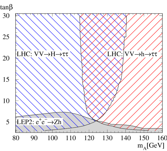
Figure F.2: $5\sigma$ discovery contours for $h\to\tau\tau$ and $H\to\tau\tau$ in WBF at the LHC, with $70$ fb^-1. An additional efficiency factor of 0.8 applied to the signal and all backgrounds due to pile-up is included beyond the first $30$ fb^-1. Also shown are the projected LEP2 exclusion limits (see text). Results are shown for SUSY parameters as in Fig. F.1, for maximal trilinear mixing, $A_{t}=\sqrt{6}M_{SUSY}$.

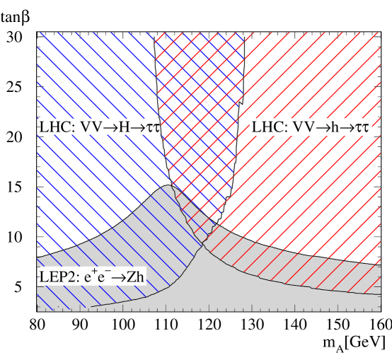
Figure F.3: Same as Fig. F.2, but for the case of no trilinear mixing, $A_{t}=0$.

Given the background rates determined in Ch. 5, which are of order 0.03 fb in a 20 GeV mass bin, except in the vicinity of the $Z$-peak, the expected significance of the $h/H\to\tau\tau$ signal can be determined. $5\sigma$ contours for an integrated luminosity of 70 fb^-1 are shown in Figs. F.2,F.3, as a function of $\tan\beta$ and $m_{A}$. I include an additional efficiency factor of 0.8 for both the signal and all backgrounds due to pile-up for data taken beyond the first $30$ fb^-1. Here the significances are determined from the Poisson probabilities of background fluctuations. Weak boson fusion, followed by decay to $\tau$-pairs, provides for a highly significant signal of at least one of the CP even Higgses. Even in the low $\tan\beta$ region, where LEP2 would discover the light Higgs, the WBF process at the LHC will give additional information. Most interesting is the transition region, where both $h$ and $H$ may be light enough to be observed via their $\tau\tau$ decay.

I have shown that the production of CP even MSSM Higgs bosons in WBF and subsequent decay to $\tau$ pairs gives a significant ($>5\sigma$) signal at the LHC. This search, with $\mathrel{\mathchoice{\lower 3.0pt\vbox{\halign{$\m@th\displaystyle\hfill{#}\hfil$\cr<\crcr\sim\crcr}}}{\lower 3.0pt\vbox{\halign{$\m@th\textstyle\hfill{#}\hfil$\cr<\crcr\sim\crcr}}}{\lower 3.0pt\vbox{\halign{$\m@th\scriptstyle\hfill{#}\hfil$\cr<\crcr\sim\crcr}}}{\lower 3.0pt\vbox{\halign{$\m@th\scriptscriptstyle\hfill{#}\hfil$\cr<\crcr\sim\crcr}}}}100$fb ^-1 of integrated luminosity, and supplemented by the search for $h/H\to\gamma\gamma$ in weak boson fusion, should cover the entire MSSM parameter space left after an unsuccessful LEP2 search, with a significant overlap of LEP2 and LHC search regions. The two CERN searches combined provide a no-lose strategy by themselves for seeing a MSSM Higgs. At the very least, the WBF measurements provide valuable additional information on Higgs couplings.

The present analysis relies only on the typical mixing behavior of the CP even mass eigenstates, and on the observability of a SM Higgs, of mass up to $\sim 150$ GeV, in WBF. This suggests that the search discussed here might also cover an extended Higgs sector as well as somewhat higher plateau masses, e.g. for very large squark soft-breaking mass parameters. Because decays into $\tau$ pairs are tied to the dominant decay channel of the intermediate mass range Higgs, $h/H\to\bar{b}b$, the search for a $\tau\tau$ signal in WBF is robust and expected to give a clear Higgs signal in a wide class of models.

References

- [1] C. Caso et al., Eur. Phys. J. C3, 1 (1998).
- [2] R.N. Cahn, Rev. Mod. Phys. 68, 951 (1996).
- [3] H. Georgi and S.L. Glashow, Phys. Rev. Lett. 32, 438 (1974); H. Georgi, H.R. Quinn and S. Weinberg, Phys. Rev. Lett. 33, 451 (1974).
- [4] T. Stelzer and W. F. Long, Comp. Phys. Comm. 81, 357 (1994), [hep-ph/9401258].
- [5] See e.g., O. Nachtmann, Elementary Particle Physics, Springer-Verlag (1990), Part II.
- [6] For a short course pedagodgical treatment of the Standard Model, see e.g., C. H. Llewellyn Smith, Proceedings of the 1989 Scottish Universities Summer School: Physics of the Early Universe, Edinburgh, Scotland (1989); P. Langacker, TASI lectures, QCD & Beyond: Proceedings, Theoretical Advanced Study Institute in Elementary Particle Physics, Boulder Colorado, 1995, edited by D. Soper, World Scientific (1996); or P.S. Drell, hep-ex/9701001.
- [7] F. Halzen and A.D. Martin, Quarks And Leptons: An Introductory Course In Modern Particle Physics, Wiley (1984), Ch. 15.
- [8] M.E. Peskin and D.V. Schroeder, An Introduction to quantum field theory, Addison Wesley (1995), Ch. 20.
- [9] V. I. Borodulin, R. N. Rogalev and S. R. Slabospitsky, hep-ph/9507456.
- [10] S. Willenbrock, hep-ph/9702330.
- [11] B. W. Lee, C. Quigg and H. B. Thacker, Phys. Rev. Lett. 38, 883 (1977); and Phys. Rev. D16, 1519 (1977).
- [12] C. Quigg, talk presented at the 27th International Meeting on Fundamental Physics, Granada, 1-5 Feb. 1999, hep-ph/9905369.
- [13] A. Djouadi, Acta Phys. Polon. B27, 3837 (1996).
- [14] V. Ruhlmann-Kleider, “New Particle Searches”, talk presented at Lepton-Photon ’99, Stanford University, 9-14 Aug. 1999.
- [15] See e.g., F. Halzen and A.D. Martin, Quarks And Leptons: An Introductory Course In Modern Particle Physics, Wiley (1984), Ch. 10; or M.E. Peskin and D.V. Schroeder, An Introduction to quantum field theory, Addison Wesley (1995), Ch. 17.
- [16] See e.g., T. Sjostrand, Proceedings of the 15th Brazilian National Meeting on Particles and Fields, Angra dos Reis, Brazil (1994).
- [17] T. Sjostrand, hep-ph/9508391.
- [18] G. Marchesini et al., hep-ph/9607393.
- [19] F. E. Paige, S. D. Proto pescu, H. Baer and X. Tata, hep-ph/9810440.
- [20] W.T. Giele, T. Matsuura, M.H. Seymour and B.R. Webber, contribution to Proceedings of the 1990 Summer Study on High Energy Physics: Research Directions for the Decade, Snowmass, CO (1990); W. Giele, private communication; T. Stelzer, private communication.
- [21] See e.g., F. Halzen and A.D. Martin, Quarks And Leptons: An Introductory Course In Modern Particle Physics, Wiley (1984), Ch. 4; or O. Nachtmann, Elementary Particle Physics, Springer-Verlag (1990), Ch. 5.
- [22] H. Murayama, I. Watanabe and K. Hagiwara, KEK-91-11.
- [23] For recent reviews, see e.g. S. Dawson, [hep-ph/9703387]; M. Spira, Fortsch. Phys. 46, 203 (1998); and references therein.
- [24] W. J. Marciano and F. E. Paige, Phys. Rev. Lett. 66, 2433 (1991); J. F. Gunion, Phys. Lett. B261, 510 (1991).
- [25] A. Stange, W. Marciano, and S. Willenbrock, Phys. Rev. D50, 4491 (1994), [hep-ph/9404247]; R. Kleiss, Z. Kunszt, W. J. Stirling, Phys. Lett. B253, 269 (1991); H. Baer, B. Bailey, J. F. Owens, Phys. Rev. D47, 2730 (1993).
- [26] R. N. Cahn, S.D. Ellis, R. Kleiss and W.J. Stirling, Phys. Rev. D35, 1626 (1987); V. Barger, T. Han, and R. J. N. Phillips, Phys. Rev. D37, 2005 (1988); R. Kleiss and W. J. Stirling, Phys. Lett. 200B, 193 (1988); D. Froideveaux, in Proceedings of the ECFA Large Hadron Collider Workshop, Aachen, Germany, 1990, edited by G. Jarlskog and D. Rein (CERN report 90-10, Geneva, Switzerland, 1990), Vol II, p. 444; M. H. Seymour, ibid, p. 557; U. Baur and E. W. N. Glover, Nucl. Phys. B347, 12 (1990); Phys. Lett. B252, 683 (1990).
- [27] V. Barger, K. Cheung, T. Han, and R. J. N. Phillips, Phys. Rev. D42, 3052 (1990); V. Barger et al., Phys. Rev. D44, 1426 (1991); V. Barger, K. Cheung, T. Han, and D. Zeppenfeld, Phys. Rev. D44, 2701 (1991); erratum Phys. Rev. D48, 5444 (1993); Phys. Rev. D48, 5433 (1993); V. Barger et al., Phys. Rev. D46, 2028 (1992).
- [28] D. Dicus, J. F. Gunion, and R. Vega, Phys. Lett. B258, 475 (1991); D. Dicus, J. F. Gunion, L. H. Orr, and R. Vega, Nucl. Phys. B377, 31 (1991).
- [29] V. Barger, M .S. Berger, A. L. Stange, and R. J. N. Phillips, Phys. Rev. D45, 4128 (1992).
- [30] T. Han, G. Valencia, and S. Willenbrock, Phys. Rev. Lett. 69, 3274 (1992).
- [31] Y. L. Dokshitzer, V. A. Khoze, and S. Troian, in Proceedings of the 6th International Conference on Physics in Collisions, (1986) ed. M. Derrick (World Scientific, 1987) p.365; J. D. Bjorken, Int. J. Mod. Phys. A7, 4189 (1992); Phys. Rev. D47, 101 (1993).
- [32] V. Barger, R. J. N. Phillips, and D. Zeppenfeld, Phys. Lett. B346, 106 (1995).
- [33] R. Cahn and S. Dawson, Phys. Lett. 136B, 196 (1984).
- [34] D. Rainwater and D. Zeppenfeld, Journal of High Energy Physics 12, 005 (1997).
- [35] D. Rainwater, D. Zeppenfeld and K. Hagiwara, Phys. Rev. D59, 014037 (1999).
- [36] D. Rainwater and D. Zeppenfeld, hep-ph/9906218.
- [37] D. Rainwater, R. Szalapski, and D. Zeppenfeld, Phys. Rev. D54, 6680 (1996), [hep-ph/9605444].
- [38] T. Han, G. Valencia and S. Willenbrock, Phys. Rev. Lett. 69, 3274 (1992).
- [39] V. Barger and R. J. N. Phillips, Phys. Rev. Lett. 55, 2752 (1985); H. Baer, V. Barger, H. Goldberg, and R. J. N. Phillips, Phys. Rev. D37, 3152 (1988).
- [40] For recent reviews, see e.g. J.L. Rosner, Comments Nucl. Part. Phys. 22, 205 (1998) [hep-ph/9704331]; K.Hagiwara, Ann. Rev. Nucl. Part. Sci. 1998, 463; W.J. Marciano, hep-ph/9902332; and references therein.
- [41] W. W. Armstrong et al., Atlas Technical Proposal, report CERN/LHCC/94-43 (1994); G. L. Bayatian et al., CMS Technical Proposal, report CERN/LHCC/94-38 (1994).
- [42] A. Djouadi, J. Kalinowski and M. Spira, Comput. Phys. Commun. 108, 56 (1998).
- [43] V. Barger, T. Han, J. Ohnemus and D. Zeppenfeld, Phys. Rev. D41, 2782 (1990).
- [44] F. Halzen, P. Hoyer, and W. J. Stirling, Phys. Lett. 188B, 375, 1987; M. Drees and T. Han, Phys. Rev. Lett. 77, 4142 (1996), [hep-ph/9605430].
- [45] S. Behrends and J. Lamoureux, FERMILAB-CONF-97-204-E (1997).
- [46] R. Kinnunen, private communication.
- [47] E.W. Glover, J. Ohnemus and S.S. Willenbrock, Phys. Rev. D37, 3193 (1988); V. Barger, G. Bhattacharya, T. Han and B.A. Kniehl, Phys. Rev. D43, 779 (1991).
- [48] M. Dittmar and H. Dreiner, Phys. Rev. D55, 167 (1997); and [hep-ph/9703401].
- [49] A. Stange, private communication.
- [50] A. Duff and D. Zeppenfeld, Phys. Rev. D50, 3204 (1994); K. Iordanidis and D. Zeppenfeld, Phys. Rev. D57, 3072 (1998), [hep-ph/9709506].
- [51] S. D. Ellis, R. Kleiss, and W. J. Stirling, Phys. Lett. 154B, 435 (1985); R. Kleiss and W. J. Stirling, Nucl. Phys. B262, 235 (1985); Phys. Lett. 180B, 171 (1986); J. F. Gunion, Z. Kunszt, and M. Soldate, Phys. Lett. 163B, 389 (1985); Erratum, Phys. Lett. 168B, 427 (1986); J. F. Gunion and M. Soldate, Phys. Rev. D34, 826 (1986); R. K. Ellis and R. J. Gonsalves, in Proc. of the Workshop on super high energy physics, Eugene, OR (1985), ed. D. E. Soper, p. 287.
- [52] K. Hagiwara and D. Zeppenfeld, Nucl. Phys. B313, 560 (1989).
- [53] V. Barger, T. Han and J. Ohnemus, and D. Zeppenfeld, Phys. Rev. Lett. 62, 1971 (1989); Phys. Rev. D40, 2888 (1989).
- [54] F. A. Berends et al., Phys. Lett. B224, 237 (1989).
- [55] H. Chehime and D. Zeppenfeld, Phys. Rev. D47, 3898 (1993).
- [56] D. Rainwater, T. Plehn, and D. Zeppenfeld, in preparation.
- [57] D. Rainwater, D. Summers, and D. Zeppenfeld, Phys. Rev. D55, 5681 (1997).
- [58] K. Hagiwara, A. D. Martin, and D. Zeppenfeld, Phys. Lett. B235, 198 (1990).
- [59] D. Cavalli et al., ATLAS Internal Note PHYS-NO-051, Dec. 1994.
- [60] E. Richter-Was et al., Int. J. Mod. Phys. A13, 1371 (1998).
- [61] F. A. Berends, H. Kuijf, B. Tausk, and W. T. Giele, Nucl. Phys. B357, 32 (1991).
- [62] V. Barger, E. Mirkes, R. J. N. Phillips, and T. J. Stelzer, Phys. Lett. B338, 336 (1994).
- [63] R. K. Ellis et al., Nucl. Phys. B297, 221 (1988).
- [64] B. K. Bullock, K. Hagiwara, and A. D. Martin, Phys. Lett. B273, 501 (1991); Nucl. Phys. B395, 499 (1993).
- [65] H. L. Lai et al., Phys. Rev. D55, 1280 (1997), [hep-ph/9606399].
- [66] D. Cavalli, L. Cozzi, L. Perini, S. Resconi, ATLAS Internal Note PHYS-NO-051, Dec. 1994.
- [67] G.P. Lepage, CLNS-80/447.
- [68] T. Ishikawa et al., KEK-92-19.
- [69] E.E. Boos et al., hep-ph/9503280.
- [70] See e.g., Z. Kunszt and F. Zwirner, Nucl. Phys. B385, 3 (1992); E. Richter–Was et al., Int. J. Mod. Phys. A13, 1371 (1998); M. Spira, Fortschr. Phys. 46, 203 (1998); and references therein.
- [71] T. Plehn, D. Rainwater and D. Zeppenfeld, Phys. Lett. B454, 297 (1999).
- [72] See e.g. J.F. Gunion and A. Turski, Phys. Rev. D39, 2701 (1989).
- [73] H. E. Haber and R. Hempfling, Phys. Rev. D48, 4280 (1993); M. Carena, J. R. Espinosa, M. Quiros, and C. E. M. Wagner, Phys. Lett. B355, 209 (1995).
- [74] S. Heinemeyer, W. Hollik and G. Weiglein, Phys. Rev. D58, 091701 (1998); R.-J. Zhang, Phys. Lett. B447, 89 (1999).
- [75] See Reports of the Working Groups, Physics at Run II – Supersymmetry/Higgs, Batavia, 1998.
- [76] See Talks by the LEP Collaborations, LEPC 11/12/98.
- [77] J.F. Gunion and H.E. Haber, Nucl. Phys. B272, 1 (1986); erratum ibid B402, 567 (1993).
- [78] T. Plehn, D. Rainwater and D. Zeppenfeld, Phys. Lett. B454, 297 (1999).