Implementing quadratic supergravity inflation

Abstract

We study inflation driven by a slow-rolling inflaton field, characterised by a quadratic potential, and incorporating radiative corrections within the context of supergravity. In this model the energy scale of inflation is not overly constrained by the requirement of generating the observed level of density fluctuations and can have a physically interesting value, e.g. the supersymmetry breaking scale of $10^{10}$ GeV or the electroweak scale of $10^{3}$ GeV. In this mass range the inflaton is light enough to be confined at the origin by thermal effects, naturally generating the initial conditions for a (last) stage of inflation of the new inflationary type.

I Introduction

The modern paradigm for cosmological inflation is generically termed ‘chaotic’, referring primarily to its choice of initial conditions [1]. In its simplest form, a single scalar field — the inflaton $\phi$ — evolves slowly along its potential $V(\phi)$ towards its minimum at the origin. The essential challenge is to embed consistently this potential in an underlying particle physics model, within a natural range of variation of the parameters involved and respecting the ‘slow-roll conditions’ [2]. These are upper limits on the normalized slope and curvature of the potential:

$$\epsilon\equiv\frac{M^{2}}{2}\left(\frac{V^{\prime}}{V}\right)^{2}\ll 1,\qquad|\eta|\equiv M^{2}\left|\frac{V^{\prime\prime}}{V}\right|\ll 1.$$ (1)

Here $M\,(\equiv\,M_{\rm P}/\sqrt{8\pi}\simeq 2.44\times 10^{18}{\rm GeV})$ is the normalised Planck mass and the potential determines the Hubble parameter during inflation as, $H_{\rm inf}\equiv\dot{a}/a\simeq\sqrt{V/3M^{2}}$. Inflation ends (i.e. $\ddot{a}$, the acceleration of the cosmological scale factor, changes sign from negative to positive) when $\epsilon$ and/or $|\eta|$ become of ${\cal O}(1)$.

It is easy to see that this challenge is not met by simple models of the potential. Consider the quadratic form [3]

$$V(\phi)=\frac{1}{2}m_{\phi}^{2}\phi^{2}.$$ (2)

The adiabatic scalar density perturbation generated through quantum fluctuations of the inflaton is [2]

$$\delta^{2}_{\rm H}(k)=\frac{1}{150\pi^{2}}\frac{V_{\rm H}}{M^{4}}\frac{1}{\epsilon_{\rm H}}\ ,$$ (3)

where the subscript ${\rm H}$ denotes the epoch at which a fluctuation of wavenumber $k$ crosses the Hubble radius $H^{-1}$ during inflation, i.e. when $aH=k$. (We normalise $a=1$ at the present epoch, when the Hubble expansion rate is $H_{0}\equiv 100h$ km s^-1Mpc^-1, with $h\sim 0.5-0.8$.) The COBE observations [4] of anisotropy in the cosmic microwave background on large angular-scales require [2]

$$\delta_{\rm COBE}\simeq 1.9\times 10^{-5},$$ (4)

on the scale of the observable universe ($k_{\rm COBE}^{-1}\sim\,H_{0}^{-1}\sim 3000h^{-1}$ Mpc). In addition, the COBE data fix the spectral index, $n_{\rm H}(k)\equiv 1+{\rm d}\delta_{\rm H}^{2}(k)/{\rm d}\ln\,k=1-6\epsilon_{\rm H}+2\eta_{\rm H}$, on this scale:

$$n_{\rm COBE}=1.2\pm 0.3.$$ (5)

The slow-roll condition (1) together with the COBE normalisation (4) then implies

$$\langle\phi\rangle\gg M,\quad m_{\phi}\ll H_{\rm inf}\ll 10^{15}{\rm GeV},$$ (6)

at the epoch when the fluctuations observed by COBE were generated. Similarly if we consider the quartic potential $V=\frac{1}{4}\lambda\phi^{4}$ [3], eqs.(1) and (4) imply

$$\langle\phi\rangle\gg M,\qquad\lambda\ll 10^{-11}.$$ (7)

Thus we see that the slow-roll condition (especially on $\eta$) generically requires $\langle\phi\rangle\gg\,M$ which is difficult to motivate in a particle physics model. In models incorporating gravity, non-renormalisable corrections of the form $(\langle\phi\rangle/M)^{n}$ are unsuppressed at large $\langle\phi\rangle$ for any $n$ and do not have the monomial form usually assumed in chaotic inflationary models. Furthermore the COBE measurement of the scalar perturbation amplitude implies extreme fine tuning because the only natural scale for $m_{\phi}$ is the Planck scale $M$, in conflict with eq.(6). Alternatively an extremely small value is required for the self-coupling as in eq.(7), which also represents unnatural fine tuning.

Given the difficulty of constructing realistic particle physics models which can drive inflation for large $\langle\phi\rangle$, it is natural to ask whether there are viable models which work for small $\langle\phi\rangle$, i.e. ‘new inflation’ [5] in which the potential has a maximum at the origin and the inflaton evolves away from it. In this case low powers of $\langle\phi\rangle/M$ will dominate the potential during the era of observable inflation. Starting from $\langle\phi\rangle\sim 0$ and assuming that the symmetry properties of the model forbid a linear term, the quadratic term will dominate, giving a potential of the form

$$V(\phi)\sim\Delta^{4}-\frac{1}{2}m_{\phi}^{2}\phi^{2}+\dots,$$ (8)

where the constant vacuum energy $\Delta^{4}$ is now the leading term in the potential. From eq.(1) we have now the constraint

$$m_{\phi}\ll H_{\rm inf}\sim\Delta^{2}/M,$$ (9)

and this is again much smaller than the natural value for the mass. To solve this problem we are driven to consider theories in which a symmetry prevents $m_{\phi}$ from being large. The only known symmetry capable of achieving this is supersymmetry which can guarantee that $m_{\phi}$ vanishes in the limit that supersymmetry is unbroken. However the non-vanishing potential of eq.(8) driving inflation breaks (global) supersymmetry and so, even in supersymmetric models, $m_{\phi}$ will be non-zero in general. In the extreme case that the inflaton has vanishing non-gravitational couplings, gravitational effects will typically induce a mass of order $H_{\rm inf}\sim\Delta^{2}/M$ for any scalar field [6], in particular the inflaton [7]. Nevertheless this is a big improvement over the non-supersymmetric case, for the fine tuning problem now simply becomes one of requiring $m_{\phi}=\beta\Delta^{2}/M$ with $\beta\lesssim 0.1$ to obtain successful inflation.

In this Letter we summarise the results of a general analysis of supergravity inflationary models in which a quadratic term dominates the evolution of the potential for small values of the inflaton. As discussed in Section II, one can find models for which $\beta$ is naturally small, consistent with the slow-roll requirements. However, even in these models it is difficult to make the mass negligibly small so that the quadratic term is likely to be dominant at small inflaton field values. For this reason we consider models of inflation driven by a quadratic term to be the most natural supersymmetric inflationary models. However such models still leave unanswered several important questions concerning the initial conditions.

The most important question is why the universe should initially be homogeneous enough for slow-roll inflation to begin [1]. In chaotic models [3], inflation begins when the scale of the potential energy is of order the Planck scale and the horizon (the scale over which the universe must be homogeneous for inflation to start) is also of order the Planck scale. By contrast in the models discussed here, inflation starts much later when the horizon contains many such Planck scale horizons and, in this case, it is difficult to understand how the necessary level of homogeneity can be realised. However this argument is not really a criticism of the possibility that there be a late stage of inflation but rather a statement that this cannot be all there is. Thus we are implicitly assuming that there was some other process which ensured the necessary homogeneity at the begining of quadratic inflation, as in the original chaotic inflation scenario [3] or in the context of quantum cosmology [8]. Such models lead to a situation in which a homogeneous universe emerges at the Planck era and potential energy is released reheating the universe and possibly setting the conditions for further periods of inflation to occur.

This leads to the second initial condition question, namely why should such a universe subsequently undergo inflation at a lower energy scale? In the case of interest here this amounts to asking why the inflaton field has initially such a small value that slow-roll inflation from the neighbourhood of the origin is possible? Remarkably, within the context of supersymmetric inflationary models there is a straightforward answer because quite generally supersymmetry is broken by finite temperature effects i.e. the inflaton potential at high temperatures is not likely to be the same as that at zero temperature

$$V(\phi,T)\left|{}_{\min}\neq V(\phi,0)\right|_{\min}$$ (10)

As we discuss later, thermal effects may readily drive the inflaton to the origin where the symmetry is enhanced, thus offering an elegant solution to this initial condition problem. Of course this requires that the system be initially in thermal equilibrium and this is not normally the case in slow-roll inflationary models, particularly since the inflaton should be very weakly coupled in order not to spoil the required flatness of its potential. However quadratic inflation is special in as much as the value of the potential during inflation is not strongly constrained by the need to generate the correct magnitude of density fluctuations. For the case that the potential energy driving inflation is low, we will show that the processes leading to thermal equilibrium have time to work before the inflationary era starts.

A further possible advantage of lowering the inflationary scale is that it may be then readily identified with a scale already present in particle physics. For example a low $\Delta$ may be identified with the SUSY breaking scale in the hidden sector, $\Delta_{\rm SUSY}\sim 10^{10}{\rm GeV}$. As is well known [10] this yields a gravitino mass,

$$m_{3/2}\sim\frac{\Delta_{\rm SUSY}^{2}}{M}\sim 10^{2}{\rm GeV},$$ (11)

of order the electroweak scale, as is needed to avoid the hierarchy problem of Grand Unified Theories. Recently an even more radical solution to the hierarchy problem has been suggested, namely that the only fundamental scale is the electroweak breaking scale itself and that the (four dimensional) Planck scale is a derived quantity [9]. As we shall see, slow-roll quadratic inflation is possible even at the electroweak scale. In the next Section we discuss the expectation for the inflaton potential following from supergravity. Readers primarily interested in the cosmological implications may wish to skip this and go straight to Section III.

II The Supergravity potential

In $N=1$ supersymmetric theories with a single SUSY generator, complex scalar fields are the lowest components, $\phi^{a}$, of chiral superfields, $\Phi^{a}$, which contain chiral fermions, $\psi^{a}$, as their other components. In what follows we will take $\Phi^{a}$ to be left-handed chiral superfields so that $\psi^{a}$ are left-handed massless fermions. Masses for fields will be generated by spontaneous symmetry breakdown so that the only fundamental mass scale is the normalised Planck scale. This is aesthetically attractive and is also what follows if the underlying theory generating the effective low-energy supergravity theory emerges from the superstring. The $N=1$ supergravity theory describing the interaction of the chiral superfields is specified by the Kähler potential [10],

$$G(\Phi,\Phi^{\dagger})=d(\Phi,\Phi^{\dagger})+\ln|f(\Phi)|^{2}.$$ (12)

Here $d$ and $f$ (the superpotential) are two functions which need to be specified; they must be chosen to be invariant under the symmetries of the theory. The dimension of $d$ is 2 and that of $f$ is 3, so terms bilinear (trilinear) in the superfields appear without any mass factors in $d$ ($f$). The scalar potential following from eq.(12) is given by [10]

$$V=\exp\left(\frac{d}{M^{2}}\right)\left[F^{A\dagger}(d_{A}^{B})^{-1}F_{B}-3\frac{|f|^{2}}{M^{2}}\right]+{\rm D-terms},$$ (13)

where

$$F_{A}\equiv\frac{\partial f}{\partial\Phi^{A}}+\left(\frac{\partial d}{\partial\Phi^{A}}\right)\frac{f}{M^{2}},\qquad\left(d_{A}^{B}\right)^{-1}\equiv\left(\frac{\partial^{2}d}{\partial\Phi^{A}\partial\Phi_{B}^{\dagger}}\right)^{-1}.$$ (14)

At any point in the space of scalar fields $\Phi$ we can make a combination of a Kähler transformation and a holomorphic field redefinition such that $\phi^{a}=0$ at that point and the Kähler potential takes the form $d=\sum_{a}|\Phi_{a}|^{2}+\ldots$. In this form, the scalar kinetic terms are canonical at $\phi^{a}=0$ and from eq.(13), neglecting D-terms and simplifying to the case of a single scalar field, the scalar potential writes

$$V=\left({\rm e}^{|\phi|^{2}/M^{2}+\dots}\right)\left[|(f_{\phi}+f\phi^{\ast}+\dots)(1+\dots)|^{2}-3\frac{|f|^{2}}{M^{2}}\right]=V_{0}+|\phi|^{2}\frac{V_{0}}{M^{2}}+\dots$$ (15)

where $V_{0}\equiv\,V|_{\phi=0}$. Since inflation is driven by the non-zero value of $V$, we see that the resultant breaking of supersymmetry gives all scalar fields a contribution to their mass-squared of $V_{0}/M^{2}$, in conflict with the slow-roll condition (1) on $\eta$. This is the essential problem one must solve if one is to implement inflation in a supergravity theory. However, as stressed earlier, the problem is relatively mild when compared to the non-supersymmetric case because the suppression for $\eta$ need only be by a factor of 10 or so.

A Solving the $\eta$ problem

There have been several proposals for dealing with this problem. One widely explored possibility is D-term inflation [13]. In particular one may consider an anomalous D-term in eq.(13) of the form

$$\frac{g^{2}}{2}(\xi-\sum_{i}q_{i}|\widetilde{\phi}_{i}|^{2})^{2},$$ (16)

where $\xi$ is a constant and $\widetilde{\phi}_{i}$ are scalar fields charged under the anomalous $U(1)$ with charge $q_{i}$. Such a term, for vanishing $\widetilde{\phi}_{i}$, gives a constant term in the potential but does not contribute in leading order to the masses of uncharged scalar fields. The latter occur in radiative order only giving a contribution to their mass-squared equal to $\beta^{2}\,V_{0}/M^{2}$ where $\beta^{2}\approx\,h^{\prime 2}/16\pi^{2}$, and typically $\beta\approx 10^{-1}$ for an effective coupling $h^{\prime}\sim 1$ between the charged and neutral fields.

The other suggested ways out of the $\eta$ problem do not require non-zero D-terms during inflation but rather provide reasons why the quadratic term in eq.(15) should be anomalously small. One possibility follows from the fact that the mass term of ${\cal O}(V_{0}/M^{2})$ coming from eq.(15) actually applies at the Planck scale. Since we are considering inflation for field values near the origin the inflaton mass must be run down to low scales. As shown in ref.[16], in a wide class of models in which the gauge couplings become large at the Planck scale the low energy supersymmetry breaking soft masses are driven much smaller at low scales by radiative corrections. The typical effect is to reduce the mass by a factor $\beta\approx\alpha(M)/\alpha(\mu)$ where $\alpha(\mu)$ is a gauge coupling evaluated at the scale $\mu$. While radiative corrections can cause a significant change in the coupling, the effect is limited and becomes smaller as the gauge coupling becomes small. For this reason the effective mass at low scales cannot be arbitrarily small and typically $\beta\gtrsim 1/25$.

It is also possible to construct models in which the contribution to the scalar mass exhibited in eq.(15) is cancelled by further contributions coming from the expansion of $f$ in eq.(13). One interesting example which arises in specific superstring theories was discussed in ref.[14]. Another occurs in supergravity models of the ‘no-scale’ type [15]. In these examples, while the scalar mass is absent in leading order, it typically arises in radiative order and so again there is an expectation that the effective mass cannot be arbitrarily small.

To summarise, in all these cases for small field values the effective supergravity potential can be conveniently parameterised as a constant term plus a quadratic term involving a real inflaton field $\overline{\phi}$ (the real part of $\phi$) i.e. just the form of eq.(8). However this is the form at tree level only. In general radiative corrections cause the effective mass, $m_{\overline{\phi}}$ to depend logarithmically on $\overline{\phi}$. Thus the full potential has the form

$$V(\overline{\phi})=\Delta^{4}\left[1+b\left(\frac{|\overline{\phi}|}{M}\right)^{2}+c\ln\left(\frac{|\overline{\phi}|}{M}\right)\left(\frac{|\overline{\phi}|}{M}\right)^{2}\right].$$ (17)

Note that in eq.(17) we have not included a term linear in $\overline{\phi}$. Such a term can be forbidden if the theory has a symmetry under which $\overline{\phi}$ transforms non-trivially and we assume that this is indeed the case.

B Terminating slow-roll evolution

The form of eq.(17) provides a useful parameterisation of the inflationary potential in the neighbourhood of the origin. However when $\overline{\phi}/M$ is large higher order terms may be significant and so it is important to determine their structure. Such terms may occur through higher order terms in $d$ or $f$ in eq.(12) or in higher order terms in the expansion of eq.(15). Typically these terms are expected be associated with new physics at the Planck scale, for example a term in the superpotential of the form $\phi^{p/2+1}/M^{p/2-2}$ will give rise to terms of the form $|\phi|^{p}/M^{p-4}$ in the scalar potential. However it may happen that such higher order terms arise as a result of integrating out heavy fields in the theory, in which case the mass scale in the denominator can be much smaller than $M$. For example the superpotential $f=\phi^{2}X+M_{X}X^{2}$ describes a field $X$ with mass $M_{X}$. At scales below $M_{X}$ the field $X$ may be integrated out to give the effective superpotential $f=\phi^{4}/M_{X}$ in which the scale of the higher dimension operator is set by $M_{X}$. This mass may be associated with any of the scales in the theory, e.g. the inflationary scale or the supersymmetry breaking scale, and can thus be much smaller than the Planck scale.

With this preamble we now consider the structure of the terms responsible for ending inflation Consider first the inflationary models driven by a non-zero F-term. This is conveniently parameterised by the superpotential $f=\Delta^{2}Y$ which gives $V=|F_{Y}|^{2}=\Delta^{4}$ as required. Radiative corrections then lead to the form of eq.(17). Now consider the form of higher order corrections to this superpotential. The terms allowed must be consistent with any gauge or discrete symmetries of the models. For example the above form linear in $Y$ follows if $Y$ carries non-zero $R$-symmetry charge under an unbroken $R$-symmetry. Using such symmetries it is straightforward to construct a general potential displaying the possibilities for ending inflation. We suppose that $\phi$ is a singlet under the $R$-symmetry but carries a charge under a discrete $Z_{p}$ symmetry. Then the superpotential has the form

$$f=\left(\Delta^{2}-\frac{\phi^{p}}{M^{\prime p-2}}-\frac{\phi^{2p}}{M^{\prime 2p-2}}-\dots\right)Y$$ (18)

where we have suppressed the coefficients of ${\cal O}(1)$ of each term. This gives rise to the potential

$$V=\left(\Delta^{2}-\frac{\phi^{p}}{M^{\prime p-2}}-\frac{\phi^{2p}}{M^{\prime 2p-2}}-\dots\right)^{2},$$ (19)

plus terms involving $Y$ which we drop as they do not contribute to the vacuum energy (since $Y$ does not acquire a vacuum expectation value). This has the desired structure for ending inflation because the potential vanishes for $\phi\sim\,M^{\prime}(\Delta/M^{\prime})^{2/p}$ for $M^{\prime}>\Delta$. For our analysis we use a slightly simplified form of eq.(19) (c.f. eq.(30)) keeping only the leading $\phi^{p}$ term and setting $M^{\prime p-2}=\Delta^{q}M^{p-q-2}$ to take account of the possibility discussed above that the scale associated with the higher dimension operators may be below the Planck scale.

The situation is similar for the case of $D$-term inflation. From eq.(16) we see there is a contribution of the form of eq.(19). If $\widetilde{\phi_{i}}$ is a heavy field it may be integrated out in a similar manner to that discussed above so that the term $\sum_{i}q_{i}|\widetilde{\phi}_{i}|^{2}$ may give rise to a higher dimension term of the form $\phi^{p}/M^{\prime p-2}.$ Thus the parameterisation of eq.(30) may apply to this case as well.

III Quadratic supergravity inflation

We wish to study locally supersymmetric slow-roll inflationary models in which the inflaton field evolves from small to large field values. Near the origin the term involving the lowest power of the inflaton field is the most important in the potential, hence a simple parameterisation is adequate. As discussed above, we may take the inflaton field, $\overline{\phi}$, to be real with a quadratic potential of the form (17). It is convenient to work with dimensionless quantities

$$\tilde{V}(\tilde{\phi})\equiv\frac{V(\overline{\phi}/M)}{\Delta^{4}}\ ,\qquad\tilde{\phi}\equiv\frac{\overline{\phi}}{M}\ ,\qquad\tilde{\Delta}\equiv\frac{\Delta}{M}\ ,$$ (20)

in terms of which the potential and its derivatives are given by

$$\tilde{V}(\tilde{\phi}) = 1+b\tilde{\phi}^{2}+c\tilde{\phi}^{2}\ln\tilde{\phi}^{2},$$ (21)

$$\tilde{V}^{\prime}(\tilde{\phi}) = 2\tilde{\phi}(b+c+c\ln\tilde{\phi}^{2}),$$ (22)

$$\tilde{V}^{\prime\prime}(\tilde{\phi}) = 2(b+3c+c\ln\tilde{\phi}^{2}).$$ (23)

During slow-roll inflation with $\tilde{\phi}\ll 1$, one has

$$\tilde{V}(\tilde{\phi})\approx 1,\qquad\epsilon\ll|\eta|,$$ (24)

hence at $\tilde{\phi}=\tilde{\phi}_{\rm H}$, the spectrum of the scalar perturbations (3) can be written as

$$\delta_{\rm H}\simeq\pm\frac{2\tilde{\Delta}^{2}}{\sqrt{75}\pi(1-n_{\rm H}+8c)\tilde{\phi}_{\rm H}}\ ,$$ (25)

where the spectral index is

$$n_{\rm H}\simeq 1+2\tilde{V}^{\prime\prime}(\tilde{\phi}_{\rm H})=1+4b+12c+8c\ln\tilde{\phi}_{\rm H}.$$ (26)

The $+(-)$ sign in eq.(25) takes into account that $\tilde{V}^{\prime}$ is positive (negative) at $\tilde{\phi}=\tilde{\phi}_{\rm H}$ corresponding to the inflaton rolling towards smaller (bigger) values of $\tilde{\phi}$. We focus on the latter case as it offers a simple way of ending inflation as the field value increases and higher order terms in $\tilde{\phi}$ become important.

The number of e-folds before the end of inflation when the fluctuations observed by COBE were generated is

$$N_{\rm COBE}\simeq 48+\ln\left(\frac{\Delta}{10^{10}{\rm GeV}}\right),$$ (27)

assuming instant reheating; the numerical value would be smaller if reheating is inefficient or if there are later episodes of ‘thermal inflation’ [2]. In our model the end of inflation occurs due to terms of higher order in $\phi$ of the form given in eq.(19). For the moment we parameterise their effect through the inclusion of a further parameter $\phi_{\rm e}$, the value of the field at the end of inflation. The number of e-folds from $\phi_{\rm H}$ onwards should equal or exceed $N_{\rm COBE}$, giving

$$N_{\rm H}\equiv-\int_{\tilde{\phi}_{\rm H}}^{\tilde{\phi}_{\rm e}}\frac{V(\tilde{\phi})}{V^{\prime}(\tilde{\phi})}{\rm d}\tilde{\phi}=\frac{1}{4c}\ln\left(\frac{b+c+2c\ln\tilde{\phi}_{\rm H}}{b+c+2c\ln\tilde{\phi}_{\rm e}}\right)\geq N_{{\rm COBE}}.$$ (28)

In addition the slow-roll conditions during inflation require

$$|V^{\prime\prime}(\tilde{\phi})|\ll\gamma,\quad{\rm for}\quad\tilde{\phi}_{\rm H}<\tilde{\phi}<\tilde{\phi}_{\rm e},$$ (29)

where $\gamma$ is of ${\cal O}(1)$ (and can be calculated exactly in the slow-roll formalism).

If eqs.(25, 26, 28) satisfy the observational constraints (4,5, 27) the inflationary era will lead to a satisfactory cosmology. For $b\lesssim 25c$ the term proportional to $b$ in eq.(17) is negligible. We shall concentrate on this limit (although acceptable inflation is also possible if this is not the case). Then eq.(26) constrains the quantity $\frac{1}{c}\ln[\ln(\tilde{\phi}_{H})/\ln(\tilde{\phi}_{e})]$. Further, eq.(25) constrains a combination of $\tilde{\Delta}$, $c$, and $\tilde{\phi}_{\rm H}$. Given that we have four parameters to satisfy these equations and that eq.(29) can be satisfied for a range of parameters, we see that acceptable inflation follows for a range of $\Delta$. This opens up the possibility of having a much lower value for the inflationary energy scale than is usually considered. The value of $\Delta$ is very sensitive to the the value of $\tilde{\phi}_{e}$ and so it is necessary to consider in some detail what determines the latter. We will discuss this shortly but first we consider how a reduction in the scale of inflation, $\Delta$, may allow thermal effects to naturally set the initial conditions for inflation.

A The begining of inflation

We assume that some process at the Planck scale, presumably quantum cosmological in nature [8], creates a homogeneous patch of space-time and releases energy thermalising the universe. It is important to note that the thermalisation temperature cannot be close to the Planck scale, regardless of the amount of energy released, essentially because particle interactions are asymptotically free. For example, an explicit calculation of the $q\bar{q}$ annihilation rate into gluons finds that equilibrium can only be attained below a temperature $T_{\rm therm}\sim 3\times 10^{14}$ GeV [11].

Let us consider the requirements on the inflaton field for it to be localised at the origin through its couplings to particles in the thermal bath. On dimensional grounds, the $2\to 2$ scattering/annihilation cross-sections at energies higher than the masses of the particles involved are expected to decrease with increasing temperature as $\sim\alpha^{2}/T^{2}$, where $\alpha$ is the coupling. Thus if the scattering/annihilation rate, $\Gamma\sim\,n\langle\sigma\,v\rangle$ is to exceed the Hubble expansion rate $H_{\rm therm}\sim(g_{*}T^{4}/10M^{2})^{1/2}$ in the radiation-dominated plasma, then we have a limit on the thermalisation temperature $T_{\rm therm}\lesssim\alpha^{2}M/3g_{*}^{1/2}$, where $g_{*}$ counts the relativistic degrees of freedom (=915/4 in the minimal supersymmetric standard model (MSSM) at high temperatures). Now a Yukawa coupling $h^{\prime}\phi\chi^{2}$ of the inflaton to MSSM fields $\chi$ will generate a confining potential at high temperatures, $V(\phi,T)\sim\,h^{\prime 2}T^{2}\phi^{2}$ i.e. an effective mass for the inflaton of $m_{\rm therm}\sim\,h^{\prime}T$. This will rapidly drive the inflaton field to the origin in a time of ${\cal O}(m_{\rm therm}^{-1})$ As the universe cools, the potential energy $\sim\Delta^{4}$ of the inflaton will begin to dominate over the thermal energy at a temperature $T_{\rm inf}\sim\Delta^{2}/\alpha^{2}M$. At this epoch the inflaton field will be localised to a region $\delta\phi\sim\,T_{\rm inf}$ in the neighbourhood of the origin. Thus to provide natural initial conditions for new inflation we require that $T_{\rm inf}<T_{\rm therm}$ i.e. that the scale of inflation be sufficiently low. The discussion above yields the constraint $\Delta\lesssim 10^{-4}M$, taking $\alpha\sim 1/24$.

B The end of inflation

As mentioned earlier, the end of inflation will be determined by terms which are not included in the expansion of the inflationary potential keeping only terms up to quadratic order. In general such terms are quite model dependent as all orders in $\phi$ may contribute significantly for large $\phi$. However it is necessary to discuss the expectation for $\phi_{\rm e}$ for reasonable forms of the potential since the nature of the inflationary era is strongly dependent on it. In Section II we have discussed how higher order terms arise in supergravity theories and how they are restricted by the symmetries of the theory but here we will simply write down the structure of these terms motivated by such considerations. Although this parameterisation involves only a single inflaton field in the present context , it actually covers a wide range of models including hybrid inflationary models in which the end of inflation is triggered by a second field. The full inflationary potential then has the form:

$$V(\phi)=\left(1-\kappa\frac{\tilde{\phi}^{p}}{\Delta^{q}}\right)^{2}+b\tilde{\phi}^{2}+c\tilde{\phi}^{2}\ln\tilde{\phi}^{2},$$ (30)

where $\kappa$ is a coupling which for simplicity we set to unity (its most natural value?) in our calculations.

The end of slow-roll occurs at

$$\tilde{\phi}_{\rm e}=\left(\frac{\gamma\Delta^{q}}{2\kappa p(p-1)}\right)^{1/(p-2)}.$$ (31)

Using this we may now determine the range of parameters for which acceptable inflation obtains by identifying $\tilde{\phi}_{\rm H}$ with the field value at which the fluctuations observed by COBE were generated. In Figure 1 we show the required inflationary scale for various values of $p,q$, setting $\gamma,\kappa=1$ and adopting $c=b/25$. The essential observation is that the quadratic potential generates acceptable inflation for a wide range of values of $\Delta$. This is important because it opens up the possibility of identifying the inflationary scale with a mass scale already required in the particle physics model. Further if $\Delta\lesssim 10^{14}{\rm GeV}$, thermal effects will be important in setting the initial conditions for inflation. For the cases shown in Figure 1, inflation typically ends at $\tilde{\phi}_{\rm e}\sim 10^{-8}$ and the fluctuations observed by COBE exited the Hubble radius at $\tilde{\phi}_{\rm COBE}\sim 10^{-11}-10^{-9}$, about 50 e-folds of expansion earlier. We have checked that in all cases $\tilde{\phi}_{\rm COBE}$ exceeds $T_{\rm inf}$ so that there will be sufficient inflation starting with thermal initial conditions.

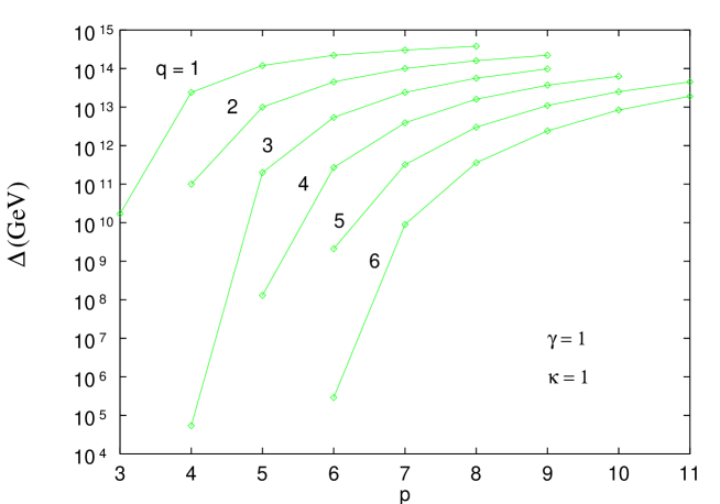
FIG. 1.: The inflationary energy scale for various choices of the non-renormalisable term which terminates inflation.

IV Conclusions

We have studied in very general terms, an inflationary era driven by a quadratic potential. The essential requirement for successful inflation is that the inflaton mass be reduced below the Hubble parameter. We have discussed mechanisms which do this, concentrating on the situation where the inflaton mass-squared is negative at the origin. This has the advantage that thermal initial conditions naturally place the inflaton at the origin, initiating the inflationary era. Whether such inflation occurs is a model dependent question. In compactified string theories the multiplet structure is completely determined and typically there are many scalar fields with the properties of the inflaton discussed here. In such models inflation driven by a quadratic potential is a very natural possibility.

In order for the above mechanism to work, the inflaton must couple to the fields in the thermal bath and the scale of its potential must be sufficiently low. In fact the quadratic parametrization of the inflationary potential allows any value for the inflationary scale $\Delta$. This is essentially because the end of inflation occurs not due to the violation of the slow-roll conditions by the quadratic potential, but due to higher order non-renormalisable terms which become important as the inflaton evolves towards large field values. Two values for the inflationary scale are of particular interest and will be discussed in detail elsewhere [19]. One has $\Delta\sim 10^{10}~{}{\rm GeV}$, the supersymmetry breaking scale in the hidden sector. The other with $\Delta\sim 10^{3}~{}{\rm GeV}$ implements inflation at the electroweak scale and could be relevant in the context of theories with submillimeter dimensions.

REFERENCES

- [1] see, A.D. Linde, Particle Physics and Inflationary Cosmology (Harwood Academic Press, 1990).
- [2] For a review and extensive references, see, D.H. Lyth and A. Riotto, Phys. Rep. 314 (1999) 1.
- [3] A.D. Linde, Phys. Lett. 129B (1983) 177.
- [4] C.L. Bennett et al (COBE collab.), Astrophys. J. 464 (1996) L1.
- [5] A.D. Linde, Phys. Lett. 108B (1982) 389; A. Albrecht and P.J. Steinhardt, Phys. Rev. Lett. 48 (1982) 1220.
- [6] M. Dine, W. Fischler and D. Nemechansky, Phys. Lett. 136B (1984) 169; G. Coughlan, W. Fischler, E.W. Kolb, S. Raby and G.G. Ross, Phys. Lett. 140B (1984) 44.
- [7] E. Copeland, A.R. Liddle, D.H. Lyth, E.D. Stewart and D. Wands, Phys. Rev. D49 (1994) 6410.
- [8] S.W. Hawking and N. Turok, Phys. Lett. B425 (1998) 25; A. Vilenkin, Phys. Rev. D57 (1998) 7069; A.D. Linde, Phys. Rev. D58 (1998) 083514 N. Turok and S.W. Hawking, Phys. Lett. B432 (1998) 271.
- [9] N. Arkani-Hamed, S. Dimopoulos and G. Dvali, Phys. Lett. B429 (1998) 263.
- [10] D. Bailin and A. Love, Supersymmetric Gauge Field Theory and String Theory (Adam Hilger, 1994).
- [11] K. Enqvist and J. Sirkka, Phys. Lett. B314 (1993) 298;
- [12] K. Enqvist and K.J. Eskola, Mod. Phys. Lett. A5 (1990) 1919.
- [13] E.D. Stewart, Phys. Rev. D51 (1995) 6847; E. Halyo, Phys. Lett. B387 (1996) 43; P. Binétruy and G. Dvali, Phys. Lett. B388 (1996) 241; for a review and further references, see [2].
- [14] J.A. Casas and G.B. Gelmini, Phys. Lett. B410 (1997) 36.
- [15] M.K. Gaillard, H. Murayama and K.A. Olive, Phys. Lett. B355 (1995) 71; M. Bastero-Gil and S.F. King, Nucl.Phys. B549 (1999) 391.
- [16] S.F. King and G.G. Ross, Nucl. Phys. B530 (1998) 3.
- [17] E.D. Stewart, Phys. Rev. D56 (1997) 2019.
- [18] E.D. Stewart, Phys. Lett. B391 (1997) 34; L. Covi, D.H. Lyth and L. Roszkowski, Phys. Rev. D60 (1999) 023509; L. Covi and D.H. Lyth, Phys. Rev. D60 (1999) 063515
- [19] G. Germán, G.G. Ross and S. Sarkar, in preparation.