Padé-Summation Approach to QCD $\beta$-Function Infrared Properties

Abstract

In view of the successful asymptotic Padé-approximant predictions for higher-loop terms within QCD and massive scalar field theory, we address whether Padé-summations of the $\overline{MS}$ QCD $\beta$-function for a given number of flavours exhibit an infrared-stable fixed point, or alternatively, an infrared attractor of a double valued couplant as noted by Kogan and Shifman for the case of supersymmetric gluodynamics. Below an approximant-dependent flavour threshold $(6\leq n_{f}\leq 8)$, we find that Padé-summation $\beta$-functions incorporating $[2|1],[1|2],[2|2],[1|3]$, and $[3|1]$ approximants whose Maclaurin expansions match known higher-than-one-loop contributions to the $\beta$-function series always exhibit a positive pole prior to the occurrence of their first positive zero, precluding any identification of this first positive zero as an infrared-stable fixed point of the $\beta$- function. This result is shown to be true regardless of the magnitude of the presently-unknown five-loop $\beta$-function contribution explicitly appearing within Padé-summation $\beta$-functions incorporating $[2|2],[1|3]$, and $[3|1]$ approximants. Moreover, the pole in question suggests the occurrence of dynamics in which both a strong and an asymptotically-free phase share a common infrared attractor. We briefly discuss the possible relevance of infrared-attractor dynamics to the success of recent calculations of the glueball mass spectra in QCD with $N_{c}\rightarrow\infty$ via supergravity. As $n_{f}$ increases above an approximant-dependent flavour threshold, Padé-summation $\beta$-functions incorporating $[2|2],[1|3]$, and $[3|1]$ approximants exhibit dynamics controlled by an infrared-stable fixed point over a widening domain of the five-loop $\overline{MS}$ $\beta$-function parameter $(\beta_{4}/\beta_{0})$. Subsequent to the above-mentioned flavour threshold, all approximants considered exhibit infrared-stable fixed points that decrease in magnitude with increasing flavour number.

1 Introduction

Asymptotic Padé-approximant methods have been utilized to estimate higher order contributions to renormalization-group (RG) functions within both QCD [1, 2, 3] and massive scalar field theory [2, 3, 4], for which such estimates compare quite favourably with explicit calculation [5]. More recently, such methods have been shown to predict RG-accessible coefficients of logarithms within five-loop-order contributions to QCD correlation functions with striking accuracy [6]. These results are all derived from an improvement of Padé-estimated coefficients which incorporates the estimated error of Padé-approximants in predicting the $n!K^{-n}n^{\gamma}$ asymptotic behaviour expected for $n^{th}$ order coefficients of a field-theoretic perturbative series [7, 8]. For $[N|M]$ approximants, such error is seen to decrease with increasing N and M [1, 2, 7], as well as to favour diagonal and near-diagonal approximants [9].

Of course, the use of such higher approximants becomes tenable only if the corresponding perturbative series is known to sufficiently high order. A known series of the form $\sum_{j=1}^{k}R_{j}x^{j}$ specifies all coefficients within $[N|M]$-approximants to the series only for $\{N,M\}$ such that $k=N+M$; even four-loop calculations (corresponding to $k=3$ if the leading $x^{2}$ behaviour is factored out from the series) serve only to specify $[2|1]$, $[1|2]$, and $[0|3]$ approximants. Nevertheless, such approximants have been used in conjunction with the anticipated asymptotic error to predict the next (five-loop) coefficient $R_{4}$ as well as the corresponding diagonal $[2|2]$ approximant to the full field-theoretic series.[1, 2, 3, 4, 6]

The success of such predictions for those cases in which $R_{4}$ is known [1, 3, 6] suggests that

1. Padé approximants determined from $\{R_{1},...,R_{k}\}$ more accurately represent the field-theoretic asymptotic series $\sum_{j=0}R_{j}x^{j}$ than mere truncation of this series to $\sum_{j=0}^{k}R_{j}x^{j}$;

2. Sufficiently-high Padé-approximants grow arbitrarily close to the function of $x$ represented by the full field-theoretic series, as suggested by asymptotic error formulae [1] following from renormalon-estimates of large-$j$ coefficients in the series [7].

In the absence of alternatives other than explicit series truncation, such “Padé-summation” [1, 2] of the full perturbative series may provide a much wanted means for extrapolating such series to the infrared region. We are particularly interested in two possible scenarios for infrared dynamics within QCD, either the infrared attractor suggested by Kogan and Shifman within the context of supersymmetric gluodynamics [10], or alternatively, dynamics governed by an infrared-stable fixed point. In reference [2], for example, a Padé-summation of the $n_{f}=3$ QCD $\beta$-function is argued to contain a zero corresponding to an infrared fixed point comparable to that predicted by Mattingly and Stevenson [11, 12].

Indeed it is this claim that provides some of the motivation for our present work. In the approach of ref. [12], an infrared-stable fixed point is argued to occur even when $n_{f}=0$, in contradiction to a broadening consensus that values of $n_{f}$ even larger than 3 are required for infrared-stable fixed points to occur [13, 14, 15, 16, 17]; e.g. $n_{f}=8$ is suggested by a two-loop truncation of the QCD $\beta$-function, with consequences for the phase-structure of QCD first explored by Banks and Zaks [18].

In the present paper, we utilize the perturbative series for the $\overline{MS}$ QCD $\beta$-function, now known in full to four-loop order [19], in order to construct $[N|M]$ Padé summations, which are assumed to provide information about the $\beta$-function’s first positive zero or pole (this point is further discussed in Section 2). We are able to extend our analysis past $N+M=3$ by expressing $N+M=4$ approximants in terms of the presently-unknown five-loop $\beta$ function coefficient, which is treated here as a variable parameter. Among the specific issues we address in the sections that follow are:

1. the existence of a flavour-threshold for dynamics governed by an infrared stable-fixed point,

2. whether differing Padé-approximants are consistent in predicting infrared properties of QCD,

3. the dependence of Padé-predictions for $\beta$-function infrared properties on the presently-unknown five-loop term,

4. the size of the infrared fixed point, particularly in comparison with the $\alpha_{s}^{*}=\pi/4$ benchmark value for chiral-symmetry breaking [13, 14],

5. the existence of a strong phase of QCD for $n_{f}=0$ [10] and, possibly, for nonzero $n_{f}$ as well, and

6. the elevation of the true infrared cutoff (mass gap) of $n_{f}=3$ QCD to hadronic mass scales (500 - 700 MeV).

In Section 2, we discuss how Padé-approximants constructed from the known terms of the $\beta$-function series can exhibit information about the infrared behaviour of the corresponding couplant. This approach relies upon the Padé-approximant remaining closer to the true $\beta$-function than the truncated perturbation series from which the approximant is constructed, as discussed above. We conclude Section 2 by obtaining Padé-summation expressions for QCD $\overline{MS}$ $\beta$-functions which incorporate $[2|1]$, $[1|2]$, $[2|2]$, $[1|3]$ and $[3|1]$ approximants to post-one-loop terms in the $\beta$-function series. The latter three approximants are expressed in terms of a variable $R_{4}(\equiv\beta_{4}/\beta_{0})$ characterizing the presently unknown 5-loop contribution to the $\overline{MS}$ $\beta$-function.

In Section 3, we apply such Padé-summation methods to the $\beta$-function characterizing $N_{c}=3\;QCD$ with no fundamental fermions. Padé-summation predictions for the infrared structure of $n_{f}=0$ QCD in the ’t Hooft ($N_{c}\rightarrow\infty$) limit [20] are presented separately in an Appendix. For both cases, we find that no Padé-summation $\beta$-function supports the existence of an infrared-stable fixed point for the $n_{f}=0$ QCD couplant. Moreover, we demonstrate that the infrared behaviour extracted from Padé- summations of the $n_{f}=0$ QCD $\beta$-function appears to be governed by an apparent $\beta$-function pole, an infrared-attractor of two ultraviolet phases of the couplant. This behaviour is in qualitative agreement with that extracted from supersymmetric QCD in the absence of fundamental-representation matter fields [10]. We conclude Section 3 with a brief discussion of the possible applicability of infrared-attractor dynamics to the glueball spectrum for the $N_{c}\rightarrow\infty$ case.

In Section 4, we extend the analysis of Section 3 to nonzero $n_{f}$. Specifically, we examine Padé-summation $\beta$-functions which incorporate $[2|1]$, $[1|2]$, $[2|2]$, $[1|3]$ and $[3|1]$ approximants to post-one-loop terms in the perturbative $\beta$-function series. We find that all such approximants exhibit a flavour threshold for the occurrence of infrared dynamics characterized by an infrared-stable fixed point. Beneath this threshold, which occurs between 6 and 9 flavours (depending on the approximant), no infrared-stable fixed point is possible regardless of the magnitude of the unknown five-loop term ($\beta_{4}$) entering such approximants. Above the threshold, we observe a progressively broadening domain of $\beta_{4}/\beta_{0}$ for which an infrared-stable fixed point occurs, as well as a decrease in the magnitude of such fixed points with increasing $n_{f}$.

In Section 5, we focus on the infrared behaviour of the $n_{f}=3$ case. We show that $[2|2]$, $[1|3]$ and $[3|1]$ Padé-summations of the $n_{f}=3$ perturbative $\beta$-function series yield similar infrared dynamics to the “gluodynamic” $n_{f}=0$ case of Section 3. Such summations are all shown to yield an enhanced mass gap, an infrared boundary to the domain of $\alpha_{s}$ somewhat in excess of 500 MeV, regardless of the 5-loop contribution to the $\beta$-function series. This infrared boundary is shown to be remarkably stable against such 5-loop corrections to the $\beta$-function.

2 Methodology

2.1 A Toy $\beta$-Function:

Padé-approximants to a function whose Maclaurin series is $1+\sum_{k=1}R_{k}x^{k}$ are well known to be valid for a broader range of the expansion parameter $x$ than truncations of the series. Consider, for example, the following toy $\beta$-function

$$\mu^{2}\frac{dx}{d\mu^{2}}=\beta_{A}(x)\equiv-x^{2}[sec(x)-tan(x)]$$ (2.1)

We have chosen $\beta_{A}$ to be asymptotically free, i.e., to have an ultraviolet fixed point at $x=0$. Since

$$\lim_{x\rightarrow\pi/2}\left(sec(x)-tan(x)\right)=0$$ (2.2)

we have also chosen $\beta_{A}$ to have an infrared fixed point at $x=\pi/2$. $\beta_{A}$ has a subsequent pole at $x=3\pi/2$, and $\beta_{A}$ alternates zeros and poles as $x$ increases by subsequent increments of $\pi$. The point here, however, is that the solution to (2.1) will exhibit the same dynamics as depicted in Fig. 1 for $x$ between zero and $\pi/2$, corresponding to a freezing-out of the coupling at the $x=\pi/2$ infrared-stable fixed point.

Suppose, however, that the sum-total of our knowledge of $\beta_{A}$ is the first five-terms of this series expansion, corresponding to a hypothetical five-loop $\beta$-function calculation:

$$\beta_{A}^{(5)}(x)=-x^{2}\left[1-x+\frac{x^{2}}{2}-\frac{x^{3}}{3}+\frac{5x^{4}}{24}\right]$$ (2.3)

This truncated series is, of course, not equal to zero at the $x=\pi/2$ infrared fixed point. Rather, when $x=\pi/2$, each term in the series is seen to be comparable to prior lower-order terms:

$$\beta_{A}^{(5)}(\pi/2)=-\frac{\pi^{2}}{4}\left[1-1.571+1.233-1.292+1.269\right]$$ (2.4)

One would necessarily conclude that the field theoretical calculation leading to (2.3) cannot be extended to large enough $x$ to extract information about the infrared properties of $\beta_{A}(x)$.

The series (2.3), however, provides sufficient information to construct a $[2|2]$ approximant to the degree-four polynomial within (2.3):

$$\beta_{A}^{[2|2]}(x)=-x^{2}\left[\frac{1-\frac{x}{2}-\frac{x^{2}}{12}}{1+\frac{x}{2}-\frac{x^{2}}{12}}\right]$$ (2.5)

Equation (2.5) is obtained by requiring that the degree-2 numerator and denominator polynomials of the $[2|2]$ approximant be chosen so as to yield a Maclaurin expansion whose first five terms reproduce the five terms in (2.3). One can easily verify that $\beta_{A}^{[2|2]}$ remains closer to $\beta_{A}$ (2.1) over a much larger range of $x$ than $\beta_{A}^{(5)}$, as given in (2.3). This range is inclusive of the first zero of $\beta_{A}$. $\beta_{A}^{[2|2]}$ has a positive zero at $x=1.583$, quite close to $\beta_{A}$’s true zero at $\pi/2$. Moreover, the denominator in (2.5) remains positive over the entire range $0\leq x\leq 1.583$, guaranteeing that $x=1.583$ is infrared-stable (a sign change would render this fixed-point ultraviolet-stable). Thus, Padé-improvement of the information in (2.3) provides a means for extracting information about the infrared properties of $\beta_{A}$ that is otherwise inaccessible from the “five-loop” expression.

2.2 $\beta$-Function Poles

It should also be noted that (2.5) predicts that a pole at $x=7.58$ follows the zero at 1.583 without a second intervening zero. This result is qualitatively similar to the true behaviour of $\beta_{A}$, which acquires a pole at $x=3\pi/2$ subsequent to the zero at $\pi/2$ without any additional intervening zeros. However, accuracy in predicting this pole, as well as any subsequent zeros or poles, is clearly beyond the scope of (2.5), the $[2|2]$ Padé-summation of $\beta_{A}$.

We have seen, however, that Padé methods do provide a window for viewing leading $\beta$-function singularities that would otherwise be inaccessible. One cannot automatically dismiss the possibility of such singularities occurring within QCD $\beta$-functions. For example, the $\beta$-function of $SU(N_{c})$ SUSY gluodynamics, which is known exactly if no matter fields are present, exhibits precisely such a zero [21]:

$$\beta(x)=-\frac{3N_{c}x^{2}}{4}\left[\frac{1}{1-N_{c}x/2}\right];\;\;x\equiv\frac{\alpha_{s}}{\pi}.$$ (2.6)

Eq. (2.6), which can be derived via imposition of the Adler-Bardeen theorem upon the supermultiplet of the anomalies [22], implies the existence of a strong ultraviolet phase (the upper branch of Fig. 2) when the couplant $x$ is greater than the $\beta$-function pole at $2/N_{c}$ [10]. Interestingly, the $\beta$-function (2.6) is itself a $[0|1]$ approximant once the leading $-3N_{c}x^{2}/4$ coefficient is factored out.

To demonstrate how Padé summation provides a window for extracting possible pole singularities in true $\beta$-functions, we consider a second toy example

$$\mu^{2}\frac{dx}{d\mu^{2}}\equiv\beta_{B}(x)=x^{2}\left[sec(x)+tan(x)\right].$$ (2.7)

$\beta_{B}(x)$ is asymptotically free, but has a positive pole at $x=\pi/2$ prior to its first zero at $x=3\pi/2$. This zero is an ultraviolet stable fixed point because of the overall sign change associated with passing through the pole at $x=\pi/2$. The behaviour of $x(\mu)$ for $x<3\pi/2$ is schematically depicted in Fig 2, with $x=\pi/2$ corresponding to $\mu_{c}$, the minimum allowed value of $\mu$ (assuming the couplant $x$ is real).

Such infrared structure is not at all evident in the “five-loop” approximation to (2.7)

$$\beta_{B}^{(5)}(x)=-x^{2}\left[1+x+\frac{x^{2}}{2}+\frac{x^{3}}{3}+\frac{5x^{4}}{24}\right],$$ (2.8)

an expression which ceases to be close to the true $\beta$-function (2.7) for values of $x$ substantially smaller than $x=\pi/2$. However, one can obtain a $[2|2]$ approximant directly from the truncated series in (2.8)

$$\beta_{B}^{[2|2]}(x)=-x^{2}\frac{[1+\frac{x}{2}-\frac{x^{2}}{12}]}{[1-\frac{x}{2}-\frac{x^{2}}{12}]}$$ (2.9)

whose Maclaurin expansion yields (2.8) for its first five terms. The first denominator zero of (2.9) is at $x=1.583$, in good agreement with the positive pole of (2.7) at $x=\pi/2$. Moreover, the first denominator zero of (2.9) precedes all (positive) numerator zeros, thereby eliminating the possibility of the pole being preceded by an infrared fixed point. Thus, (2.9) and the true $\beta$-function (2.7) predict very similar dynamics between the ultraviolet-stable fixed point at $x=0$ and the infrared-attractor pole at $x=\pi/2$. By contrast, the “five-loop” $\beta$-function (2.8) can only reproduce the true running couplant in the ultraviolet region where $x$ is near zero.

2.3 Padé-Improvement and Infrared Behaviour

It is to be emphasized that the examples presented above demonstrate how Padé-improvement may provide information about the infrared region that a truncated perturbative series cannot. There is no way, of course, to prove that the first positive zero or pole of a given Padé-summation is indeed the first zero or pole of the true $\beta$-function. In the absence of methodological alternatives, however, we will explore below the consequences of assuming this to be the case. Corroboration of such an assumption relies ultimately on an explicit comparison of next-order terms calculated for the $\overline{MS}$ QCD $\beta$-function series, to Padé-predictions for these terms (e.g., ref [3]). There is reason to be encouraged, however, by the success already demonstrated for Padé predictions of the known five-loop content of the massive scalar field theory $\beta$-function [1, 4]. Similar successes are obtained in predicting RG-accessible coefficients within the five loop contributions to QCD vector and scalar fermionic-current correlation functions, as well as within four-loop contributions to the scalar gluonic-current correlation function [3, 6].

The general approach we take is to replace a $k$-loop truncation of the asymptotic $\beta$-function series

$$\beta^{(k)}(x)=-\beta_{0}x^{2}\left(1+R_{1}x+...R_{k-1}x^{k-1}\right)$$ (2.10)

with an expression incorporating the corresponding $[N|M]$ Padé- approximant $(N+M=k-1)$:

$$\beta^{[N|M]}(x)=-\beta_{0}x^{2}\left(\frac{1+a_{1}x+...+a_{N}x^{N}}{1+b_{1}x+...+b_{M}x^{M}}\right)$$ (2.11)

The $N+M$ coefficients $\{a_{1},...,a_{N},b_{1},...,b_{M}\}$ are completely determined by the requirement that the first $k$ terms in the Maclaurin expansion of (2.11) replicate $\beta^{(k)}(x)$ (2.10). We then examine $\beta^{[N|M]}$ in order to determine whether or not it is supportive of an infrared-stable fixed point, as in Fig. 1, or an infrared-attractor pole, as in Fig. 2.

If the first positive zero of the degree-N polynomial in the numerator of (2.11) precedes any positive zeros of the degree-M polynomial in the denominator, that first numerator zero corresponds to the infrared-stable fixed point at which the couplant $x$ freezes out in Fig. 1. Alternatively, if the first positive zero in the denominator of (2.11) precedes any positive zeros in the degree-M numerator polynomial, that first denominator zero corresponds to the infrared-attractor pole common to both couplant phases of Fig. 2.

2.4 A Padé Roadmap

It will prove useful to tabulate those formulae required to obtain Padé approximants (2.11) whose Maclaurin expansions reproduce the truncated series (2.10) for the $\overline{MS}$ $\beta$-function. Values for $\beta_{0}$, $R_{1}$, $R_{2}$ and $R_{3}$ for the $\beta$-function, as defined by (2.10), are tabulated in Table 1. Corresponding $[2|1]$ and $[1|2]$ approximants to the truncated series $1+R_{1}x+R_{2}x^{2}+R_{3}x^{3}$ within (2.10) are given by the following formulae:

$n_{f}$	$\beta_{0}$	$R_{1}$	$R_{2}$	$R_{3}$
0	11/4	51/22	2857/352	41.5383
1	31/12	67/31	62365/8928	34.3295
2	29/12	115/58	48241/8352	27.4505
3	9/4	16/9	3863/864	20.9902
4	25/12	77/50	21943/7200	15.0660
5	23/12	29/23	9769/6624	9.83592
6	7/4	13/14	-65/224	5.51849
7	19/12	10/19	-12629/5472	2.42409
8	17/12	1/34	-22853/4896	1.00918
9	5/4	-3/5	-1201/160	1.97366
10	13/12	-37/26	-41351/3744	6.44815
11	11/12	-28/11	-49625/3168	16.3855
12	3/4	-25/6	-6361/288	35.4746
13	7/12	-47/7	-64223/2016	71.6199
14	5/12	-113/10	-70547/1440	145.373
15	1/4	-22	-2823/32	332.091
16	1/12	-151/2	-81245/288	1309.98

Table 1: The known coefficients $\beta_{0}$ and $R_{1,2,3}$ appearing in the QCD $\beta$-function (2.10) for $n_{f}=0-16$, as calculated in [19].

$$\beta^{[2|1]}(x)=-\beta_{0}x^{2}\left[\frac{1+a_{1}x+a_{2}x^{2}}{1+b_{1}x}\right],$$ (2.12a)

$$a_{1}=(R_{1}R_{2}-R_{3})/R_{2},$$ (2.12b)

$$a_{2}=(R_{2}^{2}-R_{1}R_{3})/R_{2},$$ (2.12c)

$$b_{1}=-R_{3}/R_{2},$$ (2.12d)

and

$$\beta^{[1|2]}(x)=-\beta_{0}x^{2}\left[\frac{1+a_{1}x}{1+b_{1}x+b_{2}x^{2}}\right],$$ (2.13a)

$$b_{1}=(R_{3}-R_{1}R_{2})/(R_{1}^{2}-R_{2}),$$ (2.13b)

$$b_{2}=(R_{2}^{2}-R_{1}R_{3})/(R_{1}^{2}-R_{2}),$$ (2.13c)

$$a_{1}=R_{1}+b_{1}.$$ (2.13d)

We do not consider the $[0|3]$-approximant, as this approximant has no possible numerator zeros and therefore cannot lead to an infrared fixed point. The $[3|0]$-approximant is, of course, the truncated series itself. The “diagonal-straddling” $[1|2]$ and $[2|1]$ approximants are the only $N+M=3$ approximants for which both infrared-stable fixed points (Fig. 1) and infrared-attractor poles (Fig. 2) are possible, depending on the specific ordering of positive numerator and denominator zeros in (2.12a) and (2.13a). Hence, it is these approximants we will study in subsequent sections.

$R_{4}$, the “next-order” coefficient of the QCD $\beta$-function (2.10), is not presently known. Nevertheless, one can construct “diagonal-straddling” $[2|2]$, $[1|3]$ and $[3|1]$ approximants with $R_{4}$ taken to be an arbitrary parameter, by utilizing the values for $\{R_{1},R_{2},R_{3}\}$ given in Table 1. One finds for the truncated series $\beta^{(5)}(x)$ $=-\beta_{0}x^{2}\left[1+R_{1}x+R_{2}x^{2}+R_{3}x^{3}+R_{4}x^{4}\right]$ the following Padé-approximant $\beta$-functions:

$$\beta^{[2|2]}(x)=-\beta_{0}x^{2}\left[\frac{1+a_{1}x+a_{2}x^{2}}{1+b_{1}x+b_{2}x^{2}}\right],$$ (2.14a)

$$b_{1}=(R_{1}R_{4}-R_{2}R_{3})/(R_{2}^{2}-R_{1}R_{3}),$$ (2.14b)

$$b_{2}=(R_{3}^{2}-R_{2}R_{4})/(R_{2}^{2}-R_{1}R_{3}),$$ (2.14c)

$$a_{1}=R_{1}+b_{1},$$ (2.14d)

$$a_{2}=R_{1}b_{1}+b_{2}+R_{2};$$ (2.14e)

$$\beta^{[1|3]}(x)=-\beta_{0}x^{2}\left[\frac{1+a_{1}x}{1+b_{1}x+b_{2}x^{2}+b_{3}x^{3}}\right]$$ (2.15a)

$$b_{1}=\frac{(R_{1}^{2}R_{2}-R_{2}^{2}-R_{1}R_{3}+R_{4})}{(2R_{1}R_{2}-R_{1}^{3}-R_{3})},$$ (2.15b)

$$b_{2}=\frac{(R_{1}^{2}R_{3}-R_{1}R_{2}^{2}+R_{2}R_{3}-R_{4}R_{1})}{2R_{1}R_{2}-R_{1}^{3}-R_{3}},$$ (2.15c)

$$b_{3}=\frac{[R_{3}^{2}+R_{2}^{3}-2R_{1}R_{2}R_{3}+R_{4}(R_{1}^{2}-R_{2})]}{2R_{1}R_{2}-R_{1}^{3}-R_{3}}$$ (2.15d)

$$a_{1}=R_{1}+b_{1};$$ (2.15e)

$$\beta^{[3|1]}(x)=-\beta_{0}x^{2}\left[\frac{1+a_{1}x+a_{2}x^{2}+a_{3}x^{3}}{1+b_{1}x}\right],$$ (2.16a)

$$a_{1}=R_{1}-R_{4}/R_{3},$$ (2.16b)

$$a_{2}=R_{2}-R_{1}R_{4}/R_{3},$$ (2.16c)

$$a_{3}=R_{3}-R_{2}R_{4}/R_{3},$$ (2.16d)

$$b_{1}=-R_{4}/R_{3}.$$ (2.16e)

Given the known values of $\{R_{1},R_{2},R_{3}\}$ tabulated in Table 1, we have tabulated $\beta^{[2|2]}$’s coefficients $\{a_{1},a_{2},b_{1},b_{2}\}$ in Table 2 for all $n_{f}$-values for which $x=0$ is an ultraviolet-stable fixed point. These coefficients are all linear in the unknown parameter $R_{4}$. A similar tabulation of the coefficients within $\beta^{[1|3]}$ and $\beta^{[3|1]}$ is presented in Tables 3 and 4, respectively. Because all such Padé-coefficients are $R_{4}$-dependent for a given choice of $n_{f}$, one might expect to find infrared stable fixed point behaviour (Fig. 1) for some range of $R_{4}$, infrared-attractor pole behaviour (Fig. 2) for another range of $R_{4}$, and (possibly) some regimes of $R_{4}$ for which there are neither numerator nor denominator zeros. Surprisingly, we find in Section 4 that infrared-stable fixed point behaviour as in Fig. 1 does not occur for any of the diagonal-straddling approximants (2.12-15) until $n_{f}$ reaches a threshold value, regardless of $R_{4}$. This threshold depends on the approximant considered, but is greater than or equal to 6 for all $[N|M]$ approximants discussed above.

$n_{f}$	$a_{1}$	$a_{2}$	$b_{1}$	$b_{2}$
0	13.4026-0.0762155 $R_{4}$	-22.9153+0.0901663$R_{4}$	-0.0762155$R_{4}$ + 11.0844	0.266848$R_{4}$ - 56.7275
1	116019-0.0850858$R_{4}$	-19.0068+0.0911037$R_{4}$	-0.0850858$R_{4}$+9.44058	0.274999$R_{4}$-46.3959
2	9.50934-0.0941220$R_{4}$	-15.0709+0.0875660$R_{4}$	-0.0941220$R_{4}$+7.52659	0.274187$R_{4}$-35.7703
3	7.19456-0.102610$R_{4}$	-11.3292+0.0756438$R_{4}$	-0.102610$R_{4}$ + 5.41678	0.258062$R_{4}$-25.4301
4	4.84008-0.110684$R_{4}$	-8.18415+0.0485887$R_{4}$	-0.110684$R_{4}$+3.30008	0.219042$R_{4}$-16.3139
5	2.67929-0.123291$R_{4}$	-6.19674-0.0112453$R_{4}$	-0.123291$R_{4}$+1.41842	0.144208$R_{4}$ - 9.45997
6	0.610851-0.184236$R_{4}$	-6.62748-0.228650$R_{4}$	-0.184236$R_{4}$-0.317721	-0.0575739$R_{4}$-6.04228
7	1.907466+0.129932$R_{4}$	-0.130346+0.638145$R_{4}$	0.1299318$R_{4}$+1.38115	0.569760$R_{4}$+1.45066
8	0.245912+0.00135179$R_{4}$	-4.61451+0.214571$R_{4}$	0.00135179$R_{4}$+0.216500	0.214531$R_{4}$+0.0468084
9	-0.342477-0.0104297$R_{4}$	-7.59305+0.136738$R_{4}$	-0.0104297$R_{4}$+0.257228	0.130480$R_{4}$+0.0677118
10	-0.880095-0.0108500$R_{4}$	-11.5003+0.099648$R_{4}$	-0.0184997$R_{4}$+0.542982	0.0842074$R_{4}$+0.317008
11	-1.65139 - 0.00886659$R_{4}$	-17.0050+0.0771335$R_{4}$	-0.00886659$R_{4}$ + 0.894061	0.0545640$R_{4}$ + 0.935218
12	-2.93401-0.00655509$R_{4}$	-25.2430+0.0620604$R_{4}$	-0.00655509$R_{4}$+1.23265	0.0347475$R_{4}$+1.97982
13	-5.18889-0.00448899$R_{4}$	-38.6692+0.0514389$R_{4}$	-0.00448899$R_{4}$+1.52540	0.0212985$R_{4}$+3.42939
14	-9.53837-0.00279507$R_{4}$	-63.6700+0.0437023$R_{4}$	-0.00279507$R_{4}$+1.76163	0.0121180$R_{4}$+5.22737
15	-20.0584-0.00145806$R_{4}$	-123.626+0.0379240$R_{4}$	-0.00145806$R_{4}$+1.94165	0.00584673$R_{4}$+7.30916
16	-73.4295-0.000423006$R_{4}$	-428.807+0.0335175$R_{4}$	-0.000423006$R_{4}$ + 2.07047	0.00158053$R_{4}$+9.61460

Table 2: Coefficients $a_{1,2}$ and $b_{1,2}$ of $\beta^{[2|2]}$, the $[2|2]$ Padé-approximant (2.13) to the QCD $\beta$ function for $n_{f}=0-16$. The coefficients are all linear in $R_{4}$, the (presently-) unknown five-loop term in (2.10).

$n_{f}$	$a_{1}$	$b_{1}$	$b_{2}$	$b_{3}$
0	9.56239-0.0611053$R_{4}$	7.24421-0.0611053$R_{4}$	-24.9099+0.141653$R_{4}$	-42.5901+0.167582$R_{4}$
1	8.51104-0.0702708$R_{4}$	6.34975-0.0702708$R_{4}$	-20.7090+0.151876$R_{4}$	-33.9265+0.162617$R_{4}$
2	7.25658-0.0810329$R_{4}$	5.27382-0.0810329$R_{4}$	-16.2327+0.160669$R_{4}$	-25.7265+0.149477$R_{4}$
3	5.80845-0.0933552$R_{4}$	4.03067-0.0933552$R_{4}$	-11.6367+0.165965$R_{4}$	-18.3242+0.122349$R_{4}$
4	4.24716-0.107164$R_{4}$	2.70716-0.107164$R_{4}$	-7.21667+0.165032$R_{4}$	-12.2028+0.07244688$R_{4}$
5	2.76704-0.123131$R_{4}$	1.50617-0.123131$R_{4}$	-3.37387+0.155253$R_{4}$	-7.80319-0.0141605$R_{4}$
6	1.72453-0.145814$R_{4}$	0.795958-0.145814$R_{4}$	-0.448926+0.135399$R_{4}$	-4.87066-0.168040$R_{4}$
7	1.97486-0.200029$R_{4}$	1.44855-0.200029$R_{4}$	1.54554+0.105278$R_{4}$	0.105614-0.517062$R_{4}$
8	17.0270-0.778954$R_{4}$	16.9976-0.7789537917$R_{4}$	4.16776+0.0229104$R_{4}$	78.2076-3.63659$R_{4}$
9	-8.58112+0.137934$R_{4}$	-7.98112+0.137934$R_{4}$	2.71758+0.0827604$R_{4}$	-60.2514+1.08502$R_{4}$
10	-6.27351+0.0358829$R_{4}$	-4.85044+0.0358829$R_{4}$	4.14206+0.0510641$R_{4}$	-54.12482+0.468980$R_{4}$
11	-6.36697+0.0125229$R_{4}$	-3.82151+0.0125229$R_{4}$	5.93697+0.0318765$R_{4}$	-61.1352+0.277305$R_{4}$
12	-7.44146+0.00452652$R_{4}$	-3.27479+0.00452652$R_{4}$	8.44183+0.0188605$R_{4}$	-72.6300+0.178562$R_{4}$
13	-9.70448+0.00151777$R_{4}$	-2.99019+0.00151777$R_{4}$	11.7796+0.010191$R_{4}$	-87.7855+0.116775$R_{4}$
14	-14.2164+0.000415849$R_{4}$	-2.91637+0.000415849$R_{4}$	16.0360+0.00469909$R_{4}$	-107.043+0.0734726$R_{4}$
15	-25.0410+7.04348$\cdot$10-5$R_{4}$	-3.04098+7.04348$\cdot$10-5$R_{4}$	21.3172+0.00154956$R_{4}$	-131.384+0.0403041$R_{4}$
16	-78.8684+2.12019$\cdot$10-6$R_{4}$	-3.36839+2.12019$\cdot$10-6$R_{4}$	27.7873+0.000160074$R_{4}$	-162.269+0.0126837$R_{4}$

Table 3: Coefficients $a_{1}$ and $b_{1,2,3}$ of $\beta^{[1|3]}$, the $[1|3]$ Padé-approximant (2.14) to the QCD $\beta$-function for $n_{f}=0-16$. $R_{4}$ is the unknown five-loop contribution to the $\beta$-function.

$n_{f}$	$a_{1}$	$a_{2}$	$a_{3}$	$b_{1}$
0	2.31818-0.0240742$R_{4}$	8.11648-0.0558083$R_{4}$	41.5383-0.195397$R_{4}$	-0.0240742$R_{4}$
1	2.16129-0.0291294$R_{4}$	6.98533-0.0629572$R_{4}$	34.3295-0.203479$R_{4}$	-0.0291294$R_{4}$
2	1.98276-0.0364292$R_{4}$	5.77598-0.0722302$R_{4}$	27.4505-0.210414$R_{4}$	-0.0364292$R_{4}$
3	1.77778-0.0476412$R_{4}$	4.47106-0.0846954$R_{4}$	20.9902-0.213007$R_{4}$	-0.0476412$R_{4}$
4	1.54000-0.0663747$R_{4}$	3.04764-0.102217$R_{4}$	15.0650-0.202286$R_{4}$	-0.0663747$R_{4}$
5	1.26087-0.101668$R_{4}$	1.47479-0.128190$R_{4}$	9.83592-0.149939$R_{4}$	-0.101668$R_{4}$
6	0.928571-0.181209$R_{4}$	-0.290179-0.168265$R_{4}$	5.51849+0.0525830$R_{4}$	-0.181209$R_{4}$
7	0.526316-0.412526$R_{4}$	-2.30793-0.217119$R_{4}$	2.42409+0.952081$R_{4}$	-0.412526$R_{4}$
8	0.0294118-0.990906$R_{4}$	-4.66769-0.0291443$R_{4}$	1.00918+4.62524$R_{4}$	-0.990906$R_{4}$
9	-0.600000-0.506673$R_{4}$	-7.50625+0.304004$R_{4}$	1.97366+3.80322$R_{4}$	-0.506673$R_{4}$
10	-1.42308-0.155083$R_{4}$	-11.0446+0.220695$R_{4}$	6.44815 + 1.71283$R_{4}$	-0.155083$R_{4}$
11	-2.54545-0.0610294$R_{4}$	-15.6645+0.155348$R_{4}$	16.3855+0.955993$R_{4}$	-0.0610294$R_{4}$
12	-4.16667-0.0281892$R_{4}$	-22.0868+0.117455$R_{4}$	35.4746+0.622609$R_{4}$	-0.0281892$R_{4}$
13	-6.71429-0.0139626$R_{4}$	-31.8566+0.0937489$R_{4}$	71.6199+0.444801$R_{4}$	-0.0139626$R_{4}$
14	-11.3000-0.00687884$R_{4}$	-48.9910+0.077730$R_{4}$	145.373+0.337001$R_{4}$	-0.00687884$R_{4}$
15	-22.0000-0.00301122$R_{4}$	-88.2188 + 0.0662468$R_{4}$	332.091+0.265646$R_{4}$	-0.00301122$R_{4}$
16	-75.500-0.000763368$R_{4}$	-282.101+0.0576343$R_{4}$	1309.98 + 0.215347$R_{4}$	-0.000763368$R_{4}$

Table 4: Coefficients $a_{1,2,3}$ and $b_{1}$ of $\beta^{[3|1]}$, the $[3|1]$ Padé-approximant (2.15) to the QCD $\beta$-function for $n_{f}=0-16$. $R_{4}$ is the unknown five-loop contribution to the $\beta$-function.

3 Gluodynamics

In this section we consider conventional $(N_{c}=3)$ QCD with $n_{f}=0$. The $N_{c}\rightarrow\infty$ case is considered separately in an Appendix. This “gluodynamic” limit is of particular interest as a possible projection (without gluinos) of supersymmetric QCD in the absence of fundamental-representation matter fields ($n_{f}=0$ SQCD), a theory for which the $\beta$-function is known to all orders of perturbation theory [21]. The $n_{f}=0$ SQCD $\beta$-function (2.6) does not exhibit an infrared-stable fixed point; rather, it exhibits the dynamics of Fig. 2 in which a $\beta$-function pole serves as an infrared-attractor, both for a weak asymptotically-free phase, as well as for a strong phase of the now double-valued couplant [10]. Such dynamics differ fundamentally from those of Fig. 1 anticipated from an infrared-stable fixed point, which has been argued elsewhere [12] to occur for QCD even in the $n_{f}=0$ gluodynamic limit. Padé-approximant estimates of higher order terms in QCD $\beta$-functions [1] and correlators [6] have in fact proven to be most accurate in the $n_{f}=0$ case in which “quadratic-Casimir” effects are minimal [1]. Thus, the methodological machinery of the previous section may be particularly well-suited to shed insight on whether the dynamics of Fig. 1 or Fig. 2 characterize QCD’s gluodynamic limit.

For $n_{f}=0$, the four-loop $\overline{MS}$ QCD $\beta$-function is [19]

$$\beta^{(4)}(x)=-\frac{11}{4}x^{2}\left[1+2.31818x+8.11648x^{2}+41.5383x^{3}\right],$$ (3.1)

as is evident from substitution of the $n_{f}=0$ Table 1 entries into (2.10). This $\beta$-function is sufficient to determine the $[1|2]$- and $[2|1]$-approximant $\beta$-functions via (2.12) and (2.13):

$$\beta^{[2|1]}(x)=-\frac{11}{4}x^{2}\left[\frac{1-2.7996x-3.7475x^{2}}{1-5.1178x}\right],$$ (3.2)

$$\beta^{[1|2]}(x)=-\frac{11}{4}x^{2}\left[\frac{1-5.9672x}{1-8.2854x+11.091x^{2}}\right],$$ (3.3)

In both (3.2) and (3.3), the first positive denominator zero $(x_{d})$ precedes the first positive numerator zero $(x_{n})$. We find from (3.2) that $x_{d}=0.195<x_{n}=0.264$, and from (3.3) that $x_{d}=0.151<x_{n}=0.168$. As discussed in Section 2, this $0<x_{d}<x_{n}$ ordering of positive zeros is consistent with dynamics in which $x_{d}$ serves as in infrared attractor for both a strong and a weak asymptotically-free phase (Fig. 2). The first positive numerator zero $x_{n}$, if taken seriously, necessarily corresponds to an ultraviolet-stable fixed point because of the $\beta$-function sign-change occurring as $x$ passes through $x_{d}$.

To test the stability of these conclusions against higher-than-four loop corrections, we add an arbitrary “five-loop” correction to (3.1):

$$\beta^{(5)}(x)=\beta^{(4)}(x)-\frac{11}{4}x^{2}[R_{4}x^{4}].$$ (3.4)

The five-loop $\beta$-function (3.4) determines $[2|2],[1|3]$, and $[3|1]$ Padé-approximant $\beta$-functions via (2.14), (2.15) and (2.16). These can be read off Tables 2, 3 and 4; we list them explicitly here to facilitate the analysis which follows:

$$\beta^{[2|2]}(x)=-\frac{11}{4}x^{2}\left[\frac{1+(13.403-0.076216R_{4})x-(22.915-0.090166R_{4})x^{2}}{1+(11.084-0.076216R_{4})x+(56.728-0.26685R_{4})x^{2}}\right]$$ (3.5)

$$\beta^{[1|3]}(x)=-\frac{11}{4}x^{2}\left[\frac{1+(9.5624-0.061105R_{4})x}{1+(7.2442-0.061105R_{4})x-(24.910-0.14165R_{4})x^{2}-(42.590-0.16758R_{4})x^{3}}\right]$$ (3.6)

$$\beta^{[3|1]}(x)=-\frac{11}{4}x^{2}\left[\frac{1+(2.31818-0.024074R_{4})x+(8.1165-0.055808R_{4})x^{2}+(41.538-0.19540R_{4})x^{3}}{1-0.024074R_{4}x}\right]$$ (3.7)

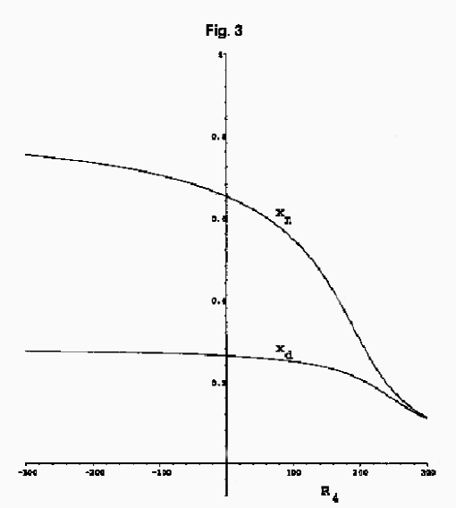
Figure 3: The $R_{4}$-dependence of the first positive numerator zero $(x_{n})$ and the first positive denominator zero $(x_{d})$ of the $[2|2]$ Padé-summation of the QCD $\beta$-function when $n_{f}=0$. The independent variable $R_{4}\equiv\beta_{4}/\beta_{0}$ is proportional to the presently unknown 5-loop contribution $(\beta_{4})$ to the $\beta$-function. The figure shows that $x_{d}$ and $x_{n}$ both exist over the entire range of $R_{4}$. However, $x_{d}$ always precedes $x_{n}$, indicative of the dynamics of Figure 2 for the evolution of the couplant $x(\mu)$ from the asymptotically-free ultraviolet region.

Figure 3 exhibits a plot of $x_{n}$, the first positive zero of (3.5), and $x_{d}$ (the first positive denominator zero of (3.5), as a function of the independent variable $R_{4}$. Such positive zeros are seen to occur for all $R_{4}$. Moreover, the first positive denominator zero is seen to precede the first positive numerator zero over the entire range of $R_{4}$. This last result confirms that the Fig. 2 dynamics predicted from $[1|2]$ and $[2|1]$ approximants appear to be stable against 5-loop corrections of arbitrary magnitude.

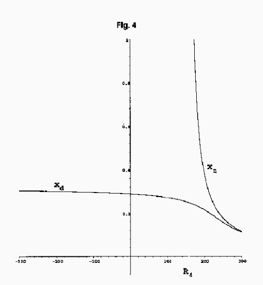
Figure 4: The $R_{4}$-dependence $[R_{4}\equiv\beta_{4}/\beta_{0}]$ of the first positive numerator zero $(x_{n})$ and the first positive denominator zero $(x_{d})$ of the $[1|3]$ Padé-summation of the QCD $\beta$-function when $n_{f}=0$. The figure shows that $x_{d}$ exists over the entire range of $R_{4}$. Moreover, $x_{d}$ precedes $x_{n}$ over the range of $R_{4}$ for which a positive numerator zero exists, leading once again to the dynamics of Figure 2 for the evolution of the couplant from the asymptotically-free ultraviolet region.

These results are corroborated by $\beta^{[1|3]}$ and $\beta^{[3|1]}$. Figure 4 plots the first positive numerator and denominator zeros of (3.6) against $R_{4}$ for $\beta^{[1|3]}$, as given by (3.6). A positive numerator zero $(x_{n})$ exists only if $R_{4}>150$, whereas at least one positive denominator zero $(x_{d})$ occurs for all $R_{4}$. Once again, however, $x_{d}$ precedes $x_{n}$ over the entire range of $R_{4}$, suggesting that $x_{d}$ exists as an infrared-attractor for all values of $R_{4}$. Moreover, the ordering $0<x_{d}<x_{n}$, over all values of $R_{4}$ for which $x_{n}$ exists, precludes any identification of $x_{n}$ with an infrared-stable fixed point.

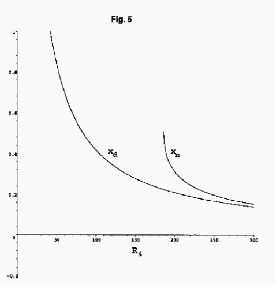
Figure 5: The $R_{4}$-dependence $[R_{4}\equiv\beta_{4}/\beta_{0}]$ of the first positive numerator zero $(x_{n})$ and the first positive denominator zero $(x_{d})$ of the $[3|1]$ Padé-summation of the QCD $\beta$-function when $n_{f}=0$. As in Figures 3 and 4, $x_{d}$ exists over the entire range of $R_{4}$, and $x_{d}$ precedes $x_{n}$ where a positive numerator zero exists.

Figure 5 plots $x_{n}$ and $x_{d}$ against $R_{4}$ for $\beta^{[3|1]}$, as given in (3.7). This case is perhaps the most interesting of all, as a positive denominator root $x_{d}$ is possible only if $R_{4}>0$, as is evident from the denominator of (3.7). Figure 5 shows that $x_{d}$ continues to precede $x_{n}$ for all positive values of $R_{4}$. Moreover, when $R_{4}$ is negative (and a positive pole $x_{d}$ is no longer possible), one sees from (3.7) that the numerator polynomial coefficients are all positive-definite, precluding any possibility of positive numerator roots. We thus see that an infrared-stable fixed point for $\beta^{[3|1]}$ is unattainable, even for the $R_{4}<0$ region for which no denominator zero occurs at all.

Thus, there does not exist any valid $N+M=4$ approximant $(M>0)$ to the $n_{f}=0$ QCD $\beta$-function which supports an infrared-stable fixed point, regardless of the magnitude of the presently unknown 5-loop term entering such approximants. Moreover, the Fig. 2 dynamics following from a positive $\beta$-function pole preceding any $\beta$-function zeros appear to be upheld not only by $[2|1]$- and $[1|2]$-approximant $\beta$-functions, but also by $[2|2]$-, $[1|3]$- and (when $R_{4}>0$) $[3|1]$-approximant $\beta$-functions as well.

One can also utilize asymptotic Padé approximant methods to estimate the magnitude of the infrared attractor (Fig. 2), corresponding to the first positive denominator zero of all the approximants considered so far. An asymptotic error formula [1] enables one to obtain an asymptotic Padé-approximant prediction (APAP) of $R_{4}$ from the three preceding terms $\{R_{1},R_{2},R_{3}\}$ in the $\beta$-function series [3]:

$$R_{4}^{APAP}=\frac{R_{3}^{2}}{R_{2}}\frac{[R_{2}^{3}+R_{1}R_{2}R_{3}-2R_{1}^{3}R_{3}]}{[2R_{2}^{3}-R_{1}^{3}R_{3}-R_{1}^{2}R_{2}^{2}]}.$$ (3.8)

Utilizing the values $\{R_{1},R_{2},R_{3}\}$ listed in Table 1 for $n_{f}=0$, one finds from (3.8) that $R_{4}^{APAP}=302.2$. If one inserts this value of $R_{4}$ into the $[2|2]$-, $[1|3]$- and $[3|1]$-approximant $\beta$-functions (3.5), (3.6) and (3.7), one finds reasonable agreement from all three $\beta$-functions as to the location of the first positive denominator zero, i.e. the infrared-attractor of Fig. 2. This zero is seen to occur at $x_{d}=0.11$ for $\beta^{[2|2]}$ and $\beta^{[1|3]}$, and at $x_{d}=0.14$ for $\beta^{[3|1]}$, corresponding to values of $\alpha_{s}$ between 0.35 and 0.44. A similar $R_{4}$-estimate ($R_{4}=270$) can be obtained for the $n_{f}=0$ case via the weighted asymptotic Padé approximant procedure (WAPAP) delineated in Section 5 of ref. [1]. This procedure expresses the coefficient $\beta_{4}=\beta_{0}R_{4}$ as a degree-4 polynomial in $n_{f}$, as would be obtained from an explicit perturbative calculation. We reiterate that the $n_{f}=0$ case minimizes unknown quadratic Casimir effects and avoids entirely the large uncertainties associated with the cancellation of large $n_{f}$-dependent terms within $\beta_{4}$ (as evident from eq. (5.5) of [1]) that characterize $n_{f}>0$ estimates based on APAP and WAPAP methods.

We conclude this section by reiterating that the ordering $0<x_{d}<x_{n}$ of positive denominator and numerator zeros of $n_{f}=0$ Padé-approximant $\beta$-functions suggests the existence of a double-valued couplant (Fig. 2), as already seen in SUSY gluodynamics [10]. Such a scenario is seen to decouple the infrared region $(\mu<\mu_{c})$ from the domain of purely-perturbative QCD, the domain of (real) $\alpha_{s}$. Such a scenario is perhaps also indicative of an additional phase distinguished by strong coupling dynamics at short distances Taking the Padé-approximants of the $\beta$-function seriously, one concludes that there is an ultraviolet-stable fixed point in that phase. Recall that in SUSY gluodynamics, such a fixed point is at $x=\infty$ [10]. Of course, it is impossible to assert that this ultraviolet-stable fixed point survives in the exact $\beta$-function of (non-SUSY) gluodynamics. For example, it may be replaced by an ultraviolet Landau pole.

Regardless of these considerations, the picture with an infrared attractor seems plausible and self-consistent. In such dynamics, both phases may share common infrared properties [10]. The presence of two phases has implications meriting further exploration. Such dynamics are shown in the Appendix to characterize QCD in the $N_{c}\rightarrow\infty$ limit for all but the aforementioned $[3|1]$-case with $R_{4}$ negative. Indeed, such dynamics may prove pertinent to the unexpected agreement between the glueball mass spectra obtained via lattice methods [23] and those obtained via supergravity wave equations in a black hole geometry [24] following from conjectured duality to large-N_c gauge theories [25], an agreement obtained despite the large bare coupling constant necessarily utilized in the latter approach.

In the section which follows, we extend the analysis of the QCD $\beta$-function to nonzero $n_{f}$ values. We specifically seek to address whether Padé-methods indicate a flavour-threshold for infrared-stable fixed points. However, we also seek insight as to whether there is any evidence for a strong phase of QCD when $n_{f}>0$, as such a phase could (conceivably) provide a dynamical mechanism for electroweak symmetry breaking.

4 QCD with Fermions

In this Section, we repeat the analysis of the previous section with $n_{f}\leq 16$ fermion flavours. The $n_{f}=16$ case is the maximum number of flavours consistent with asymptotic freedom: a $\beta$-function whose sign is negative as $x\rightarrow 0^{+}$.

4.1 Four-Loop-Level Results

We first consider the $\beta$-function (2.12) incorporating a $[2|1]$ approximant to describe post-one-loop behaviour. This $\beta$-function is fully determined by the known two-, three-, and four-loop terms $\{R_{1},R_{2},R_{3}\}$ tabulated in Table 1 for $n_{f}=\{1,2,...,16\}$. The values of the coefficients $\{a_{1},a_{2},b_{1}\}$ characterizing $\beta^{[2|1]}$ in (2.12a) are tabulated in Table 5. Also tabulated in the table are values for $x_{n}$, the first positive zero of the numerator $1+a_{1}x+a_{2}x^{2}$, as well as $x_{d}$, the zero of the denominator $1+b_{1}x$. Blank entries for $x_{n},x_{d}$ correspond to cases where no positive zero exists. We see from the table that a positive denominator zero precedes the first positive numerator zero for $n_{f}\leq 5$, in which case that denominator zero serves as an infrared attractor for both a strong and an asymptotically-free ultraviolet phase of the QCD couplant. The denominator zero becomes negative for $n_{f}\geq 6$; nevertheless, an infrared-stable fixed point (associated with a positive numerator zero) does not occur until $n_{f}=7$, as no positive numerator zero exists for $n_{f}=6$. The value of $x_{n}=\alpha_{s}/\pi$ associated with this infrared-stable fixed point decreases as $n_{f}$ increases, as anticipated in other work [13, 14]. If we regard $\alpha_{cr}=\pi/4$ ($x_{n}=1/4$) as the threshold value for chiral symmetry breaking [26], we see that the conformal window for QCD is predicted to begin at $n_{f}=11$. For $n_{f}=\{7-10\}$, the infrared-stable fixed point $x_{n}$ is not expected to govern infrared dynamics. Chiral-symmetry breaking should occur before the couplant reaches $x_{n}$, and the (now-massive) fermions are expected to decouple from further infrared evolution of $\alpha_{s}$ [13, 14].

$n_{f}$	$a_{1}$	$a_{2}$	$b_{1}$	$x_{n}$	$x_{d}$
0	-2.79959	-3.74745	-5.11777	0.26394	0.19540
1	-2.75323	-3.63638	-4.91452	0.26820	0.20350
2	-2.76977	-3.64714	-4.75253	0.26710	0.21041
3	-2.91691	-3.87504	-4.69468	0.25586	0.21301
4	-3.40349	-4.56534	-4.94349	0.22557	0.20229
5	-5.40850	-6.93442	-6.66937	0.15435	0.14994
6	19.9461	17.3690	19.01757	—	—
7	1.57664	-1.75513	1.05033	1.3275	—
8	0.245617	-4.66133	0.216205	0.49027	—
9	-0.337065	-7.66401	0.262935	0.33990	—
10	-0.839249	-11.8754	0.583828	0.25699	—
11	-1.49942	-18.3271	1.04603	0.19624	—
12	-2.56052	-28.7791	1.60615	0.14716	—
13	-4.46609	-46.9517	2.24819	0.10593	—
14	-8.33265	-82.5220	2.96735	0.070620	—
15	-18.2356	-171.036	3.76441	0.039903	—
16	-70.8563	-632.698	4.64367	0.012678	—

Table 5: The coefficients $a_{1}$, $a_{2}$ and $b_{1}$ in $\beta^{[2|1]}$, as given in Eq. (2.12) for $n_{f}=0-16$. The column $x_{n}$ tabulates the first positive zero of the numerator. The column $x_{d}$ tabulates the denominator zero, if positive. For those values of $n_{f}$ for which real positive numerator (denominator) zeros do not exist, the corresponding entries for $x_{n}\;(x_{d})$ are left blank. The table shows $0<x_{d}<x_{n}$ for $n_{f}\leq 5$, corresponding to Fig. 2 type dynamics for this range of $n_{f}$. When $n_{f}\geq 7$, $x_{n}$ corresponds to an infrared-stable fixed point that decreases as $n_{f}$ increases.

Qualitatively similar conclusions are obtained from the analysis of $\beta^{[1|2]}$ [eq. (2.13)], although the corresponding values of $n_{f}$-thresholds for various infrared properties differ somewhat from those of the $[2|1]$-approximant case. In Table 6 the values of the constants $\{a_{1},b_{1},b_{2}\}$ characterizing $\beta^{[1|2]}$ in (2.13a) are tabulated using the known values for $\{R_{1},R_{2},R_{3}\}$ listed in Table 1. When positive, the zero of the numerator $1+a_{1}x$ fails to precede positive zeros of the denominator $1+b_{1}x+b_{2}x^{2}$ until $n_{f}=9$ (positive denominator zeros cease occurring after $n_{f}=6$, but the numerator zero is negative when $5\leq n_{f}\leq 8$). Consequently, $n_{f}=9$ is the flavour-threshold for identification of $x_{n}$ as an infrared-stable fixed point. As before, this fixed point decreases with increasing $n_{f}$. Its magnitude does not fall below the $x_{n}=1/4$ threshold for chiral-symmetry breakdown until $n_{f}=12$, corresponding to a previous prediction [13] of the threshold for QCD’s conformal window, consistent with the qualitative picture presented in ref. [14]. Specific predictions for $x_{n}$ from Tables 5 and 6 agree quantitatively only within this $12\leq n_{f}\leq 16$ window. Although the intermediate range of $n_{f}$ for which $x_{n}>1/4$ differs between the two approximants ($7\leq n_{f}\leq 10$ for $\beta^{[2|1]}$; $9\leq n_{f}\leq 11$ for $\beta^{[1|2]}$), it is nevertheless significant that such a range exists for both cases. In Table 6, a positive denominator zero is seen to precede any positive numerator zeros when $n_{f}\leq 6$. This behaviour corresponds to the infrared dynamics suggested by Figure 2. Once again, qualitative agreement is seen to occur between the $[2|1]$- and $[1|2]$-approximant $\beta$-functions insofar as both $\beta$- functions predict dynamics governed by a $\beta$-function pole $x_{d}$ for $n_{f}$ less than some threshold value ($n_{f}\leq 5$ for $\beta^{[2|1]}$; $n_{f}\leq 6$ for $\beta^{[1|2]}$).

$n_{f}$	$a_{1}$	$b_{1}$	$b_{2}$	$x_{n}$	$x_{d}$
0	-5.96723	-8.28541	11.0906	0.16758	0.15136
1	-6.14941	-8.31070	10.9765	0.16262	0.15007
2	-6.68998	-8.67274	11.4200	0.14948	0.14177
3	-8.17337	-9.95114	13.2199	0.12235	0.11944
4	-13.8032	-15.3432	20.5809	0.072447	0.072160
5	70.6188	69.3580	-88.9261	—	0.79411
6	5.95098	5.02241	-4.37349	—	1.32141
7	1.93401	1.40769	1.56704	—	—
8	0.274983	0.245571	4.66047	—	—
9	-0.921639	-0.321639	7.31327	1.0850	—
10	-2.13228	-0.709208	10.0353	0.46898	—
11	-3.60614	-1.06069	12.9645	0.27730	—
12	-5.60030	-1.43363	16.1133	0.17856	—
13	-8.56349	-1.84921	19.4406	0.11677	—
14	-13.6105	-2.31052	22.8821	0.073472	—
15	-24.8114	-2.81137	26.3685	0.040304	—
16	-78.8413	-3.34126	29.8352	0.012684	—

Table 6: The coefficients $a_{1}$, $b_{1}$ and $b_{2}$ in $\beta^{[1|2]}$ as given in Eq. (2.13) for $n_{f}=0-16$. The column $x_{d}$ tabulates the first positive denominator zero. The column $x_{n}$ tabulates the numerator zero, if positive. For those values of $n_{f}$ for which real positive denominator (numerator) zeros do not exist, the corresponding entries for $x_{d}\;(x_{n})$ are left blank. The positive denominator zero $x_{d}$ occurs before any positive numerator zeros for $n_{f}\leq 6$, suggesting Fig. 2 type dynamics. When $n_{f}\geq 9$, $x_{n}$ corresponds to an infrared-stable fixed point that decreases as $n_{f}$ increases

4.2 Five-Loop Level Results

It is of interest to examine the stability of the qualitative results described above against five-loop corrections to the $\overline{MS}$ $\beta$-function, corrections which do not enter our determination of $\beta^{[2|1]}$ and $\beta^{[1|2]}$. As noted in Section 2, Padé-coefficients within $\beta^{[2|2]}$, $\beta^{[1|3]}$ and $\beta^{[3|1]}$ are all seen to be linear in the five-loop $\beta$-function correction $\beta_{4}$ ($\beta_{4}/\beta_{0}\equiv R_{4}$). These coefficients, as defined by equations (2.14a), (2.15a), and (2.16a), are respectively tabulated in Tables 2, 3 and 4. In Table 7 we have tabulated the domain of $R_{4}$ for which the first positive numerator zero of the Padé-approximant $\beta$-function precedes any positive denominator zero. Such a numerator zero implies a couplant with Figure 1 type dynamics, in which the numerator zero is an infrared-stable fixed point. We see from Table 7 that such dynamics do not occur at all regardless of $R_{4}$ unless $n_{f}\geq 6$. An infrared-stable fixed point cannot occur for $\beta^{[2|2]}$ until $n_{f}=7$ (and then only for $R_{4}<0$), nor can it occur for $\beta^{[1|3]}$ until $n_{f}=9$. As $n_{f}$ increases, the domain of $R_{4}$ for which Figure 1 type dynamics become possible is seen to broaden for all three Padé-approximant $\beta$-functions. The overall picture that emerges is quite similar to that anticipated from Tables 5 and 6. In every case, dynamics governed by an infrared-stable fixed point (Fig. 1) do not occur below a threshold value of $n_{f}$, a threshold at or above $n_{f}=6$.

Table 8 tabulates the range of $R_{4}$ for which a positive pole of $\beta^{[2|2]}$, $\beta^{[1|3]}$ and $\beta^{[3|1]}$ exists and precedes any positive numerator zeros, corresponding to the dynamics schematically presented in Figure 2. For $n_{f}\leq 5$, $\beta^{[2|2]}$ and $\beta^{[1|3]}$ are seen to exhibit such dynamics regardless of the magnitude of $R_{4}$, the five-loop contribution to the $\beta$-function. $\beta^{[3|1]}$ exhibits such Figure 2 type dynamics only if $R_{4}$ is positive, as the denominator $1+b_{1}x$ of eq. (2.16a) has a positive zero only if $R_{4}>0$ $[b_{1}=-R_{4}/R_{3}]$. Such dynamics, however, become impossible for $\beta^{[1|3]}$ and unlikely for $\beta^{[2|2]}$ and $\beta^{[3|1]}$ once $n_{f}$ gets sufficiently large, as is apparent in Table 8 from the steadily increasing lower bound on $R_{4}$ for such dynamics to occur within $\beta^{[2|2]}$ and $\beta^{[3|1]}$.

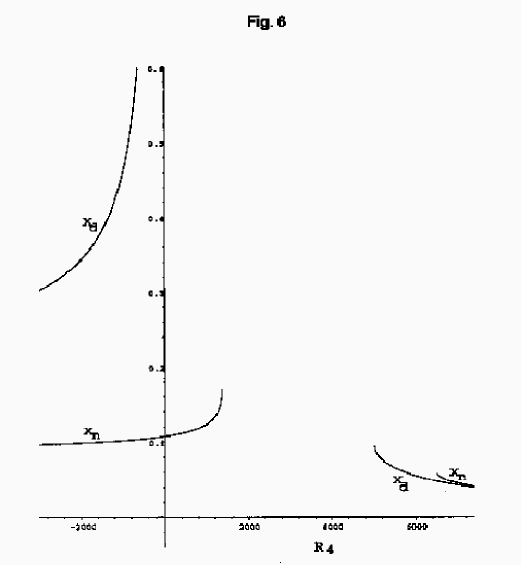
Figure 6: The behaviour over a very large region of $R_{4}$ of the first positive numerator zero $(x_{n}$) and the first positive denominator zero $(x_{d})$ of the $[2|2]$ Padé-summation of the QCD $\beta$-function when $n_{f}=13$. The figure shows that $x_{n}$ precedes $x_{d}$ when $R_{4}<1383$, indicative of dynamics governed by an infrared-stable fixed point (Figure 1) for this region. The figure also shows that $x_{d}$ precedes $x_{n}$ when $R_{4}$ is very large ($R_{4}>5020$), indicative of dynamics governed by a $\beta$-function pole (Figure 2). The absence of a positive $\beta$-function zero for $R_{4}$ between 1383 and 5020 precludes the possibility of dynamics governed by an infrared-stable fixed point for this range of $R_{4}$.

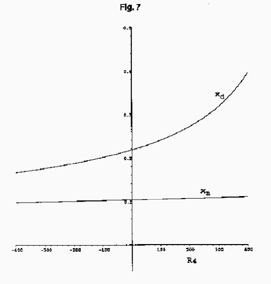
Figure 7: The $R_{4}$-dependence of the first positive numerator zero $(x_{n})$ and the first positive denominator zero $(x_{d})$ of the $[1|3]$ Padé-summation of the QCD $\beta$-function when $n_{f}=13$. The numerator zero is seen to precede the denominator zero over the entire range of $R_{4}$ exhibited, consistent with the numerator zero serving as an infrared-stable fixed point. This numerator zero ceases to be positive when $R_{4}>6394$.

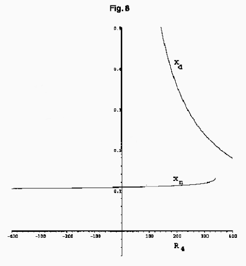
Figure 8: The $R_{4}$-dependence of the first positive numerator zero $(x_{n})$ and the first positive denominator zero $(x_{d})$ of the $[3|1]$ Padé-summation of the QCD $\beta$-function when $n_{f}=13$. The numerator zero is seen to precede the denominator zero when $R_{4}<340$, corresponding to the domain of $R_{4}$ for dynamics governed by the infrared-stable fixed point $x_{n}$. The denominator zero precedes any positive numerator zeros that occur for $R_{4}>340$, corresponding to Figure 2 dynamics governed by an infrared attractor at $x_{d}$.

This large $n_{f}$ behaviour is illustrated for $n_{f}=13$ by plots of the $R_{4}$-dependence of the first positive numerator and denominator zero of $\beta^{[2|2]}$ (Fig. 6), $\beta^{[1|3]}$ (Fig. 7) and $\beta^{[3|1]}$ (Fig. 8). The infrared-stable fixed point associated with the numerator zero in $\beta^{[2|2]}$ and $\beta^{[3|1]}$ is seen to be less than 1/4 (the assumed threshold for chiral-symmetry breakdown [26]) over the full domain of $R_{4}$ indicated in Table 7 for infrared-stable fixed point dynamics, a result is clearly suggestive of $n_{f}=13$ being within the conformal window of QCD. The numerator zero in $\beta^{[1|3]}$ is also below 1/4, as evident from Fig. 7, until the immediate neighbourhood of its singularity at $R_{4}=6394$.

$n_{f}$	$[2|2]$	$[1|3]$	$[3|1]$
0	No $R_{4}$	No$R_{4}$	No$R_{4}$
1	No $R_{4}$	No$R_{4}$	No$R_{4}$
2	No $R_{4}$	No$R_{4}$	No$R_{4}$
3	No $R_{4}$	No$R_{4}$	No$R_{4}$
4	No $R_{4}$	No$R_{4}$	No$R_{4}$
5	No $R_{4}$	No$R_{4}$	No$R_{4}$
6	No $R_{4}$	No$R_{4}$	$R_{4}<-105$
7	$R_{4}<0.21$	No$R_{4}$	$R_{4}<-2.1$
8	$R_{4}<21.6$	No$R_{4}$	$R_{4}<1.2$
9	$R_{4}<57.2$	$R_{4}<62.3$	$R_{4}<3.6$
10	$R_{4}<128.4$	$R_{4}<174.9$	$R_{4}<12.9$
11	$R_{4}<274.6$	$R_{4}<508.5$	$R_{4}<38.4$
12	$R_{4}<594.9$	$R_{4}<1644$	$R_{4}<110$
13	$R_{4}<1384$	$R_{4}<6394$	$R_{4}<340.3$
14	$R_{4}<3750$	$R_{4}<34187$	$R_{4}<1226$
15	$R_{4}<14262$	$R_{4}<355521$	$R_{4}<6057$
16	$R_{4}<174589$	$R_{4}<37198800$	$R_{4}<92883$

Table 7: The domain of $R_{4}$ for which an infrared fixed point occurs for $\beta^{[2|2]}$, $\beta^{[1|3]}$ and $\beta^{[3|1]}$. The ranges of $R_{4}$ listed (for a given choice of $n_{f}$) are those for which a positive numerator zero exists and precedes any positive denominator zeros of the Padé-approximant $\beta$-function.

$n_{f}$	$[2|2]$	$[1|3]$	$[3|1]$
0	All $R_{4}$	All $R_{4}$	$R_{4}>0$
1	All $R_{4}$	All $R_{4}$	$R_{4}>0$
2	All $R_{4}$	All $R_{4}$	$R_{4}>0$
3	All $R_{4}$	All $R_{4}$	$R_{4}>0$
4	All $R_{4}$	All $R_{4}$	$R_{4}>0$
5	All $R_{4}$	All $R_{4}$	$R_{4}>0$
6	$R_{4}>-105$	$R_{4}>-35.4$	$R_{4}>0$
7	No $R_{4}$	$R_{4}>0.2$	$R_{4}>0$
8	No $R_{4}$	$R_{4}>21.5$	$R_{4}>1.2$
9	$R_{4}>4848$	No $R_{4}$	$R_{4}>3.6$
10	$R_{4}>2964$	No $R_{4}$	$R_{4}>12.9$
11	$R_{4}>2990$	No $R_{4}$	$R_{4}>38.4$
12	$R_{4}>3652$	No $R_{4}$	$R_{4}>110$
13	$R_{4}>5020$	No $R_{4}$	$R_{4}>340.3$
14	$R_{4}>7759$	No $R_{4}$	$R_{4}>1226$
15	$R_{4}>14491$	No $R_{4}$	$R_{4}>6057$
16	$R_{4}>174589$	No $R_{4}$	$R_{4}>92883$

Table 8: The domain of $R_{4}$ for which a positive denominator zero exists and precedes any positive numerator zeros of $\beta^{[2|2]}$, $\beta^{[1|3]}$ and $\beta^{[3|1]}$, respectively. Such a condition corresponds to the Figure 2 scenario for coupling constant evolution, in which the positive denominator zero is an infrared attractor for both a strong and weak phase of the couplant.

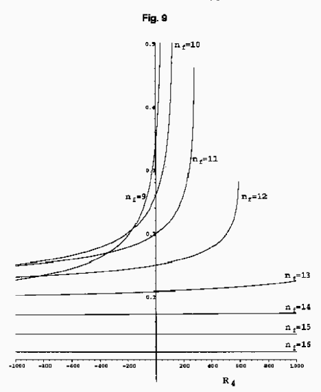
Figure 9: The $n_{f}$-dependence of the infrared fixed point $x_{n}$, as indicated by successive plots of $x_{n}$ versus $R_{4}$ for $\beta^{[2|2]}$ with values of $n_{f}$ ranging from 9-16.

The decrease of the infrared fixed point with increasing $n_{f}$ is also common to all Padé-approximant $\beta$-functions. This behaviour, as already seen in Tables 5 and 6 for $\beta^{[2|1]}$ and $\beta^{[1|2]}$, is illustrated for $\beta^{[2|2]}$ in Fig. 9, in which the magnitudes of $x_{n}$ are displayed as functions of $R_{4}$ for $n_{f}=\{9-16\}$. Such results are consistent with the phase structure anticipated in ref. [14], as already noted. It is also worth mentioning that the general picture we obtain, particularly the need for a critical number of flavours for an infrared-stable fixed point to occur at all, agrees surprisingly well with a lattice study [27].

5 QCD’s Infrared Boundary

The case of three flavours is of obvious interest, as Padé-extrapolations to the infrared region can be compared to the known empirical dynamics at the onset of the infrared region. We know, for example, that evolution of the running coupling constant from its well-determined value at $\mu=M_{z}$ [28] leads to a prediction [3]

$$\alpha_{s}(n_{f}=3;\;\;\mu=1\;GeV)=0.48\begin{array}[]{c}+0.09\\ -0.07\end{array}$$ (5.1)

We also know that QCD as a theory of quarks and gluons ceases to exist at momentum scales approaching $\Lambda_{QCD}$, although the interpretation of $\Lambda_{QCD}$ is subject to redefinition for each successive order of perturbation theory.

Tables 5-7 show quite clearly that an infrared-stable fixed point for $n_{f}=3$ QCD is unsupported by all Padé-approximant $\beta$-functions considered here, regardless of the magnitude of $R_{4}$. This result contradicts the infrared-stable fixed point obtained from the analysis of a lower-order expression for the $\beta$-function in refs. [11] and [12], although the absence of such a fixed point at $n_{f}=3$ is supported by more recent work [17]. We also note that all Padé- approximant $\beta$-functions considered here exhibit Figure 2 type dynamics, regardless of $R_{4}$, except for $\beta^{[3|1]}$ when $R_{4}<0$. In such dynamics, the $\beta$-function pole $x_{d}$ occurs at momentum-scale $\mu_{c}$. As evident from Fig. 2, the infrared region $\mu<\mu_{c}$ is inaccessible to the (real) couplant $x(\mu)$, suggesting that $\mu_{c}$ fulfills the infrared cutoff role commonly ascribed to $\Lambda_{QCD}$, the “Landau pole” obtained through use of the truncated $\beta$-function series.

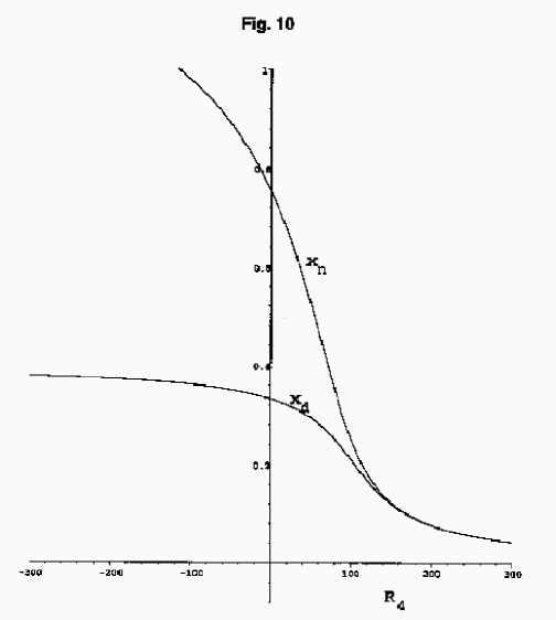
Figure 10: The $R_{4}$-dependence of the first positive numerator zero $(x_{n})$ and the first positive denominator zero $(x_{d})$ of the $[2|2]$ Padé-summation of the QCD $\beta$-function when $n_{f}=3$. The figure shows that $x_{d}$ always precedes $x_{n}$, indicative of infrared-attractor dynamics (Figure 2).

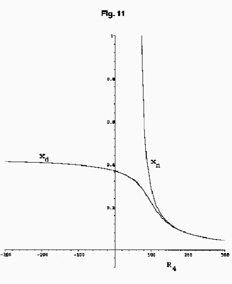
Figure 11: The $R_{4}$-dependence of the first positive numerator zero $(x_{n})$ and the first positive denominator zero $(x_{d})$ of the $[1|3]$ Padé-summation of the QCD $\beta$-function when $n_{f}=3$. The figure shows that $x_{d}$ exists over the entire range of $R_{4}$, and precedes $x_{n}$ over the range where such a positive zero exists. Hence $x_{d}$ serves as an infrared attractor.

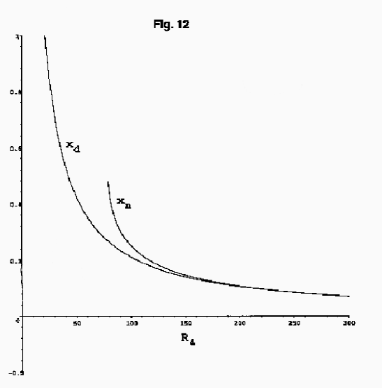
Figure 12: The $R_{4}$-dependence of the first positive numerator zero $(x_{n})$ and the first positive denominator zero $(x_{d})$ of the $[3|1]$ Padé-summation of the QCD $\beta$-function when $n_{f}=3$. The figure shows that $x_{d}$ exists over the entire range of $R_{4}$, and precedes $x_{n}$ over the range where such a positive zero exists, as in Fig. 11. Hence $x_{d}$ serves as an infrared attractor for this case as well.

In Figs. 10-12, we have exhibited the $R_{4}$ dependence of the $\beta$- function pole $x_{d}$ for $\beta^{[2|2]}$, $\beta^{[1|3]}$ and $\beta^{[3|1]}$ when $n_{f}=3$. The first positive numerator zero is also displayed in all three figures, and is seen to be larger than $x_{d}$ for all $R_{4}$ values considered. We note from Figs. 10 and 11 the apparent stability of $x_{d}$ in $\beta^{[2|2]}$ and $\beta^{[1|3]}$ against changes in $R_{4}$ when $R_{4}$ is negative. Both figures indicate an infrared-attractor near $x_{d}=0.4$ $(\alpha_{s}\cong 1.3)$, a value well-above the anticipated threshold for chiral-symmetry breaking.

Given knowledge of an initial value, one can utilize Padé approximant $\beta$-functions to estimate the infrared cutoff $\mu_{c}$. To demonstrate this, we assume from the central value of (5.1) that $x(1\;GeV)=\alpha_{s}(1\;GeV)/\pi=0.153$. The equation

$$\mu^{2}\frac{dx}{d\mu^{2}}=\beta^{[N|M]}(x)$$ (5.2)

can be inverted to determine $\mu_{c}$ the value of $\mu$ corresponding to the first positive pole of $\beta^{[N|M]}$, Figure 2’s infrared attractor $x_{d}=x(\mu_{c})$:

$$\mu_{c}(GeV)=exp\left[\frac{1}{2}\int_{x(1GeV)}^{x_{d}}\frac{dx^{\prime}}{\beta^{[N|M]}(x^{\prime})}\right]$$ (5.3)

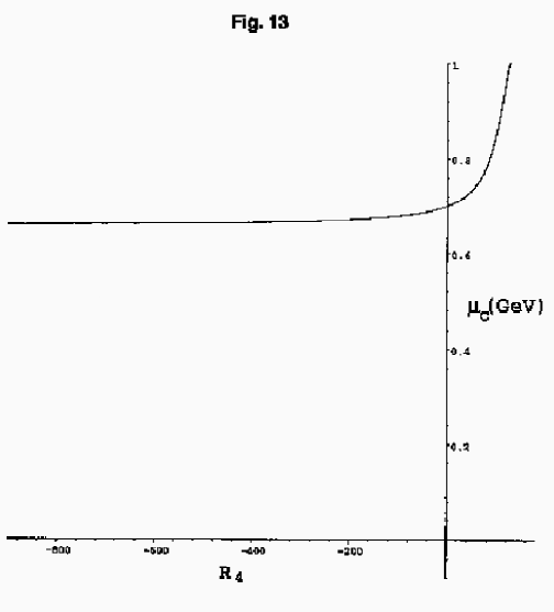
Figure 13: The $R_{4}$-dependence of $\mu_{c}$, the minimum value of $\mu$ accessible to the couplant $x(\mu)$ derived from $\beta^{[2|2]}$ when $n_{f}=3$. The 1 GeV value of the couplant is assumed to be x(1) = 0.153, as discussed in the text

We have utilized (5.3) to plot predicted values of $\mu_{c}$ for $[2|2]$; $[1|3]$; and $[3|1]$-approximant $\beta$-functions against the unknown 5-loop $\beta$-function coefficient $R_{4}(\equiv\beta_{4}/\beta_{0})$. Fig. 13 utilizes $\beta^{[2|2]}$, as determined by the $n_{f}=3$ row of Table 2, to predict $\mu_{c}$, given $x(1)=0.153$. The curve terminates with $\mu_{c}=1\;GeV$ at $R_{4}=128$, since $x_{d}$ (the infrared attractor) is itself equal to 0.153 at this value of $R_{4}$. What is noteworthy, however, is the stability of $\mu_{c}$ over the entire range of negative $R_{4}$. Fig. 13 is clearly indicative of QCD’s infrared cutoff (mass gap) occurring not much below the $\rho$ mass: $\mu_{c}\rightarrow 660\;MeV$ as $R_{4}\rightarrow-\infty$.

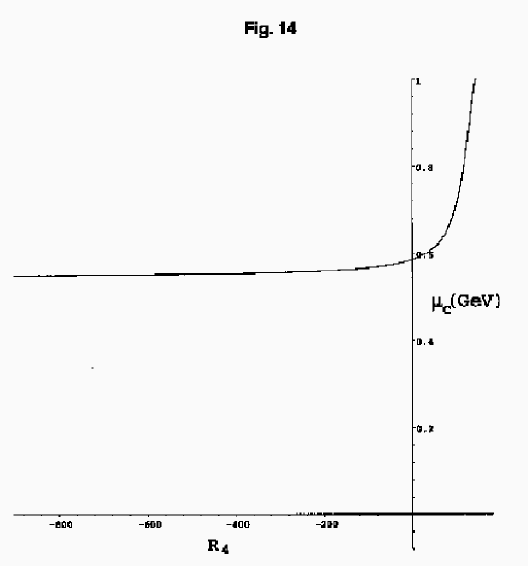
Figure 14: The $R_{4}$-dependence of $\mu_{c}$, as in Figure 13, except that the 1 GeV value of the couplant is given a lower-bound value $x(1)$ = 0.1305.

Thus Fig. 13 is indicative of a lower bound for $\mu_{c}$ well-above the phenomenological value for $\Lambda_{QCD}$ when $n_{f}=3$. The bound on $\mu_{c}$ obtained from $\beta^{[2|2]}$ remains well above $\Lambda_{QCD}$ even if the estimate for $\alpha_{s}(1\;GeV)$ is reduced to the floor of its empirical range. Fig. 14 utilizes $\beta^{[2|2]}$ in conjunction with the lower-bound value of (5.1) for $\alpha_{s}(1\;GeV)$ $\left[x(1)=\alpha_{s}(1\;GeV)/\pi=0.1305\right]$. The figure continues to predict insensitivity to $R_{4}$ over the entire negative range of $R_{4}$, with a somewhat diminished lower bound on $\mu_{c}$: $\mu_{c}\rightarrow 550\;MeV$ from above as $R_{4}\rightarrow-\infty$.

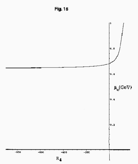
Figure 15: The $R_{4}$-dependence of $\mu_{c}$, the minimum value of $\mu$ accessible to the couplant $x(\mu)$ derived from $\beta^{[1|3]}$ when $n_{f}=3$ and $x(1)$ = 0.153.

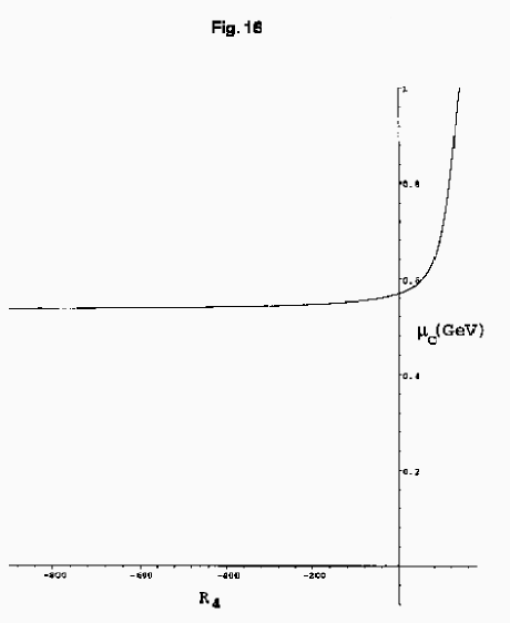
Figure 16: The $R_{4}$-dependence of $\mu_{c}$, as in Figure 15, except that the 1 GeV value of the couplant is given a lower-bound value $x(1)$ = 0.1305.

The behaviour described above is virtually identical to that obtained by utilizing $\beta^{[1|3]}$ within (5.3). Figures 13 and 14 display $\mu_{c}$ as a function of $R_{4}$, with $x(1)=0.153$ [Fig 15] and $x(1)=0.1305$ [Fig 16]. The expression for $\beta^{[1|3]}$ utilized in the integrand of (5.3) can be extracted from the $n_{f}=3$ row of Table 3. Both curves terminate at $\mu_{c}=1\;GeV$ at $R_{4}$ values corresponding to the infrared attractor $x_{d}$ being equal to $x(1\;GeV)$ [$x_{d}=0.153$ and $x_{d}=0.1305$, respectively]. Both curves also demonstrate the same stability of $\mu_{c}$ against changes in $R_{4}$, as well as virtually the same lower bounds for $\mu_{c}$ as obtained in Figs. 13 and 14 from $\beta^{[2|2]}$.

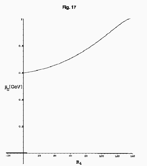
Figure 17: The $R_{4}$-dependence of $\mu_{c}$, the minimum value of $\mu$ accessible to the couplant $x(\mu)$ derived from $\beta^{[3|1]}$ when $n_{f}=3$ and $x(1)$ = 0.153. The couplant has an infrared attractor for this case only if $R_{4}$ is positive.

As noted earlier, an infrared attractor associated with an $n_{f}=3$ $\beta$-function pole occurs within $\beta^{[3|1]}$ only for $R_{4}>0$. In Fig. 17, we plot the $\beta^{[3|1]}$-prediction for the value of $\mu_{c}$, as obtained from (5.3), against positive values of $R_{4}$. Using the central value $x(1)=0.153$ from (4.1), we see that $\mu_{c}>600MeV$ over the entire (positive) range of $R_{4}$.

For $R_{4}<0$, $\beta^{[3|1]}(x)$ no longer has a pole. This does not mean, however, that $\alpha_{s}(\mu)$ has a domain in which $\mu$ can get arbitrarily close to zero. Rather, when $R_{4}<0$, there will exist a Landau pole, i.e. a minimum value of $\mu$ at which $\alpha_{s}$ will diverge:

$$\mu_{L}=exp\left(\frac{1}{2}\int_{x(1GeV)}^{\infty}\frac{dx}{\beta^{[3|1]}}\right)$$ (5.4)

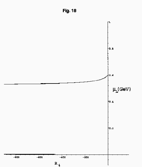
Figure 18: The $R_{4}$-dependence of the Landau pole $\mu_{L}$ of the couplant derived from $\beta^{[3|1]}$ when $n_{f}=3$ and $x(1)$ = 0.153. This Landau pole (as opposed to an infrared attractor of two ultraviolet phases) occurs only for negative values of $R_{4}$.

Similar dynamics characterize the evolution of $\alpha_{s}(\mu)$ that follows from the one-loop $\beta$-function [$\beta(x)=-\beta_{0}x^{2}$], even though this $\beta$-function itself has neither poles nor non-zero fixed points. We have utilized (5.4) in Fig. 18 to find the minimum value of $\mu$ as a function of $R_{4}$. If $x(1\;GeV)=0.153$, consistent with (5.1), we then find that $\mu_{L}$ approaches 530 MeV from above as $R_{4}\rightarrow-\infty$.

In every case we consider, it is clear that the domain of $\alpha_{s}(\mu)$ when $n_{f}=3$ is bounded from below by hadronic mass scales comparable to or somewhat below the $\rho$-mass. Padé-approximant $\beta$- functions appear to decouple the infrared region from $\alpha_{s}$ at values of $\mu$ substantially larger than $\Lambda_{QCD}$.

6 Conclusions

Utilizing Padé-summation QCD $\beta$-functions whose Maclaurin expansions reproduce the known terms of the $\overline{MS}$ $\beta$-function series, we obtain a surprising degree of agreement with infrared properties predicted [13, 14, 17] via the ’t Hooft renormalization scheme [29] in which the $\beta$-function is truncated subsequent to two-loop order. Within the context of $N_{c}=3$ QCD, we find clear evidence for a flavour-threshold between $n_{f}=6$ and $n_{f}=9$ for any possibility at all of infrared dynamics governed by an infrared-stable fixed point. For $n_{f}<6$, no approximant-based -function (other than the truncated series itself) is able to yield a positive zero that is not preceded by a positive pole, regardless of the as-yet-unknown magnitude of the five-loop contribution ($R_{4}$) to the $\overline{MS}$ $\beta$-function series (2.10). We reiterate that such a zero can be identified as an infrared-stable fixed point only if it is not preceded by a positive $\beta$-function pole.

We also find (Section 4) that when $n_{f}$ exceeds the (approximant-dependent) flavour threshold for possible infrared-stable fixed-point dynamics, the magnitude of that fixed point is seen to decrease as $n_{f}$ increases (Tables 5 and 6 and Figure 9). The true conformal window of QCD is not expected to begin until the infrared-stable fixed point is sufficiently small to preclude chiral-symmetry breaking in the infrared region [13, 14]. In Section 4, we corroborate this window’s onset at 11-13 flavours, as anticipated from two-loop results [13, 14].

For values of $n_{f}$ below the (approximant-dependent) threshold for a possible infrared-stable fixed point, Padé-summations of the $\overline{MS}$ $\beta$-function are indicative of infrared dynamics governed by a $\beta$-function pole, as has already been observed for N=1 SQCD in the absence of fundamental-representation matter fields [10]. Such a positive pole preceding all positive zeros of the $\beta$-function is found to occur for $n_{f}\leq 5$ for all Padé-approximant $\beta$-functions constructed from the $\overline{MS}$ $\beta$-function series, regardless of the unknown five-loop term ($R_{4}$) in that series, except for the $\beta$-function incorporating both a $[3|1]$-approximant to higher-loop effects and a negative value of $R_{4}$. Infrared dynamics governed by such a pole have a number of phenomenologically interesting properties. Salient among these is the occurrence of an infrared cut-off $\mu_{c}$ on the domain of the QCD couplant $\alpha_{s}(\mu)/\pi$ (Figure 2). We find (Figs. 13-17) the magnitude of $\mu_{c}$ to be quite stable against changes in $R_{4}$, and to be bounded from below by values larger than $\Lambda_{QCD}$ and comparable to low-lying meson masses (500-700 MeV). Such an infrared boundary occurs even for the $[3|1]$-approximant case with $R_{4}<0$, a case for which a positive $\beta$-function pole does not exist. For this case the infrared boundary corresponds to a Landau pole at similar hadronic mass scales (Fig. 18).

Pole-dominated infrared dynamics have also been argued [10] to imply the existence of a strong phase that devolves to the same infrared attractor as the asymptotically-free phase of the QCD couplant. In such dynamics, both phases may share common infrared properties [10]. As we have noted at the end of Section 3, such dynamics may provide a clue as to why lattice results for the glueball spectrum appear to be in agreement with results obtained in the strong-coupling, large-$N_{c}$ limit of $SU(N_{c})$ via supergravity wave equations within a black hole geometry.

Appendix: Gluodynamics in the ’t Hooft Limit

If the product of $N_{c}$ and $\alpha_{s}$ is finite and nonzero in the $N_{c}\rightarrow\infty$ limit, the $n_{f}=0\;{\overline{MS}}\;SU(N_{c})$ $\beta$- function in this same limit is given by [19]

$$\mu^{2}\frac{d\lambda}{d\mu^{2}}=-\frac{11}{3}\lambda^{2}\left[1+R_{1}\lambda+R_{2}\lambda^{2}+R_{3}\lambda^{3}(+\;R_{4}\lambda^{4}...)\right]$$ (A.1a)

$$\lambda\equiv N_{c}\alpha_{s}(\mu)/4\pi,$$ (A.1b)

$$R_{1}=34/11,$$ (A.1c)

$$R_{2}=2857/198,$$ (A.1d)

$$R_{3}=86.04326.$$ (A.1e)

The coefficients subsequent to $R_{3}$ in (A.1a) remain unknown at present. However, the known coefficients in (A.1a) are sufficient to determine Padé-summation functions incorporating $[2|1]$ and $[1|2]$ approximants via (2.12) and (2.13):

$$\beta^{[2|1]}(\lambda)=-\frac{11}{3}\lambda^{2}\frac{[1-2.87219\lambda-4.00209\lambda^{2}]}{[1-5.96310\lambda]}$$ (A.2)

$$\beta^{[1|2]}(\lambda)=-\frac{11}{3}\lambda^{2}\frac{[1-5.40935\lambda]}{[1-8.50026\lambda+11.8442\lambda^{2}]}.$$ (A.3)

In both of these approximations, the first positive zero of the denominator [0.1677 in (A.2) and 0.1483 in (A.3)] precedes the first positive zero of the numerator [0.2595 in (A.2) and 0.1849 in (A.3)], excluding Figure 1 type infrared-stable fixed point dynamics. Rather, both approximations support Figure 2 type dynamics, in which the first positive denominator zero ($\lambda_{d}$) serves as an infrared attractor for both a weak and a strong ultraviolet phase.

Such behaviour suggests that both phases may share common infrared properties, as the running couplants in both phases evolve towards the same infrared attractor. This behaviour is corroborated by $[1|3]$ and $[2|2]$ Padé-summation $\beta$-functions whose Maclaurin expansions reproduce (A.1a) inclusive of an arbitrary five-loop contribution $R_{4}$. For example, we find from comparison of (2.15) to (A.1a) that

$$\beta^{[1|3]}(\lambda)=-\frac{11}{3}\lambda^{2}\left[\frac{1+a_{1}\lambda}{1+b_{1}\lambda+b_{2}\lambda^{2}+b_{3}\lambda^{3}}\right];$$ (A.4a)

$$a_{1}=15.8424-0.0379166R_{4},$$ (A.4b)

$$b_{1}=12.7515-0.0379166R_{4},$$ (A.4c)

$$b_{2}=-53.8429+0.117197R_{4},$$ (A.4d)

$$b_{3}=-103.614+0.184865R_{4}.$$ (A.4e)

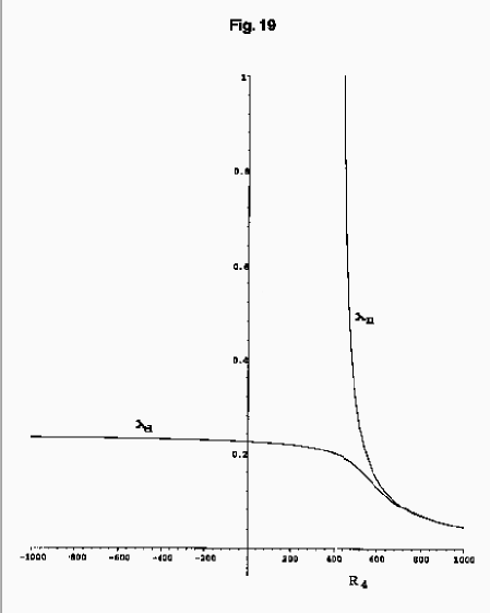
Figure 19: The dependence on the unknown five-loop term $R_{4}$ of the first positive numerator zero ($\lambda_{n}$) and the first positive denominator zero ($\lambda_{d}$) of the $[1|3]$ Padé-summation of the $SU(N_{c})$ $\beta$-function for the couplant $\lambda=N_{c}\alpha(\mu)/4\pi$ in the $N_{c}\rightarrow\infty$ limit ($n_{f}=0$). The figure shows that the denominator zero $\lambda_{d}$ exists over the range of $R_{4}$ and precedes the first positive numerator zero $\lambda_{n}$ when such a zero exists, indicative of Figure 2 dynamics with $\lambda_{d}$ serving as the infrared attractor.

In Figure 19 we have plotted the first positive numerator and denominator zeros of (A.4a) as a function of $R_{4}$, the unknown five-loop term. A positive denominator zero $(\lambda_{d})$ occurs over the entire range of $R_{4}$ and precedes the numerator zero $(\lambda_{n})$ when positive, consistent with Figure 2-type dynamics. For the $[2|2]$ case, we find from (2.16) and (A.1) that

$$\beta^{[2|2]}(\lambda)=-\frac{11}{3}\lambda^{2}\left[\frac{1+a_{1}\lambda+a_{2}\lambda^{2}}{1+b_{1}\lambda+b_{2}\lambda^{2}}\right];$$ (A.5a)

$$a_{1}=24.5902-0.0535237R_{4}$$ (A.5b)

$$a_{2}=-47.3211+0.0844278R_{4},$$ (A.5c)

$$b_{1}=21.4993-0.0535237R_{4},$$ (A.5d)

$$b_{2}=-128.203+0.249865R_{4}.$$ (A.5e)

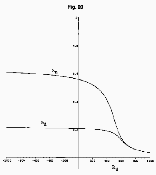
Figure 20: The $R_{4}$-dependence of the first positive numerator zero ($\lambda_{n}$) and the first positive denominator zero ($\lambda_{d}$) of the $[2|2]$ Padé-summation of the $SU(N_{c})$ $\beta$-function for the couplant $\lambda=N_{c}\alpha(\mu)/4\pi$ in the $N_{c}\rightarrow\infty$ limit ($n_{f}=0$). Once again, the denominator zero $\lambda_{d}$ exists over the entire range of $R_{4}$ and precedes the first positive numerator zero $\lambda_{n}$.

As is evident from Fig. 20, the first positive numerator zero $(\lambda_{n})$ is always preceded by a positive denominator zero $(\lambda_{d})$, which serves as the infrared-attractor for Figure 2-type dynamics, regardless of the unknown five-loop term $R_{4}$.

Incorporation of a $[3|1]$ approximant within the Padé-summation of (A.1) yields a positive denominator zero only if $R_{4}>0$. This is because $\lambda_{d}=R_{3}/R_{4}$, as is evident from (2.16a) and (2.16e). Hence, if $R_{4}<0$, infrared dynamics along the lines of Fig. 2 are no longer possible. However, we have found that no positive numerator zero exists for this regime, also excluding the possibility of Fig. 1 type dynamics governed by an infrared-stable fixed point. If $R_{4}$ is positive, the denominator zero is once again seen to precede all positive numerator zeros, again consistent with Figure 2 type dynamics. All of this behaviour can be extracted from (2.16) and (A.1):

$$\beta^{[3|1]}(\lambda)=-\frac{11}{3}\lambda^{2}\frac{[1+a_{1}\lambda+a_{2}\lambda^{2}+a_{3}\lambda^{3}]}{[1+b_{1}\lambda]}$$ (A.6a)

$$a_{1}=3.09091-0.0116221R_{4}$$ (A.6b)

$$a_{2}=14.2929-0.0359227R_{4},$$ (A.6c)

$$a_{3}=86.0433-0.167698R_{4},$$ (A.6d)

$$b_{1}=-0.0116221R_{4}.$$ (A.6e)

The absence of a positive numerator zero when $R_{4}$ is negative necessarily follows from the fact that $a_{1},a_{2}$, and $a_{3}$ are all positive when $R_{4}<0$.

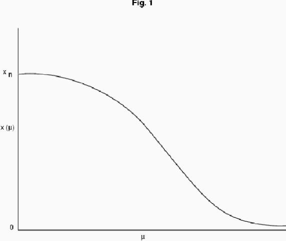
Figure 1: Behaviour of the asymptotically-free running couplant $x(\mu)\equiv\alpha_{s}(\mu)/\pi$ in dynamics governed by an infrared-stable fixed point $x_{n}$.

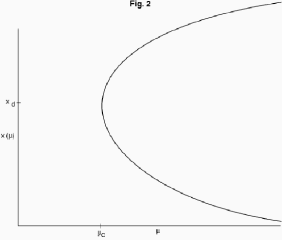
Figure 2: Behaviour of the asymptotically-free running couplant $x(\mu)$ in dynamics governed by a $\beta$-function pole at $x_{d}$. The point $x_{d}$ serves as an infrared attractor of both a strong and weak phase of the couplant. An infrared cut-off $\mu_{c}$ necessarily occurs, corresponding to the $\beta$-function pole at $x(\mu_{c})=x_{d}$.

References

- [1] J. Ellis, I. Jack, D.R.T. Jones, M. Karliner, and M. A. Samuel, Phys. Rev. D57 (1998), 2665.
- [2] J. Ellis, M. Karliner and M. A. Samuel, Phys. Lett. B400 (1997), 176.
- [3] V. Elias, T.G. Steele, F.Chishtie, R. Migneron and K. Sprague, Phys. Rev. D58 (1998), 116007.
- [4] F. Chishtie, V. Elias, T.G. Steele, Phys. Lett. B466 (1999), 267.
- [5] H. Kleinert, J. Neu, V. Schulte-Frohlinde, K.G. Chetyrkin and S. A. Larin, Phys. Lett. B272, 39 (1991); 319 (1993), 545 (E).
- [6] F. Chishtie, V. Elias, T.G. Steele, Phys. Rev. D59 (1999), 105013.
- [7] A.I. Vainshtein and V.I. Zakharov, Phys. Rev. Lett. 73 (1994), 1207.
-
[8]
M.A. Samuel, J. Ellis and M. Karliner, Phys. Rev. Lett.
74, 4380 (1995), 4380.
J. Ellis, E. Gardi, M. Karliner and M. A. Samuel, Phys. Lett. B366 (1996), 268 . - [9] E. Gardi, Phys. Rev. D56 (1997), 68.
- [10] I.I. Kogan and M. Shifman, Phys. Rev. Lett. 75 (1995), 2085.
-
[11]
A.C. Mattingly and P.M. Stevenson, Phys. Rev. Lett. 69(1992), 1320.
P.M. Stevenson, Phys. Lett. B331 (1994), 187. - [12] A.C. Mattingly and P. M. Stevenson. Phys. Rev. D49 (1994), 437.
-
[13]
T. Appelquist, J. Terning and L.C.R. Wijewardhana, Phys.
Rev. Lett. 77 (1996), 1214.
T. Appelquist, A. Ratnaweera, J. Terning and L.C.R. Wijewardhana, Phys. Rev. D58(1998), 105017.
T. Appelquist and F. Sannino, Phys. Rev. D59 (1999), 067702. -
[14]
V. A. Miransky and K. Yamawaki, Phys. Rev. D55
(1997), 5051 and Erratum 56 (1997), 3768.
V. A. Miransky, Phys. Rev. D59 (1999), 105003. - [15] R. S. Chivukula, Phys. Rev. D55 (1997), 5238.
- [16] M. Velkovsky and E. Shuryak, Phys. Lett. B437 (1998), 398.
-
[17]
E. Gardi and M. Karliner, Nucl. Phys. B529 (1998), 383.
E. Gardi, G. Grunberg and M. Karliner, JHEP 07 (1998), 007.
E. Gardi and G. Grunberg, JHEP 9903 (1999), 024. - [18] T. Banks and A. Zaks, Nucl. Phys. B196 (1982), 189.
- [19] T. van Ritbergen, J.A. M. Vermaseren and S.A. Larin, Phys. Lett. B405 (1997), 323.
- [20] G. ’t Hooft, Nucl. Phys. B72 (1974), 461.
- [21] V. Novikov, M. Shifman, A. Vainshtein and V. Zakharov, Nucl. Phys. B229 (1983), 381, and Phys. Lett. B166 (1986), 329.
- [22] D.R.T. Jones, Phys. Lett. B123 (1983), 45.
-
[23]
M. J. Teper, Phys. Rev. D59 (1999),014512.
C. Morningstar and M. Peardon, Phys. Rev. D56 (1997), 4043 and Phys. Rev. D60 (1999), 03459.
M. Peardon, Nucl. Phys. B (Proc. Suppl.) 63 (1999), 22. -
[24]
C. Csáki, H. Ooguri, Y. Oz, and J. Terning, JHEP 9901 (1999), 017.
R. de Mello Koch,
A. Jevicki, M. Mihailescu, and J. Nunes, Phys. Rev. D58 (1998), 105009.
M. Zyskin, Phys. Lett. B439 (1998), 373. -
[25]
J. Maldacena, Adv. Theor. Math. Phys. 2 (1998), 231.
E. Witten, Adv. Theor. Math. Phys. 2 (1998), 505. -
[26]
P. I. Fomin, V. P. Gusynin, V. A. Miransky and Yu. A. Sitenko,
Riv. Nuovo Cim. 6 (1983),
1.
K. Higashijima, Prog. Theor. Phys. Suppl. 104 (1991), 1.
V. A. Miransky, Dynamical Symmetry Breaking in Quantum Field Theories (World Scientific, Singapore, 1993).
C. D. Roberts and A.G. Williams, Prog. Part. Nucl. Phys. 33 (1994), 477. - [27] Y. Iwasaki, K. Kanaya, S. Sakai, T. Yoshié, Phys. Rev. Lett. 69 (1992), 21.
- [28] C. Caso et. al. [Particle Data Group], Eur. Phys. J. C 3 (1998), 1.
- [29] G. ’t Hooft, “Can we make sense out of Quantum Chromodynamics?”, in The Whys of Subnuclear Physics: Erice 1977, A. Zichichi, ed. (Plenum, New York, 1979).